Few for Many: Tchebycheff Set Scalarization for Many-Objective Optimization
Abstract
Multi-objective optimization can be found in many real-world applications where some conflicting objectives can not be optimized by a single solution. Existing optimization methods often focus on finding a set of Pareto solutions with different optimal trade-offs among the objectives. However, the required number of solutions to well approximate the whole Pareto optimal set could be exponentially large with respect to the number of objectives, which makes these methods unsuitable for handling many optimization objectives. In this work, instead of finding a dense set of Pareto solutions, we propose a novel Tchebycheff set scalarization method to find a few representative solutions (e.g., 5) to cover a large number of objectives (e.g., ) in a collaborative and complementary manner. In this way, each objective can be well addressed by at least one solution in the small solution set. In addition, we further develop a smooth Tchebycheff set scalarization approach for efficient optimization with good theoretical guarantees. Experimental studies on different problems with many optimization objectives demonstrate the effectiveness of our proposed method.
1 Introduction
In real-world applications, it is very often that many optimization objectives should be considered at the same time. Examples include manufacturing or engineering design with various specifications to achieve [1, 57], decision-making systems with different factors to consider [50, 24], and molecular generation with multiple criteria to satisfy [28, 65]. For a non-trivial problem, these optimization objectives conflict one another. Therefore, it is very difficult, if not impossible, for a single solution to accommodate all objectives at the same time [45, 16].
In the past several decades, much effort has been made to develop efficient algorithms for finding a set of Pareto solutions with diverse optimal trade-offs among different objectives. However, the Pareto set that contains all optimal trade-off solutions could be manifold in the decision space, of which the dimensionality can be large for a problem with many objectives [26]. The number of required solutions to well approximate the whole Pareto set will increase exponentially with the number of objectives, which leads to prohibitively high computational overhead. In addition, a large solution set with high-dimensional objective vectors could easily become unmanageable for decision-makers. Indeed, a problem with more than objectives is already called the many-objective optimization problem [19, 27], and existing methods will struggle to deal with problems with a significantly larger number of optimization objectives [51].
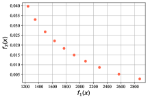
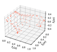
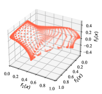
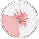
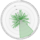
In this work, we investigate a new approach for many-objective optimization, which aims to find a small set of solutions (e.g., ) to handle a large number of objectives (e.g., ). In the optimal case, each objective should be well addressed by at least one solution in the small solution set as illustrated in Figure 1(d). This setting is important for different real-world applications with many objectives to optimize, such as finding complementary engineering designs to satisfy various criteria [19], producing a few different versions of advertisements to serve a large group of diverse audiences [44, 15], and building a small set of models to handle many different data [59, 62] or tasks [55, 18]. However, this demand has received little attention from the multi-objective optimization community. To properly handle this setting, this work makes the following contributions:
-
•
We propose a novel Tchebycheff set (TCH-Set) scalarization approach to find a few optimal solutions in a collaborative and complementary manner for many-objective optimization.
-
•
We further develop a smooth Tchebycheff set (STCH-Set) scalarization approach to tackle the non-smoothness of TCH-Set scalarization for efficient gradient-based optimization.
-
•
We provide theoretical analyses to show that both the proposed TCH-Set and STCH-Set scalarization approaches enjoy good theoretical properties for multi-objective optimization.
-
•
We conduct experiments on various multi-objective optimization problems with many objectives to demonstrate the efficiency of our proposed method. 111Our code to reproduce all experimental results will be released upon publication.
2 Preliminaries and Related Work
2.1 Multi-Objective Optimization

In this work, we consider the following multi-objective optimization problem:
| (1) |
where is a solution and are differentiable objective functions. For a non-trivial problem, there is no single solution that can optimize all objective functions at the same time. Therefore, we have the following definitions of dominance, (weakly) Pareto optimality, and Pareto set/front for multi-objective optimization [45]:
Definition 1 (Dominance and Strict Dominance).
Let be two solutions for problem (1), is said to dominate , denoted as , if and only if and . In addition, is said to strictly dominate (i.e., ), if and only if .
Definition 2 ((Weakly) Pareto Optimality).
A solution is Pareto optimal if there is no such that . A solution is weakly Pareto optimal if there is no such that .
Definition 3 (Pareto Set and Pareto Front).
The set of all Pareto optimal solutions is called the Pareto set. Its image in the objective space is called the Pareto front.
Under mild conditions, the Pareto set and front could be on an -dimensional manifold in the decision or objective space [26], which contains infinite Pareto solutions. Many optimization methods have been proposed to find a finite set of solutions to approximate the Pareto set and front [45, 16, 63]. If at least solutions are needed to handle each dimension of the Pareto front, the required number of solutions could be for a problem with optimization objectives. Two illustrative examples with a set of solutions to approximate the Pareto front for problems with and objectives are shown in Figure 1. However, the required number of solutions will increase exponentially with the objective number , leading to an extremely high computational overhead. It could also be very challenging for decision-makers to efficiently handle such a large set of solutions. Indeed, for a problem with many optimization objectives, a large portion of the solutions could become non-dominated and hence incomparable with each other [49, 29].
In the past few decades, different heuristic and evolutionary algorithms have been proposed to tackle the many-objective black-box optimization problems [61, 3, 12]. These algorithms typically aim to find a set of a few hundred solutions to handle problems with to a few dozen optimization objectives [30, 51]. However, they still struggle to tackle problems with significantly many objectives (e.g., ), and cannot efficiently solve large-scale differentiable optimization problems.
2.2 Gradient-based Multi-Objective Optimization
When all objective functions are differentiable with gradient , we have the following definition for Pareto stationarity:
Definition 4 (Pareto Stationary Solution).
A solution is Pareto stationary if there exists a set of weights such that the convex combination of gradients .
Multiple Gradient Descent Algorithm
One popular gradient-based approach is to find a valid gradient direction such that the values of all objective functions can be simultaneously improved [20, 52, 13]. The multiple gradient descent algorithm (MGDA) [13, 53] obtains a valid gradient by solving the following quadratic programming problem at each iteration:
| (2) |
and updates the current solution by a simple gradient descent . If , it means that there is no valid gradient direction that can improve all objectives at the same time, and therefore is a Pareto stationary solution [13, 21]. This idea has inspired many adaptive gradient methods for multi-task learning [46, 60, 35, 37, 39, 47, 54, 32, 36, 25]. Different stochastic multiple gradient methods have also been proposed in recent years [38, 64, 17, 8, 58].
The location of solutions found by the original MGDA is not controllable, and several extensions have been proposed to find a set of diverse solutions with different trade-offs [33, 43, 42, 40]. However, a large number of solutions is still required for a good approximation to the Pareto front. For solving problems with many objectives, MGDA and its extensions will suffer from a high computational overhead due to the high-dimensional quadratic programming problem (2) at each iteration. In addition, since a large portion of solutions is non-dominated with each other, it could be very hard to find a valid gradient direction to optimize all objectives at the same time.
Scalarization Method
Another popular class of methods for multi-objective optimization is the scalarization approach [45, 61]. The most straightforward method is linear scalarization [22]:
| (Linear Scalarization) | (3) |
where is a preference vector over objectives on the simplex . A set of diverse solutions can be obtained by solving the scalarization problem (3) with different preferences. Although it is simple and straightforward, linear scalarization cannot find any Pareto solution on the non-convex part of the Pareto front [11, 16].
Many other scalarization methods have been proposed in past decades. Among them, the Tchebycheff scalarization with good theoretical properties is a promising alternative [6, 56]:
| (Tchebycheff Scalarization) | (4) |
where is the preference and is the ideal point (e.g., with a small ). It is well-known that the Tchebycheff scalarization is able to find all weakly Pareto solutions for any Pareto front [10]. However, the operator makes it become nonsmooth and hence suffers from a slow convergence rate by subgradient descent [23] for differentiable multi-objective optimization. Recently, a smooth Tchebycheff scalarization approach [34] has been proposed to tackle the nonsmoothness issue:
| (Smooth Tchebycheff Scalarization) | (5) |
where is the smooth parameter with a small positive value (e.g., ). According to [34], this smooth scalarization approach enjoys a fast convergence rate for the gradient-based method, while also having good theoretical properties for multi-objective optimization.
These scalarization methods do not have to solve a quadratic programming problem at each iteration and thus have lower pre-iteration complexity than MGDA. However, they still need to solve a large number of scalarization problems with different preferences to obtain a dense set of solutions to approximate the whole Pareto set.
3 Tchebycheff Set Scalarization for Many Objective Optimization
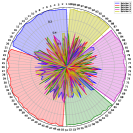
3.1 Small Solution Set for Many-Objective Optimization
Unlike previous methods, this work does not aim to find a huge set of solutions for approximating the whole Pareto set. Instead, we want to find a small set of solutions in a collaborative and complementary way such that each optimization objective can be well addressed by at least one solution. We have the following formulation of our targeted set optimization problem:
| (6) |
where is a set of solutions to tackle all objectives . With a large , we will have a degenerated problem:
| (7) |
where each objective function is independently solved by its corresponding solution via single objective optimization and the rest solutions are redundant. If , the set optimization problem (6) will be reduced to the standard multi-objective optimization problem (1).
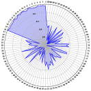
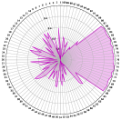
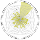
In this work, we are more interested in the case , which finds a small set of solutions (e.g., ) to tackle a large number of objectives (e.g., ) as illustrated in Figure 2. Very recently, a similar setting has been investigated in two concurrent works [14, 31]. Ding et al.[14] study the sum-of-minimum (SoM) optimization problem that can be found in many machine learning applications such as mixed linear regression [59, 62]. They generalize the classic k-means++ [2] and Lloyd’s algorithm [41] for clustering to tackle this problem, but do not take multi-objective optimization into consideration. Li et al. [31] propose a novel Many-objective multi-solution Transport (MosT) framework to tackle many-objective optimization. With a bi-level optimization formulation, they adaptively construct a few weighted multi-objective optimization problems that are assigned to different representative regions on the Pareto front. By solving these weighted problems with MGDA, a diverse set of solutions can be obtained to well cover all objectives. In this work, we propose a straightforward and efficient set scalarization approach to explicitly optimize all objectives by a small set of solutions. A detailed experimental comparison with these methods can be found in Section 4.
3.2 Tchebycheff Set Scalarization
The set optimization formulation (6) is still a multi-objective optimization problem. In non-trivial cases, there is no single small solution set with solutions that can optimize all objective functions at the same time. To tackle this optimization problem, we propose the following Tchebycheff set (TCH-Set) scalarization approach:
| (8) |
where and are the preference and ideal point for each objective function. In this way, all objective values among the whole solution set are scalarized into a single function . A simple uniform vector can be used if there is no specific preference among the objectives. By optimizing this TCH-Set scalarization function (8), we want to find an optimal small solution set such that each objective can be well addressed by at least one solution with a low worst objective value . When the solution set contains only one single solution (e.g., ), it will be reduced to the classic single-solution Tchebycheff scalarization (4).
In this work, we assume that no pair of the optimization objectives will share exactly the same optimal solution. Therefore, no solution in the optimal solution set will be redundant, which means
| (9) |
holds for any with a all positive preference . In addition, the optimal solution set also enjoys a good theoretical property for multi-objective optimization:
Theorem 1 (Pareto Optimality for Tchebycheff Set Scalarization).
Proof Sketch.
In other words, a small set of (weakly) Pareto solutions can be found by solving the TCH-Set scalarization optimization problem (8), which complementarily addresses all objectives to achieve a low worst performance . However, the non-smoothness of TCH-Set scalarization might hinder its practical usage for efficient optimization.
3.3 Smooth Tchebycheff Set Scalarization
The Tchebycheff set scalarization formulation (8) involves a and a operator, which leads to its non-smoothness even when all objective functions are smooth. In other words, the Tchebycheff set scalarization is not differentiable and will suffer from a slow convergence rate by subgradient descent. To address this issue, we leverage the smooth optimization approach [48, 4, 9] to propose a smooth Tchebycheff set scalarization for multi-objective optimization.
According to [4], for the maximization among all objectives , we have the smooth maximization function:
| (10) |
where is a smooth parameter. Similarly, for the minimization among different solutions for the -th objective , we have the smooth minimization function:
| (11) |
where is a smooth parameter.
By leveraging the above smooth maximization and minimization functions, we propose the smooth Tchebycheff set scalarization (STCH-Set) scalarization for multi-objective optimization:
| (12) |
If the same smooth parameter are used for all smooth terms, we have the following simplified formulation:
| (13) |
When , it will reduce to the single-solution smooth Tchebycheff scalarization (5). Similarly to the non-smooth TCH-Set counterpart, the STCH-Set scalarization also has good theoretical properties for multi-objective optimization:
Theorem 2 (Pareto Optimality for Smooth Tchebycheff Set Scalarization).
All solutions in the optimal solution set for the smooth Tchebycheff set scalarization problem (12) are weakly Pareto optimal of the original multi-objective optimization problem (1). In addition, the solutions are Pareto optimal if either
-
1.
the optimal solution set is unique, or
-
2.
all preference coefficients are positive ().
Proof Sketch.
Theorem 3 (Uniform Smooth Approximation).
The smooth Tchebycheff set (STCH-Set) scalarization is a uniform smooth approximation of the Tchebycheff set (TCH-Set) scalarization , and we have:
| (14) |
for any valid set .
Proof Sketch.
This theorem can be proved by deriving the upper and lower bounds of the TCH-Set scalarization with respect to the smooth and operators in the STCH-Set scalarization . A detailed proof is provided in Appendix A.3. ∎
According to these theorems, for any smooth parameters and , all solutions in the optimal set for STCH-Set scalarization (12) are also (weakly) Pareto optimal. In addition, with small smooth parameters , the value of will be close to its non-smooth counterpart for all valid solution sets , which is also the case for the optimal set . Therefore, it is reasonable to find an approximate optimal solution set for the original by optimizing its smooth counterpart with small smooth parameters and .
The STCH-Set scalarization function can be efficiently optimized by any gradient-based optimization method. A simple gradient descent algorithm for STCH-Set is shown in Algorithm 1. However, when the objective functions are highly non-convex, it could be very hard to find the global optimal set for . In this case, we have the Pareto stationarity guarantee for the gradient-based method:
Theorem 4 (Convergence to Pareto Stationary Solution).
If there exists a solution set such that for all , then all solutions in are Pareto stationary solutions of the original multi-objective optimization problem (1).
Proof Sketch.
When reduces to , all these theorems exactly match their counterpart theorems for single-solution Tchebycheff scalarization [10, 45] and smooth Tchebycheff scalarization [34].
| LS | TCH | STCH | MosT | SoM | TCH-Set | STCH-Set | ||
| number of objectives | ||||||||
| worst | 4.64e+00(+) | 4.44e+00(+) | 4.41e+00(+) | 2.12e+00(+) | 1.86e+00(+) | 1.02e+00(+) | 6.08e-01 | |
| K = 3 | average | 8.61e-01(+) | 8.03e-01(+) | 7.80e-01(+) | 3.45e-01(+) | 2.02e-01(-) | 3.46e-01(+) | 2.12e-01 |
| worst | 4.23e+00(+) | 3.83e+00(+) | 3.68e+00(+) | 1.48e+00(+) | 1.12e+00(+) | 6.74e-01(+) | 3.13e-01 | |
| K = 4 | average | 7.45e-01(+) | 6.54e-01(+) | 6.41e-01(+) | 1.85e-01(+) | 1.12e-01(+) | 2.27e-01(+) | 9.44e-02 |
| worst | 4.17e+00(+) | 3.56e+00(+) | 3.51e+00(+) | 1.02e+00(+) | 9.20e-01(+) | 4.94e-01(+) | 1.91e-01 | |
| K = 5 | average | 7.08e-01(+) | 5.75e-01(+) | 5.05e-01(+) | 9.81e-02(+) | 7.95e-02(+) | 1.60e-01(+) | 5.12e-02 |
| worst | 3.81e+00(+) | 3.41e+00(+) | 3.20e+00(+) | 9.56e-01(+) | 7.03e-01(+) | 3.72e-01(+) | 1.36e-01 | |
| K = 6 | average | 6.72e-01(+) | 5.31e-01(+) | 5.15e-01(+) | 8.34e-02(+) | 5.34e-02(+) | 1.19e-01(+) | 3.15e-02 |
| worst | 3.69e+00(+) | 2.94e+00(+) | 2.61e+00(+) | 8.32e-01(+) | 5.20e-01(+) | 2.84e-01(+) | 1.02e-01 | |
| K = 8 | average | 6.16e-01(+) | 4.57e-01(+) | 4.22e-01(+) | 6.91e-02(+) | 3.40e-02(+) | 8.53e-02(+) | 1.78e-02 |
| worst | 3.68e+00(+) | 2.69e+00(+) | 2.40e+00(+) | 6.27e-01(+) | 4.07e-01(+) | 1.95e-01(+) | 7.99e-02 | |
| K = 10 | average | 5.69e-01(+) | 4.07e-01(+) | 3.20e-01(+) | 4.59e-02(+) | 2.43e-02(+) | 5.92e-02(+) | 1.34e-02 |
| number of objectives | ||||||||
| worst | 4.71e+00(+) | 7.84e+00(+) | 7.33e+00(+) | - | 3.36e+00(+) | 2.39e+00(+) | 1.87e+00 | |
| K = 3 | average | 1.15e+00(+) | 9.92e-01(+) | 9.70e-01(+) | - | 3.54e-01(-) | 4.55e-01(+) | 3.92e-01 |
| worst | 4.48e+00(+) | 6.77e+00(+) | 6.57e+00(+) | - | 2.34e+00(+) | 1.68e+00(+) | 9.93e-01 | |
| K = 5 | average | 1.09e+00(+) | 8.02e-01(+) | 7.65e-01(+) | - | 1.95e-01(+) | 2.59e-01(+) | 1.87e-01 |
| worst | 4.25e+00(+) | 5.65e+00(+) | 5.58e+00(+) | - | 1.74e+00(+) | 1.25e+00(+) | 4.90e-01 | |
| K = 8 | average | 1.03e+00(+) | 6.69e-01(+) | 6.49e-01(+) | - | 1.02e-01(+) | 1.66e-01(+) | 8.31e-02 |
| worst | 4.16e+00(+) | 5.61e+00(+) | 5.44e+00(+) | - | 1.78e+00(+) | 1.16e+00(+) | 4.05e-01 | |
| K = 10 | average | 1.00e+00(+) | 6.07e-01(+) | 5.99e-01(+) | - | 8.14e-02(+) | 1.41e-01(+) | 5.94e-02 |
| worst | 4.06e+00(+) | 4.78e+00(+) | 4.91e+00(+) | - | 1.54e+00(+) | 9.06e-01(+) | 2.85e-01 | |
| K = 15 | average | 9.78e-01(+) | 5.15e-01(+) | 4.99e-01(+) | - | 5.98e-02(+) | 1.01e-01(+) | 3.31e-02 |
| worst | 3.97e+00(+) | 4.64e+00(+) | 4.57e+00(+) | - | 1.52e+00(+) | 8.04e-01(+) | 2.28e-01 | |
| K = 20 | average | 9.56e-01(+) | 4.63e-01(+) | 4.68e-01(+) | - | 5.30e-02(+) | 8.40e-02(+) | 2.27e-02 |
| Wilcoxon Rank-Sum Test Summary | ||||||||
| worst | 12/0/0 | 12/0/0 | 12/0/0 | 6/0/0 | 12/0/0 | 12/0/0 | - | |
| +/=/- | average | 12/0/0 | 12/0/0 | 12/0/0 | 6/0/0 | 10/0/2 | 12/0/0 | - |
| LS | TCH | STCH | SoM | TCH-Set | STCH-Set | ||
|---|---|---|---|---|---|---|---|
| K = 5 | worst | 3.84e+01(+) | 2.45e+01(+) | 2.43e+01(+) | 2.50e+00(+) | 4.19e+00(+) | 2.10e+00 |
| average | 2.70e+00(+) | 1.46e+00(+) | 1.44e+00(+) | 1.88e-01(-) | 6.53e-01(+) | 4.72e-01 | |
| worst | 2.21e+01(+) | 2.49e+01(+) | 3.92e+01(+) | 3.46e+00(+) | 2.04e+00(+) | 5.00e-01 | |
| K = 10 | average | 1.09e+00(+) | 1.19e+00(+) | 3.01e+00(+) | 2.33e-01(+) | 3.83e-01(+) | 2.00e-01 |
| worst | 4.20e+01(+) | 2.11e+01(+) | 2.21e+01(+) | 2.57e+00(+) | 1.64e+00(+) | 2.70e-01 | |
| K = 15 | average | 3.07e+00(+) | 1.02e+00(+) | 1.02e+00(+) | 1.97e-01(+) | 3.22e-01(+) | 1.66e-01 |
| worst | 4.20e+01(+) | 2.14e+01(+) | 2.04e+01(+) | 1.44e+00(+) | 1.79e+00(+) | 2.27e-01 | |
| K = 20 | average | 3.09e+00(+) | 8.35e-01(+) | 8.87e-01(+) | 1.84e-01(+) | 3.29e-01(+) | 1.66e-01 |
4 Experiments
Baseline Methods
In this section, we compare our proposed TCH-Set and STCH-Set scalarization with (1) linear scalarization (LS) with randomly sampled preferences, (2) Tchebycheff scalarization (TCH) with randomly sampled preferences, (3) smooth Tchebycheff scalarization (STCH) with randomly sampled preferences [34], (4) the many-objective multi-solution transport (MosT) method [31], and (5) the efficient sum-of-minimum (SoM) optimization method [14].
Experimental Setting
This work aims to find a small set with solutions to address all objectives in each problem. For each objective , we care about the best objective value achieved by the solutions in . Both the worst obtained value among all objectives and the average objective value are reported for comparison. Detailed experimental settings for each problem can be found in Appendix B.
4.1 Experimental Results and Analysis
Convex Many-Objective Optimization
We first test our proposed methods for solving convex multi-objective optimization with or objective functions with different numbers of solutions (from to ). We independently run each comparison times. In each run, we randomly generate independent convex quadratic functions as the optimization objectives for all methods. The mean worst and average objective values for each method over runs are reported in Table 1. We also conduct the Wilcoxon rank-sum test between STCH-Set and other methods for all comparisons at the significant level. The symbol means the result obtained by STCH-Set is significantly better, equal to, or worse than the results of the compared method.
According to the results, the traditional methods (e.g., LS/TCH/STCH) fail to properly tackle the few solutions for many objectives setting considered in this work. MosT achieves much better performance than the traditional methods by actively finding a set of diverse solutions to cover all objectives, but it cannot tackle the problems with objectives in a reasonable time. In addition, MosT is outperformed by SoM and our proposed STCH-Set, which directly optimizes the performance for each objective. Our proposed STCH-Set performs the best in achieving the low worst objective values for all comparisons. In addition, although not explicitly designed, STCH-Set also achieves a very promising mean average performance for most comparisons since all objectives are well addressed. The importance of smoothness for set optimization is fully confirmed by the observation that STCH-Set significantly outperforms TCH-Set on all comparisons.
| LS | TCH | STCH | SoM | TCH-Set | STCH-Set | ||
|---|---|---|---|---|---|---|---|
| K = 5 | worst | 2.34e+02 (+) | 1.68e+02(+) | 1.57e+02(+) | 1.68e+01(+) | 1.94e+01(+) | 7.43e+00 |
| average | 9.19e+00(+) | 8.50e+00(+) | 7.90e+00(+) | 8.54e-01(-) | 3.48e+00(+) | 1.89e+00 | |
| worst | 3.23e+02(+) | 1.72e+02(+) | 1.57e+02(+) | 4.42e+00(+) | 6.07e+00(+) | 6.28e-01 | |
| K = 10 | average | 8.70e+00 (+) | 6.65e+00(+) | 5.85e+00(+) | 1.22e-01(+) | 1.03e+00(+) | 5.99e-02 |
| worst | 3.65e+02(+) | 2.10e+02(+) | 1.62e+02(+) | 1.10e+00(+) | 1.57e+00(+) | 2.05e-01 | |
| K = 15 | average | 8.33e+00(+) | 5.66e+00(+) | 4.89e+00(+) | 1.47e-01(+) | 3.27e-01(+) | 1.27e-02 |
| worst | 3.36e+02(+) | 2.04e+02(+) | 1.81e+02(+) | 5.59e+00(+) | 4.37e+00(+) | 6.22e-01 | |
| K = 20 | average | 8.81e+00(+) | 6.92e+00(+) | 6.23e+00(+) | 1.24e-01(+) | 9.09e-01(+) | 6.27e-02 |
Noisy Mixed Linear Regression
We then test different methods’ performance on the noisy mixed linear regression problem as in [14]. For each comparison, data points are randomly generated from ground truth linear models with noise. Then, with different optimization methods, we train linear regression models to tackle all data points where the objectives are the squared error for each point. Each comparison are run times, and the detailed experiment setting is in Appendix B.
We conduct comparison with different numbers of and noise levels . The results with are shown in Table 2, and the full results can be found in Appendix C.1. According to the results, our proposed STCH-Set can always achieve the lowest worst objective value, and achieves the best average objective value in most comparisons.
Noisy Mixed Nonlinear Regression
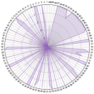
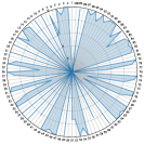
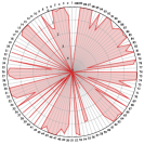
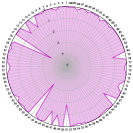
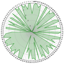
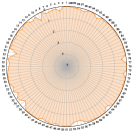
Following [14], we also compare different methods on the noisy mixed nonlinear regression. The problem setting (details in Appendix B) is similar to the mixed linear regression, but we now build simple nonlinear neural networks as the models. According to the results in Table 3 and Appendix C.2, STCH-Set can still obtain the best overall performance for most comparisons. We visualize different methods’ performance on sampled data in Figure 3.
5 Conclusion, Limitation and Future Work
Conclusion
In this work, we have proposed a novel Tchebycheff set (TCH-Set) scalarization and a smooth Tchebycheff set (STCH-Set) scalarization to find a small set of solutions for many-objective optimization. When properly optimized, each objective in the original problem should be well addressed by at least one solution in the found solution set. Both theoretical analysis and experimental studies have been conducted to demonstrate the promising properties and efficiency of TCH-Set/STCH-Set. Our proposed methods could provide a promising alternative to the current methods for tackling many-objective optimization.
Limitation and Future Work
This work proposes general optimization methods for multi-objective optimization which are not tied to particular applications. We do not see any specific potential societal impact of the proposed methods. This work only focuses on the deterministic optimization setting that all objectives are always available. One potential future research direction is to investigate how to deal with only partially observable objective values in practice.
References
- Adriana et al. [2018] S. Adriana, W. Harrison, C. Eitan, S. Justin, and M. Wojciech. Interactive exploration of design trade-offs. Acm Transactions on Graphics, 37(4):1–14, 2018.
- Arthur [2007] D. Arthur. K-means++: The advantages of careful seeding. In Proc. Eighteenth Annual ACM-SIAM Symposium on Discrete Algorithms, pages 1027–1035, 2007.
- Bader and Zitzler [2011] J. Bader and E. Zitzler. Hype: An algorithm for fast hypervolume-based many-objective optimization. Evolutionary computation, 19(1):45–76, 2011.
- Beck and Teboulle [2012] A. Beck and M. Teboulle. Smoothing and first order methods: A unified framework. SIAM Journal on Optimization, 22(2):557–580, 2012.
- Bertsekas et al. [2003] D. Bertsekas, A. Nedic, and A. Ozdaglar. Convex analysis and optimization, volume 1. Athena Scientific, 2003.
- Bowman [1976] V. J. Bowman. On the relationship of the tchebycheff norm and the efficient frontier of multiple-criteria objectives. In Multiple criteria decision making, pages 76–86. Springer, 1976.
- Boyd and Vandenberghe [2004] S. Boyd and L. Vandenberghe. Convex optimization. Cambridge university press, 2004.
- Chen et al. [2023] L. Chen, H. Fernando, Y. Ying, and T. Chen. Three-way trade-off in multi-objective learning: Optimization, generalization and conflict-avoidance. In Advances in Neural Information Processing Systems (NeurIPS), 2023.
- Chen [2012] X. Chen. Smoothing methods for nonsmooth, nonconvex minimization. Mathematical programming, 134:71–99, 2012.
- Choo and Atkins [1983] E. U. Choo and D. Atkins. Proper efficiency in nonconvex multicriteria programming. Mathematics of Operations Research, 8(3):467–470, 1983.
- Das and Dennis [1997] I. Das and J. Dennis. A closer look at drawbacks of minimizing weighted sums of objectives for pareto set generation in multicriteria optimization problems. Structural Optimization, 14(1):63–69, 1997.
- Deb and Jain [2013] K. Deb and H. Jain. An evolutionary many-objective optimization algorithm using reference-point-based nondominated sorting approach, part i: solving problems with box constraints. IEEE transactions on evolutionary computation, 18(4):577–601, 2013.
- Désidéri [2012] J.-A. Désidéri. Mutiple-gradient descent algorithm for multiobjective optimization. In European Congress on Computational Methods in Applied Sciences and Engineering (ECCOMAS 2012), 2012.
- Ding et al. [2024] L. Ding, Z. Chen, X. Wang, and W. Yin. Efficient algorithms for sum-of-minimum optimization. arXiv preprint arXiv:2402.07070, 2024.
- Eckles et al. [2018] D. Eckles, B. R. Gordon, and G. A. Johnson. Field studies of psychologically targeted ads face threats to internal validity. Proceedings of the National Academy of Sciences, 115(23):E5254–E5255, 2018.
- Ehrgott [2005] M. Ehrgott. Multicriteria optimization, volume 491. Springer Science & Business Media, 2005.
- Fernando et al. [2023] H. D. Fernando, H. Shen, M. Liu, S. Chaudhury, K. Murugesan, and T. Chen. Mitigating gradient bias in multi-objective learning: A provably convergent approach. In International Conference on Learning Representations (ICLR), 2023.
- Fifty et al. [2021] C. Fifty, E. Amid, Z. Zhao, T. Yu, R. Anil, and C. Finn. Efficiently identifying task groupings for multi-task learning. Advances in Neural Information Processing Systems (NeurIPS), 2021.
- Fleming et al. [2005] P. J. Fleming, R. C. Purshouse, and R. J. Lygoe. Many-objective optimization: An engineering design perspective. In International conference on evolutionary multi-criterion optimization, pages 14–32. Springer, 2005.
- Fliege and Svaiter [2000] J. Fliege and B. F. Svaiter. Steepest descent methods for multicriteria optimization. Mathematical Methods of Operations Research, 51(3):479–494, 2000.
- Fliege et al. [2019] J. Fliege, A. I. F. Vaz, and L. N. Vicente. Complexity of gradient descent for multiobjective optimization. Optimization Methods and Software, 34(5):949–959, 2019.
- Geoffrion [1967] A. M. Geoffrion. Solving bicriterion mathematical programs. Operations Research, 15(1):39–54, 1967.
- Goffin [1977] J.-L. Goffin. On convergence rates of subgradient optimization methods. Mathematical programming, 13:329–347, 1977.
- Hayes et al. [2022] C. F. Hayes, R. Rădulescu, E. Bargiacchi, J. Källström, M. Macfarlane, M. Reymond, T. Verstraeten, L. M. Zintgraf, R. Dazeley, F. Heintz, et al. A practical guide to multi-objective reinforcement learning and planning. Autonomous Agents and Multi-Agent Systems, 36(1):26, 2022.
- He et al. [2024] Y. He, S. Zhou, G. Zhang, H. Yun, Y. Xu, B. Zeng, T. Chilimbi, and H. Zhao. Robust multi-task learning with excess risks. arXiv preprint arXiv:2402.02009, 2024.
- Hillermeier [2001] C. Hillermeier. Generalized homotopy approach to multiobjective optimization. Journal of Optimization Theory and Applications, 110(3):557–583, 2001.
- Ishibuchi et al. [2008] H. Ishibuchi, N. Tsukamoto, and Y. Nojima. Evolutionary many-objective optimization: A short review. In IEEE congress on evolutionary computation (IEEE world congress on computational intelligence), pages 2419–2426. IEEE, 2008.
- Jain et al. [2023] M. Jain, S. C. Raparthy, A. Hernández-García, J. Rector-Brooks, Y. Bengio, S. Miret, and E. Bengio. Multi-objective GFlowNets. In International Conference on Machine Learning (ICML), pages 14631–14653. PMLR, 2023.
- Knowles and Corne [2007] J. Knowles and D. Corne. Quantifying the effects of objective space dimension in evolutionary multiobjective optimization. In Evolutionary Multi-Criterion Optimization: 4th International Conference, EMO 2007, Matsushima, Japan, March 5-8, 2007. Proceedings 4, pages 757–771. Springer, 2007.
- Li et al. [2015] B. Li, J. Li, K. Tang, and X. Yao. Many-objective evolutionary algorithms: A survey. ACM Computing Surveys (CSUR), 48(1):1–35, 2015.
- Li et al. [2024] Z. Li, T. Li, V. Smith, J. Bilmes, and T. Zhou. Many-objective multi-solution transport. arXiv preprint arXiv:2403.04099, 2024.
- Lin et al. [2023] B. Lin, W. Jiang, F. Ye, Y. Zhang, P. Chen, Y.-C. Chen, S. Liu, and J. T. Kwok. Dual-balancing for multi-task learning, 2023.
- Lin et al. [2019] X. Lin, H.-L. Zhen, Z. Li, Q. Zhang, and S. Kwong. Pareto multi-task learning. In Advances in Neural Information Processing Systems, pages 12060–12070, 2019.
- Lin et al. [2024] X. Lin, X. Zhang, Z. Yang, F. Liu, Z. Wang, and Q. Zhang. Smooth tchebycheff scalarization for multi-objective optimization. arXiv preprint arXiv:2402.19078, 2024.
- Liu et al. [2021a] B. Liu, X. Liu, X. Jin, P. Stone, and Q. Liu. Conflict-averse gradient descent for multi-task learning. Advances in Neural Information Processing Systems (NeurIPS), 34:18878–18890, 2021a.
- Liu et al. [2024] B. Liu, Y. Feng, P. Stone, and Q. Liu. Famo: Fast adaptive multitask optimization. Advances in Neural Information Processing Systems (NeurIPS), 36, 2024.
- Liu et al. [2021b] L. Liu, Y. Li, Z. Kuang, J. Xue, Y. Chen, W. Yang, Q. Liao, and W. Zhang. Towards impartial multi-task learning. In International Conference on Learning Representations (ICLR), 2021b.
- Liu and Vicente [2021] S. Liu and L. N. Vicente. The stochastic multi-gradient algorithm for multi-objective optimization and its application to supervised machine learning. Annals of Operations Research, pages 1–30, 2021.
- Liu et al. [2022] S. Liu, S. James, A. Davison, and E. Johns. Auto-lambda: Disentangling dynamic task relationships. Transactions on Machine Learning Research, 2022.
- Liu et al. [2021c] X. Liu, X. Tong, and Q. Liu. Profiling pareto front with multi-objective stein variational gradient descent. Advances in Neural Information Processing Systems (NeurIPS), 34:14721–14733, 2021c.
- Lloyd [1982] S. Lloyd. Least squares quantization in pcm. IEEE transactions on information theory, 28(2):129–137, 1982.
- Ma et al. [2020] P. Ma, T. Du, and W. Matusik. Efficient continuous pareto exploration in multi-task learning. International Conference on Machine Learning (ICML), 2020.
- Mahapatra and Rajan [2020] D. Mahapatra and V. Rajan. Multi-task learning with user preferences: Gradient descent with controlled ascent in pareto optimization. Thirty-seventh International Conference on Machine Learning, 2020.
- Matz et al. [2017] S. C. Matz, M. Kosinski, G. Nave, and D. J. Stillwell. Psychological targeting as an effective approach to digital mass persuasion. Proceedings of the national academy of sciences, 114(48):12714–12719, 2017.
- Miettinen [1999] K. Miettinen. Nonlinear multiobjective optimization, volume 12. Springer Science & Business Media, 1999.
- Momma et al. [2022] M. Momma, C. Dong, and J. Liu. A multi-objective/multi-task learning framework induced by pareto stationarity. In International Conference on Machine Learning (ICML), pages 15895–15907. PMLR, 2022.
- Navon et al. [2022] A. Navon, A. Shamsian, I. Achituve, H. Maron, K. Kawaguchi, G. Chechik, and E. Fetaya. Multi-task learning as a bargaining game. In International Conference on Machine Learning (ICML), pages 16428–16446. PMLR, 2022.
- Nesterov [2005] Y. Nesterov. Smooth minimization of non-smooth functions. Mathematical Programming, 103:127–152, 2005.
- Purshouse and Fleming [2007] R. C. Purshouse and P. J. Fleming. On the evolutionary optimization of many conflicting objectives. IEEE transactions on evolutionary computation, 11(6):770–784, 2007.
- Roijers et al. [2014] D. M. Roijers, P. Vamplew, S. Whiteson, and R. Dazeley. A survey of multi-objective sequential decision-making. Journal of Artificial Intelligence Research, 48(1):67–113, 2014.
- Sato and Ishibuchi [2023] H. Sato and H. Ishibuchi. Evolutionary many-objective optimization: Difficulties, approaches, and discussions. IEEJ Transactions on Electrical and Electronic Engineering, 18(7):1048–1058, 2023.
- Schäffler et al. [2002] S. Schäffler, R. Schultz, and K. Weinzierl. Stochastic method for the solution of unconstrained vector optimization problems. Journal of Optimization Theory and Applications, 114:209–222, 2002.
- Sener and Koltun [2018] O. Sener and V. Koltun. Multi-task learning as multi-objective optimization. In Advances in Neural Information Processing Systems, pages 525–536, 2018.
- Senushkin et al. [2023] D. Senushkin, N. Patakin, A. Kuznetsov, and A. Konushin. Independent component alignment for multi-task learning. In IEEE/CVF Conference on Computer Vision and Pattern Recognition (CVPR), pages 20083–20093, 2023.
- Standley et al. [2020] T. Standley, A. Zamir, D. Chen, L. Guibas, J. Malik, and S. Savarese. Which tasks should be learned together in multi-task learning? In International Conference on Machine Learning (ICML), pages 9120–9132. PMLR, 2020.
- Steuer and Choo [1983] R. E. Steuer and E.-U. Choo. An interactive weighted tchebycheff procedure for multiple objective programming. Mathematical programming, 26(3):326–344, 1983.
- Wang et al. [2020] H. Wang, K. Wang, J. Yang, L. Shen, N. Sun, H.-S. Lee, and S. Han. Gcn-rl circuit designer: Transferable transistor sizing with graph neural networks and reinforcement learning. In 2020 57th ACM/IEEE Design Automation Conference (DAC), pages 1–6. IEEE, 2020.
- Xiao et al. [2023] P. Xiao, H. Ban, and K. Ji. Direction-oriented multi-objective learning: Simple and provable stochastic algorithms. In Advances in Neural Information Processing Systems (NeurIPS), 2023.
- Yi et al. [2014] X. Yi, C. Caramanis, and S. Sanghavi. Alternating minimization for mixed linear regression. In International Conference on Machine Learning, pages 613–621. PMLR, 2014.
- Yu et al. [2020] T. Yu, S. Kumar, A. Gupta, S. Levine, K. Hausman, and C. Finn. Gradient surgery for multi-task learning. Advances in Neural Information Processing Systems (NeurIPS), 33:5824–5836, 2020.
- Zhang and Li [2007] Q. Zhang and H. Li. MOEA/D: A multiobjective evolutionary algorithm based on decomposition. IEEE Transactions on evolutionary computation, 11(6):712–731, 2007.
- Zhong et al. [2016] K. Zhong, P. Jain, and I. S. Dhillon. Mixed linear regression with multiple components. Advances in neural information processing systems, 29, 2016.
- Zhou et al. [2011] A. Zhou, B.-Y. Qu, H. Li, S.-Z. Zhao, P. N. Suganthan, and Q. Zhang. Multiobjective evolutionary algorithms: A survey of the state of the art. Swarm and Evolutionary Computation, 1(1):32–49, 2011.
- Zhou et al. [2022] S. Zhou, W. Zhang, J. Jiang, W. Zhong, J. Gu, and W. Zhu. On the convergence of stochastic multi-objective gradient manipulation and beyond. In Advances in Neural Information Processing Systems (NeurIPS), 2022.
- Zhu et al. [2023] Y. Zhu, J. Wu, C. Hu, J. Yan, T. Hou, J. Wu, et al. Sample-efficient multi-objective molecular optimization with gflownets. Advances in Neural Information Processing Systems, 36, 2023.
In this appendix, we mainly provide:
Appendix A Detailed Proof
A.1 Proof of Theorem 1
Theorem 1 (Pareto Optimality for Tchebycheff Set Scalarization). All solutions in the optimal solution set for the Tchebycheff set scalarization optimization problem (8) are weakly Pareto optimal of the original multi-objective optimization problem (1). In addition, if the optimal set is unique, all solutions in are Pareto optimal.
Proof.
Weakly Pareto Optimality
We first prove all the solutions in are weakly Pareto optimal. Let be an optimal solution set for the Tchebycheff set scalarization problem (8), we have:
| (15) |
where .
Without loss of generality, we further suppose the -th solution in is not weakly Pareto optimal for the original multi-objective optimization problem (1). According to Definition 2 for weakly Pareto optimality, there exists a valid solution such that . In other words, we have:
| (16) |
If we replace the solution in by (e.g., ), we have the new solution set . Based on the above inequalities, it is easy to check:
| (17) |
There is a contradiction between (17) and the optimality of for the Tchebycheff set scalarization (15). Therefore, every should be a weakly Pareto optimal solution for the original multi-objective optimization problem (1).
Pareto Optimality for Unique Optimal Solution Set
Similar to the above proof, without loss of generality, we suppose the -th solution in is not Pareto optimal, which means there exists a valid solution such that . In other words, we have:
| (18) |
Also let , we have:
| (19) |
On the other hand, according to the uniqueness of , we have:
| (20) |
The above two inequalities (19) and (20) are contradicted with each other. Therefore, every solution in the unique optimal solution set should be Pareto optimal.
∎
A.2 Proof of Theorem 2
Theorem 2 (Pareto Optimality for Smooth Tchebycheff Set Scalarization). All solutions in the optimal solution set for the smooth Tchebycheff set scalarization problem (12) are weakly Pareto optimal of the original multi-objective optimization problem (1). In addition, the solutions are Pareto optimal if either
-
1.
the optimal solution set is unique, or
-
2.
all preference coefficients are positive ().
Proof.
Weakly Pareto Optimality
We first prove all the solutions in are weakly Pareto optimal. Let be an optimal solution set for the smooth Tchebycheff set scalarization problem (12), we have:
| (21) |
where .
Without loss of generality, we further suppose the -th solution in is not weakly Pareto optimal for the original multi-objective optimization problem (1). According to Definition 2 for weakly Pareto optimality, there exists a valid solution such that . In other words, we have:
| (22) |
If we replace the solution in by (e.g., ), we have the new solution set . Based on the above inequalities, and further let and , it is easy to check:
| (23) |
There is a contradiction between (23) and the optimality of for the smooth Tchebycheff set scalarization (21). Therefore, every should be a weakly Pareto optimal solution for the original multi-objective optimization problem (1).
Then we prove the two sufficient conditions for all solutions in be Pareto optimal.
1. Unique Optimal Solution Set
Without loss of generality, we suppose the -th solution in is not Pareto optimal, which means there exists a valid solution such that . In other words, we have:
| (24) |
Also let where and , we have:
| (25) |
On the other hand, according to the uniqueness of , we have:
| (26) |
The above two inequalities (25) and (26) are contradicted with each other. Therefore, every solution in the unique optimal solution set should be Pareto optimal.
2. All Positive Preferences Similar to the above proof, suppose the solution is not Pareto optimal, and there exists a valid solution such that . Since all preferences are positive, according to the set of inequalities in (24), it is easy to check:
| (27) |
which contradicts the STCH-Set optimality of in (21). Therefore, all solutions in should be Pareto optimal.
It should be noted that all positive preferences are not a sufficient conditions for the solution to be Pareto optimal for the original (nonsmooth) Tchebycheff set (TCH-Set) scalarization. With all positive preferences, each component (e.g., all objective-solution pairs) in STCH-Set scalarization will contribute to the scalarization value, which is not the case for the (non-smooth) TCH-Set scalarization.
∎
A.3 Proof of Theorem 3
Theorem 3 (Uniform Smooth Approximation). The smooth Tchebycheff set (STCH-Set) scalarization is a uniform smooth approximation of the Tchebycheff set (TCH-Set) scalarization , and we have:
| (28) |
for any valid set .
Proof.
This theorem can be proved by deriving the upper and lower bounds of with respect to the smooth and operators in . We first provide the upper and lower bounds for the classic smooth approximation for and , and then derive the bounds for .
Classic Bounds for and
The log-sum-exp function is a widely-used smooth approximation for the maximization function . Its lower and upper bounds are also well-known in convex optimization [5, 7]:
| (29) |
By rearranging the above inequalities, we have:
| (30) |
With a smooth parameter , it is also easy to show [5, 7]:
| (31) |
Similarly, we have the lower and upper bounds for the minimization function:
| (32) |
Lower and Upper Bounds for
By leveraging the above classic bounds, it is straightforward to derive the lower and upper bounds for the operator over optimization objectives for :
| (33) | |||
| (34) |
where the bounds are tight if .
In a similar manner, we can obtain the bounds for the operator over solutions for each objective function :
| (35) |
where the bounds are tight if .
Combing the results above, we have the upper bound and lower bounds for the Tchebycheff setscalarization :
| (36) | |||
| (37) |
which means is properly bounded from above and below, and the bounds are tight if and for all . It is straightforward to see:
| (38) |
for all valid solution sets that include the optimal set . Therefore, according to Nesterov (2005) [48], is a uniform smooth approximation of .
∎
A.4 Proof of Theorem 4
Theorem 4 (Convergence to Pareto Stationary Solution). If there exists a solution set such that for all , then all solutions in are Pareto stationary solutions of the original multi-objective optimization problem (1).
Proof.
We can prove this theorem by analyzing the form of gradient for STCH-Set scalarization for each solution with the condition for Pareto stationarity in Definition 4.
We first let
| (39) | |||
| (40) | |||
| (41) |
For the STCH scalarization, we have:
| (42) | ||||
| (43) | ||||
| (44) | ||||
| (45) |
Therefore, according to the chain rule, the gradient of with respect to a solution in the set can be written as:
| (46) |
It is straightforward to show
| (47) |
Therefore, we have
| (48) |
Let , it is easy to check . If set and , we have:
| (49) | ||||
| (50) | ||||
| (51) |
where . For a solution , if , we have:
| (52) |
According to Definition 4, the solution is Pareto stationary for the multi-objective optimization problem (1).
Therefore, when for all , all solutions in are Pareto stationary for the original multi-objective optimization problem (1).
∎
Appendix B Problem and Experimental Settings
B.1 Convex Multi-Objective Optimization
In this experiment, we compare different methods on solving convex optimization problems with solutions. We consider two numbers of objectives and six different numbers of solutions or for the -objective and -objective problems separately. Therefore, there are total comparisons.
For each comparison, we randomly generate independent quadratic functions as the optimization objectives, of which the minimum values are all . Therefore, the optimal worst and average objective values are both for all comparisons. Since the objectives are randomly generated and with different optimal solution, the optimal worst and average objective value cannot be achieved by any algorithms unless . In all comparison, we let all solution be -dimensional vector . We repeat each comparison times and report the mean worst and average objective value over runs for each method.
B.2 Noisy Mixed Linear Regression
We follow the noisy mixed linear regression setting from [14]. The -th optimization objective is defined as:
| (53) |
where are data points and is a fixed penalty parameter. The dataset is randomly generated in the following steps:
-
•
Randomly sample i.i.d. ground truth ;
-
•
Randomly sample i.i.d. data , class index , and noise ;
-
•
Compute .
Our goal is to build linear model with parameter to tackle all data points. In this experiment, we set and for all comparisons. We consider three noise levels and four different numbers of solutions for each noise level, so there are total comparisons. All comparisons are run times, and we compare the mean worst and average objective values for each method.
B.3 Noisy Mixed Nonlinear Regression
The experimental setting for noisy mixed nonlinear regression is also from [14] and similar to the linear regression counterpart. For nonlinear regression, the -th optimization objective is defined as:
| (54) |
where are data points and is a fixed penalty parameter as in the previous linear regression case. However, now the model is a neural network with trainale model parameters with the form:
| (55) |
where and . The and are the input dimension and hidden dimension, respectively. The data set can be generated similar to linear regression but with ground truth neural network models. We set and in all comparisons.
Appendix C More Experimental Results
C.1 Noisy Mixed Linear Regression
| LS | TCH | STCH | SoM | TCH-Set | STCH-Set | ||
| K = 5 | worst | 3.84e+01(+) | 2.45e+01(+) | 2.43e+01(+) | 2.50e+00(+) | 4.19e+00(+) | 2.10e+00 |
| average | 2.70e+00(+) | 1.46e+00(+) | 1.44e+00(+) | 1.88e-01(-) | 6.53e-01(+) | 4.72e-01 | |
| worst | 2.21e+01(+) | 2.49e+01(+) | 3.92e+01(+) | 3.46e+00(+) | 2.04e+00(+) | 5.00e-01 | |
| K = 10 | average | 1.09e+00(+) | 1.19e+00(+) | 3.01e+00(+) | 2.33e-01(+) | 3.83e-01(+) | 2.00e-01 |
| worst | 4.20e+01(+) | 2.11e+01(+) | 2.21e+01(+) | 2.57e+00(+) | 1.64e+00(+) | 2.70e-01 | |
| K = 15 | average | 3.07e+00(+) | 1.02e+00(+) | 1.02e+00(+) | 1.97e-01(+) | 3.22e-01(+) | 1.66e-01 |
| worst | 4.20e+01(+) | 2.14e+01(+) | 2.04e+01(+) | 1.44e+00(+) | 1.79e+00(+) | 2.27e-01 | |
| K = 20 | average | 3.09e+00(+) | 8.35e-01(+) | 8.87e-01(+) | 1.84e-01(+) | 3.29e-01(+) | 1.66e-01 |
| worst | 3.93e+01(+) | 2.53e+01(+) | 2.50e+01(+) | 5.33e+00(+) | 4.37e+00(+) | 2.45e+00 | |
| K = 5 | average | 2.74e+00(+) | 1.51e+00(+) | 1.52e+00(+) | 3.08e-01(-) | 7.05e-01(+) | 5.54e-01 |
| worst | 4.20e+01(+) | 2.39e+01(+) | 2.56e+01(+) | 3.68e+00(+) | 2.38e+00(+) | 6.03e-01 | |
| K = 10 | average | 3.25e+00(+) | 1.28e+00(+) | 1.20e+00(+) | 2.46e-01(+) | 4.18e-01(+) | 2.24e-01 |
| worst | 4.36e+01(+) | 2.37e+01(+) | 2.35e+01(+) | 3.00e+00(+) | 1.72e+00(+) | 3.07e-01 | |
| K = 15 | average | 3.30e+00(+) | 1.02e+00(+) | 1.09e+00(+) | 2.06e-01(+) | 3.46e-01(+) | 1.78e-01 |
| worst | 4.36e+01(+) | 2.18e+01(+) | 2.23e+01(+) | 1.93e+00(+) | 1.27e+00(+) | 2.39e-01 | |
| K = 20 | average | 3.22e+00(+) | 9.15e-01(+) | 9.99e-01(+) | 1.92e-01(+) | 2.94e-01(+) | 1.74e-01 |
| worst | 4.76e+01(+) | 3.24e+01(+) | 3.48e+01(+) | 1.00e+01(+) | 5.49e+00(+) | 3.48e+00 | |
| K = 5 | average | 3.39e+00(+) | 1.71e+00(+) | 1.93e+00(+) | 5.21e-01(-) | 8.45e-01(+) | 7.44e-01 |
| worst | 4.86e+01(+) | 2.93e+01(+) | 3.30e+01(+) | 4.86e+00(+) | 3.31e+00(+) | 7.82e-01 | |
| K = 10 | average | 3.81e+00(+) | 1.45e+00(+) | 1.55e+00(+) | 2.88e-01(+) | 5.30e-01(+) | 2.80e-01 |
| worst | 5.23e+01(+) | 3.11e+01(+) | 2.78e+01(+) | 3.41e+00(+) | 2.45e+00(+) | 3.55e-01 | |
| K = 15 | average | 3.84e+00(+) | 1.19e+00(+) | 1.16e+00(+) | 2.32e-01(+) | 4.51e-01(+) | 2.04e-01 |
| worst | 5.37e+01(+) | 2.54e+01(+) | 2.61e+01(+) | 2.47e+00(+) | 2.04e+00(+) | 2.68e-01 | |
| K = 20 | average | 3.81e+00(+) | 1.08e+00(+) | 1.08e+00(+) | 2.12e-01(+) | 3.81e-01(+) | 1.94e-01 |
| Wilcoxon Rank-Sum Test Summary | |||||||
| worst | 12/0/0 | 12/0/0 | 12/0/0 | 12/0/0 | 12/0/0 | - | |
| +/=/- | average | 12/0/0 | 12/0/0 | 12/0/0 | 12/0/0 | 9/0/3 | - |
The full results for the noisy mixed linear regression problem are shown in Table 4. According to the results, STCH-Set can always obtain the lowest worst objective values for all noise levels and different numbers of solutions. In addition, it also obtains the best average objective values for most comparisons. The sum-of-minimum (SoM) optimization method can achieve good and even better average objective values, but with a significantly higher worst objective value.
C.2 Noisy Mixed Nonlinear Regression
| LS | TCH | STCH | SoM | TCH-Set | STCH-Set | ||
| K = 5 | worst | 2.34e+02 (+) | 1.68e+02(+) | 1.57e+02(+) | 1.68e+01(+) | 1.94e+01(+) | 7.43e+00 |
| average | 9.19e+00(+) | 8.50e+00(+) | 7.90e+00(+) | 8.54e-01(-) | 3.48e+00(+) | 1.89e+00 | |
| worst | 3.23e+02(+) | 1.72e+02(+) | 1.57e+02(+) | 4.42e+00(+) | 6.07e+00(+) | 6.28e-01 | |
| K = 10 | average | 8.70e+00 (+) | 6.65e+00(+) | 5.85e+00(+) | 1.22e-01(+) | 1.03e+00(+) | 5.99e-02 |
| worst | 3.65e+02(+) | 2.10e+02(+) | 1.62e+02(+) | 1.10e+00(+) | 1.57e+00(+) | 2.05e-01 | |
| K = 15 | average | 8.33e+00(+) | 5.66e+00(+) | 4.89e+00(+) | 1.47e-01(+) | 3.27e-01(+) | 1.27e-02 |
| worst | 3.36e+02(+) | 2.04e+02(+) | 1.81e+02(+) | 5.59e+00(+) | 4.37e+00(+) | 6.22e-01 | |
| K = 20 | average | 8.81e+00(+) | 6.92e+00(+) | 6.23e+00(+) | 1.24e-01(+) | 9.09e-01(+) | 6.27e-02 |
| worst | 2.14e+02(+) | 1.87e+02(+) | 1.62e+02(+) | 2.00e+01(+) | 1.82e+01(+) | 1.20e+01 | |
| K = 5 | average | 9.17e+00(+) | 8.53e+00(+) | 7.96e+00(+) | 8.63e-01(-) | 3.49e+00(+) | 2.31e+00 |
| worst | 3.36e+02(+) | 2.04e+02(+) | 1.81e+02(+) | 5.59e+00(+) | 4.37e+00(+) | 6.22e-01 | |
| K = 10 | average | 8.81e+00(+) | 6.92e+00(+) | 6.23e+00(+) | 1.24e-01(+) | 9.09e-01(+) | 6.27e-02 |
| worst | 3.46e+02(+) | 1.99e+02(+) | 1.53e+02(+) | 2.00e+00(+) | 2.15e+00(+) | 1.57e-01 | |
| K = 15 | average | 8.38e+00(+) | 5.63e+00(+) | 4.59e+00(+) | 1.81e-02(+) | 3.97e-01(+) | 1.26e-02 |
| worst | 3.75e+02(+) | 1.54e+02(+) | 1.27e+02(+) | 5.05e-01(+) | 6.60e-01(+) | 1.12e-01 | |
| K = 20 | average | 6.95e+00(+) | 4.23e+00(+) | 3.32e+00(+) | 3.96e-03(-) | 1.35e-01(+) | 6.72e-03 |
| worst | 3.47e+02(+) | 1.50e+02(+) | 1.39e+02(+) | 1.81e-01(+) | 4.65e-01(+) | 9.49e-02 | |
| K = 5 | average | 6.95e+00(+) | 4.34e+00(+) | 3.32e+00(+) | 1.26e-03(-) | 1.11e-01(+) | 6.65e-03 |
| worst | 3.08e+02(+) | 2.26e+02(+) | 1.68e+02(+) | 5.08e+00(+) | 6.91e+00(+) | 6.44e-01 | |
| K = 10 | average | 9.18e+00(+) | 7.10e+00(+) | 6.13e+00(+) | 1.32e-01(+) | 1.10e+00(+) | 5.77e-02 |
| worst | 3.35e+02(+) | 2.03e+02(+) | 1.64e+02(+) | 1.89e+00(+) | 1.91e+00(+) | 2.11e-01 | |
| K = 15 | average | 8.47e+00(+) | 6.19e+00(+) | 4.92e+00(+) | 2.11e-02(+) | 3.93e-01(+) | 1.30e-02 |
| worst | 3.40e+02(+) | 1.83e+02(+) | 1.21e+02(+) | 1.81e-01(+) | 4.65e-01(+) | 9.08e-02 | |
| K = 20 | average | 7.20e+00(+) | 4.44e+00(+) | 3.45e+00(+) | 3.24e-03(-) | 1.11e-01(+) | 6.73e-03 |
| Wilcoxon Rank-Sum Test Summary | |||||||
| worst | 12/0/0 | 12/0/0 | 12/0/0 | 12/0/0 | 12/0/0 | - | |
| +/=/- | average | 12/0/0 | 12/0/0 | 12/0/0 | 7/0/5 | 12/0/0 | - |
The full results for the noisy mixed nonlinear regression problem are provided in Table 5. Similar to the linear counterpart, STCH-Set can also achieve the lowest worst objective value for all comparisons. However, it is outperformed by SoM on out of comparisons on the average objective value. One possible result could be due to the highly non-convex nature of neural network training. Once a solution is captured by a bad local optimum, it will have many high but not reducible objective values, which might mislead the STCH-Set optimization. An adaptive estimation method for the ideal point could be helpful to tackle this issue.