Inference in semiparametric formation models for directed networks
Abstract
We propose a semiparametric model for dyadic link formations in directed networks. The model contains a set of degree parameters that measure different effects of popularity or outgoingness across nodes, a regression parameter vector that reflects the homophily effect resulting from the nodal attributes or pairwise covariates associated with edges, and a set of latent random noises with unknown distributions. Our interest lies in inferring the unknown degree parameters and homophily parameters. The dimension of the degree parameters increases with the number of nodes. Under the high-dimensional regime, we develop a kernel-based least squares approach to estimate the unknown parameters. The major advantage of our estimator is that it does not encounter the incidental parameter problem for the homophily parameters. We prove consistency of all the resulting estimators of the degree parameters and homophily parameters. We establish high-dimensional central limit theorems for the proposed estimators and provide several applications of our general theory, including testing the existence of degree heterogeneity, testing sparse signals and recovering the support. Simulation studies and a real data application are conducted to illustrate the finite sample performance of the proposed methods.
Keywords: Degree heterogeneity, Directed network formation, Gaussian approximation, High dimension, Homophily.
1 Introduction
Network data arise frequently in many fields like genetics, sociology, finance and econometrics. Networks consist of nodes and edges linking one node to another. The node may represent a person in social networks, a user in email networks, or a country in international trade networks. Homophily and degree heterogeneity are two commonly observed features of real-world social and economic networks. Homophily implies that nodes in a network tend to have more links to those with similar attributes than to nodes with dissimilar attributes. The degree heterogeneity describes variations in the number of edges among nodes, where a small number of nodes have many edges, whereas a large number of nodes have relatively fewer edges. Quantifying the influence of these network features on edge formation is a key issue in network analysis. See Kolaczyk & Csárdi (2014) for a comprehensive review on network analysis.
The presence and extent of homophily and degree heterogeneity have implications for network formation (Graham, 2017; Yan et al., 2019). Several parametric models have been proposed to characterize these two important network features (e.g., Graham, 2017; Dzemski, 2019; Yan et al., 2019; De Paula, 2020; Graham, 2020), where the estimation and inference methods depend on a specified distribution for latent random noises. For instance, Graham (2017) and Yan et al. (2019) assume a logistic distribution, whereas Dzemski (2019) assumes a normal distribution. However, network modeling based on a specific parametric distribution can be susceptible to model misspecification and the potential instabilities. When the assumed parametric distribution is not suitable, inference may have non-negligible biases as demonstrated by the simulation results in Table 3 of Section 7.
In this study, we propose a semiparametric framework to model homophily and degree heterogeneity in directed networks. We note that semiparametric inferences on the homophily parameter have been studied in undirected networks (Toth, 2017; Zeleneev, 2020; Candelaria, 2020). We will elaborate on them after we state our main results. Our model assigns two node-specific parameters and to each node: for out-degree and for in-degree. We collect these as the set of out-degree parameters and the set of in-degree parameters , with denoting the number of nodes in the directed graph. Moreover, the model has one common homophily parameter for pairwise covariates amongst nodes. In the model, an edge from node to is presented if the sum of the degree effects and the covariates effect exceeds a latent random noise with an unknown distribution. This modelling strategy inherits an additive structure from existing literature (e.g. Graham, 2017; Dzemski, 2019; Yan et al., 2019).
Estimating degree parameters and homophily parameters are equally important since the edge formation is decided by not only homophily but also degree heterogeneity as mentioned before. If we want to infer the connection probabilities between nodes, both parameters need to be estimated. Therefore, our objective is to estimate the homophily parameter and the degree parameters and simultanously. It is well-known that the maximum likelihood estimator (MLE) of has a non-negligible bias (Neyman & Scott, 1948; Graham, 2017; Fernández-Val & Weidner, 2016) and bias-correction procedures are needed to validate inference (Yan et al., 2019; Hughes, 2022). A natural question is: Is it possible to not only find an unbiased estimator for the homophily but also obtain the estimators for the degree parameters simultaneously? To the best of our knowledge, this problem has not yet been addressed in the existing literature. Estimating degree parameters enables us to test for the presence of degree heterogeneity in a sub-network with a fixed or increasing number of nodes. This can help us gain insights into the extent of variation in degrees within the sub-network and understand whether certain nodes have significantly different levels of attractiveness or popularity compared to others.
To address the problem, we adopt a projection approach to estimate the unknown parameters. Specifically, this approach includes three steps. First, we obtain a kernel smoothing estimator for the conditional density of a special regressor given other covariates. A covariate is called a special regressor if it is continuous and has a positive coefficient (Lewbel, 1998, 2000). Second, we obtain an unbiased estimator of by projecting the covariates onto the subspace spanned by the column vectors of the design matrix of degree parameters. The projection helps eliminate the potential bias caused by the degree parameters. Finally, we estimate the degree parameters using a constrained least squares method. We establish consistency and asymptotic normality of the resulting estimators when the number of nodes goes to infinity. It is remarkable that the estimator of the homophily parameter does not have a bias problem, unlike the MLE (Graham, 2017; Yan et al., 2019). Furthermore, our asymptotic distributions for the degree parameters are high-dimensional, improving upon the fixed dimensional results of Yan et al. (2019). Based on the asymptotic results, we develop hypothesis testing methods to study three related problems: (1) testing whether and are zero, that is, testing for sparse signals; (2) determining which of and are not zero, that is, support recovery and (3) testing whether and in a sub-network, that is, testing the existence of the degree heterogeneity. We further extend our results to weighted networks and also a scenario where the latent random noise is conditionally independent.
As mentioned before, inferences have been made in semiparamtric models for undirected networks (Toth, 2017; Candelaria, 2020; Zeleneev, 2020). All these studies treated degree parameters as random variables while we treat them as fixed parameters. Toth (2017) used conditional methods to remove the degree parameters and proposed a tetrad inequality estimator for the homophily parameter. Zeleneev (2020) constructed estimators for homophily parameters based on a conditional pseudo-distance between two nodes for measuring the similarity of degree heterogeneity. The work closely related to our paper is Candelaria (2020), which also introduced the special regressor method for analyzing the problem of model identification. However, his estimation strategies are built on the information contained in all sub-networks formed by groups of four distinct nodes, generalizing Graham’s (2017) tetrad estimator to the semiparametric framework. Here, our estimator for the homophily parameter is based on a projection method, which is different from Candelaria (2020). Furthermore, the estimation for degree parameters is not investigated in Toth (2017), Candelaria (2020) and Zeleneev (2020). Additionally, while Gao (2020) derived identification results for nonparametric models of undirected networks, the estimation aspect remains unexplored.
The remainder of this paper is organized as follows. Section 2 introduces the semiparametric network formation models. Section 3 provides the conditions for model identification and presents the estimation method. Section 4 provides consistency and Gaussian approximations of the proposed estimators. Section 5 presents some applications of the general theory. Section 6 provides extensions to the proposed method. Section 7 reports on the simulation studies and a real data analysis. Section 8 presents concluding remarks. The technical details and additional numerical results are in the Online Supplementary Material.
We conclude this section by introducing some notation. Denote . Let be a -dimensional row vector with the th element being 1 and 0 otherwise , and be the -dimensional zero vector. For vector we define the -norm and the -norm We define as a diagonal matrix, where is the th element on the diagonal. Let denote the identity matrix, and denote the indicator function. For a matrix , define For the positive sequences and we write if as and write if there exists a constant such that for all For vectors and we write if for all For any positive integer we denote the set as For any set denote its cardinality as Denote by the integer part of a positive real number The symbol is reserved for an -dimensional multivariate normal distribution with mean and covariance matrix . We use the subscript “” to denote the true parameter, under which the data are generated. For example, is the true value of .
2 Semiparametric network formation models
Consider a directed network on nodes labelled as , and let denote the adjacency matrix. When there is a directed edge from node pointing to , we encode ; otherwise, we set . In the present study, assume no self-loops (i.e., for ) in the network. Let the random vector denote the covariate for the node pair , which can be either a link-dependent vector or a function of the node-specific covariates. For example, if node has a -dimensional characteristic , the pairwise covariate can be constructed by setting Thus, under this specific choice of , the smaller the value of is, the more similar nodes and are. Here, we make the assumption that is fixed and that are conditionally independent across , given the covariates .
To capture the aforementioned two network features: homophily effects and degree heterogeneity, we consider the following semiparametric link formation model for directed networks:
| (2.1) |
where represents the outgoingness parameter of node , denotes the popularity parameter of node , and is the regression coefficient of the covariate . In the model, denotes the unobserved latent noise, where we assume almost surely. The model states that an edge from node to is formed if the total effect consisting of outgoingness of node , popularity of node and covariates effect exceeds the noise.
The sets of parameters and characterize the heterogeneity of nodes in participating in network connections. Larger values of and indicate a higher propensity for node to form links to other nodes in the network. The term allows homophily. For example, if and , then a larger makes homophilous nodes more likely to interact with each other. Therefore, can capture the homophily effect of covariates (e.g., Graham, 2017; Yan et al., 2019). The noise accounts for the unobserved random factors that influence the decision to form a specific interaction from to .
3 Identification and estimation
3.1 Identification of parameters
In this section, we discuss the conditions under which model (2.1) is identifiable. Let and Obviously, model (2.1) remains unchanged if we transform the parameter vector to , where and . This is because
where , , and . In other words, model (2.1) is scale-shift invariant and requires certain restrictions on the parameters and for identification. One common way to avoid scale invariance is to set , where is the th component of and is chosen such that is a continuous random variable. In addition, we can set or to avoid shift invariance. However, the identification of the parameters in model (2.1) depends crucially on the support of the joint distribution of . To illustrate this, we consider an example, where the identification fails even if we set . Let be a random variable with the support . We set for and , where In addition, let and be obtained from the uniform distribution on In this scenario, we have
In other words, almost surely if , where . Therefore, model (2.1) cannot be identified in the parameter set However, if we change the support of to , then the support of is a subset of This leads to when In this case, the unidentifiable problem does not exist.
Motivated by the above example, we consider the following conditions to guarantee model identification.
Condition (C1). There exists at least one such that and the conditional distribution of given is absolutely continuous with respect to Lebesgue measure with nondegenerate conditional density where is the th element of and .
The covariate satisfying Condition (C1) is called a special regressor (Lewbel, 1998; Candelaria, 2020). For simplicity, we assume that satisfies Condition (C1), and write
Condition (C2). The conditional density of given has support , where Additionally, the support for is a subset of where
Condition (C2) restricts the support of which is mild and has been widely adopted by Manski (1985), Lewbel (1998, 2000) and Candelaria (2020). Conditions (C1) and (C2) do not impose restrictions on the distribution of Thus, this identification strategy allows for discrete covariates in
Condition (C3). are independent of and
Let with for . Recall that denotes a standard basis vector of length with the th element and others . Let be the design matrix for the parameter vector , where for each and , if and otherwise. Let , whose explicit expression is given in (B.1) of the Supplementary Material. Define the projection matrix :
| (3.1) |
Condition (C4). There exists some positive constant such that almost surely, where denotes the smallest eigenvalue of any matrix .
Conditions (C3) and (C4) are mild. Condition (C3) assumes independence between and However, this assumption can be relaxed to the scenario where is conditionally independent of given , as discussed in Section 6. Condition (C4) guarantees the existence and uniqueness of
Following Lewbel (1998) and Candelaria (2020), we define
Let and The conditional expectation of is stated below.
Theorem 1.
If Conditions (C1)-(C3) hold, then we have
The proofs of Theorem 1 and all other theoretical results are provided in the Supplementary Material. Theorem 1 states that the parameters in model (2.1) are identified up to scale under Conditions (C1)-(C3). Theorem 1 also states that the expectation of conditional on has an additive structure on , and a homophily term . This implies that the unknown parameters and can be recovered using the random variables . In the following, we further assume and for the identification of model (2.1).
3.2 Estimation methods
In this section, we develop a procedure to estimating all unknown parameters. Let be a nonparametric estimator of , which is discussed later. Correspondingly, we define as
and write , where for .
We first consider the estimation of . Define . By Theorem 1 and the conditions and , we have
where the second equality is due to according to the definition of the projection matrix in (3.1). Thus, we estimate by
For estimating and , we employ a constrained least squares method. Specifically, we estimate and by
where . Define as the estimator of . When the covariate matrix is projected onto the subspace spanned by the column vectors of , we have . It further implies that . Therefore, the projection procedure helps eliminate the potential bias of caused by the degree parameters.
We now discuss the nonparametric estimator of . We divide into two subvectors and , where comprises all continuous elements of , and contains the remaining discrete elements of . We use the Nadaraya-Watson type estimator (Watson, 1964; Nadaraya, 1964) for :
where and . Here, and are two kernel functions, denotes a bandwidth parameter, and denotes the number of continuous covariates in
4 Theoretical Results
In this section, we present consistency and asymptotic normality of the estimators. To achieve this, additional conditions are required.
Condition (C5). almost surely, where is allowed to diverge with . Here, we suppress the subscript in .
Condition (C6). There exists some constant such that on the support of . In addition, the th order partial derivative of the probability density function of with respect to continuous components of exists and is continuous and bounded. The th order partial derivative of the joint density function of with respect to continuous entries of the vector is also continuous and bounded. Here, is allowed to decrease towards zero as , and we suppress the subscript in .
Condition (C7). The kernel function is a symmetric and piecewise Lipschitz continuous kernel of order . That is,
In addition, it is a bounded differentiable function with absolutely integrable Fourier transforms. All of the conditions also hold for by replacing with .
Condition (C5) assumes the boundedness of , which is required to simplify the proof of the following theorems. However, it can be relaxed to sub-Gaussian variables. The first part of Condition (C6), together with Theorem 1, implies that almost surely. Individual-specific parameters and can be utilized to determine the level of sparsity in a network (e.g., Chen et al., 2021; Stein & Leng, 2023). If is of order , then is of order at least . In addition, this requires that the support of the special regressor must satisfy and . The second part of Condition (C6) is mild and similar conditions have been used in different contexts (e.g., Andrews, 1995; Honoré & Lewbel, 2002; Aradillas-Lopez, 2012; Candelaria, 2020). Condition (C7) requires the use of a higher-order kernel. This condition is widely adopted in different contexts; see Andrews (1995), Lewbel (1998), Honoré & Lewbel (2002), Qi et al. (2005) and Candelaria (2020).
In the following, we redefine , excluding element . Define as the true value of . Recall . Consistency of and is stated below.
Theorem 2.
Suppose that Conditions (C1)-(C7) hold. If
| (4.1) |
then we have
Condition (4.1) in the above theorem restricts the increasing rate of and the decreasing rates of and , where , and are specified in Conditions (C4)-(C6), respectively. Moreover, the presence of the terms involving in (4.1) is due to controlling the bias and variance of by using the kernel smoothing method. It implies that the bandwidth has impacts on the behavior of the estimator, both theoretically and practically. When , and are constants, it requires and as to guarantee consistency of the estimators.
Next, we present a high-dimensional central limit theorem for the estimators and . Specifically, we consider the inferences on , and , where , and denote , and matrices, respectively. This can be used to construct confidence intervals for the linear combinations of parameters , and .
To obtain asymptotic distributions of the estimators, we need an additional condition.
Condition (C8). (i) and . (ii) There exist some constants , , and (independent of ) such that and , where , Here, and denote the th elements of and respectively.
The first part of Condition (C8) implies that the row dimensions and of the matrices and can increase as increases. This means that we are dealing with high-dimensional settings. The second part assumes sparsity and boundedness of the matrices and We list two examples for the matrices that satisfy Condition (C8). The first is where is an -dimensional row vector whose th element is 1, and 0 otherwise. In this case, . The second is , where denotes the identity matrix. In this case, , containing all out-degree parameters.
The high-dimensional central limit theorem for and is presented below.
Theorem 3.
Suppose that Conditions (C1)-(C8) hold, and there exist some constants such that for all , where is defined in (2.1). If
| (4.2) |
then we have
where , and Here denotes a zero matrix.
When , , and are constants, (4.2) implies that satisfies and as . To achieve this bandwidth condition, we can set for some integer , and select as the smallest even integer such that . For example, when , we can set and . In practice, the bandwidth should be carefully selected to balance the trade-off between the bias and variance of . To enhance the feasibility of the proposed method, we develop a data-driven procedure for selecting bandwidth in Section 7.
Define where and Let .
Theorem 4.
Suppose that Conditions (C1)-(C8) hold, and there exist some constants such that for all If
| (4.3) |
then we have
where
Remark 1.
Compared with Graham (2017) and Yan et al. (2019), there are two significant differences in results. First, Theorem 3 concerns a high-dimensional central limit theorem, while the asymptotic distribution in Yan et al. (2019) is constructed on a fixed-dimensional subvector of . The asymptotic distributions of the estimators of the degree parameters have not been investigated in Graham (2017). Second, the central limit theorem for homophily parameters in Graham (2017) and Yan et al. (2019) contains an asymptotic bias due to the incidental parameter problem for likelihood inference (Neyman & Scott, 1948; Fernández-Val & Weidner, 2016). Here, is unbiased, due to the projection technique.
The variance of in Theorem 3 involves the inverse of , whose explicit expression is given in (B.2) of the Supplemenatary Material. In addition, the variance of includes the variance of . It is unknown but can be estimated by , where
We now estimate the unknown parameter in the covariance matrix of . We consider the following estimator: where . Here, is a nonparametric estimator of . We adopt the Nadaraya-Watson type estimator, that is,
where and are defined in Section 3.
The following theorem establishes consistency of the Gaussian approximation when replacing with
Theorem 5.
Remark 2.
The above theorem can be used to construct For example, if we set and , then by Theorem 5, where is the th element of Let be the upper -quantile of the distribution Then, we can construct the point-wise confidence interval for each by In addition, if we are interested in constructing confidence intervals for for any pair we can set and Theorem 5 implies that Let be the upper -quantile of the distribution Then, the pairwise confidence interval for is Similarly, we can obtain the confidence intervals for and by setting and
5 Applications
This section presents several concrete applications of Theorem 5. Specifically, we consider the following applications: (i) testing for sparse signals; (ii) support recovery and (iii) testing the existence of the degree heterogeneity.
5.1 Testing for sparse signals
In this section, we focus on testing the following hypotheses:
Let be the th diagonal element of To test the matrix is given by with and under To test we take as with . Then, under
We consider the following test statistics for and respectively:
The test statistics and are close to zero under the nulls and . Therefore, we reject if and reject if where and are the critical values. Based on Theorem 5, we can use a resampling method to obtain the critical values. Specifically, we repeatedly generate normal random samples from and obtain and by using the empirical distribution of and where and From Theorem 5, we have that the proposed test is of level asymptotically.
We now consider the (asymptotic) power analysis of the procedure above. For this, define the separation sets: and where is the th element of
Proposition 1.
Under the conditions in Theorem 5, we have for any ,
Proposition 1 states that the proposed test can be triggered even when only a single entry of has a magnitude larger than Consequently, the proposed test is sensitive to the detection of sparse alternatives.
5.2 Support recovery
Denote and as the supports of and respectively. Let and When the null hypothesis and are rejected, recovering the supports and is of great interest in practice. Our support recovery procedure uses a proper threshold in the set
In Proposition 2, we show that the above support recovery procedure is consistent if the threshold value is set as Proposition 2 also justifies the optimality of . For this, define and Let and be the class of -sparse.
Proposition 2.
The first part of Proposition 2 shows the consistency of the proposed support recovery method. That is, with probability tending to 1, and can accurately recover the supports and uniformly on the collection and respectively. The second part of Proposition 2 states the optimality of . In other words, if the threshold parameter is set to be less than then there are zero entries of and retained in and leading to an overfitting phenomenon.
5.3 Testing for degree heterogeneity
Degree heterogeneity is an important feature of real-world networks. However, it is not always clear whether a network exhibits degree heterogeneity or not. Therefore, we consider the following hypotheses:
where and are some prespecified subsets of and , respectively. If holds, then the observed network does not exhibit out-degree heterogeneity, while under , it does not exhibit in-degree heterogeneity. To test and we can apply the following test statistics:
where and However, tests and are computationally intensive. To overcome this issue, we consider a simple test for nulls. Specifically, define and where the th row of and are Then, we have under the null and under the null Further define
where
Based on and the proposed tests are defined as follows. First, we rearrange the index of the nodes and recalculate the tests and Then, repeat this procedure times. Here, is a prespecified constant. Finally, we obtain the tests and using
where and denote the tests and calculated at the th replication, respectively. We can observe that and are close to zero under the nulls and respectively. Therefore, we reject if and reject if where and are the critical values. In practice, and can be obtained by using a resampling method discussed in Section 5.1.
Remark 3.
It should be noted that the tests and may lose power compared with and However, our simulation studies show that the tests and with may be comparable with and A more detailed comparison of these tests is presented in Section 7.3.
6 Extensions
In the previous sections, we study semiparametric inference under the assumption that the distribution of is independent of and edges are binary. In some cases, may depend on the covariates and edges may take weighted values. In this section, we present two extensions of the proposed model to accommodate these two situations.
6.1 Extension to conditionally independent cases
We relax Condition (C3) as follows.
Condition (C3’). The conditional density function of satisfies In addition, almost surely.
Condition (C3’) assumes that is conditionally independent of , but it can depend on . Define and where and The following theorem extends the results of Theorem 5.
Theorem 6.
Suppose that Conditions (C1)-(C2), (C3’) and (C4)-(C8) hold, and there exist some constants such that for all In addition, if the condition (4.2) in Theorem 3 holds, then we have
where Moreover, if there exist some constants such that for all and the condition (4.3) in Theorem 4 holds, then we have
where
Based on the theorem above, the inference methods developed in Section 5 can also be extended to the parameters and by for example, replacing in with in . Details are omitted here to save space.
6.2 Extension to weighted networks
We generalize the proposed method to analyze the weighted network data. For this purpose, we consider the following model:
| (6.1) |
where is a specified constant, denote the weights, and are unknown threshold parameters. We set and . Under model (6.1), we have , and if For the identification of model (6.1), we assume Subsequently, using arguments similar to those in the proof of Theorem 1, we obtain
| (6.2) |
where Let without and and are defined as previously. Furthermore, let and denote true values. Define Let and where denotes a -dimensional vector of ones and is obtained by deleting the th column of . With some abuse of notation, we define By (6.2) and the conditions , and , we can show that . This implies that we can estimate by . Then, we can obtain the least squares estimators and for and by minimizing
Define and where and Furthermore, define where Let and be the true values.
Theorem 7.
7 Numerical studies
It is well known that the bandwidth has an important influence on the finite sample performance of the estimators. Motivated by Lewbel (1998), we consider the following procedure for choosing the bandwidth that works well in our simulation studies. Specifically, let be an arbitrarily specified constant. By Theorem 1, we can show that Define Then we can obtain an estimate of as where are some prespecified grid points on , and denotes a prespecified integer. In the following simulation studies, We set and in the bandwidth selection procedure.
Next, we describe the kernel function that we use. We choose the biweight product kernel to estimate the parameters, that is, An analogous biweight product kernel is also used for . The motivation for this choice is that it is computationally efficient and generally behaves well (see e.g., Härdle et al., 1992).
7.1 Evaluating asymptotic properties
In this section, we carry out simulation studies to evaluate the finite sample performance of the proposed methods. The covariates are independently generated from a bivariate normal distribution with mean 0 and covariance Here, we take and Then, we generate by where and are independently generated from the standard normal distribution. The directed network is simulated according to the network model in (2.1). The parameters are taken as where is a parameter to control the network sparsity. We set for and for the identification of model (2.1). The parameter For the noise term we consider the following three settings: (i) are independently generated from the standard normal distribution ; (ii) are independently generated from a logistic distribution with distribution function with and , which is denoted by ; and (iii) are independently generated from with probability 0.75 and with probability , which is denoted by The first case corresponds to the probit regression model, while the second case corresponds to a generalized logistic regression model. The last case is a mixture of normal distributions, which is designed to yield a distribution that is both skewed and bimodal but still has mean zero and variance one.
We set and . The bandwidth is selected based on a preliminary investigation, in which the proposed procedure is applied to a few simulated data sets. Under our settings, are and , corresponding to and , respectively. For each configuration, we replicated 1000 simulations.
The values of are obtained with 10000 bootstrap iterations. The results for and are presented in Tables 1 and 2. Here The results for are similar to those of which are omitted here to save space. Tables 1 and 2 report the bias (Bias) given by the sample means of the proposed estimates minus the true values, the standard deviations (SDs) that characterizes the sample variations over 1000 simulations, and the empirical coverage probability (CP). We see that the proposed estimators are nearly unbiased, and the SDs decrease as the sample size increases. The empirical coverage probabilities are reasonable. In addition, we compare the proposed method with Yan et al. (2019), in which the logistic assumption for is imposed. The results are provided in Table 3. It suggests that the bias of the estimators obtained by Yan et al. (2019) is non-negligible when parametric distribution assumptions are violated.
| Bias | SD | CP() | Bias | SD | CP() | Bias | SD | CP() | ||||
|---|---|---|---|---|---|---|---|---|---|---|---|---|
| 0.089 | 0.448 | 94.0 | 0.096 | 0.446 | 93.0 | 0.076 | 0.418 | 93.7 | ||||
| 0.416 | 95.2 | 0.396 | 95.2 | 0.011 | 0.384 | 94.8 | ||||||
| 0.375 | 97.3 | 0.377 | 95.2 | 0.048 | 0.388 | 94.2 | ||||||
| 0.085 | 0.461 | 94.1 | 0.086 | 0.433 | 93.3 | 0.097 | 0.441 | 91.9 | ||||
| 0.450 | 94.1 | 0.426 | 93.1 | 0.019 | 0.390 | 94.1 | ||||||
| 0.038 | 93.8 | 0.007 | 0.038 | 94.0 | 0.006 | 0.038 | 93.6 | |||||
| 0.001 | 0.040 | 94.4 | 0.004 | 0.038 | 93.6 | 0.006 | 0.036 | 95.2 | ||||
| 0.092 | 0.420 | 92.9 | 0.045 | 0.443 | 91.5 | 0.056 | 0.395 | 92.5 | ||||
| 0.009 | 0.388 | 95.7 | 0.009 | 0.364 | 95.9 | 0.004 | 0.364 | 95.1 | ||||
| 0.027 | 0.381 | 96.8 | 0.018 | 0.343 | 96.1 | 0.047 | 0.375 | 93.2 | ||||
| 0.095 | 0.425 | 94.0 | 0.039 | 0.431 | 93.0 | 0.084 | 0.412 | 92.5 | ||||
| 0.008 | 0.406 | 95.2 | 0.009 | 0.369 | 94.2 | 0.008 | 0.356 | 95.3 | ||||
| 0.001 | 0.039 | 93.3 | 0.005 | 0.036 | 93.5 | 0.010 | 0.034 | 95.1 | ||||
| 0.001 | 0.037 | 93.7 | 0.007 | 0.034 | 95.2 | 0.009 | 0.035 | 95.1 | ||||
| 0.103 | 0.489 | 92.9 | 0.061 | 0.481 | 91.0 | 0.067 | 0.418 | 94.1 | ||||
| 0.023 | 0.424 | 95.4 | 0.008 | 0.395 | 95.5 | 0.008 | 0.374 | 96.0 | ||||
| 0.015 | 0.402 | 96.0 | 0.022 | 0.378 | 96.6 | 0.050 | 0.417 | 92.8 | ||||
| 0.089 | 0.448 | 94.3 | 0.070 | 0.428 | 94.4 | 0.095 | 0.453 | 93.6 | ||||
| 0.004 | 0.458 | 95.4 | 0.003 | 0.402 | 94.9 | 0.009 | 0.383 | 95.3 | ||||
| 0.002 | 0.040 | 94.2 | 0.006 | 0.039 | 93.5 | 0.006 | 0.037 | 93.9 | ||||
| 0.001 | 0.039 | 94.1 | 0.006 | 0.035 | 95.4 | 0.005 | 0.036 | 96.2 | ||||
| Bias | SD | CP() | Bias | SD | CP() | Bias | SD | CP() | ||||
|---|---|---|---|---|---|---|---|---|---|---|---|---|
| 0.094 | 0.412 | 93.6 | 0.102 | 0.359 | 93.0 | 0.074 | 0.359 | 92.9 | ||||
| 0.004 | 0.352 | 96.4 | 0.017 | 0.292 | 97.9 | 0.005 | 0.284 | 97.2 | ||||
| 0.303 | 98.3 | 0.023 | 0.284 | 97.2 | 0.051 | 0.295 | 95.8 | |||||
| 0.080 | 0.432 | 93.6 | 0.086 | 0.364 | 92.5 | 0.069 | 0.360 | 91.7 | ||||
| 0.002 | 0.414 | 94.6 | 0.060 | 0.381 | 93.1 | 0.057 | 0.339 | 94.1 | ||||
| 0.010 | 0.023 | 92.2 | 0.001 | 0.022 | 93.4 | 0.001 | 0.021 | 96.1 | ||||
| 0.011 | 0.023 | 92.2 | 0.000 | 0.022 | 94.5 | 0.001 | 0.020 | 96.1 | ||||
| 0.094 | 0.401 | 93.1 | 0.067 | 0.346 | 93.1 | 0.073 | 0.332 | 93.9 | ||||
| 0.003 | 0.327 | 97.1 | 0.002 | 0.289 | 97.4 | 0.004 | 0.278 | 96.5 | ||||
| 0.028 | 0.284 | 98.3 | 0.020 | 0.264 | 97.3 | 0.038 | 0.272 | 96.5 | ||||
| 0.092 | 0.401 | 92.6 | 0.056 | 0.358 | 91.7 | 0.058 | 0.323 | 92.0 | ||||
| 0.066 | 0.384 | 94.1 | 0.054 | 0.369 | 92.7 | 0.059 | 0.312 | 94.5 | ||||
| 0.008 | 0.022 | 91.8 | 0.000 | 0.020 | 96.0 | 0.002 | 0.019 | 95.8 | ||||
| 0.008 | 0.022 | 93.2 | 0.000 | 0.020 | 95.6 | 0.002 | 0.019 | 96.1 | ||||
| 0.089 | 0.461 | 93.7 | 0.102 | 0.402 | 90.5 | 0.102 | 0.380 | 92.4 | ||||
| 0.015 | 0.364 | 97.2 | 0.001 | 0.305 | 96.5 | 0.004 | 0.291 | 97.2 | ||||
| 0.030 | 0.310 | 98.5 | 0.035 | 0.282 | 97.6 | 0.037 | 0.327 | 93.7 | ||||
| 0.074 | 0.394 | 94.7 | 0.093 | 0.353 | 93.0 | 0.064 | 0.367 | 91.8 | ||||
| 0.001 | 0.402 | 94.4 | 0.064 | 0.377 | 93.2 | 0.051 | 0.325 | 93.3 | ||||
| 0.007 | 0.024 | 93.9 | 0.000 | 0.022 | 94.0 | 0.001 | 0.021 | 95.6 | ||||
| 0.008 | 0.023 | 93.1 | 0.001 | 0.021 | 95.8 | 0.000 | 0.020 | 95.9 | ||||
| Proposed | Yan et al. | Proposed | Yan et al. | Proposed | Yan et al. | ||||
|---|---|---|---|---|---|---|---|---|---|
| 0 | 0.094 | 0.988 | 0.094 | 1.263 | 0.089 | 1.088 | |||
| 0.038 | 0.073 | 0.028 | 0.068 | 0.030 | 0.008 | ||||
| 0.080 | 0.540 | 0.092 | 0.681 | 0.074 | 0.638 | ||||
| 0.001 | 0.441 | 0.066 | 0.601 | 0.001 | 0.517 | ||||
| 0.010 | 0.414 | 0.008 | 0.536 | 0.007 | 0.487 | ||||
| 0.011 | 0.416 | 0.008 | 0.536 | 0.008 | 0.486 | ||||
| 0.1 | 0.102 | 0.917 | 0.067 | 1.239 | 0.102 | 0.920 | |||
| 0.023 | 0.275 | 0.020 | 0.388 | 0.035 | 0.329 | ||||
| 0.086 | 0.661 | 0.056 | 0.900 | 0.093 | 0.731 | ||||
| 0.060 | 0.535 | 0.054 | 0.765 | 0.064 | 0.604 | ||||
| 0.001 | 0.389 | 0.000 | 0.524 | 0.000 | 0.409 | ||||
| 0.000 | 0.388 | 0.000 | 0.523 | 0.001 | 0.409 | ||||
7.2 Testing for sparse signal
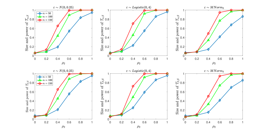
In this section, we evaluate the finite sample performance of and in testing the sparse signal. For this, we set if and otherwise. For simplicity, we set for and for the identification of model (2.1). We choose from When the null hypotheses and hold true. The departure from the null and increases as increases from 0 to 1, while the density of the generated network decreases from to The sample size is set to be and The level is taken as . The critical values are calculated using the bootstrap method with 10000 simulated realizations. For the noise term we consider the following three settings: (i) ; (ii) and (ii) are independently generated from with probability 0.75 and with probability . The corresponding distribution is denoted by All other settings are the same as those in Section 7.1.
Figure 1 shows the empirical size and power of the test statistics and at the significance level 0.05. We observe that the empirical sizes of the proposed tests are close to the nominal level and the tests have reasonable powers to detect deviations from the null hypothesis. The power of the tests increases as increases from to . Also, the powers of the tests increase as increases from to
Next, we evaluate the finite sample performance of the method developed for support recovery. For this, we set and as follows: and where We set and To assess the accuracy of the support recovery, we adopt the following similarity measure (Cai et al., 2013): where with 0 indicating that the intersection of and is an empty set and 1 indicating exact recovery. A high value of indicates that the support recovery is accurate. Table 4 summarizes the mean and the standard deviation of , as well as the numbers of false positives (FP) and false negatives (FN) based on 1000 replications. The results in Table 4 show that tends to approach one as increases. In addition, the values of false positives and false negative are not very high, and decrease as increases.
| Mean | SD | FP | FN | Mean | SD | FP | FN | |||
|---|---|---|---|---|---|---|---|---|---|---|
| 0.978 | 0.057 | 0.229 | 0.281 | 0.977 | 0.056 | 0.264 | 0.264 | |||
| 0.989 | 0.051 | 0.207 | 0.129 | 0.986 | 0.056 | 0.230 | 0.108 | |||
| Logistic(0,4) | 0.977 | 0.062 | 0.377 | 0.263 | 0.979 | 0.060 | 0.317 | 0.255 | ||
| 0.992 | 0.021 | 0.220 | 0.048 | 0.992 | 0.019 | 0.190 | 0.056 | |||
| 0.962 | 0.071 | 0.350 | 0.568 | 0.957 | 0.076 | 0.383 | 0.585 | |||
| 0.984 | 0.064 | 0.262 | 0.241 | 0.983 | 0.059 | 0.233 | 0.224 | |||
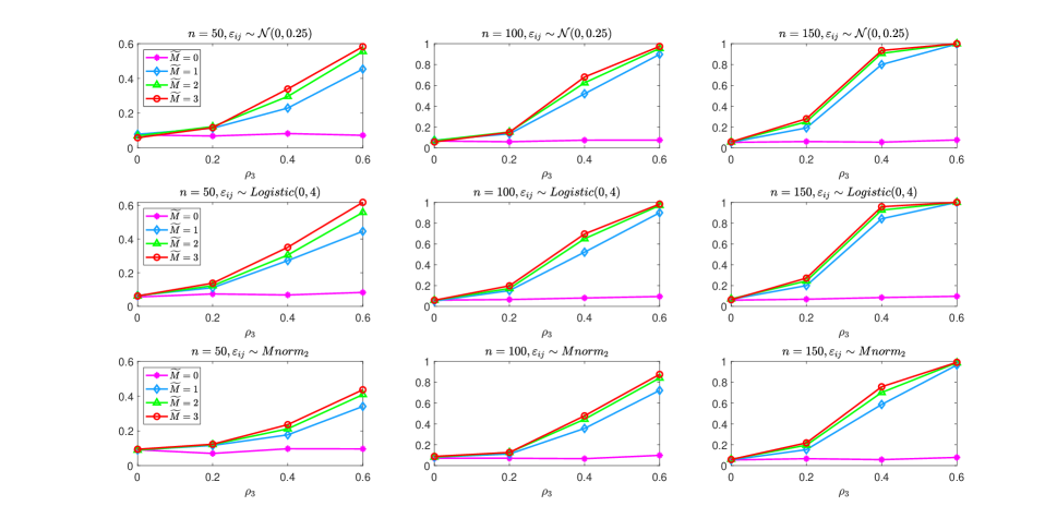
7.3 Testing for degree heterogeneity
In this section, we evaluate the finite sample performance of the tests and in testing the existence of degree heterogeneity. For this, we consider and . Let for for and Under these settings, but Here, we choose and and and Note that and are identical to the tests and respectively, and may not be sensitive to the signals and . In addition, and hold true when The other settings are the same as those used previously.
The results for are summarized in Figure 2. The results for are similar and are omitted here to save space. We see that the empirical sizes of all tests are close to the nominal level However, the test has nearly no power, and hence, fails to detect deviations from the null hypothesis. Figure 2 also suggests that the test with significantly improves the performance of in terms of the power estimation, and the power of increases when increases from to . However, is comparable with Figure S1 in the Supplemental Material shows that the time required to calculate the test may increases with in a linear rate. When and the time required to calculate is approximately 450 seconds for each replication. We also construct simulation studies to evaluate the finite sample performance of the proposed method for the conditionally independent cases and weighted networks. The results are summarized in the section C of the Supplemental Material, which suggest that the proposed method works well.
7.4 Real data analysis
The Lazega¡¯s data of lawyers comes from a network study of corporate law partnership carried out in a Northeastern U.S. corporate law firm between 1988 and 1991 in New England (Lazega, 2001). The data set contains 71 attorneys, including partners and associates of this firm. In the following, we analyze the friendship network among these attorneys, who were asked to name the attorneys whom they socialized with outside of work. In addition, several covariates were collected for each attorney. However, to avoid the curse of dimensionality issue, we only consider the following three covariates: gender (male and female), years with the firm and age, respectively. Prior to our analysis, years with the firm and age are normalized by subtracting the average and dividing by the standard error. As in Yan et al. (2019), we define the covariate for each pair as the absolute difference between the continuous variables and indicators of whether the categorical variables are equal. Since Yan et al. (2019) shows that the effect of age on network formation is significantly negative, we set age as the special regressor and for identification.
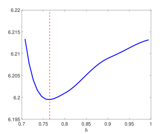
In the data set, individuals are labeled from 1 to 71. After removing the individuals whose in-degrees or out-degrees is zero, we analyze the remaining 63 vertices. We set as the reference. The bandwidth is selected using the procedure developed above, while the kernel is the biweight kernel. As shown in Figure 3, yields the smallest prediction error.
We first conduct the testing procedures outlined in Section 5.1 to assess whether the degree parameters and are equal to zero. The resulting p-values are less than for testing and for testing . This implies that there is degree heterogeneity for both out- and in-degrees at the nominal level . We then apply the support recovery procedure to identify the nonzero signals. The nonzero out-degree parameters are reported in Table 5. Two nodes “11” and “35” have nonzero in-degree parameters with their respective estimates and .
We also implement the procedure described in Section 5.3 to test the existence of degree heterogeneity. The p-values from testing both and are less than 0.001, indicating that the lawyers’ friendship network presents degree heterogeneity.
For homophily effects, the estimated coefficient of gender is 0.112 with confidence interval and the coefficient for years with the firm is -0.219 with confidence interval Thus, the effect of gender on lawyer’s friendship preferences is positive, suggesting that they are more likely to be friend individuals of the same gender. In addition, the effect of years with the firm has a negative effect on network formation, which indicates that the larger the difference between two lawyers¡¯ years with the firm, the less likely they are friends. These results are consistent with the findings reported by Yan et al. (2019).
| ID | CI | ID | CI | ID | CI | |||||
|---|---|---|---|---|---|---|---|---|---|---|
| 1 | 0.641 | 20 | 0.729 | 40 | 1.010 | |||||
| 2 | 0.695 | 22 | 0.872 | 43 | 0.664 | |||||
| 3 | 1.120 | 25 | 0.695 | 45 | 0.864 | |||||
| 8 | 0.839 | 27 | 0.632 | 47 | 0.868 | |||||
| 10 | 1.058 | 29 | 1.043 | 50 | 0.607 | |||||
| 11 | 1.094 | 35 | 1.037 | 56 | 1.493 | |||||
| 12 | 1.052 | 37 | 0.624 | 57 | 1.117 | |||||
| 15 | 1.200 | 38 | 0.748 | 58 | 1.168 | |||||
| 18 | 0.691 | 39 | 0.820 |
8 Conclusions
We propose a semiparametric model for network formation to analyze effects of homophily and degree heterogeneity. The model is flexible in practice because it leaves the distribution of the latent random variables unspecified. We develop a kernel-based least squares method to estimate unknown parameters and derived the asymptotic properties of the estimators, including consistency and asymptotic normal distributions. We present several applications of our general theory, including support recovery, testing for signals and testing the existence of degree heterogeneity.
Several topics need to be addressed in future studies. First, many large-scale network data are very sparse. How to develop the proposed method to analyze large-scale sparse network needs future research. Second, we consider a nonparametric method for the conditional density function of given . It may suffer from the curse of dimensionality, especially when the dimension of is large. Therefore, it is important to develop a dimension reduction procedure before performing the proposed method with high-dimensional data. Finally, the generalization of our methods to analyzing more complicated network data, such as dynamic networks, is also an interesting topic.
Supplemental material
References
- Andrews (1995) Andrews, D. W. (1995). Nonparametric kernel estimation for semiparametric models. Econometric Theory, 11, 560–586.
- Aradillas-Lopez (2012) Aradillas-Lopez, A. (2012). Pairwise-difference estimation of incomplete information games. Journal of Econometrics, 168, 120–140. The Econometrics of Auctions and Games.
- Cai et al. (2013) Cai, T., Liu, W., & Xia, Y. (2013). Two-sample covariance matrix testing and support recovery in high-dimensional and sparse settings. Journal of the American Statistical Association, 108, 265–277.
- Candelaria (2020) Candelaria, L. E. (2020). A semiparametric network formation model with unobserved linear heterogeneity. arXiv preprint arXiv:2203.15603, .
- Chen et al. (2021) Chen, M., Kato, K., & Leng, C. (2021). Analysis of networks via the sparse -model. Journal of the Royal Statistical Society: Series B (Statistical Methodology), 83, 887–910.
- De Paula (2020) De Paula, Á. (2020). Econometric models of network formation. Annual Review of Economics, 12, 775–799.
- Dzemski (2019) Dzemski, A. (2019). An empirical model of dyadic link formation in a network with unobserved heterogeneity. Review of Economics and Statistics, 101, 763–776.
- Fernández-Val & Weidner (2016) Fernández-Val, I., & Weidner, M. (2016). Individual and time effects in nonlinear panel models with large n, t. Journal of Econometrics, 192, 291–312.
- Gao (2020) Gao, W. Y. (2020). Nonparametric identification in index models of link formation. Journal of Econometrics, 215, 399–413.
- Graham (2017) Graham, B. S. (2017). An econometric model of network formation with degree heterogeneity. Econometrica, 85, 1033–1063.
- Graham (2020) Graham, B. S. (2020). Dyadic regression. In The Econometric Analysis of Network Data (pp. 23–40). Academic Press.
- Härdle et al. (1992) Härdle, W., Hart, J., Marron, J. S., & Tsybakov, A. B. (1992). Bandwidth choice for average derivative estimation. Journal of the American Statistical Association, 87, 218–226.
- Honoré & Lewbel (2002) Honoré, B. E., & Lewbel, A. (2002). Semiparametric binary choice panel data models without strictly exogeneous regressors. Econometrica, 70, 2053–2063.
- Hughes (2022) Hughes, D. W. (2022). Estimating nonlinear network data models with fixed effects. arXiv preprint arXiv:2203.15603, .
- Kolaczyk & Csárdi (2014) Kolaczyk, E. D., & Csárdi, G. (2014). Statistical Analysis of Network Data with R. Springer.
- Lazega (2001) Lazega, E. (2001). The collegial phenomenon: The social mechanisms of cooperation among peers in a corporate law partnership. Oxford University Press, USA.
- Lewbel (1998) Lewbel, A. (1998). Semiparametric latent variable model estimation with endogenous or mismeasured regressors. Econometrica, 66, 105–121.
- Lewbel (2000) Lewbel, A. (2000). Semiparametric qualitative response model estimation with unknown heteroscedasticity or instrumental variables. Journal of Econometrics, 97, 145–177.
- Manski (1985) Manski, C. F. (1985). Semiparametric analysis of discrete response: Asymptotic properties of the maximum score estimator. Journal of Econometrics, 27, 313–333.
- Nadaraya (1964) Nadaraya, E. A. (1964). On estimating regression. Theory of Probability & Its Applications, 9, 141–142.
- Neyman & Scott (1948) Neyman, J., & Scott, E. L. (1948). Consistent estimates based on partially consistent observations. Econometrica, 16, 1–32.
- Qi et al. (2005) Qi, L., Wang, C. Y., & Prentice, R. L. (2005). Weighted estimators for proportional hazards regression with missing covariates. Journal of the American Statistical Association, 100, 1250–1263.
- Stein & Leng (2023) Stein, S., & Leng, C. (2023). An annotated graph model with differential degree heterogeneity for directed networks. Journal of Machine Learning Research, 24, 1–69.
- Toth (2017) Toth, P. (2017). Semiparametric estimation in network formation models with homophily and degree heterogeneity. Working paper, Available at SSRN 2988698, 1–81.
- Watson (1964) Watson, G. S. (1964). Smooth regression analysis. Sankhyā: The Indian Journal of Statistics, Series A, (pp. 359–372).
- Yan et al. (2019) Yan, T., Jiang, B., Fienberg, S. E., & Leng, C. (2019). Statistical inference in a directed network model with covariates. Journal of the American Statistical Association, 114, 857–868.
- Zeleneev (2020) Zeleneev, A. (2020). Identification and estimation of network models with nonparametric unobserved heterogeneity. Working paper, Department of Economics, Princeton University.