Simple and explicit constructions of semi-discrete surfaces and discrete surfaces
Abstract.
We give a simple and explicit constructions of various semi-discrete surfaces and discrete -surfaces in terms of the Jacobi elliptic functions using -functions. Their periodicities are also determined.
Introduction
The discrete sine-Gordon equation was introduced by R. Hirota([2]). After that, as an application of discrete sine-Gordon equation to the discrete differential geometry, significant progress was done by Bobenko-Pinkall in [1]. They gave the solution of discrete sine-Gordon equation in terms of the Riemann theta function and gave a formulae for the immersion of the discrete -surface. On one hand, the industrial mathematics researchers has been studying the discrete space curve and the isoperimetric deformation of the discrete space curve (for example, see [3],[4]), of which the integrability is given by the semi-discrete sine-Gordon equation. The theory of discrete space curves have recently attracted attention as equations of motion that describe the Kaleidocycle(see [4], [5]). The Kaleidocycle is demonstrated by a deformation of a discrete space curve which is periodic with respect to the integer parameter. Very recently, some examples of the Kaleidocycle are given in [5] and they are described in terms of the Jacobi theta functions. On the other hand, in [7], we gave solutions in terms of the Jacobi elliptic functions for both the discrete and semi-discrete sine-Gordon equations. They are said to be “dn-solution”because the cosine of the solution function may be described in terms of the Jacobi dn-function. In fact, although the solution in terms of Riemann theta function has been given in [1], it is not so clear to deduce the elliptic function solution from that. It is because the Riemann period matrix is differeent from the ordinary form and the expressions using Riemann theta function for the Jacobi elliptic functions are different from the ordinary one. For this problem, in [7], we investigate the spectral curve for the sine-Godron equation and obtain a Weierstrass -function and determined the two periods of it, which teachs one how the form of the Riemann period matrix is. This knowledge made it possible to clarify the relationship between the elliptic solution and the Riemann theta function solution (see [7]). Based on these observations, we may find -functions for constructing semi-discrete surface (for the definition, see the preliminaries) which correspond to the Baker-Akhiezer functions in the theory of Bobenko-Pinkall([1]).
In this paper, first of all, we shall give several definitions of the discrete objects which we are interested in. Next, we give “cn-solution”of the semi-discrete and discrete sine-Gordon equations, that is, the cosine of the solution function may be described in terms of the Jacobi cn-function, which are done in §1 and §2. In §3, we shall give a general method of construction of semi-discrete surface in terms of -functions. In §4, we shall give the -functions which are described in terms of the ceratin Jacobi theta functions and give interesting examples of the semi-discrete surfaces which corresponds to the -solution of the semi-discrete SG-equation. In §5, choosing another -functions which are described in terms of the certain Jacobi theta functions, we give another example of the semi-discrete surface which corresponds to the -solution of the semi-discrete SG-equation. Some periodic solutions among the examples constructed in §4 and §5 yield the model of the Kaleidocycle. In §6, we shall give interesting examples of discrete -surfaces in the sense of [1] using the results in §4 and §5. §7 is Appendix, which is devoted to demonstrate the well-known properties of Jacobi theta functions and the properties of the elliptic functions needed in §1§5.
Preliminaries
First of all, we shall give the several difinition of discrete objects which we are interested in.
Definition 0.1.
(1) A map is said to be a discrete space curve if for any and any consecutive three points and are not collinear.
(2) A map is said to be a semi-discrete surface if is a deformation of the discrete space curve with the deformation parameter .
(3) A map is said to be discrete K-surface if (i) every point and its neighbours belong to one plane , (ii) the lengths of the opposite edges of an elementary quadrilateral are equal
where does not depend on and not on .
The definition of the discrete -surface is due to Bobenko-Pinkall ([1]). For a while from now, we are constrate on the semi-discrete surface with the deformation parameter . We may construct a Frenet frame associated to as follows. Define by , where . Choose so that for some constant for each . We assume that has constant speed. We then see that is constant and independent of , which we denote by just . Finally, we define by . The signed curvature and the torsion angle is defined by
If we set , we obtain , where
| (0.3) |
(see [3], [4]). Moreover, we assume that is constant and independent of , which we denote by just . Under this situation, the deformation is said to be isoperimetric if there is some constant , which is independent of , and some function such that the following holds.
| (0.4) |
Then, we obtain (see [4]). In the case of , and are controlled by the solution of the semi-discrete SG-equation. On the other hand, in the case of , and are controlled by the solution of the semi-discrete potential mKdV-equation (see Remark 2 in [4]). However, since our solution below to the semi-discrete SG-equation satisfies also the potential mKdV-equation (see §1), our solution covers both cases of the relations between and .
To obtain the Weierstrass -function stated in the introduction, we consider the spectral curve for the smooth SG-equation. For a function of the parameters and , the smooth SG-equation is given by , where . Set and assume that , a function which depends on only parameter . We then rewrite the SG-equation as . Multiplying it by and integrating it, we obtain
where is an integration constant and determined by an initial condition. We give the initial condition by , where is the modulus of the Jacobi dn-function because is a -solution of the smooth SG-equation. By the initial condition, we see that . If we set , we then obtain . If we set , we then have
where , and . This is a standard form of the elliptic curve and parametrized by , where is a Weierstrass -function. We may express it in terms of the Jacobi elliptic functions as follows.
Lemma 0.5.
([7])
| (0.6) |
We find by (0.6) that the two periods of are given by
| (0.7) |
The holomorphic 1-form and the normalized abelian differential of second kind on the spectral elliptic curve are given by
| (0.8) |
where is the Weierstrass -function (see [7]).
1. Solutions of semi-discrete sine-Gordon equation in terms of the Jacobi elliptic function
In [7], it is proved that is a solution of the semi-discrete sine-Gordon equation
where with some constants , and is given by
Moreover, also satisfies the mKdv equation
where
Since we may write as , we call this solution “dn-solution”. We here prove that there is also “cn-solution ”for the sine-Gordon equation. For this, we take and and consider . We then calculate using (i) of Lemma 7.1 as follows.
Therefore, we have . Then, by the similar calculation as in [7] we see that satisfies the semi-discrete sine-Gordon equation for replaced by . It also satisfies the mKdV equation for replaced by .
2. Solutions of discrete sine-Gordon equation in terms of the Jacobi elliptic functions
Set . In [7], it is proved that is a solution of the discrete sine-Gordon equation
| (2.3) |
where
for a solution . Since we may write , this solution is called “-solution. Next, we search for the “-solution. For this, set
We consider . Setting , we calculate using (i) of Lemma 7.1, we obtain the following.
and
Now, we see that
Since we have
we obtain the following.
Therefore, we see that , which is a “- solution”.
3. Construction of semi-discrete surface
Given a solution of the semi-discrete sine-Gordon equation,we write it as . After choosing such , we consider the unitary frame defined by
where and all the functions in the entries are functions of some parameters and . Setting , we write the component of as . We use an isomorphism defined by
where . We choose some so that . Set
Hereafter, we write as and so on.
We then express a vector as
| (3.1) |
where
| (3.4) |
For a nonnegative integer , we introduce functions satisfying following relations.
| (3.13) |
where the imaginary unit, and and is the Hirota differetiation operator with a real parameter and , respectively. Moreover, we assume that the following relations hold.
| (3.18) |
With these solutions we obtain semi-discrete surface . We may define a Frenet frame associated to . Set and . When , we define the frame as follows.
| (3.22) |
We write , where corresponds to in (0.3). We find as follows.
Lemma 3.23.
For , we have the following.
(2) .
Proof. (1) We show . For this purpose, we calculate and and obtain the following.
Using , we then have the following.
(2) First note that , where . We then have
Therefore, we have . ∎
Alternatively, when , we define the frame as follows.
| (3.30) |
We write . We then have the following.
Lemma 3.31.
For , we have the following.
(2) .
Theorem 3.32.
After choosing which satisfies for a solution of the semi-discrete sine-Gordon equation, under the conditions (3.1)(3.4), we obtain the following.
| (3.33) |
Moreover, we have .
Proof. The form of follows from (3.1), (3.2), first two equations in (3.3) and (3.4). The form of easily follows from its definition (3.5)(or (3.7)). We calculate , then we find the following using the last four equations of ( LABEL:fgFH).
It follows from (2) of Lemma 3.23 that we may define and by
∎
We give here the example of . We consider the following Weierstrass -function stated in (0.6) :
where and . The two periods of are given by and . In particular, we see that . Let be the Weierstrass -function. We define by
| (3.35) |
where is a function of and is some real-valued function which depends only and , which is determined explicitly later. Moreover, we choose so that the integration part in the is real-valued.
4. Semi-discrete surfaces corresponding to -solution”of semi-discrete SG-equation
We construct a semi-discrete space curve which corresponds to the solution of the semi-discrete SG-equation. Set
where is a real-valued function of some parameters, is the complete elliptic integral of 1st kind with modulus and for . We then see that for real parameters and . In this case, we may verify the following.
| (4.4) |
where and .
We choose in this section. Set
Lemma 4.5.
Set and . We choose -functions as follows.
We then have , hence is a “dn-solution”. We may verify that these functions satisfy (3.3) and (3.4) for .
Proof. Let be a “dn- solution”. For , we take and ,which yield . Since and , we have . On the other hand,
where we have used Lemma 7.4, Lemma 7.6 and . For ,we use the fourth equation of Lemma 7.4 for .
For , considering (3.4) we calculate as follows.
The rest two equations in (4.3) are prepared to ensure that . Therefore, we prove them in the proof of the next Theorem. ∎
Theorem 4.10.
where and . We have also the following properties.
(i) , thus and . The compound sign is in the same order as the compound sign in (3.22).
(ii) , and .
(iii) is an isoperimetric deformation of the discrete space curve, that is, the following holds. , where .
Proof. First, we rewrite .
where we have used the first and second equations of Lemma 7.4 for . We here calculate the reciprocal of the expression in parentheses.
where we have used and Lemma 7.6. Therefore, we obtain the following.
and
| (4.13) |
We denote by the -th component of for . Now, we see that
Lastly, we calculate the third component .
Here we point out the following is known.
We apply this formulae to our case by taking . We then see that
We then have
where we used the Legendre equation in the second equality to the last. Thus, we obtain the following.
| (4.17) |
On the other hand, when we take in (3.35), we have from (ii) of Lemma 7.4,
| (4.22) |
It follows from (4.5) and (4.6) that
Next, we show using (3.6). Set and . We write . We first calculate .
which implies that
Therefore, we see that
Finally, to obtain the third component of we calculate .
which, together with (ii) of Lemma 7.6, yields
Next, we prove that . For this, we calculate in the same way and obtain the following.
| (4.26) |
On the other hand, it follows from (4.4) that
| (4.27) |
Using the assumption and comparing (4.7) and (4.8), we see from (iv) and (v) of Lemma 7.12 that
which implies that for . The third component of is given by
On the other hand, is given by
To show the equality , first we show that the derivations by of both equations coincide. We must have the following equation.
which, together with the equation multiplying (iv) of Lemma 7.12 by , yields
The last equation is equivalent to (vi) of Lemma 7.12. Therefore, we see that there is a function such that
Setting in the equation above, we easily see that dose not depend on . Therefore, we see that , hence we are done. Now, we show the rest properties of and . follows from (i) of Lemma 7.12. Using and (iv) of Lemma 7.12, we obtain
We consider the case where the sign in the definition (3.22) is “”. In this case, we choose so that . Since , divide it by we have and as follows.
which are compatible with the definition (3.22). For this, we use the following.
We then see that , which also follows from (iii) of Lemma 7.12 directly. For the case where the sign in the definition (3.22) is “”, we choose so that and define by . We then have . Under the condition , to calculate we use (v) and (iv) of Lemma 7.12.
Therefore, we see that . Finally, calculating the differential of by , we have
which implies that and
∎
Similarly, in Lemma 4.2, we change by .
Lemma 4.34.
We choose -functions as follows.
These satisfy (3.3) and (3.4) for . In this case, we have . We then have the following.
Corollary 4.36.
where and . We have also the following properties.
(i) , thus and . The compound sign is in the same order as the compound sign in (3.30).
(ii) , and .
(iii) is an isoperimetric deformation of the discrete space curve, that is, the following holds. , where .
Proof. We just show the properties. follows from (i) of Lemma 7.12. We consider the case where the sign in the definition (3.30) is “”. In this case, we choose so that . Since , we define and by and . We then have
which are compatible with the definition (3.30). We may calculate as in the proof of Theorem 4.10 and find that . Moreover, we then see that . For the case where the sign in (3.30) is “”, we choose so that and define by . We then see that . Finally, is given by
which implies that
∎
[Periodicity] Assume that and in . The torsion is given by . In this case, we have . Since , we see that
Therefore, the third element of is independent of . It follows from that is also independent of . For and , these are periodic if or according as or . This is possible when we choose so that . Thus, for arbitrary , there is a such that holds for any .
5. Semi-discrete surfaces corresponding to “-solution”of semi-discrete SG-equation
We construct a semi-discrete space curve which corresponds to the solution of the semi-discrete SG-equation. Set
| (5.8) |
We then see that and . In this case, we may verify the following.
| (5.12) |
For , the same equations hold as above.
Lemma 5.13.
Set and . We choose -functions as follows.
We then have , hence is a “cn-solution”. We may verify that these functions satisfy (3.3) and (3.4) for .
Proof. Let be a “cn-solution”. Then, for the same choice of as that in the proof of Lemma 4.2 except for the chice of , we have and . On the other hand,
where we have used Lemma 7.4 and Lemma 7.6. For ,we use the fourth equation of Lemma 7.4 for .
where . For , considering (3.4) we calculate as follows.
The rest two equations in (3.3) are prepared to ensure that . Therefore, we prove them in the proof of the next Theorem. ∎
We then have the following.
Theorem 5.18.
where and . We have also the following properties.
(i) , thus and . The compound sign is in the same order as the compound sign in (3.22).
(ii) , and .
(iii) is an isoperimetric deformation of the discrete space curve, that is, the following holds. , where .
Proof. Sinec the essential part of the proof is almost same as that of Theorem 4.10, we here present the outline.
Therefore, we obtain the following.
and
| (5.20) |
We then see that and . For , the calculation is alomost same as that of Theorem 4.3. The only difference is to take . Next, we prove that . For this, we calculate in the same way and obtain the following.
| (5.21) |
On the other hand, it follows from (5.5) that
| (5.22) |
Using the assumption and comparing (5.6) and (5.7), we see from (vii) and (viii) of Lemma 7.12 that
which implies that for . The proof for is same as that of Theorem 4.3. The rest properties of and are easily verified by direct calculations. We consider the case where the sign in the definition (3.22) is “”. In this case, we choose so that . Since , divide it by we have and as follows.
which are compatible with the definition (3.22). We then see that . For the case where the sign in the definition (3.22) is “”, we choose so that and define by . We then see that . For , we calculate using (v) and (iv) of Lemma 7.12.
Threfore, we see that . ∎
Similarly, in Lemma 5.3, we change by .
Lemma 5.25.
We choose -functions as follows.
We then have the following.
Corollary 5.27.
where and . We have also the following properties.
(i) , thus and . The compound sign is in the same order as the compound sign in (3.30).
(ii) , and .
(iii) is an isoperimetric deformation of the discrete space curve, that is, the following holds. , where .
Proof. The main part of the proof is almost same as that of Theorem 5.18. We consider the case where the sign in the definition 3.30 is “”. Since we have , we choose so that . We define and by and . We then have
which are compatible with the definition 3.30. We then see that . For the case where the sign in the definition 3.30 is “”, we choose so that and define by . We then see that . Moreover, is given by
In the same way as the proof of Theorem 5.18, we may prove the rest properties. ∎
[Periodicity] Assume that and in . The third element of is independent of as in §4. The torsion is given by . In this case, we have , that is, . Since we know that
we have holds for any .
6. Discrete -surfaces corresponding to - solution or -solution of the discrete sine-Gordon equation
As an application of the results in and , we may construct a discrete -surface in the sense of Bobenko-Pinkall([1]). In [1], a general formulae in terms of the Riemann theta functions for the immersion of discrete -surface is obtained using the theory of the spectral curve and the Baker-Akhiezer function. However, when one try to produce a non-trivial concrete example of the discrete -surface using their formulae, it is difficult to use the formulae directly. Therefore, it is realistic to limit the genus of the spectral curve to 1. In this point of view, we may use the results obtained in and . For a discrete -surface , first we construct the unitary frame associated to . We write
| (6.1) |
Referring to the unitary frames and in Lemma 3.23 and Lemma 3.31, respectively, we choose and as follows.
| (6.5) |
However, these does not satisfy the compatibility condition for the translation . As in [1], we use the gauge transformation . We then see that and are transformed to and , respectively. We choose ’s as follows.
We then have the following.
| (6.9) |
For the compatibility condition , we have the following.
Proposition 6.10.
(1) holds if and only if is a solution of the discrete sine-Gordon equation with .
(2) holds if and only if is a solution of the discrete sine-Gordon equation with .
Proof. We prove the case (1) only. The case (2) is similarily proved. For simplicity of the notation, we use the following abbreviation.
We then see that holds if and only if
which is equivalent to
which is also equivalent to
For , we have . Thus, the last equation is equivalent to
which is again equivalent to , which is the discrete sine-Gordon equation stated in §2 for . For example, for “dn-solution”, . For “cn-solution”, . For this, just use and each values and in “dn-solution”or “cn-solution”. ∎
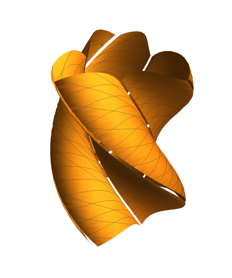
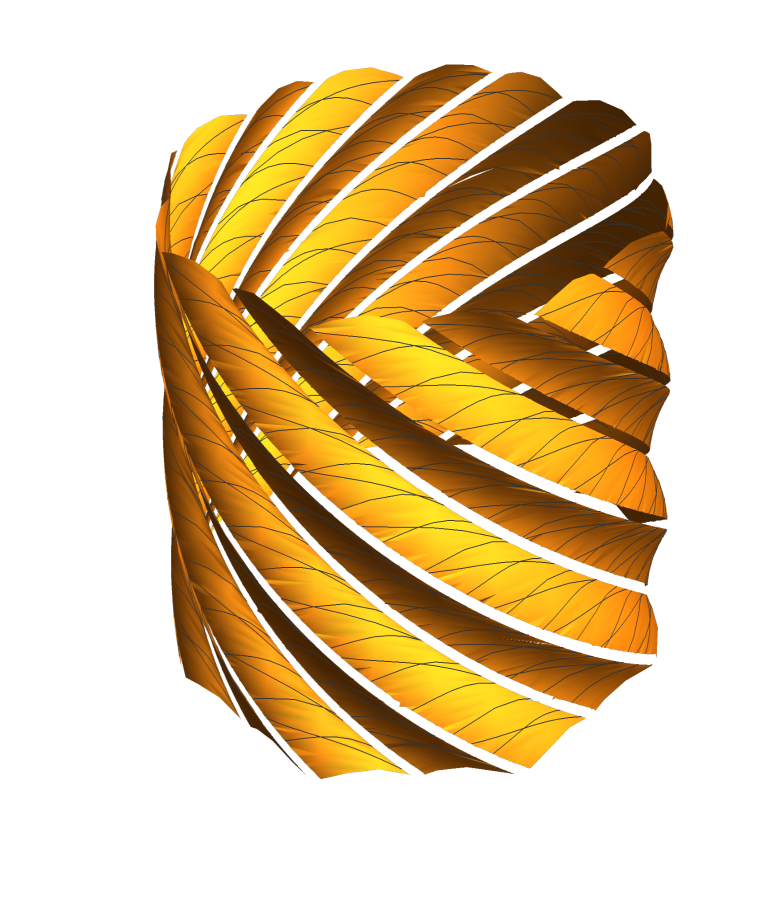
The following is an example of discrete -surface corresponding to the “dn-solution”of the discrete sine-Gordon equation.
Theorem 6.12.
The following gives a discrete -surface.
| (6.13) |
where with . Moreover, we have the following properties.
(i) ,
(ii) , where
| (6.14) |
Proof. The form of follows from Theorem 4.10 and Corollary 4.36, where we write ’s as . Therefore, we see that the properties (i) and (ii) hold. We then see that both of and are perpendicular to . Hence, there is a plane such that three points lies on . However, since we also have and , the rest two points and also lies on . Thus, is a discrete -surface. ∎
For in Theorem 6.12, while corresponds to the curvature , corresponds to the curvature .
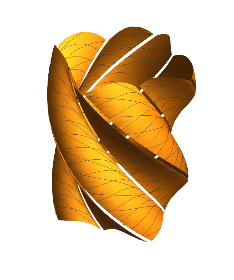
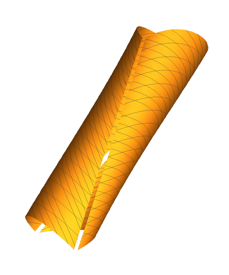
The next example of a discrete -surface corresponds to the “cn-solution”of the discrete sine-Gordon equation.
We have the following theorem.
Theorem 6.15.
The following gives a discrete -surface.
| (6.16) |
where with . Moreover, we have the following properties.
(i) ,
(ii) , where
| (6.17) |
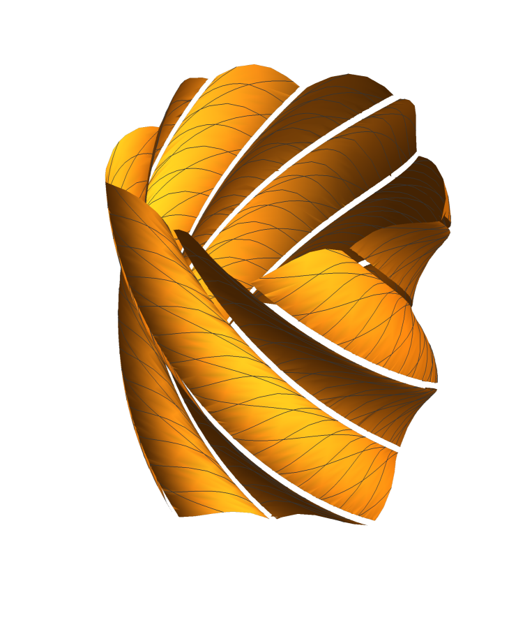
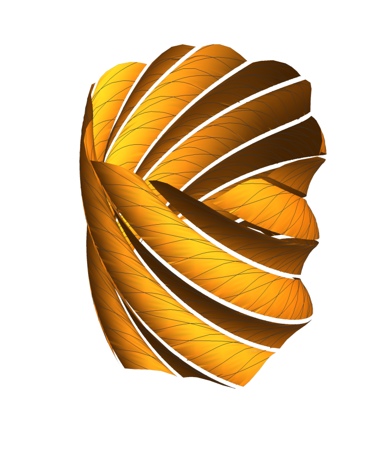
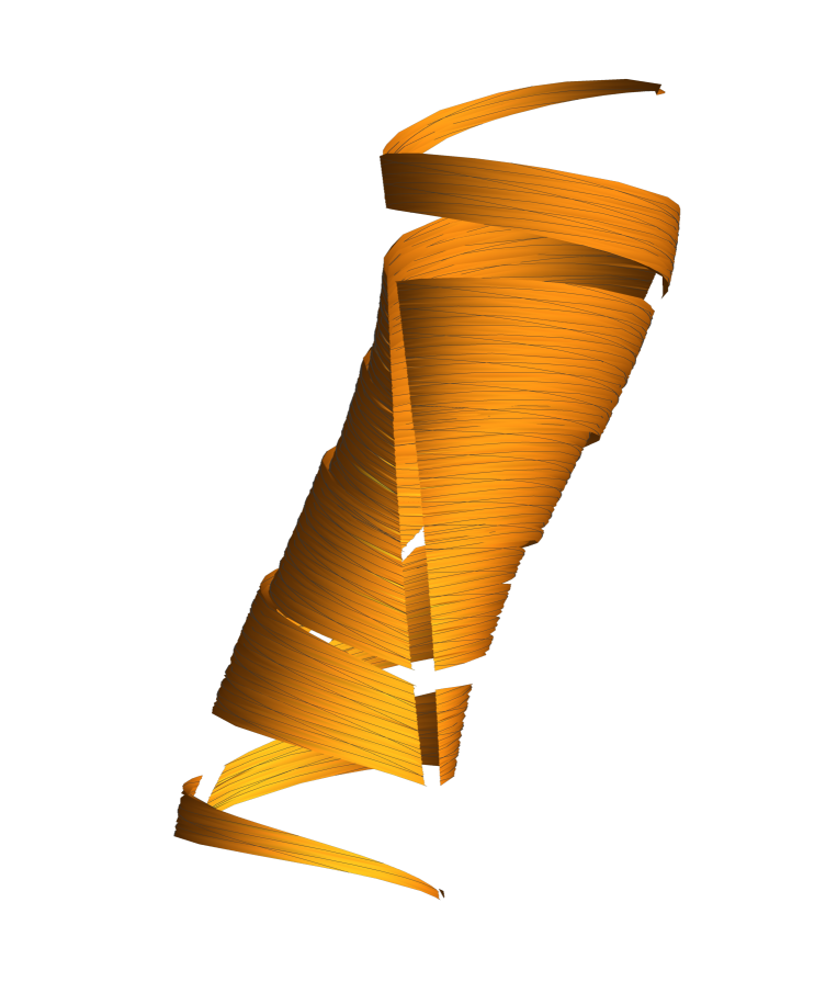
[Periodicity]
-
(1)
For , we may utilize the arguments of the periodicity in §4.
-
(a)
The case of . Assume that and , where . Since and , we must have and , thus we have . Choosing so that for any with . We then see that for any and any .
-
(b)
The case of . In this case, , hence . Let be the same one as in (i). We see that for any .
-
(c)
The case of means .
-
(a)
-
(2)
For , we may utilize the arguments of the periodicity in §5.
-
(a)
The case of . In this case, we have . We then have and . We see that and for any .
-
(b)
The case of . We then have and . We see that and for any .
-
(c)
The case of . We then have and . We see that and for any .
-
(a)
7. Appendix
The following formulae are well known.
Lemma 7.1.
Using Lemma 7.1 and considering the cases of or , we obtain the following.
Lemma 7.4.
For , we have
Lemma 7.6.
Let and .
(i) , (ii) ,
(iii) .
The Weierstrass -function defined in (0.4) has two periods and . Remark that .
Lemma 7.7.
Let be the Weierstrass -function satisfying . We then have
(i) , (ii) .
Proof. (i) Use the following formulae.
It follows from (0.4) that , where . Therefore, we see that
which, together with the formulae above for , implies the result (i). For (ii), first note that . We calculate the integral
On the other hand, we have , which together with the Legendre identity , and the above, implies that
| (7.10) |
which ,together with result (i), yields that
Therefore, from the Legendre formulae we have
| (7.11) |
On the other hand, we see that
Therefore, we have the result (ii). ∎
Lemma 7.12.
For , the following equations hold identically.
(i) ,
(ii) ,
(iii) ,
(iv) ,
(v) ,
(vi)
(vii) ,
(viii) ,
(ix)
Proof. These equations hold because of and the addition formulae for and -functions of the following.
For , replace by in the equations above. ∎
References
- [1] A. Bobenko and U. Pinkall, Discrete surfaces with constant negative Gaussian curvature and the Hirota equation, Journal of Differential Geometry 43(1996), no.3, 527-611.
- [2] R. Hirota, Nonlinear partial difference equations III discrete sine-Gordon equation, J. Phys. Soc. Japan 43,1977, 2079-2086.
- [3] J. Inoguchi, K. Kajiwara, N. Matsuura and Y. Ohta, Discrete mKdV and discrete sine-Gordon flows on discrete space curves, J. Physics A: Math. Theor. 47, 2014, 235202.
- [4] S. Kaji, K. Kajiwara and H. Park, Linkage mechanisms governed by integrable deformations of discrete space curves, Nonlinear Systems and Their Remarkable Mathematical Structures: Volume 2 (CRC Press,2019),356-381.
- [5] S. Kaji, K. Kajiwara and S. Shigetomi, An explicit construction of Kaleidocycles, a preprint.
- [6] K. Sogo, Variational discretization of Euler’s elastica problem, J. Phys. Soc. Japan 75, 2006, 064007.
- [7] S. Udagawa, K. Kajiwara and J. Inoguchi. Solutions of sine-Gordon equation and its discretization(written in Japanese), Bull. Liberal Arts and Sciences, Nihon Univ. School of Medicine, no. 50, 2022, 6-26.
- [8] NIST, Digital Library of Mathematical FUnctions, https://dlmf.nist.gov/