On the closure of curvature in 2D flamelet theory

Hernan Olguin Corresponding author
Email address: hernan.olguin@usm.cl Department of Mechanical Engineering, Universidad Técnica Federico Santa María,Avenida España 1680, Valparaíso, Chile
Pascale Domingo CORIA CNRS, Normandie Université, INSA de Rouen, Technopôle du Madrillet, BP 8,Saint-Étienne-du-Rouvray 76801, France Luc Vervisch CORIA CNRS, Normandie Université, INSA de Rouen, Technopôle du Madrillet, BP 8,Saint-Étienne-du-Rouvray 76801, France Christian Hasse Institute for Simulation of reactive Thermo-Fluid Systems, TU Darmstadt,Otto-Berndt-Straße 2, 64287 Darmstadt, Germany Arne Scholtissek Institute for Simulation of reactive Thermo-Fluid Systems, TU Darmstadt,Otto-Berndt-Straße 2, 64287 Darmstadt, Germany
Abstract

So far, flamelet theory has treated curvature as an independent parameter requiring specific means for closure. In this work, it is shown how the adoption of a two-dimensional orthogonal composition space allows obtaining formal mathematical relations between the flame curvatures and the gradients of the conditioning scalars (also called flamelet coordinates). With these, both curvatures become a flame response to the underlying flow, which conveniently allows removing them from the corresponding set of flamelet equations. While the demonstration is performed in the context of partially premixed flames, the approach is general and applicable to any orthogonal coordinate system.

1 Introduction

Orthogonal coordinate systems have been recently proposed as an ideal framework for the derivation of flamelet equations for partially premixed flames: Their adoption avoids the need of closure means for the cross scalar dissipation rate and leads to a formulation allowing for a direct recovery of the asymptotic limits of non-premixed and premixed combustion [1, 2]. In this context, it has been shown how, after introducing the mixture fraction, $Z$, as main coordinate, a modified reaction progress variable, $\varphi$, can be defined in such a way that it satisfies the orthogonality condition, $\nabla Z\cdot\nabla\varphi=0~{}$[2]. Based on the ($Z,\varphi$)-space, flamelet equations for the chemical species mass fraction, temperature, and both conditioning scalar gradients, $g_{Z}=\lvert\nabla Z\rvert$ and $g_{\varphi}=\lvert\nabla\varphi\rvert$, have been obtained in terms of four parameters: Two strain rates and two curvatures.

Classical combustion theory naturally contains strain and curvature components, such that the latter is often considered a parameter, rather than a flame response (see for example [3, 4, 5]). Similarly, flamelet theory has so far treated flame curvatures as independent parameters [6, 7, 8, 9]. However, it will be shown now that the adoption of an orthogonal coordinate system has an additional yet unexplored advantage, namely the fact that it allows connecting the curvatures with the derivatives of the scalar gradients, $g_{Z}$ and $g_{\varphi}$. With this, the two strain rates are the only parameters remaining in the formulation proposed in [2], while curvature becomes a flame response to the underlying flow.

2 The relation between the curvatures and the conditioning scalar gradients

We start the derivation considering a flamelet-like transformation from a two-dimensional physical space, ($t,x,y$) into a corresponding composition space, ($\tau,Z,\varphi$). Here, $\tau$ is a time-like variable and the mixture fraction, $Z$, and the modified reaction progress variable, $\varphi$, are formally defined through their respective governing equations

$$\frac{\partial Z}{\partial t}+\mathbf{u}\cdot\nabla Z=\frac{1}{\rho}\nabla\cdot\left(\rho D\nabla Z\right)$$ (1)

and

$$\frac{\partial\varphi}{\partial t}+\mathbf{u}\cdot\nabla\varphi=\frac{1}{\rho}\nabla\cdot\left(\rho D\nabla\varphi\right)+\frac{\dot{\omega}_{\varphi}}{\rho},$$ (2)

where $\mathbf{u}$ is the flow velocity, $\rho$ denotes the gas density and $D$ corresponds to a diffusion coefficient. Moreover, the source term in Eq. (2) is defined as

$$\dot{\omega}_{\varphi}=\dot{\omega}_{c}+\rho D\lvert\nabla Z\rvert^{2}\frac{\partial^{2}Y_{c}}{\partial Z^{2}},$$ (3)

where the conventional reaction progress variable, $Y_{c}$, is defined as a suitable combination of (product) species mass fractions. With Eq. (3), it is ensured that the orthogonality condition, $\nabla Z\cdot\nabla\varphi=0$, is satisfied (see formal derivation in [2]).

Based on $Z$ and $\varphi$, two unit vectors can be introduced now as

$$\mathbf{n}_{Z}=\frac{\nabla Z}{\lvert\nabla Z\rvert}~{}\text{ }~{}\text{ and }~{}\text{ }~{}\mathbf{n}_{\varphi}=\frac{\nabla\varphi}{\lvert\nabla\varphi\rvert},$$ (4)

which allows defining the two associated curvatures

$$\kappa_{Z}=-\nabla\cdot\mathbf{n}_{Z}~{}\text{ }~{}\text{ and }~{}\text{ }~{}\kappa_{\varphi}=-\nabla\cdot\mathbf{n}_{\varphi}.$$ (5)

For simplicity, in the rest of this section we will focus on $\kappa_{\varphi}$ and its relation with $g_{Z}=\lvert\nabla Z\rvert$, but the analysis can be replicated to study the relation between $\kappa_{Z}$ and $g_{\varphi}=\lvert\nabla\varphi\rvert$.

Now, the orthogonality between $\mathbf{n}_{Z}$ and $\mathbf{n}_{\varphi}$ allows relating the components of these two vectors. For example, expressing them in the following generic form

$$\mathbf{n}_{Z}=n_{x}\mathbf{e}_{x}+n_{y}\mathbf{e}_{y}~{}\text{ }~{}\text{ and }~{}\text{ }~{}\mathbf{n}_{\varphi}=m_{x}\mathbf{e}_{x}+m_{y}\mathbf{e}_{y},$$ (6)

where $\mathbf{e}_{x}=(1,0)^{T}$ and $\mathbf{e}_{y}=(0,1)^{T}$, it is clear that the required orthogonality can be satisfied setting $m_{x}=n_{y}$ and $m_{y}=-n_{x}$, since

$$(\mathbf{n}_{Z}\cdot\mathbf{n}_{\varphi})=n_{x}n_{y}-n_{y}n_{x}=0.$$ (7)

With this, $\kappa_{\varphi}$ can be rewritten as

$$\kappa_{\varphi}=-\frac{\partial n_{y}}{\partial x}+\frac{\partial n_{x}}{\partial y},$$ (8)

where the derivatives at the RHS correspond to different components of the curvature tensor, $\nabla\mathbf{n}_{Z}$. These can be further worked out in terms of $Z$ by means of the following identity [10] (see Appendix A for a detailed derivation)

$$\frac{\partial n_{i}}{\partial x_{j}}=\frac{1}{g_{Z}}\left[\frac{\partial^{2}Z}{\partial x_{i}\partial x_{j}}-n_{i}n_{k}\frac{\partial^{2}Z}{\partial x_{j}x_{k}}\right],$$ (9)

which yields

$$\frac{\partial n_{y}}{\partial x}=\frac{1}{g_{Z}}\left[\frac{\partial^{2}Z}{\partial x\partial y}-n_{x}n_{y}\frac{\partial^{2}Z}{\partial x^{2}}-n_{y}^{2}\frac{\partial^{2}Z}{\partial x\partial y}\right]$$ (10)

and

$$\frac{\partial n_{x}}{\partial y}=\frac{1}{g_{Z}}\left[\frac{\partial^{2}Z}{\partial x\partial y}-n_{x}^{2}\frac{\partial^{2}Z}{\partial x\partial y}-n_{x}n_{y}\frac{\partial^{2}Z}{\partial y^{2}}\right],$$ (11)

respectively. Replacing back in Eq. (8), we obtain

$$\kappa_{\varphi}=\frac{1}{g_{Z}}\left[n_{x}n_{y}\left(\frac{\partial^{2}Z}{\partial x^{2}}-\frac{\partial^{2}Z}{\partial y^{2}}\right)+\left(n_{y}^{2}-n_{x}^{2}\right)\frac{\partial^{2}Z}{\partial x\partial y}\right],$$ (12)

where the term in brackets at the RHS of this equation corresponds to $\partial g_{Z}/\partial n_{\varphi}=g_{\varphi}\partial g_{Z}/\partial\varphi$, as it will be shown next.

Based on the definition of the directional derivative, we can write

$$\frac{\partial g_{Z}}{\partial n_{\varphi}}=\mathbf{n}_{\varphi}\cdot\nabla g_{Z}=n_{y}\frac{\partial g_{Z}}{\partial x}-n_{x}\frac{\partial g_{Z}}{\partial y},$$ (13)

where the derivatives at the RHS can be further worked out by means of the following mathematical identity (see Appendix A for a detailed derivation)

$$\frac{\partial g_{Z}}{\partial x_{j}}=n_{i}\frac{\partial^{2}Z}{\partial x_{i}\partial x_{j}},$$ (14)

which yields

$$\frac{\partial g_{Z}}{\partial x}=n_{x}\frac{\partial^{2}Z}{\partial x^{2}}+n_{y}\frac{\partial^{2}Z}{\partial x\partial y}$$ (15)

and

$$\frac{\partial g_{Z}}{\partial y}=n_{x}\frac{\partial^{2}Z}{\partial x\partial y}+n_{y}\frac{\partial^{2}Z}{\partial y^{2}},$$ (16)

respectively. Replacing in Eq. (13), we have

$$\frac{\partial g_{Z}}{\partial n_{\varphi}}=n_{x}n_{y}\left(\frac{\partial^{2}Z}{\partial x^{2}}-\frac{\partial^{2}Z}{\partial y^{2}}\right)+\left(n_{y}^{2}-n_{x}^{2}\right)\frac{\partial^{2}Z}{\partial x\partial y},$$ (17)

which can be inserted in Eq. (12) to obtain

$$\kappa_{\varphi}=\frac{g_{\varphi}}{g_{Z}}\frac{\partial g_{Z}}{\partial\varphi},$$ (18)

which, together with its equivalent expression for $\kappa_{Z}$, will allow removing both curvatures as parameters in the corresponding flamelet equations, as it will be shown in Section 4.

At this point, two important aspects must be highlighted. First, the derivation shown in this section is not the only possible path to obtain Eq. (18) (see for example Appendix B for an alternative derivation). Secondly, it is interesting that Eq. (18) can be recast as one of the terms appearing in the multi-dimensional flamelet equation obtained in [11] (see Eq. (92), page 77). This yields

$$\kappa_{\varphi}=\frac{g_{\varphi}}{g_{Z}}\frac{\partial g_{Z}}{\partial\varphi}=g_{\varphi}\frac{\partial\ln g_{Z}}{\partial\varphi}=\nabla_{T}\ln g_{Z}\>,$$ (19)

where $\nabla_{T}(\cdot)$ corresponds to Williams’ notation for the above-defined directional derivative $\partial(\cdot)/\partial n_{\varphi}$. Thus, the current approach also provides new physical insights into the classical flamelet formulation presented in [11].

3 Numerical validation for a triple flame

Refer to caption
Figure 1: $\kappa_{\varphi}$ scalar field evaluated for the methane-air triple flame.

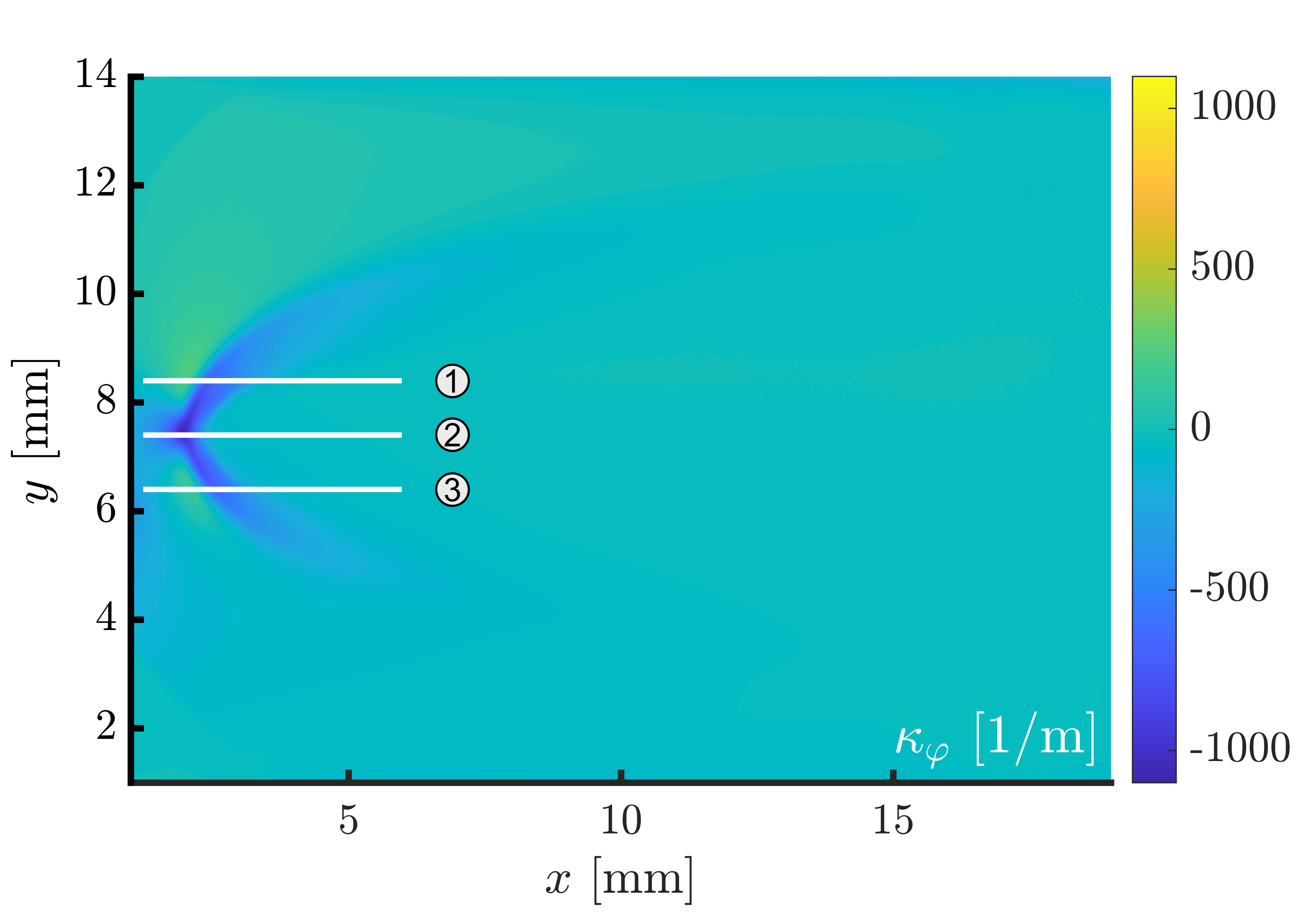
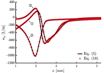
For the verification of Eq. (18), we analyze a methane-air triple flame previously studied in [1]. This flame is established by the consideration of an inflow of premixed fresh gases at atmospheric conditions (300 K and 1 atm) with a mixture stratification in the cross-flow direction. The minimum and maximum mixture fractions at the inlet are 0 and 0.42, respectively, while the imposed mixture fraction gradient is 50 m-1. For more details on this flame, the reader is referred to [1].

Figure 1 displays the $\kappa_{\varphi}$ field associated with the chosen flame (obtained by direct evaluation of Eq. (5)), where three different horizontal slices are identified as representative regions for the aimed validation. In Fig. 2, the corresponding comparison between Eqs. (5) and (18) along the selected slices is shown, where a perfect match is observed. In this way, the validity of the analysis presented in Section 2 is numerically confirmed.

Refer to caption
Figure 2: Profiles of $\kappa_{\varphi}$ along the slices shown in Fig. 1.

4 Two-dimensional flamelet equations with $a_{Z}$ and $a_{\varphi}$ as only parameters

Making use of the obtained relations between the curvatures and the gradients of the conditioning scalars, the two-dimensional flamelet equations derived in [2] for the chemical species mass fractions, $Y_{k}$, and the temperature, $T$, can be rewritten as

$\displaystyle\rho\frac{\partial Y_{k}}{\partial\tau}$ $\displaystyle=-\frac{\partial Y_{k}}{\partial\varphi}\dot{\omega}_{\varphi}+\rho Dg_{Z}^{2}\frac{\partial^{2}Y_{k}}{\partial Z^{2}}+\rho Dg_{\varphi}^{2}\frac{\partial^{2}Y_{k}}{\partial\varphi^{2}}+\dot{\omega}_{k}$ (20)

and

$\displaystyle\rho\frac{\partial T}{\partial\tau}$ $\displaystyle=-\frac{\partial T}{\partial\varphi}\dot{\omega}_{\varphi}+\rho Dg_{Z}^{2}\frac{\partial^{2}T}{\partial Z^{2}}+\rho Dg_{\varphi}^{2}\frac{\partial^{2}T}{\partial\varphi^{2}}+\dot{\omega}_{T}$
$\displaystyle+\frac{\rho D}{c_{p}}\left[g_{Z}^{2}\frac{\partial T}{\partial Z}\frac{\partial c_{p}}{\partial Z}+g_{\varphi}^{2}\frac{\partial T}{\partial\varphi}\frac{\partial c_{p}}{\partial\varphi}\right]$ (21)
$\displaystyle+\sum_{k=1}^{N}\frac{c_{p,k}}{c_{p}}\left[\rho Dg_{Z}^{2}\frac{\partial Y_{k}}{\partial Z}\frac{\partial T}{\partial Z}+\rho Dg_{\varphi}^{2}\frac{\partial Y_{k}}{\partial\varphi}\frac{\partial T}{\partial\varphi}\right],$

respectively. Similarly, the corresponding equations for $g_{Z}$ and $g_{\varphi}$ become

$\displaystyle\frac{\partial g_{Z}}{\partial\tau}$ $\displaystyle=-\left[\frac{g_{\varphi}}{\rho}\frac{\partial}{\partial\varphi}\left(\rho Dg_{\varphi}\right)-D\frac{g_{\varphi}^{2}}{g_{Z}}\frac{\partial g_{Z}}{\partial\varphi}+\frac{\dot{\omega}_{\varphi}}{\rho}\right]\frac{\partial g_{Z}}{\partial\varphi}$
$\displaystyle+\frac{g_{Z}^{2}}{\rho}\frac{\partial^{2}}{\partial Z^{2}}\left(\rho Dg_{Z}\right)-\frac{g_{Z}^{2}}{\rho^{2}}\frac{\partial\rho}{\partial Z}\frac{\partial}{\partial Z}\left(\rho Dg_{Z}\right)$
$\displaystyle-g_{Z}^{2}\frac{\partial}{\partial Z}\left(D\frac{g_{Z}}{g_{\varphi}}\frac{\partial g_{\varphi}}{\partial Z}\right)+g_{Z}a_{Z}$ (22)

and

$\displaystyle\frac{\partial g_{\varphi}}{\partial\tau}$ $\displaystyle=-\left[\frac{g_{Z}}{\rho}\frac{\partial}{\partial Z}\left(\rho Dg_{Z}\right)-D\frac{g_{Z}^{2}}{g_{\varphi}}\frac{\partial g_{\varphi}}{\partial Z}\right]\frac{\partial g_{\varphi}}{\partial Z}$
$\displaystyle+\frac{g_{\varphi}^{2}}{\rho}\frac{\partial^{2}}{\partial\varphi^{2}}\left(\rho Dg_{\varphi}\right)-\frac{g_{\varphi}^{2}}{\rho^{2}}\frac{\partial\rho}{\partial\varphi}\frac{\partial}{\partial\varphi}\left(\rho Dg_{\varphi}\right)$
$\displaystyle-g_{\varphi}^{2}\frac{\partial}{\partial\varphi}\left(D\frac{g_{\varphi}}{g_{Z}}\frac{\partial g_{Z}}{\partial\varphi}\right)+g_{\varphi}^{2}\frac{\partial}{\partial\varphi}\left(\frac{\dot{\omega}_{\varphi}}{\rho g_{\varphi}}\right)+g_{\varphi}a_{\varphi}.$ (23)

As highlighted before, in these equations the only parameters to be imposed are the strain rates $a_{Z}=-\mathbf{n}_{Z}\cdot\nabla\mathbf{u}\cdot\mathbf{n}_{Z}$ and $a_{\varphi}=-\mathbf{n}_{\varphi}\cdot\nabla\mathbf{u}\cdot\mathbf{n}_{\varphi}$, while both curvatures can be now calculated as a flame response.

5 Conclusions

In this work, the recently proposed ($Z,\varphi$) flamelet space has been used to illustrate a so far unnoticed feature common to any orthogonal composition space coordinate system. More specifically, it has been shown how the space orthogonality allows deriving explicit relations between the curvatures, $\kappa_{Z}$ and $\kappa_{\varphi}$, and the gradients of the conditioning scalars, $g_{Z}$ and $g_{\varphi}$. Making use of these relations, both curvatures can be conveniently removed from the corresponding set of two-dimensional orthogonal flamelet equations derived in [2]. With this, the only parameters remaining in the formulation are the two strain rates, $a_{Z}$ and $a_{\varphi}$, solving in this way all problems associated with the closure of curvature in these equations.

Appendix A Mathematical identities

The different components of the curvature tensor, $\nabla\mathbf{n}_{Z}$, can be expressed as

$\displaystyle\frac{\partial n_{i}}{\partial x_{j}}$ $\displaystyle=\frac{\partial}{\partial x_{j}}\left(\frac{1}{g_{Z}}\frac{\partial Z}{\partial x_{i}}\right)$
$\displaystyle=\frac{1}{g_{Z}}\frac{\partial^{2}Z}{\partial x_{i}\partial x_{j}}-\frac{1}{g_{Z}^{2}}\frac{\partial Z}{\partial x_{i}}\frac{\partial g_{Z}}{\partial x_{j}},$ (A.1)

where the second terms at the RHS can be further worked out as

$\displaystyle-\frac{1}{g_{Z}^{2}}\frac{\partial Z}{\partial x_{i}}\frac{\partial g_{Z}}{\partial x_{j}}$ $\displaystyle=-\frac{1}{g_{Z}}n_{i}\frac{\partial}{\partial x_{j}}\left(n_{k}\frac{\partial Z}{\partial x_{k}}\right)$
$\displaystyle=-\frac{1}{g_{Z}}n_{i}n_{k}\left(\frac{\partial^{2}Z}{\partial x_{j}\partial x_{k}}\right)-n_{i}\underbrace{n_{k}\frac{\partial n_{k}}{\partial x_{j}}}_{=0}$ (A.2)

Replacing Eq. (A.2) into (A.1), we obtain

$$\frac{\partial n_{i}}{\partial x_{j}}=\frac{1}{g_{Z}}\left[\frac{\partial^{2}Z}{\partial x_{i}\partial x_{j}}-n_{i}n_{k}\frac{\partial^{2}Z}{\partial x_{j}x_{k}}\right],$$ (A.3)

which corresponds to Eq. (9).

Additionally, the derivatives of $g_{Z}$ in physical space can be rewritten as

$$\frac{\partial g_{Z}}{\partial x_{j}}=\frac{\partial}{\partial x_{j}}\left(n_{i}\frac{\partial Z}{\partial x_{i}}\right),$$ (A.4)

where the RHS can be split as

$$\frac{\partial}{\partial x_{j}}\left(n_{i}\frac{\partial Z}{\partial x_{i}}\right)=n_{i}\frac{\partial^{2}Z}{\partial x_{i}\partial x_{j}}+g_{Z}\underbrace{n_{i}\frac{\partial n_{i}}{\partial x_{j}}}_{=0}.$$ (A.5)

Replacing back in Eq. (A.4), we obtain

$$\frac{\partial g_{Z}}{\partial x_{j}}=n_{i}\frac{\partial^{2}Z}{\partial x_{i}\partial x_{j}},$$ (A.6)

which corresponds to Eq. (14).

Appendix B Alternative derivation of Eq. (18)

In the orthogonal space built by the vectors $\mathbf{n}_{Z}$ and $\mathbf{n}_{\varphi}$, the curvature of the $\varphi$-isosurfaces can be expressed as

$\displaystyle\kappa_{\varphi}$ $\displaystyle=-\nabla\cdot\mathbf{n}_{\varphi}$
$\displaystyle=-\frac{\partial\mathbf{n}_{\varphi}}{\partial n_{Z}}\cdot\mathbf{n}_{Z}-\underbrace{\frac{\partial\mathbf{n}_{\varphi}}{\partial n_{\varphi}}\cdot\mathbf{n}_{\varphi}}_{=0}.$ (B.1)

Making use of the space orthogonality, we obtain the following identity

$$\frac{\partial(\nabla Z\cdot\mathbf{n}_{\varphi})}{\partial n_{Z}}=\nabla Z\cdot\frac{\partial\mathbf{n}_{\varphi}}{\partial n_{Z}}+\mathbf{n}_{\varphi}\cdot\frac{\partial\nabla Z}{\partial n_{Z}}=0,$$ (B.2)

which can be used to obtain Eq. (18) from Eq. (B.1) as

$\displaystyle\kappa_{\varphi}$ $\displaystyle=\frac{1}{g_{Z}}\mathbf{n}_{\varphi}\cdot\frac{\partial\nabla Z}{\partial n_{Z}}$
$\displaystyle=\frac{1}{g_{Z}}\mathbf{n}_{\varphi}\cdot\nabla\left(\frac{\partial Z}{\partial n_{Z}}\right)$
$\displaystyle=\frac{g_{\varphi}}{g_{Z}}\frac{\partial g_{Z}}{\partial\varphi},$ (B.3)

where use has been made of the flamelet transformation $\mathbf{n}_{\varphi}\cdot\nabla(\cdot)=\partial(\cdot)/\partial n_{\varphi}=g_{\varphi}\partial(\cdot)/\partial\varphi$.

References

  • [1] A. Scholtissek, S. Popp, S. Hartl, H. Olguin, P. Domingo, L. Vervisch, C. Hasse, Derivation and analysis of two-dimensional composition space equations for multi-regime combustion using orthogonal coordinates, Combust. Flame 218 (2020) 205 – 217.
  • [2] H. Olguin, P. Domingo, L. Vervisch, C. Hasse, A. Scholtissek, A self-consistent extension of flamelet theory for partially premixed combustion, Combustion and Flame 255 (2023) 112911.
  • [3] M. Matalon, On flame stretch, Combustion Science and Technology 31 (1983) 169–181.
  • [4] S. Chung, C. Law, An invariant derivation of flame stretch, Combustion and Flame 55 (1984) 123–125.
  • [5] L. P. H. de Goey, J. H. M. ten Thije Boonkkamp, A mass-based definition of flame stretch for flames with finite thickness, Combust. Sci. Technol. 122 (1997) 399–405.
  • [6] C. Kortschik, S. Honnet, N. Peters, Influence of curvature on the onset of autoignition in a corrugated counterflow mixing field, Combust. Flame 142 (2005) 140 – 152.
  • [7] H. Xu, F. Hunger, M. Vascellari, C. Hasse, A consistent flamelet formulation for a reacting char particle considering curvature effects, Combust. Flame 160 (2013) 2540 – 2558.
  • [8] Y. Xuan, G. Blanquart, M. E. Mueller, Modeling curvature effects in diffusion flames using a laminar flamelet model, Combust. Flame 161 (2014) 1294 – 1309.
  • [9] A. Scholtissek, W. L. Chan, H. Xu, F. Hunger, H. Kolla, J. H. Chen, M. Ihme, C. Hasse, A multi-scale asymptotic scaling and regime analysis of flamelet equations including tangential diffusion effects for laminar and turbulent flames, Combust. Flame 162 (2015) 1507 – 1529.
  • [10] C. Dopazo, J. Martín, Local geometry of isoscalar surfaces, Phys. Rev. E 76 (2007) 056326.
  • [11] F. A. Williams, Combustion Theory, 2nd Edition, The Benjamin/Cummings Publishing Company, Inc, 1985.