Factor Augmented Tensor-on-Tensor Neural Networks

Abstract

This paper studies the prediction task of tensor-on-tensor regression in which both covariates and responses are multi-dimensional arrays (a.k.a., tensors) across time with arbitrary tensor order and data dimension. Existing methods either focused on linear models without accounting for possibly nonlinear relationships between covariates and responses, or directly employed black-box deep learning algorithms that failed to utilize the inherent tensor structure. In this work, we propose a Factor Augmented Tensor-on-Tensor Neural Network (FATTNN) that integrates tensor factor models into deep neural networks. We begin with summarizing and extracting useful predictive information (represented by the “factor tensor”) from the complex structured tensor covariates, and then proceed with the prediction task using the estimated factor tensor as input of a temporal convolutional neural network. The proposed methods effectively handle nonlinearity between complex data structures, and improve over traditional statistical models and conventional deep learning approaches in both prediction accuracy and computational cost. By leveraging tensor factor models, our proposed methods exploit the underlying latent factor structure to enhance the prediction, and in the meantime, drastically reduce the data dimensionality that speeds up the computation. The empirical performances of our proposed methods are demonstrated via simulation studies and real-world applications to three public datasets. Numerical results show that our proposed algorithms achieve substantial increases in prediction accuracy and significant reductions in computational time compared to benchmark methods.

Keywords: Tensor regression; Tensor-on-tensor regression; Tensor factor model;
Time series forecasting; Temporal convolutional network.

1 Introduction

Motivated by a wide range of industrial and scientific applications, forecasting tasks using one tensor series to predict another has become increasingly prevalent in various fields. In finance, tensor models are used to forecast future stock prices by analyzing multi-dimensional stock attributes over time (Tran et al.,, 2017). In meteorology, tensor models predict future weather conditions using historical data formatted as multi-dimensional tensors (latitude, longitude, time, etc.) (Bilgin et al.,, 2021). In neuroscience, tensor models are employed to process medical imaging like MRI/fMRI scans (Wei et al.,, 2023).

Though predictive modeling of tensors has emerged rapidly over the past decade, most existing studies primarily focus on scenarios when either covariates or responses are tensors, such as scalar-on-tensor regression (Guo et al.,, 2011; Zhou et al.,, 2013; Wimalawarne et al.,, 2016; Li et al.,, 2018; Ahmed et al.,, 2020), matrix-on-tensor regression (Hoff,, 2015; Kossaifi et al.,, 2020), and tensor response regression (Li and Zhang,, 2017; Sun and Li,, 2017). Tensor-on-tensor prediction, when both covariates and responses are tensors, remains a challenging task due to the inherent complexities of tensor structures.

One commonly used strategy for tensor-on-tensor modeling is to flatten the tensors into matrics (or even vectors) (Kilmer and Martin,, 2011; Choi and Vishwanathan,, 2014) so that matrix-based analytical tools become applicable. However, flattening can lead to a loss of spatial or temporal information, especially for datasets that are inherently dependent on data structures. For instance, in image processing, the relative positions of pixels carry important information about object shapes, which is lost when the image is flattened.

Alternatively, there is a handful of recent works on tensor-on-tensor regression models that do not adopt flattening but deal with the tensor structures directly; see Lock, (2018); Liu et al., (2020); Gahrooei et al., (2021); Luo and Zhang, (2022). However, these methods posit a linear prediction model between covariates and responses, limiting their capacity to capture potential nonlinear relationships.

Another emerging trend in tensor-on-tensor prediction involves neural networks, such as recurrent neural networks, convolutional neural networks, convolutional recurrent neural networks, and temporal convolutional networks, to name a few. Deep neural network is a powerful tool in prediction tasks owing to its ability to learn intricate patterns from complex datasets. Structured with multiple layers of interconnected neurons, neural networks excel in capturing nonlinearity in data. Nevertheless, they often operate in a black-box manner and typically require extensive computational resources.

In this work, we develop a Factor Augmented Tensor-on-Tensor Neural Network (FATTNN) for forecasting a sequence of tensor responses using tensor covariates of arbitrary tensor order and data dimensions. One key innovation of our method is the integration of tensor factor models into deep neural networks for tensor-on-tensor regression. Factor models have been a widely utilized tool in matrix/vector data analysis (Bai and Ng,, 2002; Stock and Watson,, 2002; Pan and Yao,, 2008; Lam and Yao,, 2012) for understanding common dependence among multi-dimensional covariates. In recent years, researchers have advanced the methodology of factor models to the context of tensor time series (Chen et al., 2022a, ; Chen et al., 2022b, ; Han et al.,, 2020, 2024, 2022; Han and Zhang,, 2022). In our models, we borrow the strengths from tensor factor models, offering a more general approach than traditional vector factor analysis for prediction (Sen et al.,, 2019; Fan et al.,, 2017; Yu et al.,, 2022).

Our contributions can be summarized in three folds.

• We propose a FATTNN model for tensor-on-tensor prediction that integrates tensor factor models into deep neural networks. Via a tensor factor model, FATTNN exploits the latent factor structures among the complex structured tensor covariates, and extracts useful predictive information for subsequent modeling. The utilization of the factor model reduces the data dimension drastically while preserving the tensorial data structures, contributing to substantial increases in prediction accuracy and significant reductions in computational time.

• In addition to the improved prediction accuracy and reduced computation cost, FATTNN offers several advantages over existing methods. First, it preserves the inherent tensor structure without any flattening or tensor contraction operations, preventing the possible loss of spatial or temporal information. Second, the utilization of neural networks equips FATTNN with exceptional capability in modeling nonlinearity in response-covariate relationships.

• FATTNN provides a comprehensive framework for the general supervised learning question of predicting tensor responses using tensor covariates. Although initially introduced under the problem settings of tensor-on-tensor time series forecasting, the proposed FATTNN framework is not limited to time series data, but can accommodate a variety of data types. With different types of factor models and choices of neural network architectures tailored to specific characteristics of the data, FATTNN can be naturally adapted to tensor-on-tensor regression for various data types.

This paper is organized as follows. Section 2 introduces some useful tensor terminology and sets up the problem of interest. Section 3 presents the methodological details of the proposed FATTNN algorithms. Section 4 includes applications to three real-world datasets to demonstrate the finite-sample performance of our proposed methods. Section 5 concludes the paper with discussions. Theoretical proofs, simulation studies, and supplemental numerical results are provided in appendices.

2 Preliminaries

Notation. Before proceeding, we first set up some notation. Let $\mathcal{X}\in\mathbb{R}^{d_{1}\times\dots\times d_{K}}$ denote a $K$-th order tensor of dimension $d_{1}\times d_{2}\times\dots\times d_{K}$. Let $\mathcal{X}_{i_{1},\dots,i_{K}}$ denote the $({i_{1},\dots,i_{K}})$-th entry of the tensor $\mathcal{X}$ and $\mathcal{X}[\mathcal{I}_{1},\dots,\mathcal{I}_{K}]$ denotes the sub-tensor of $\mathcal{X}$ for $\mathcal{I}_{1}\subseteq\{1,\dots,d_{1}\},\dots,\mathcal{I}_{K}\subseteq\{1,\dots,d_{K}\}$. The matricization operation $\hbox{\rm mat}_{k}(\cdot)$ unfolds an order-$K$ tensor along mode $k$ to a matrix, say ${\cal X}\in\mathbb{R}^{d_{1}\times\dots\times d_{K}}$ to $\hbox{\rm mat}_{k}({\cal X})\in\mathbb{R}^{d_{k}\times d_{-k}}$ where $d_{k}=\prod_{j\neq k}d_{j}$ and its detailed definition is provided in the appendix. The Frobenius norm of tensor ${\cal X}$ is defined as $\|{\cal X}\|_{\rm F}=(\sum_{i_{1},i_{2},\cdots,i_{K}}{\cal X}_{i_{1},\dots,i_{K}}^{2})^{1/2}$. The Tucker rank of an order-$K$ tensor ${\cal X}$, denoted by Tucrank$({\cal X})$, is defined as a $K$-tuple $(r_{1},...,r_{K})$, where $r_{k}=\text{rank}(\hbox{\rm mat}_{k}({\cal X}))$. Any Tucker rank-$(r_{1},...,r_{K})$ tensor ${\cal X}$ admits the following Tucker decomposition (Tucker,, 1966): ${\cal X}={\cal S}\times_{1}U_{1}\times_{2}\cdots\times_{K}U_{K}$, where ${\cal S}\in\mathbb{R}^{r_{1}\times\cdots\times r_{K}}$ is the core tensor and $U_{k}=\text{SVD}_{r_{k}}(\hbox{\rm mat}_{k}({\cal X}))$ is the mode-$k$ top $r_{k}$ left singular vectors. Here, the mode-$k$ product of ${\cal X}\in\mathbb{R}^{d_{1}\times\cdots\times d_{K}}$ with a matrix $B\in\mathbb{R}^{d_{k}\times r_{k}}$, denoted by ${\cal X}\times_{k}B$, is a $d_{1}\times\cdots\times d_{k-1}\times r_{k}\times d_{k+1}\times\cdots\times d_{K}$-dimensional tensor, and its detailed definition is provided in Section 3 and Appendix A. The following abbreviations are used to denote the tensor-matrix product along multiple modes: ${\cal X}\times_{k=1}^{K}U_{k}={\cal X}\times_{1}U_{1}\times_{2}\cdots\times_{K}U_{K}$ and ${\cal X}\times_{\ell\neq k}U_{\ell}={\cal X}\times_{1}U_{1}\times_{2}\cdots\times_{k-1}U_{k-1}\times_{k+1}U_{k+1}\times_{k+2}\cdots\times_{K}U_{K}$. For any two matrices $A\in\mathbb{R}^{m_{1}\times r_{1}},B\in\mathbb{R}^{m_{2}\times r_{2}}$, denote the Kronecker product $\odot$ as $A\odot B\in\mathbb{R}^{m_{1}m_{2}\times r_{1}r_{2}}$. For any two tensors ${\cal A}\in\mathbb{R}^{m_{1}\times m_{2}\times\cdots\times m_{K}},{\cal B}\in\mathbb{R}^{r_{1}\times r_{2}\times\cdots\times r_{N}}$, denote the tensor product $\otimes$ as ${\cal A}\otimes{\cal B}\in\mathbb{R}^{m_{1}\times\cdots\times m_{K}\times r_{1}\times\cdots\times r_{N}}$, such that $({\cal A}\otimes{\cal B})_{i_{1},...,i_{K},j_{1},...,j_{N}}=({\cal A})_{i_{1},...,i_{K}}({\cal B})_{j_{1},...,j_{N}}.$

Problem Setup. Suppose we observe a time series dataset comprising $n$ temporal samples ${\cal D}=\{({\cal X}_{t},{\cal Y}_{t}),1\leq t\leq n\}$, where $\mathcal{X}_{t}\in\mathbb{R}^{d_{1}\times\dots\times d_{K}}$ is a tensor of covariates and $\mathcal{Y}_{t}\in\mathbb{R}^{p_{1}\times\dots\times p_{q}}$ is the tensor response variable. For some newly observed covariates $\{{\cal X}_{t}\}_{t=n+1}^{n+m}$, the forecasting task of tensor-on-tensor time series regression is to accurately predict the corresponding future tensor responses $\{{\cal Y}_{t}\}_{t=n+1}^{n+m}$, given the observed time series $\{({\cal X}_{t},{\cal Y}_{t})\}_{t=1}^{n}$ and the new covariates $\{{\cal X}_{t}\}_{t=n+1}^{n+m}$. Here, $m$ is the forecast horizon. In subsequent discussions, we denote the series in training time range as $\mathcal{X}^{(tr)}=\{\mathcal{X}_{t}\}_{t=1}^{n}$ and $\mathcal{Y}^{(tr)}=\{\mathcal{Y}_{t}\}_{t=1}^{n}$, and the covariates in forecasting time range as $\mathcal{X}^{(te)}=\{\mathcal{X}_{t}\}_{t=n+1}^{n+m}$.

3 Methodology: Factor Augmented Tensor-on-Tensor time series regression

In this section, we introduce our Factor Augmented Tensor-on-Tensor Neural Network, dubbed as FATTNN. Our work explores a broad category of challenges known as tensor-on-tensor regression, which seeks to elucidate the relationships between covariates and responses that may manifest as scalars, vectors, matrices, or higher-order tensors. As illustrated in Figure 1, our method consists of two components. First, factor tensor features are extracted by low-rank tensor factorization. Second, we develop a Tensor-on-Tensor Neural Network based on Temporal Convolutional Network (TCN) (Bai et al.,, 2018). In Section 3.1, we present a tensor factor model. This model can capture global patterns among the observed time series covariate tensors, by representing each of the original covariate tensor ${\cal X}_{t}$ as a multilinear combination of $r_{1}\times\cdots\times r_{K}$ basis across each tensor mode $k$ plus noise, where $r_{k}\ll d_{k}$. It offers a more general approach than the traditional vector factor analysis for prediction (Sen et al.,, 2019; Fan et al.,, 2017; Luo et al.,, 2022; Yu et al.,, 2022; Fan and Gu,, 2023), and preserves the tensor structures of features. It also provides dimension reduction, which significantly reduces computational complexity. In Section 3.2, we describe how the output from the global tensor factor model can be used as an input covariate for a TCN to predict future response tensors.

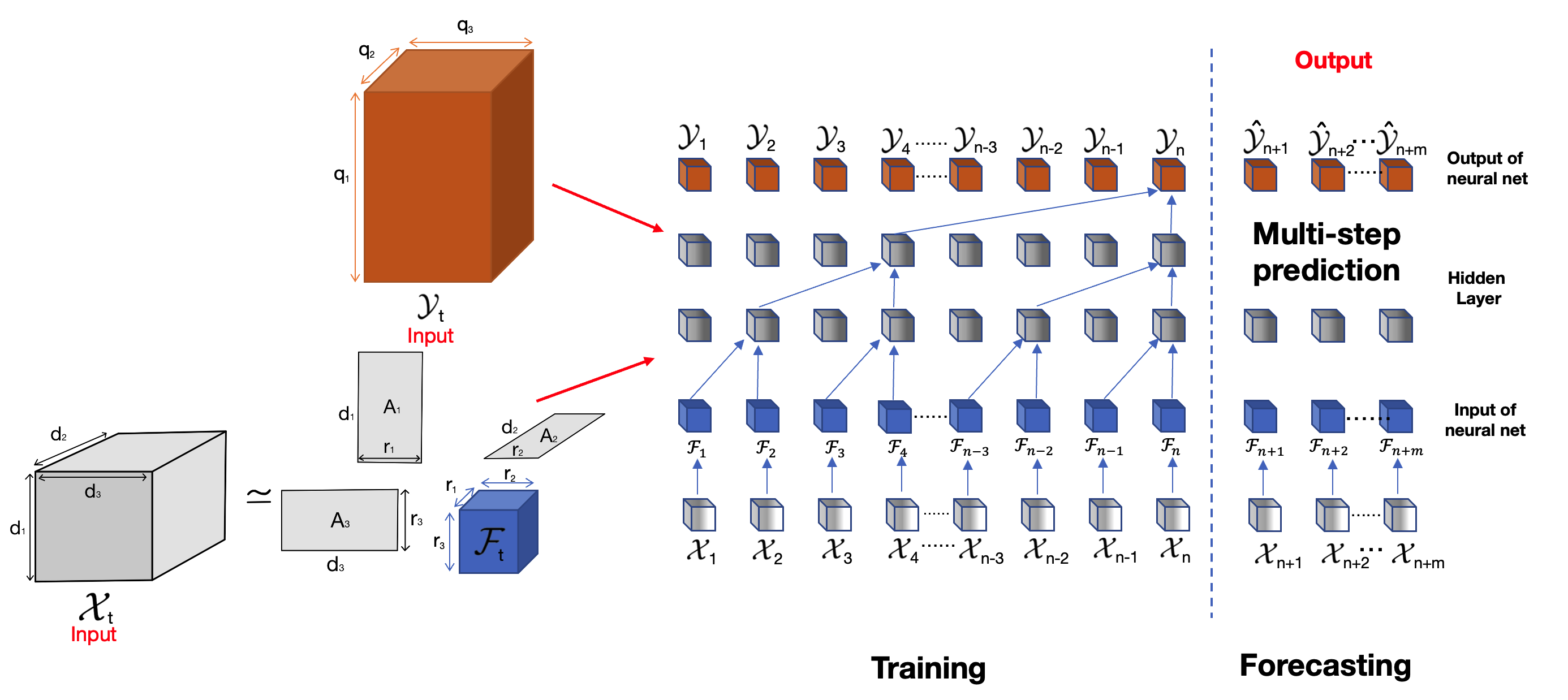
Figure 1: A graphical illustration of the proposed FATTNN.
The input is the observed time series $\{({\cal X}_{t},{\cal Y}_{t})\}_{t=1}^{n}$ and the new covariates $\{{\cal X}_{t}\}_{t=n+1}^{n+m}$.
The output is the forecasted future tensor responses, denoted by $\{\widehat{\cal Y}_{t}\}_{t=n+1}^{n+m}$

3.1 Tensor Factor Model (TFM)

Our representation learning module utilizes low rank tensor factorization for covariate tensor. The idea is to factorize the training covariate tensors ${\cal X}_{t}\in\mathbb{R}^{d_{1}\times\cdots\times d_{K}},1\leq t\leq n,$ into low dimensional tensors ${\cal F}_{t}\in\mathbb{R}^{r_{1}\times\cdots\times r_{K}}$ and linear combination matrices (loading matrices) $A_{k}\in\mathbb{R}^{d_{k}\times r_{k}}$, where $r_{k}\ll d_{k}$. Specifically, the model can be expressed as

$$\mathcal{X}_{t}=\mathcal{F}_{t}\times_{1}A_{1}\times_{2}\ldots\times_{K}A_{K}+{\cal E}_{t},$$ (1)

where ${\cal E}_{t}$ is idiosyncratic noise of the tensor ${\cal X}_{t}$, and $t$ is a time point. Here the $k$-mode product of $\mathcal{X}\in\mathbb{R}^{d_{1}\times d_{2}\times\ldots\times d_{K}}$ with a matrix $U\in\mathbb{R}^{d_{k}^{\prime}\times d_{k}}$, denoted as $\mathcal{X}\times_{k}U$, is an order $K$-tensor of size $d_{1}\times\ldots\times d_{k-1}\times d_{k}^{\prime}\times d_{k+1}\times\ldots\times d_{K}$ such that $(\mathcal{X}\times_{k}U)_{i_{1},\ldots,i_{k-1},j,i_{k+1},\ldots,i_{K}}=\sum_{i_{k}=1}^{d_{k}}\mathcal{X}_{i_{1},i_{2},\ldots,i_{K}}U_{j,i_{k}}.$ If $K=2$, the matrix factor model can be written as ${\cal X}_{t}=A_{1}{\cal F}_{t}A_{2}^{\top}+{\cal E}_{t}$. The latent core tensor ${\cal F}_{t}$, which typically encapsulates the most critical information, generally possesses dimensions significantly smaller than those of ${\cal X}_{t}$. Thus, the covariate tensor ${\cal X}_{t}$ can be thought of to be comprised of a basis tensor features ${\cal F}_{t}$ that capture the global patterns in the whole data-set, and all the original covariates are multilinear combinations of these basis tensor features. In the following subsection, we will discuss how a TCN can be utilized to leverage the temporal structure of the training data.

For predicting future response tensors, given a new covariate tensor ${\cal X}_{t}$, we can also extract low-dimensional feature tensors ${\cal F}_{t}$ using the estimated deterministic loading matrices $A_{k}$ and model (1). This approach efficiently captures the essential characteristics from the high-dimensional input data. The reduced dimensionality allows for more efficient data processing and analysis while retaining essential features.

To capture the underlying tensor features of the covariates, we employ a Time series Inner-Product Unfolding Procedure (TIPUP). It utilizes the linear temporal dependence among the covariates. The TIPUP method performs singular value decomposition (SVD) for each tensor mode $k=1,...,K$:

$$\widehat{A}_{k}=\text{LSVD}_{r_{k}}\left(\frac{1}{n}\sum_{t=1}^{n}\hbox{\rm mat}_{k}({\cal X}_{t})\hbox{\rm mat}_{k}^{\top}({\cal X}_{t})\right).$$ (2)

The estimation methods in (2) can be further enhanced through an iterative refinement algorithm, detailed in the appendix. The factor tensors in the training data thus can be estimated by

$$\widehat{\cal F}_{t}={\cal X}_{t}\times_{k=1}^{K}\widehat{A}_{k}^{\top},\quad\text{for }1\leq t\leq n.$$

In the next proposition, we demonstrate the provable benefits of using a tensor factor model with Tucker low-rank structure (1). Specifically, we establish the convergence rates of the linear space of the loading matrices, which in turn ensure the accuracy of the estimated factor tensors.

Proposition 3.1.

Assume each elements of the idiosyncratic noise ${\cal E}_{t}$ in (1) are i.i.d. $N(0,1)$. The ranks $r_{1},...,r_{K}$ are fixed. The factor process ${\cal F}_{t}$ is weakly stationary and its cross-outer-product process is ergodic in the sense of $\frac{1}{n}\sum_{t=1}^{n}{\cal F}_{t}\otimes{\cal F}_{t}\rightarrow\mathbb{E}({\cal F}_{t}\otimes{\cal F}_{t})$ in probability, where the elements of $\mathbb{E}({\cal F}_{t}\otimes{\cal F}_{t})$ are all finite. In addition, the condition numbers of $A_{k}^{\top}A_{k}$ ($k=1,...,K$) are bounded. Let $\lambda=\prod_{k=1}^{K}\|A_{k}\|_{2}$ and grow as dimensions $d_{k}$ increases. Then, the iterative TIPUP estimator satisfies

$$\|\widehat{A}_{k}(\widehat{A}_{k}^{\top}\widehat{A}_{k})^{-1}\widehat{A}_{k}^{\top}-A_{k}(A_{k}^{\top}A_{k})^{-1}A_{k}\|_{2}=O_{\mathbb{P}}\left(\frac{\max_{k}\sqrt{d_{k}}}{\lambda\sqrt{n}}+\frac{\max_{k}\sqrt{d_{k}}}{\lambda^{2}\sqrt{n}}\right),\qquad 1\leq k\leq K.$$

3.2 Tensor-on-Tensor Neural Network based TCN (TTNN)

If we are equipped with a TCN that identifies the temporal patterns in the training dataset $({\cal X}^{(tr)},{\cal Y}^{(tr)})$, we can use this model to enhance the temporal structures in $({\cal F}^{(tr)},{\cal Y}^{(tr)})$. Thus, a TCN is applied to the input sequence of estimated factor tensors $\widehat{\cal F}_{1},\ldots,\widehat{\cal F}_{t}$ along with the corresponding output sequence of response tensors ${\cal Y}_{1},\ldots,{\cal Y}_{t}$ to encapsulate the temporal dynamics. Let $\eta(\cdot)$ represent this network. The whole temporal network $\eta(\cdot)$ can be trained using the low-rank factor tensors $\widehat{\cal F}_{1},\ldots,\widehat{\cal F}_{n}$ derived from the training dataset.

The trained temporal network $\eta(\cdot)$ can be effectively utilized for multi-step look-ahead prediction in a standard approach. The factor tensors for future time steps can be estimated using the following formula:

$$\widehat{\cal F}_{n+h}={\cal X}_{n+h}\times_{k=1}^{K}\widehat{A}_{k}^{\top},$$

where $h>0$. Using the historical data points of factor tensors $\widehat{\cal F}_{t},1\leq t\leq n+h-1$, the prediction for the subsequent time step, ${\cal Y}_{n+h}$, is generated by

$$\widehat{\cal Y}_{n+h}=\eta(\widehat{\cal F}_{1},...,\widehat{\cal F}_{n+h}).$$

Our hybrid forecasting model incorporates a TCN that inputs past data points from the original raw response time series and the estimated factor tensors, enhancing prediction accuracy. The pseudo-code for our model is outlined in Algorithm 1.

Algorithm 1 Factor Augmented Tensor-on-Tensor Neural Network (FATTNN)

1:  Input: Observed tensor time series $(\mathcal{X}_{1},\mathcal{Y}_{1}),\ldots,(\mathcal{X}_{n},\mathcal{Y}_{n}),\mathcal{X}_{n+1},\ldots,\mathcal{X}_{n+m}$, rank $r_{k}$ for each mode $k$, forecasting horizon $m$.

2:  Output: Forecasts $\widehat{\mathcal{Y}}_{n+1},\ldots,\widehat{\mathcal{Y}}_{n+m}$.

3:  Compute the factor tensor $\widehat{\cal F}_{t}$ for $t=1,\ldots,n$ by TIPUP (2) or its iterative version in Algorithm S.1.

4:  Fit a TCN $\eta(\cdot)$ to the input sequence of factor tensors $\widehat{\cal F}_{1},\ldots,\widehat{\cal F}_{n}$ and the output sequence of response tensor ${\cal Y}_{1},...,{\cal Y}_{n}$ to capture the temporal dynamics.

5:  Forecast ${\cal Y}_{n+1},\ldots,{\cal Y}_{n+m}$ using the fitted TCN.

6:  for $h=1$ to $m$ do

7:     $\widehat{\cal F}_{n+h}={\cal X}_{n+h}\times_{k=1}^{K}\widehat{A}_{k}^{\top}$.

8:     $\widehat{\mathcal{Y}}_{n+h}=\eta(\widehat{\cal F}_{1},\ldots,\widehat{\mathcal{F}}_{n+h})$.

9:  end for

10:  return  $\widehat{\mathcal{Y}}_{n+1},\ldots,\widehat{\mathcal{Y}}_{n+m}$.

4 Numerical Results

In this section, we investigate the finite-sample performance of our proposed FATTNN methods via simulation studies and real-world applications. Specifically, we implement the proposed FATTNN with TIPUP algorithm to estimate the factor structures. For benchmark methods , we consider one traditional statistical model - the multiway tensor-on-tensor regression (Lock,, 2018) (denoted by Multiway), and one conventional deep learning approach – the temporal convolutional network (Bai et al.,, 2018) of $\mathcal{Y}$ regressed on $\mathcal{X}$ (denoted by TCN). Due to space limitations, simulation results are presented in Appendix 4.1.

Evaluation Metrics. We evaluate the performance of various methods with emphasis on two aspects: prediction accuracy and computational efficiency. To evaluate prediction accuracy, we compute the Mean Squared Error (MSE) over the testing data, i.e., $\text{MSE}=(n_{\text{test}}\cdot p_{1}\cdots p_{q})^{-1}\sum_{i\in\mathcal{D}_{\text{test}}}\|\mathcal{Y}_{i}^{(\text{obs})}-\mathcal{Y}_{i}^{(\text{pred})}\|_{F}^{2}$, where $\mathcal{D}_{\text{test}}$ denotes the testing set, $n_{\text{test}}$ is the number of samples in the testing set $\mathcal{D}_{\text{test}}$, and $(\mathcal{Y}_{i}^{(\text{obs})},\mathcal{Y}_{i}^{(\text{pred})})$ are the observed and predicted values of the $i$-th tensor response. In addition, we record the computational time of different methods to evaluate computational efficiency.

4.1 Simulation Studies

We carry out simulation studies under different scenarios with various configurations of sample size, data dimensions, tensor ranks, and relationships between covariates and responses. Recall that ${\cal X}_{t}\in\mathbb{R}^{d_{1}\times\cdots\times d_{K}}$, ${\cal F}_{t}\in\mathbb{R}^{r_{1}\times\cdots\times r_{K}}$, ${\cal Y}_{t}\in\mathbb{R}^{p_{1}\times\cdots\times p_{q}}$, for $1\leq t\leq n$.

Data Generating Process. We begin with generating the low-rank core tensor ${\cal F}_{t}$ from a tensor autoregressive model ${\rm vec}({\cal F}_{t})=\Phi\cdot{\rm vec}({\cal F}_{t-1})+{\rm vec}({\cal W}_{t})$ for $t=1,\ldots,n$. Here, ${\rm vec}({\cal F}_{t})$ denotes the vectorization of a tensor ${\cal F}_{t}$, ${\cal W}_{t}\in\mathbb{R}^{r_{1}\times\cdots\times r_{K}}$ is an error tensor in which every element is randomly generated from a normal distribution. The coefficient matrix $\Phi\in\mathbb{R}^{(r_{1}r_{2}\cdots r_{K})\times(r_{1}r_{2}\cdots r_{K})}$ is constructed using the Kronecker product of a sequence of matrices $Q_{k}$, i.e., $\Phi=\odot_{k=1}^{K}Q_{k}$, in which each $Q_{k}\in\mathbb{R}^{r_{k}\times r_{k}}$ is a matrix with i.i.d. standard normal entries and orthonormalized through QR decomposition. The tensor time series ${\cal F}_{t}$ is randomly initiated in a distance past, and we discard the first 500 time points to stabilize the process.

Next, we generate the tensor covariates ${\cal X}_{t}$ from ${\cal F}_{t}$, following $\mathcal{X}_{t}=\lambda\mathcal{F}_{t}\times_{1}A_{1}\times_{2}\ldots\times_{K}A_{K}+{\cal E}_{t},$ for $t=1,\ldots n$, where $\lambda$ is a scalar that controls the signal-to-noise ratio in the tensor factor model. In our experiments, we set $\lambda=(\prod_{k=1}^{K}r_{k})^{1/2}$. The loading matrices $A_{k}\in\mathbb{R}^{d_{k}\times r_{k}}$ are generated with independent $N(0,1)$ entries, and then orthonormalized using QR decomposition. The error ${\cal E}_{t}\in\mathbb{R}^{d_{1}\times\cdots\times d_{K}}$ is also generated with each element independently drawn from normal distributions.

Then, we generate the tensor responses ${\cal Y}_{t}$ from ${\cal F}_{t}$, using ${\cal Y}_{t}=\langle S({\cal F}_{t}),\Lambda\rangle_{L}+{\cal U}_{t}$, $t=1,\ldots n$. Here $S({\cal F}_{t}):=(s({\cal F}_{t,i_{1},\ldots,i_{K}}))_{1\leq i_{1}\leq r_{1},\ldots,1\leq i_{K}\leq r_{K}}\in\mathbb{R}^{r_{1}\times\cdots\times r_{K}}$ applies an element-wise transformation $s(\cdot)$ to each entry of ${\cal F}_{t}$. ${\cal U}_{t}\in\mathbb{R}^{p_{1}\times\cdots\times p_{q}}$ is a noise matrix whose elements are i.i.d $N(0,\sigma_{u}^{2})$. The coefficient tensor $\Lambda$ is set as $\Lambda=\llbracket U_{1},\cdots,U_{K},V_{1},\cdots V_{d}\rrbracket\in\mathbb{R}^{r_{1}\times\cdots\times r_{K}\times p_{1}\times\cdots\times p_{q}}$ where $U_{k}\in\mathbb{R}^{r_{k}\times R}$ for $k=1,\cdots,K$ and $V_{m}\in\mathbb{R}^{p_{m}\times R}$ for $m=1,\cdots,d$, each with independent $N(0,1)$ entries. In our experiments, we set $R=6$. Details of the notation $\llbracket\ \cdot,\cdots,\cdot\ \rrbracket$ and $\langle\cdot,\cdot\rangle_{L}$ are provided in Equations (S.21) and (S.22) of Appendix B.

We consider the following three experimental configurations:

1. $(d_{1},d_{2},d_{3})=(25,25,12)$,$(r_{1},r_{2},r_{3})=(6,8,6)$, $(p_{1},p_{2},p_{3})=(3,3,2)$
   $n=500$, $s(z)=cos(z)$, $\sigma_{u}^{2}=1$.

2. $(d_{1},d_{2},d_{3})=(30,6,12)$, $(r_{1},r_{2},r_{3})=(6,3,2)$, $(p_{1},p_{2},p_{3})=(8,6,4)$,
   $n=400$, $s(z)=log(|z|)$, $\sigma_{u}^{2}=1$.

3. $(d_{1},d_{2},d_{3})=(12,3,12)$, $(r_{1},r_{2},r_{3})=(4,3,4)$, $(p_{1},p_{2},p_{3})=(3,3,3)$,
   $n=100$, $s(z)=log(e^{(z)}+1)$, $\sigma_{u}^{2}=0.5$.

Simulation Evaluations. In each setting, we use 70% for training the models and 30% for model evaluation. Comparisons of MSE, and computational time are summarized in Table 1 and Table 2. All reported metrics are averaged over 20 replications. Experiments were run on the research computing cluster provided by the University Center for Research Computing. From Table 1, we can see that FATTNN improves over the two benchmark methods by a large margin. The improvements can be attributed to two facets: (a) the utilization of tensor factors, summarizing useful predictive information effectively and reducing the number of noise covariates, and (b) the utilization of neural networks, possessing extraordinary ability in capturing complex relationships in the data and therefore exhibiting exceptional predictive power. On a separate note, Table 2 reveals the evident computational advantage of FATTNN compared to other neural network models such as TCN, owing to the effective dimension reduction through tensor factor models.

Table 1: Comparisons of prediction accuracy of different methods in simulation studies
(measured by MSE over the testing data)

Prediction Task	TCN	FATTNN	MultiWay
Simulation 1	3.642 (1.91)	2.451 (1.57)	3.987 (2.00)
Simulation 2	670.5 (25.8)	511.9 (22.5)	805.1 (28.4)
Simulation 3	1074 (32.6)	696.7 (26.4)	1670 (40.3)

Note: The results are averaged over 20 replications.
Numbers in the brackets are standard errors.

Table 2: Comparisons of computational time (in the format of hh:mm:ss)
of different methods in simulation studies

Prediction Task	TCN	FATTNN	Muiltway
Simulation 1	01:22:02	00:16:18	00:02:15
Simulation 2	01:26:30	00:17:54	00:02:30
Simulation 3	00:11:16	00:03:41	00:01:03

4.2 Real Data Examples

We evaluate the performance of different methods using five prediction tasks on three real-world datasets. The information about sample sizes in the datasets, data dimensions of covariates $(d_{1},\ldots,d_{K})$ and responses $(p_{1},\ldots,p_{q})$, and the ranks of core tensors $(r_{1},\ldots,r_{K})$ utilized in the analyses are summarized in Table 3. For the prediction tasks using the New York Taxi data and FMRI image datasets, we split the data into training sets (70%) and testing (30%). For the prediction tasks using the FAO dataset, we use 80% data for training and 20% for testing due to its relatively small sample size. We compare the prediction accuracy and computation time of three methods: FATTNN, TCN, and Multiway. The numerical prediction results along with the corresponding computation time are summarized in Table 4.

Table 3: Data information of the real-world applications

Prediction Task	Sample Size	Dimension of $\mathcal{X}_{t}$	Dimension of $\mathcal{Y}_{t}$	Rank of ${\cal F}_{t}$
FAO crop $\sim$ crop	62	(33,2,11)	(13,2,11)	(6,2,4)
FAO crop $\sim$ livestock	62	(26,4,5)	(26,3,11)	(6,4,2)
NYC taxi – midtown	504	(2,12,12,8)	(2,12,12,8)	(2,4,4,2)
NYC taxi – downtown	504	(2,19,19,8)	(2,19,19,8)	(2,4,4,2)
FMRI data	1452	(25,64,64)	(1,64,64)	(8,23,23)

Table 4: Comparisons of prediction accuracy (measured by MSE over the testing data) and computational time (in the format of hh:mm:ss) of different methods in real-world applications

	MSE			Time
Prediction Task	TCN	FATTNN	Multiway	TCN	FATTNN	Multiway
FAO crop $\sim$ crop	14.11	7.437	12.29	00:55:33	00:15:28	00:03:18
FAO crop$\sim$ livestock	32.53	21.65	48.04	00:24:34	00:12:57	00:03:21
NYC taxi – midtown	12.87	7.399	22.84	01:57:15	00:34:34	00:04:52
NYC taxi – downtown	14.58	9.493	28.10	03:25:55	00:32:46	00:25:35
FMRI data	0.1236	0.06634	0.1397	03:54:50	00:20:58	10:01:20

(1) The United Nations Food and Agriculture Organization (FAO) Crops and Livestock Products Data. The database provides agricultural statistics (including crop, livestock, and forestry sub-sectors) collected from countries and territories since 1961. It is publicly available at https://www.fao.org/faostat/en/#data/QCL. Our analyses focus on 11 crops and 5 livestock products of 46 countries in East Asia, North America, South America, and Europe from 1961 to 2022. Detailed information about the types of crops, livestock, and countries are presented in Table S.1 of Appendix B. We study two prediction tasks using the FAO dataset: (i) using Yield and Production data of 11 different crops for 33 countries in East Asia, North America, and Europe (i.e., ${\cal X}_{t}\in\mathbb{R}^{33\times 2\times 11}$) to predict the Yield and Production quantities of the same crops for 13 selected countries in South America (i.e., ${\cal Y}_{t}\in\mathbb{R}^{13\times 2\times 11}$); and (ii) using four agricultural statistics (Producing Animals, Animals-slaughtered, Milk Animals, Laying) associated with 5 kinds of livestock of 26 selected countries in Europe (i.e., ${\cal X}_{t}\in\mathbb{R}^{26\times 4\times 5}$) to predict three metrics (Area-harvested, Production, and Yield) of 11 crops in the same countries (i.e., ${\cal Y}_{t}\in\mathbb{R}^{26\times 3\times 11}$). Observing high variability in the raw data, we adopt a log transformation on the raw series and fit our models using log-transformed data.

Table 4 shows that FATTNN brings in substantial reductions in MSE compared to TCN and Multiway. In task (i), FATTNN yields 46.92% and 39.49% reductions in MSE compared to TCN and Multiway, respectively, and in task (ii), the improvements are 33.45% and 54.93% reductions in MSE, respectively. As reflected by the table, FATTNN computes much faster than TCN, about 3.6 times faster in task (i) and 2 times faster in tasks (ii). We also provide graphical comparisons between ground truth and predictions from different methods; see Figures 2 and 3. The plots confirm that FATTNN yields results that most closely align with the ground-truth patterns.

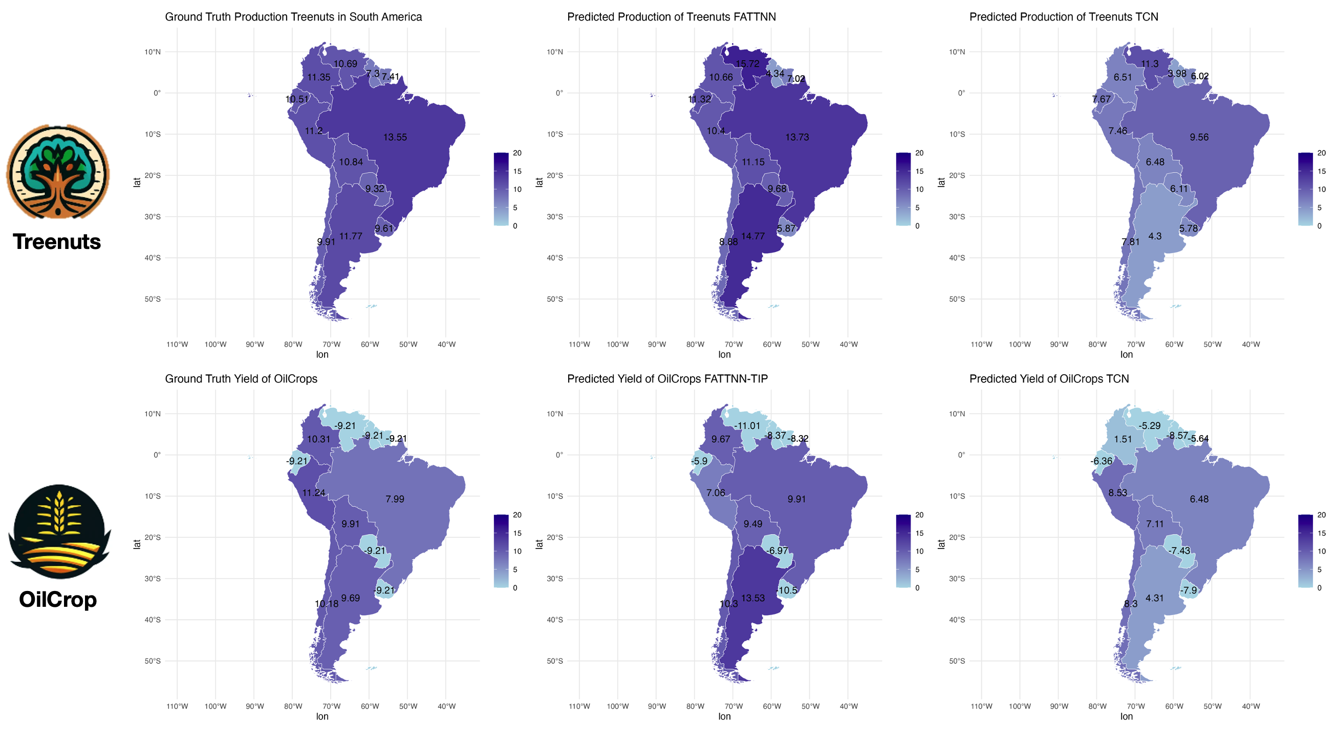
Figure 2: Comparisons between ground-truth values and predicted Production of Treenuts (top row) and Oilcrops (bottom row) in South America using the crop data of 33 countries in East Asia, North America, and Europe. Values are reported on the log-transformed scale. From left to right: Ground truth, FATTNN, and TCN.

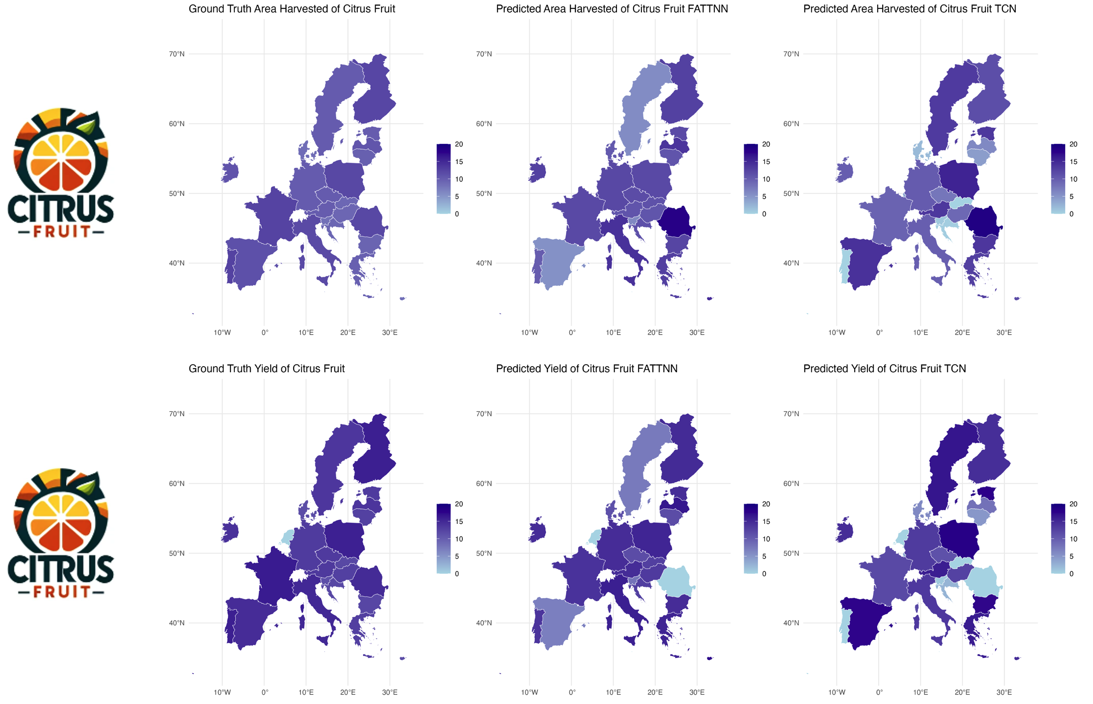
Figure 3: Comparisons between ground-truth values and predicted Yield (top row) and Area-harvested (bottom row) of citrus fruit in 26 selected countries in Europe using livestock data of the same 26 countries. Values are plotted on the log-transformed scale. For readability, numerical numbers are reported in Tables S.2 –S.3 instead of being superimposed on the plots. From left to right: Ground truth, FATTNN, and TCN.

(2) New York City (NYC) Taxi Trip Data. The data contains 24-hour taxi pick-up and drop-off information of 69 areas in New York City for all the business days in 2014 and 2015. It is publicly available at https://www.nyc.gov/site/tlc/about/tlc-trip-record-data.page. Considering the autoregressive nature of this taxi data, we include the lag-1 response as an additional covariate when fitting the models. We focus on two prediction tasks: using the pick-up and drop-off data from 6:00-14:00 to predict the pick-up and drop-off outcomes from 14:00-22:00 in 12 districts in Midtown Manhattan and 19 districts in Downtown Manhattan, respectively. A detailed Manhattan district map is provided in Figure S.1 of Appendix B. The Midtown prediction task yields a tensor covariate and response $({\cal X}_{t},{\cal Y}_{t})\in\mathbb{R}^{2\times 12\times 12\times 8}\times\mathbb{R}^{2\times 12\times 12\times 8}$ for each business day, in which the 1st dimension represents two different taxi companies, the 2nd and 3rd dimensions encode the pick-up and drop-off districts, and the 4th dimension represents the hour of day. Similarly, the Downtown prediction task involves $({\cal X}_{t},{\cal Y}_{t})\in\mathbb{R}^{2\times 19\times 19\times 8}\times\mathbb{R}^{2\times 19\times 19\times 8}$ for each business day.

From Table 4, we observe that FATTNN significantly outperforms the other approaches in terms of prediction accuracy, with a 42.5% reduction in MSE compared to TCN and a 67.6% reduction in MSE compared to Multiway in Midtown traffic prediction. In Downtown traffic prediction, FATTNN shows a 34.9% reduction in MSE compared to TCN and a 66.2% reduction in MSE compared to Multiway. As shown in the table, FATTNN is much more computationally efficient than TCN, about 6.4 times faster than TCN in Downtown prediction and 3.4 times faster in Midtown prediction. Additionally, Figure 4 visualizes the comparisons using a 5-day moving average of ground-truth values and predicted pick-up and drop-off volumes by day (where we sum the number of pick-up and drop-off across 8-hour testing periods). The FATTNN-predicted lines appear to be closer to the ground-truth lines than TCN-predicted lines in most plots.

(3) Functional Magnetic Resonance Imaging (FMRI) Data. We consider the Haxby dataset (Haxby et al.,, 2001), a well-known public dataset for research in brain imaging and cognitive neuroscience, which can be retrieved from the “NiLearn” Python library. The data contains slices of $64\times 64$ FMRI brain images collected from 1452 samples. We use the first 25 slices of each sample to predict the 26th slice of that sample, i.e., $(\mathcal{X}_{t},\mathcal{Y}_{t})\in\mathbb{R}^{25\times 64\times 64}\times\mathbb{R}^{1\times 64\times 64}$. Similar to the previous two datasets, FATTNN significantly outperforms the other methods in both prediction accuracy and computational efficiency. Compared to TCN, FATTNNyields a 46.3% reduction in MSE and computes 11 times faster. To further illustrate the algorithm performances, we visualize the predicted images in Figure 5. It is evident that FATTNN produces images that more accurately resemble the ground truth.

In summary, our proposed methods, especially the FATTNN, achieve substantial increases in prediction accuracy compared to benchmark methods – with $\sim 40\%$ reductions in MSE compared to TCN, and even larger reductions compared to Multiway Regression. At the same time, the computational costs of FATTNN methods are much lower compared to TCN which directly feeds tensor observations into a convolutional network, ranging from 2 to 11 times faster than TCN.

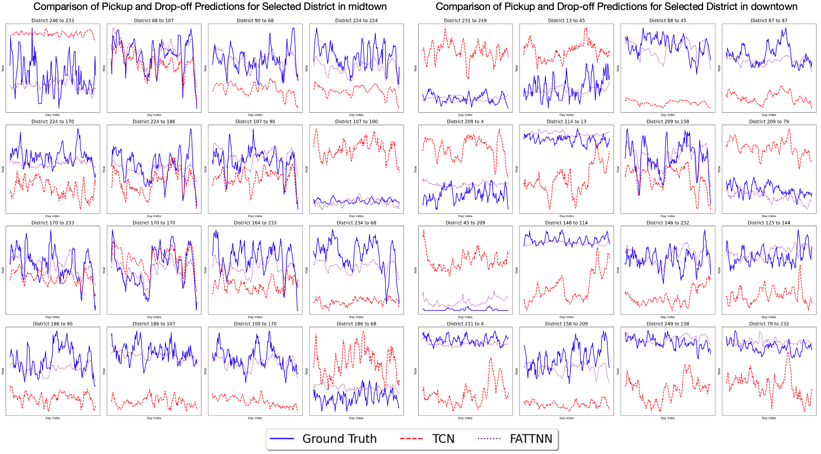
Figure 4: Comparisons between ground-truth values and predicted pick-up and drop-off volumes using various methods. “District A to B” denotes the traffic volume that passengers were picked up in District A and dropped off in District B. The district numbering is assigned according to the Manhattan district map shown in Figure S.1. Left panel: Midtown Manhattan; Right panel: Downtown Manhattan.

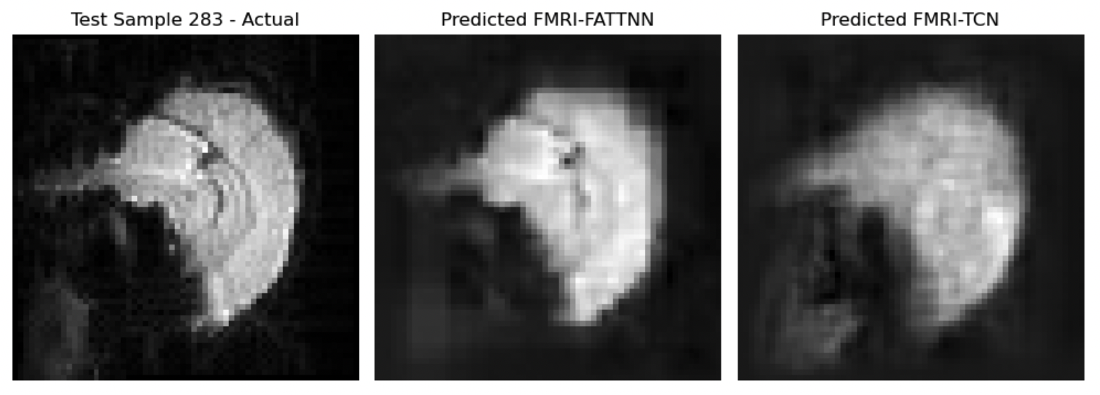
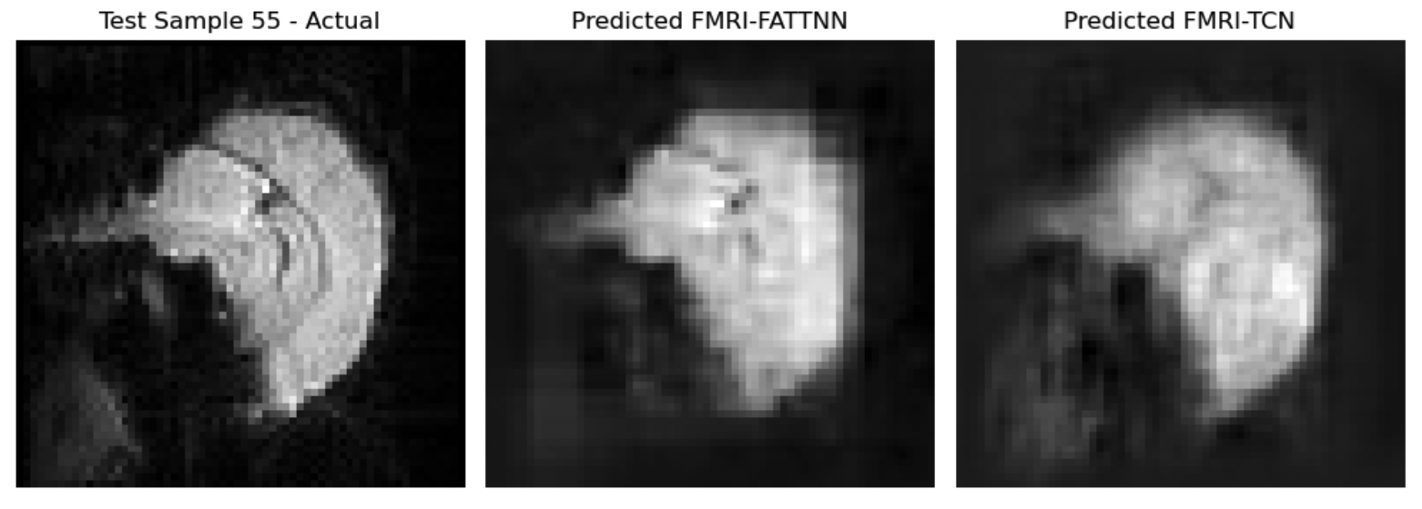
Figure 5: Comparison between ground-truth values and predicted outputs for selected samples in FMRI dataset. From left to right: Ground truth, FATTNN, and TCN.

5 Summary & Discussion

In this paper, we propose FATTNN, a hybrid method that integrates a tensor factor model into deep neural networks, for tensor-on-tensor time series forecasting. The key advantage of FATTNN is its ability to exploit and utilize the underlying tensor structure among the covariate tensors. Through a low-rank tensor factor representation, we preserve the tensor structures and, in the meantime, drastically reduce the data dimensionality, leading to enhanced prediction results and reduced computational costs. This approach unifies the strengths of both factor models and neural networks. Numerical studies confirm that our proposed methods successfully achieve substantial increases in prediction accuracy and significant reductions in computational time, compared to traditional linear tensor-on-tensor regression models (which often fail to capture the intricate nonlinearity in covariate-response relationships) and conventional deep learning approaches (that often operate in a black-box manner without intention to making use of the inherent structures among observations).

Limitations. In this work, we focus on tensor-on-tensor time series forecasting. The integration of TIPUP and TCN, both designed specifically for handling temporal data, makes our proposed approach a powerful tool for forecasting tensor series over time. When the data are not time series, the TIPUP-TCN-based FATTNN is still applicable for tensor-on-tensor prediction tasks, but the strengths of TIPUP and TCN may not be fully utilized for modeling non-temporal data. This limitation can be easily rectified by adopting proper types of tensor factor models and neural networks in the implementation of FATTNN, depending on the nature of the prediction tasks and data types involved. Please see the paragraph on generalizations of FATTNN.

Generalizations. Though we presented our models for the purpose of tensor-on-tensor time series forecasting, our proposed FATTNN framework is not confined to temporal data but can accommodate a variety of data types. The main idea of FATTNN is to use a low-rank tensor factor model to capture the intrinsic patterns among the observed covariates, and then proceed with a neural network to model the intricate relationships between covariates and responses. With appropriate choices of factor models and neural network architectures, the proposed FATTNN can be naturally adapted to any simple (e.g., i.i.d observations) or complex tensor-type data (e.g., image, graph, network, text, video). When handling time series tensors, we adopt TIPUP factorization and TCN to fully capitalize on their temporal nature. To extend beyond time series data, different types of factor models and neural network architectures should be deployed, depending on the nature of the data. For example, for graph data, Graph Neural Network is a more suitable alternative to TCN. For text data, Transformer models could substitute for the TCN in our FATTNN framework. Our proposed FATTNN is flexible in accommodating different types of tensor factor models and deep learning architecture for tensor-on-tensor prediction using diverse data types.

Appendices

Appendix A Tensor Factor Models

A.1 Notation

For a vector $x=(x_{1},...,x_{p})^{\top}$, define $\|x\|_{q}=(x_{1}^{q}+...+x_{p}^{q})^{1/q}$, $q\geq 1$. For a matrix $A=(a_{ij})\in\mathbb{R}^{m\times n}$, write the SVD as $A=U\Sigma V^{\top}$, where $\Sigma=\text{diag}(\sigma_{1}(A),\sigma_{2}(A),...,\sigma_{\min\{m,n\}}(A))$, with singular values $\sigma_{\max}(A)=$ $\sigma_{1}(A)\geq\sigma_{2}(A)\geq\cdots\geq\sigma_{\min\{m,n\}}(A)\geq 0$ in descending order. The matrix spectral norm is denoted as $\|A\|_{2}=\sigma_{1}(A).$ Write $\sigma_{\min}(A)$ the smallest nontrivial singular value of $A$. For two sequences of real numbers $\{a_{n}\}$ and $\{b_{n}\}$, write $a_{n}=O(b_{n})$ (resp. $a_{n}\asymp b_{n}$) if there exists a constant $C$ such that $|a_{n}|\leq C|b_{n}|$ (resp. $1/C\leq a_{n}/b_{n}\leq C$) for all sufficiently large $n$, and write $a_{n}=o(b_{n})$ if $\lim_{n\to\infty}a_{n}/b_{n}=0$. Write $a_{n}\lesssim b_{n}$ (resp. $a_{n}\gtrsim b_{n}$) if there exist a constant $C$ such that $a_{n}\leq Cb_{n}$ (resp. $a_{n}\geq Cb_{n}$). Write $a\wedge b=\min\{a,b\}$ and $a\vee b=\max\{a,b\}$. We use $C,C_{1},c,c_{1},...$ to denote generic constants, whose actual values may vary from line to line.

For any two $m\times r$ matrices with orthonormal columns, say, $U$ and $\widehat{U}$, suppose the singular values of $U^{\top}\widehat{U}$ are $\sigma_{1}\geq\sigma_{2}\geq\cdots\geq\sigma_{r}\geq 0$. Define the principal angles between $U$ and $\widehat{U}$ as

$$\Theta(U,\widehat{U})=\text{diag}(\arccos(\sigma_{1}),\arccos(\sigma_{2}),...,\arccos(\sigma_{r})).$$

A natural measure of distance between the column spaces of $U$ and $\widehat{U}$ is then

$$\|\widehat{U}\widehat{U}^{\top}-UU^{\top}\|_{2}=\|\sin\Theta(U,\widehat{U})\|_{2}=\sqrt{1-\sigma_{r}^{2}},$$ (S.1)

which equals to the sine of the largest principle angle between the column spaces of $U$ and $\widehat{U}$. For any two matrices $A\in\mathbb{R}^{m_{1}\times r_{1}},B\in\mathbb{R}^{m_{2}\times r_{2}}$, denote the Kronecker product $\odot$ as $A\odot B\in\mathbb{R}^{m_{1}m_{2}\times r_{1}r_{2}}$. For any two tensors ${\cal A}\in\mathbb{R}^{m_{1}\times m_{2}\times\cdots\times m_{K}},{\cal B}\in\mathbb{R}^{r_{1}\times r_{2}\times\cdots\times r_{N}}$, denote the tensor product $\otimes$ as ${\cal A}\otimes{\cal B}\in\mathbb{R}^{m_{1}\times\cdots\times m_{K}\times r_{1}\times\cdots\times r_{N}}$, such that

$$({\cal A}\otimes{\cal B})_{i_{1},...,i_{K},j_{1},...,j_{N}}=({\cal A})_{i_{1},...,i_{K}}({\cal B})_{j_{1},...,j_{N}}.$$

Let ${\rm{vec}}(\cdot)$ be the vectorization of matrices and tensors. The mode-$k$ unfolding (or matricization) is defined as ${\rm{mat}}_{k}({\cal A})$, which maps a tensor ${\cal A}$ to a matrix ${\rm{mat}}_{k}({\cal A})\in\mathbb{R}^{m_{k}\times m_{-k}}$ where $m_{-k}=\prod_{j\neq k}^{K}m_{j}$. For example, if ${\cal A}\in\mathbb{R}^{m_{1}\times m_{2}\times m_{3}}$, then

$$({\rm{mat}}_{1}({\cal A}))_{i,(j+m_{2}(k-1))}=({\rm{mat}}_{2}({\cal A}))_{j,(k+m_{3}(i-1))}=({\rm{mat}}_{3}({\cal A}))_{k,(i+m_{1}(j-1))}={\cal A}_{ijk}.$$

For tensor ${\cal A}\in\mathbb{R}^{m_{1}\times m_{2}\times\cdots\times m_{K}}$, the Hilbert Schmidt norm or Frobenius norm is defined as

$$\|{\cal A}\|_{{\rm F}}=\sqrt{\sum_{i_{1}=1}^{m_{1}}\cdots\sum_{i_{K}=1}^{m_{K}}({\cal A})_{i_{1},...,i_{K}}^{2}}.$$

A.2 Preliminary of matrix and tensor algebra

Fact (Norm inequalities).

• For any matrix $A,B$, $\|AB\|\geq\|A\|\cdot\sigma_{\min}(B)$.

• For any matrix $A$, square invertible matrix $B$, $\|A\|\leq\sigma_{\max}(B)\cdot\|AB^{-1}\|$.

• For any matrix $A$, and square diagonal invertible matrix $B$, $\sigma_{\min}(BA)\geq\sigma_{\min}(B)\cdot\sigma_{\min}(A)$.

Lemma A.1 (Weyl’s inequality).

Let $A,B\in\mathbb{R}^{m\times n}$ where $n\geq k$, then we have for any $i\in[k]$,

$$|\sigma_{i}(A)-\sigma_{i}(B)|\leq\|A-B\|\$$ (S.2)

Lemma A.2 (Davis–Kahan $\sin\Theta$ theorem).

Let $\Sigma,\hat{\Sigma}\in\mathbb{R}^{p\times p}$ be symmetric, with eigenvalues $\lambda_{1}\geq\cdots\geq\lambda_{p}$ and $\hat{\lambda}_{1}\geq\cdots\geq\hat{\lambda}_{p}$ respectively. Fix $1\leq r\leq s\leq p$, let $d=s-r+1$, and let $V=(v_{r},v_{r+1},\ldots,v_{s})\in\mathbb{R}^{p\times d}$ and $\hat{V}=(\hat{v}_{r},\hat{v}_{r+1},\ldots,\hat{v}_{s})\in\mathbb{R}^{p\times d}$ have orthonormal columns satisfying $\Sigma v_{j}=\lambda_{j}v_{j}$ and $\hat{\Sigma}\hat{v}_{j}=\hat{\lambda}_{j}\hat{v}_{j}$ for $j=r,r+1,\ldots,s$. Write $\delta=\inf\{|\hat{\lambda}-\lambda|:\lambda\in[\lambda_{s},\lambda_{r}],\hat{\lambda}\in(-\infty,\hat{\lambda}_{s+1}]\cup[\hat{\lambda}_{r-1},\infty)\}$, where we define $\hat{\lambda}_{0}=-\infty$ and $\hat{\lambda}_{p+1}=\infty$, and assume that $\delta>0$. Then

$$\|\sin\Theta(\hat{V},V)\|\leq\frac{\|\hat{\Sigma}-\Sigma\|}{\delta},$$ (S.3)

where the norm $\|\cdot\|$ could be spectral norm $\|\cdot\|_{2}$ or Frobenious norm $\|\cdot\|_{\rm F}$. Frequently in applications, we have $r=s=j$, say, in which case we have

$$\|\sin\Theta(\hat{v}_{j},v_{j})\|_{2}\leq\frac{\|\hat{\Sigma}-\Sigma\|_{2}}{\min(|\hat{\lambda}_{j-1}-\lambda_{j}|,|\hat{\lambda}_{j+1}-\lambda_{j}|)}.$$ (S.4)

A.3 Technical lemmas

Lemma A.3 ($\epsilon$-covering of matrix norms, Han et al., (2020)).

Let $d,d_{j},d_{*},r\leq d\wedge d_{j}$ be positive integers, $\epsilon>0$ and $N_{d,\epsilon}=\lfloor(1+2/\epsilon)^{d}\rfloor$.
(i) For any norm $\|\cdot\|$ in $\mathbb{R}^{d}$, there exist $M_{j}\in\mathbb{R}^{d}$ with $\|M_{j}\|\leq 1$, $j=1,\ldots,N_{d,\epsilon}$, such that $\max_{\|M\|\leq 1}\min_{1\leq j\leq N_{d,\epsilon}}\|M-M_{j}\|\leq\epsilon$. Consequently, for any linear mapping $f$ and norm $\|\cdot\|_{*}$,

$$\sup_{M\in\mathbb{R}^{d},\|M\|\leq 1}\|f(M)\|_{*}\leq 2\max_{1\leq j\leq N_{d,1/2}}\|f(M_{j})\|_{*}.$$

(ii) Given $\epsilon>0$, there exist $U_{j}\in\mathbb{R}^{d\times r}$ and $V_{j^{\prime}}\in\mathbb{R}^{d^{\prime}\times r}$ with $\|U_{j}\|_{2}\vee\|V_{j^{\prime}}\|_{2}\leq 1$ such that

$$\max_{M\in\mathbb{R}^{d\times d^{\prime}},\|M\|_{2}\leq 1,\text{rank}(M)\leq r}\ \min_{j\leq N_{dr,\epsilon/2},j^{\prime}\leq N_{d^{\prime}r,\epsilon/2}}\|M-U_{j}V_{j^{\prime}}^{\top}\|_{2}\leq\epsilon.$$

Consequently, for any linear mapping $f$ and norm $\|\cdot\|_{*}$ in the range of $f$,

$$\sup_{M,\widetilde{M}\in\mathbb{R}^{d\times d^{\prime}},\|M-\widetilde{M}\|_{2}\leq\epsilon\atop{\|M\|_{2}\vee\|\widetilde{M}\|_{2}\leq 1\atop\text{rank}(M)\vee\text{rank}(\widetilde{M})\leq r}}\frac{\|f(M-\widetilde{M})\|_{*}}{\epsilon 2^{I_{r<d\wedge d^{\prime}}}}\leq\sup_{\|M\|_{2}\leq 1\atop\text{rank}(M)\leq r}\|f(M)\|_{*}\leq 2\max_{1\leq j\leq N_{dr,1/8}\atop 1\leq j^{\prime}\leq N_{d^{\prime}r,1/8}}\|f(U_{j}V_{j^{\prime}}^{\top})\|_{*}.$$ (S.5)

(iii) Given $\epsilon>0$, there exist $U_{j,k}\in\mathbb{R}^{d_{k}\times r_{k}}$ and $V_{j^{\prime},k}\in\mathbb{R}^{d^{\prime}_{k}\times r_{k}}$ with $\|U_{j,k}\|_{2}\vee\|V_{j^{\prime},k}\|_{2}\leq 1$ such that

$$\max_{M_{k}\in\mathbb{R}^{d_{k}\times d_{k}^{\prime}},\|M_{k}\|_{2}\leq 1\atop\text{rank}(M_{k})\leq r_{k},\forall k\leq K}\ \min_{j_{k}\leq N_{d_{k}r_{k},\epsilon/2}\atop j^{\prime}_{k}\leq N_{d_{k}^{\prime}r_{k},\epsilon/2},\forall k\leq K}\Big{\|}\odot_{k=2}^{K}M_{k}-\odot_{k=2}^{K}(U_{j_{k},k}V_{j_{k}^{\prime},k}^{\top})\Big{\|}_{\rm op}\leq\epsilon(K-1).$$

For any linear mapping $f$ and norm $\|\cdot\|_{*}$ in the range of $f$,

$$\sup_{M_{k},\widetilde{M}_{k}\in\mathbb{R}^{d_{k}\times d_{k}^{\prime}},\|M_{k}-\widetilde{M}_{k}\|_{2}\leq\epsilon\atop{\text{rank}(M_{k})\vee\text{rank}(\widetilde{M}_{k})\leq r_{k}\atop\|M_{k}\|_{2}\vee\|\widetilde{M}_{k}\|_{2}\leq 1\ \forall k\leq K}}\frac{\|f(\odot_{k=2}^{K}M_{k}-\odot_{k=2}^{K}\widetilde{M}_{k})\|_{*}}{\epsilon(2K-2)}\leq\sup_{M_{k}\in\mathbb{R}^{d_{k}\times d_{k}^{\prime}}\atop{\text{rank}(M_{k})\leq r_{k}\atop\|M_{k}\|_{2}\leq 1,\forall k}}\Big{\|}f\big{(}\odot_{k=2}^{K}M_{k}\big{)}\Big{\|}_{*}$$ (S.6)

and

$$\sup_{M_{k}\in\mathbb{R}^{d_{k}\times d_{k}^{\prime}},\|M_{k}\|_{2}\leq 1\atop\text{rank}(M_{k})\leq r_{k}\ \forall k\leq K}\Big{\|}f\big{(}\odot_{k=2}^{K}M_{k}\big{)}\Big{\|}_{*}\leq 2\max_{1\leq j_{k}\leq N_{d_{k}r_{k},1/(8K-8)}\atop 1\leq j_{k}^{\prime}\leq N_{d_{k}^{\prime}r_{k},1/(8K-8)}}\Big{\|}f\big{(}\odot_{k=2}^{K}U_{j_{k},k}V_{j_{k}^{\prime},k}^{\top}\big{)}\Big{\|}_{*}.$$ (S.7)

Lemma A.4 (Slepian’s inequality, Vershynin, (2018)).

Let $(X_{t})_{t\in T}$ and $(Y_{t})_{t\in T}\in T$ be two mean zero Gaussian Processes. Assume that for all $t,s\in T$, we have

$$\mathbb{E}X_{t}^{2}=\mathbb{E}Y_{t}^{2}\quad\text{and}\quad\mathbb{E}[(X_{t}-X_{s})^{2}]\leq\mathbb{E}[(Y_{t}-Y_{s})^{2}].$$ (S.8)

Then for every $\tau\in R$, we have

$$\mathbb{P}\left\{\sup_{t\in T}X_{t}\geq\tau\right\}\leq\mathbb{P}\left\{\sup_{t\in T}Y_{t}\geq\tau\right\}.$$ (S.9)

Consequently,

$$\mathbb{E}\sup_{t\in T}X_{t}\leq\mathbb{E}\sup_{t\in T}Y_{t}$$ (S.10)

Lemma A.5 (Sudakov-Fernique inequality, Vershynin, (2018)).

Let $(X_{t})_{t\in T}$ and $(Y_{t})_{t\in T}$ be two mean-zero Gaussian processes. Assume that, for all $t,s\in T$, we have

$$\mathbb{E}[(X_{t}-X_{s})^{2}]\leq\mathbb{E}[(Y_{t}-Y_{s})^{2}].$$ (S.11)

Then,

$$\mathbb{E}\left[\sup_{t\in T}\{X_{t}\}\right]\leq\mathbb{E}\left[\sup_{t\in T}\{Y_{t}\}\right].$$ (S.12)

A function $f:\mathbb{R}^{d}\to\mathbb{R}$ is $L$-Lipschitz continuous (sometimes called globally Lipschitz continuous) if there exists $L\in\mathbb{R}$ such that

$$\|f(x)-f(y)\|\leq L\|x-y\|.$$

The smallest constant $L>0$ is denoted $\|f\|_{\rm Lip}$.

Lemma A.6 (Gaussian Concentration of Lipschitz functions, Vershynin, (2018)).

Let $X\sim N(0,I_{d})$ and let $f:\mathbb{R}^{d}\to\mathbb{R}$ be a Lipschitz function. Then,

$$\mathbb{P}\left(f(X)-\mathbb{E}f(X)\geq t\right)\leq 2\exp\left(-\frac{t^{2}}{2\|f\|_{\rm Lip}}\right).$$

Lemma A.7 (Sigular values of Gaussian random matrices).

Let $X$ be an $n\times p$ matrix with i.i.d. $N(0,1)$ entries. For any $x>0$,

$$\mathbb{P}\left(\left\|X^{\top}X-nI_{p}\right\|_{2}\geq p+2\sqrt{pn}+2x(\sqrt{p}+\sqrt{n})+x^{2}\right)\leq 2e^{-x^{2}/2}.$$

Proof.

It can be easily derived by Corollary 5.35 in Vershynin, (2010). ∎

A.4 The Determination of Rank

Here, the estimators are constructed with given ranks $r_{1},\ldots,r_{K}$. Determining the number of factors in a data-driven manner has been a significant research topic in the factor model literature. Recently, Han et al., (2022) established a class of rank determination approaches for tensor factor models, based on both the information criterion and the eigen-ratio criterion. These procedures can be adopted for our purposes.

A.5 Tucker Decomposition and iterative TIPUP (iTIPUP) Algorithm

The Higher-Order Orthogonal Iteration (HOOI) algorithm De Lathauwer et al., (2000) is one of the most popular methods for computing the Tucker decomposition, which relies on the orthogonal projection and Singular Value Decomposition (SVD) to update the estimation of loading matrices for each tensor mode in every iteration.

Similar to the idea of HOOI, an iterative refinement version of TIPUP could further improve its performance, just as HOOI enhances the original Tucker decomposition method. The pseudo-code for this iterative refinement is provided in Algorithm S.1.

Algorithm S.1 Iterative TIPUP (iTIPUP) algorithm

1:  Input: $\mathcal{X}_{t}\in\mathbb{R}^{d_{1}\times\ldots\times d_{K}}$ for $t=1,\ldots,n$, rank $r_{k}$ for all $k=1,\ldots,K$, the tolerance parameter $\epsilon>0$, the maximum number of iterations $J$.

2:  Let $j=0$, initiate via TIPUP on ${\cal X}_{1},...,{\cal X}_{n}$ to obtain

$$\widehat{A}_{k}^{(0)}=\text{LSVD}_{r_{k}}\left(\frac{1}{n}\sum_{t=1}^{n}\hbox{\rm mat}_{k}({\cal X}_{t})\hbox{\rm mat}_{k}^{\top}({\cal X}_{t})\right),$$

where LSVD${}_{r_{k}}$ stands for the top $r_{k}$ left singular vectors, $k=1,...,K$.

3:  repeat

4:     Let $j=j+1$.

5:     for $k=1,\ldots,K$ do

6:        Given previous estimates $\widehat{A}_{1}^{(j-1)},\ldots,\widehat{A}_{k-1}^{(j-1)},\widehat{A}_{k+1}^{(j-1)},\ldots,\widehat{A}_{K}^{(j-1)}$, sequentially calculate,

$$Z_{t,k}^{(j)}={\cal X}_{t}\times_{1}\widehat{A}_{1}^{(j)\top}\times_{2}\ldots\times_{k-1}\widehat{A}_{k-1}^{(j)\top}\times_{k+1}\widehat{A}_{k+1}^{(j-1)\top}\times_{k+2}\ldots\times_{K}\widehat{A}_{K}^{(j-1)\top},$$

for $t=1,\ldots,n$.

7:        Perform TIPUP on the new tensor series $(Z_{1,k}^{(j)},\ldots,Z_{n,k}^{(j)})$,

$$\widehat{A}_{k}^{(j)}=\text{LSVD}_{r_{k}}\left(\frac{1}{n}\sum_{t=1}^{n}\hbox{\rm mat}_{k}(Z_{t,k}^{(j)})\hbox{\rm mat}_{k}^{\top}(Z_{t,k}^{(j)})\right).$$

8:     end for

9:  until $j=J$ or $\max_{1\leq k\leq K}\|\widehat{A}_{k}^{(j)}\widehat{A}_{k}^{(j)\top}-\widehat{A}_{k}^{(j-1)}\widehat{A}_{k}^{(j-1)\top}\|_{2}\leq\epsilon$.

10:  Output:

$$\widehat{A}_{k} =\widehat{A}_{k}^{(j)},\quad k=1,\ldots,K,$$

$$\widehat{F}_{t} =\mathcal{X}_{t}\times_{k=1}^{K}\widehat{A}_{K}^{\top},\quad t=1,\ldots,n.$$

A.6 Proof of Proposition 3.1

We focus on the case of $K=2$ as the iTIPUP begins with mode-$k$ matrix unfolding. In particular, we sometimes give explicit expressions only in the case of $k=1$ and $K=2$. For $K=2$, we observe a matrix time series with $X_{t}=A_{1}F_{t}A_{2}^{\top}+{\cal E}_{t}\in\mathbb{R}^{d_{1}\times d_{2}}$. Let $\overline{\mathbb{E}}(\cdot)=\mathbb{E}(\cdot|\{{\cal F}_{1},...,{\cal F}_{n}\})$ and $\overline{\mathbb{P}}(\cdot)=\mathbb{P}(\cdot|\{{\cal F}_{1},...,{\cal F}_{n}\})$.

Let $L_{k}^{(m)}$ be the loss for $\hat{A}_{k}^{(m)}$ at the $m$-th iteration,

$$L_{k}^{(m)}=\|\widehat{P}_{k}^{(m)}-P_{k}\|_{2},\quad L^{(m)}=\max_{1\leq k\leq K}L_{k}^{(m)},$$

where $\widehat{P}_{k}^{(m)}=A_{k}^{(m)}(A_{k}^{(m)\top}A_{k}^{(m)})^{-1}A_{k}^{(m)^{\top}}$.

We outline the proof as follows.

(i) Initialization.

Define

$${\rm TIPUP}_{1}=\frac{1}{n}\sum_{t=1}^{n}X_{t}X_{t}^{\top}\in\mathbb{R}^{d_{1}\times d_{1}},$$

The “noiseles” version of TIPUP₁ is

$$\Theta_{1}=\frac{1}{n}\sum_{t=1}^{n}A_{1}F_{t}A_{2}^{\top}A_{2}F_{1}^{\top}A_{1}^{\top}\in\mathbb{R}^{d_{1}\times d_{1}},$$

which is of rank $r_{1}$. Then, by Davis-Kahan sin $\Theta$ theorem (Lemma A.2),

$$L_{1}^{(0)}=\|P_{1}-\widehat{P}_{1}^{(0)}\|_{2}\leq\frac{2\|{\rm TIPUP}_{1}-\Theta_{1}\|_{2}}{\sigma_{r_{1}}(\Theta_{1})}.$$ (S.13)

To bound the numerator on the right hand side of (S.13), we write

$${\rm TIPUP}_{1}-\Theta_{1}=\frac{1}{n}\sum_{t=1}^{n}A_{1}F_{t}A_{2}^{\top}{\cal E}_{t}^{\top}+\frac{1}{n}\sum_{t=1}^{n}{\cal E}_{t}A_{2}{\cal F}_{t}^{\top}A_{1}^{\top}+\frac{1}{n}\sum_{t=1}^{n}{\cal E}_{t}{\cal E}_{t}^{\top}:=\Delta_{1}+\Delta_{2}+\Delta_{3}.$$

For $\Delta_{3}$, by Lemma A.7,

$$\mathbb{P}\left(\left\|\sum_{t=1}^{n}\mathcal{E}_{t}\mathcal{E}_{t}^{\top}-n\mathbb{E}\mathcal{E}_{t}\mathcal{E}_{t}^{\top}\right\|_{2}\geq d_{1}+2\sqrt{d_{1}d_{2}n}+2x(\sqrt{d_{1}}+\sqrt{d_{2}n})+x^{2}\right)\leq 2e^{-x^{2}/2}.$$

By setting $x\asymp\sqrt{d_{1}}$, with probability at least $1-e^{-d_{1}}$,

$$\left\|\Delta_{3}-\mathbb{E}\mathcal{E}_{t}\mathcal{E}_{t}^{\top}\right\|_{2}\lesssim\frac{d_{1}}{n}+\sqrt{\frac{d_{1}d_{2}}{n}}.$$

Next consider $\Delta_{1}$ and $\Delta_{2}$. For any $u$ and $v$ in $\mathbb{R}^{d_{1}}$, we have

$$\overline{\mathbb{E}}\left(u^{\top}\left(\frac{1}{\sqrt{n}}\sum_{t=1}^{n}A_{1}F_{t}A_{2}^{\top}\mathcal{E}_{t}^{\top}\right)v\right)^{2}\leq\|\Theta_{1}\|_{2}\|u\|_{2}^{2}\|v\|_{2}^{2}.$$

Thus for $u_{i}$ and $v_{i}$ with $\|u_{i}\|_{2}=\|v_{i}\|_{2}=1$, $i=1,2$,

$$n\|\Theta_{1}\|_{2}^{-1}\overline{\mathbb{E}}\left((u_{1}^{\top}\Delta_{1}v_{1}-u_{2}^{\top}\Delta_{1}v_{2})^{2}\right) \leq\left(\|u_{1}-u_{2}\|_{2}\|v_{1}\|_{2}+\|u_{2}\|_{2}\|v_{1}-v_{2}\|_{2}\right)^{2}$$

$$\leq 2\left(\|u_{1}-u_{2}\|_{2}^{2}+\|v_{1}-v_{2}\|_{2}^{2}\right)$$

$$=2\mathbb{E}\left[(u_{1}-u_{2})^{\top}\xi+(v_{1}-v_{2})^{\top}\zeta\right]^{2},$$

where $\xi$ and $\zeta$ are i.i.d $N(0,I_{d_{1}})$ vectors. As $\Delta_{1}$ is a $d_{1}\times d_{1}$ Gaussian matrix under $\overline{\mathbb{E}}$, the Sudakov-Fernique inequality (Lemma A.5) yields

$$\sqrt{n}\|\Theta_{1}\|_{2}^{-1/2}\overline{\mathbb{E}}\|\Delta_{1}\|_{2}\leq\sqrt{2}\mathbb{E}\sup_{\|u\|_{2}=\|v\|_{2}=1}(u^{\top}\xi+v^{\top}\zeta)=\sqrt{2}\mathbb{E}\left(\|\xi\|_{2}+\|\zeta\|_{2}\right)\leq 2\sqrt{2d_{1}}.$$

It follows that

$$\overline{\mathbb{E}}\|\Delta_{1}\|_{2}\leq\sqrt{\frac{8d_{1}}{n}}\|\Theta_{1}\|_{2}^{1/2}.$$

Elementary calculation shows that $\|\Delta_{1}\|_{2}$ is a $\sqrt{n}\|\Theta_{1}\|_{2}^{1/2}$-Lipschitz function. Then, by Gaussian concentration inequality for Lipschitz functions (Lemma A.6),

$$\overline{\mathbb{P}}\left(\|\Delta_{1}\|_{2}\geq\sqrt{\frac{8d_{1}}{n}}\|\Theta_{1}\|_{2}^{1/2}+\sqrt{\frac{1}{n}}\|\Theta_{1}\|_{2}^{1/2}x\right)\leq 2e^{-\frac{x^{2}}{2}}.$$

With $x\asymp\sqrt{d_{1}}$, with probability at least $1-e^{-d_{1}}$,

$$\|\Delta_{2}\|_{2}=\|\Delta_{1}\|_{2}\lesssim\sqrt{\frac{d_{1}}{n}}\sigma_{1}(\Theta_{1}).$$

As $\sigma_{1}(\Theta_{1})=\sigma_{r_{1}}(\Theta_{1})\asymp\lambda^{2}$, by (S.13), with probability at least $1-e^{-d_{1}}$,

$$L_{1}^{(0)}=\|\widehat{P}_{1}^{(0)}-P_{1}\|_{2}\lesssim\frac{1}{\lambda^{2}}\sqrt{\frac{d}{n}}+\frac{d_{1}}{\lambda^{2}n}+\frac{1}{\lambda}\sqrt{\frac{d_{1}}{n}}.$$ (S.14)

(ii) Iterative refinement.

After the initialization with $\widehat{A}_{k}^{(0)}$, the algorithm iteratively produces estimates $\widehat{A}_{k}^{(m)}$ from $m=1$ to $m=J$. Define the matrix-valued operator TIPUP${}_{1}(\cdot)$ as

$${\rm TIPUP_{1}}(U_{2})=\frac{1}{n}\sum_{t=1}^{n}X_{t}U_{2}U_{2}^{\top}X_{t}^{\top}\in\mathbb{R}^{d_{2}\times d_{2}},$$

for any matrix-valued variable $U_{2}\in\mathbb{R}^{d_{2}\times r_{2}}$. Given $\widehat{A}_{2}^{(m)}$, the $(m+1)$-th iteration produces estimates

$$\widehat{A}_{1}^{(m+1)}=\text{LSVD}_{r_{1}}(\text{TIPUP}_{1}(\widehat{A}_{2}^{(m)})),\quad\widehat{P}_{1}^{(m+1)}=\widehat{A}_{1}^{(m+1)}\widehat{A}_{1}^{(m+1)^{\top}}.$$ (S.15)

The “noiseless” version of this update is given by

$$\Theta_{1}(U_{2})=\frac{1}{n}\sum_{t=1}^{n}A_{1}F_{t}A_{2}^{\top}U_{2}U_{2}^{\top}A_{2}F_{t}^{\top}A_{1}^{\top}=\Theta_{1}$$

giving error-free “estimates”,

$$\widehat{A}_{1}^{(m+1)}=\text{LSVD}_{r_{1}}(\Theta_{1}(\widehat{A}_{2}^{(m)})),$$

where $\Theta_{1}(\widehat{A}_{2}^{(m)})$ is of rank $r_{1}$. Thus, by Davis-Kahan sin $\Theta$ theorem (Lemma A.2)

$$L_{1}^{(m+1)}=\|\widehat{P}_{1}^{(m+1)}-P_{1}\|_{2}\leq\frac{2\|\text{TIPUP}_{1}(\widehat{A}_{2}^{(m)})-\Theta_{1}(\widehat{A}_{2}^{(m)})\|_{2}}{\sigma_{r_{1}}[\Theta_{1}(\widehat{A}_{2}^{(m)})]}.$$ (S.16)

To bound the numerator on the right-hand side of (S.16), we write

$$\text{TIPUP}_{1}(U_{2})-\Theta_{1}(U_{2}):=\Delta_{1}(U_{2}U_{2}^{\top})+\Delta_{2}(U_{2}U_{2}^{\top})+\Delta_{3}(U_{2}U_{2}^{\top}),$$

where for any $M_{2}\in\mathbb{R}^{d_{2}\times d_{2}}$,

$$\Delta_{1}(M_{2}) =\frac{1}{n}\sum_{t=1}^{n}A_{1}F_{t}A_{2}^{\top}M_{2}\mathcal{E}_{t}^{\top},$$

$$\Delta_{2}(M_{2}) =\frac{1}{n}\sum_{t=1}^{n}\mathcal{E}_{t}M_{2}A_{2}F_{t}^{\top}A_{1}^{\top},$$

$$\Delta_{3}(M_{2}) =\frac{1}{n}\sum_{t=1}^{n}\mathcal{E}_{t}M_{2}\mathcal{E}_{t}^{\top}.$$

As $\Delta_{i}(M_{2})$ is linear in $M_{2}$, the numerator on the right-hand side of (S.16) can be bounded by

$$\|\text{TIPUP}_{1}(\widehat{A}_{2}^{(m)})-\Theta_{1}(\widehat{A}_{2}^{(m)})\|_{2}\leq\|\text{TIPUP}_{1}(A_{2})-\Theta_{1}(A_{2})\|_{2}+L^{(m)}(2K-2)\sum_{i=1}^{3}\|\Delta_{i}(M_{2})\|_{\rm S},$$

where

$$\|\Delta_{i}(M_{2})\|_{\rm S}=\max_{\|M_{2}\|_{1}\leq 1,\text{rank}(M_{2})\leq r_{2}}\|\Delta_{i}(M_{2})\|_{2}.$$

We claim in certain events $\Omega_{i}$, with $\mathbb{P}(\Omega_{i})\geq 1-e^{-d_{1}}$,

$$\|\Delta_{i}(M_{2})\|_{\rm S} \lesssim\sqrt{\frac{d_{1}+d_{2}}{n}}\lambda,\quad i=1,2,$$ (S.17)

$$\|\Delta_{3}(M_{2})\|_{\rm S} \lesssim\frac{d_{1}+d_{2}}{n}+\sqrt{\frac{d_{1}+d_{2}}{n}}.$$ (S.18)

We will also prove by induction, the denominator in (S.16) satisfies

$$2\sigma_{r_{1}}[\Theta_{1}(\widehat{A}_{2}^{(m)})]\geq\sigma_{r_{1}}[\Theta_{1}(A_{2})].$$ (S.19)

Define the ideal version of the ratio in (S.16) as

$$L_{k}^{(\text{ideal})}=\frac{\|\text{TIPUP}_{1}(\odot_{j\neq k}A_{j})-\Theta_{k}(\odot_{j\neq k}A_{j})\|_{2}}{\sigma_{r_{1}}[\Theta_{k}(\odot_{j\neq k}A_{j})]},\quad L^{(\text{ideal})}=\max_{1\leq k\leq K}L_{k}^{(\text{ideal})}.$$

The proof of (S.17) and (S.18) implies that, in an event with probability at least $1-\frac{k}{2}e^{-d_{k}}$,

$$L_{k}^{(\text{ideal})}\lesssim\frac{1}{\lambda^{2}}\sqrt{\frac{d_{k}}{n}}+\frac{d_{k}}{\lambda^{2}n}+\frac{1}{\lambda}\sqrt{\frac{d_{k}}{n}}.$$ (S.20)

Putting together (S.13),(S.14),(S.16),(S.17),(S.18) and (S.19), we have

$$L_{k}^{(m+1)}\leq L_{k}^{(\text{ideal})}+L^{(m)}\rho,$$

with $\rho<1$. By induction,

$$L^{(m+1)}\leq(1+\rho+\dots+\rho^{m})L^{(m)}+\rho^{m+1}L^{(0)}.$$

We achieve the desired results.

We divided the rest of the proof into 4 steps to prove (S.17) and (S.18)for $i=1,2,3$ and (S.19).

Step 1.

We prove (S.17) for the $\|\Delta_{1}(M_{2})\|_{\rm S}$.

By Lemma A.3 (ii), there exists $\widetilde{M}^{(\ell,\ell^{\prime})}\in\mathbb{R}^{d_{2}\times d_{2}}$ of the forms $W_{\ell}Q_{\ell^{\prime}}^{\top}$ with $W_{\ell}\in\mathbb{R}^{d_{2}\times r_{2}}$, $Q_{\ell^{\prime}}\in\mathbb{R}^{d_{2}\times r_{2}}$, $1\leq\ell,\ell^{\prime}\leq N_{d_{2}r_{2},1/8}=17^{d_{2}r_{2}}$, such that $\|\widetilde{M}^{(\ell,\ell^{\prime})}\|_{2}\leq 1$, $\text{rank}(\widetilde{M}^{(\ell,\ell^{\prime})})\leq r_{2}$ and

$$\|\Delta_{1}(M_{2})\|_{\rm S}\leq 2\max_{\ell,\ell^{\prime}\leq N_{d_{2}r_{2},1/8}}\left\|\frac{1}{n}\sum_{t=1}^{n}A_{1}F_{t}A_{2}^{\top}\widetilde{M}^{(\ell,\ell^{\prime})}\mathcal{E}_{t}^{\top}\right\|_{2}.$$

Elementary calculation shows that $\|\Delta_{1}(\widetilde{M}^{(\ell,\ell^{\prime})})\|_{2}$ is a $\sqrt{n}\|\Theta_{1}\|_{2}$-Lipschitz function of $\mathcal{E}_{1},\ldots,\mathcal{E}_{n}$. Employing similar argument as the initialization (Sudakov-Fernique inequality, Lemma A.5), we have

$$\overline{\mathbb{E}}\left\|\frac{1}{n}\sum_{t=1}^{n}A_{1}F_{t}A_{2}^{\top}\widetilde{M}^{(\ell,\ell^{\prime})}\mathcal{E}_{t}^{\top}\right\|_{2}\leq\sqrt{\frac{8d_{1}}{n}}\|\Theta_{1}\|_{2}^{1/2}.$$

Then, by Gaussian concentration inequality for Lipschitz functions (Lemma A.6),

$$\overline{\mathbb{P}}\left(\left\|\frac{1}{n}\sum_{t=1}^{n}A_{1}F_{t}A_{2}^{\top}\widetilde{M}^{(\ell,\ell^{\prime})}\mathcal{E}_{t}^{\top}\right\|_{2}-\sqrt{\frac{8d_{1}}{n}}\|\Theta_{1}\|_{2}^{1/2}\geq\frac{1}{\sqrt{n}}\|\Theta_{1}\|_{2}^{1/2}x\right)\leq e^{-x^{2}/2}.$$

Hence,

$$\overline{\mathbb{P}}\left(\|\Delta_{1}(M_{2})\|_{\rm S}\geq\sqrt{\frac{8d_{1}}{n}}\|\Theta_{1}\|_{2}^{1/2}+\frac{1}{\sqrt{n}}\|\Theta_{1}\|_{2}^{1/2}x\right)\leq N_{d_{2}r_{2},1/8}^{2}e^{-x^{2}/2}.$$

This implies that with $x\asymp\sqrt{d_{2}r_{2}}$ that in an event with probability at least $1-e^{-d_{2}}$,

$$\|\Delta_{1}(M_{2})\|_{\rm S}\lesssim\sqrt{\frac{d_{1}+d_{2}r_{2}}{n}}\lambda\lesssim\sqrt{\frac{d_{1}+d_{2}}{n}}\lambda.$$

Step 2.

The bound of $\|\Delta_{2}(M_{2})\|_{\rm S}$ follows from the same argument as the above step.

Step 3.

Here we prove (S.18) for $\|\Delta_{3}(M_{2})\|_{\rm S}$. By Lemma A.3(iii), we can find $U_{2}^{(\ell)}\in\mathbb{R}^{d_{2}\times r_{2}}$, $1\leq\ell\leq N_{d_{2}r_{2},1/8}$ such that $\|U_{2}^{(\ell)}\|_{2}\leq 1$ and

$$\|\Delta_{3}(M_{2})\|_{\rm S}\leq 2\max_{1\leq\ell\leq N_{d_{2}r_{2},1/8}}\left\|\frac{1}{n}\sum_{t=1}^{n}\mathcal{E}_{t}U_{2}^{(\ell)}U_{2}^{(\ell)\top}\mathcal{E}_{t}^{\top}\right\|_{2}.$$

By Lemma A.7,

$$\mathbb{P}\left(\left\|\sum_{t=1}^{n}\mathcal{E}_{t}U_{2}^{(\ell)}U_{2}^{(\ell)\top}\mathcal{E}_{t}^{\top}-n\mathbb{E}\mathcal{E}_{t}U_{2}^{(\ell)}U_{2}^{(\ell)\top}\mathcal{E}_{t}^{\top}\right\|_{2}\geq d_{1}+2\sqrt{d_{1}r_{2}n}+2x(\sqrt{d_{1}}+\sqrt{r_{2}n})+x^{2}\right)\leq 2e^{-x^{2}/2}.$$

Hence, by setting $x\asymp\sqrt{d_{2}r_{2}}$, we have with probability at least $1-e^{-d_{2}}$,

$$\|\Delta_{3}(M_{2})\|_{\rm S}\lesssim\frac{d_{1}}{n}+\sqrt{\frac{d_{1}r_{2}}{n}}+\frac{d_{2}r_{2}}{n}+\sqrt{\frac{d_{2}r_{2}^{2}}{n^{2}}}\lesssim\frac{d_{1}+d_{2}}{n}+\sqrt{\frac{d_{1}+d_{2}}{n}}.$$

Step 4.

Next, we prove (S.19). Note that

$$\|\Theta_{1}(\widehat{A}_{2}^{(m)})-\Theta_{1}(A_{2})\|_{2} \leq\left\|\frac{1}{n}\sum_{t=1}^{n}A_{1}F_{t}A_{2}^{\top}(\widehat{A}_{2}^{(m)}\widehat{A}_{2}^{(m)\top}-A_{2}A_{2}^{\top})A_{2}F_{t}^{\top}A_{1}^{\top}\right\|_{2}$$

$$\leq\|\widehat{A}_{2}^{(m)}\widehat{A}_{2}^{(m)\top}-A_{2}A_{2}^{\top}\|_{2}\|\Theta_{1}\|_{2}$$

$$\leq L^{(m)}\|\Theta_{1}\|_{2}.$$

Thus, by Weyl’s inequality (Lemma A.1),

$$\sigma_{r_{1}}[\Theta_{1}(\widehat{A}_{2}^{(m)})]\geq\sigma_{r_{1}}[\Theta_{1}(A_{2})]-L^{(m)}\|\Theta_{1}\|_{2}\geq\frac{1}{2}\sigma_{r_{1}}[\Theta_{1}(A_{2})],$$

when $\min_{1\leq k\leq K}\frac{\sigma_{r_{k}}[\Theta_{k}(A_{2})]}{\|\Theta_{k}(A_{2})\|_{2}}\geq 2L^{(m)}$. We prove this condition by induction.

Appendix B Supplemental Results to Numerical Studies in Section 4

B.1 Supplemental Notation used in Simulation Studies

(1) For vectors $a_{1},\ldots,a_{K}$ of length $r_{1},\ldots,r_{K}$, the outer product

$${\cal A}=a_{1}\circ a_{2}\circ\cdots\circ a_{K}\in\mathbb{R}^{r_{1}\times\cdots\times r_{K}}$$

is the $K$-th order tensor, with entries ${\cal A}[i_{1},\ldots,i_{K}]=\prod_{k=1}^{K}a_{k}[i_{k}]$.

(2) Let $M_{1}\in\mathbb{R}^{r_{1}\times R},\ldots M_{K}\in\mathbb{R}^{r_{K}\times R}$ be $K$ matrices with the same column dimension (denoted by $R$), the notation $\llbracket M_{1},\cdots,M_{K}\rrbracket$ represents

$$\llbracket M_{1},\ldots,M_{K}\rrbracket=\sum_{r=1}^{R}m_{1r}\circ\cdots\circ m_{Kr},$$ (S.21)

where $m_{kr}$ is the $r$th column of $M_{k}$, $k=1,\ldots,K$, $r=1,\ldots,R$.

(3) For two tensor $\mathcal{A}:d_{1}\times\cdots\times d_{K}\times r_{1}\times\cdots\times r_{K}$ and $\mathcal{B}:r_{1}\times\cdots\times r_{K}\times p_{1}\times\cdots\times p_{q}$, the notation $\langle{\cal A},{\cal B}\rangle_{L}$ denote the contracted tensor product (Lock,, 2018)

$$\langle\mathcal{A},\mathcal{B}\rangle_{L}\in\mathbb{R}^{d_{1}\times\cdots\times d_{K}\times p_{1}\times\cdots\times p_{q}}$$

with the $(i_{1},\ldots,i_{K},j_{1},\ldots,j_{d})$-th element of $\langle\mathcal{A},\mathcal{B}\rangle_{L}$ defined as

$$\langle\mathcal{A},\mathcal{B}\rangle_{L}[i_{1},\ldots,i_{K},j_{1},\ldots,j_{d}]=\sum_{l_{1}=1}^{r_{1}}\cdots\sum_{l_{K}=1}^{r_{K}}\mathcal{A}[i_{1},\dots,i_{K},l_{1},\dots,l_{K}]\mathcal{B}[l_{1},\dots,l_{K},j_{1},\dots,j_{d}].$$ (S.22)

B.2 Supplemental Results for FAO Data Analysis

Table S.1 illustrates detailed information about the lists of crop types, livestock types, countries, and metrics involved in the two prediction tasks using FAO data:

• (crop $\sim$ crop) using Yield and Production data of 11 different crops for 33 countries in East Asia, North America, and Europe (i.e., ${\cal X}_{t}\in\mathbb{R}^{33\times 2\times 11}$) to predict the Yield and Production quantities of the same crops for 13 countries in South America (i.e., ${\cal Y}_{t}\in\mathbb{R}^{13\times 2\times 11}$);

• (crop $\sim$ livestock) using four agricultural statistics (Producing Animals, Animals-slaughtered, Milk Animals, Laying) associated with 5 kinds of livestock of 26 selected countries in Europe (i.e., ${\cal X}_{t}\in\mathbb{R}^{26\times 4\times 5}$) to predict three metrics (Area-harvested, Production, and Yield) of 11 crops in the same countries (i.e., ${\cal Y}_{t}\in\mathbb{R}^{26\times 3\times 11}$).

Table S.2 and Table S.3 supplement Figure 3 by providing the numerical values of ground truth and predicted Yield metrics for the plot.

Table S.1: Details of statistics and metrics involved in the FAO data analysis

(a) Prediction Task (i): crop $\sim$ crop
	$\mathcal{X}_{t}\in\mathbb{R}^{33\times 2\times 11}$	$\mathcal{Y}_{t}\in\mathbb{R}^{13\times 2\times 11}$
Countries	AUT, BGR, CAN, CHN, HRV, CYP, CZE, PRK, DNK, EST, FIN, FRA, DEU, GRC, HUN, IRL, ITA, JPN, LVA, LTU, LUX, MLT, MNG, NLD, POL, PRT, KOR, ROU, SVK, SVN, ESP, SWE, USA (33 countries)	ARG, BOL, BRA, CHL, COL, ECU, GUF, GUY, PRY, PER, SUR, URY, VEN (13 countries)
Crop/Livestock selected	Cereals, Citrus Fruit, Fibre Crop, Fruit, OliCrops cake equivalent, OliCrops oil equivalent, Pulses, Roots and tubers, Sugar crop, Treenuts  (11 types)	the same as in $\mathcal{X}_{t}$
Metrics involved	Yield, Production (2 metrics)	the same as in $\mathcal{X}_{t}$
(b) Prediction Task (i): crop $\sim$ livestock
	$\mathcal{X}_{t}\in\mathbb{R}^{26\times 4\times 5}$	$\mathcal{Y}_{t}\in\mathbb{R}^{26\times 3\times 11}$
Countries	AUT, BGR, HRV, CYP, CZE, DNK, EST, FIN, FRA, DEU, GRC, HUN, IRL, ITA, LVA, LTU, LUX, MLT, NLD, POL, PRT, ROU, SVK, SVN, ESP, SWE (26 countries)	the same as in $\mathcal{X}_{t}$
Crop/Livestock selected	Beef and Buffalo Meat, Eggs, Poultry Meat, Milk, Sheep and Goat Meat (5 types)	Cereals, Citrus Fruit, Fibre Crop, Fruit, OliCrops cake equivalent, OliCrops oil equivalent, Pulses, Roots and tubers, Sugar crop, Treenuts  (11 types)
Metrics involved	Producing Animals, Animals-slaughtered, Milk Animals, Laying (4 metrics)	Yield, Production, Area-harvested (3 metrics)

Note: A full description of the code definitions is available on the United Nations Food and Agriculture Organization Crops and Livestock Products Database website.

Table S.2: Numerical values of ground-truth and predicted Yield of cirtus fruit in 26 European countries using livestock data of the same 26 countries - a supplement to Figure 3

Country	Ground Truth	FATTNN	TCN ($\mathcal{Y}\sim\mathcal{X}$)
Austria	13.47	13.94	15.92
Bulgaria	12.14	15.01	17.34
Croatia	11.98	12.52	2.38
Cyprus	11.52	14.60	14.80
Czechia	13.38	10.68	11.13
Denmark	11.52	9.43	5.97
Estonia	13.29	13.06	17.61
Finland	15.86	16.91	14.45
France	16.19	14.86	11.88
Germany	13.27	15.24	13.31
Greece	12.87	14.67	16.19
Hungary	12.78	14.21	12.57
Ireland	14.15	14.87	14.59
Italy	15.07	14.31	13.43
Latvia	13.72	13.56	8.04
Lithuania	12.68	9.81	4.78
Luxembourg	12.77	9.49	3.20
Malta	9.76	-0.76	-0.49
Netherlands	12.12	12.44	8.33
Poland	15.74	15.40	18.19
Portugal	15.86	16.34	25.16
Romania	14.76	16.14	20.95
Slovakia	11.99	8.17	-0.96
Slovenia	11.36	8.58	0.84
Spain	14.62	9.52	17.50
Sweden	13.63	10.19	16.74

Note: Values are reported on the log-transformed scale.

Table S.3: Numerical values of ground-truth and predicted Area-harvested of cirtus fruit in 26 European countries using livestock data of the same 26 countries - a supplement to Figure 3

Country	True Value	FATTNN	TCN ($\mathcal{Y}\sim\mathcal{X}$)
Austria	10.01	10.74	13.54
Bulgaria	9.36	11.81	13.65
Croatia	9.18	10.03	0.33
Cyprus	8.39	12.07	11.58
Czechia	10.07	9.54	7.65
Denmark	8.55	7.98	1.90
Estonia	9.99	10.53	13.61
Finland	12.14	14.00	11.41
France	12.44	11.48	9.40
Germany	10.07	11.60	10.08
Greece	9.65	12.03	12.86
Hungary	9.14	11.37	8.96
Ireland	10.84	12.24	9.91
Italy	11.82	11.87	9.86
Latvia	10.71	10.94	5.96
Lithuania	9.75	8.53	4.28
Luxembourg	10.05	8.26	3.16
Malta	6.42	-1.43	-0.02
Netherlands	9.65	10.44	7.39
Poland	11.98	12.27	15.52
Portugal	12.61	12.11	22.19
Romania	12.02	14.08	18.88
Slovakia	9.00	6.94	-0.97
Slovenia	8.20	6.61	0.83
Spain	11.17	7.22	14.15
Sweden	10.10	7.71	13.22

Note: Values are reported on the log-transformed scale.

B.3 Supplemental Information for NYC Taxi Data Analysis

Figure S.1 provides a detailed Manhattan district map together with time series plots of hourly traffic trends in Midtown and Downtown Manhattan. The district information is used in segmenting districts into different prediction tasks in NYC Taxi data analysis. We could observe a slightly decreasing trend from the beginning of 2014 to the end of 2015 in both midtown and downtown.

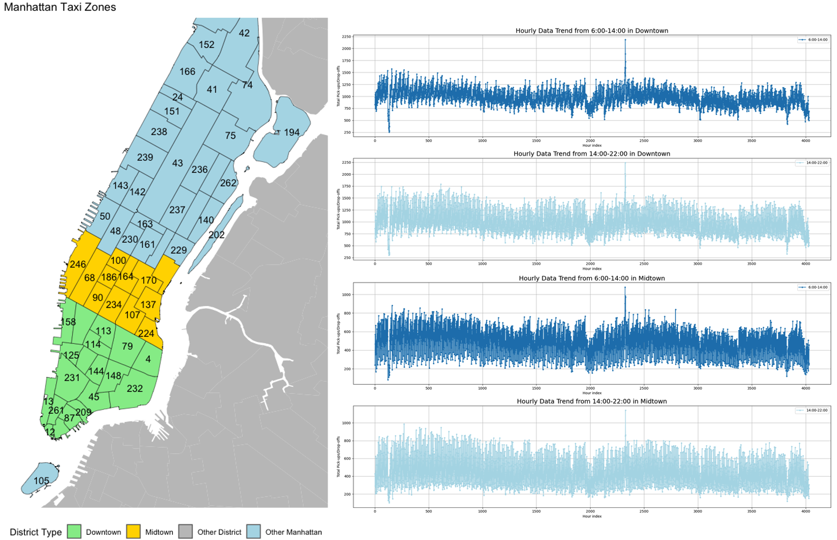
Figure S.1: Left panel: An overview of 69 districts in Manhattan. Districts colored with gold represent Midtown and districts colored with green are categorized as Downtown Manhattan. Right panel: Overall trend of the sum of pick-up and drop-off by hour in Midtown and Downtown Manhattan.

References

- Ahmed et al., (2020) Ahmed, T., Raja, H., and Bajwa, W. U. (2020). Tensor regression using low-rank and sparse tucker decompositions. SIAM Journal on Mathematics of Data Science, 2(4):944–966.
- Bai and Ng, (2002) Bai, J. and Ng, S. (2002). Determining the number of factors in approximate factor models. Econometrica, 70(1):191–221.
- Bai et al., (2018) Bai, S., Kolter, J. Z., and Koltun, V. (2018). An empirical evaluation of generic convolutional and recurrent networks for sequence modeling. arXiv preprint arXiv:1803.01271.
- Bilgin et al., (2021) Bilgin, O., Mąka, P., Vergutz, T., and Mehrkanoon, S. (2021). Tent: Tensorized encoder transformer for temperature forecasting. arXiv preprint arXiv:2106.14742.
- (5) Chen, R., Han, Y., Li, Z., Xiao, H., Yang, D., and Yu, R. (2022a). Analysis of tensor time series: tensorts. Journal of Statistical Software.
- (6) Chen, R., Yang, D., and Zhang, C.-H. (2022b). Factor models for high-dimensional tensor time series. Journal of the American Statistical Association, 117(537):94–116.
- Choi and Vishwanathan, (2014) Choi, J. H. and Vishwanathan, S. (2014). Dfacto: Distributed factorization of tensors. Advances in Neural Information Processing Systems, 27.
- De Lathauwer et al., (2000) De Lathauwer, L., De Moor, B., and Vandewalle, J. (2000). A multilinear singular value decomposition. SIAM journal on Matrix Analysis and Applications, 21(4):1253–1278.
- Fan and Gu, (2023) Fan, J. and Gu, Y. (2023). Factor augmented sparse throughput deep relu neural networks for high dimensional regression. Journal of the American Statistical Association, pages 1–15.
- Fan et al., (2017) Fan, J., Xue, L., and Yao, J. (2017). Sufficient forecasting using factor models. Journal of Econometrics, 201(2):292–306.
- Gahrooei et al., (2021) Gahrooei, M. R., Yan, H., Paynabar, K., and Shi, J. (2021). Multiple tensor-on-tensor regression: An approach for modeling processes with heterogeneous sources of data. Technometrics, 63(2):147–159.
- Guo et al., (2011) Guo, W., Kotsia, I., and Patras, I. (2011). Tensor learning for regression. IEEE Transactions on Image Processing, 21(2):816–827.
- Han et al., (2020) Han, Y., Chen, R., Yang, D., and Zhang, C.-H. (2020). Tensor factor model estimation by iterative projection. arXiv preprint arXiv:2006.02611.
- Han et al., (2022) Han, Y., Chen, R., and Zhang, C.-H. (2022). Rank determination in tensor factor model. Electronic Journal of Statistics, 16(1):1726–1803.
- Han et al., (2024) Han, Y., Yang, D., Zhang, C.-H., and Chen, R. (2024). Cp factor model for dynamic tensors. Journal of the Royal Statistical Society Series B: Statistical Methodology, page qkae036.
- Han and Zhang, (2022) Han, Y. and Zhang, C.-H. (2022). Tensor principal component analysis in high dimensional cp models. IEEE Transactions on Information Theory, 69(2):1147–1167.
- Haxby et al., (2001) Haxby, J. V., Gobbini, M. I., Furey, M. L., Ishai, A., Schouten, J. L., and Pietrini, P. (2001). Distributed and overlapping representations of faces and objects in ventral temporal cortex. Science, 293(5539):2425–2430.
- Hoff, (2015) Hoff, P. D. (2015). Multilinear tensor regression for longitudinal relational data. The Annals of Applied Statistics, 9(3):1169.
- Kilmer and Martin, (2011) Kilmer, M. E. and Martin, C. D. (2011). Factorization strategies for third-order tensors. Linear Algebra and its Applications, 435(3):641–658.
- Kossaifi et al., (2020) Kossaifi, J., Lipton, Z. C., Kolbeinsson, A., Khanna, A., Furlanello, T., and Anandkumar, A. (2020). Tensor regression networks. Journal of Machine Learning Research, 21(123):1–21.
- Lam and Yao, (2012) Lam, C. and Yao, Q. (2012). Factor modeling for high-dimensional time series: inference for the number of factors. The Annals of Statistics, 40(2):694–726.
- Li and Zhang, (2017) Li, L. and Zhang, X. (2017). Parsimonious tensor response regression. Journal of the American Statistical Association, 112(519):1131–1146.
- Li et al., (2018) Li, X., Xu, D., Zhou, H., and Li, L. (2018). Tucker tensor regression and neuroimaging analysis. Statistics in Biosciences, 10(3):520–545.
- Liu et al., (2020) Liu, Y., Liu, J., and Zhu, C. (2020). Low-rank tensor train coefficient array estimation for tensor-on-tensor regression. IEEE transactions on neural networks and learning systems, 31(12):5402–5411.
- Lock, (2018) Lock, E. F. (2018). Tensor-on-tensor regression. Journal of Computational and Graphical Statistics, 27(3):638–647.
- Luo et al., (2022) Luo, W., Xue, L., Yao, J., and Yu, X. (2022). Inverse moment methods for sufficient forecasting using high-dimensional predictors. Biometrika, 109(2):473–487.
- Luo and Zhang, (2022) Luo, Y. and Zhang, A. R. (2022). Tensor-on-tensor regression: Riemannian optimization, over-parameterization, statistical-computational gap, and their interplay. arXiv preprint arXiv:2206.08756.
- Pan and Yao, (2008) Pan, J. and Yao, Q. (2008). Modelling multiple time series via common factors. Biometrika, 95(2):365–379.
- Sen et al., (2019) Sen, R., Yu, H.-F., and Dhillon, I. S. (2019). Think globally, act locally: A deep neural network approach to high-dimensional time series forecasting. Advances in Neural Information Processing Systems, 32.
- Stock and Watson, (2002) Stock, J. H. and Watson, M. W. (2002). Forecasting using principal components from a large number of predictors. Journal of the American Statistical Association, 97(460):1167–1179.
- Sun and Li, (2017) Sun, W. W. and Li, L. (2017). Store: sparse tensor response regression and neuroimaging analysis. Journal of Machine Learning Research, 18(135):1–37.
- Tran et al., (2017) Tran, D. T., Magris, M., Kanniainen, J., Gabbouj, M., and Iosifidis, A. (2017). Tensor representation in high-frequency financial data for price change prediction. In 2017 IEEE Symposium Series on Computational Intelligence (SSCI), pages 1–7. IEEE.
- Tucker, (1966) Tucker, L. R. (1966). Some mathematical notes on three-mode factor analysis. Psychometrika, 31(3):279–311.
- Vershynin, (2010) Vershynin, R. (2010). Introduction to the non-asymptotic analysis of random matrices. arXiv preprint arXiv:1011.3027.
- Vershynin, (2018) Vershynin, R. (2018). High-dimensional probability: An introduction with applications in data science, volume 47. Cambridge university press.
- Wei et al., (2023) Wei, B., Peng, L., Guo, Y., Manatunga, A., and Stevens, J. (2023). Tensor response quantile regression with neuroimaging data. Biometrics, 79(3):1947–1958.
- Wimalawarne et al., (2016) Wimalawarne, K., Tomioka, R., and Sugiyama, M. (2016). Theoretical and experimental analyses of tensor-based regression and classification. Neural Computation, 28(4):686–715.
- Yu et al., (2022) Yu, X., Yao, J., and Xue, L. (2022). Nonparametric estimation and conformal inference of the sufficient forecasting with a diverging number of factors. Journal of Business & Economic Statistics, 40(1):342–354.
- Zhou et al., (2013) Zhou, H., Li, L., and Zhu, H. (2013). Tensor regression with applications in neuroimaging data analysis. Journal of the American Statistical Association, 108(502):540–552.