Estimating the Accuracy of the Variational Energy: Zeeman Effect in Hydrogen Atom
Abstract
For a hydrogen atom subjected to a constant magnetic field, we report the first numerical realization of the two-dimensional Non-Linearization Procedure (NLP) to estimate the accuracy of the variational energy associated with a trial function. Relevant equations of the NLP, which resemble those describing a dielectric medium with a space-dependent permittivity, are solved numerically with high accuracy using an orthogonal collocation method. As an illustration, we consider the trial function proposed in del Valle et al., Phys. Rev. A 103, (2021) 032820, and establish the accuracy of the variational energy and the local accuracy of the trial function for a strength of the magnetic field a.u. Additionally, we investigate the accuracy of the cusp parameter and quadrupole moment calculated by means of the trial function.
Introduction
Recently, the experimental measurements of ionization and transition energies of small systems have reached unprecedented high accuracy, see e.g. [1, 2, 3, 4]. In particular, measurements of ionization energies provide valuable information on stability, electronic structure, and ground state energies of ions, atoms, and molecules. When a good agreement between experimental and theoretical energies is found, it is possible to refine the value of fundamental constants, just as it was recently done for the Rydberg constant [5]. The calculation of high precision theoretical energies for small systems is usually accomplished in two steps. The first one is the calculation of a highly-accurate non-relativistic spectrum. The second one usually takes into account finite-mass (in case they were not considered in the previous step) and relativistic corrections via perturbation theory. For example, this two-step procedure was recently used to benchmark the intrashell energy transitions with in helium [6].
Most of the high-precision calculations of non-relativistic energies are rooted in the Variational Method (VM). It provides an upper bound111Also known as variational energy. to the exact ground-state energy, and also for the excited states according to the Hylleraas–Undheim–McDonald theorem [7]. The underlying ingredient behind the VM is the trial function: a parameter-dependent approximation of the unknown wave function. The presence of variational parameters allows looking for an optimal configuration to find the lowest upper bound to the ground state that the trial function can provide.
Unfortunately, the VM does not deliver information about the closeness between the upper bound and the exact ground state energy. To overcome this drawback, the formalism of lower bounds was developed in [8]. In this way, both the upper and lower bounds may define error bars of the exact theoretical energy. However, lower bounds turned out to be very crude with a rate of convergence several orders of magnitude slower than the rate of the upper bound [9]. Recent refinements of lower bounds have reached fast convergence and accuracy for some atoms such as He and Li; see [10] and [11]. However, by construction, the calculation of lower bounds is focused on trial functions that contain linear parameters only. Furthermore, this consideration does not deliver information about the accuracy of the trial function.
As an alternative to the calculation of lower bounds, we can use the connection between the VM and Perturbation Theory (PT) to estimate the accuracy of the variational energy and, most importantly, the trial function. This connection establishes that calculating the variational energy is equivalent to the computation of the first two lowest corrections in PT, see, e.g., [12, 13]. In this framework, the trial function represents the zeroth-order correction in PT of the exact wave function. Thus, as long as PT is convergent [13], the accuracy of the variational energy and the trial function can be estimated through the calculation of higher-order corrections. Consequently, the accuracy of any quantity derived from the trial function may be estimated, e.g., expectation values.
An accurate computation of corrections is a computationally expensive task using the standard formulation of PT, also known as Rayleigh-Schrödinger PT, see [14]. The main drawback of that formulation is the need of the unperturbed spectrum (at least in approximate form). Alternatively, we can use the Non-Linearization Procedure (NLP) [15]: an efficient method that only requires the unperturbed wave function of the state of interest as input. The NLP has been extensively used to estimate the accuracy of variational energies and trial functions for various systems described by a single degree of freedom, e.g., the one-dimensional quantum anharmonic oscillator [16]. Calculations performed for multidimensional systems (those described by more than one degree of freedom) have not been reported.
The present work represents the first attempt to estimate the accuracy of the variational energy and trial function via the NLP applied to a system described by more than one degree of freedom. We employ a collocation method to solve all relevant partial differential equations of the NLP. As an illustration and first step toward considering more complicated systems, we applied the formalism to a hydrogen atom in its ground state subjected to a constant magnetic field, one of the simplest atomic systems described by two degrees of freedom. We choose three relevant trial functions found in the literature proposed by Yafet et al. [17], Turbiner [18], and del Valle et al. [19]. Yafet et al. reported the first trial function in the literature. In turn, Turbiner constructed a locally accurate trial function for the first time. We also consider the compact trial function recently proposed in [19], whose construction was based on asymptotic analysis, the semi-classical expansion, and PT in powers of the strength of the magnetic field . Its high accuracy allows for investigating finite-mass effects on the energy in the range a.u. Numerical results suggested the local accuracy of the trial function; in this work, we demonstrate the correctness of such a property. In this sense, the present paper can be considered as a follow-up of [19].
This text has the following structure. We commence by describing the connection between VM and PT in section I. Then, in section II, we recapitulate the essentials of the NLP. In section III, we describe a suitable numerical realization of the NLP for the system of interest. Numerical results are reported in sections IV and V. We finish with conclusions in VI. Atomic units are used throughout this text.
I Variational Method and Perturbation Theory
The VM lies in the variational principle, which establishes
| (1) |
where is the exact ground state energy, and is a square-integrable (trial) function. The Hamiltonian operator of the system, , is assumed to be a bounded-from-below operator. The integrations are carried out over the domain on which the corresponding Schrödinger equation is defined. The upper bound is called variational energy, and is denoted as in (1). The equality between and holds if is the exact ground state eigenfunction. Let be the Hamiltonian given by
| (2) |
where denotes the Laplacian, and is the potential energy. While the Schrödinger equation
| (3) |
can be rarely solved exactly for a given , the inverse problem is always solvable: for a given square-integrable nodeless (trial) function , one can find the potential for which is the ground state wave function of the corresponding Schrödinger equation. This potential is given by
| (4) |
Then, from (1), (2), and (4), we have
where
This equation reveals that the calculation of is equivalent to computing the two-lowest order corrections in PT where represents the perturbation potential, and is the unperturbed one [12]. Thus, and play the role of the zeroth-order corrections for the energy and wave function, respectively. With higher-order corrections , we can construct
| (5) |
If the radius of convergence of the series is large enough to have inside, the partial sums of (5) may lead to highly accurate estimates of the ground state energy, see [16]. In particular, when the second-order correction is the leading one, it measures the accuracy of the variational energy [13]. Similarly, the closeness of to the exact solution can be established by calculating the corrections to the unperturbed wave function . Remarkably, a finite radius of convergence of the series (5) is obtained if is such that
| (6) |
for sufficiently large . When (6) is fulfilled, the potential is a subordinate perturbation of , see [15, 20].
II Description of the Non-Linearization Procedure
Consider the Schrödinger equation (3) defined over the domain with a Hamiltonian (2). We assume that denotes the exact and unknown ground state wave function. The function is characterized by being nodeless, i.e., it does not vanish inside . This property suggests to take the exponential representation of the function, namely
| (7) |
The phase function can be assumed to be real, is defined up to a constant222This constant only modifies the normalization of the wave function., and is non-singular. One can verify that obeys a non-linear (partial) differential equation,
| (8) |
where denotes the gradient. We consider a potential split into two components: , where is a parameter. Together with (5), the solution of (8) is taken in the form of a power series in , namely
| (9) |
The th-order corrections, and , are defined by the linear (partial) differential equation
| (10) |
where
For bound states, the requirement of zero probability current at the boundary [13].
| (11) |
must be imposed on (10). Consequently, from an integration of (10) over , we obtain the th energy correction in integral form,
| (12) |
In its one-dimensional version, Eq. (10) can always be solved, leading to written in integral form. In this case, the numerical realization of the NLP is straightforward and can be used to calculate high orders in PT, see, e.g., [16]. In contrast, numerical methods are required in the multidimensional case since the exact solution of (10) is not available. In the present work, we use a collocation method to solve (10). The choice of this method is motivated by the connection between (10) and the equation that describes a dielectric medium. To exhibit the connection, let us define three auxiliary objects:
called permittivity, electric field, and density of free charge, respectively. In terms of these, equation (10) can be expressed as
| (13) |
which is the familiar Gauss’s law describing a dielectric medium characterized by a space-dependent permittivity. Thus, calculating corrections and is equivalent to solving an electrostatic problem for each . For equations of the type (13), collocation methods have shown to be adequate tools to solve them with high accuracy; see, e.g., [21, 22].
III Zeeman Effect in Hydrogen atom
We now apply the NLP to a physically relevant atomic system described by two degrees of freedom. We consider the hydrogen atom in its ground state subjected to a constant magnetic field, giving place to the celebrated quadratic Zeeman effect.
III.1 Main Equations
The Hamiltonian operator is conveniently written in three-dimensional spherical coordinates333Therefore, in (3). ,
| (14) |
where denotes the strength of the magnetic field. We have the following assumptions behind (14): i) the infinitely-massive proton is located at the origin of coordinates, ii) the magnetic field is described by the symmetric gauge, iii) spin and other relativistic effects are neglected.
Since the ground state wave function has -dependence only, Eq. (10) takes the form
| (15) |
with444The potential is calculated through (4) using coordinates.
where . In the set of coordinates , the boundary condition (11) reads
| (16) |
Since the exact wave function is even, in the sense , so are the corrections . Consequently, we can reduce the domain from to .
III.2 Collocation Method
We assume that any correction has the representation
| (17) |
where are coefficients, and the functions and are polynomials of degree and (even) , respectively. Without loss of generality, we set as the normalization of any correction. Therefore, we demand in (17). The explicit form of the polynomials is presented further down. The exponential decay of and the polynomial growth of ensures that the boundary condition (16) is fulfilled.
Consider and as collocation points. The polynomials and are constructed in such a way that they obey
| (18) |
where denotes the Kronecker delta. After substituting the expansion (17) into (15), and demanding that the equation is satisfied at each point , it is found that a system of linear equations determines the coefficients , namely
| (19) |
where
| (20) |
and
| (21) |
We now provide the explicit form of and . The function is constructed in terms of the Laguerre polynomial of whose zeros are the collocation points. Concretely,
| (22) |
On the other hand, we use the Legendre polynomials and its zeros as collocation points to define
| (23) |
with
Functions (22) and (23) satisfy the condition (18). Furthermore, is an even function. The usage of polynomials and leads to compact expressions for the derivatives required by (20) and (21). Those expressions are found explicitly in Appendix A.
IV Results
We consider a magnetic field strength a.u. and study the accuracy provided by three different functions. All of them satisfy (6); therefore, the convergence of (5) is guaranteed.
IV.1 Yafet et al.
According to [23], Yafet et al. [17] reported the first trial function ever used to study the Zeeman effect on the hydrogen atom. The phase of this trial function has the form
| (24) |
where and are the optimal parameters at a.u. The variational energy results in
Table 1 shows the first two corrections to the variational energy for different values of , , and . The convergence in and in five significant digits has been reached with collocation points (). However, collocation points provide the correct order of magnitude of the first two corrections. From the numerical results, we observe that provides the dominant contribution to the deviation between variational energy and the exact one.
IV.2 Turbiner
The simplest function that matches the asymptotic behavior of the phase between the weak and ultra-strong regimes was proposed in [18]. The phase of this trial function reads
| (25) |
where and are optimal for the strength a.u., leading to
The value of the corrections and is presented in Table 2 for different values of , , and . Convergence in the first six decimal digits of and is achieved with collocation points. We observe that provides the dominant contribution to the deviation between variational energy and the exact one. The ratio indicates that the convergence is slow, but twice faster than the one provided by (24).
IV.3 Del Valle et al.
Based on asymptotic analysis, a semi-classical consideration, and perturbation theory, an approximation for phase was recently proposed in [19]. Defining , the trial function is written as
| (26) |
where are variational parameters. Their optimal value was already established for magnetic field strength , see [19]. In this domain, the corresponding trial function provides consistently a relative error in energy of order or less. For a.u., the optimal parameters are presented in Table 3, which lead to
| 1 | 3.23088 | 1.13922 | 0.12544 | 0.06107 | 0.04423 | 0.22745 | 0.00960 | 0.02480 |
|---|
The value of the corrections and is presented in Table 4 for different values of , , and . Note that collocation points are enough to obtain corrections with two reliable significant digits. The largest number of collocation points we used is . In this case, the value of deviates from the already converged results using fewer points (e.g., ), it suggests that collocation points are optimal for , but not for . The ratio indicates a rate of convergence at least 100 times faster compared to the rates provided by the functions (24) and (25).
| 2 | 2 | 1 | |||
|---|---|---|---|---|---|
| 5 | 5 | 1 | |||
| 10 | 10 | 1/2 | |||
| 12 | 10 | 1/3 | |||
| 15 | 15 | 1/3 | |||
| 20 | 10 | 1/4 | |||
| 30 | 15 | 1/2 | |||
| 30 | 30 | 1/2 | |||
Based on the results for shown in Table 4, we can now include uncertainty in the energy. This results in
and also in the refined value
if one considers .
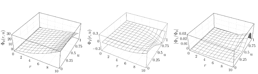
Figure 1 shows the plots of the zeroth and first-order corrections for the phase on . We can observe that the correction is small compared to , as it can be confirmed looking at the ratio also shown in Fig. 1.
Using the corrections and , we can investigate the difference between the trial function and the exact one. From (7) and (9), we construct the expansion of the exact wave function in powers of , resulting in
| (27) |
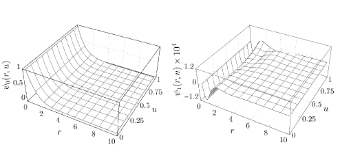
where and . The plots of and are presented in Fig. 2. According to these plots,
| (28) |
for all values of and . This fact is corroborated by the second-order correction .555According to its plot (not shown), . Thus, inequality (28) holds. As a consequence, we have verified that the trial function proposed in [19] is a locally accurate approximation of the exact ground state wave function. This feature guarantees, in particular, that all expectation values calculated via the trial function are highly accurate.
V Accuracy of Expectation Values
Let us consider the cusp parameter and the magnetic quadruple moment,
| (29) |
respectively. The presence of the magnetic field does not break the cusp condition [19]. Hence, for the exact ground state wave function. In turn, the magnetic field induces a non-zero quadrupole moment on the hydrogen atom [18].
By means of the expansion (27), we construct the series
The replacement of by in (29) defines the zeroth-order correction of and ; denoted by and , respectively. If series are convergent, higher-order corrections are used to estimate the accuracy of the zeroth-order correction , being of special interest the first-order correction .
Table 5 shows , and for the three functions considered in the previous Section, see (24), (25), and (26). Concerning the cusp parameter, Yafet’s trial function provides a vanishing . However, the first-order correction rectifies the wrong behavior of at ; thus, the corrected value improves the accuracy. On the other hand, Turbiner’s and del Valle et al. trial functions provide an accurate and the same corrected value (up to six decimal digits).
| Phase | ||||||
|---|---|---|---|---|---|---|
| Yafet et al., (24) | 0.000 000 | |||||
| Turbiner, (25) | ||||||
| Del Valle et al., (26) |
Regarding the quadrupole moment, the first-order correction does measure the deviation between the exact value and the approximated one provided by Turbiner’s and del Valle et al. trial functions, but not for Yafet’s. Only for the latter function, worsens the estimate, which indicates that higher-order corrections are needed, and that series (27) is potentially slow convergent.
VI Conclusions
For a hydrogen atom subjected to a constant magnetic field of strength a.u., we estimated the accuracy of the variational energy for three trial functions via the NLP. For all of the trial functions considered, the first-order correction of the variational energy delivered an accurate estimate of the deviation between and the exact energy. This statement was supported by the calculation of . We found that solving the relevant equations of the NLP via a collocation method requires few collocation points to achieve high accuracy in and . Furthermore, all considered trial functions lead to convergent series whose rates of convergence were estimated. Finally, we showed how the corrections coming from the NLP can be used to estimate the accuracy of any expectation value calculated by means of the trial functions. As an illustration, we considered the cusp parameter and the quadrupole moment, both defined in terms of expectation values. Additionally, we checked the local accuracy of the trial function recently proposed in [19].
The numerical implementation based on collocation methods of the NLP can serve as an efficient tool to estimate the accuracy of the variational energy when no reference value is available. In the same line, and most importantly, it can be used to estimate the accuracy of trial wave functions. Thus, the accuracy of any related quantity to bound states can be investigated (e.g., expectation values, oscillator strengths, etc.).
Studying the accuracy of trial functions describing excited states is also possible in the framework of the NLP. In this case, PT is also developed for the unperturbed nodal surface of the trial function. Then, one estimates and increases the accuracy of the approximate nodal surface using PT corrections. On the one hand, an accurate description of the nodal surface is key to some methods. For example, it is useful to circumvent the so-called fermion sign problem in the context of the fixed-node approximation in Diffusion Monte Carlo. On the other hand, nodal surfaces can also reveal unexpected symmetries, as found for the of He [25]. Based on the present results, collocation methods seem promising for studying the nodal surfaces of excited states of few-electron atomic and molecular systems with high accuracy at low computational cost.
Acknowledgments
I am grateful to A.V. Turbiner for useful discussions and essential remarks. I also thank R. Gutierrez-Jauregui and S. Cardenas-Lopez for carefully reading the text and for their valuable suggestions and comments. Financial support was provided by the (Polish) National Center for Science (NCN) under Grant No. 2019/34/E/ST1/00390 and the NSF under Grant No. PHY-2110023.
References
- Hölsch et al. [2019] N. Hölsch, M. Beyer, E. J. Salumbides, K. S. E. Eikema, W. Ubachs, C. Jungen, and F. Merkt, Phys. Rev. Lett. 122, 103002 (2019).
- Clausen et al. [2021] G. Clausen, P. Jansen, S. Scheidegger, J. A. Agner, H. Schmutz, and F. Merkt, Phys. Rev. Lett. 127, 093001 (2021).
- Markus and McCall [2019] C. R. Markus and B. J. McCall, J. Chem. Phys 150, 214303 (2019).
- Lepson et al. [2024] J. K. Lepson, P. Beiersdorfer, M. F. Gu, N. Hell, and G. V. Brown, Astrophys. J. 962, 130 (2024).
- Grinin et al. [2020] A. Grinin, A. Matveev, D. C. Yost, L. Maisenbacher, V. Wirthl, R. Pohl, T. W. Hänsch, and T. Udem, Science 370, 1061 (2020).
- Yerokhin et al. [2021] V. A. Yerokhin, V. Patkóš, and K. Pachucki, Symmetry 13 (2021).
- Hylleraas and Undheim [1930] E. A. Hylleraas and B. Undheim, Zeitschrift für Physik 65, 759 (1930).
- Temple and Chapman [1928] G. Temple and S. Chapman, Proc. R. Soc. Lond. Series A 119, 276 (1928).
- Martinazzo and Pollak [2020] R. Martinazzo and E. Pollak, Proc. Natl. Acad. Sci. U.S.A. 117, 16181 (2020).
- Nakashima and Nakatsuji [2008] H. Nakashima and H. Nakatsuji, Phys. Rev. Lett. 101, 240406 (2008).
- Ireland et al. [2022] R. T. Ireland, P. Jeszenszki, E. Mátyus, R. Martinazzo, M. Ronto, and E. Pollak, ACS Phys. Chem. Au. 2, 23 (2022).
- Epstein [2012] S. Epstein, The variation method in quantum chemistry, Physical Chemistry, a Series of Monographs (Elsevier Science, 2012).
- Turbiner [1984a] A. V. Turbiner, Sov. phys., Usp. 27, 668 (1984a).
- Schiff [1955] L. I. Schiff, Quantum mechanics (McGraw-Hill, New York, 1955).
- Turbiner [1980] A. Turbiner, Zh. Eksp. Teor. Fiz 79, 1719 (1980).
- Turbiner and del Valle [2023] A. V. Turbiner and J. C. del Valle, Quantum Anharmonic Oscillator (World Scientific, 2023).
- Yafet et al. [1956] Y. Yafet, R. Keyes, and E. Adams, J. Phys. Chem. Solids 1, 137 (1956).
- Turbiner [1984b] A. V. Turbiner, J. Phys. A 17, 859 (1984b).
- del Valle et al. [2021] J. C. del Valle, A. V. Turbiner, and A. M. Escobar-Ruiz, Phys. Rev. A 103, 032820 (2021).
- Turbiner [2010] A. V. Turbiner, Int. J. Mod. Phys. A 25, 647 (2010).
- Dang-Vu and Delcarte [1993] H. Dang-Vu and C. Delcarte, J. Comput. Phys. 104, 211 (1993).
- Chen et al. [2000] H. Chen, Y. Su, and B. D. Shizgal, J. Comput. Phys. 160, 453 (2000).
- Garstang [1977] R. H. Garstang, Rep. Prog. Phys. 40, 105 (1977).
- Baye et al. [2008] D. Baye, M. Vincke, and M. Hesse, J. Phys. B 41, 055005 (2008).
- Bressanini and Reynolds [2005] D. Bressanini and P. J. Reynolds, Phys. Rev. Lett. 95, 110201 (2005).