SVFT: Parameter-Efficient Fine-Tuning with Singular Vectors

Abstract

Popular parameter-efficient fine-tuning (PEFT) methods, such as LoRA and its variants, freeze pre-trained model weights $\mathbf{W}$ and inject learnable matrices $\mathbf{\Delta W}$. These $\mathbf{\Delta W}$ matrices are structured for efficient parameterization, often using techniques like low-rank approximations or scaling vectors. However, these methods typically show a performance gap compared to full fine-tuning. Although recent PEFT methods have narrowed this gap, they do so at the cost of additional learnable parameters. We propose SVFT, a simple approach that fundamentally differs from existing methods: the structure imposed on $\mathbf{\Delta W}$ depends on the specific weight matrix $\mathbf{W}$. Specifically, SVFT updates $\mathbf{W}$ as a sparse combination of outer products of its singular vectors, training only the coefficients (scales) of these sparse combinations. This approach allows fine-grained control over expressivity through the number of coefficients. Extensive experiments on language and vision benchmarks show that SVFT recovers up to 96% of full fine-tuning performance while training only 0.006 to 0.25% of parameters, outperforming existing methods that only recover up to 85% performance using 0.03 to 0.8% of the trainable parameter budget.

1 Introduction

Large-scale foundation models are often adapted for specific downstream tasks after pre-training. Parameter-efficient fine-tuning (PEFT) facilitates this adaptation efficiently by learning a minimal set of new parameters, thus creating an "expert" model. For instance, Large Language Models (LLMs) pre-trained on vast training corpora are fine-tuned for specialized tasks such as text summarization [12, 34], sentiment analysis [25, 20], and code completion [26] using instruction fine-tuning datasets. Although full fine-tuning (Full-FT) is a viable method to achieve this, it requires re-training and storing all model weights, making it impractical for deployment with large foundation models.

To address these challenges, PEFT techniques [13] (e.g., LoRA [14]) were introduced to significantly reduce the number of learnable parameters compared to Full-FT, though often at the cost of performance. DoRA [18] bridges this performance gap by adding more learnable parameters and being more expressive than LoRA. Almost all these methods apply a low-rank update additively to the frozen pre-trained weights, potentially limiting their expressivity. Furthermore, these adapters are agnostic to the structure and geometry of the weight matrices they modify. Finally, more expressive PEFT methods (e.g., LoRA, DoRA, BOFT [19]) still accumulate a considerable portion of learnable parameters even in their most efficient configuration (e.g., setting rank=1 in LoRA and DoRA). The storage requirements for the learnable adapters can grow very quickly when adapting to a large number of downstream tasks [16].

Is it possible to narrow the performance gap between SVFT and Full-FT while being highly parameter-efficient? We propose SVFT: Singular Vectors guided Fine-Tuning — a simple approach that involves updating an existing weight matrix by adding to it a sparse weighted combination of its own singular vectors. The structure of the induced perturbation in SVFT depends on the specific matrix being perturbed, setting it apart from all previous approaches. Our contributions can be summarized as follows:

• We introduce SVFT, a new PEFT method. Given a weight matrix ${\bm{W}}$, SVFT involves adapting it with a matrix $\Delta{\bm{W}}:=\sum_{(i,j)\in\Omega}m_{ij}{\bm{u}}_{i}{\bm{v}}_{j}^{T}$ where the $\{{\bm{u}}_{i}\}$ and $\{{\bm{v}}_{j}\}$ are the left and right singular vectors of ${\bm{W}}$, $\Omega$ is an a-priori fixed sparsity pattern, and $m_{ij}$ for $(i,j)\in\Omega$ are learnable parameters. By controlling $|\Omega|$ we can efficiently explore the accuracy vs parameters trade-off.

• SVFT achieves higher downstream accuracy, as a function of the number of trainable parameters, as compared to several popular PEFT methods (see Figure 1) and over several downstream tasks across both vision and language tasks. Our method recovers up to 96% of full fine-tuning performance while training only 0.006 to 0.25% of parameters, outperforming existing methods that only recover up to 85% performance using 0.03 to 0.8% the trainable parameter budget.

We introduce four variants for parameterizing weight updates, namely: Plain, Random, Banded, and Top-$k$ in SVFT (which differ in their choices of the fixed sparsity pattern $\Omega$) and validate these design choices empirically. Additionally, we theoretically show that for any fixed parameters budget, SVFT can induce a higher rank perturbation compared to previous PEFT techniques.

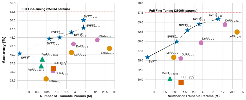
Figure 1: Performance vs total trainable parameters for GSM-8K (left) and Commonsense Reasoning (right) on Gemma-2B. $\textsc{SVFT}_{d=16}^{B/R}$ outperforms $\text{DoRA}_{r=8/16}$ with 75% less trainable parameters.

2 Related Work

Recent advancements in large language models (LLMs) have emphasized the development of PEFT techniques to enhance the adaptability and efficiency of large pre-trained language models.

LoRA. A notable contribution in this field is Low-Rank Adaptation (LoRA) [14], which freezes the weights of pre-trained models and integrates trainable low-rank matrices into each transformer layer.

For a pre-trained weight matrix ${\bm{W}}_{0}\in\mathbb{R}^{d\times n}$, LoRA constraints the weight update $\Delta{\bm{W}}$ to a low-rank decomposition: ${\bm{h}}={\bm{W}}_{0}{\bm{x}}+\Delta{\bm{W}}{\bm{x}}={\bm{W}}_{0}{\bm{x}}+\underline{{\bm{B}}{\bm{A}}}{\bm{x}}$, where ${\bm{B}}\in\mathbb{R}^{d\times r}$, ${\bm{A}}\in\mathbb{R}^{r\times n}$ and rank $r\ll\min(d,n)$. We underline the (trainable) parameters that are updated via gradient descent.

LoRA variants. We highlight some recent approaches that further improve the vanilla LoRA architecture. Vector-based Random Matrix Adaptation (VeRA) [16] minimizes the number of trainable parameters by utilizing a pair of low-rank random matrices shared between layers and learning compact scaling vectors while maintaining performance comparable to LoRA. Formally, VeRA can be expressed as: ${\bm{h}}={\bm{W}}_{0}{\bm{x}}+\Delta{\bm{W}}{\bm{x}}={\bm{W}}_{0}{\bm{x}}+\underline{\mathbf{\Lambda}_{b}}{\bm{B}}\underline{\mathbf{\Lambda}_{d}}{\bm{A}}{\bm{x}}$, where ${\bm{A}}$ and ${\bm{B}}$ are initialized randomly, frozen, and shared across layers, while $\mathbf{\Lambda}_{b}$ and $\mathbf{\Lambda}_{d}$ are trainable diagonal matrices.

An alternative approach, Weight-Decomposed Low-Rank Adaptation (DoRA) [18], decomposes pre-trained weight matrices into magnitude and direction components, and applies low-rank updates for directional updates, reducing trainable parameters and enhancing learning capacity and training stability. DoRA can be expressed as: ${\bm{h}}=\underline{{\bm{m}}}\frac{{\bm{W}}_{0}+\Delta{\bm{W}}}{\|{\bm{W}}_{0}+\Delta{\bm{W}}\|_{c}}{\bm{x}}=\underline{{\bm{m}}}\frac{{\bm{W}}_{0}+\underline{{\bm{B}}{\bm{A}}}}{\|{\bm{W}}_{0}+\underline{{\bm{B}}{\bm{A}}}\|_{c}}{\bm{x}}$, where $\|\cdot\|_{c}$ denotes the vector-wise norm of a matrix across each column. Similar to LoRA, ${\bm{W}}_{0}$ remains frozen, whereas the magnitude vector ${\bm{m}}$ (initialized to $\|{\bm{W}}_{0}\|_{c}$) and low-rank matrices ${\bm{A}},{\bm{B}}$ contain trainable parameters.

AdaLoRA [35] adaptively distributes the parameter budget across weight matrices based on their importance scores and modulates the rank of incremental matrices to manage this allocation effectively. PiSSA (Principal Singular Values and Singular Vectors Adaptation) [21] is another variant of LoRA, where matrices ${\bm{A}},{\bm{B}}$ are initialized with principal components of SVD and the remaining components are used to initialize ${\bm{W}}_{0}$. FLoRA [31] enhances LoRA by enabling each example in a mini-batch to utilize distinct low-rank weights, preserving expressive power and facilitating efficient batching, thereby extending the domain adaptation benefits of LoRA without batching limitations.

Other PEFT variants. Orthogonal Fine-tuning (OFT) [24] modifies pre-trained weight matrices through orthogonal reparameterization to preserve essential information. However, it still requires a considerable number of trainable parameters due to the high dimensionality of these matrices. Butterfly Orthogonal Fine-tuning (BOFT) [19] extends OFT’s methodology by incorporating Butterfly factorization thereby positioning OFT as a special case of BOFT. Unlike the additive low-rank weight updates utilized in LoRA, BOFT applies multiplicative orthogonal weight updates, marking a significant divergence in the approach but claims to improve parameter efficiency and fine-tuning flexibility. BOFT can be formally expressed as: ${\bm{h}}=(\underline{{\bm{R}}(m,b)}\cdot{\bm{W}}_{0}){\bm{x}}$, where the orthogonal matrix ${\bm{R}}(m,b)\in\mathbb{R}^{d\times d}$ is composed of a product of multiple orthogonal butterfly components. When $m=1$, BOFT reduces to block-diagonal OFT with block size $b$. When $m=1$ and $b=d$, BOFT reduces to the original OFT with an unconstrained full orthogonal matrix.

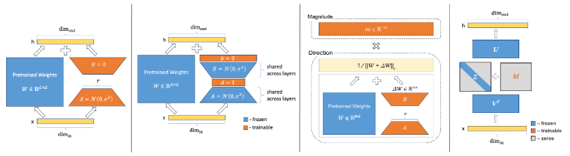
Figure 2: Schematic comparison of LoRA, VeRA, DoRA, and SVFT (left to right).

3 Method

In this section, we introduce Singular Vectors guided Fine-Tuning (SVFT). The main innovation in SVFT lies in applying structure/geometry-aware weight updates.

3.1 SVFT Formulation

We now formally describe our method, SVFT for parameter-efficient fine-tuning of a pre-trained model. Let ${\bm{W}}_{0}\in\mathbb{R}^{d_{1}\times d_{2}}$ denote a weight matrix in the pre-trained model. For instance, in a transformer block, this could be the key matrix, the query matrix, a matrix in the MLP, etc. We add a structured, learned $\Delta{\bm{W}}$ to this matrix as follows.

As a first step, we compute the Singular Value Decomposition (SVD) of the given matrix: ${\bm{W}}_{0}={\bm{U}}{\bm{\Sigma}}{\bm{V}}^{T}$. That is, ${\bm{U}}$ is the $d_{1}\times d_{1}$ matrix of left singular vectors (i.e., its columns are orthonormal), ${\bm{V}}^{T}$ is the $d_{2}\times d_{2}$ matrix of right singular vectors (i.e., its rows are orthonormal), and ${\bm{\Sigma}}$ is a $d_{1}\times d_{2}$ diagonal matrix. Then, we parameterize our weight update as $\Delta{\bm{W}}~{}=~{}{\bm{U}}{\underline{{\bm{M}}}}{\bm{V}}^{T}$, where ${\bm{U}},{\bm{V}}$ are fixed and frozen, while $\underline{{\bm{M}}}$ is a $d_{1}\times d_{2}$ sparse trainable matrix with pre-determined and fixed sparsity pattern. That is, we first pre-determine a small fixed set of elements in ${\bm{M}}$ that will be allowed to be non-zero and train only those elements. The forward pass for SVFT can be written as,

$${\bm{h}}={\bm{W}}_{0}x+\Delta{\bm{W}}x={\bm{U}}({\bm{\Sigma}}+\underline{{\bm{M}}}){\bm{V}}^{T}{\bm{x}}$$ (1)

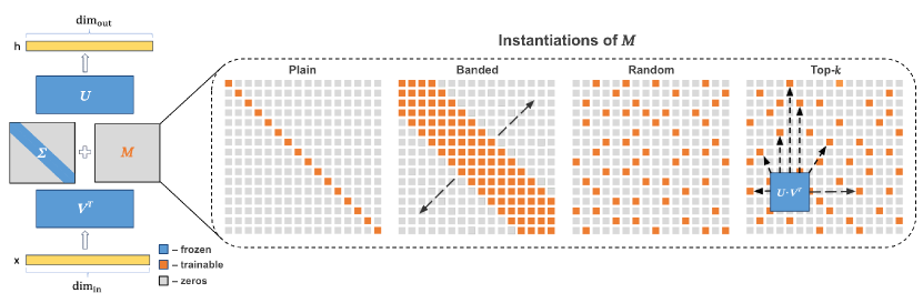
Figure 3: An Overview of SVFT. The original weights ${\bm{W}}$ are decomposed into ${\bm{U}},\mathbf{\Sigma},{\bm{V}}$. Here, ${\bm{M}}$ contains all the trainable parameters, which can be configured into patterns such as Plain, Random, Banded, and Top-$k$, represented by patterns of trainable (orange) and zero (gray) elements.

We explore four choices for $\Omega$, the a-priori fixed sparsity pattern of $\underline{{\bm{M}}}$.
Plain $\left(\textsc{SVFT}^{P}\right)$. In this variant, we constrain $\underline{{\bm{M}}}$ to be a diagonal matrix, which can be interpreted as adapting singular values and reweighting the frozen singular vectors. Since only the diagonal elements are learned, this is the most parameter-efficient SVFT variant.
Banded $\left(\textsc{SVFT}_{d}^{B}\right)$. In this approach, we populate $\underline{{\bm{M}}}$ using a banded matrix, progressively making off-diagonals learnable. Specifically, for constants $z_{1}$ and $z_{2}$, $\underline{{\bm{M}}_{ij}}=0$ if $j<i-z_{1}$ or $j>i+z_{2}$, where $z_{1},z_{2}\geq 0$. In our experiments, we set $z_{1}=z_{2}=d$ to induce off-diagonal elements that capture additional interactions beyond those represented by singular values. This banded perturbation induces local interactions, allowing specific singular values to interact with their immediate neighbors, ensuring smoother transitions. This method, although deviating from the canonical form of SVD, provides a mechanism to capture localized interactions.
Random $\left(\textsc{SVFT}_{d}^{R}\right)$. A straightforward heuristic for populating $\underline{{\bm{M}}}$ involves randomly selecting $k$ elements to be learnable.
Top-$k$ $\left(\textsc{SVFT}_{d}^{T}\right)$. The final design choice we explore involves computing the alignment between the left and right singular vectors as ${\bm{u}}_{i}^{T}{\bm{v}}_{j}$. We then select the top-$k$ elements and make them learnable. However, note that this only works when left and right singular vectors have the same size. A possible interpretation of this is we make only the top-$k$ strong interactions between singular vector directions learnable.

We illustrate these SVFT design choices in Figure 3. Our empirical results demonstrate that these simple design choices significantly enhance performance compared to state-of-the-art PEFT methods. Note that $\textsc{SVFT}^{P}$ has a fixed number of learnable parameters, while the remaining variants are configurable. We hypothesize that further innovation is likely achievable through optimizing the sparsity pattern of $\underline{{\bm{M}}}$, including efficient learned-sparsity methods. In this paper, we explore these four choices to validate the overall idea: determining a perturbation using the singular vectors of the matrix that is being perturbed.

3.2 Properties of SVFT

We highlight some properties of SVFT in the following lemma and provide insights into how its specific algebraic structure compares and contrasts with baseline PEFT methods.

Lemma: Let ${\bm{W}}_{0}$ be a matrix of size $d_{1}\times d_{2}$ with SVD given by ${\bm{U}}{\bm{\Sigma}}{\bm{V}}^{T}$. Consider an updated final matrix ${\bm{W}}_{0}+{\bm{U}}{\bm{M}}{\bm{V}}^{T}$, where ${\bm{M}}$ is a matrix of the same size as ${\bm{\Sigma}}$, which may or may not be diagonal. Then, the following holds:

1. Structure: If ${\bm{M}}$ is also diagonal (i.e. the plain SVFT), then the final matrix ${\bm{W}}_{0}+{\bm{U}}{\bm{M}}{\bm{V}}^{T}$ has ${\bm{U}}$ as its left singular vectors and $\mathrm{sign}({\bm{\Sigma}}+{\bm{M}}){\bm{V}}^{T}$ as its right singular vectors. That is, its singular vectors are unchanged, except for possible sign flips. Conversely, if ${\bm{M}}$ is not diagonal (i.e., variants of SVFT other than plain), then ${\bm{U}}$ and ${\bm{V}}$ may no longer be the singular directions of the final matrix ${\bm{W}}_{0}+{\bm{U}}{\bm{M}}{\bm{V}}^{T}$.

2. Expressivity: Given any target matrix ${\bm{P}}$ of size $d_{1}\times d_{2}$, there exists an ${\bm{M}}$ such that ${\bm{P}}={\bm{W}}_{0}+{\bm{U}}{\bm{M}}{\bm{V}}^{T}$. That is, if ${\bm{M}}$ is fully trainable, any target matrix can be realized using this method.

3. Rank: If ${\bm{M}}$ has $k$ non-zero elements, then the rank of the update ${\bm{U}}{\bm{M}}{\bm{V}}^{T}$ is at most $\min\{k,\min\{d_{1},d_{2}\}\}$. For the same number of trainable parameters, SVFT can produce a much higher rank perturbation than LoRA (eventually becoming full rank), but in a constrained structured subspace.

We provide our proofs in Appendix A. Building on this lemma, we now compare the form of the SVFT update with LoRA and VeRA.

SVFT’s $\Delta{\bm{W}}$ can be written as a sum of rank-one matrices:

$$\Delta{\bm{W}}~{}=~{}\sum_{(i,j)\in\Omega}{\underline{m_{ij}}}{\bm{u}}_{i}{\bm{v}}_{j}^{T}$$ (2)

where ${\bm{u}}_{i}$ is the $i^{th}$ left singular vector, ${\bm{v}}_{j}$ is the $j^{th}$ right singular vector, and $\Omega$ is the set of non-zero elements in ${\bm{M}}$.

Thus, our method involves adding a weighted combination of specific rank-one perturbations of the form ${\bm{u}}_{i}{\bm{v}}_{j}^{T}$.

LoRA and VeRA updates can also be expressed as sums of rank-one matrices.

$$\Delta{\bm{W}}_{\text{LoRA}}~{}=~{}\sum_{i=1}^{r}{\underline{{\bm{a}}_{i}}~{}\underline{{\bm{b}}_{i}}^{T}}\quad\text{and}\quad\Delta{\bm{W}}_{\text{VeRA}}~{}=~{}\sum_{i=1}^{r}{\underline{\alpha_{i}}}(\hat{{\bm{a}}}_{i}\odot{\underline{{\bm{\beta}}}})\hat{{\bm{b}}}_{i}^{T}$$ (3)

where $\underline{{\bm{a}}_{i}}$ and $\underline{{\bm{b}}_{j}}$ are the trainable columns of ${\bm{A}}$ and ${\bm{B}}$ matrices in LoRA. In VeRA, $\hat{{\bm{a}}}_{i}$ and $\hat{{\bm{b}}}_{i}$ are random and fixed vectors, while $\underline{{\bm{\alpha}}}$ and $\underline{{\bm{\beta}}}$ represent the diagonal elements of $\mathbf{\Lambda}_{d}$ and $\mathbf{\Lambda}_{b}$ respectively.

Note that LoRA requires $d_{1}+d_{2}$ trainable parameters per rank-one matrix, while SVFT and VeRA require only one. Although LoRA can potentially capture directions different from those achievable by the fixed $\{{\bm{u}}_{i},{\bm{v}}_{j}^{T}\}$ pairs, each of these directions incurs a significantly higher parameter cost.

VeRA captures new directions at a parameter cost similar to SVFT; however, there is a key distinction: in VeRA, each vector $\hat{{\bm{a}}}_{i}$ or $\hat{{\bm{b}}}_{i}$ appears in only one of the rank-one matrices. In contrast, in SVFT, the same vector ${\bm{u}}_{i}$ can appear in multiple terms in the summation, depending on the sparsity pattern of ${\bm{M}}$. This results in an important difference: unlike SVFT, VeRA is not universally expressive – it cannot represent any target matrix ${\bm{P}}$. Moreover, $\hat{{\bm{a}}}_{i},\hat{{\bm{b}}}_{i}$ are random, while ${\bm{u}}_{i},{\bm{v}}_{j}$ depend on ${\bm{W}}_{0}$.

Note. SVFT requires storing both left and right singular vectors due to its computation of the SVD on pre-trained weights. While this increases memory usage compared to LoRA (which is roughly double), it remains lower than BOFT. We partially address this through system-level optimizations like mixed-precision weights (e.g., bfloat16). Further exploration of memory-reduction techniques, such as quantization, is planned as future work. Importantly, inference time and memory consumption remain the same across all methods, including SVFT, as the weights can be fused.

4 Experiments

4.1 Base Models

We adapt widely-used language models, encoder-only model (DeBERTaV3_base [10]) and two decoder-only models (Gemma-2B/7B [29], LLaMA-3-8B [1]). We also experiment with vision transformer models (ViT-B/16 and ViT-L/16) [9]) pre-trained on ImageNet-21k [8], following prior work [16]. The complete details of our experimental setup and hyperparameter configurations are provided in Appendix C.
Baselines. We compare with Full Fine-Tuning (FT) updating all learnable parameters in all layers, along with LoRA [14], DoRA [18], BOFT [19] and VeRA [16].

4.2 Datasets

Language. For natural language generation (NLG) tasks, we evaluate on GSM-8K [7] and MATH [11] by fine-tuning on MetaMathQA-40K [32], following [19]. We also evaluate on 8 commonsense reasoning benchmarks (BoolQ [5], PIQA [3], SIQA [28], HellaSwag [33], Winogrande [27], ARC-easy/challenge [6], and OpenBookQA [22]). We follow the setting outlined in prior work [18, 15], where the training sets of all benchmarks are amalgamated for fine-tuning. We fine-tune on 15K examples from this training set. For natural language understanding (NLU), we evaluate on the General Language Understanding Evaluation (GLUE) benchmark consisting of classification and regression tasks, in line with [16, 14].
Vision. Our experiments on vision tasks consist of 4 benchmarks: CIFAR-100 [17], Food101 [4], RESISC45 [30], and Flowers102 [23]. We follow the setup from  [16], and fine-tune on a subset comprising 10 samples from each class.

Table 1: Performance (Accuracy) on Mathematical Reasoning (GSM-8K and MATH). #Params denote the number of trainable parameters. bold and underline represent best and second best performing PEFT method, respectively. SVFT offers superior/competitive performance at much lower #Params. For $\textsc{SVFT}^{R}_{d}$, we set $d=16$ for Gemma and $d=12$ for LLaMA-3 models.

Method	Gemma-2B			Gemma-7B			LLaMA-3-8B
	#Params	GSM-8K	MATH	#Params	GSM-8K	MATH	#Params	GSM-8K	MATH
Full-FT	2.5B	52.69	17.94	8.5B	74.67	25.70	8.0B	64.13	16.24
$\text{LoRA}_{r=32}$	26.2M	43.06	15.50	68.8M	76.57	29.34	56.6M	75.89	24.74
$\text{DoRA}_{r=16}$	13.5M	44.27	16.18	35.5M	74.52	29.84	29.1M	75.66	24.72
$\text{BOFT}^{b=8}_{m=2}$	1.22M	36.01	12.13	2.90M	71.79	28.98	4.35M	67.09	21.64
$\text{DoRA}_{r=1}$	1.19M	35.25	13.04	3.26M	74.37	26.28	2.55M	68.30	21.96
$\text{LoRA}_{r=1}$	0.82M	32.97	13.04	0.82M	72.4	26.28	1.77M	68.84	20.94
$\text{VeRA}_{r=1024}$	0.63M	36.77	14.12	0.43M	71.11	27.04	0.98M	63.76	20.28
$\textsc{SVFT}^{P}$	0.19M	40.34	14.38	0.43M	73.50	27.30	0.48M	69.22	20.44
$\textsc{SVFT}^{R}_{d}$	6.35M	50.03	15.56	19.8M	76.81	29.98	13.1M	75.90	24.22

Table 2: Evaluation results on eight commonsense reasoning benchmarks with Gemma-7B. We follow [18] for hyperparameter configurations, and report accuracy for all tasks. HS and WG denote HellaSwag [33] and WinoGrande [27], respectively. $\text{SVFT}^{P}$ offers competitive performance at a fraction of #Params. $\text{SVFT}_{d=8}^{B}$ can match $\text{LoRA}_{r=32}$ with $\sim$7x fewer parameters.

Method	#Params	BoolQ	PIQA	SIQA	HS	WG	ARC-e	ARC-c	OBQA	Average
Full-FT	8.5B	72.32	87.32	76.86	91.07	81.76	92.46	82.76	89.00	84.19
$\text{LoRA}_{r=32}$	68.8M	71.55	87.95	77.27	91.80	79.71	92.67	82.16	86.40	83.69
$\text{DoRA}_{r=16}$	35.5M	71.46	87.59	76.35	92.11	78.29	92.00	80.63	85.60	83.00
$\text{DoRA}_{r=1}$	3.31M	68.22	86.72	75.23	91.14	78.13	91.87	83.19	86.20	82.59
$\text{VeRA}_{r=2048}$	1.49M	64.25	86.28	74.04	86.96	69.00	92.76	82.33	82.00	79.70
$\text{LoRA}_{r=1}$	0.82M	65.44	86.28	75.02	89.91	75.92	91.79	81.91	85.40	81.46
$\textsc{SVFT}^{P}$	0.51M	67.92	86.45	75.47	86.92	74.03	91.80	81.23	83.00	80.85
$\textsc{SVFT}^{B}_{d=8}$	9.80M	71.90	86.98	76.28	91.55	78.76	92.80	83.11	85.40	83.35

Table 3: DeBERTaV3_base with different adaptation methods on the GLUE benchmark. We report matched accuracy for MNLI, Matthew’s correlation for CoLA, Pearson correlation for STS-B, and accuracy for other tasks. Higher is better for all tasks. * indicates numbers published in prior work.

Method	#Params	MNLI	SST-2	MRPC	CoLA	QNLI	QQP	RTE	STS-B	Avg.
Full-FT*	184M	89.90	95.63	89.46	69.19	94.03	92.40	83.75	91.60	88.25
$\text{LoRA*}_{r=8}$	1.33M	90.65	94.95	89.95	69.82	93.87	91.99	85.20	91.60	88.50
$\text{DoRA}_{r=4}$	0.75M	89.92	95.41	89.10	69.37	94.14	91.53	87.00	91.80	88.53
$\text{BOFT*}^{b=8}_{m=2}$	0.75M	90.25	96.44	92.40	72.95	94.23	92.10	88.81	91.92	89.89
$\text{LoRA}_{r=1}$	0.17M	90.12	95.64	86.43	69.13	94.18	91.43	87.36	91.52	88.23
$\text{VeRA}_{r=1024}$	0.09M	89.93	95.53	87.94	69.06	93.24	90.4	87.00	88.71	87.73
$\textsc{SVFT}^{P}$	0.06M	89.69	95.41	88.77	70.95	94.27	90.16	87.24	91.80	88.54
SVFT${}^{R}_{d=2}$	0.28M	89.97	95.99	88.99	72.61	93.90	91.50	88.09	91.73	89.10

Table 4: Performance on image classification benchmarks. For LoRA, DoRA and $\textsc{SVFT}^{B}$, we adapt {Q, K, V, U, D} modules of the transformer. For $\textsc{SVFT}^{P}$, we adapt only {Q, V} to keep it comparable with VeRA. We report accuracy for all tasks.

Method	ViT-B			ViT-L
	#Params	CIFAR100	Flowers102	#Params	Food101	Resisc45
Head	-	78.25	98.42	-	75.57	64.10
Full-FT	85.8M	85.35	98.37	303.3M	77.83	76.83
$\text{LoRA}_{r=8}$	1.32M	84.10	99.23	3.54M	77.13	79.62
$\text{DoRA}_{r=8}$	1.41M	85.03	99.30	3.76M	76.41	78.32
$\text{BOFT}^{b=4}_{m=4}$	0.11M	85.54	98.59	2.95M	78.42	74.70
$\text{LoRA}_{r=1}$	0.16M	84.86	96.88	0.44M	75.97	78.02
$\text{DoRA}_{r=1}$	0.25M	84.46	99.15	0.66M	75.90	78.02
$\text{VeRA}_{r=256}$	24.6K	83.38	98.59	0.06M	75.97	72.44
$\textsc{SVFT}^{P}$	18.5K	83.85	98.93	0.05M	75.95	71.97
$\textsc{SVFT}^{B}_{d=2}$	0.27M	84.72	99.28	0.74M	77.94	79.70
$\textsc{SVFT}^{B}_{d=8}$	0.93M	85.69	98.88	2.5M	78.36	73.83

5 Results

5.1 Performance on Language Tasks

Natural Language Generation.

We present results on mathematical question answering against baseline PEFT techniques across three base models – varying from 2B to 8B parameters in Table 1. To ensure a comprehensive comparison, we test baseline techniques (LoRA, DoRA) with different configurations, and varying hyper-parameters like rank to cover a range of learnable parameters from low to high. Note that even when the rank is as low as 1, both methods yield more trainable parameters than $\textsc{SVFT}^{P}$. $\textsc{SVFT}^{P}$ ($\sim$0.2M) shows as much as $18\%$ relative improvement over techniques that use 6$\times$ more trainable parameters ($\text{BOFT}^{b=8}_{m=2}$, $\text{LoRA}_{r=1}$). Against techniques of comparable sizes (VeRA), $\textsc{SVFT}^{P}$ achieves 15.5% relative improvement on average. Even in the default regime, $\textsc{SVFT}^{R}_{d}$ matches techniques with at least $3\times$ more trainable parameters. Notably, on GSM-8K, $\textsc{SVFT}^{R}_{d}$ again achieves 96% of the full fine-tuning performance, while $\text{DoRA}_{r=16}$ recovers 86% with $2\times$ more parameters than $\textsc{SVFT}^{R}_{d}$.

Commonsense Reasoning.

In Table 2, we compare performance on commonsense reasoning benchmarks with Gemma-7B, and observe similar trends. In the lower and moderately parameterized regime ($\sim$0.43M), $\textsc{SVFT}^{P}$ shows competitive performance in comparison to $\textsc{LoRA}_{r=1}$ and $\text{DoRA}_{r=1}$, which have 1.9$\times$ and 7.7$\times$ more parameters, respectively. Against VeRA, which trains 3.5$\times$ more parameters, $\textsc{SVFT}^{P}$ shows a relative improvement of $\sim$1.16%. Similarly, $\textsc{SVFT}^{B}_{d=8}$ also matches or exceeds methods that use up to 7$\times$ more trainable parameters. For instance, $\textsc{SVFT}^{B}_{d=8}$ attains an average performance of 83.35% with only 9.8M parameters, closely matching $\text{LoRA}_{r=16}$ (83.69%, 68.8M parameters). We observe similar trends with Gemma-2B (refer Table 8).

Natural Language Understanding.

Results on the GLUE benchmark are summarized in Table 3. SVFT matches $\text{LoRA}_{r=8}$ and $\text{DoRA}_{r=4}$ which use 12-22$\times$ more trainable parameters. Similarly, when compared to OFT and BOFT, $\textsc{SVFT}^{P}$ maintains a comparable average performance despite being 12$\times$ smaller. These results highlight SVFT’s ability to strike a balance between parameter efficiency and performance, making it an attractive PEFT choice for simple classification tasks.

Parameter efficiency. In Figure 1, we plot the performance of SVFT on mathematical reasoning and commonsense reasoning against other PEFT techniques across a range of configurations. Across trainable parameter budgets ranging from lowest to highest, SVFT obtains the best overall performance, matching methods that require significantly more trainable parameters. These results establish SVFT as a Pareto-dominant approach for parameter-efficient fine-tuning.

5.2 Performance on Vision Tasks

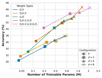
Figure 4: Performance variation with $\textsc{SVFT}^{B}_{d}$ based on the adapted weight matrices – GSM-8K with Gemma-2B. Adapting more target weight types results in greater gains in performance. Interestingly, for a fixed parameter budget, adapting ${\bm{U}}$ and ${\bm{D}}$ weight types gives greater lifts than adapting ${\bm{Q}}$ and ${\bm{V}}$.

Table 4 contrasts SVFT against other PEFT techniques on image classification benchmarks using ViT-B and ViT-L models. For ViT-B, $\textsc{SVFT}^{B}_{d=8}$ surpasses full fine-tuning performance along with $\text{LoRA}_{r=8}$ and $\text{DoRA}_{r=8}$ on CIFAR-100. $\textsc{SVFT}^{B}_{d=2}$ matches $\text{LoRA}_{r=8}$ and $\text{DoRA}_{r=8}$ on Flowers102 with up to $5\times$ fewer parameters. For ViT-L, $\textsc{SVFT}^{B}_{d}$ also demonstrates superior or competitive performance on both Food101 and Resisc45, with significantly lower trainable parameters compared to both fully fine-tuned models and other state-of-the-art PEFT approaches.

5.3 Contribution of Each Weight Type

In Figure 4, we investigate the contribution of each weight type. Starting with the base configuration, we apply $\textsc{SVFT}^{B}_{d}$ to the ${\bm{Q}}$ and ${\bm{V}}$ weights in each transformer block and report the performance. We then incrementally add the remaining weight modules (${\bm{K}},{\bm{U}},{\bm{D}},{\bm{O}},{\bm{G}}$) and observe the changes in performance. For each configuration, we also vary the trainable parameters by incrementing the total learnable off-diagonals.

Note that applying $\textsc{SVFT}^{B}_{d}$ to ${\bm{U}},{\bm{D}},{\bm{O}},$ and ${\bm{G}}$ does not increase trainable parameters as much as applying LoRA/DoRA to these modules (Table 7). For example, for a large matrix of shape $d_{1}\times d_{2}$, $\text{LoRA}_{r=1}$ learns $d_{1}+d_{2}$ parameters, while $\textsc{SVFT}^{P}$ learns $\min(d_{1},d_{2})$ parameters. We observe that adapting only ${\bm{U}}$ and ${\bm{D}}$ with SVFT yields up to a $10\%$ relative improvement over adapting ${\bm{Q}}$ and ${\bm{V}}$ for the same parameter budget ($\sim 0.8M$). Our findings indicate that adapting more weight types enhances performance.

Table 5: Results on fine-tuning Gemma-2B with SVFT using different ${\bm{M}}$ parameterizations.

Structure	#Params	GSM-8K	MATH
Plain	0.2M	40.34	14.38
Banded	3.3M	46.47	16.04
	6.4M	47.84	15.68
Random	3.3M	47.76	15.98
	6.4M	50.03	15.56
Top-$k$	3.3M	48.00	15.80
	6.4M	49.65	15.32

Table 6: Impact of pre-trained weight quality. Results on GSM-8K after fine-tuning on Pythia-2.8B checkpoints at different stages of pre-training (PT). Compared to LoRA, SVFT benefits more from better pre-trained weights. SVFT outperforms LoRA in both cases.

Method	#Params	PT Steps		$\Delta$Perf
		39K	143K
Full-FT	2.5B	21.00	30.09	9.09
LoRA	5.24M	11.22	18.95	7.73
SVFT	5.56M	15.08	23.19	8.11

5.4 Impact of ${M}$’s Structure on Performance

We analyze the impact of different parameterizations of ${\bm{M}}$ (Plain, Banded, Random, Top-$k$) on downstream performance. To ensure a fair comparison, we match the number of trainable coefficients across all variants. As shown in Table 6, both Random and Top-$k$ variants outperform Banded on the GSM-8K dataset. However, this improvement comes at the cost of performance on MATH. This observation suggests that the choice of parameterization has a significant impact on model performance, and the effectiveness of a particular structure may vary depending on the downstream task.

5.5 Impact of Pre-trained Weight Quality

A key feature of SVFT is that the weight update depends on the pre-trained weights ${\bm{W}}$. We therefore ask the following question: Does the quality of pre-trained weights have a disproportionate impact on SVFT? To answer this, we consider two checkpoints from the Pythia suite [2] at different stages of training, i.e., 39K steps and 143K steps, respectively. We fine-tune each of these checkpoints independently with Full-FT, LoRA, and SVFT. We then compare the increase in performance ($\Delta$Perf). As shown in Table 6, compared to LoRA, SVFT benefits more from better pre-trained weights. We also note that SVFT outperforms LoRA in both settings, suggesting that the benefits of inducing a $\Delta{\bm{W}}$ that explicitly depends on ${\bm{W}}$ are beneficial even when ${\bm{W}}$ is sub-optimal.

6 Discussion

Limitations. Despite significantly reducing learnable parameters and boosting performance, SVFT incurs some additional GPU memory usage. Unlike LoRA and its variants, SVFT necessitates computing the SVD and storing both left and right singular vectors. While memory consumption remains lower than BOFT, it’s roughly double that of LoRA. We mitigate this in our work by employing system-level optimizations like mixed-precision weights (e.g., bfloat16). However, similar to the scaling explored in [31], memory usage should amortize with the increasing scale of adaptation tasks. In future work we will explore quantization and other techniques to address memory concerns.

Broader Impact. Our work enables easier personalization of foundational models, which can have both positive and negative societal impacts. Since our method provides computational efficiency (smaller parameter footprint), it will be less expensive to enable personalization.

7 Conclusion

This work introduces SVFT, a novel and efficient PEFT approach that leverages the structure of pre-trained weights to determine weight update perturbations. We propose four simple yet effective sparse parameterization patterns, offering flexibility in controlling the model’s expressivity and the number of learnable parameters. Extensive experiments on language and vision tasks demonstrate SVFT’s effectiveness as a PEFT method across diverse parameter budgets. Furthermore, we theoretically show that SVFT can induce higher-rank perturbation updates compared to existing methods, for a fixed parameter budget. In future work, we aim to develop principled methods to generate sparsity patterns, potentially leading to further performance improvements.

Appendix

The appendix is organized as follows.

• In  Appendix A, we give proofs for the lemmas outlined in  3.2.

• In  Appendix B, we compare how the trainable parameters count for different PEFT techniques (LoRA, DoRA, VeRA) versus our method SVFT.

• In  Appendix C, we describe results for additional experiments and provide implementation details for all the experiments.

Appendix A Proofs

We provide brief proofs for the Structure, Expressivity and the Rank lemmas for SVFT:

1. Structure: If ${\bm{M}}$ is diagonal, then the final matrix ${\bm{W}}_{0}+U{\bm{M}}V^{T}$ can be written as
   $U(\Sigma+{\bm{M}})V^{T}$ since ${\bm{W}}_{0}=U\Sigma V^{T}$, where $(\Sigma+{\bm{M}})$ is also a diagonal matrix. Thus, $U(\Sigma+{\bm{M}})V^{T}$ is a valid and unique SVD of ${\bm{W}}_{0}+U{\bm{M}}V^{T}$ up to sign flips in the singular vectors.

2. Expressivity: Finding ${\bm{M}}$ for any target matrix $P$ of size $d_{1}\times d_{2}$ such that $P={\bm{W}}_{0}+U{\bm{M}}V^{T}$ is the same as finding ${\bm{M}}$ for a new target matrix $P^{\prime}=P-{\bm{W}}_{0}$ such that $P^{\prime}=U{\bm{M}}V^{T}$. For a full SVD, the dimension of ${\bm{M}}$ is $d_{1}\times d_{2}$ and since the dimension of $P^{\prime}$ is also $d_{1}\times d_{2}$, $P^{\prime}=U{\bm{M}}V^{T}$ is a bijection and ${\bm{M}}=U^{T}(P-{\bm{W}}_{0})V$ (since $U$ and $V$ are orthogonal).

3. Rank: If ${\bm{M}}$ has $k$ non-zero elements, then the rank of the update $U{\bm{M}}V^{T}$ will be upper bounded by $k$ (since by Gaussian elimination, $k$ or less elements will remain, the best case being all $k$ elements in the diagonal). We also know that the rank is upper bounded by $\min\{d_{1},d_{2}\}$, giving an achievable upper bound on the rank as $\min\{k,\min\{d_{1},d_{2}\}\}$.

Appendix B Parameter Count Analysis

Table 7: Parameter count analysis. $L_{\text{tuned}}$, $D_{\text{model}}$, $r$, $k$ denote total layers being adapted, hidden dimension, rank, and additional off-diagonals respectively.

Method	Trainable Parameter Count
LoRA	$2\times L_{\text{tuned}}\times D_{\text{model}}\times r$
DoRA	$L_{\text{tuned}}\times D_{\text{model}}\times(2r+1)$
VeRA	$L_{\text{tuned}}\times(D_{\text{model}}+r)$
$\text{SVFT}^{P}$	$L_{\text{tuned}}\times D_{\text{model}}$
$\text{SVFT}^{B}_{d=k}$	$L_{\text{tuned}}\times(D_{\text{model}}\times k+(D_{\text{model}}-k)(k+1))$

Appendix C Additional Experiments and Implementation Details

All of our experiments are conducted on a Linux machine (Debian GNU) with the following specifications: 2xA100 80 GB, Intel Xeon CPU @ 2.20GHz with 12 cores, and 192 GB RAM. For all our experiments (including baseline experiments), we utilize hardware-level optimizations like mixed weight precision (e.g., bfloat16) whenever possible.

C.1 Commonsense Reasoning Gemma-2B

We evaluate and compare SVFT variants against baseline PEFT methods on commonsense reasoning tasks with Gemma-2B model and tabulate results in Table 8.

Table 8: Results with Gemma-2B on eight commonsense reasoning benchmarks. We follow [18] for hyperparameter configurations, and report accuracy for all tasks.

Method	#Params	BOOLQ	PIQA	SIQA	HellaSwag	Winogrande	ARC-E	ARC-C	OBQA	Average
Full-FT	2.5B	63.57	74.1	65.86	70.00	61.95	75.36	59.72	69	67.45
$\text{LoRA}_{r=32}$	26.2M	63.11	73.44	63.20	47.79	52.95	74.78	57.16	67.00	62.43
$\text{LoRA}_{r=16}$	13.5M	62.87	73.93	65.34	53.16	55.51	76.43	59.55	68.4	64.40
$\text{BOFT}_{m=2}^{b=8}$	1.22M	59.23	63.65	47.90	29.93	50.35	59.04	42.66	41.00	49.22
$\text{VeRA}_{r=2048}$	0.66M	62.11	64.31	49.18	32.00	50.74	58.08	42.83	42.6	50.23
$\text{LoRA}_{r=1}$	0.82M	62.2	69.31	56.24	32.47	51.53	69.52	48.8	56.4	55.81
$\text{DoRA}_{r=1}$	1.19M	62.17	68.77	55.93	32.95	51.22	68.81	48.72	55.6	55.52
$\textsc{SVFT}^{P}$	0.19M	62.26	70.18	56.7	32.47	47.04	69.31	50.08	58.4	55.81
$\textsc{SVFT}^{B}_{d=16}$	6.35M	63.42	73.72	63.86	71.21	59.58	73.69	54.77	66.6	65.86

C.2 Additional Vision Experiments

For vision tasks, we compare the SVFT banded variants and SVFT plain with baseline PEFT methods on classification vision tasks using ViT-Base and ViT-Large models in  Table 9.

Table 9: Performance on image classification benchmarks. For LoRA, DoRA and $\textsc{SVFT}^{B}_{d}$, we adapt {Q, K, V, U, D} modules of the transformer. For $\textsc{SVFT}^{P}$, we adapt only {Q, V} to keep it comparable with VeRA. We report accuracy for all tasks.

Method	ViT-B					ViT-L
	#Params	CIFAR100	Flowers102	Food101	Resisc45	#Params	CIFAR100	Flowers102	Food101	Resisc45
Head	-	78.25	98.42	74.93	59.95	-	82.95	98.75	75.57	64.10
Full-FT	85.8M	85.35	98.37	76.32	68.03	303.3M	86.56	97.87	77.83	76.83
$\text{LoRA}_{r=8}$	1.32M	84.41	99.23	76.02	76.86	0.35M	86.00	97.93	77.13	79.62
$\text{DoRA}_{r=8}$	1.41M	85.03	99.30	75.88	76.95	3.76M	83.55	98.00	76.41	78.32
$\text{BOFT}^{b=2}_{m=2}$	0.07M	85.55	98.54	76.06	67.70	0.20M	87.84	97.95	77.90	73.97
$\text{BOFT}^{b=4}_{m=4}$	0.11M	85.54	98.59	76.51	69.44	0.30M	87.72	97.95	78.42	74.70
$\text{LoRA}_{r=1}$	0.16M	84.86	96.88	73.35	76.33	0.44M	85.97	98.28	75.97	78.02
$\text{DoRA}_{r=1}$	0.25M	84.46	99.15	74.80	77.06	0.66M	84.06	98.11	75.90	78.02
VeRA	24.6K	83.38	98.59	75.99	70.43	61.4K	86.77	98.94	75.97	72.44
$\textsc{SVFT}^{P}$	18.5K	83.85	98.93	75.68	67.19	49.2K	86.74	97.56	75.95	71.97
$\textsc{SVFT}^{B}_{d=2}$	0.28M	84.72	99.28	75.64	72.49	0.74M	86.59	98.24	77.94	79.70
$\textsc{SVFT}^{B}_{d=4}$	0.50M	83.17	98.52	76.54	66.65	1.32M	87.10	97.71	76.67	71.10
$\textsc{SVFT}^{B}_{d=8}$	0.94M	85.69	98.88	76.70	70.41	2.50M	87.26	97.89	78.36	73.83

C.3 Are All Singular Vectors Important?

To determine the importance of considering all singular vectors and singular values during fine-tuning, we reduce the rank of ${\bm{U}}$ and ${\bm{V}}$, and truncate ${\bm{\Sigma}}$ and ${\bm{M}}$ to an effective rank of $r$. If the original weight matrix ${\bm{W}}\in\mathbb{R}^{m\times n}$, then after truncation, ${\bm{U}}\in\mathbb{R}^{m\times r},{\bm{V}}\in\mathbb{R}^{n\times r}$. This truncation significantly reduces the number of trainable parameters, so we compensate by increasing the number of off-diagonal coefficients ($d$) in ${\bm{M}}$.

Our results, with four different configurations of $r$ and $d$, are presented in Table 10. The findings show that a very low rank ($r=128$) leads to poor performance, even when parameters are matched. A reasonably high rank of $r=1536$, which is 75% of the full rank, still fails to match the performance of the full-rank variant that has 0.25$\times$ the trainable parameters. This indicates that all singular vectors significantly contribute to the end task performance when fine-tuning with SVFT, and that important information is lost even when truncating sparingly.

Table 10: Performance with varying rank ($r$) and the off-diagonal elements ($d$) of ${\bm{M}}$. When $r=2048$, the update is full-rank.

Rank ($r$)	Diags ($d$)	#Params	GSM-8K	MATH
128	64	1.55M	0.98	0.21
1536	-	0.15M	16.37	3.64
1536	2	0.74M	25.01	6.04
2048	-	0.19M	40.34	14.38

C.4 Performance vs Total Trainable Parameters

In addition to the experiments performed in Figure 1 for Gemma-2B on challenging natural language generation (NLG) tasks like GSM-8K and Commonsense Reasoning, we also plot the performance vs total trainable parameters for larger state-of-the-art models like Gemma-7B and LLaMA-3-8B on GSM-8K. Figure 5 further demonstrates SVFT’s Pereto-dominance. On larger models, we observe that full-finetuning overfits, leading to sub-optimal performance in comparison to PEFT methods.

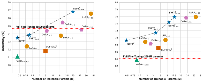
Figure 5: Performance versus total trainable parameters for GSM-8K on Gemma-7B (left) and LLaMA-3-8B (right).

C.5 Settings for Language Tasks

Natural Language Understanding.

We fine-tune the DeBERTaV3_base [10] model and apply SVFT to all linear layers in every transformer block of the model. We only moderately tune the batch size, learning rate, and number of training epochs. We use the same model sequence lengths used by  [19] to keep our comparisons fair. The hyperparameters used in our experiments can be found in  Table 11.

Table 11: Hyperparameter setup used for DeBERTaV3_base on the GLUE benchmark.

Method	Dataset	MNLI	SST-2	MRPC	CoLA	QNLI	QQP	RTE	STS-B
	Optimizer	AdamW
	Warmup Ratio	0.1
	LR Schedule	Linear
	Learning Rate (Head)	6E-03
	Max Seq. Len.	256	128	320	64	512	320	320	128
	# Epochs	10	10	30	20	10	6	15	15
SVFTP	Batch Size	32	32	16	16	32	16	4	32
	Learning Rate	5E-02	5E-02	5E-02	8E-02	8E-02	5E-02	5E-02	5E-02
SVFT${}^{R}_{d=2}$	Batch Size	32	32	16	16	32	32	16	32
	Learning Rate	1E-02	1E-02	1E-02	1E-02	3E-02	1E-02	3E-02	1E-02

Natural Language Generation.

See the hyperparameters used in our experiments in  Table 12. For LoRA, DoRA, we adapt $Q,K,V,U,D$ matrices. We apply BOFT on $Q,V$ matrices since applying on multiple modules is computationally expensive. For VeRA, which enforces a constraint of uniform internal dimensions for shared matrices, we apply on $G,U$ projection matrices as it yields the highest number of learnable parameters. We apply SVFT on $Q,K,V,U,D,O,G$ for the Gemma family of models, and $U,D,O,G$ for LLaMA-3-8B. Note that applying SVFT on these modules does not increase trainable parameters at the same rate as applying LoRA or DoRA on them would. We adopt the code base from https://github.com/meta-math/MetaMath.git for training scripts and evaluation setups and use the fine-tuning data available at https://huggingface.co/datasets/meta-math/MetaMathQA-40K.

Table 12: Hyperparameter setup used for fine-tuning on MetaMathQA-40K.

Hyperparameter	Gemma-2B		Gemma-7B		LLaMA-3-8B
	SVFTP	SVFT${}^{R}_{d=16}$	SVFTP	SVFT${}^{R}_{d=16}$	SVFTP	SVFT${}^{R}_{d=12}$
Optimizer	AdamW
Warmup Ratio	0.1
LR Schedule	Cosine
Learning Rate	5E-02	1E-03	5E-02	1E-03	5E-02	1E-03
Max Seq. Len.	512
# Epochs	2
Batch Size	64

Commonsense Reasoning.

See the hyperparameters used in our experiments in  Table 13. We adopt the same set of matrices as that of natural language generation tasks. We use the code base from https://github.com/AGI-Edgerunners/LLM-Adapters, which also contains the training and evaluation data.

Table 13: Hyperparameter setup used for fine-tuning on commonsense-15K.

Hyperparameter	Gemma-2B		Gemma-7B
	SVFTP	SVFT${}^{B}_{d=8}$	SVFTP	SVFT${}^{B}_{d=8}$
Optimizer	AdamW
Warmup Steps	100
LR Schedule	Linear
Max Seq. Len.	512
# Epochs	3
Batch Size	64
Learning Rate	5E-02	5E-03	5E-02	1E-03

C.6 Settings for Vision Tasks

Table 14: Hyperparameter setup used for fine-tuning on all vision tasks.

Hyperparameter	ViT-B	ViT-L
Optimizer	AdamW
Warmup Ratio	0.1
Weight Decay	0.01
LR Schedule	Linear
# Epochs	10
Batch Size	64
$\textsc{SVFT}^{P}$ Learning Rate (Head)	4E-03
$\textsc{SVFT}^{P}$ Learning Rate	5E-02
$\textsc{SVFT}^{B}_{d=2}$ Learning Rate (Head)	4E-03
$\textsc{SVFT}^{B}_{d=2}$ Learning Rate	5E-02
$\textsc{SVFT}^{B}_{d=8}$ Learning Rate (Head)	4E-03
$\textsc{SVFT}^{B}_{d=8}$ Learning Rate	5E-03

For each dataset in the vision tasks, we train on 10 samples per class, using 2 examples per class for validation, and test on the full test set. Similar to previous literature, we always train the classifier head for these methods since the number of classes is large. The parameter counts do not include the number of parameters in the classification head. The hyperparameters are mentioned in  Table 14. We tune the learning rates for SVFT and BOFT select learning rates for other methods from [16], run training for 10 epochs, and report test accuracy for the best validation model. For all methods, since classification head has to be fully trained, we report the parameter count other than the classification head.

References

- [1] Meta AI. Introducing meta llama 3: The most capable openly available llm to date. April 2024.
- [2] Stella Biderman, Hailey Schoelkopf, Quentin Anthony, Herbie Bradley, Kyle O’Brien, Eric Hallahan, Mohammad Aflah Khan, Shivanshu Purohit, USVSN Sai Prashanth, Edward Raff, Aviya Skowron, Lintang Sutawika, and Oskar van der Wal. Pythia: A suite for analyzing large language models across training and scaling, 2023.
- [3] Yonatan Bisk, Rowan Zellers, Ronan Le Bras, Jianfeng Gao, and Yejin Choi. Piqa: Reasoning about physical commonsense in natural language. In Thirty-Fourth AAAI Conference on Artificial Intelligence, 2020.
- [4] Lukas Bossard, Matthieu Guillaumin, and Luc Van Gool. Food-101 – mining discriminative components with random forests. In European Conference on Computer Vision, 2014.
- [5] Christopher Clark, Kenton Lee, Ming-Wei Chang, Tom Kwiatkowski, Michael Collins, and Kristina Toutanova. Boolq: Exploring the surprising difficulty of natural yes/no questions, 2019.
- [6] Peter Clark, Isaac Cowhey, Oren Etzioni, Tushar Khot, Ashish Sabharwal, Carissa Schoenick, and Oyvind Tafjord. Think you have solved question answering? try arc, the ai2 reasoning challenge, 2018.
- [7] Karl Cobbe, Vineet Kosaraju, Mohammad Bavarian, Mark Chen, Heewoo Jun, Lukasz Kaiser, Matthias Plappert, Jerry Tworek, Jacob Hilton, Reiichiro Nakano, Christopher Hesse, and John Schulman. Training verifiers to solve math word problems. arXiv preprint arXiv:2110.14168, 2021.
- [8] Jia Deng, Wei Dong, Richard Socher, Li-Jia Li, Kai Li, and Li Fei-Fei. Imagenet: A large-scale hierarchical image database. In 2009 IEEE conference on computer vision and pattern recognition, pages 248–255. Ieee, 2009.
- [9] Alexey Dosovitskiy, Lucas Beyer, Alexander Kolesnikov, Dirk Weissenborn, Xiaohua Zhai, Thomas Unterthiner, Mostafa Dehghani, Matthias Minderer, Georg Heigold, Sylvain Gelly, Jakob Uszkoreit, and Neil Houlsby. An image is worth 16x16 words: Transformers for image recognition at scale. In International Conference on Learning Representations, 2021.
- [10] Pengcheng He, Jianfeng Gao, and Weizhu Chen. Debertav3: Improving deberta using electra-style pre-training with gradient-disentangled embedding sharing, 2023.
- [11] Dan Hendrycks, Collin Burns, Saurav Kadavath, Akul Arora, Steven Basart, Eric Tang, Dawn Song, and Jacob Steinhardt. Measuring mathematical problem solving with the math dataset, 2021.
- [12] Karl Moritz Hermann, Tomáš Kočiský, Edward Grefenstette, Lasse Espeholt, Will Kay, Mustafa Suleyman, and Phil Blunsom. Teaching machines to read and comprehend. In Proceedings of the 28th International Conference on Neural Information Processing Systems, NIPS’15, page 1693–1701. MIT Press, 2015.
- [13] Neil Houlsby, Andrei Giurgiu, Stanislaw Jastrzebski, Bruna Morrone, Quentin De Laroussilhe, Andrea Gesmundo, Mona Attariyan, and Sylvain Gelly. Parameter-efficient transfer learning for NLP. In Proceedings of the 36th International Conference on Machine Learning, Proceedings of Machine Learning Research. PMLR, 2019.
- [14] Edward J Hu, Yelong Shen, Phillip Wallis, Zeyuan Allen-Zhu, Yuanzhi Li, Shean Wang, Lu Wang, and Weizhu Chen. LoRA: Low-rank adaptation of large language models. In International Conference on Learning Representations, 2022.
- [15] Zhiqiang Hu, Lei Wang, Yihuai Lan, Wanyu Xu, Ee-Peng Lim, Lidong Bing, Xing Xu, Soujanya Poria, and Roy Ka-Wei Lee. Llm-adapters: An adapter family for parameter-efficient fine-tuning of large language models, 2023.
- [16] Dawid Jan Kopiczko, Tijmen Blankevoort, and Yuki M Asano. ELoRA: Efficient low-rank adaptation with random matrices. In The Twelfth International Conference on Learning Representations, 2024.
- [17] Alex Krizhevsky, Geoffrey Hinton, et al. Learning multiple layers of features from tiny images. 2009.
- [18] Shih-Yang Liu, Chien-Yi Wang, Hongxu Yin, Pavlo Molchanov, Yu-Chiang Frank Wang, Kwang-Ting Cheng, and Min-Hung Chen. Dora: Weight-decomposed low-rank adaptation, 2024.
- [19] Weiyang Liu, Zeju Qiu, Yao Feng, Yuliang Xiu, Yuxuan Xue, Longhui Yu, Haiwen Feng, Zhen Liu, Juyeon Heo, Songyou Peng, Yandong Wen, Michael J. Black, Adrian Weller, and Bernhard Schölkopf. Parameter-efficient orthogonal finetuning via butterfly factorization. In The Twelfth International Conference on Learning Representations, 2024.
- [20] Yinhan Liu, Myle Ott, Naman Goyal, Jingfei Du, Mandar Joshi, Danqi Chen, Omer Levy, Mike Lewis, Luke Zettlemoyer, and Veselin Stoyanov. Roberta: A robustly optimized bert pretraining approach, 2019.
- [21] Fanxu Meng, Zhaohui Wang, and Muhan Zhang. Pissa: Principal singular values and singular vectors adaptation of large language models. arXiv preprint arXiv:2404.02948, 2024.
- [22] Todor Mihaylov, Peter Clark, Tushar Khot, and Ashish Sabharwal. Can a suit of armor conduct electricity? a new dataset for open book question answering, 2018.
- [23] Maria-Elena Nilsback and Andrew Zisserman. Automated flower classification over a large number of classes. In Indian Conference on Computer Vision, Graphics and Image Processing, Dec 2008.
- [24] Zeju Qiu, Weiyang Liu, Haiwen Feng, Yuxuan Xue, Yao Feng, Zhen Liu, Dan Zhang, Adrian Weller, and Bernhard Schölkopf. Controlling text-to-image diffusion by orthogonal finetuning. In Thirty-seventh Conference on Neural Information Processing Systems, volume 36, pages 79320–79362, 2023.
- [25] Colin Raffel, Noam Shazeer, Adam Roberts, Katherine Lee, Sharan Narang, Michael Matena, Yanqi Zhou, Wei Li, and Peter J. Liu. Exploring the limits of transfer learning with a unified text-to-text transformer. Journal of Machine Learning Research, 21(140):1–67, 2020.
- [26] Baptiste Rozière, Jonas Gehring, Fabian Gloeckle, Sten Sootla, Itai Gat, Xiaoqing Ellen Tan, Yossi Adi, Jingyu Liu, Romain Sauvestre, Tal Remez, Jérémy Rapin, Artyom Kozhevnikov, Ivan Evtimov, Joanna Bitton, Manish Bhatt, Cristian Canton Ferrer, Aaron Grattafiori, Wenhan Xiong, Alexandre Défossez, Jade Copet, Faisal Azhar, Hugo Touvron, Louis Martin, Nicolas Usunier, Thomas Scialom, and Gabriel Synnaeve. Code llama: Open foundation models for code, 2024.
- [27] Keisuke Sakaguchi, Ronan Le Bras, Chandra Bhagavatula, and Yejin Choi. Winogrande: An adversarial winograd schema challenge at scale, 2019.
- [28] Maarten Sap, Hannah Rashkin, Derek Chen, Ronan LeBras, and Yejin Choi. Socialiqa: Commonsense reasoning about social interactions, 2019.
- [29] Gemma Team, Thomas Mesnard, Cassidy Hardin, Robert Dadashi, Surya Bhupatiraju, Shreya Pathak, Laurent Sifre, Morgane Rivière, Mihir Sanjay Kale, Juliette Love, et al. Gemma: Open models based on gemini research and technology. arXiv preprint arXiv:2403.08295, 2024.
- [30] Ihsan Ullah, Dustin Carrion, Sergio Escalera, Isabelle M Guyon, Mike Huisman, Felix Mohr, Jan N van Rijn, Haozhe Sun, Joaquin Vanschoren, and Phan Anh Vu. Meta-album: Multi-domain meta-dataset for few-shot image classification. In Thirty-sixth Conference on Neural Information Processing Systems Datasets and Benchmarks Track, 2022.
- [31] Yeming Wen and Swarat Chaudhuri. Batched low-rank adaptation of foundation models. In The Twelfth International Conference on Learning Representations, 2024.
- [32] Longhui Yu, Weisen Jiang, Han Shi, Jincheng Yu, Zhengying Liu, Yu Zhang, James T. Kwok, Zhenguo Li, Adrian Weller, and Weiyang Liu. Metamath: Bootstrap your own mathematical questions for large language models, 2023.
- [33] Rowan Zellers, Ari Holtzman, Yonatan Bisk, Ali Farhadi, and Yejin Choi. Hellaswag: Can a machine really finish your sentence? In Proceedings of the 57th Annual Meeting of the Association for Computational Linguistics, 2019.
- [34] Jingqing Zhang, Yao Zhao, Mohammad Saleh, and Peter Liu. PEGASUS: Pre-training with extracted gap-sentences for abstractive summarization. In Proceedings of the 37th International Conference on Machine Learning, volume 119 of Proceedings of Machine Learning Research, pages 11328–11339. PMLR, 13–18 Jul 2020.
- [35] Qingru Zhang, Minshuo Chen, Alexander Bukharin, Pengcheng He, Yu Cheng, Weizhu Chen, and Tuo Zhao. Adaptive budget allocation for parameter-efficient fine-tuning. In The Eleventh International Conference on Learning Representations, 2023.