Why Larger Language Models Do In-context Learning Differently?

Abstract

Large language models (LLM) have emerged as a powerful tool for AI, with the key ability of in-context learning (ICL), where they can perform well on unseen tasks based on a brief series of task examples without necessitating any adjustments to the model parameters. One recent interesting mysterious observation is that models of different scales may have different ICL behaviors: larger models tend to be more sensitive to noise in the test context. This work studies this observation theoretically aiming to improve the understanding of LLM and ICL. We analyze two stylized settings: (1) linear regression with one-layer single-head linear transformers and (2) parity classification with two-layer multiple attention heads transformers (non-linear data and non-linear model). In both settings, we give closed-form optimal solutions and find that smaller models emphasize important hidden features while larger ones cover more hidden features; thus, smaller models are more robust to noise while larger ones are more easily distracted, leading to different ICL behaviors. This sheds light on where transformers pay attention to and how that affects ICL. Preliminary experimental results on large base and chat models provide positive support for our analysis.

1 Introduction

As large language models (LLM), e.g., ChatGPT (OpenAI, 2022) and GPT4 (OpenAI, 2023), are transforming AI development with potentially profound impact on our societies, it is critical to understand their mechanism for safe and efficient deployment. An important emergent ability (Wei et al., 2022b; An et al., 2023), which makes LLM successful, is in-context learning (ICL), where models are given a few exemplars of input–label pairs as part of the prompt before evaluating some new input. More specifically, ICL is a few-shot (Brown et al., 2020) evaluation method without updating parameters in LLM. Surprisingly, people find that, through ICL, LLM can perform well on tasks that have never been seen before, even without any finetuning. It means LLM can adapt to wide-ranging downstream tasks under efficient sample and computation complexity. The mechanism of ICL is different from traditional machine learning, such as supervised learning and unsupervised learning. For example, in neural networks, learning usually occurs in gradient updates, whereas there is only a forward inference in ICL and no gradient updates. Several recent works, trying to answer why LLM can learn in-context, argue that LLM secretly performs or simulates gradient descent as meta-optimizers with just a forward pass during ICL empirically (Dai et al., 2022; Von Oswald et al., 2023; Malladi et al., 2023) and theoretically (Zhang et al., 2023b; Ahn et al., 2023; Mahankali et al., 2023; Cheng et al., 2023; Bai et al., 2023; Huang et al., 2023; Li et al., 2023b; Guo et al., 2024; Wu et al., 2024). Although some insights have been obtained, the mechanism of ICL deserves further research to gain a better understanding.

Recently, there have been some important and surprising observations (Min et al., 2022; Pan et al., 2023; Wei et al., 2023b; Shi et al., 2023a) that cannot be fully explained by existing studies. In particular, Shi et al. (2023a) finds that LLM is not robust during ICL and can be easily distracted by an irrelevant context. Furthermore, Wei et al. (2023b) shows that when we inject noise into the prompts, the larger language models may have a worse ICL ability than the small language models, and conjectures that the larger language models may overfit into the prompts and forget the prior knowledge from pretraining, while small models tend to follow the prior knowledge. On the other hand, Min et al. (2022); Pan et al. (2023) demonstrate that injecting noise does not affect the in-context learning that much for smaller models, which have a more strong pretraining knowledge bias. To improve the understanding of the ICL mechanism, to shed light on the properties and inner workings of LLMs, and to inspire efficient and safe use of ICL, we are interested in the following question:

Why do larger language models do in-context learning differently?

To answer this question, we study two settings: (1) one-layer single-head linear self-attention network (Schlag et al., 2021; Von Oswald et al., 2023; Akyurek et al., 2023; Ahn et al., 2023; Zhang et al., 2023b; Mahankali et al., 2023; Wu et al., 2024) pretrained on linear regression in-context tasks (Garg et al., 2022; Raventos et al., 2023; Von Oswald et al., 2023; Akyurek et al., 2023; Bai et al., 2023; Mahankali et al., 2023; Zhang et al., 2023b; Ahn et al., 2023; Li et al., 2023c; Huang et al., 2023; Wu et al., 2024), with rank constraint on the attention weight matrices for studying the effect of the model scale; (2) two-layer multiple-head transformers (Li et al., 2023b) pretrained on sparse parity classification in-context tasks, comparing small or large head numbers for studying the effect of the model scale. In both settings, we give the closed-form optimal solutions. We show that smaller models emphasize important hidden features while larger models cover more features, e.g., less important features or noisy features. Then, we show that smaller models are more robust to label noise and input noise during evaluation, while larger models may easily be distracted by such noises, so larger models may have a worse ICL ability than smaller ones.

We also conduct in-context learning experiments on five prevalent NLP tasks utilizing various sizes of the Llama model families (Touvron et al., 2023a, b), whose results are consistent with previous work (Min et al., 2022; Pan et al., 2023; Wei et al., 2023b) and our analysis.

Our contributions and novelty over existing work:

• We formalize new stylized theoretical settings for studying ICL and the scaling effect of LLM. See Section 4 for linear regression and Section 5 for parity.

• We characterize the optimal solutions for both settings (4.1 and 5.1).

• The characterizations of the optimal elucidate different attention paid to different hidden features, which then leads to the different ICL behavior (4.2, 4.3, 5.2).

• We further provide empirical evidence on large base and chat models corroborating our theoretical analysis (Figure 1, Figure 2).

Note that previous ICL analysis paper may only focus on (1) the approximation power of transformers (Garg et al., 2022; Panigrahi et al., 2023; Guo et al., 2024; Bai et al., 2023; Cheng et al., 2023), e.g., constructing a transformer by hands which can do ICL, or (2) considering one-layer single-head linear self-attention network learning ICL on linear regression (Von Oswald et al., 2023; Akyurek et al., 2023; Mahankali et al., 2023; Zhang et al., 2023b; Ahn et al., 2023; Wu et al., 2024), and may not focus on the robustness analysis or explain the different behaviors. In this work, (1) we extend the linear model linear data analysis to the non-linear model and non-linear data setting, i.e., two-layer multiple-head transformers leaning ICL on sparse parity classification and (2) we have a rigorous behavior difference analysis under two settings, which explains the empirical observations and provides more insights into the effect of attention mechanism in ICL.

2 Related Work

Large language model. Transformer-based (Vaswani et al., 2017) neural networks have rapidly emerged as the primary machine learning architecture for tasks in natural language processing. Pretrained transformers with billions of parameters on broad and varied datasets are called large language models (LLM) or foundation models (Bommasani et al., 2021), e.g., BERT (Devlin et al., 2019), PaLM (Chowdhery et al., 2022), Llama(Touvron et al., 2023a), ChatGPT (OpenAI, 2022), GPT4 (OpenAI, 2023) and so on. LLM has shown powerful general intelligence (Bubeck et al., 2023) in various downstream tasks. To better use the LLM for a specific downstream task, there are many adaptation methods, such as adaptor (Hu et al., 2022; Zhang et al., 2023c; Gao et al., 2023; Shi et al., 2023b), calibration (Zhao et al., 2021; Zhou et al., 2023a), multitask finetuning (Gao et al., 2021b; Xu et al., 2023; Von Oswald et al., 2023; Xu et al., 2024b), prompt tuning (Gao et al., 2021a; Lester et al., 2021), instruction tuning (Li & Liang, 2021; Chung et al., 2022; Mishra et al., 2022), symbol tuning (Wei et al., 2023a), black-box tuning (Sun et al., 2022), chain-of-thoughts (Wei et al., 2022c; Khattab et al., 2022; Yao et al., 2023; Zheng et al., 2024), scratchpad (Nye et al., 2021), reinforcement learning from human feedback (RLHF) (Ouyang et al., 2022) and many so on.

In-context learning. One important emergent ability (Wei et al., 2022b) from LLM is in-context learning (ICL) (Brown et al., 2020). Specifically, when presented with a brief series of input-output pairings (known as a prompt) related to a certain task, they can generate predictions for test scenarios without necessitating any adjustments to the model’s parameters. ICL is widely used in broad scenarios, e.g., reasoning (Zhou et al., 2022), negotiation (Fu et al., 2023), self-correction (Pourreza & Rafiei, 2023), machine translation (Agrawal et al., 2022) and so on. Many works trying to improve the ICL and zero-shot ability of LLM (Min et al., 2021; Wang et al., 2022; Wei et al., 2022a; Iyer et al., 2022). There is a line of insightful works to study the mechanism of transformer learning (Geva et al., 2021; Xie et al., 2022; Garg et al., 2022; Jelassi et al., 2022; Arora & Goyal, 2023; Li et al., 2023a, d; Allen-Zhu & Li, 2023; Luo et al., 2023; Tian et al., 2023a, b; Zhou et al., 2023b; Bietti et al., 2023; Xu et al., 2024a; Gu et al., 2024a, b, c, d, e) and in-context learning (Dai et al., 2022; Mahankali et al., 2023; Raventos et al., 2023; Bai et al., 2023; Ahn et al., 2023; Von Oswald et al., 2023; Pan et al., 2023; Li et al., 2023b, c, e; Akyurek et al., 2023; Zhang et al., 2023a, b; Huang et al., 2023; Cheng et al., 2023; Wibisono & Wang, 2023; Wu et al., 2024; Guo et al., 2024; Reddy, 2024) empirically and theoretically. On the basis of these works, our analysis takes a step forward to show the ICL behavior difference under different scales of language models.

3 Preliminary

Notations. We denote $[n]:=\{1,2,\dots,n\}$. For a positive semidefinite matrix $\mathbf{A}$, we denote $\|\mathbf{x}\|_{\mathbf{A}}^{2}:=\mathbf{x}^{\top}\mathbf{A}\mathbf{x}$ as the norm induced by a positive definite matrix $\mathbf{A}$. We denote $\|\cdot\|_{F}$ as the Frobenius norm. $\operatorname*{diag}()$ function will map a vector to a diagonal matrix or map a matrix to a vector with its diagonal terms.

In-context learning. We follow the setup and notation of the problem in Zhang et al. (2023b); Mahankali et al. (2023); Ahn et al. (2023); Huang et al. (2023); Wu et al. (2024). In the pretraining stage of ICL, the model is pretrained on prompts. A prompt from a task $\tau$ is formed by $N$ examples $(\mathbf{x}_{\tau,1},y_{\tau,1}),\dots,(\mathbf{x}_{\tau,N},y_{\tau,N})$ and a query token $\mathbf{x}_{\tau,q}$ for prediction, where for any $i\in[N]$ we have $y_{\tau,i}\in\mathbb{R}$ and $\mathbf{x}_{\tau,i},\mathbf{x}_{\tau,q}\in\mathbb{R}^{d}$. The embedding matrix $\mathbf{E}_{\tau}$, the label vector $\mathbf{y}_{\tau}$, and the input matrix $\mathbf{X}_{\tau}$ are defined as:

$$\mathbf{E}_{\tau}:= \begin{pmatrix}\mathbf{x}_{\tau,1}&\mathbf{x}_{\tau,2}&\dots&\mathbf{x}_{\tau,N}&\mathbf{x}_{\tau,q}\\ y_{\tau,1}&y_{\tau,2}&\dots&y_{\tau,N}&0\\ \end{pmatrix}\in\mathbb{R}^{(d+1)\times(N+1)},$$

$$\mathbf{y}_{\tau}:= [y_{\tau,1},\dots,y_{\tau,N}]^{\top}\in\mathbb{R}^{N},~{}\quad\quad\quad y_{\tau,q}\in\mathbb{R},$$

$$\mathbf{X}_{\tau}:= [\mathbf{x}_{\tau,1},\dots,\mathbf{x}_{\tau,N}]^{\top}\in\mathbb{R}^{N\times d},\quad\quad\mathbf{x}_{\tau,q}\in\mathbb{R}^{d}.$$

Given prompts represented as $\mathbf{E}_{\tau}$’s and the corresponding true labels $y_{\tau,q}$’s, the pretraining aims to find a model whose output on $\mathbf{E}_{\tau}$ matches $y_{\tau,q}$. After pretraining, the evaluation stage applies the model to a new test prompt (potentially from a different task) and compares the model output to the true label on the query token.

Note that our pretraining stage is also called learning to learn in-context (Min et al., 2021) or in-context training warmup (Dong et al., 2022) in existing work. Learning to learn in-context is the first step to understanding the mechanism of ICL in LLM following previous works (Raventos et al., 2023; Zhou et al., 2023b; Zhang et al., 2023b; Mahankali et al., 2023; Ahn et al., 2023; Huang et al., 2023; Li et al., 2023b; Wu et al., 2024).

Linear self-attention networks. The linear self-attention network has been widely studied (Schlag et al., 2021; Von Oswald et al., 2023; Akyurek et al., 2023; Ahn et al., 2023; Zhang et al., 2023b; Mahankali et al., 2023; Wu et al., 2024; Ahn et al., 2024), and will be used as the learning model or a component of the model in our two theoretical settings. It is defined as:

$$f_{\textup{LSA},\theta}(\mathbf{E})=\left[\mathbf{E}+\mathbf{W}^{PV}\mathbf{E}\cdot{\mathbf{E}^{\top}\mathbf{W}^{KQ}\mathbf{E}\over\rho}\right],$$ (1)

where $\theta=(\mathbf{W}^{PV},\mathbf{W}^{KQ})$, $\mathbf{E}\in\mathbb{R}^{(d+1)\times(N+1)}$ is the embedding matrix of the input prompt, and $\rho$ is a normalization factor set to be the length of examples, i.e., $\rho=N$ during pretraining. Similar to existing work, for simplicity, we have merged the projection and value matrices into $\mathbf{W}^{PV}$, and merged the key and query matrices into $\mathbf{W}^{KQ}$, and have a residual connection in our LSA network. The prediction of the network for the query token $\mathbf{x}_{\tau,q}$ will be the bottom right entry of the matrix output, i.e., the entry at location ${(d+1),(N+1)}$, while other entries are not relevant to our study and thus are ignored. So only part of the model parameters are relevant. To see this, let us denote

$$\mathbf{W}^{PV}=\begin{pmatrix}\mathbf{W}^{PV}_{11}&\mathbf{w}^{PV}_{12}\\ (\mathbf{w}^{PV}_{21})^{\top}&w^{PV}_{22}\end{pmatrix}\in\mathbb{R}^{(d+1)\times(d+1)},$$

$$\mathbf{W}^{KQ}=\begin{pmatrix}\mathbf{W}^{KQ}_{11}&\mathbf{w}^{KQ}_{12}\\ (\mathbf{w}^{KQ}_{21})^{\top}&w^{KQ}_{22}\end{pmatrix}\in\mathbb{R}^{(d+1)\times(d+1)},$$

where $\mathbf{W}^{PV}_{11},\mathbf{W}^{KQ}_{11}\in\mathbb{R}^{d\times d}$; $\mathbf{w}^{PV}_{12},\mathbf{w}^{PV}_{21},\mathbf{w}^{KQ}_{12},\mathbf{w}^{KQ}_{21}\in\mathbb{R}^{d}$; and $w^{PV}_{22},w^{KQ}_{22}\in\mathbb{R}$. Then the prediction is:

$$\widehat{y}_{\tau,q}= f_{\textup{LSA},\theta}(\mathbf{E})_{(d+1),(N+1)}$$ (2)

$$= \begin{pmatrix}(\mathbf{w}^{PV}_{21})^{\top}&w^{PV}_{22}\end{pmatrix}\left(\mathbf{E}\mathbf{E}^{\top}\over\rho\right)\begin{pmatrix}\mathbf{W}^{KQ}_{11}\\ (w^{KQ}_{21})^{\top}\end{pmatrix}\mathbf{x}_{\tau,q}.$$

4 Linear Regression

In this section, we consider the linear regression task for in-context learning which is widely studied empirically (Garg et al., 2022; Raventos et al., 2023; Von Oswald et al., 2023; Akyurek et al., 2023; Bai et al., 2023) and theoretically (Mahankali et al., 2023; Zhang et al., 2023b; Ahn et al., 2023; Li et al., 2023c; Huang et al., 2023; Wu et al., 2024).

Data and task. For each task $\tau$, we assume for any $i\in[N]$ tokens $\mathbf{x}_{\tau,i},\mathbf{x}_{\tau,q}\overset{\textup{i.i.d.}}{\sim}\mathcal{N}(0,\Lambda)$, where $\Lambda$ is the covariance matrix. We also assume a $d$-dimension task weight $\mathbf{w}_{\tau}\overset{\textup{i.i.d.}}{\sim}\mathcal{N}(0,I_{d\times d})$ and the labels are given by $y_{\tau,i}=\left\langle\mathbf{w}_{\tau},\mathbf{x}_{\tau,i}\right\rangle$ and $y_{\tau,q}=\left\langle\mathbf{w}_{\tau},\mathbf{x}_{\tau,q}\right\rangle$.

Model and loss. We study a one-layer single-head linear self-attention transformer (LSA) defined in Equation 1 and we use $\widehat{y}_{\tau,q}:=f_{\textup{LSA},\theta}(\mathbf{E})_{(d+1),(N+1)}$ as the prediction. We consider the mean square error (MSE) loss so that the empirical risk over $B$ independent prompts is defined as

$$\widehat{\mathcal{L}}(f_{\theta}):={1\over 2B}\sum_{\tau=1}^{B}\left(\widehat{y}_{\tau,q}-\left\langle\mathbf{w}_{\tau},\mathbf{x}_{\tau,q}\right\rangle\right)^{2}.$$

Measure model scale by rank. We first introduce a lemma from previous work that simplifies the MSE and justifies our measurement of the model scale. For notation simplicity, we denote $\mathbf{U}=\mathbf{W}^{KQ}_{11},u=w^{PV}_{22}$.

Lemma 4.1 (Lemma A.1 in Zhang et al. (2023b)).

Let $\Gamma:=\left(1+{1\over N}\right)\Lambda+{1\over N}\operatorname*{tr}(\Lambda)I_{d\times d}\in\mathbb{R}^{d\times d}$. Let

$$\mathcal{L}(f_{\textup{LSA},\theta})= \lim_{B\rightarrow\infty}\widehat{\mathcal{L}}(f_{\textup{LSA},\theta})$$

$$= {1\over 2}\mathbb{E}_{\mathbf{w}_{\tau},\mathbf{x}_{\tau,1},\dots,\mathbf{x}_{\tau,N},\mathbf{x}_{\tau,q}}\left[\left(\widehat{y}_{\tau,q}-\left\langle\mathbf{w}_{\tau},\mathbf{x}_{\tau,q}\right\rangle\right)^{2}\right],$$

$$\tilde{\ell}(\mathbf{U},u)= \operatorname*{tr}\left[{1\over 2}u^{2}\Gamma\Lambda\mathbf{U}\Lambda\mathbf{U}^{\top}-u\Lambda^{2}\mathbf{U}^{\top}\right],$$

we have $\mathcal{L}(f_{\textup{LSA},\theta})=\tilde{\ell}(\mathbf{U},u)+C$, where $C$ is a constant independent with $\theta$.

Lemma 4.1 tells us that the loss only depends on $u\mathbf{U}$. If we consider non-zero $u$, w.l.o.g, letting $u=1$, then we can see that the loss only depends on $\mathbf{U}\in\mathbb{R}^{d\times d}$,

$$\mathcal{L}(f_{\textup{LSA},\theta})=\operatorname*{tr}\left[{1\over 2}\Gamma\Lambda\mathbf{U}\Lambda\mathbf{U}^{\top}-\Lambda^{2}\mathbf{U}^{\top}\right].$$

Note that $\mathbf{U}=\mathbf{W}^{KQ}_{11}$, then it is natural to measure the size of the model by rank of $\mathbf{U}$. Recall that we merge the key matrix and the query matrix in attention together, i.e., $\mathbf{W}^{KQ}=(\mathbf{W}^{K})^{\top}\mathbf{W}^{Q}$. Thus, a low-rank $\mathbf{U}$ is equivalent to the constraint $\mathbf{W}^{K},\mathbf{W}^{Q}\in\mathbb{R}^{r\times d}$ where $r\ll d$. The low-rank key and query matrix are practical and have been widely studied (Hu et al., 2022; Chen et al., 2021; Bhojanapalli et al., 2020; Fan et al., 2021; Dass et al., 2023; Shi et al., 2023c). Therefore, we use $r=\operatorname*{rank}(\mathbf{U})$ to measure the scale of the model, i.e., larger $r$ representing larger models. To study the behavior difference under different model scale, we will analyze $\mathbf{U}$ under different rank constraints.

4.1 Low Rank Optimal Solution

Since the token covariance matrix $\Lambda$ is positive semidefinite symmetric, we have eigendecomposition $\Lambda=\mathbf{Q}\mathbf{D}\mathbf{Q}^{\top}$, where $\mathbf{Q}$ is an orthonormal matrix containing eigenvectors of $\Lambda$ and $\mathbf{D}$ is a sorted diagonal matrix with non-negative entries containing eigenvalues of $\Lambda$, denoting as $\mathbf{D}=\operatorname*{diag}([\lambda_{1},\dots,\lambda_{d}])$, where $\lambda_{1}\geq\dots\geq\lambda_{d}\geq 0$. Then, we have the following theorem.

Theorem 4.1 (Optimal rank-$r$ solution for regression).

Recall the loss function $\tilde{\ell}$ in Lemma 4.1. Let $$\mathbf{U}^{*},u^{*}=\operatorname*{argmin}_{\mathbf{U}\in\mathbb{R}^{d\times d},\operatorname*{rank}(\mathbf{U})\leq r,u\in\mathbb{R}}\tilde{\ell}(\mathbf{U},u).$$ Then $\mathbf{U}^{*}=c\mathbf{Q}\mathbf{V}^{*}\mathbf{Q}^{\top},u={1\over c}$, where $c$ is any nonzero constant, and $\mathbf{V}^{*}=\operatorname*{diag}([v^{*}_{1},\dots,v^{*}_{d}])$ satisfies for any $i\leq r,v^{*}_{i}={N\over{\left(N+1\right)\lambda_{i}+{\operatorname*{tr}(\mathbf{D})}}}$ and for any $i>r,v^{*}_{i}=0$.

Proof sketch of 4.1.

We defer the full proof to Section B.1. The proof idea is that we can decompose the loss function into different ranks, so we can keep the direction by their sorted “variance”, i.e.,

$$\operatorname*{argmin}_{\mathbf{U}\in\mathbb{R}^{d\times d},\operatorname*{rank}(\mathbf{U})\leq r,u\in\mathbb{R}}\tilde{\ell}(\mathbf{U},u)= \sum_{i=1}^{d}T_{i}\lambda_{i}^{2}\left(v^{*}_{i}-{1\over T_{i}}\right)^{2},$$

where $T_{i}=\left(1+{1\over N}\right)\lambda_{i}+{\operatorname*{tr}(\mathbf{D})\over N}$. We have that $v^{*}_{i}\geq 0$ for any $i\in[d]$ and if $v^{*}_{i}>0$, we have $v^{*}_{i}={1\over T_{i}}$. Denote $g(x)=x^{2}\left({1\over{\left(1+{1\over N}\right)x+{\operatorname*{tr}(\mathbf{D})\over N}}}\right)$. We get the conclusion by $g(x)$ is an increasing function on $[0,\infty)$. ∎

4.1 gives the closed-form optimal rank-$r$ solution of one-layer single-head linear self-attention transformer learning linear regression ICL tasks. Let $f_{\textup{LSA},\theta}$ denote the optimal rank-$r$ solution corresponding to the $\mathbf{U}^{*},u^{*}$ above. In detail, the optimal rank-$r$ solution $f_{\textup{LSA},\theta}$ satisfies

$$\mathbf{W}^{*PV}=\begin{pmatrix}0_{d\times d}&0_{d}\\ 0_{d}^{\top}&u\end{pmatrix},\mathbf{W}^{*KQ}=\begin{pmatrix}\mathbf{U}^{*}&0_{d}\\ 0_{d}^{\top}&0\end{pmatrix}.$$ (3)

What hidden features does the model pay attention to? 4.1 shows that the optimal rank-$r$ solution indeed is the truncated version of the optimal full-rank solution, keeping only the most important feature directions (i.e., the first $r$ eigenvectors of the token covariance matrix). In detail, (1) for the optimal full-rank solution, we have for any $i\in[d],v^{*}_{i}={N\over{\left(N+1\right)\lambda_{i}+{\operatorname*{tr}(\mathbf{D})}}}$; (2) for the optimal rank-$r$ solution, we have for any $i\leq r,v^{*}_{i}={N\over{\left(N+1\right)\lambda_{i}+{\operatorname*{tr}(\mathbf{D})}}}$ and for any $i>r,v^{*}_{i}=0$. That is, the small rank-$r$ model keeps only the first $r$ eigenvectors (viewed as hidden feature directions) and does not cover the others, while larger ranks cover more hidden features, and the large full rank model covers all features.

Recall that the prediction depends on $\mathbf{U}^{*}\mathbf{x}_{\tau,q}=c\mathbf{Q}\mathbf{V}^{*}\mathbf{Q}^{\top}\mathbf{x}_{\tau,q}$; see Equation 2 and (3). So the optimal rank-$r$ model only uses the components on the first $r$ eigenvector directions to do the prediction in evaluations. When there is noise distributed in all directions, a smaller model can ignore noise and signals along less important directions but still keep the most important directions. Then it can be less sensitive to the noise, as empirically observed. This insight is formalized in the next subsection.

4.2 Behavior Difference

We now formalize our insight into the behavior difference based on our analysis on the optimal solutions. We consider the evaluation prompt to have $M$ examples (may not be equal to the number of examples $N$ during pretraining for a general evaluation setting), and assume noise in labels to facilitate the study of the behavior difference (our results can be applied to the noiseless case by considering noise level $\sigma=0$). Formally, the evaluation prompt is:

$$\widehat{\mathbf{E}}:= \begin{pmatrix}\mathbf{x}_{1}&\mathbf{x}_{2}&\dots&\mathbf{x}_{M}&\mathbf{x}_{q}\\ y_{1}&y_{2}&\dots&y_{M}&0\\ \end{pmatrix}\in\mathbb{R}^{(d+1)\times(M+1)}$$

$$= \begin{pmatrix}\mathbf{x}_{1}&\dots&\mathbf{x}_{M}&\mathbf{x}_{q}\\ \left\langle\mathbf{w},\mathbf{x}_{1}\right\rangle+\epsilon_{1}&\dots&\left\langle\mathbf{w},\mathbf{x}_{M}\right\rangle+\epsilon_{M}&0\\ \end{pmatrix},$$

where $\mathbf{w}$ is the weight for the evaluation task, and for any $i\in[M]$, the label noise $\epsilon_{i}\overset{\textup{i.i.d.}}{\sim}\mathcal{N}(0,\sigma^{2})$.

Recall $\mathbf{Q}$ are eigenvectors of $\Lambda$, i.e., $\Lambda=\mathbf{Q}\mathbf{D}\mathbf{Q}^{\top}$ and $\mathbf{D}=\operatorname*{diag}([\lambda_{1},\dots,\lambda_{d}])$. In practice, we can view the large variance part of $\mathbf{x}$ (top $r$ directions in $\mathbf{Q}$) as a useful signal (like words “positive”, “negative”), and the small variance part (bottom $d-r$ directions in $\mathbf{Q}$) as the less important or useless information (like words “even”, “just”).

Based on such intuition, we can decompose the evaluation task weight $\mathbf{w}$ accordingly: $\mathbf{w}=\mathbf{Q}(\mathbf{s}+\xi)$, where the $r$-dim truncated vector $\mathbf{s}\in\mathbb{R}^{d}$ has $\mathbf{s}_{i}=0$ for any $r<i\leq d$, and the residual vector $\xi\in\mathbb{R}^{d}$ has $\xi_{i}=0$ for any $1\leq i\leq r$. The following theorem (proved in Section B.2) quantifies the evaluation loss at different model scales $r$ which can explain the scale’s effect.

Theorem 4.2 (Behavior difference for regression).

Let $\mathbf{w}=\mathbf{Q}(\mathbf{s}+\xi)\in\mathbb{R}^{d}$ where $\mathbf{s},\xi\in\mathbb{R}^{d}$ are truncated and residual vectors defined above. The optimal rank-$r$ solution $f_{\textup{LSA},\theta}$ in 4.1 satisfies: $\displaystyle\mathcal{L}(f_{\textup{LSA},\theta};\widehat{\mathbf{E}})$ $\displaystyle:=$ $\displaystyle\mathbb{E}_{\mathbf{x}_{1},\epsilon_{1},\dots,\mathbf{x}_{M},\epsilon_{M},\mathbf{x}_{q}}\left(f_{\textup{LSA},\theta}(\widehat{\mathbf{E}})-\left\langle\mathbf{w},\mathbf{x}_{q}\right\rangle\right)^{2}$ $\displaystyle=$ $\displaystyle{1\over M}\|\mathbf{s}\|_{(\mathbf{V}^{*})^{2}\mathbf{D}^{3}}^{2}+{1\over M}\left(\|\mathbf{s}+\xi\|_{\mathbf{D}}^{2}+\sigma^{2}\right)\operatorname*{tr}\left((\mathbf{V}^{*})^{2}\mathbf{D}^{2}\right)$ $\displaystyle+\|\xi\|_{\mathbf{D}}^{2}+\sum_{i\in[r]}\mathbf{s}_{i}^{2}\lambda_{i}\left(\lambda_{i}v^{*}_{i}-1\right)^{2}.$

Implications. If $N$ is large enough with $N\lambda_{r}\gg\operatorname*{tr}(\mathbf{D})$ (which is practical as we usually pretrain networks on long text), then

$$\mathcal{L}(f_{\textup{LSA},\theta};\widehat{\mathbf{E}}){\approx} \|\xi\|_{\mathbf{D}}^{2}+{1\over M}\left((r+1)\|\mathbf{s}\|_{\mathbf{D}}^{2}+r\|\xi\|_{\mathbf{D}}^{2}+r\sigma^{2}\right).$$

The first term $\|\xi\|_{\mathbf{D}}^{2}$ is due to the residual features not covered by the network, so it decreases for larger $r$ and becomes $0$ for full-rank $r=d$. The second term ${1\over M}(\cdot)$ is significant since we typically have limited examples in evaluation, e.g., $M=16\ll N$. Within it, $(r+1)\|\mathbf{s}\|_{\mathbf{D}}^{2}$ corresponds to the first $r$ directions, and $r\sigma^{2}$ corresponds to the label noise. These increase for larger $r$. So there is a trade-off between the two error terms when scaling up the model: for larger $r$ the first term decreases while the second term increases. This depends on whether more signals are covered or more noise is kept when increasing the rank $r$.

To further illustrate the insights, we consider the special case when the model already covers all useful signals in the evaluation task: $\mathbf{w}=\mathbf{Q}\mathbf{s}$, i.e., the label only depends on the top $r$ features (like “positive”, “negative” tokens). Our above analysis implies that a larger model will cover more useless features and keep more noise, and thus will have worse performance. This is formalized in the following theorem (proved in Section B.2).

Implications. By 4.3, in this case,

$$\mathcal{L}(f_{2};\widehat{\mathbf{E}})-\mathcal{L}(f_{1};\widehat{\mathbf{E}})\approx\underbrace{{{r^{\prime}}-{r}\over M}\|\mathbf{s}\|_{\mathbf{D}}^{2}}_{\text{input noise}}+\underbrace{{{r^{\prime}}-{r}\over M}\sigma^{2}}_{\text{label noise}}.$$

We can decompose the above equation to input noise and label noise, and we know that $\|\mathbf{s}\|_{\mathbf{D}}^{2}+\sigma^{2}$ only depends on the intrinsic property of evaluation data and is independent of the model size. When we have a larger model (larger ${r^{\prime}}$), we will have a larger evaluation loss gap between the large and small models. It means larger language models may be easily affected by the label noise and input noise and may have worse in-context learning ability, while smaller models may be more robust to these noises as they only emphasize important signals. Moreover, if we increase the label noise scale $\sigma^{2}$ on purpose, the larger models will be more sensitive to the injected label noise. This is consistent with the observation in Wei et al. (2023b); Shi et al. (2023a) and our experimental results in Section 6.

5 Sparse Parity Classification

We further consider a more sophisticated setting with nonlinear data which necessitates nonlinear models. Viewing sentences as generated from various kinds of thoughts and knowledge that can be represented as vectors in some hidden feature space, we consider the classic data model of dictionary learning or sparse coding, which has been widely used for text and images (Olshausen & Field, 1997; Vinje & Gallant, 2000; Blei et al., 2003). Furthermore, beyond linear separability, we assume the labels are given by the $(d,2)$-sparse parity on the hidden feature vector, which is the high-dimensional generalization of the classic XOR problem. Parities are a canonical family of highly non-linear learning problems and recently have been used in many recent studies on neural network learning (Daniely & Malach, 2020; Barak et al., 2022; Shi et al., 2022, 2023d).

Data and task. Let $\mathcal{X}=\mathbb{R}^{d}$ be the input space, and $\mathcal{Y}=\{\pm 1\}$ be the label space. Suppose $\mathbf{G}\in\mathbb{R}^{d\times d}$ is an unknown dictionary with $d$ columns that can be regarded as features; for simplicity, assume $\mathbf{G}$ is orthonormal. Let $\phi\in\{\pm 1\}^{d}$ be a hidden vector that indicates the presence of each feature. The data are generated as follows: for each task $\tau$, generate two task indices $\mathbf{t}_{\tau}=(i_{\tau},j_{\tau})$ which determines a distribution $\mathcal{T}_{\tau}$; then for this task, draw examples by $\phi\sim\mathcal{T}_{\tau}$, and setting $\mathbf{x}=\mathbf{G}\phi$ (i.e., dictionary learning data), $y=\phi_{i_{\tau}}\phi_{j_{\tau}}$ (i.e., XOR labels).

We now specify how to generate $\mathbf{t}_{\tau}$ and $\phi$. As some of the hidden features are more important than others, we let $A=[k]$ denote a subset of size $k$ corresponding to the important features. We denote the important task set as $S_{1}:=A\times A\setminus\{(l,l):l\in A\}$ and less important task set as $S_{2}:=[d]\times[d]\setminus(\{(l,l):l\in[d]\}\cup S_{1})$. Then $\mathbf{t}_{\tau}$ is drawn uniformly from $S_{1}$ with probability $1-p_{\mathcal{T}}$, and uniformly from $S_{2}$ with probability $p_{\mathcal{T}}$, where $p_{\mathcal{T}}\in[0,{1\over 2})$ is the less-important task rate. For the distribution of $\phi$, we assume $\phi_{[d]\setminus\{i_{\tau},j_{\tau}\}}$ is drawn uniformly from $\{\pm 1\}^{d-2}$, and assume $\phi_{\{i_{\tau},j_{\tau}\}}$ has good correlation (measured by a parameter $\gamma\in(0,{1\over 4})$) with the label to facilitate learning. Independently, we have

$$\Pr[(\phi_{i_{\tau}},\phi_{j_{\tau}})=(1,1)]={1/4}+\gamma,$$

$$\Pr[(\phi_{i_{\tau}},\phi_{j_{\tau}})=(1,-1)]={1/4},$$

$$\Pr[(\phi_{i_{\tau}},\phi_{j_{\tau}})=(-1,1)]={1/4},$$

$$\Pr[(\phi_{i_{\tau}},\phi_{j_{\tau}})=(-1,-1)]={1/4}-\gamma.$$

Note that without correlation ($\gamma=0$), it is well-known sparse parities will be hard to learn, so we consider $\gamma>0$.

Model. Following Wu et al. (2024), we consider the reduced linear self-attention $f_{\textup{LSA},\theta}(\mathbf{X},\mathbf{y},\mathbf{x}_{q})={\mathbf{y}^{\top}\mathbf{X}\over N}\mathbf{W}^{KQ}\mathbf{x}_{q}$ (which is a reduced version of Equation 1), and also denote $\mathbf{W}^{KQ}$ as $\mathbf{W}$ for simplicity. It is used as the neuron in our two-layer multiple-head transformers:

$$g(\mathbf{X},\mathbf{y},\mathbf{x}_{q})=\sum_{i\in[m]}\mathbf{a}_{i}\sigma\left[{\mathbf{y}^{\top}\mathbf{X}\over N}\mathbf{W}^{(i)}\mathbf{x}_{q}\right],$$

where $\sigma$ is ReLU activation, $\mathbf{a}=[\mathbf{a}_{1},\dots,\mathbf{a}_{m}]^{\top}\in[-1,1]^{m}$, $\mathbf{W}^{(i)}\in\mathbb{R}^{d\times d}$ and $m$ is the number of attention heads. Denote its parameters as $\theta=(\mathbf{a},\mathbf{W}^{(1)},\dots,\mathbf{W}^{(m)})$.

This model is more complicated as it uses non-linear activation, and also has two layers with multiple heads.

Measure model scale by head number. We use the attention head number $m$ to measure the model scale, as a larger $m$ means the transformer can learn more attention patterns. We consider hinge loss $\ell(z)=\max(0,1-z)$, and the population loss with weight-decay regularization:

$$\mathcal{L}^{\lambda}(g)= \mathbb{E}\left[\ell\left(y_{q}\cdot g(\mathbf{X},\mathbf{y},\mathbf{x}_{q})\right)\right]+\lambda\left(\sum_{i\in[m]}\|\mathbf{W}^{(i)}\|_{F}^{2}\right).$$

Suppose $N\rightarrow\infty$ and let the optimal solution of $\mathcal{L}^{\lambda}(g)$ be

$$g^{*}=\operatorname*{argmin}_{g}\quad\lim_{\lambda\rightarrow 0^{+}}\mathcal{L}^{\lambda}(g).$$

5.1 Optimal Solution

We first introduce some notations to describe the optimal. Let $\operatorname*{bin}(\cdot)$ be the integer to binary function, e.g., $\operatorname*{bin}(6)=110$. Let $\operatorname*{digit}(z,i)$ denote the digit at the $i$-th position (from right to left) of $z$, e.g., $\operatorname*{digit}(01000,4)=1$. We are now ready to characterize the optimal solution (proved in Section C.1).

Theorem 5.1 (Optimal solution for parity).

Consider $k=2^{\nu_{1}},d=2^{\nu_{2}}$, and let $g^{*}_{1}$ and $g^{*}_{2}$ denote the optimal solutions for $m=2(\nu_{1}+1)$ and $m=2(\nu_{2}+1)$, respectively. When $0<p_{\mathcal{T}}<{{1\over 4}-\gamma\over{d(d-1)\over 2}({1\over 4}+\gamma)+{1\over 4}-\gamma}$, $g^{*}_{1}$ neurons are a subset of $g^{*}_{2}$ neurons. Specifically, for any $i\in[2(\nu_{2}+1)]$, let $\mathbf{V}^{*,(i)}$ be diagonal matrix and • For any $i\in[\nu_{2}]$ and $i_{\tau}\in[d]$, let $\mathbf{a}^{*}_{i}=-1$ and $\mathbf{V}_{i_{\tau},i_{\tau}}^{*,(i)}=(2\operatorname*{digit}(\operatorname*{bin}(i_{\tau}-1),i)-1)/(4\gamma)$. • For $i=\nu_{2}+1$ and any $i_{\tau}\in[d]$, let $\mathbf{a}^{*}_{i}=+1$ and $\mathbf{V}_{i_{\tau},i_{\tau}}^{*,(i)}=-\nu_{j}/(4\gamma)$ for $g^{*}_{j}$. • For $i\in[2(\nu_{2}+1)]\setminus[\nu_{2}+1]$, let $\mathbf{a}^{*}_{i}=\mathbf{a}^{*}_{i-\nu_{2}-1}$ and $\mathbf{V}^{*,(i)}=-\mathbf{V}^{*,(i-\nu_{2}-1)}$. Let $\mathbf{W}^{*,(i)}=\mathbf{G}\mathbf{V}^{*,(i)}\mathbf{G}^{\top}$. Up to permutations, $g^{*}_{2}$ has neurons $(\mathbf{a}^{*},\mathbf{W}^{*,(1)},\dots,\mathbf{W}^{*,(m)})$ and $g^{*}_{1}$ has the $\{1,\dots,\nu_{1},\nu_{2}+1,\nu_{2}+2\dots,\nu_{2}+\nu_{1}+1,2\nu_{2}+2\}$-th neurons of $g^{*}_{2}$.

Proof sketch of 5.1.

The proof is challenging as the non-linear model and non-linear data. We defer the full proof to Section C.1. The high-level intuition is transferring the optimal solution to patterns covering problems. For small $p_{\mathcal{T}}$, the model will “prefer” to cover all patterns in $S_{1}$ first. When the model becomes larger, by checking the sufficient and necessary conditions, it will continually learn to cover non-important features. Thus, the smaller model will mainly focus on important features, while the larger model will focus on all features. ∎

Example for 5.1. When $\nu_{2}=3$, the optimal has $\mathbf{a}_{1}=\mathbf{a}_{2}=\mathbf{a}_{3}=-1$, $\mathbf{a}_{4}=+1$ and,

$$\mathbf{V}^{(1)}={1/4\gamma}\cdot\operatorname*{diag}([-1,+1,-1,+1,-1,+1,-1,+1])$$

$$\mathbf{V}^{(2)}={1/4\gamma}\cdot\operatorname*{diag}([-1,-1,+1,+1,-1,-1,+1,+1])$$

$$\mathbf{V}^{(3)}={1/4\gamma}\cdot\operatorname*{diag}([-1,-1,-1,-1,+1,+1,+1,+1])$$

$$\mathbf{V}^{(4)}={3/4\gamma}\cdot\operatorname*{diag}([-1,-1,-1,-1,-1,-1,-1,-1])$$

and $\mathbf{V}^{(i+4)}=-\mathbf{V}^{(i)},\mathbf{a}_{i+4}=\mathbf{a}_{i}$ for $i\in[4]$.

On the other hand, the optimal $g^{*}_{1}$ for $\nu_{1}=1$ has the $\{1,4,5,8\}$-th neurons of $g^{*}_{2}$.

By carefully checking, we can see that the neurons in $g^{*}_{1}$ (i.e., the $\{1,4,5,8\}$-th neurons of $g^{*}_{2}$) are used for parity classification task from $S_{1}$, i.e, label determined by the first $k=2^{\nu_{1}}=2$ dimensions. With the other neurons (i.e., the $\{2,3,6,7\}$-th neurons of $g^{*}_{2}$), $g^{*}_{2}$ can further do parity classification on the task from $S_{2}$, label determined by any two dimensions other than the first two dimensions.

What hidden features does the model pay attention to? 5.1 gives the closed-form optimal solution of two-layer multiple-head transformers learning sparse-parity ICL tasks. It shows the optimal solution of the smaller model indeed is a sub-model of the larger optimal model. In detail, the smaller model will mainly learn all important features, while the larger model will learn more features. This again shows a trade-off when increasing the model scale: larger models can learn more hidden features which can be beneficial if these features are relevant to the label, but also potentially keep more noise which is harmful.

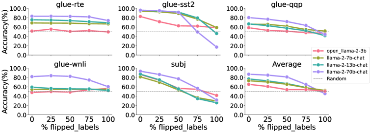
Figure 1: Larger models are easier to be affected by noise (flipped labels) and override pretrained biases than smaller models for different datasets and model families (chat/with instruct turning). Accuracy is calculated over 1000 evaluation prompts per dataset and over 5 runs with different random seeds for each evaluation, using $M=16$ in-context exemplars.

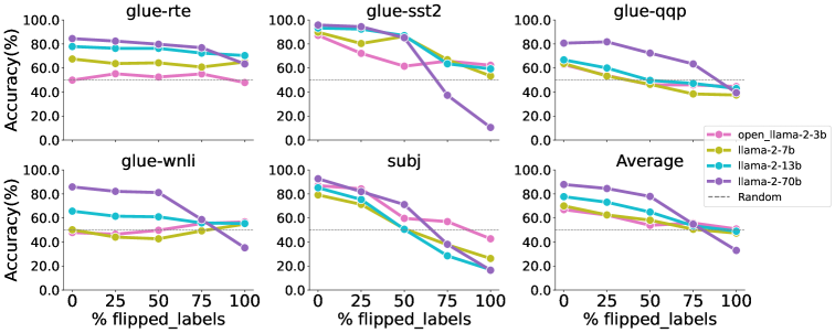
Figure 2: Larger models are easier to be affected by noise (flipped labels) and override pretrained biases than smaller models for different datasets and model families (original/without instruct turning). Accuracy is calculated over 1000 evaluation prompts per dataset and over 5 runs with different random seeds for each evaluation, using $M=16$ in-context exemplars.

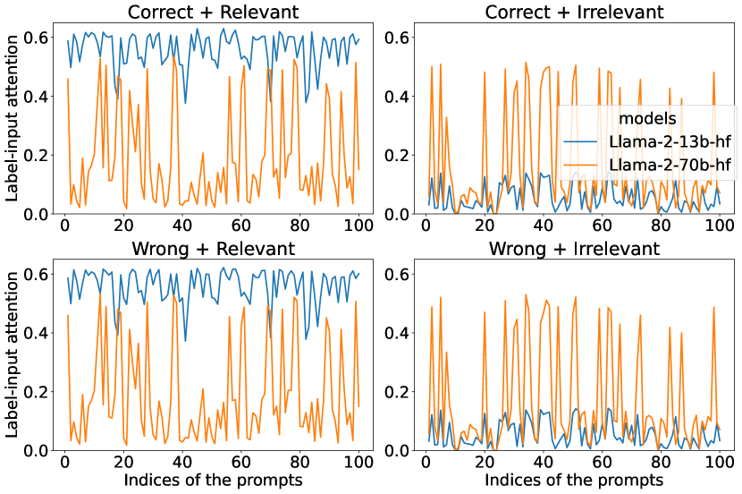
Figure 3: The magnitude of attention between the labels and input sentences in Llama 2-13b and 70b on 100 evaluation prompts; see the main text for the details. $x$-axis: indices of the prompts. $y$-axis: the norm of the last row of attention maps in the final layer. Correct: original label; wrong: flipped label; relevant: original input sentence; irrelevant: irrelevant sentence from other datasets. The results show that larger models focus on both sentences, while smaller models only focus on relevant sentences.

5.2 Behavior Difference

Similar to 4.3, to illustrate our insights, we will consider a setting where the smaller model learns useful features for the evaluation task while the larger model covers extra features. That is, for evaluation, we uniformly draw a task $\mathbf{t}_{\tau}=(i_{\tau},j_{\tau})$ from $S_{1}$, and then draw $M$ samples to form the evaluation prompt in the same way as during pretraining. To present our theorem (proved in Section C.2 using 5.1), we introduce some notations. Let

$$\mathbf{D}_{1}=\big{[}\operatorname*{diag}(\mathbf{V}^{*,(1)}),\dots,\operatorname*{diag}(\mathbf{V}^{*,(\nu_{1})}),\operatorname*{diag}(\mathbf{V}^{*,(\nu_{2}+1)}),$$

$$\dots,\operatorname*{diag}(\mathbf{V}^{*,(\nu_{2}+\nu_{1}+1)}),\operatorname*{diag}(\mathbf{V}^{*,(2\nu_{2}+2)})\big{]}\in\mathbb{R}^{d\times 2(\nu_{1}+1)}$$

$$\mathbf{D}_{2}=\left[\operatorname*{diag}(\mathbf{V}^{*,(1)}),\dots,\operatorname*{diag}(\mathbf{V}^{*,(2\nu_{2}+2)})\right]\in\mathbb{R}^{d\times 2(\nu_{2}+1)},$$

where for any $i\in[2(\nu_{2}+1)]$, $\mathbf{V}^{*,(i)}$ is defined in 5.1. Let $\hat{\phi}_{\tau,q}\in\mathbb{R}^{d}$ satisfy $\hat{\phi}_{\tau,q,i_{\tau}}={\phi}_{\tau,q,i_{\tau}},\hat{\phi}_{\tau,q,j_{\tau}}={\phi}_{\tau,q,j_{\tau}}$ and all other entries being zero. For a matrix $\mathbf{Z}$ and a vector $\mathbf{v}$, let $P_{\mathbf{Z}}$ denote the projection of $\mathbf{v}$ to the space of $\mathbf{Z}$, i.e., $P_{\mathbf{Z}}(\mathbf{v})=\mathbf{Z}(\mathbf{Z}^{\top}\mathbf{Z})^{-1}\mathbf{Z}^{\top}\mathbf{v}$.

Implications. 5.2 shows that during evaluation, we can decompose the input into two parts: signal and noise. Both the larger model and smaller model can capture the signal part well. However, the smaller model has a much smaller influence from noise than the larger model, i.e., the ratio is ${\nu_{1}+1\over\nu_{2}+1}$. The reason is that smaller models emphasize important hidden features while larger ones cover more hidden features, and thus, smaller models are more robust to noise while larger ones are easily distracted, leading to different ICL behaviors. This again sheds light on where transformers pay attention to and how that affects ICL.

Remark 5.1.

Here, we provide a detailed intuition about 5.2. $\Xi$ is the input noise. When we only care about the noise part, we can rewrite the smaller model as $g_{1}=h(\theta_{1},P_{D_{1}}(\Xi))$, and the larger model as $g_{2}=h(\theta_{2},P_{D_{2}}(\Xi))$, where they share the same $h$ function. Our conclusion says that $E[\|P_{D_{1}}(\Xi)\|_{2}^{2}]/E[\|P_{D_{2}}(\Xi)\|_{2}^{2}]=(\nu_{1}+1)/(\nu_{2}+1)$, which means the smaller model’s “effect” input noise is smaller than the larger model’s “effect” input noise. Although their original input noise is the same, as the smaller model only focuses on limited features, the smaller model will ignore part of the noise, and the “effect” input noise is small. However, the larger model is the opposite.

6 Experiments

Brilliant recent work (Wei et al., 2023b) runs intensive and thorough experiments to show that larger language models do in-context learning differently. Following their idea, we conduct similar experiments on binary classification datasets, which is consistent with our problem setting in the parity case, to support our theory statements.

Experimental setup. Following the experimental protocols in Wei et al. (2023b); Min et al. (2022), we conduct experiments on five prevalent NLP tasks, leveraging datasets from GLUE (Wang et al., 2018) tasks and Subj (Conneau & Kiela, 2018). Our experiments utilize various sizes of the Llama model families (Touvron et al., 2023a, b): 3B, 7B, 13B, 70B. We follow the prior work on in-context learning (Wei et al., 2023b) and use $M=16$ in-context exemplars. We aim to assess the models’ ability to use inherent semantic biases from pretraining when facing in-context examples. As part of this experiment, we introduce noise by inverting an escalating percentage of in-context example labels. To illustrate, a 100% label inversion for the SST-2 dataset implies that every “positive” exemplar is now labeled “negative”. Note that while we manipulate the in-context example labels, the evaluation sample labels remain consistent. We use the same templates as (Min et al., 2021), a sample evaluation for SST-2 when $M=2$:

sentence: show us a good time
The answer is positive.

sentence: as dumb and cheesy
The answer is negative.

sentence: it ’s a charming and often
affecting journey
The answer is

6.1 Behavior Difference

Figure 1 shows the result of model performance (chat/with instruct turning) across all datasets with respect to the proportion of labels that are flipped. When 0% label flips, we observe that larger language models have better in-context abilities. On the other hand, the performance decrease facing noise is more significant for larger models. As the percentage of label alterations increases, which can be viewed as increasing label noise $\sigma^{2}$, the performance of small models remains flat and seldom is worse than random guessing while large models are easily affected by the noise, as predicted by our analysis. These results indicate that large models can override their pretraining biases in-context input-label correlations, while small models may not and are more robust to noise. This observation aligns with the findings in Wei et al. (2023b) and our analysis.

We can see a similar or even stronger phenomenon in Figure 2: larger models are more easily affected by noise (flipped labels) and override pretrained biases than smaller models for the original/without instruct turning version (see the “Average” sub-figure). On the one hand, we conclude that both large base models and large chat models suffer from ICL robustness issues. On the other hand, this is also consistent with recent work suggesting that instruction tuning will impair LLM’s in-context learning capability.

6.2 Ablation Study

To further verify our analysis, we provide an ablation study. We concatenate an irrelevant sentence from GSM-IC (Shi et al., 2023a) to an input-label pair sentence from SST-2 in GLUE dataset. We use “correct” to denote the original label and “wrong” to denote the flipped label. Then, we measure the magnitude of correlation between label-input, by computing the norm of the last row of attention maps across all heads in the final layer. We do this between “correct”/“wrong” labels and the original/irrelevant inserted sentences. Figure 3 shows the results on 100 evaluation prompts; for example, the subfigure Correct+Relevant shows the correlation magnitude between the “correct” label and the original input sentence in each prompt. The results show that the small model Llama 2-13b mainly focuses on the relevant part (original input) and may ignore the irrelevant sentence, while the large model Llama 2-70b focuses on both sentences. This well aligns with our analysis.

7 More Discussions about Noise

There are three kinds of noise covered in our analysis:

Pretraining noise. We can see it as toxic or harmful pretraining data on the website (noisy training data). The model will learn these features and patterns. It is covered by $\xi$ in the linear regression case and $S_{2}$ in the parity case.

Input noise during inference. We can see it as natural noise as the user’s wrong spelling or biased sampling. It is a finite sampling error as $x$ drawn from the Gaussian distribution for the linear regression case and a finite sampling error as $x$ drawn from a uniform distribution for the parity case.

Label noise during inference. We can see it as adversarial examples, or misleading instructions, e.g., deliberately letting a model generate a wrong fact conclusion or harmful solution, e.g., poison making. It is $\sigma$ in the linear regression case and $S_{2}$ in the parity case.

For pretraining noise, it will induce the model to learn noisy or harmful features. During inference, for input noise and label noise, the larger model will pay additional attention to these noisy or harmful features in the input and label pair, i.e., $y\cdot x$, so that the input and label noise may cause a large perturbation in the final results. If there is no pretraining noise, then the larger model will have as good robustness as the smaller model. Also, if there is no input and label noise, the larger model will have as good robustness as the smaller model. The robustness gap only happens when both pretraining noise and inference noise exist simultaneously.

8 Conclusion

In this work, we answered our research question: why do larger language models do in-context learning differently? Our theoretical study showed that smaller models emphasize important hidden features while larger ones cover more hidden features, and thus the former are more robust to noise while the latter are more easily distracted, leading to different behaviors during in-context learning. Our empirical results provided positive support for the theoretical analysis. Our findings can help improve understanding of LLMs and ICL, and better training and application of these models.

Impact Statement

Our work aims to improve the understanding of the in-context learning mechanism and to inspire efficient and safe use of ICL. Our paper is purely theoretical and empirical in nature and thus we foresee no immediate negative ethical impact. We hope our work will inspire effective algorithm design and promote a better understanding of large language model learning mechanisms.

Appendix

Appendix A Limitations

We study and understand an interesting phenomenon of in-context learning: smaller models are more robust to noise, while larger ones are more easily distracted, leading to different ICL behaviors. Although we study two stylized settings and give the closed-form solution, our analysis cannot extend to real Transformers easily due to the high non-convex function and complicated design of multiple-layer Transformers. Also, our work does not study optimization trajectory, which we leave as future work. On the other hand, we use simple binary classification real-world datasets to verify our analysis, which still has a gap for the practical user using the LLM scenario.

Appendix B Deferred Proof for Linear Regression

B.1 Proof of 4.1

Here, we provide the proof of 4.1.

See 4.1

Proof of 4.1.

Note that,

$$\operatorname*{argmin}_{\mathbf{U}\in\mathbb{R}^{d\times d},\operatorname*{rank}(\mathbf{U})\leq r,u\in\mathbb{R}}\tilde{\ell}(\mathbf{U},u)= \operatorname*{argmin}_{\mathbf{U}\in\mathbb{R}^{d\times d},\operatorname*{rank}(\mathbf{U})\leq r,u\in\mathbb{R}}\tilde{\ell}(\mathbf{U},u)-\min_{\mathbf{U}\in\mathbb{R}^{d\times d},u\in\mathbb{R}}\tilde{\ell}(\mathbf{U},u)$$

$$= \operatorname*{argmin}_{\mathbf{U}\in\mathbb{R}^{d\times d},\operatorname*{rank}(\mathbf{U})\leq r,u\in\mathbb{R}}\left(\tilde{\ell}(\mathbf{U},u)-\min_{\mathbf{U}\in\mathbb{R}^{d\times d},u\in\mathbb{R}}\tilde{\ell}(\mathbf{U},u)\right).$$

Thus, we may consider Equation 7 in Lemma B.1 only. On the other hand, we have

$$\Gamma= \left(1+{1\over N}\right)\Lambda+{1\over N}\operatorname*{tr}(\Lambda)I_{d\times d}$$

$$= \left(1+{1\over N}\right)\mathbf{Q}\mathbf{D}\mathbf{Q}^{\top}+{1\over N}\operatorname*{tr}(\mathbf{D})\mathbf{Q}I_{d\times d}\mathbf{Q}^{\top}$$

$$= \mathbf{Q}\left(\left(1+{1\over N}\right)\mathbf{D}+{1\over N}\operatorname*{tr}(\mathbf{D})I_{d\times d}\right)\mathbf{Q}^{\top}.$$

We denote $\mathbf{D}^{\prime}=\left(1+{1\over N}\right)\mathbf{D}+{1\over N}\operatorname*{tr}(\mathbf{D})I_{d\times d}$. We can see $\Lambda^{1\over 2}=\mathbf{Q}{\mathbf{D}}^{1\over 2}\mathbf{Q}^{\top}$, $\Gamma^{1\over 2}=\mathbf{Q}{\mathbf{D}^{\prime}}^{1\over 2}\mathbf{Q}^{\top}$, and $\Gamma^{-1}=\mathbf{Q}{\mathbf{D}^{\prime}}^{-1}\mathbf{Q}^{\top}$. We denote $\mathbf{V}=u\mathbf{Q}^{\top}\mathbf{U}\mathbf{Q}$. Since $\Gamma$ and $\Lambda$ are commutable and the Frobenius norm ($F$-norm) of a matrix does not change after multiplying it by an orthonormal matrix, we have Equation 7 as

$$\tilde{\ell}(\mathbf{U},u)-\min_{\mathbf{U}\in\mathbb{R}^{d\times d},u\in\mathbb{R}}\tilde{\ell}(\mathbf{U},u)= {1\over 2}\left\|\Gamma^{1\over 2}\left(u\Lambda^{1\over 2}\mathbf{U}\Lambda^{1\over 2}-\Lambda\Gamma^{-1}\right)\right\|_{F}^{2}$$

$$= {1\over 2}\left\|\Gamma^{1\over 2}\Lambda^{1\over 2}\left(u\mathbf{U}-\Gamma^{-1}\right)\Lambda^{1\over 2}\right\|_{F}^{2}$$

$$= {1\over 2}\left\|{\mathbf{D}^{\prime}}^{1\over 2}{\mathbf{D}}^{1\over 2}\left({\mathbf{V}}-{\mathbf{D}^{\prime}}^{-1}\right){\mathbf{D}}^{1\over 2}\right\|_{F}^{2}.$$

As $\mathbf{W}^{KQ}$ is a matrix whose rank is at most $r$, we have $\mathbf{V}$ is also at most rank $r$. Then, we denote $\mathbf{V}^{*}=\operatorname*{argmin}_{\mathbf{V}\in\mathbb{R}^{d\times d},\operatorname*{rank}(\mathbf{V})\leq r}\left\|{\mathbf{D}^{\prime}}^{1\over 2}{\mathbf{D}}^{1\over 2}\left({\mathbf{V}}-{\mathbf{D}^{\prime}}^{-1}\right){\mathbf{D}}^{1\over 2}\right\|_{F}^{2}$. We can see that $\mathbf{V}^{*}$ is a diagonal matrix. Denote $\mathbf{D}^{\prime}=\operatorname*{diag}([\lambda_{1}^{\prime},\dots,\lambda_{d}^{\prime}])$ and $\mathbf{V}^{*}=\operatorname*{diag}([v^{*}_{1},\dots,v^{*}_{d}])$. Then, we have

$$\left\|{\mathbf{D}^{\prime}}^{1\over 2}{\mathbf{D}}^{1\over 2}\left({\mathbf{V}}-{\mathbf{D}^{\prime}}^{-1}\right){\mathbf{D}}^{1\over 2}\right\|_{F}^{2}$$ (4)

$$= \sum_{i=1}^{d}\left({\lambda_{i}^{\prime}}^{1\over 2}\lambda_{i}\left(v^{*}_{i}-{1\over{\lambda_{i}^{\prime}}}\right)\right)^{2}$$ (5)

$$= \sum_{i=1}^{d}\left(\left(1+{1\over N}\right)\lambda_{i}+{\operatorname*{tr}(\mathbf{D})\over N}\right)\lambda_{i}^{2}\left(v^{*}_{i}-{1\over{\left(1+{1\over N}\right)\lambda_{i}+{\operatorname*{tr}(\mathbf{D})\over N}}}\right)^{2}.$$ (6)

As $\mathbf{V}^{*}$ is the minimum rank $r$ solution, we have that $v^{*}_{i}\geq 0$ for any $i\in[d]$ and if $v^{*}_{i}>0$, we have $v^{*}_{i}={1\over{\left(1+{1\over N}\right)\lambda_{i}+{\operatorname*{tr}(\mathbf{D})\over N}}}$. Denote $g(x)=\left(\left(1+{1\over N}\right)x+{\operatorname*{tr}(\mathbf{D})\over N}\right)x^{2}\left({1\over{\left(1+{1\over N}\right)x+{\operatorname*{tr}(\mathbf{D})\over N}}}\right)^{2}=x^{2}\left({1\over{\left(1+{1\over N}\right)x+{\operatorname*{tr}(\mathbf{D})\over N}}}\right)$. It is easy to see that $g(x)$ is an increasing function on $[0,\infty)$. Now, we use contradiction to show that $\mathbf{V}^{*}$ only has non-zero entries in the first $r$ diagonal entries. Suppose $i>r$, such that $v^{*}_{i}>0$, then we must have $j\leq r$ such that $v^{*}_{j}=0$ as $\mathbf{V}^{*}$ is a rank $r$ solution. We find that if we set $v^{*}_{i}=0,v^{*}_{j}={1\over{\left(1+{1\over N}\right)\lambda_{j}+{\operatorname*{tr}(\mathbf{D})\over N}}}$ and all other values remain the same, Equation 6 will strictly decrease as $g(x)$ is an increasing function on $[0,\infty)$. Thus, here is a contradiction. We finish the proof by $\mathbf{V}^{*}=u\mathbf{Q}^{\top}\mathbf{U}^{*}\mathbf{Q}$. ∎

B.2 Behavior Difference

See 4.2

Proof of 4.2.

By 4.1, w.l.o.g, letting $c=1$, the optimal rank-$r$ solution $f_{\textup{LSA},\theta}$ satisfies $\theta=(\mathbf{W}^{PV},\mathbf{W}^{KQ})$, and

$$\mathbf{W}^{*PV}=\begin{pmatrix}0_{d\times d}&0_{d}\\ 0_{d}^{\top}&1\end{pmatrix},\mathbf{W}^{*KQ}=\begin{pmatrix}\mathbf{U}^{*}&0_{d}\\ 0_{d}^{\top}&0\end{pmatrix},$$

where $\mathbf{U}^{*}=\mathbf{Q}\mathbf{V}^{*}\mathbf{Q}^{\top}$.

We can see that $\mathbf{U}^{*}$ and $\Lambda$ commute. Denote $\widehat{\Lambda}:={1\over M}\sum_{i=1}^{M}\mathbf{x}_{i}\mathbf{x}_{i}^{\top}$. Note that we have

$$\widehat{y}_{q}= f_{\textup{LSA},\theta}(\widehat{\mathbf{E}})$$

$$= \begin{pmatrix}0_{d\times d}&0_{d}\\ 0_{d}^{\top}&1\end{pmatrix}\left({\widehat{\mathbf{E}}\widehat{\mathbf{E}}^{\top}\over M}\right)\begin{pmatrix}\mathbf{U}^{*}&0_{d}\\ 0_{d}^{\top}&0\end{pmatrix}\mathbf{x}_{q}$$

$$= \begin{pmatrix}0_{d\times d}&0_{d}\\ 0_{d}^{\top}&1\end{pmatrix}\begin{pmatrix}{1\over M}\left(\mathbf{x}_{q}\mathbf{x}_{q}^{\top}+\sum_{i=1}^{M}\mathbf{x}_{i}\mathbf{x}_{i}^{\top}\right)&{1\over M}\left(\sum_{i=1}^{M}\mathbf{x}_{i}\mathbf{x}_{i}^{\top}\mathbf{w}+\sum_{i=1}^{M}\epsilon_{i}\mathbf{x}_{i}\right)\\ {1\over M}\left(\sum_{i=1}^{M}\mathbf{w}^{\top}\mathbf{x}_{i}\mathbf{x}_{i}^{\top}+\sum_{i=1}^{M}\epsilon_{i}\mathbf{x}_{i}^{\top}\right)&{1\over M}\sum_{i=1}^{M}(\mathbf{w}^{\top}\mathbf{x}_{i}+\epsilon_{i})^{2}\end{pmatrix}$$

$$\cdot\begin{pmatrix}\mathbf{U}^{*}&0_{d}\\ 0_{d}^{\top}&0\end{pmatrix}\mathbf{x}_{q}$$

$$= \left(\mathbf{w}^{\top}\widehat{\Lambda}+{1\over M}\sum_{i=1}^{M}\epsilon_{i}\mathbf{x}_{i}^{\top}\right)\mathbf{U}^{*}\mathbf{x}_{q}.$$

Then, we have

$$\mathbb{E}_{\mathbf{x}_{1},\epsilon_{1},\dots,\mathbf{x}_{M},\epsilon_{M},\mathbf{x}_{q}}\left(\widehat{y}_{q}-\left\langle\mathbf{w},\mathbf{x}_{q}\right\rangle\right)^{2}$$

$$= \mathbb{E}_{\mathbf{x}_{1},\epsilon_{1},\dots,\mathbf{x}_{M},\epsilon_{M},\mathbf{x}_{q}}\left(\mathbf{w}^{\top}\widehat{\Lambda}\mathbf{U}^{*}\mathbf{x}_{q}+{1\over M}\sum_{i=1}^{M}\epsilon_{i}\mathbf{x}_{i}^{\top}\mathbf{U}^{*}\mathbf{x}_{q}-{\mathbf{w}^{\top}\mathbf{x}_{q}}\right)^{2}$$

$$= \underbrace{\mathbb{E}\left[\left(\mathbf{w}^{\top}\widehat{\Lambda}\mathbf{U}^{*}\mathbf{x}_{q}-{\mathbf{w}^{\top}\mathbf{x}_{q}}\right)^{2}\right]}_{\text{(I)}}+\underbrace{\mathbb{E}\left[\left({1\over M}\sum_{i=1}^{M}\epsilon_{i}\mathbf{x}_{i}^{\top}\mathbf{U}^{*}\mathbf{x}_{q}\right)^{2}\right]}_{\text{(II)}},$$

where the last equality is due to i.i.d. of $\epsilon_{i}$. We see that the label noise can only have an effect in the second term. For the term (I) we have,

$$\text{(I)}= \mathbb{E}\left[\left(\mathbf{w}^{\top}\widehat{\Lambda}\mathbf{U}^{*}\mathbf{x}_{q}-\mathbf{w}^{\top}\Lambda\mathbf{U}^{*}\mathbf{x}_{q}+\mathbf{w}^{\top}\Lambda\mathbf{U}^{*}\mathbf{x}_{q}-{\mathbf{w}^{\top}\mathbf{x}_{q}}\right)^{2}\right]$$

$$= \underbrace{\mathbb{E}\left[\left(\mathbf{w}^{\top}\widehat{\Lambda}\mathbf{U}^{*}\mathbf{x}_{q}-\mathbf{w}^{\top}\Lambda\mathbf{U}^{*}\mathbf{x}_{q}\right)^{2}\right]}_{\text{(III)}}+\underbrace{\mathbb{E}\left[\left(\mathbf{w}^{\top}\Lambda\mathbf{U}^{*}\mathbf{x}_{q}-{\mathbf{w}^{\top}\mathbf{x}_{q}}\right)^{2}\right]}_{\text{(IV)}},$$

where the last equality is due to $\mathbb{E}[\widehat{\Lambda}]=\Lambda$ and $\widehat{\Lambda}$ is independent with $\mathbf{x}_{q}$. Note the fact that $\mathbf{U}^{*}$ and $\Lambda$ commute. For the (III) term, we have

$$\text{(III)}= \mathbb{E}\left[\mathbb{E}\left[\left(\mathbf{w}^{\top}\widehat{\Lambda}\mathbf{U}^{*}\mathbf{x}_{q}\right)^{2}+\left(\mathbf{w}^{\top}\Lambda\mathbf{U}^{*}\mathbf{x}_{q}\right)^{2}-2\left(\mathbf{w}^{\top}\widehat{\Lambda}\mathbf{U}^{*}\mathbf{x}_{q}\right)\left(\mathbf{w}^{\top}\Lambda\mathbf{U}^{*}\mathbf{x}_{q}\right)\right]\middle|\mathbf{x}_{q}\right]$$

$$= \mathbb{E}\left[\left(\mathbf{w}^{\top}\widehat{\Lambda}\mathbf{U}^{*}\mathbf{x}_{q}\right)^{2}-\left(\mathbf{w}^{\top}\Lambda\mathbf{U}^{*}\mathbf{x}_{q}\right)^{2}\right].$$

By the property of trace, we have,

$$\text{(III)}= \mathbb{E}\left[\operatorname*{tr}\left(\widehat{\Lambda}\mathbf{w}\mathbf{w}^{\top}\widehat{\Lambda}(\mathbf{U}^{*})^{2}\Lambda\right)\right]-\|\mathbf{w}\|_{(\mathbf{U}^{*})^{2}\Lambda^{3}}^{2}$$

$$= \mathbb{E}\left[{1\over M^{2}}\operatorname*{tr}\left(\left(\sum_{i=1}^{M}\mathbf{x}_{i}\mathbf{x}_{i}^{\top}\right)\mathbf{w}\mathbf{w}^{\top}\left(\sum_{i=1}^{M}\mathbf{x}_{i}\mathbf{x}_{i}^{\top}\right)(\mathbf{U}^{*})^{2}\Lambda\right)\right]-\|\mathbf{w}\|_{(\mathbf{U}^{*})^{2}\Lambda^{3}}^{2}$$

$$= \mathbb{E}\left[{M-1\over M}\operatorname*{tr}\left(\Lambda\mathbf{w}\mathbf{w}^{\top}\Lambda(\mathbf{U}^{*})^{2}\Lambda\right)+{1\over M}\operatorname*{tr}\left(\mathbf{x}_{1}\mathbf{x}_{1}^{\top}\mathbf{w}\mathbf{w}^{\top}\mathbf{x}_{1}\mathbf{x}_{1}^{\top}(\mathbf{U}^{*})^{2}\Lambda\right)\right]-\|\mathbf{w}\|_{(\mathbf{U}^{*})^{2}\Lambda^{3}}^{2}$$

$$= -{1\over M}\|\mathbf{w}\|_{(\mathbf{U}^{*})^{2}\Lambda^{3}}^{2}+{1\over M}\mathbb{E}\left[\operatorname*{tr}\left(\mathbf{x}_{1}\mathbf{x}_{1}^{\top}\mathbf{w}\mathbf{w}^{\top}\mathbf{x}_{1}\mathbf{x}_{1}^{\top}(\mathbf{U}^{*})^{2}\Lambda\right)\right]$$

$$= -{1\over M}\|\mathbf{w}\|_{(\mathbf{U}^{*})^{2}\Lambda^{3}}^{2}+{1\over M}\mathbb{E}\left[\operatorname*{tr}\left(\left(\|\mathbf{w}\|_{\Lambda}^{2}\Lambda+2\Lambda\mathbf{w}^{\top}\mathbf{w}\Lambda\right)(\mathbf{U}^{*})^{2}\Lambda\right)\right]$$

$$= {1\over M}\|\mathbf{w}\|_{(\mathbf{U}^{*})^{2}\Lambda^{3}}^{2}+{1\over M}\|\mathbf{w}\|_{\Lambda}^{2}\operatorname*{tr}\left((\mathbf{U}^{*})^{2}\Lambda^{2}\right),$$

where the third last equality is by Lemma B.2. Furthermore, injecting $\mathbf{w}=\mathbf{Q}(\mathbf{s}+\xi)$, as $\xi^{\top}\mathbf{V}^{*}$ is a zero vector, we have

(III) $$={1\over M}\|\mathbf{s}+\xi\|_{(\mathbf{V}^{*})^{2}\mathbf{D}^{3}}^{2}+{1\over M}\|\mathbf{s}+\xi\|_{\mathbf{D}}^{2}\operatorname*{tr}\left((\mathbf{V}^{*})^{2}\mathbf{D}^{2}\right)$$

$$={1\over M}\|\mathbf{s}\|_{(\mathbf{V}^{*})^{2}\mathbf{D}^{3}}^{2}+{1\over M}\|\mathbf{s}+\xi\|_{\mathbf{D}}^{2}\operatorname*{tr}\left((\mathbf{V}^{*})^{2}\mathbf{D}^{2}\right).$$

Similarly, for the term (IV), we have

$$\text{(IV)}= \mathbb{E}\left[\left((\mathbf{s}+\xi)^{\top}\mathbf{Q}^{\top}\Lambda\mathbf{U}^{*}\mathbf{x}_{q}-{(\mathbf{s}+\xi)^{\top}\mathbf{Q}^{\top}\mathbf{x}_{q}}\right)^{2}\right]$$

$$= \mathbb{E}\left[\left(\mathbf{s}^{\top}\mathbf{D}\mathbf{V}^{*}\mathbf{Q}^{\top}\mathbf{x}_{q}-{\mathbf{s}^{\top}\mathbf{Q}^{\top}\mathbf{x}_{q}}-{\xi^{\top}\mathbf{Q}^{\top}\mathbf{x}_{q}}\right)^{2}\right]$$

$$= \mathbf{s}^{\top}(\mathbf{V}^{*})^{2}\mathbf{D}^{3}\mathbf{s}+\mathbf{s}^{\top}\mathbf{D}\mathbf{s}+\xi^{\top}\mathbf{D}\xi-2\mathbf{s}^{\top}\mathbf{V}^{*}\mathbf{D}^{2}\mathbf{s}$$

$$= \xi^{\top}\mathbf{D}\xi+\sum_{i\in[r]}\mathbf{s}_{i}^{2}\lambda_{i}\left(\lambda_{i}^{2}(v^{*}_{i})^{2}-2\lambda_{i}v^{*}_{i}+1\right)$$

$$= \|\xi\|_{\mathbf{D}}^{2}+\sum_{i\in[r]}\mathbf{s}_{i}^{2}\lambda_{i}\left(\lambda_{i}v^{*}_{i}-1\right)^{2},$$

where the third equality is due to $\mathbf{s}^{\top}\mathbf{A}\xi=0$ for any diagonal matrix $\mathbf{A}\in\mathbb{R}^{d\times d}$.

Now, we analyze the label noise term. By $\mathbf{U}^{*}$ and $\Lambda$ being commutable, for the term (II), we have

$$\text{(II)}= {\sigma^{2}\over M^{2}}\mathbb{E}\left[\left(\sum_{i=1}^{M}\mathbf{x}_{i}^{\top}\mathbf{U}^{*}\mathbf{x}_{q}\right)^{2}\right]$$

$$= {\sigma^{2}\over M^{2}}\mathbb{E}\left[\operatorname*{tr}\left(\left(\sum_{i=1}^{M}\mathbf{x}_{i}\right)^{\top}\mathbf{U}^{*}\Lambda\mathbf{U}^{*}\left(\sum_{i=1}^{M}\mathbf{x}_{i}\right)\right)\right]$$

$$= {\sigma^{2}\over M}\mathbb{E}\left[\operatorname*{tr}\left(\mathbf{x}_{1}^{\top}\mathbf{U}^{*}\Lambda\mathbf{U}^{*}\mathbf{x}_{1}\right)\right]$$

$$= {\sigma^{2}\over M}\operatorname*{tr}\left((\mathbf{V}^{*})^{2}\mathbf{D}^{2}\right),$$

where all cross terms vanish in the second equality. We conclude by combining four terms. ∎

See 4.3

Proof of 4.3.

Let $\mathbf{V}^{*}=\operatorname*{diag}([v^{*}_{1},\dots,v^{*}_{d}])$ satisfying for any $i\leq{r},v^{*}_{i}={N\over{\left(N+1\right)\lambda_{i}+{\operatorname*{tr}(\mathbf{D})}}}$ and for any $i>{r},v^{*}_{i}=0$. Let ${\mathbf{V}^{\prime}}^{*}=\operatorname*{diag}([{v^{\prime}}^{*}_{1},\dots,{v^{\prime}}^{*}_{d}])$ be satisfied for any $i\leq{r^{\prime}},{v^{\prime}}^{*}_{i}={N\over{\left(N+1\right)\lambda_{i}+{\operatorname*{tr}(\mathbf{D})}}}$ and for any $i>{r^{\prime}},{v^{\prime}}^{*}_{i}=0$. Note that $\mathbf{V}^{*}$ is a truncated diagonal matrix of ${\mathbf{V}^{\prime}}^{*}$. By 4.1 and 4.2, we have

$$\mathcal{L}(f_{2};\widehat{\mathbf{E}})-\mathcal{L}(f_{1};\widehat{\mathbf{E}})= \left({1\over M}\|\mathbf{s}\|_{({\mathbf{V}^{\prime}}^{*})^{2}\mathbf{D}^{3}}^{2}+{1\over M}\left(\|\mathbf{s}\|_{\mathbf{D}}^{2}+\sigma^{2}\right)\operatorname*{tr}\left(({\mathbf{V}^{\prime}}^{*})^{2}\mathbf{D}^{2}\right)+\sum_{i\in[{r^{\prime}}]}\mathbf{s}_{i}^{2}\lambda_{i}\left(\lambda_{i}{v^{\prime}}^{*}_{i}-1\right)^{2}\right)$$

$$-\left({1\over M}\|\mathbf{s}\|_{(\mathbf{V}^{*})^{2}\mathbf{D}^{3}}^{2}+{1\over M}\left(\|\mathbf{s}\|_{\mathbf{D}}^{2}+\sigma^{2}\right)\operatorname*{tr}\left((\mathbf{V}^{*})^{2}\mathbf{D}^{2}\right)+\sum_{i\in[{r}]}\mathbf{s}_{i}^{2}\lambda_{i}\left(\lambda_{i}v^{*}_{i}-1\right)^{2}\right)$$

$$= {1\over M}\left(\|\mathbf{s}\|_{\mathbf{D}}^{2}+\sigma^{2}\right)\left(\operatorname*{tr}\left(({\mathbf{V}^{\prime}}^{*})^{2}\mathbf{D}^{2}\right)-\operatorname*{tr}\left((\mathbf{V}^{*})^{2}\mathbf{D}^{2}\right)\right)$$

$$= {1\over M}\left(\|\mathbf{s}\|_{\mathbf{D}}^{2}+\sigma^{2}\right)\left(\sum_{i={r}+1}^{{r^{\prime}}}\left({N\lambda_{i}\over{\left(N+1\right)\lambda_{i}+{\operatorname*{tr}(\mathbf{D})}}}\right)^{2}\right).$$

∎

B.3 Auxiliary Lemma

Lemma B.1 provides the structure of the quadratic form of our MSE loss.

Lemma B.1 (Corollary A.2 in Zhang et al. (2023b)).

The loss function $\tilde{\ell}$ in Lemma 4.1 satisfies

$$\min_{\mathbf{U}\in\mathbb{R}^{d\times d},u\in\mathbb{R}}\tilde{\ell}(\mathbf{U},u)=-{1\over 2}\operatorname*{tr}[\Lambda^{2}\Gamma^{-1}],$$

where $\mathbf{U}=c\Gamma^{-1},u={1\over c}$ for any non-zero constant $c$ are minimum solution. We also have

$$\tilde{\ell}(\mathbf{U},u)-\min_{\mathbf{U}\in\mathbb{R}^{d\times d},u\in\mathbb{R}}\tilde{\ell}(\mathbf{U},u)={1\over 2}\left\|\Gamma^{1\over 2}\left(u\Lambda^{1\over 2}\mathbf{U}\Lambda^{1\over 2}-\Lambda\Gamma^{-1}\right)\right\|_{F}^{2}.$$ (7)

Lemma B.2.

Let $\mathbf{x}\sim\mathcal{N}(0,\Lambda),\epsilon\sim\mathcal{N}(0,\sigma^{2})$ and $y=\left\langle\mathbf{w},\mathbf{x}\right\rangle+\epsilon$, where $\mathbf{w}\in\mathbb{R}^{d}$ is a fixed vector. Then we have

$$\mathbb{E}\left[y^{2}\mathbf{x}\mathbf{x}^{\top}\right]= \sigma^{2}\Lambda+\|\mathbf{w}\|_{\Lambda}^{2}\Lambda+2\Lambda\mathbf{w}^{\top}\mathbf{w}\Lambda,$$

$$\mathbb{E}(y\mathbf{x})\mathbb{E}(y\mathbf{x})^{\top}= \Lambda^{\top}\mathbf{w}\mathbf{w}^{\top}\Lambda,$$

$$\mathbb{E}\left[(y\mathbf{x}-\mathbb{E}(y\mathbf{x}))(y\mathbf{x}-\mathbb{E}(y\mathbf{x}))^{\top}\right]= \sigma^{2}\Lambda+\|\mathbf{w}\|_{\Lambda}^{2}\Lambda+\Lambda\mathbf{w}^{\top}\mathbf{w}\Lambda.$$

Proof of Lemma B.2.

As $y$ is a zero mean Gaussian, by Isserlis’ theorem (Wick, 1950; Michalowicz et al., 2009), for any $i,j\in[d]$ we have

$$\mathbb{E}[y^{2}\mathbf{x}_{i}\mathbf{x}_{j}]= \mathbb{E}[y^{2}]\mathbb{E}[\mathbf{x}_{i}\mathbf{x}_{j}]+2\mathbb{E}[y\mathbf{x}_{i}]\mathbb{E}[y\mathbf{x}_{j}]$$

$$= \left(\sigma^{2}+\mathbf{w}^{\top}\Lambda\mathbf{w}\right)\Lambda_{i,j}+2\Lambda_{i}^{\top}\mathbf{w}\mathbf{w}^{\top}\Lambda_{j}.$$

Thus, we have $\mathbb{E}\left[y^{2}\mathbf{x}\mathbf{x}^{\top}\right]=\left(\sigma^{2}+\mathbf{w}^{\top}\Lambda\mathbf{w}\right)\Lambda+2\Lambda\mathbf{w}^{\top}\mathbf{w}\Lambda$. Similarly, we also have $\mathbb{E}(y\mathbf{x})\mathbb{E}(y\mathbf{x})^{\top}=\Lambda^{\top}\mathbf{w}\mathbf{w}^{\top}\Lambda$. Thus, we have

$$\mathbb{E}\left[(y\mathbf{x}-\mathbb{E}(y\mathbf{x}))(y\mathbf{x}-\mathbb{E}(y\mathbf{x}))^{\top}\right]$$

$$= \mathbb{E}\left[y^{2}\mathbf{x}\mathbf{x}^{\top}-y\mathbf{x}\mathbb{E}(y\mathbf{x})^{\top}-\mathbb{E}(y\mathbf{x})y\mathbf{x}^{\top}+\mathbb{E}(y\mathbf{x})\mathbb{E}(y\mathbf{x})^{\top}\right]$$

$$= \mathbb{E}\left[y^{2}\mathbf{x}\mathbf{x}^{\top}\right]-\mathbb{E}(y\mathbf{x})\mathbb{E}(y\mathbf{x})^{\top}$$

$$= \left(\sigma^{2}+\mathbf{w}^{\top}\Lambda\mathbf{w}\right)\Lambda+\Lambda\mathbf{w}^{\top}\mathbf{w}\Lambda.$$

∎

Appendix C Deferred Proof for Parity Classification

C.1 Proof of 5.1

Here, we provide the proof of 5.1. See 5.1

Proof of 5.1.

Recall $\mathbf{t}_{\tau}=(i_{\tau},j_{\tau})$. Let $\mathbf{z}_{\tau}\in\mathbb{R}^{d}$ satisfy $\mathbf{z}_{\tau,i_{\tau}}=\mathbf{z}_{\tau,j_{\tau}}=2\gamma$ and all other entries are zero. Denote $\mathbf{V}^{(i)}=\mathbf{G}^{\top}\mathbf{W}^{(i)}\mathbf{G}$. Notice that $\|\mathbf{W}^{(i)}\|_{F}^{2}=\|\mathbf{V}^{(i)}\|_{F}^{2}$. Thus, we denote $\mathbf{V}^{*,(i)}=\mathbf{G}^{\top}\mathbf{W}^{*,(i)}\mathbf{G}$. Then, we have

$$\mathbb{E}_{\tau}\left[\ell\left(y_{\tau,q}\cdot g(\mathbf{X}_{\tau},\mathbf{y}_{\tau},\mathbf{x}_{\tau,q})\right)\right]$$

$$= \mathbb{E}_{\tau}\left[\ell\left(y_{\tau,q}\left(\sum_{i\in[m]}\mathbf{a}_{i}\sigma\left[{\mathbf{y}_{\tau}^{\top}\mathbf{X}_{\tau}\over N}\mathbf{W}^{(i)}\mathbf{x}_{\tau,q}\right]\right)\right)\right]$$

$$= \mathbb{E}_{\tau}\left[\ell\left(y_{\tau,q}\left(\sum_{i\in[m]}\mathbf{a}_{i}\sigma\left[\mathbf{z}_{\tau}^{\top}\mathbf{V}^{(i)}\phi_{\tau,q}\right]\right)\right)\right]$$

$$= \mathbb{E}_{\tau}\left[\ell\left(y_{\tau,q}\left(\sum_{i\in[m]}\mathbf{a}_{i}\sigma\left[2\gamma(\mathbf{V}_{i_{\tau},:}^{(i)}+\mathbf{V}_{j_{\tau},:}^{(i)})\phi_{\tau,q}\right]\right)\right)\right].$$

We can see that for any $i\in[m],$ $|\mathbf{a}^{*}_{i}|=1$ and $\mathbf{V}_{j,l}^{*,(i)}=0$ when $j\neq l$. As ReLU is a homogeneous function, we have

$$\mathbb{E}_{\tau}\left[\ell\left(y_{\tau,q}\cdot g^{*}(\mathbf{X}_{\tau},\mathbf{y}_{\tau},\mathbf{x}_{\tau,q})\right)\right]$$

$$= \underbrace{(1-p_{\mathcal{T}})\mathbb{E}\left[\ell\left(2\gamma\phi_{\tau,q,i_{\tau}}\phi_{\tau,q,j_{\tau}}\left(\sum_{i\in[m]}\mathbf{a}^{*}_{i}\sigma\left[\mathbf{V}_{i_{\tau},i_{\tau}}^{*,(i)}\phi_{\tau,q,i_{\tau}}+\mathbf{V}_{j_{\tau},j_{\tau}}^{*,(i)}\phi_{\tau,q,j_{\tau}}\right]\right)\right)\middle|\mathbf{t}_{\tau}\in S_{1}\right]}_{\text{(I)}}$$

$$\quad~{}~{}+\underbrace{p_{\mathcal{T}}\mathbb{E}\left[\ell\left(2\gamma\phi_{\tau,q,i_{\tau}}\phi_{\tau,q,j_{\tau}}\left(\sum_{i\in[m]}\mathbf{a}^{*}_{i}\sigma\left[\mathbf{V}_{i_{\tau},i_{\tau}}^{*,(i)}\phi_{\tau,q,i_{\tau}}+\mathbf{V}_{j_{\tau},j_{\tau}}^{*,(i)}\phi_{\tau,q,j_{\tau}}\right]\right)\right)\middle|\mathbf{t}_{\tau}\in S_{2}\right]}_{\text{(II)}}.$$

We have

$$\text{(I)}= (1-p_{\mathcal{T}})\cdot\Bigg{\{}({1\over 4}+\gamma)\mathbb{E}\left[\ell\left(2\gamma\left(\sum_{i\in[m]}\mathbf{a}^{*}_{i}\sigma\left[\mathbf{V}_{i_{\tau},i_{\tau}}^{*,(i)}+\mathbf{V}_{j_{\tau},j_{\tau}}^{*,(i)}\right]\right)\right)\middle|\mathbf{t}_{\tau}\in S_{1}\right]$$

$$\quad\quad\quad\quad\quad+{1\over 4}\mathbb{E}\left[\ell\left(-2\gamma\left(\sum_{i\in[m]}\mathbf{a}^{*}_{i}\sigma\left[\mathbf{V}_{i_{\tau},i_{\tau}}^{*,(i)}-\mathbf{V}_{j_{\tau},j_{\tau}}^{*,(i)}\right]\right)\right)\middle|\mathbf{t}_{\tau}\in S_{1}\right]$$

$$\quad\quad\quad\quad\quad+({1\over 4}-\gamma)\mathbb{E}\left[\ell\left(2\gamma\left(\sum_{i\in[m]}\mathbf{a}^{*}_{i}\sigma\left[-\mathbf{V}_{i_{\tau},i_{\tau}}^{*,(i)}-\mathbf{V}_{j_{\tau},j_{\tau}}^{*,(i)}\right]\right)\right)\middle|\mathbf{t}_{\tau}\in S_{1}\right]$$

$$\quad\quad\quad\quad\quad+{1\over 4}\mathbb{E}\left[\ell\left(-2\gamma\left(\sum_{i\in[m]}\mathbf{a}^{*}_{i}\sigma\left[-\mathbf{V}_{i_{\tau},i_{\tau}}^{*,(i)}+\mathbf{V}_{j_{\tau},j_{\tau}}^{*,(i)}\right]\right)\right)\middle|\mathbf{t}_{\tau}\in S_{1}\right]\Bigg{\}}.$$

We can get a similar equation for (II).

We make some definitions to be used.

We define a pattern as $(z_{1},\{(i_{\tau},z_{2}),(j_{\tau},z_{3})\})$, where $z_{1},z_{2},z_{3}\in\{\pm 1\}$. We define a pattern is covered by a neuron means there exists $i\in[m]$, such that $\mathbf{a}^{*}_{i}=z_{1}$ and $\operatorname*{sign}(\mathbf{V}_{i_{\tau},i_{\tau}}^{*,(i)})=z_{2}$ and $\operatorname*{sign}(\mathbf{V}_{j_{\tau},j_{\tau}}^{*,(i)})=z_{3}$. We define a neuron as being positive when its $\mathbf{a}^{*}_{i}=+1$ and being negative when its $\mathbf{a}^{*}_{i}=-1$. We define a pattern as being positive if $z_{1}=+1$ and being negative if $z_{1}=-1$.

Then all terms in (I) and (II) can be written as:

$$\alpha\mathbb{E}\left[\ell\left(2\gamma z_{1}\left(\sum_{i\in[m]}\mathbf{a}^{*}_{i}\sigma\left[z_{2}\mathbf{V}_{i_{\tau},i_{\tau}}^{*,(i)}+z_{3}\mathbf{V}_{j_{\tau},j_{\tau}}^{*,(i)}\right]\right)\right)\right],$$

where $\alpha$ is the scalar term. Note that there are total ${k(k-1)\over 2}\times 4$ patterns in (I) and $\left({d(d-1)\over 2}-{k(k-1)\over 2}\right)\times 4$ patterns in (II). The loss depends on the weighted sum of non-covered patterns. To have zero loss, we need all patterns to be covered by $m$ neurons, i.e., $(\mathbf{a}^{*},\mathbf{V}^{*,(1)},\dots,\mathbf{V}^{*,(m)})$.

Note that one neuron at most cover ${d(d-1)\over 2}$ patterns. Also, by $0<p_{\mathcal{T}}<{{1\over 4}-\gamma\over{d(d-1)\over 2}({1\over 4}+\gamma)+{1\over 4}-\gamma}$, we have

$${d(d-1)\over 2}p_{\mathcal{T}}({1\over 4}+\gamma)<(1-p_{\mathcal{T}})({1\over 4}-\gamma),$$

which means the model will only cover all patterns in (I) before covering a pattern in (II) in purpose.

Now, we show that the minimum number of neurons to cover all patterns in (I) and (II) is $2(\nu_{2}+1)$.

First, we show that $2(\nu_{2}+1)$ neurons are enough to cover all patterns in (I) and (II).

For $i\in[\nu_{2}]$ and $i_{\tau}\in[d]$, $\mathbf{V}_{i_{\tau},i_{\tau}}^{(i)}=(2\operatorname*{digit}(\operatorname*{bin}(i_{\tau}-1),i)-1)/(4\gamma)$ and all non-diagonal entries in $\mathbf{V}^{(i)}$ being zero and $\mathbf{a}_{i}=-1$. For $i=\nu_{2}+1$ and $i_{\tau}\in[d]$, $\mathbf{V}_{i_{\tau},i_{\tau}}^{(i)}=-\nu_{2}/(4\gamma)$ and all non-diagonal entries in $\mathbf{V}^{(i)}$ being zero and $\mathbf{a}_{i}=+1$. For $i\in[2(\nu_{2}+1)]\setminus[\nu_{2}+1]$, let $\mathbf{V}^{(i)}=-\mathbf{V}^{(i-\nu_{2}-1)}$ and $\mathbf{a}_{i}=\mathbf{a}_{i-\nu_{2}-1}$.

We can check that this construction can cover all patterns in (I) and (II) and only needs $2(\nu_{2}+1)$ neurons. $\mathbf{V}^{(\nu_{2}+1)}$ and $\mathbf{V}^{(2(\nu_{2}+1))}$ cover all positive patterns. All other neurons cover all negative patterns. This is because $\operatorname*{bin}(i_{\tau})$ and $\operatorname*{bin}(j_{\tau})$ have at least one digit difference. If $\operatorname*{bin}(i_{\tau})$ and $\operatorname*{bin}(j_{\tau})$ are different in the $i$-th digit, then $(-1,\{(i_{\tau},-1),(j_{\tau},+1)\})$ and $(-1,\{(i_{\tau},+1),(j_{\tau},-1)\})$ are covered by the $i$-th and $i+\nu_{2}+1$-th neuron.

We can also check that the scalar ${1\over 4\gamma}$ and ${\nu_{2}\over 4\gamma}$ is the optimal value. Note that

1. For any negative patterns, the positive neurons will not have a cancellation effect on the negative neurons, i.e., when $y_{q}=-1$, the positive neurons will never activate.

2. For each negative neuron, there exist some patterns that are uniquely covered by it.

3. For any positive patterns, there are at most $\nu_{2}-1$ negative neurons that will have a cancellation effect on the positive neurons, i.e., when $y_{q}=+1$, these negative neurons will activate simultaneously. Also, we can check that there is a positive pattern such that there are $\nu_{2}-1$ negative neurons that will have a cancellation effect.

4. For two positive neurons, there exist some patterns that are uniquely covered by one of them.

Due to hinge loss, we can see that ${1\over 4\gamma}$ is tight for negative neurons as (1) and (2). Similarly, we can also see that ${\nu_{2}\over 4\gamma}$ is tight for positive neurons as (3) and (4).

Second, we prove that we need at least $2(\nu_{2}+1)$ neurons to cover all patterns in (I) and (II).

We can see that we need at least 2 positive neurons to cover all positive patterns. Then, we only need to show that $2\nu_{2}-1$ neurons are not enough to cover all negative patterns. We can prove that all negative patterns are covered equivalent to all numbers from $\{0,1,\dots,2^{\nu_{2}}-1\}$ are encoded by $\left\{\left(\mathbf{V}_{i,i}^{(1)},\dots,\mathbf{V}_{i,i}^{(\nu_{2})}\right)~{}\middle|~{}i\in[k]\right\}$. Then $2\nu_{2}-1$ is not enough to do so.

Therefore, the minimum number of neurons to cover all patterns in (I) and (II) is $2(\nu_{2}+1)$.

Thus, when $m=2(\nu_{1}+1)$, the optimal solution will cover all patterns in (I) but not all in (II). When $m\geq 2(\nu_{2}+1)$, the optimal solution will cover all patterns in (I) and (II). We see that $g^{*}_{1}$ neurons as the subset of $g^{*}_{2}$ neurons, while the only difference is that the scalar of positive neurons is ${\nu_{1}\over 4\gamma}$ for $g^{*}_{1}$ and ${\nu_{2}\over 4\gamma}$ for $g^{*}_{2}$. Thus, we finished the proof. ∎

C.2 Proof of 5.2

Here, we provide the proof of 5.2. See 5.2

Proof of 5.2.

Let $\Phi^{\tau}=[\phi_{\tau,1},\dots,\phi_{\tau,M}]^{\top}\in\mathbb{R}^{M\times d}$. Recall $\mathbf{t}_{\tau}=(i_{\tau},j_{\tau})$. Let $\mathbf{z}_{\tau}\in\mathbb{R}^{d}$ satisfy $\mathbf{z}_{\tau,i_{\tau}}=\mathbf{z}_{\tau,j_{\tau}}=2\gamma$ and all other entries are zero. We see $\mathbf{t}_{\tau}$ as an index set and let $\mathbf{r}_{\tau}=[d]\setminus\mathbf{t}_{\tau}$. Then, we have

$$g^{*}_{2}(\mathbf{X}_{\tau},\mathbf{y}_{\tau},\mathbf{x}_{\tau,q})$$

$$= \sum_{i\in[m]}\mathbf{a}^{*}_{i}\sigma\left[{\mathbf{y}_{\tau}^{\top}\mathbf{X}_{\tau}\over M}\mathbf{W}^{*,(i)}\mathbf{x}_{\tau,q}\right]$$

$$= \sum_{i\in[m]}\mathbf{a}^{*}_{i}\sigma\left[{\mathbf{y}_{\tau}^{\top}\Phi^{\tau}\over M}\mathbf{V}^{*,(i)}\phi_{\tau,q}\right]$$

$$= \sum_{i\in[m]}\mathbf{a}^{*}_{i}\sigma\left[{\mathbf{y}_{\tau}^{\top}\Phi^{\tau}_{:,\mathbf{t}_{\tau}}\over M}\mathbf{V}^{*,(i)}_{\mathbf{t}_{\tau},:}\phi_{\tau,q,\mathbf{t}_{\tau}}+{\mathbf{y}_{\tau}^{\top}\Phi^{\tau}_{:,\mathbf{r}_{\tau}}\over M}\mathbf{V}^{*,(i)}_{\mathbf{r}_{\tau},:}\phi_{\tau,q,\mathbf{r}_{\tau}}\right].$$

Note that we can absorb the randomness of $\mathbf{y}_{\tau},\Phi^{\tau}_{:,\mathbf{r}_{\tau}},\phi_{\tau,q,\mathbf{r}_{\tau}}$ together.

Let $z_{i}$ for $i\in[n]$ uniformly draw from $\{-1,+1\}$. By Chernoff bound for binomial distribution (Lemma C.1), for any $0<\epsilon<1$, we have

$$\Pr\left(\left|{\sum_{i\in[n]}z_{i}\over n}\right|\geq\epsilon\right)\leq 2\exp\left(-{\epsilon^{2}n\over 6}\right).$$

Thus, for any $0<\delta<1$, with probability at least $1-\delta$ over the randomness of evaluation data, such that

$$\left|\Xi_{\mathbf{t}_{\tau}}^{\top}\operatorname*{diag}(\mathbf{V}^{*,(i)}_{\mathbf{t}_{\tau},\mathbf{t}_{\tau}})\right|\leq O\left(\sqrt{{1\over M}\log{1\over\delta}}\right).$$

Then, for any $0<\delta<1$, with probability at least $1-\delta$ over the randomness of evaluation data, we have

$$g^{*}_{2}(\mathbf{X}_{\tau},\mathbf{y}_{\tau},\mathbf{x}_{\tau,q})$$

$$= \sum_{i\in[m]}\mathbf{a}^{*}_{i}\sigma\left[{\mathbf{y}_{\tau}^{\top}\Phi^{\tau}_{:,\mathbf{t}_{\tau}}\over M}\mathbf{V}^{*,(i)}_{\mathbf{t}_{\tau},:}\phi_{\tau,q,\mathbf{t}_{\tau}}+\Xi^{\top}\operatorname*{diag}(\mathbf{V}^{*,(i)})-\Xi_{\mathbf{t}_{\tau}}^{\top}\operatorname*{diag}(\mathbf{V}^{*,(i)}_{\mathbf{t}_{\tau},\mathbf{t}_{\tau}})\right]$$

$$= \sum_{i\in[m]}\mathbf{a}^{*}_{i}\sigma\left[\mathbf{z}_{\tau}^{\top}\mathbf{V}^{*,(i)}_{\mathbf{t}_{\tau},:}\phi_{\tau,q,\mathbf{t}_{\tau}}+\Xi^{\top}\operatorname*{diag}(\mathbf{V}^{*,(i)})-\Xi_{\mathbf{t}_{\tau}}^{\top}\operatorname*{diag}(\mathbf{V}^{*,(i)}_{\mathbf{t}_{\tau},\mathbf{t}_{\tau}})\right]$$

$$= \sum_{i\in[m]}\mathbf{a}^{*}_{i}\sigma\left[2\gamma\operatorname*{diag}\left(\mathbf{V}^{*,(i)}_{\mathbf{t}_{\tau},\mathbf{t}_{\tau}}\right)^{\top}\phi_{\tau,q,\mathbf{t}_{\tau}}+\Xi^{\top}\operatorname*{diag}(\mathbf{V}^{*,(i)})-\Xi_{\mathbf{t}_{\tau}}^{\top}\operatorname*{diag}(\mathbf{V}^{*,(i)}_{\mathbf{t}_{\tau},\mathbf{t}_{\tau}})\right]$$

$$= \sum_{i\in[m]}\mathbf{a}^{*}_{i}\sigma\left[\operatorname*{diag}\left(\mathbf{V}^{*,(i)}\right)^{\top}\left(2\gamma\hat{\phi}_{\tau,q}+\Xi\right)-\Xi_{\mathbf{t}_{\tau}}^{\top}\operatorname*{diag}(\mathbf{V}^{*,(i)}_{\mathbf{t}_{\tau},\mathbf{t}_{\tau}})\right]$$

$$= \sum_{i\in[m]}\mathbf{a}^{*}_{i}\sigma\left[\operatorname*{diag}\left(\mathbf{V}^{*,(i)}\right)^{\top}\left(2\gamma\hat{\phi}_{\tau,q}+\Xi\right)+O\left(\sqrt{{1\over M}\log{1\over\delta}}\right)\right]$$

$$= \sum_{i\in[m]}\mathbf{a}^{*}_{i}\sigma\left[\operatorname*{diag}\left(\mathbf{V}^{*,(i)}\right)^{\top}\left(2\gamma\hat{\phi}_{\tau,q}+P_{\mathbf{D}_{2}}(\Xi)\right)+O\left(\sqrt{{1\over M}\log{1\over\delta}}\right)\right]$$

$$= ~{}h(\theta_{2},2\gamma\hat{\phi}_{\tau,q}+P_{\mathbf{D}_{2}}(\Xi))+O\left(\sqrt{{\nu_{2}\over M}\log{1\over\delta}}\right).$$

Similarly, we have $g^{*}_{1}(\mathbf{X}_{\tau},\mathbf{y}_{\tau},\mathbf{x}_{\tau,q})=h(\theta_{1},2\gamma\hat{\phi}_{\tau,q}+P_{\mathbf{D}_{1}}(\Xi))+O\left(\sqrt{{\nu_{1}\over M}\log{1\over\delta}}\right)$.

As $\mathbf{t}_{\tau}\in S_{1}$ and the number of $(\phi_{i_{\tau}},\phi_{j_{\tau}})$ being balanced as training, by careful checking, we can see that $\ell(y_{q}\cdot h(\theta_{1},2\gamma\hat{\phi}_{\tau,q}))=\ell(y_{q}\cdot h(\theta_{2},2\gamma\hat{\phi}_{\tau,q}))=0$ and we have $2\gamma\hat{\phi}_{\tau,q}$ is the signal part.

On the other hand, we know that all the first half columns in $\mathbf{D}_{2}$ are orthogonal with each other, and the second half columns in $\mathbf{D}_{2}$ are opposite to the first half columns. We have the same fact to $\mathbf{D}_{1}$. As $\Xi$ is a symmetric noise distribution, we have ${\mathbb{E}[\|P_{\mathbf{D}_{1}}(\Xi))\|_{2}^{2}]\over\mathbb{E}[\|P_{\mathbf{D}_{2}}(\Xi))\|_{2}^{2}]}={\nu_{1}+1\over\nu_{2}+1}$ and we have $P_{\mathbf{D}_{1}}(\Xi))$ and $P_{\mathbf{D}_{2}}(\Xi))$ is the noise part. ∎

C.3 Auxiliary Lemma

Lemma C.1 (Chernoff bound for binomial distribution).

Let $Z\sim\operatorname*{Bin}(n,p)$ and let $\mu=\mathbb{E}[Z]$. For any $0<\epsilon<1$, we have

$$\Pr(|Z-\mu|\geq\epsilon\mu)\leq 2\exp\left(-{\epsilon^{2}\mu\over 3}\right).$$

References

• Agrawal et al. (2022) Agrawal, S., Zhou, C., Lewis, M., Zettlemoyer, L., and Ghazvininejad, M. In-context examples selection for machine translation. arXiv preprint arXiv:2212.02437, 2022.
• Ahn et al. (2023) Ahn, K., Cheng, X., Daneshmand, H., and Sra, S. Transformers learn to implement preconditioned gradient descent for in-context learning. In Thirty-seventh Conference on Neural Information Processing Systems, 2023.
• Ahn et al. (2024) Ahn, K., Cheng, X., Song, M., Yun, C., Jadbabaie, A., and Sra, S. Linear attention is (maybe) all you need (to understand transformer optimization). In The Twelfth International Conference on Learning Representations, 2024.
• Akyurek et al. (2023) Akyurek, E., Schuurmans, D., Andreas, J., Ma, T., and Zhou, D. What learning algorithm is in-context learning? investigations with linear models. In The Eleventh International Conference on Learning Representations, 2023.
• Allen-Zhu & Li (2023) Allen-Zhu, Z. and Li, Y. Physics of language models: Part 1, context-free grammar. arXiv preprint arXiv:2305.13673, 2023.
• An et al. (2023) An, S., Lin, Z., Fu, Q., Chen, B., Zheng, N., Lou, J.-G., and Zhang, D. How do in-context examples affect compositional generalization? arXiv preprint arXiv:2305.04835, 2023.
• Arora & Goyal (2023) Arora, S. and Goyal, A. A theory for emergence of complex skills in language models. arXiv preprint arXiv:2307.15936, 2023.
• Bai et al. (2023) Bai, Y., Chen, F., Wang, H., Xiong, C., and Mei, S. Transformers as statisticians: Provable in-context learning with in-context algorithm selection. In Thirty-seventh Conference on Neural Information Processing Systems, 2023.
• Barak et al. (2022) Barak, B., Edelman, B., Goel, S., Kakade, S., Malach, E., and Zhang, C. Hidden progress in deep learning: Sgd learns parities near the computational limit. Advances in Neural Information Processing Systems, 35:21750–21764, 2022.
• Bhojanapalli et al. (2020) Bhojanapalli, S., Yun, C., Rawat, A. S., Reddi, S., and Kumar, S. Low-rank bottleneck in multi-head attention models. In International conference on machine learning. PMLR, 2020.
• Bietti et al. (2023) Bietti, A., Cabannes, V., Bouchacourt, D., Jegou, H., and Bottou, L. Birth of a transformer: A memory viewpoint. In Thirty-seventh Conference on Neural Information Processing Systems, 2023.
• Blei et al. (2003) Blei, D. M., Ng, A. Y., and Jordan, M. I. Latent dirichlet allocation. the Journal of machine Learning research, 3:993–1022, 2003.
• Bommasani et al. (2021) Bommasani, R., Hudson, D. A., Adeli, E., Altman, R., Arora, S., von Arx, S., Bernstein, M. S., Bohg, J., Bosselut, A., Brunskill, E., et al. On the opportunities and risks of foundation models. arXiv preprint arXiv:2108.07258, 2021.
• Brown et al. (2020) Brown, T., Mann, B., Ryder, N., Subbiah, M., Kaplan, J. D., Dhariwal, P., Neelakantan, A., Shyam, P., Sastry, G., Askell, A., et al. Language models are few-shot learners. Advances in neural information processing systems, 2020.
• Bubeck et al. (2023) Bubeck, S., Chandrasekaran, V., Eldan, R., Gehrke, J., Horvitz, E., Kamar, E., Lee, P., Lee, Y. T., Li, Y., Lundberg, S., et al. Sparks of artificial general intelligence: Early experiments with gpt-4. arXiv preprint arXiv:2303.12712, 2023.
• Chen et al. (2021) Chen, B., Dao, T., Winsor, E., Song, Z., Rudra, A., and Ré, C. Scatterbrain: Unifying sparse and low-rank attention. Advances in Neural Information Processing Systems, 2021.
• Cheng et al. (2023) Cheng, X., Chen, Y., and Sra, S. Transformers implement functional gradient descent to learn non-linear functions in context. arXiv preprint arXiv:2312.06528, 2023.
• Chowdhery et al. (2022) Chowdhery, A., Narang, S., Devlin, J., Bosma, M., Mishra, G., Roberts, A., Barham, P., Chung, H. W., Sutton, C., Gehrmann, S., et al. Palm: Scaling language modeling with pathways. arXiv preprint arXiv:2204.02311, 2022.
• Chung et al. (2022) Chung, H. W., Hou, L., Longpre, S., Zoph, B., Tay, Y., Fedus, W., Li, E., Wang, X., Dehghani, M., Brahma, S., et al. Scaling instruction-finetuned language models. arXiv preprint arXiv:2210.11416, 2022.
• Conneau & Kiela (2018) Conneau, A. and Kiela, D. SentEval: An evaluation toolkit for universal sentence representations. In Proceedings of the Eleventh International Conference on Language Resources and Evaluation (LREC 2018). European Language Resources Association (ELRA), 2018.
• Dai et al. (2022) Dai, D., Sun, Y., Dong, L., Hao, Y., Sui, Z., and Wei, F. Why can gpt learn in-context? language models secretly perform gradient descent as meta optimizers. arXiv preprint arXiv:2212.10559, 2022.
• Daniely & Malach (2020) Daniely, A. and Malach, E. Learning parities with neural networks. Advances in Neural Information Processing Systems, 33:20356–20365, 2020.
• Dass et al. (2023) Dass, J., Wu, S., Shi, H., Li, C., Ye, Z., Wang, Z., and Lin, Y. Vitality: Unifying low-rank and sparse approximation for vision transformer acceleration with a linear taylor attention. In 2023 IEEE International Symposium on High-Performance Computer Architecture (HPCA). IEEE, 2023.
• Devlin et al. (2019) Devlin, J., Chang, M.-W., Lee, K., and Toutanova, K. BERT: Pre-training of deep bidirectional transformers for language understanding. In Proceedings of the 2019 Conference of the North American Chapter of the Association for Computational Linguistics: Human Language Technologies. Association for Computational Linguistics, 2019.
• Dong et al. (2022) Dong, Q., Li, L., Dai, D., Zheng, C., Wu, Z., Chang, B., Sun, X., Xu, J., and Sui, Z. A survey for in-context learning. arXiv preprint arXiv:2301.00234, 2022.
• Fan et al. (2021) Fan, X., Liu, Z., Lian, J., Zhao, W. X., Xie, X., and Wen, J.-R. Lighter and better: low-rank decomposed self-attention networks for next-item recommendation. In Proceedings of the 44th international ACM SIGIR conference on research and development in information retrieval, 2021.
• Fu et al. (2023) Fu, Y., Peng, H., Khot, T., and Lapata, M. Improving language model negotiation with self-play and in-context learning from ai feedback. arXiv preprint arXiv:2305.10142, 2023.
• Gao et al. (2023) Gao, P., Han, J., Zhang, R., Lin, Z., Geng, S., Zhou, A., Zhang, W., Lu, P., He, C., Yue, X., et al. Llama-adapter v2: Parameter-efficient visual instruction model. arXiv preprint arXiv:2304.15010, 2023.
• Gao et al. (2021a) Gao, T., Fisch, A., and Chen, D. Making pre-trained language models better few-shot learners. In Proceedings of the 59th Annual Meeting of the Association for Computational Linguistics and the 11th International Joint Conference on Natural Language Processing, 2021a.
• Gao et al. (2021b) Gao, T., Fisch, A., and Chen, D. Making pre-trained language models better few-shot learners. In Proceedings of the 59th Annual Meeting of the Association for Computational Linguistics and the 11th International Joint Conference on Natural Language Processing, 2021b.
• Garg et al. (2022) Garg, S., Tsipras, D., Liang, P. S., and Valiant, G. What can transformers learn in-context? a case study of simple function classes. Advances in Neural Information Processing Systems, 2022.
• Geva et al. (2021) Geva, M., Schuster, R., Berant, J., and Levy, O. Transformer feed-forward layers are key-value memories. In Proceedings of the 2021 Conference on Empirical Methods in Natural Language Processing, pp.  5484–5495, 2021.
• Gu et al. (2024a) Gu, J., Li, C., Liang, Y., Shi, Z., and Song, Z. Exploring the frontiers of softmax: Provable optimization, applications in diffusion model, and beyond. arXiv preprint arXiv:2405.03251, 2024a.
• Gu et al. (2024b) Gu, J., Li, C., Liang, Y., Shi, Z., Song, Z., and Zhou, T. Fourier circuits in neural networks: Unlocking the potential of large language models in mathematical reasoning and modular arithmetic. arXiv preprint arXiv:2402.09469, 2024b.
• Gu et al. (2024c) Gu, J., Liang, Y., Liu, H., Shi, Z., Song, Z., and Yin, J. Conv-basis: A new paradigm for efficient attention inference and gradient computation in transformers. arXiv preprint arXiv:2405.05219, 2024c.
• Gu et al. (2024d) Gu, J., Liang, Y., Shi, Z., Song, Z., and Zhou, Y. Tensor attention training: Provably efficient learning of higher-order transformers. arXiv preprint arXiv:2405.16411, 2024d.
• Gu et al. (2024e) Gu, J., Liang, Y., Shi, Z., Song, Z., and Zhou, Y. Unraveling the smoothness properties of diffusion models: A gaussian mixture perspective. arXiv preprint arXiv:2405.16418, 2024e.
• Guo et al. (2024) Guo, T., Hu, W., Mei, S., Wang, H., Xiong, C., Savarese, S., and Bai, Y. How do transformers learn in-context beyond simple functions? a case study on learning with representations. In The Twelfth International Conference on Learning Representations, 2024.
• Hu et al. (2022) Hu, E. J., yelong shen, Wallis, P., Allen-Zhu, Z., Li, Y., Wang, S., Wang, L., and Chen, W. LoRA: Low-rank adaptation of large language models. In International Conference on Learning Representations, 2022.
• Huang et al. (2023) Huang, Y., Cheng, Y., and Liang, Y. In-context convergence of transformers. arXiv preprint arXiv:2310.05249, 2023.
• Iyer et al. (2022) Iyer, S., Lin, X. V., Pasunuru, R., Mihaylov, T., Simig, D., Yu, P., Shuster, K., Wang, T., Liu, Q., Koura, P. S., et al. Opt-iml: Scaling language model instruction meta learning through the lens of generalization. arXiv preprint arXiv:2212.12017, 2022.
• Jelassi et al. (2022) Jelassi, S., Sander, M., and Li, Y. Vision transformers provably learn spatial structure. Advances in Neural Information Processing Systems, 2022.
• Khattab et al. (2022) Khattab, O., Santhanam, K., Li, X. L., Hall, D., Liang, P., Potts, C., and Zaharia, M. Demonstrate-search-predict: Composing retrieval and language models for knowledge-intensive nlp. arXiv preprint arXiv:2212.14024, 2022.
• Lester et al. (2021) Lester, B., Al-Rfou, R., and Constant, N. The power of scale for parameter-efficient prompt tuning. In Proceedings of the 2021 Conference on Empirical Methods in Natural Language Processing. Association for Computational Linguistics, 2021.
• Li et al. (2023a) Li, H., Wang, M., Liu, S., and Chen, P.-Y. A theoretical understanding of shallow vision transformers: Learning, generalization, and sample complexity. In The Eleventh International Conference on Learning Representations, 2023a.
• Li et al. (2023b) Li, H., Wang, M., Lu, S., Wan, H., Cui, X., and Chen, P.-Y. Transformers as multi-task feature selectors: Generalization analysis of in-context learning. In NeurIPS 2023 Workshop on Mathematics of Modern Machine Learning, 2023b.
• Li & Liang (2021) Li, X. L. and Liang, P. Prefix-tuning: Optimizing continuous prompts for generation. In Proceedings of the 59th Annual Meeting of the Association for Computational Linguistics and the 11th International Joint Conference on Natural Language Processing. Association for Computational Linguistics, 2021.
• Li et al. (2023c) Li, Y., Ildiz, M. E., Papailiopoulos, D., and Oymak, S. Transformers as algorithms: Generalization and stability in in-context learning. In Proceedings of the 40th International Conference on Machine Learning, Proceedings of Machine Learning Research. PMLR, 2023c.
• Li et al. (2023d) Li, Y., Li, Y., and Risteski, A. How do transformers learn topic structure: Towards a mechanistic understanding. In Proceedings of the 40th International Conference on Machine Learning, Proceedings of Machine Learning Research. PMLR, 2023d.
• Li et al. (2023e) Li, Y., Sreenivasan, K., Giannou, A., Papailiopoulos, D., and Oymak, S. Dissecting chain-of-thought: Compositionality through in-context filtering and learning. In Thirty-seventh Conference on Neural Information Processing Systems, 2023e.
• Luo et al. (2023) Luo, Z., Wu, S., Weng, C., Zhou, M., and Ge, R. Understanding the robustness of self-supervised learning through topic modeling. In The Eleventh International Conference on Learning Representations, 2023.
• Mahankali et al. (2023) Mahankali, A., Hashimoto, T. B., and Ma, T. One step of gradient descent is provably the optimal in-context learner with one layer of linear self-attention. arXiv preprint arXiv:2307.03576, 2023.
• Malladi et al. (2023) Malladi, S., Gao, T., Nichani, E., Damian, A., Lee, J. D., Chen, D., and Arora, S. Fine-tuning language models with just forward passes. Advances in Neural Information Processing Systems, 2023.
• Michalowicz et al. (2009) Michalowicz, J., Nichols, J., Bucholtz, F., and Olson, C. An isserlis’ theorem for mixed gaussian variables: Application to the auto-bispectral density. Journal of Statistical Physics, 2009.
• Min et al. (2021) Min, S., Lewis, M., Zettlemoyer, L., and Hajishirzi, H. Metaicl: Learning to learn in context. arXiv preprint arXiv:2110.15943, 2021.
• Min et al. (2022) Min, S., Lyu, X., Holtzman, A., Artetxe, M., Lewis, M., Hajishirzi, H., and Zettlemoyer, L. Rethinking the role of demonstrations: What makes in-context learning work? In Proceedings of the 2022 Conference on Empirical Methods in Natural Language Processing, 2022.
• Mishra et al. (2022) Mishra, S., Khashabi, D., Baral, C., and Hajishirzi, H. Cross-task generalization via natural language crowdsourcing instructions. In Proceedings of the 60th Annual Meeting of the Association for Computational Linguistics, 2022.
• Nye et al. (2021) Nye, M., Andreassen, A. J., Gur-Ari, G., Michalewski, H., Austin, J., Bieber, D., Dohan, D., Lewkowycz, A., Bosma, M., Luan, D., et al. Show your work: Scratchpads for intermediate computation with language models. arXiv preprint arXiv:2112.00114, 2021.
• Olshausen & Field (1997) Olshausen, B. and Field, D. Sparse coding with an overcomplete basis set: A strategy employed by v1? Vision Research, 37:3311–3325, 1997.
• OpenAI (2022) OpenAI. Introducing ChatGPT. https://openai.com/blog/chatgpt, 2022. Accessed: 2023-09-10.
• OpenAI (2023) OpenAI. GPT-4 technical report. arXiv preprint arxiv:2303.08774, 2023.
• Ouyang et al. (2022) Ouyang, L., Wu, J., Jiang, X., Almeida, D., Wainwright, C., Mishkin, P., Zhang, C., Agarwal, S., Slama, K., Ray, A., et al. Training language models to follow instructions with human feedback. Advances in Neural Information Processing Systems, 2022.
• Pan et al. (2023) Pan, J., Gao, T., Chen, H., and Chen, D. What in-context learning ’learns’ in-context: Disentangling task recognition and task learning. In Findings of Association for Computational Linguistics (ACL), 2023.
• Panigrahi et al. (2023) Panigrahi, A., Malladi, S., Xia, M., and Arora, S. Trainable transformer in transformer. arXiv preprint arXiv:2307.01189, 2023.
• Pourreza & Rafiei (2023) Pourreza, M. and Rafiei, D. Din-sql: Decomposed in-context learning of text-to-sql with self-correction. arXiv preprint arXiv:2304.11015, 2023.
• Raventos et al. (2023) Raventos, A., Paul, M., Chen, F., and Ganguli, S. Pretraining task diversity and the emergence of non-bayesian in-context learning for regression. In Thirty-seventh Conference on Neural Information Processing Systems, 2023.
• Reddy (2024) Reddy, G. The mechanistic basis of data dependence and abrupt learning in an in-context classification task. In The Twelfth International Conference on Learning Representations, 2024.
• Schlag et al. (2021) Schlag, I., Irie, K., and Schmidhuber, J. Linear transformers are secretly fast weight programmers. In International Conference on Machine Learning. PMLR, 2021.
• Shi et al. (2023a) Shi, F., Chen, X., Misra, K., Scales, N., Dohan, D., Chi, E. H., Schärli, N., and Zhou, D. Large language models can be easily distracted by irrelevant context. In International Conference on Machine Learning. PMLR, 2023a.
• Shi et al. (2022) Shi, Z., Wei, J., and Liang, Y. A theoretical analysis on feature learning in neural networks: Emergence from inputs and advantage over fixed features. In International Conference on Learning Representations, 2022.
• Shi et al. (2023b) Shi, Z., Chen, J., Li, K., Raghuram, J., Wu, X., Liang, Y., and Jha, S. The trade-off between universality and label efficiency of representations from contrastive learning. In The Eleventh International Conference on Learning Representations, 2023b.
• Shi et al. (2023c) Shi, Z., Ming, Y., Fan, Y., Sala, F., and Liang, Y. Domain generalization via nuclear norm regularization. In Conference on Parsimony and Learning (Proceedings Track), 2023c.
• Shi et al. (2023d) Shi, Z., Wei, J., and Liang, Y. Provable guarantees for neural networks via gradient feature learning. In Thirty-seventh Conference on Neural Information Processing Systems, 2023d.
• Sun et al. (2022) Sun, T., Shao, Y., Qian, H., Huang, X., and Qiu, X. Black-box tuning for language-model-as-a-service. In International Conference on Machine Learning. PMLR, 2022.
• Tian et al. (2023a) Tian, Y., Wang, Y., Chen, B., and Du, S. Scan and snap: Understanding training dynamics and token composition in 1-layer transformer. Advances in Neural Information Processing Systems, 2023a.
• Tian et al. (2023b) Tian, Y., Wang, Y., Zhang, Z., Chen, B., and Du, S. Joma: Demystifying multilayer transformers via joint dynamics of mlp and attention, 2023b.
• Touvron et al. (2023a) Touvron, H., Lavril, T., Izacard, G., Martinet, X., Lachaux, M.-A., Lacroix, T., Rozière, B., Goyal, N., Hambro, E., Azhar, F., et al. Llama: Open and efficient foundation language models. arXiv preprint arXiv:2302.13971, 2023a.
• Touvron et al. (2023b) Touvron, H., Martin, L., Stone, K., Albert, P., Almahairi, A., Babaei, Y., Bashlykov, N., Batra, S., Bhargava, P., Bhosale, S., et al. Llama 2: Open foundation and fine-tuned chat models. arXiv preprint arXiv:2307.09288, 2023b.
• Vaswani et al. (2017) Vaswani, A., Shazeer, N., Parmar, N., Uszkoreit, J., Jones, L., Gomez, A. N., Kaiser, Ł., and Polosukhin, I. Attention is all you need. Advances in neural information processing systems, 2017.
• Vinje & Gallant (2000) Vinje, W. E. and Gallant, J. L. Sparse coding and decorrelation in primary visual cortex during natural vision. Science, 287(5456):1273–1276, 2000.
• Von Oswald et al. (2023) Von Oswald, J., Niklasson, E., Randazzo, E., Sacramento, J., Mordvintsev, A., Zhmoginov, A., and Vladymyrov, M. Transformers learn in-context by gradient descent. In International Conference on Machine Learning. PMLR, 2023.
• Wang et al. (2018) Wang, A., Singh, A., Michael, J., Hill, F., Levy, O., and Bowman, S. GLUE: A multi-task benchmark and analysis platform for natural language understanding. In Proceedings of the 2018 EMNLP Workshop BlackboxNLP: Analyzing and Interpreting Neural Networks for NLP. Association for Computational Linguistics, 2018.
• Wang et al. (2022) Wang, Y., Mishra, S., Alipoormolabashi, P., Kordi, Y., Mirzaei, A., Naik, A., Ashok, A., Dhanasekaran, A. S., Arunkumar, A., Stap, D., et al. Super-naturalinstructions: Generalization via declarative instructions on 1600+ nlp tasks. In Proceedings of the 2022 Conference on Empirical Methods in Natural Language Processing, pp.  5085–5109, 2022.
• Wei et al. (2022a) Wei, J., Bosma, M., Zhao, V., Guu, K., Yu, A. W., Lester, B., Du, N., Dai, A. M., and Le, Q. V. Finetuned language models are zero-shot learners. In International Conference on Learning Representations, 2022a.
• Wei et al. (2022b) Wei, J., Tay, Y., Bommasani, R., Raffel, C., Zoph, B., Borgeaud, S., Yogatama, D., Bosma, M., Zhou, D., Metzler, D., Chi, E. H., Hashimoto, T., Vinyals, O., Liang, P., Dean, J., and Fedus, W. Emergent abilities of large language models. Transactions on Machine Learning Research, 2022b.
• Wei et al. (2022c) Wei, J., Wang, X., Schuurmans, D., Bosma, M., Xia, F., Chi, E., Le, Q. V., Zhou, D., et al. Chain-of-thought prompting elicits reasoning in large language models. Advances in Neural Information Processing Systems, 2022c.
• Wei et al. (2023a) Wei, J., Hou, L., Lampinen, A. K., Chen, X., Huang, D., Tay, Y., Chen, X., Lu, Y., Zhou, D., Ma, T., and Le, Q. V. Symbol tuning improves in-context learning in language models. In The 2023 Conference on Empirical Methods in Natural Language Processing, 2023a.
• Wei et al. (2023b) Wei, J., Wei, J., Tay, Y., Tran, D., Webson, A., Lu, Y., Chen, X., Liu, H., Huang, D., Zhou, D., et al. Larger language models do in-context learning differently. arXiv preprint arXiv:2303.03846, 2023b.
• Wibisono & Wang (2023) Wibisono, K. C. and Wang, Y. On the role of unstructured training data in transformers’ in-context learning capabilities. In NeurIPS 2023 Workshop on Mathematics of Modern Machine Learning, 2023.
• Wick (1950) Wick, G.-C. The evaluation of the collision matrix. Physical review, 1950.
• Wu et al. (2024) Wu, J., Zou, D., Chen, Z., Braverman, V., Gu, Q., and Bartlett, P. L. How many pretraining tasks are needed for in-context learning of linear regression? In The Twelfth International Conference on Learning Representations, 2024.
• Xie et al. (2022) Xie, S. M., Raghunathan, A., Liang, P., and Ma, T. An explanation of in-context learning as implicit bayesian inference. In International Conference on Learning Representations, 2022.
• Xu et al. (2023) Xu, Z., Shi, Z., Wei, J., Li, Y., and Liang, Y. Improving foundation models for few-shot learning via multitask finetuning. In ICLR 2023 Workshop on Mathematical and Empirical Understanding of Foundation Models, 2023.
• Xu et al. (2024a) Xu, Z., Shi, Z., and Liang, Y. Do large language models have compositional ability? an investigation into limitations and scalability. In ICLR 2024 Workshop on Mathematical and Empirical Understanding of Foundation Models, 2024a.
• Xu et al. (2024b) Xu, Z., Shi, Z., Wei, J., Mu, F., Li, Y., and Liang, Y. Towards few-shot adaptation of foundation models via multitask finetuning. In The Twelfth International Conference on Learning Representations, 2024b.
• Yao et al. (2023) Yao, S., Yu, D., Zhao, J., Shafran, I., Griffiths, T. L., Cao, Y., and Narasimhan, K. R. Tree of thoughts: Deliberate problem solving with large language models. In Thirty-seventh Conference on Neural Information Processing Systems, 2023.
• Zhang et al. (2023a) Zhang, H., Zhang, Y.-F., Yu, Y., Madeka, D., Foster, D., Xing, E., Lakkaraju, H., and Kakade, S. A study on the calibration of in-context learning. arXiv preprint arXiv:2312.04021, 2023a.
• Zhang et al. (2023b) Zhang, R., Frei, S., and Bartlett, P. L. Trained transformers learn linear models in-context. arXiv preprint arXiv:2306.09927, 2023b.
• Zhang et al. (2023c) Zhang, R., Han, J., Zhou, A., Hu, X., Yan, S., Lu, P., Li, H., Gao, P., and Qiao, Y. Llama-adapter: Efficient fine-tuning of language models with zero-init attention. arXiv preprint arXiv:2303.16199, 2023c.
• Zhao et al. (2021) Zhao, Z., Wallace, E., Feng, S., Klein, D., and Singh, S. Calibrate before use: Improving few-shot performance of language models. In International Conference on Machine Learning. PMLR, 2021.
• Zheng et al. (2024) Zheng, H. S., Mishra, S., Chen, X., Cheng, H.-T., Chi, E. H., Le, Q. V., and Zhou, D. Step-back prompting enables reasoning via abstraction in large language models. In The Twelfth International Conference on Learning Representations, 2024.
• Zhou et al. (2023a) Zhou, C., Liu, P., Xu, P., Iyer, S., Sun, J., Mao, Y., Ma, X., Efrat, A., Yu, P., YU, L., Zhang, S., Ghosh, G., Lewis, M., Zettlemoyer, L., and Levy, O. LIMA: Less is more for alignment. In Thirty-seventh Conference on Neural Information Processing Systems, 2023a.
• Zhou et al. (2022) Zhou, H., Nova, A., Larochelle, H., Courville, A., Neyshabur, B., and Sedghi, H. Teaching algorithmic reasoning via in-context learning. arXiv preprint arXiv:2211.09066, 2022.
• Zhou et al. (2023b) Zhou, H., Bradley, A., Littwin, E., Razin, N., Saremi, O., Susskind, J., Bengio, S., and Nakkiran, P. What algorithms can transformers learn? a study in length generalization. In The 3rd Workshop on Mathematical Reasoning and AI at NeurIPS’23, 2023b.