Posterior Sampling via Autoregressive Generation
Abstract
Real-world decision-making requires grappling with a perpetual lack of data as environments change; intelligent agents must comprehend uncertainty and actively gather information to resolve it. We propose a new framework for learning bandit algorithms from massive historical data, which we demonstrate in a cold-start recommendation problem. First, we use historical data to pretrain an autoregressive model to predict a sequence of repeated feedback/rewards (e.g., responses to news articles shown to different users over time). In learning to make accurate predictions, the model implicitly learns an informed prior based on rich action features (e.g., article headlines) and how to sharpen beliefs as more rewards are gathered (e.g., clicks as each article is recommended). At decision-time, we autoregressively sample (impute) an imagined sequence of rewards for each action, and choose the action with the largest average imputed reward. Far from a heuristic, our approach is an implementation of Thompson sampling (with a learned prior), a prominent active exploration algorithm. We prove our pretraining loss directly controls online decision-making performance, and we demonstrate our framework on a news recommendation task where we integrate end-to-end fine-tuning of a pretrained language model to process news article headline text to improve performance.
1 Introduction
Real-world decision-making requires grappling with a perpetual lack of data as environments change; intelligent agents must comprehend uncertainty and actively gather information to resolve it. This is especially challenging with tasks involving neural networks that learn representations of unstructured inputs such as text and images. This paper offers a fresh perspective, casting the problem of balancing exploration and exploitation in online decision-making as a problem of training and sampling from an autoregressive generative sequence model, an area experiencing rapid innovation [2, 38, 69].
Problem setting: We present our insights by deriving a novel solution to a meta-bandit problem [70, 16, 42, 6], in which an agent repeatedly encounters new tasks that require exploring to gather useful information. In real applications this meta-learning structure is common, e.g., in recommendation systems where new items are continually released, and personalized user experiences consistently have new individuals who enter the system. We illustrate our approach using a news article recommendation setting as a concrete example. Each day a batch of new articles is released, and upon release, the recommendation agent observes each article’s text but is uncertain about how engaging each article will be, as some articles may be surprise hits, or others may be less popular than one would expect. Although article headlines provide a useful early indicator of article performance, models that solely rely on such features will eventually be outperformed by simple alternatives that learn from repeated user feedback. This running example highlights the need to use rich features (e.g., article headline) to learn across days, and the need to acquire further information through active exploration.
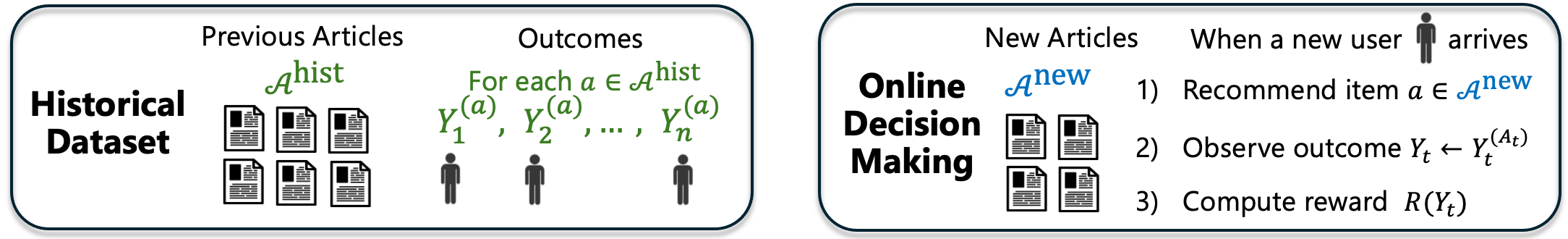
Our main insight relies on two essential structures of the problem (Figure 1). First, the agent faces recurring online decision-making problems, with a perpetual need for information gathering due to “fresh” uncertainty whenever new articles are released. This recurrence presents an opportunity to use historical data to learn how to explore effectively. Second, uncertainty on the performance of newly released articles is resolvable through exploration by repeatedly recommending an article to new users. Notably, these structures are shared by other meta-bandit problems, e.g., repeatedly learning new users’ preferences to personalize later interactions.
Algorithm: Our proposed solution proceeds in two phases. In the pre-training phase, the agent learns to model uncertainty by learning a simulator of user interactions with historical data on previously released articles. The simulator is an autoregressive sequence model that uses an article’s attributes (e.g. headline text) to predict sequences of recommendation outcomes across users for that article. To achieve near-optimal sequence prediction loss, the sequence model must implicitly learn an informed prior based on rich article headline features and how to sharpen beliefs as more outcomes are gathered.
In the online decision-making phase, the agent models its uncertainty by simulating recommendation outcomes for new users with the pretrained sequence model. When facing a new task (e.g. a new batch of articles), the agent needs to balance exploration and exploitation in sequentially selecting actions (articles to recommend). At each decision time, the agent uses the fitted simulator to autoregressively sample imagined/imputed recommendation outcomes for new users, conditioned on article features and on past outcomes. The agent then takes the action with the greatest imputed average reward.
Far from a heuristic, our approach is a principled implementation of Thompson sampling (with an implicitly learned prior), a prominent bandit algorithm with strong guarantees [68, 64, 3, 4, 63, 51, 24]. Unlike traditional implementations of Thompson sampling, our approach never performs explicit Bayesian inference regarding latent parameters, and instead relies only on predicting and generating observable quantities. This lets us train the algorithm with standard computational tools in ML.
Contributions: The connection between autoregressive sampling and Thompson sampling rests on a link between exchangeable sequence modeling and Bayesian inference that has been known since de Finetti’s seminal work [27], and has appeared in several different literatures [7, 30, 29, 36, 9, 10, 28, 55, 44]. Our derivations in Section 3 are also related to a classic view of causal inference problems as problems of missing data [39], and to Bayesian methods that impute missing outcomes by sampling from a posterior predictive distribution [62, 35]. We cement these ideas through several contributions.
-
1.
We construct a meta-bandit problem setting that both motivates and crystallizes insights connecting posterior sampling and generative sequence modeling (Section 2).
-
2.
We connect these insights to decision-making, using them to derive a new, scalable implementation of Thompson sampling (Section 3). In the process, we clarify a common misconception in recent works that make decisions using predictive uncertainty in the one-step autoregressive probabilities [49, 52, 33]. Our main algorithmic insight is that averaging autoregressively generated outcomes is a correct implementation of ”posterior sampling” of the population mean, a result from Bayesian statistics dating back to De Finetti’s seminal work [27, 22, 19, 61, 26, 18, 8].
-
3.
We provide formal links between interactive decision-making and sequence prediction, including a novel regret bound that scales with the pre-training loss of the sequence model (Section 4).
-
4.
We demonstrate that our theoretical insights bear out on a news recommendation task (Section 5). We attach a simple head to a language model that embeds article headlines and train the model end-to-end to autoregressively predict future user responses given past responses and the headline. Generation from this sequence model drives decision-making and (implicit) posterior inference.
2 Problem formulation
Online Decision-Making Problem.
Each online decision-making phase begins with new articles (actions) being released. Each article is associated with attributes ; in our experiments these represent article headlines, and successful methods need to integrate with language models that process the headline. Even with rich article headline features , the system is uncertain about how engaging articles will be to readers. The system interacts sequentially with distinct users and can adapt future recommendations based on initial user feedback. To the user, it recommends , observes an outcome , and associates with this a reward by applying a fixed, known function . The vector of outcomes could include a variety of user feedback, such as whether the user clicked on or shared the recommended article, how long the user the spent reading the article, and/or whether the user departed the website after reading.
We model recommendation potential outcomes by associating each action with potential outcomes . The observed outcome is if article is recommended to the user. This setup is standard in the bandit [43, 13] and causal inference literature [39].
We place several assumptions on the data generating process. First, we model articles as independent draws from some fixed article distribution; formally, assume the features are drawn i.i.d across articles from an unknown distribution . Conditioned on the article features , potential outcomes are drawn from an unknown distribution :
| (1) |
We assume above are sampled independently across . This simplifying assumption precludes resolving uncertainty about the effectiveness of one article by gathering feedback on a different article in the online decision-making phase. (In the pre-training phase though, our algorithm “meta-learns” across many historical articles.) Finally, we assume is exchangeable, meaning that for any permutation over , any , and any outcomes ,
| (2) |
Exchangeability means that outcomes from recommendations made to a large subset of users is likely to be representative of outcomes that would have been observed among all users.***It is not hard to formalize results of this type. For instance, for any permutation over , (3) The term is the finite population correction to the standard error of the sample mean [59, Ch 4.5]
Example 1 (Exchangeability and mixture models).
The canonical example of exchangeable sequences is mixture models, where the outcomes are i.i.d conditioned on a latent variable . That is, . The unknown latent variable represents the decision-maker’s uncertainty about an action’s performance.
Our goal is to develop an adaptive algorithm for recommending articles that maximizes the expected average reward , or equivalently, minimizes the expected per-user regret,
| (4) |
In (4) above, we calculate the gap in reward relative to a baseline that always recommends the action with best performance in the population. Similar to “Bayesian regret” in the bandit literature, the expectation integrates over the draw of the articles in , the randomness in outcomes, and any randomness in the itself. Because of the recurring nature of our problem, the expectation has a physical rather than philosophical meaning: is the long-run average regret the system would incur if were deployed across many days (and hence across many instances of the bandit task).
Pretraining Phase.
The goal of the pre-training phase is to learn a good active exploration algorithm to deploy in the online decision-making phase. We have access to a historical dataset , with action attributes and observed outcomes from previous articles (actions) , for some . We assume this dataset is drawn from the same data generating distribution as in the online decision-making phase: Across , and, is a completely random subset of size of , where .
3 Posterior Sampling via Autoregressive Generation
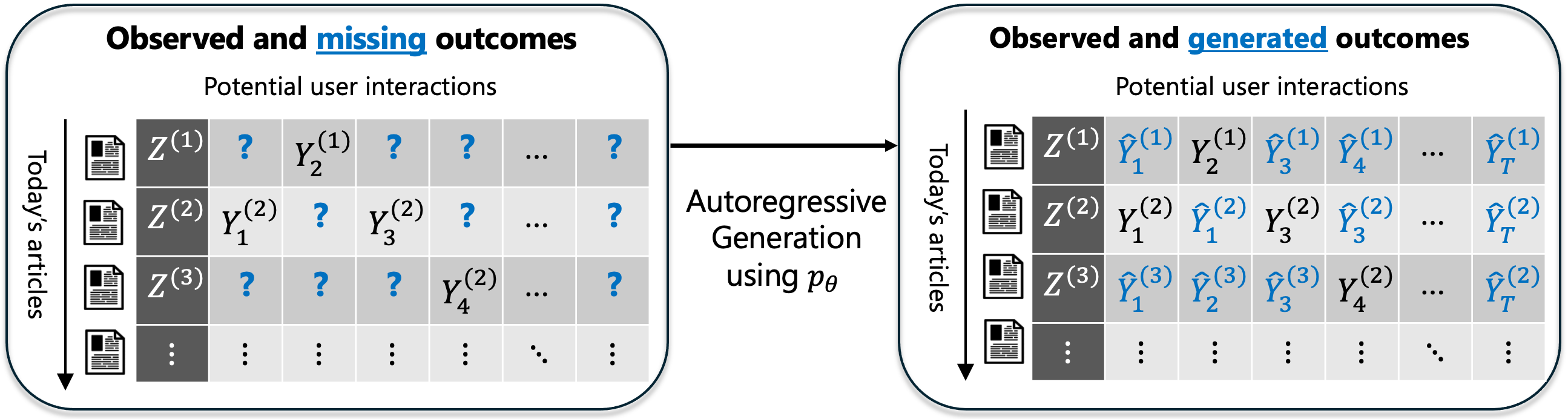
Our approach to balancing exploration and exploration in recommending newly released articles leverages rich article attributes () and historical recommendation data on articles from previous days (). The impetus of our approach is that unobserved outcome data is the source of the decision-maker’s uncertainty (see Figure 2): feedback on an article has only been gathered from a subset of users, and there is residual uncertainty in how future users would respond.
Inspired by this viewpoint, our method proceeds in two steps. First, we pretrain an autoregressive sequence model to predict successive outcomes (’s) on historical data . Then, at decision time recommendation decisions are made by imputing the missing outcomes in the potential outcomes table with hypothetical outcomes (s) generated autoregressively from the pretrained sequence model. We show a particular version of this procedure is an exact implementation of Thompson sampling (Section 3.2). Our main insight applies to general autoregressive sequence models (such as transformers), but works well empirically even with simpler sequence model architectures (Section 5).
Phase 1: Pretraining an Autoregressive Model.
We train an autoregressive sequence model , parameterized by , that can predict missing outcomes, conditioned on article (action) attributes, and limited previously observed outcomes. This will enable us to generate hypothetical completions of the potential outcome table in Figure 2. Formally, this model specifies a probability of observing outcome from the next interaction conditioned on article attributes and previous outcomes . These one-step conditional probabilities generate a probability distribution over sequences as .
Consider the sequential log-loss on the dataset when the historical data sequence lengths ,
| (5) |
In this pretraining phase, we minimize by stochastic gradient descent. In our experiments, when we use bootstrap resampling to augment the training data to ensure our model is trained to sequences of length (see details in Section 5). The bootstrap procedure also helps ensure the sequence model is approximately exchangeable, reflecting how the ’s are generated (2). Our approach to pre-training an approximate exchangeable sequence models closely mirrors recent work on neural processes [34, 41, 52, 44] and prior-data fitted networks [49], connecting also to a long tradition in Bayesian statistics and information theory [20, 5]. Our main contribution is linking the this pretrained sequence model to online decision-making, which we present next.
Phase 2: Online Decision-Making via Autoregressive Generation.
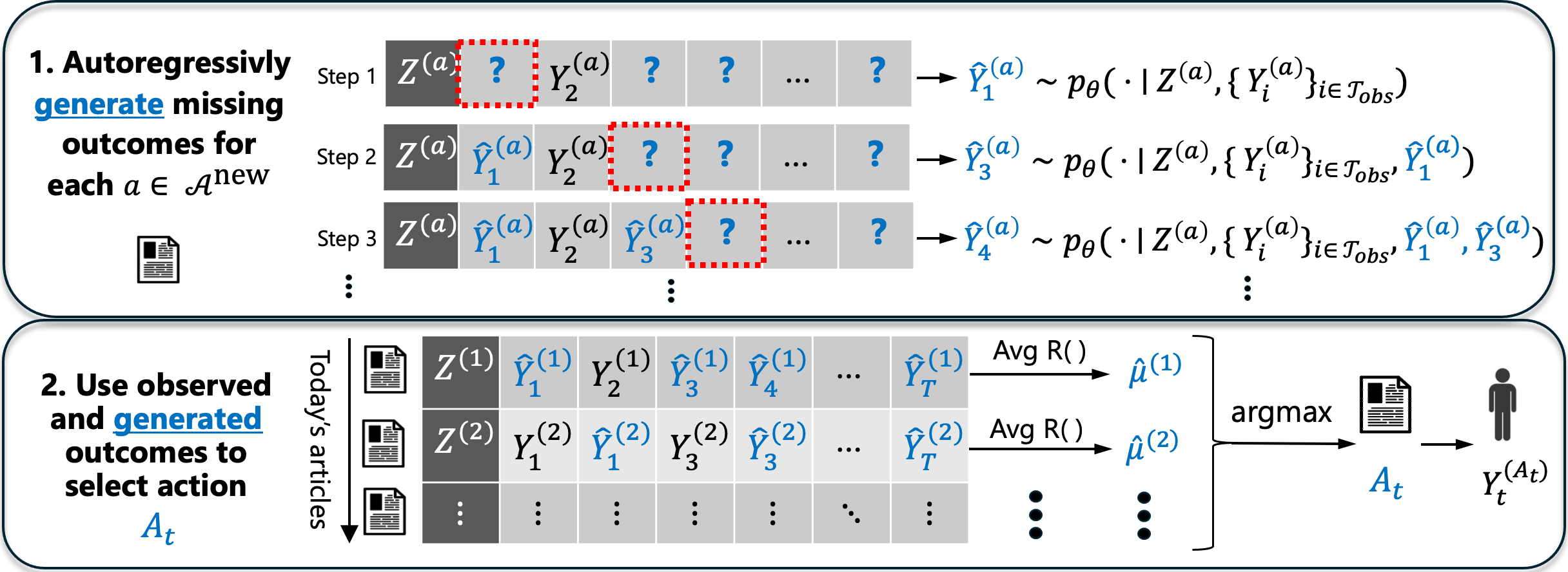
After a sequence model is trained on historical data, it is deployed and used for decision-making. No additional training of is needed. At each decision time, our algorithm uses to autoregressively generate imputed values of missing outcomes for each candidate action , as seen in Figure 3. At decision time , let denote indices of the users for which article/action has not been recommended so far. The algorithm samples (imputes) outcomes for each conditional on article attributes , as well as previously observed and generated outcomes for article . Our algorithm then uses both the observed and generated outcomes to compute an imputed mean for action :
| (6) |
Finally, the algorithm selects action . Then the real outcome is observed. The process is repeated at the next decision time. See Algorithm 2 for further details.
Through this process, actions that are optimal under some likely generation of the missing outcomes according to , have a chance of a being selected. Once no plausible sample of missing outcomes could result in an action being optimal, it is essentially written off. Good performance of the algorithm relies on the model matching the data generating process closely (formalized in Section 4).
Remark 1 (Disadvantages of Alternative Sampling Approaches).
In (6) we average the imputed rewards to form a ”posterior draw” of the population mean that reflects “epistemic” uncertainty in how users will respond on average. In forming , we average out noise (“aleatoric” uncertainty) across users. Alternative approaches of sampling from sequence models easily result in poor decision-making by over- or under-exploring. Several works [52, 49, 33] propose choosing actions using the single-step predictive uncertainty in the next outcome (no averaging across users); this reduces to random selection when outcomes across users are highly variable, as in many real-world problems (e.g. recommendation). On the other hand, averaging across many independent (non-autoregressive) draws of the next outcome reduces to the mean of the predictive distribution and results in playing the action currently believed to be best, without purposeful exploration. Similar limitations apply if one uses the most likely sequence of outcomes, instead of sampling them randomly.
Remark 2 (Including Observed Rewards in the Average).
In (6) we average over both observed rewards and imputed values of unobserved rewards. Including observed rewards helps sharpen theoretical understanding: it lets us say the algorithm is exactly a finite population (i.e. a very large group of users) version of Thompson sampling that is used in the online learning literature [14, 12]. However, it has little practical bearing on performance if is large. See Fig 6 in Appendix A.
3.1 Interpreting our Training Loss
The expected analogue of the training loss (5) (i.e., averaged over the draw of news articles) is
| (7) |
The next lemma is a standard result connecting the excess expected loss of a sequence model to its KL divergence from the true sequence model . To (nearly) minimize loss, the learner needs to closely approximate the true sequence model.
Lemma 1.
For any sequence model ,
Next we provide an example that notes connections to ideas in Bayesian statistics.
Example 1 (cont.) (Empirical Bayes).
Under the mixture model from Example 1, is called a posterior predictive distribution in Bayesian statistics. Consider the case where is a posterior predictive induced by prior hyper-parameters . For ease of exposition, imagine a setting with no ’s and a conjugate Bayesian model where and . By Bayes rule, the posterior predictive distribution is
| (8) |
For this choice of , our training criterion (5) is equivalent to that used in Empirical Bayes (Type-II maximum likelihood) to fit prior distributions to observed data [50, 15, 53]. We find that training on our sequence loss can recover the true Bayesian prior (Appendix E.2). Our pretraining procedure can be viewed as learning an approximate posterior predictive by gradient descent.
3.2 Interpreting our Decision-Making Algorithm as Posterior (Thompson) Sampling
This subsection reveals that the generated/imputed action means faithfully represent uncertainty and that PS-AR is akin to Thompson sampling (a.k.a. posterior sampling), which selects actions proportionally to the probability that they are optimal. Specifically, Lemma 2 formally shows that the imputed mean from PS-AR is a posterior sample of the mean reward , and the action selected by PS-AR is a posterior sample of the optimal action , where
| (9) |
with ties in the argmax broken by the same rule as in Algorithm 2. is the benchmark action against which regret is evaluated in (4). For simplicity, Lemma 2 is stated under the assumption that PS-AR uses the optimal sequence model . We use to denote the history up to time .
Lemma 2.
Under Algorithm 2 applied with , for all , with probability ,
Lemma 2 has a concise proof (Appendix D). Both the population mean and the best action are functions of the table of the potential outcomes . Sampling missing outcomes from their posterior distribution ensures that functions of the imputed table also follow the posterior distribution. One difference with usual presentations is that averages over a very large, but finite population of users (or rounds). We do not view this as a practically significant detail. See Appendix B.
Advantages of the Autoregressive Viewpoint.
The previous subsection suggests that PS-AR effectively implements Thompson sampling, a leading approach for balancing exploration and exploitation. We argue that the autoregressive perspective has two substantial benefits. (i) Conceptually, since the autoregressive sequence modeling approach focuses on predicting missing outcomes (i.e. ’s), this means that errors are observable and performance is measurable through a loss function like (5). In contrast, a more standard perspective on Thompson sampling requires specifying a model for latent variables and performing explicit Bayesian inference over them; for large scale problems this often involves making simplifying modeling assumptions, expensive Markov chain Monte Carlo, or heuristic posterior approximations. (ii) Autoregressive sampling also aligns with emerging engineering practice. Pretraining using the loss from (5) requires fitting a predictive model by stochastic gradient descent, as is standard practice. The PS-AR approach to uncertainty quantification can also take advantage of computational advances in autoregressive generation that are developed for other problem settings, e.g., language modeling.
4 Regret Bound
In this section we show the expected loss of the learned sequence model controls the decision-making performance of our algorithm, reducing a challenging sequential decision-making problem to a loss minimization problem. Concretely, we establish a strong regret bound for PS-AR that depends on the expected loss achieved by . Recall from (4) that denotes the regret of algorithm .
Proposition 1.
For PS-AR (Algorithm 2) applied with , which we denote as ,
Proposition 1 relies on Theorem 1, which is a result that may be of independent interest. Theorem 1 uses an information-theoretic approach to show that when the distributions and are nearly indistinguishable in a Neyman-Pearson sense (i.e., the expected log likelihood ratio is small), any function of the potential outcomes generated under vs. must also be nearly indistinguishable. Below we use to denote expectations under the distribution where the potential outcomes are generated autoregressively from , i.e., for each .
Theorem 1.
Let denote the potential outcomes table. Let be independent of . We use to denote any real-valued function of and .
The consequence of Theorem 1 is that we are able to use it to bound the deployment regret of any policy , i.e., , in terms of the regret under the simulator, , and the gap in prediction loss . Specifically,
| (10) |
Specifically, we are able to apply Theorem 1 to show (10) because the per-user regret of an algorithm as defined in (4), is simply a bounded function of all possible potential outcomes and exogenous noise if is a randomized algorithm. A formalization of this statement and proof are in Appendix D.4.
Display (10) states that the regret achieved by any algorithm under the fitted environment simulator is close to the regret will achieve when deployed in the true environment , so long as the loss achieved by is close to that of . The secondary consequence of Theorem 1 is that it characterizes the regret of Thompson sampling algorithms with a misspecified prior. To see this, pick to be Thompson sampling with a misspecified prior and pick to be the data generating distribution under the misspecified prior; then will have the typical regret bound for Thompson sampling and the second term on the RHS of (10) characterizes the penalty for having a misspecified prior. Our result can be thought of in some ways as a generalization of [66], which only applied to a “k-shot” version of Thompson sampling.
5 Experiments
We evaluate our approach in a synthetic setting and in a semi-realistic news recommendation setting. While our method applies more broadly, we focus on and , as the news dataset we build on [72] has binary click/no click outcomes. We first discuss implementation techniques:
(1) Bootstrapping Training Data. The sequence length in the training set may be smaller than the decision horizon . To ensure the learned sequence model has low prediction loss, , for longer sequences, we bootstrap the data in training by computing the loss with where are sampled with replacement from (see Appendix A for details).
(2) Truncating Generation Lengths. When the population size is large, generating missing outcomes for the entire population can be costly. To save computation, we implement a slightly modified version of PS-AR that instead generates only missing outcomes per action and averages those outcomes to form ; by (3) this is a good approximation when is relatively large. This is further supported by our simulation results where we vary (see Figure 7 in Appendix A).
5.1 Synthetic Setting: Mixture Beta-Bernoulli
Our synthetic experiments use a mixture model (Example 1) where and the prior is a mixture of two Betas and the likelihood is Bernoulli. See Appendix E.1 for more details.
Models.
We consider two sequence model variants. (i) Flexible NN is a neural network that takes and a summary of the past outcomes for action as input. (ii) Beta-Bernoulli NN, is the closed-form posterior predictive for the Beta-Bernoulli model from (8); its hyperparameters and are parameterized by neural networks that take as input.
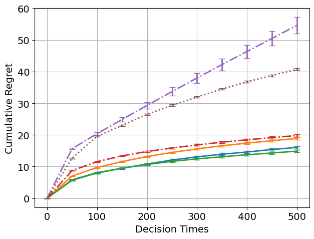
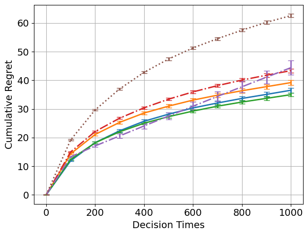
Regret: Figure 4 (Left).
PS Oracle, which implements Thompson (posterior) sampling with a prior that matches the data generating process, has the lowest regret. PS-AR Flexible NN closely matches the performance of PS Oracle. PS-AR Beta-Bernoulli NN which uses a sequence model with a misspecified, unimodal Beta prior performs similarly to PS Beta-Bernoulli (Uniform Prior) which performs exact Thompson sampling with a uniform prior. All these mentioned Thompson sampling-based algorithms outperform the UCB algorithm [1] and PS Neural Linear, Thompson sampling with a linear Gaussian bayesian model with an uninformative prior on top of learned text embeddings. See more on baseline algorithms in Appendix E.4.
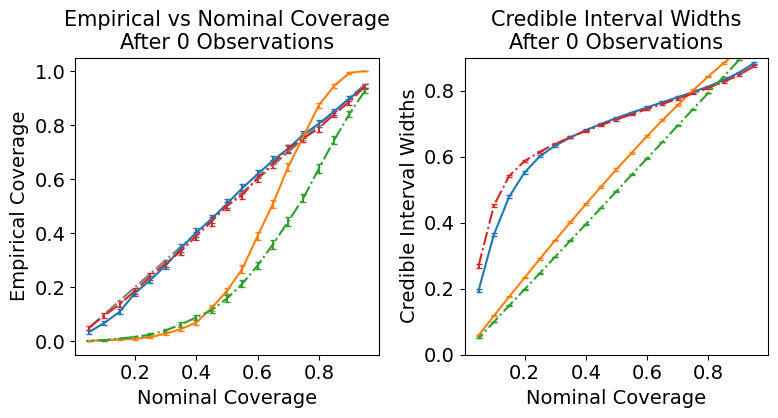
Uncertainty Quantification: Figure 4 (Right).
For 1000 actions not seen in training, we form posterior samples by autoregressively generating outcomes conditional on using . We use the percentiles of the sampled ’s to form intervals and evaluate how often the true is within these intervals; ideally, an 80% interval contains 80% of the time. The intervals generated by the Flexible NN sequence model have excellent coverage; moreover, the width of the intervals are the narrowest that have correct coverage (matching PS Oracle). In contrast, the Beta-Bernoulli NN sequence model which has a unimodal (misspecified) Beta prior has worse coverage.
5.2 News Recommendation Setting
We build a semi-realistic news recommendation task using using the MIcrosoft News Dataset (MIND) [72]. This setting demonstrates how PS-AR easily integrates with pretrained language models. Here is article headline text or news category information (e.g. ”politics” or ”sports”). Rewards are binary click/no-click outcomes. After pre-processing, the dataset has k articles (Appendix E.3).
Models
We use three model variants. (i) Flexible NN (Text) and (ii) Beta-Bernoulli NN (Text), are analogous to those from Section 5.1, but we modify them to use headline text by embedding the text using DistilBERT [65], which is fine-tuned end-to-end during pretraining. (iii) Flexible NN (Category) the final model uses category information instead of headline text.
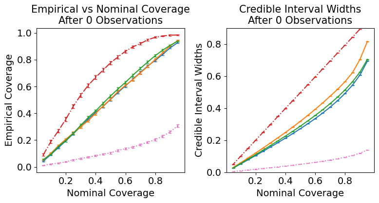
Regret and Uncertainty Quantification: Figure 5
In terms of regret, the PS-AR models that use sequence models that incorporate text features outperform all other algorithms (baselines described in Section 5.1). We use an analogous procedure as used in Section 5.1 to form uncertainty intervals for for the actions not seen in training. All PS-AR models have intervals with correct coverage, but the text-based models have slightly narrower intervals. We also compare to an ensemble of models, which we found has poor coverage. See Appendix E.3 for more details.
6 Related Work
Meta-Learning in Bandits.
There are a variety of bandit algorithms for meta-learning problems [70, 16, 42, 6]; these methods primarily focus on simpler settings (e.g. Gaussian or linear reward models). There are also deep meta-learning methods developed for recommendation systems and the cold-start problem [71, 75, 76]. These works primarily focus on more complex recommendation settings (e.g. tracking the same user over time) and not on uncertainty. In contrast, our goal is to showcase our uncertainty quantification method for decision making in a semi-realistic setting.
Reinforcement Learning (RL) with Pre-Trained Autoregressive Models.
Many recent works in RL leverage sequence models that are pretrained on a large volume of data collected by an expert policy. [45, 46] relate sampling from a model that predicts the next expert action to Thompson sampling. Other works apply goal-conditioned sampling of expert actions to improve over average expert behavior [73, 40, 17, 23, 25]; this works well in some settings but is provably sub-optimal others [11, 48]. Our work is different: we use sequence models to imagine plausible trajectories of future rewards, and use this to drive intelligent decision-making without requiring expert demonstrations.
Thompson Sampling with Deep Learning Models.
Several classes of approaches that have emerged to scale Thompson sampling to modern large scale decision-making problems that utilize neural network. The first class places a Bayesian prior on the weights of the neural network itself. These methods include those that form a Bayesian linear regression model from the last layer of a trained neural network [60, 67], as well as Bayesian neural networks [74]. A second class of approaches involves forming using an ensemble of neural networks to simulate samples from a posterior distribution [54, 47, 58]. This class also includes algorithms that build on Epinets [57, 77, 56], which attempt to retain the performance of the ensembling with lower computational cost. Notably, [57] uses sequence prediction loss to evaluate the quality of (“epistemic”) uncertainty quantification, inspiring our efforts to construct bandit algorithms using sequence models.
7 Discussion
We formulate a loss minimization problem that implicitly learns an informed prior using historical data, in order to model the posterior distribution of action rewards for decision-making. This connection enables using modern ML tools to learn rich representations to comprehend uncertainty, in an actionable way. Our formulation introduces a fresh approach to the longstanding challenge of scaling Thompson sampling to incorporate neural networks that incorporate unstructured inputs such as images and text [60]. The main ideas behind our algorithm generalize to contextual settings where user-specific contexts can be used to tailor recommendation decisions. We describe generalizing our method to this setting in Appendix C and leave a deeper dive to future work.
Limitations. We assume articles are i.i.d. between pretraining and online evaluation, and user outcomes for each action are exchangeable. Such assumptions may not be appropriate in practice, e.g., if user preferences are nonstationary. In conducting this work, we struggled to find publicly available datasets on which to evaluate our method, which led us to build our news recommendation setting. Building public benchmarks for bandit problems that require using complex inputs (e.g. text and/or images) for best performance is an important open direction. A limitation of this work is we do not provide a thorough answer as to the quality of the historical data (e.g., amount of data and/or how data was collected) necessary to ensure learning good sequence models.
References
- Abbasi-Yadkori et al. [2011] Yasin Abbasi-Yadkori, Dávid Pál, and Csaba Szepesvári. Improved algorithms for linear stochastic bandits. In Advances in Neural Information Processing Systems, pages 2312–2320, 2011.
- Achiam et al. [2023] Josh Achiam, Steven Adler, Sandhini Agarwal, Lama Ahmad, Ilge Akkaya, Florencia Leoni Aleman, Diogo Almeida, Janko Altenschmidt, Sam Altman, Shyamal Anadkat, et al. Gpt-4 technical report. arXiv preprint arXiv:2303.08774, 2023.
- Agrawal and Goyal [2012] Shipra Agrawal and Navin Goyal. Analysis of thompson sampling for the multi-armed bandit problem. In Conference on learning theory, pages 39–1. JMLR Workshop and Conference Proceedings, 2012.
- Agrawal and Goyal [2013] Shipra Agrawal and Navin Goyal. Thompson sampling for contextual bandits with linear payoffs. In International conference on machine learning, pages 127–135. PMLR, 2013.
- Barron et al. [1998] Andrew Barron, Jorma Rissanen, and Bin Yu. The minimum description length principle in coding and modeling. IEEE transactions on information theory, 44(6):2743–2760, 1998.
- Bastani et al. [2022] Hamsa Bastani, David Simchi-Levi, and Ruihao Zhu. Meta dynamic pricing: Transfer learning across experiments. Management Science, 68(3):1865–1881, 2022.
- Berti et al. [1998] Patrizia Berti, Eugenio Regazzini, and Pietro Rigo. Well calibrated, coherent forecasting systems. Theory of Probability & Its Applications, 42(1):82–102, 1998.
- Berti et al. [2004] Patrizia Berti, Luca Pratelli, and Pietro Rigo. Limit theorems for a class of identically distributed random variables. Annals of Probability, 32(3):2029 – 2052, 2004.
- Berti et al. [2021] Patrizia Berti, Emanuela Dreassi, Luca Pratelli, and Pietro Rigo. A class of models for bayesian predictive inference. Bernoulli, 27(1):702 – 726, 2021.
- Berti et al. [2022] Patrizia Berti, Emanuela Dreassi, Fabrizio Leisen, Luca Pratelli, and Pietro Rigo. Bayesian predictive inference without a prior. Statistica Sinica, 34(1), 2022.
- Brandfonbrener et al. [2022] David Brandfonbrener, Alberto Bietti, Jacob Buckman, Romain Laroche, and Joan Bruna. When does return-conditioned supervised learning work for offline reinforcement learning? Advances in Neural Information Processing Systems, 35:1542–1553, 2022.
- Bubeck and Eldan [2016] Sébastien Bubeck and Ronen Eldan. Multi-scale exploration of convex functions and bandit convex optimization. In Conference on Learning Theory, pages 583–589. PMLR, 2016.
- Bubeck et al. [2012] Sébastien Bubeck, Nicolo Cesa-Bianchi, et al. Regret analysis of stochastic and nonstochastic multi-armed bandit problems. Foundations and Trends® in Machine Learning, 5(1):1–122, 2012.
- Bubeck et al. [2015] Sébastien Bubeck, Ofer Dekel, Tomer Koren, and Yuval Peres. Bandit convex optimization:sqrtt regret in one dimension. In Conference on Learning Theory, pages 266–278. PMLR, 2015.
- Casella [1985] George Casella. An introduction to empirical bayes data analysis. The American Statistician, 39(2):83–87, 1985.
- Cella et al. [2020] Leonardo Cella, Alessandro Lazaric, and Massimiliano Pontil. Meta-learning with stochastic linear bandits. In International Conference on Machine Learning, pages 1360–1370. PMLR, 2020.
- Chen et al. [2021] Lili Chen, Kevin Lu, Aravind Rajeswaran, Kimin Lee, Aditya Grover, Misha Laskin, Pieter Abbeel, Aravind Srinivas, and Igor Mordatch. Decision transformer: Reinforcement learning via sequence modeling. In M. Ranzato, A. Beygelzimer, Y. Dauphin, P.S. Liang, and J. Wortman Vaughan, editors, Advances in Neural Information Processing Systems, volume 34, pages 15084–15097. Curran Associates, Inc., 2021. URL https://proceedings.neurips.cc/paper_files/paper/2021/file/7f489f642a0ddb10272b5c31057f0663-Paper.pdf.
- Cifarelli and Regazzini [1996] Donato Michele Cifarelli and Eugenio Regazzini. De finetti’s contribution to probability and statistics. Statistical Science, 11(4):253–282, 1996.
- Dawid [1984a] A. P. Dawid. Statistical theory: The prequential approach. Journal of the Royal Statistical Society, Series A, 147:278–292, 1984a.
- Dawid [1984b] A Philip Dawid. Present position and potential developments: Some personal views statistical theory the prequential approach. Journal of the Royal Statistical Society: Series A (General), 147(2):278–290, 1984b.
- De Finetti [1929] Bruno De Finetti. Funzione caratteristica di un fenomeno aleatorio. In Atti del Congresso Internazionale dei Matematici: Bologna del 3 al 10 de settembre di 1928, pages 179–190, 1929.
- De Finetti [1937] Bruno De Finetti. La prévision: ses lois logiques, ses sources subjectives. In Annales de l’institut Henri Poincaré, volume 7, pages 1–68, 1937.
- Ding et al. [2019] Yiming Ding, Carlos Florensa, Pieter Abbeel, and Mariano Phielipp. Goal-conditioned imitation learning. Advances in neural information processing systems, 32, 2019.
- Dong and Van Roy [2018] Shi Dong and Benjamin Van Roy. An information-theoretic analysis for thompson sampling with many actions. Advances in Neural Information Processing Systems, 31, 2018.
- Emmons et al. [2021] Scott Emmons, Benjamin Eysenbach, Ilya Kostrikov, and Sergey Levine. Rvs: What is essential for offline rl via supervised learning? arXiv preprint arXiv:2112.10751, 2021.
- Ericson [1969] William A Ericson. Subjective bayesian models in sampling finite populations. Journal of the Royal Statistical Society Series B: Statistical Methodology, 31(2):195–224, 1969.
- Finetti [1933] B de Finetti. Classi di numeri aleatori equivalenti. la legge dei grandi numeri nel caso dei numeri aleatori equivalenti. sulla legge di distribuzione dei valori in una successione di numeri aleatori equivalenti. R. Accad. Naz. Lincei, Rf S 6a, 18:107–110, 1933.
- Fong et al. [2023] Edwin Fong, Chris Holmes, and Stephen G Walker. Martingale posterior distributions. Journal of the Royal Statistical Society, Series B, 2023.
- Fortini and Petrone [2014] Sandra Fortini and Sonia Petrone. Predictive distribution (de f inetti’s view). Wiley StatsRef: Statistics Reference Online, pages 1–9, 2014.
- Fortini et al. [2000] Sandra Fortini, Lucia Ladelli, and Eugenio Regazzini. Exchangeability, predictive distributions and parametric models. Sankhyā: The Indian Journal of Statistics, Series A, pages 86–109, 2000.
- Foster and Rakhlin [2020] Dylan Foster and Alexander Rakhlin. Beyond ucb: Optimal and efficient contextual bandits with regression oracles. In International Conference on Machine Learning, pages 3199–3210. PMLR, 2020.
- Foster et al. [2020] Dylan J Foster, Alexander Rakhlin, David Simchi-Levi, and Yunzong Xu. Instance-dependent complexity of contextual bandits and reinforcement learning: A disagreement-based perspective. arXiv preprint arXiv:2010.03104, 2020.
- Garnelo et al. [2018a] Marta Garnelo, Dan Rosenbaum, Christopher Maddison, Tiago Ramalho, David Saxton, Murray Shanahan, Yee Whye Teh, Danilo Rezende, and SM Ali Eslami. Conditional neural processes. In Proceedings of the 35th International Conference on Machine Learning, pages 1704–1713. PMLR, 2018a.
- Garnelo et al. [2018b] Marta Garnelo, Jonathan Schwarz, Dan Rosenbaum, Fabio Viola, Danilo J Rezende, SM Eslami, and Yee Whye Teh. Neural processes. arXiv preprint arXiv:1807.01622, 2018b.
- Gelman et al. [2013] A. Gelman, J.B. Carlin, H.S. Stern, D.B. Dunson, A. Vehtari, and D.B. Rubin. Bayesian Data Analysis, Third Edition. Chapman & Hall/CRC Texts in Statistical Science. Taylor & Francis, 2013. ISBN 9781439840955. URL https://books.google.com/books?id=ZXL6AQAAQBAJ.
- Hahn et al. [2018] P Richard Hahn, Ryan Martin, and Stephen G Walker. On recursive bayesian predictive distributions. Journal of the American Statistical Association, 113(523):1085–1093, 2018.
- Heath and Sudderth [1976] David Heath and William Sudderth. De finetti’s theorem on exchangeable variables. The American Statistician, 30(4):188–189, 1976.
- Henighan et al. [2020] Tom Henighan, Jared Kaplan, Mor Katz, Mark Chen, Christopher Hesse, Jacob Jackson, Heewoo Jun, Tom B Brown, Prafulla Dhariwal, Scott Gray, et al. Scaling laws for autoregressive generative modeling. arXiv preprint arXiv:2010.14701, 2020.
- Imbens and Rubin [2015] Guido W. Imbens and Donald B. Rubin. Causal Inference for Statistics, Social, and Biomedical Sciences: An Introduction. Cambridge University Press, 2015.
- Janner et al. [2021] Michael Janner, Qiyang Li, and Sergey Levine. Offline reinforcement learning as one big sequence modeling problem. Advances in neural information processing systems, 34:1273–1286, 2021.
- Jha et al. [2022] Saurav Jha, Dong Gong, Xuesong Wang, Richard E Turner, and Lina Yao. The neural process family: Survey, applications and perspectives. arXiv preprint arXiv:2209.00517, 2022.
- Kveton et al. [2021] Branislav Kveton, Mikhail Konobeev, Manzil Zaheer, Chih-wei Hsu, Martin Mladenov, Craig Boutilier, and Csaba Szepesvari. Meta-thompson sampling. In International Conference on Machine Learning, pages 5884–5893. PMLR, 2021.
- Lattimore and Szepesvári [2019] Tor Lattimore and Csaba Szepesvári. Bandit algorithms. Cambridge, 2019.
- Lee et al. [2023a] Hyungi Lee, Eunggu Yun, Giung Nam, Edwin Fong, and Juho Lee. Martingale posterior neural processes, 2023a.
- Lee et al. [2023b] Jonathan Lee, Annie Xie, Aldo Pacchiano, Yash Chandak, Chelsea Finn, Ofir Nachum, and Emma Brunskill. In-context decision-making from supervised pretraining. In ICML Workshop on New Frontiers in Learning, Control, and Dynamical Systems, 2023b. URL https://openreview.net/forum?id=WIzyLD6j6E.
- Lin et al. [2024] Licong Lin, Yu Bai, and Song Mei. Transformers as decision makers: Provable in-context reinforcement learning via supervised pretraining. In The Twelfth International Conference on Learning Representations, 2024. URL https://openreview.net/forum?id=yN4Wv17ss3.
- Lu and Van Roy [2017] Xiuyuan Lu and Benjamin Van Roy. Ensemble sampling. Advances in neural information processing systems, 30, 2017.
- Malenica and Murphy [2023] Ivana Malenica and Susan Murphy. Causality in goal conditioned rl: Return to no future? In NeurIPS 2023 Workshop on Goal-Conditioned Reinforcement Learning, 2023.
- Müller et al. [2022x] Samuel Müller, Noah Hollmann, Sebastian Pineda Arango, Josif Grabocka, and Frank Hutter. Transformers can do bayesian inference. In Proceedings of the Tenth International Conference on Learning Representations, 2022x.
- Murphy [2022] Kevin P. Murphy. Probabilistic Machine Learning: An introduction. MIT Press, 2022. URL probml.ai.
- Neu et al. [2022] Gergely Neu, Iuliia Olkhovskaia, Matteo Papini, and Ludovic Schwartz. Lifting the information ratio: An information-theoretic analysis of thompson sampling for contextual bandits. Advances in Neural Information Processing Systems, 35:9486–9498, 2022.
- Nguyen and Grover [2022] Tung Nguyen and Aditya Grover. Transformer neural processes: Uncertainty-aware meta learning via sequence modeling. In Proceedings of the 39th International Conference on Machine Learning, 2022.
- Normand [1999] Sharon-Lise T Normand. Meta-analysis: formulating, evaluating, combining, and reporting. Statistics in medicine, 18(3):321–359, 1999.
- Osband et al. [2018] Ian Osband, John Aslanides, and Albin Cassirer. Randomized prior functions for deep reinforcement learning. Advances in Neural Information Processing Systems, 31, 2018.
- Osband et al. [2022] Ian Osband, Zheng Wen, Seyed Mohammad Asghari, Vikranth Dwaracherla, Xiuyuan Lu, Morteza Ibrahimi, Dieterich Lawson, Botao Hao, Brendan O’Donoghue, and Benjamin Van Roy. The neural testbed: Evaluating joint predictions. Advances in Neural Information Processing Systems, 35:12554–12565, 2022.
- Osband et al. [2023] Ian Osband, Zheng Wen, Seyed Mohammad Asghari, Vikranth Dwaracherla, Morteza Ibrahimi, Xiuyuan Lu, and Benjamin Van Roy. Approximate thompson sampling via epistemic neural networks. In Uncertainty in Artificial Intelligence, pages 1586–1595. PMLR, 2023.
- Osband et al. [2024] Ian Osband, Zheng Wen, Seyed Mohammad Asghari, Vikranth Dwaracherla, Morteza Ibrahimi, Xiuyuan Lu, and Benjamin Van Roy. Epistemic neural networks. Advances in Neural Information Processing Systems, 36, 2024.
- Qin et al. [2022] Chao Qin, Zheng Wen, Xiuyuan Lu, and Benjamin Van Roy. An analysis of ensemble sampling. In S. Koyejo, S. Mohamed, A. Agarwal, D. Belgrave, K. Cho, and A. Oh, editors, Advances in Neural Information Processing Systems, volume 35, pages 21602–21614. Curran Associates, Inc., 2022. URL https://proceedings.neurips.cc/paper_files/paper/2022/file/874f5e53d7ce44f65fbf27a7b9406983-Paper-Conference.pdf.
- Ramachandran and Tsokos [2020] Kandethody M Ramachandran and Chris P Tsokos. Mathematical statistics with applications in R. Academic Press, 2020.
- Riquelme et al. [2018] Carlos Riquelme, George Tucker, and Jasper Snoek. Deep bayesian bandits showdown: An empirical comparison of bayesian deep networks for thompson sampling. In International Conference on Learning Representations, 2018.
- Roberts [1965] Harry V Roberts. Probabilistic prediction. Journal of the American Statistical Association, 60(309):50–62, 1965.
- Rubin [1987] D. B. Rubin. Multiple Imputation for Nonresponse in Surveys. Wiley, 1987.
- Russo and Van Roy [2016] Daniel Russo and Benjamin Van Roy. An information-theoretic analysis of thompson sampling. Journal of Machine Learning Research, 17(68):1–30, 2016.
- Russo et al. [2020] Daniel Russo, Benjamin Van Roy, Abbas Kazerouni, Ian Osband, and Zheng Wen. A tutorial on thompson sampling, 2020.
- Sanh et al. [2019] Victor Sanh, Lysandre Debut, Julien Chaumond, and Thomas Wolf. Distilbert, a distilled version of bert: smaller, faster, cheaper and lighter. arXiv preprint arXiv:1910.01108, 2019.
- Simchowitz et al. [2021] Max Simchowitz, Christopher Tosh, Akshay Krishnamurthy, Daniel J Hsu, Thodoris Lykouris, Miro Dudik, and Robert E Schapire. Bayesian decision-making under misspecified priors with applications to meta-learning. Advances in Neural Information Processing Systems, 34:26382–26394, 2021.
- Snoek et al. [2015] Jasper Snoek, Oren Rippel, Kevin Swersky, Ryan Kiros, Nadathur Satish, Narayanan Sundaram, Mostofa Patwary, Mr Prabhat, and Ryan Adams. Scalable bayesian optimization using deep neural networks. In International conference on machine learning, pages 2171–2180. PMLR, 2015.
- Thompson [1933] William R Thompson. On the likelihood that one unknown probability exceeds another in view of the evidence of two samples. Biometrika, 25(3-4):285–294, 1933.
- Vaswani et al. [2017] Ashish Vaswani, Noam Shazeer, Niki Parmar, Jakob Uszkoreit, Llion Jones, Aidan N Gomez, Ł ukasz Kaiser, and Illia Polosukhin. Attention is all you need. In I. Guyon, U. Von Luxburg, S. Bengio, H. Wallach, R. Fergus, S. Vishwanathan, and R. Garnett, editors, Advances in Neural Information Processing Systems, volume 30. Curran Associates, Inc., 2017. URL https://proceedings.neurips.cc/paper_files/paper/2017/file/3f5ee243547dee91fbd053c1c4a845aa-Paper.pdf.
- Wan et al. [2023] Runzhe Wan, Lin Ge, and Rui Song. Towards scalable and robust structured bandits: A meta-learning framework. In Francisco Ruiz, Jennifer Dy, and Jan-Willem van de Meent, editors, Proceedings of The 26th International Conference on Artificial Intelligence and Statistics, volume 206 of Proceedings of Machine Learning Research, pages 1144–1173. PMLR, 25–27 Apr 2023. URL https://proceedings.mlr.press/v206/wan23a.html.
- Wang et al. [2022] Chunyang Wang, Yanmin Zhu, Haobing Liu, Tianzi Zang, Jiadi Yu, and Feilong Tang. Deep meta-learning in recommendation systems: A survey. arXiv preprint arXiv:2206.04415, 2022.
- Wu et al. [2020] Fangzhao Wu, Ying Qiao, Jiun-Hung Chen, Chuhan Wu, Tao Qi, Jianxun Lian, Danyang Liu, Xing Xie, Jianfeng Gao, Winnie Wu, et al. Mind: A large-scale dataset for news recommendation. In Proceedings of the 58th Annual Meeting of the Association for Computational Linguistics, pages 3597–3606, 2020.
- Yang et al. [2023] Sherry Yang, Ofir Nachum, Yilun Du, Jason Wei, Pieter Abbeel, and Dale Schuurmans. Foundation models for decision making: Problems, methods, and opportunities. arXiv preprint arXiv:2303.04129, 2023.
- Zhang et al. [2020] Weitong Zhang, Dongruo Zhou, Lihong Li, and Quanquan Gu. Neural thompson sampling. arXiv preprint arXiv:2010.00827, 2020.
- Zhang et al. [2021] Yin Zhang, Derek Zhiyuan Cheng, Tiansheng Yao, Xinyang Yi, Lichan Hong, and Ed H Chi. A model of two tales: Dual transfer learning framework for improved long-tail item recommendation. In Proceedings of the web conference 2021, pages 2220–2231, 2021.
- Zheng et al. [2021] Yujia Zheng, Siyi Liu, Zekun Li, and Shu Wu. Cold-start sequential recommendation via meta learner. In Proceedings of the AAAI Conference on Artificial Intelligence, volume 35, pages 4706–4713, 2021.
- Zhu and Van Roy [2023] Zheqing Zhu and Benjamin Van Roy. Scalable neural contextual bandit for recommender systems. In Proceedings of the 32nd ACM International Conference on Information and Knowledge Management, pages 3636–3646, 2023.
Appendix A Posterior Sampling via Autoregressive Generation (PS-AR) Algorithm
We present pseudo-code for the two phases of our method: pre-training (Algorithm 1) and online decision-making (Algorithm 2).
Practical Considerations for the Pre-Training Step (Algorithm 1)
-
•
In Algorithm 1 line 3, instead of bootstrapping sequences of length , for practical purposes we sometimes bootstrap samples sequences of length if training to length is very computationally expensive (we do this for our news recommendation experiments).
-
•
While we have been assuming that has sequences all of the same length , in practice, this may not always be the case. Let refer to the number of observations for article . In this case, we can easily replace with in line of Algorithm (2) (we do this for our news recommendation experiments).
Practical Considerations for the Online Step (Algorithm 2)
- •
A.1 Empirical Comparisons of PS-AR Variants
Examining Full Imputation vs Truncated Generation (Figure 6)
We empirically compare PS-AR (Algorithm 2), i.e., “full imputation”, with the computationally cheaper version of PS-AR that truncates generation to a maximum of length of (Algorithm 2 with lines 4-9 replaced with Algorithm 3). We find that both versions of PS-AR perform well in practice and that the original PS-AR (Algorithm 2) and the -truncated version (with ) have similar performance.
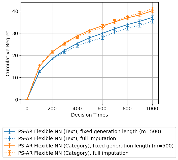
Specifically in Figure 6 we compare both versions of PS-AR on a news recommendation setting. In our experimental setup, use two versions of the pretrained autoregressive sequence model : Flexible NN (text) and Flexible NN (category) (see Appendix E.3 for more details). We run both versions of PS-AR with each of these two models. We use , , and the truncated version of PS-AR uses . We follow the procedure described Appendix E.3 in forming the regret plots: we run repetitions of each bandit algorithm and in each repetition we draw a new set of actions/articles from the validation set to represent a “new task”. Regret is calculated with respect to in Equation (9).
As discussed in Remark 2, the version of the algorithm that performs full imputation averages over both previously observed rewards and hypothetical samples of unobserved rewards when computing the imputed mean (6). The -truncated version averages solely over generated rewards. This difference does not have a practically significant impact on performance in Figure 6.
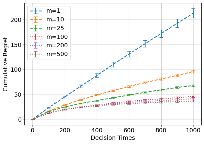
Examining Truncating Generation Length (Figure 7)
We examine the performance of our PS-AR algorithm for different generation truncation lengths (Algorithm 2 with lines 4-9 replaced with Algorithm 3). Throughout all our previous experiments we use . In Figure 7, we examine the impact of varying on the regret of the PS-AR with the Flexible NN (text) sequence model in the news recommendation setting. We follow the procedure described Appendix E.3 in forming the regret plots: we run repetitions of each bandit algorithm and in each repetition we draw a new set of actions/articles from the validation set to represent a “new task”. We find that that increasing reduces the regret of the algorithm; however, when is sufficiently large, the benefit of increasing further is negligible.
Appendix B Finite vs infinite population formulations and Thompson sampling variants
This section discusses the intimate connections between (large) finite-population formulations that were discussed in the main body of the paper and infinite-population formulations that are more common in the Bayesian bandit literature. We do this in the special case of the mixture model of Example 1.
We emphasize that from our perspective, the main advantages or disadvantages of the finite population view are conceptual. In terms of advantages: (1) the definitions do not require any explicit assumptions around mixture modeling or latent variables. and (2) The finite nature of the problem lets us visualize the procedure as in Figure 3, without abstract reference to limits across infinite sequences.
B.1 Review of Thompson sampling in infinite populations, with mixture models.
Thompson sampling is most often defined for a mixture model as in Example 1. Following that example, we consider in the subsection the canonical example of exchangeable sequences: a mixture model wherein the outcomes are i.i.d conditioned on a latent variable . That is, . The unknown latent variable represents the decision-maker’s uncertainty about an action’s performance.
The literature typically defines the “true arm means” as
The subscript highlights that this has the interpretation of a long-run average reward across an infinite population of users (or infinite set of rounds). By the law of large numbers (applied conditional on , one has
The true best arm is defined as
Randomness in the latent parameters means and are random variables whose realizations are uncertain even given the history Thompson sampling selects an action by probability matching on , defined by the property
| (11) |
Per-period Bayesian regret over periods is defined as
| (12) |
B.2 Thompson sampling in finite populations
As in the body of our paper, one can define the true mean of a finite population as
The true best arm for this finite population is defined as
As in Lemma 2, Thompson sampling selects an action by probability matching on the (finite-population) optimal action , defined by the property
| (13) |
Per-period Bayesian regret over periods is defined as
| (14) |
It is not hard to show that (14) is a more stringent notion of regret than in (12), since by definition of . Both definitions are widely used, with the more stringent finite-population version being more common in the adversarial bandit literature; see [43].
B.3 The gap between finite and infinite population formulations is small
We analyze the gap between the two formulations in the case of a mixture model. Let and recall . By a sub-Gaussian maximal inequality
To justify the last inequality, note that since the function takes values in , is subgaussian with variance proxy , conditional on (by Hoeffing’s Lemma). Since it is the average of independent sub-Gaussian random variables, is subgaussian with variance proxy , conditional on . The last step follows then from applying the subgaussian maximal inequality, conditional on .
It follows easily that the infinite population optimum is near optimal for finite populations:
Analogously, the finite population optimum is near-optimal in infinite populations:
Supported by this theory, we do not focus on the distinction between and in our developments.
B.4 Similar Insights in Empirical Results
Some empirical insight can also be gleaned from Figure 6 in Appndix B. The implementation that performs full imputation can be interpreted as Thompson sampling for a finite population. As discussed in Remark 2, averages over both past observed rewards and samples of hypothetical unobserved rewards when sampling hypthetical population means.
The implementation that performs forward generation of fixed-length does not include past observed rewards in the average. For very large , it is a direct approximation to infinite-horizon Thompson sampling. We can see in Figure 6 the these implementations have very similar performance.
Appendix C Extension to the Contextual Setting
In this section we discuss a preliminary approach to extend our algorithm to the setting with context features. In the news recommendation setting, the context features would represent user features.
Data Generating Process.
In this setting, article features are drawn independently from over . Independently of that, user contexts are discrete and drawn i.i.d. from an unknown distribution , i.e., . Then,
| (15) |
Moreover, is such that for any and any permutation over ,
where above we use to denote equality in distribution.
The historical dataset follows the same data generating process. For shorthand, we use to denote sequences of tuples. We denote the training set (for some ). For each , we assume is a completely at random subset of the tuples where and are sampled according to (15).
Phase 1: Pretraining an auto-regressive model.
We train a sequence model analogously to Algorithm 1, however replace the training loss (5) with the following loss:
| (16) |
In the contextual case, transformers are a natural choice for the sequence model architecture for .
Phase 2: Online decision-making via autoregressive generation
Online decision-making with the pre-trained sequence model can be made using Algorithm 5 below. Similar to the version without context, it generates missing outcomes.
Appendix D Theoretical Results
D.1 Proof of Lemma 1
Proof.
By the definition of the expected loss in (7), and the chain rule of KL divergence:
The final equality is the definition of the KL divergence between conditional distributions. ∎
D.2 Posterior sampling interpretation: Proof of Lemma 2
Proof.
At decision time , suppose in the history a particular action has been shown to users . For the function , one has
where are drawn according to Algorithm 2 applied with sequence model . The result that
follows immediately since are non-random conditioned on and with probability . The proof of the analogous result for is identical. ∎
D.3 Proof of Theorem 1
Proof.
Note that
-
•
(i) holds by Fact 9 in [63] (which uses Pinsker’s inequality).
-
•
(ii) holds the chain rule for Kullback Liebler Divergence.
-
•
(iii) holds because is and are independent.
-
•
(iv) and (vi) hold again because the are i.i.d. across and the chain rule for Kullback Liebler Divergence.
-
•
(vi) holds by Lemma 1.
∎
D.4 Bounding the Deployment Regret in Terms of Regret on a Simulator
Proposition 2.
For any policy ,
| (17) |
Formally, any policy can be expressed a function that maps a history and an exogenous random seed to an action as
| (18) |
The random seed allows for algorithmic randomness in action selection and is assumed to be independent of the draws of article features and potential outcomes .
The essence of the proof is to recognize that one could write a simulator that first randomly drew the environment “sample path” and the algorithm seed , and then implemented a completely deterministic sequence of operations to calculate the regret an algorithm incurs with that sample path and seed. Mathematically, the simulator is a function, (written as in the proof). We can view mis-specification of the sequence model as mis-specifying the distribution of the sample path draws used in the the simulator. We use information-theoretic tools to bound the impact this distributional change on the inputs to the simulator can have on the distribution of outputs of the simulator (e.g. regret).
Proof.
This proof will show that for any policy ,
Note for any policy , by the triangle inequality,
The remainder of the proof will focus on bounding the first term above. Let denote a draw of all article features and potential outcomes.
The absolute difference in regret can be written as
where is is a function that determines the algorithm’s regret as a function of the potential outcomes and the external seed that used to induce randomness in action actions. That is, .
D.5 Proof of Proposition 1
D.5.1 A Useful Definition
Under our data generating process is exchangeable. To prove Proposition 1, we want to view posterior sampling by auto-regressive sampling (Algorithm 2) as a proper implementation of Thompson sampling, with approximation coming solely from the incorrect use of a sequence model . To make this rigorous, we need to define a slightly different order in which potential outcomes are reveled to accommodate non-exchangeable models.
Definition 1 (An alternative outcome revelation order).
A (possibly non-exhangeable) sequence model introduces an alternative way of revealing potential outcomes. Recall, independently for each arm , nature samples arm features ; then it samples . If arm is selected at time and this is the time that arm is chosen, then is revealed. We use and .
We note that this data generating process is simply specifying the order in which outcomes from the sequence model are revealed to the decision-maker. Namely, we view as the potential outcome of the play of arm whereas the main body of the paper views as the potential outcome for the user/period. Under an exchangeable sequence models, order is irrelevant and the two data generating processes are mathematically equivalent. Note that defining the ’s is a proof technique (specifically to show Proposition 1), and not part of the model of the problem.
It will also be useful to note an alternative definition of regret under this alternative approach to revealing potential outcomes:
| (19) |
Note that since is an exchangeable sequence model, for any policy . Defining is soley to accomodate non-exchangeable sequence models.
D.5.2 A Helpful Lemma
Our proof of Proposition 1 relies on a generalization of Lemma 2 that describes precisely how Algorithm 2 is exactly Thompson Sampling (i.e., probability matching) when is not exchangeable.
Lemma 3.
Proof.
We use the notation of Definition 1. Let denote the number of times arm was played up to and including period . Then, the observation at time is
For the function , one has
where represent the generated outcomes drawn according to Algorithm 2 applied with sequence model . Property (20) follows immediately since are non-random conditioned on the history and
with probability . The proof of (21) is identical.
∎
D.5.3 Main Proof
The following proof of Proposition 1 is largely review of an information-theoretic analysis of Thompson sampling due to [63]. It was observed by [14, 12] that this analysis applied without modification to analyze regret with respect to the best fixed action () even in nonstationary environments (e.g. non-exchangeable models as in Definition 1.)
Proof.
This proof will show that for any sequence model ,
Note that by Theorem 1, we can show that
| (22) |
Specifically the argument to show (22) above is equivalent to that used to prove Proposition 2—all that needs to be done is to replace all ’s with ’s and replace all ’s with ’s in the proof.
Note that since is an exchangeable model (2), for any permutation over elements,
The above implies that the average regret achieved by a policy under the two different approaches of revealing potential outcomes are equivalent, i.e.,
Thus, combined with (22), we have that
All that remains is to bound .
Bounding .
We bound by combining the probability matching result of Lemma 2 with Thompson sampling regret bound techniques from Russo and Van Roy [63]. By the proof of Proposition 1 of [63] (which is general and applies to all algorithms ),
where refers to the conditional Shannon entropy of given under the data generating process defined by , and is a constant upper bound on the “information ratio” such that
Above we use where denotes the number of times arm was played up to and including period . Above we use to denote that expectations are conditioned on the history and to denote the mutual information between and conditional evaluated under a base measure () that conditions on . (Recall that the history also includes the information in ).
The proof of Proposition 5 of [63] shows that one can choose w.p. . As observed in [14, 12], this proof relies only on the probability matching property in Lemma 3 and hence applies in our setting.
Combining our results implies
so the result follows by the law of iterated expectations. ∎
Appendix E Experiment Details
In this appendix we discuss synthetic experiments in Section E.1, news article recommendation experiments in Section E.3, and bandit algorithms in Section E.4.
E.1 Synthetic Experiments: Mixture Beta-Bernoulli
Data generating process
In this setting, we use article attributes be where . We sample by first sampling from a mixture:
Then, outcomes are sampled as .
Here, corresponds to the success rate in the data generating process, in contrast to in the main text of the paper, which corresponds to the mean (or success rate) in the finite-sample population of size . Note that converges to as goes to infinity.
Training and Validation Datasets
The training and validation datasets contain 2500 and 1000 articles each, respectively. During training (Algorithm 1), we use . Hyperparameters and early stopping epochs are chosen using the validation dataset.
Additional model and training details
-
•
Flexible NN. This model implements the autoregressive model as a neural network that takes as input the action/article attribute (a vector in ) and summary statistics of observations for this action, and outputs a value (probability) in . The summary statistic we use is simple because outcomes are binary; specifically it consistes of a tuple with the mean of outcomes from action , and the reciprocal of 1 plus the total number of outcome observations for action , i.e. , where . (In practice, we found that repeating the summary tuple input improved performance, so the model took as input vectors in 22 which consisted of a -dimensional and copies of the sufficient statistic tuple). Note that this entire could alternatively be implemented as a transformer.
The MLP we use has three linear layers, each of width 50. After the first and second linear layers, we apply a ReLU activation. After the last linear layer, we apply a sigmoid function, so that the output is in . The models are trained for 1000 epochs with learning rate 0.001, batch size 500, and weight decay 0.01 using the AdamW optimizer.
-
•
Beta-Bernoulli NN. This is a sequential model that is the (closed-form) posterior predictive for a Beta-Bernoulli. The prior parameters for the Beta distribution, and , are each parameterized by separate neural network MLP models that take in .
The MLPs we use has three linear layers, each of width 50. After the first and second linear layers, we apply ReLU activations. After the last linear layer, we also apply a ReLU activation, so that the final output is in . We initialize weights so that the bias term for both and to 1, so that we avoid starting with Beta parameters of value 0, as Beta parameters need to be positive. The models are trained for 1000 epochs with learning rate 0.001, batch size 500, and weight decay 0.01 using the AdamW optimizer.
Additional details on Figure 4
In our uncertainty quantification plots Figure 4 (right), we evaluate over all actions in the validation set. We form samples of for each action in the validation set using Algorithm 3 with . To generate posterior samples for Beta-Bernoulli NN, we use the closed-form posterior (i.e., ).
In our regret plots Figure 4 (left), we run runs. In each run we randomly choose actions randomly with replacement from the validation set, and all algorithms are evaluated on these same sampled actions in each run. Regret is calculated relative to from the data generating process.
E.2 Additional Synthetic Experiments: Recovering the True Prior / Empirical Bayes
We discussed connections between our pretraining procedure and empirical Bayes below (8) (Example 1 continued). Here, we demonstrate in practice an setting where we perform “empirical Bayes” using our pretraining procedure (Algorithm 1). We find that we recover the true prior fairly well.
Data generation
We use a synthetic Beta-Binomial data generating process. We consider one-dimensional action features . We then sample from a Beta distribution, where
| (23) |
Then, . We use . We use a training dataset of size 25,000 actions and a validation set of size 10,000 actions; both datasets have observation sequences of length .
Autoregressive model
We use which matches the posterior predictive of a Beta-Bernoulli distribution, akin to (8). To accomodate features, we parameterize the prior hyperparameters: (we follow the procedure described in Appendix E.1 for Beta-Bernoulli NN). The neural network model architecture used in and the training procedure are also the same as described for Beta-Bernoulli NN in Appendix E.1 (except that the MLP widths are 100).
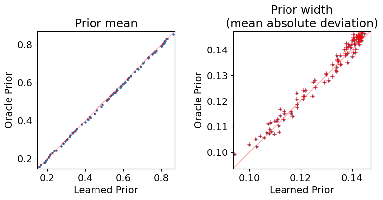
Recovering the Prior: Figure 8
We show in Figure 8 that through our pretraining procedure Algorithm 1 with our particular choice of model class, that we (approximately) recover the true prior. We show this by comparing means and standard deviations of samples from our learned prior (using ) vs. the true prior (according to the data generating process), for different draws of . In the scatter plots, each point corresponds to one .
Specifically, in these plots we use actions sampled uniformly from the validation set. For each of these actions we form samples of using Algorithm 3 using our learned model. We also form samples from the true data generating prior (23) for each of the actions. Then for each action, we compute the mean and standard deviations of the samples on the “prior” samples from ; we also compute the mean and standard deviations of the samples from the true prior. We then plot these in a scatter plot; for each action, we have the prior mean according to vs the prior mean according to the data generating process—this forms one point on the scatter plot. A similar procedure is plotted on the right. There, instead of computing the mean of the prior samples, we compute a measure of the spread of the prior samples: let be the prior samples. Let . Then we compute the mean absolute deviation for this set of prior samples.
E.3 News Recommendation Experiment Details
Additional data details
The training and validation datasets contain 9122 and 2280 distinct actions/articles each, respectively. During training, we use As in Appendix E.1, hyperparameters and early stopping epochs are chosen using the validation dataset.
We now discuss the news data preprocessing process. This dataset is free to download for research purposes at https://msnews.github.io/. It is under a Microsoft Research License at https://github.com/msnews/MIND/blob/master/MSR%20License_Data.pdf, which we comply with. The terms of use are at https://www.microsoft.com/en-us/legal/terms-of-use.
Our preprocessing procedure is as follows:
-
1.
Collect all articles from the MIND “large” dataset (training split only) [72].
-
2.
Remove any article with fewer than 100 total impressions.
-
3.
Normalize the success probabilities to be centered around 0.5 in a way that preserves the ranking of . We do this transformation to speed up the learning procedure (since it requires more data to learn small true Bernoulli success probabilities accurately). We leave simulations without this transformation to future work.
Our transformation procedures as follows: Let be the original empirical success probabilities (average click rate). We use to denote all articles in the MIND large dataset. The new success probabilities are defined as follows for each :
Above, and . See Figure 9 for comparison of the success probabilities (click rates) before and after the transformation.
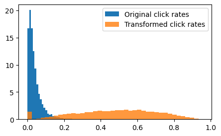
Figure 9: Original and transformed click rates. Note the spike at 0 for transformed click rates: only click rates that were not 0 or 1 are transformed. -
4.
Randomly select 20% of the remaining articles to be in the validation set; the rest are in the training set.
Additional model details
-
•
Flexible NN (text). This model very similar to the Flexible NN model in Appendix E.1, with the exception that in place of a two-dimensional , the MLP head of the neural network from before is fed as input a DistilBERT [65] embedding of text data .
Also, the MLP linear layers have width 100 instead of 50, and the sufficient statistics are repated 100 times instead of 10 times. All other architecture details are the same.
The model is trained for 500 epochs with learning rate 1e-5 on MLP heads, 1e-8 on the DistilBERT weights, batch size 500, and weight decay 0.01 using the AdamW optimizer.
-
•
Beta-Bernoulli NN (text). This is very similar to the Beta-Bernoulli posterior predictive sequence model in Appendix E.1, with the exception that in place of a two-dimensional , the MLP head of the neural network from before is fed as input a DistilBERT [65] embedding of text data . On top of the one DistilBERT embedding are two separate MLP heads for and , which are trained together. Also, the MLP linear layers have width 100 instead of 50, and the sufficient statistics are repated 100 times instead of 10 times. All other architecture details are the same.
The model is trained for 500 epochs with learning rate 1e-5 on MLP heads, 1e-8 on the DistilBERT weights, batch size 500, and weight decay 0.01 using the AdamW optimizer.
-
•
Flexible NN (category). This is very similar to the flexible neural network model in Appendix E.1, but it uses a one-hot new category vector for instead of a two-dimensional . The model architecture and training parameters are also the same.
-
•
DistilBERT. Our two text models use DistilBERT [65] from https://huggingface.co/distilbert/distilbert-base-uncased. It has an apache-2.0 license, with license and terms of use at https://huggingface.co/datasets/choosealicense/licenses/blob/main/markdown/apache-2.0.md.
Additional details on Figure 5
In our uncertainty quantification plots Figure 5 (right), we evaluate over all articles/actions in the validation set. For our Flexible NN model, we form samples of for each action in the validation set using Algorithm 3 with . For our Beta-Bernoulli NN model we use samples from the closed-form posterior.
In our regret plots Figure 5 (left), we run runs. In each run we randomly choose actions randomly with replacement from the validation set, and all algorithms are evaluated on these same sampled actions in each run. Regret is calculated relative to as described above.
Ensemble
We describe the ensembling approach used in the uncertainty quantification plots in Figure 5 (right). To construct ensembles, we first train a DistilBERT model with an MLP head (MLP width 100, 3 layers, batch size 100, 500 epochs, learning rate 1e-5 on the head and 1e-8 on DistilBERT, weight decay 0.01, AdamW optimizer) to predict , using action/article features (headlines). Then, we freeze the DistilBERT weights, and train 50 MLP heads from scratch with random initialization and bootstrapped training data to create the ensemble (50 epochs, fixed DistilBERT embedding; other params the same as before). We include a “randomized prior” variant that initializes each neural network model in the ensemble in a particular way to encourage diversity [54].
E.4 Bandit Algorithms
We compare our method with several baseline bandit methods.
PS Beta Bernoulli (Uniform Prior)
We model success rate and potential outcomes using a conjgate Beta-Bernoulli model:
| (24) | ||||
| (25) |
We also use reward mappings . In our experiments, we use Beta-Bernoulli with a uniform prior, so . Note that unlike the Beta-Bernoulli NN, the prior here does not depend on action attributes .
Online decision-making uses Thompson sampling, as described in in Algorithm 6.
PS Neural Linear
We implement a variation of “neural linear” as in Riquelme et al. [60], Snoek et al. [67]. Our problem setting differs from theirs. Their bandit setting has a small, fixed number of actions without features , and contexts . They also do not have a large historical dataset that can be used for pretraining, and the algorithm must make better decisions solely on the data (rewards) that it gathers through online decision-making.
We create an adapted version of “neural linear” for our setting. First pretrain a (non-sequential) prediction model using that takes as input the text and outputs a prediction for . The architecture of this model is that it takes the input text puts it through a DistilBERT model, and puts the output of DistilBERT through an MLP with (width 100, 3 layers). This model has been trained with learning rate 1e-5, batch size 500, and weight decay 0.01 using the AdamW optimizer. We use to refer to the last layer output of article ’s headline text.
Then we model clicks using a Bayesian linear regression, across actions: for a fixed ,
| (26) | ||||
| (27) | ||||
| (28) |
where denotes a vector of 0’s of size 768, and denotes an identity matrix of size .
The bandit algorithm consists of 3 rounds of round-robin (choosing each action in sequence) as in Riquelme et al. [60], and then afterwards, it uses Thompson sampling with the model above, using the posterior of conditioned on observations across all actions that have been selected. In our experiments we set . We also try (omitted) but this change does not make a meaningful difference in regret.
One reason why this version of neural linear does not perform very well compared to other bandit methods in our experiments is that by modeling actions together in this way, it is not possible to estimate the click rate for an action in a way that approaches 0 error as the number of observations for that action increases, unlike other methods (e.g. our PS-AR methods, as well as PS Beta Binomial, UCB, and SquareCB).
UCB
For UCB we use the multi-arm bandit algorithm described in Section 6 of [1]. We set the failure probability and use sub-Gaussian parameter (since we have binary rewards).
SquareCB
In these experiments, we use the flexible neural network with text attributes, but instead of using Thompson sampling, we use SquareCB [31], which is a bandit algorithm that uses a regression oracle to predict the value of each action. Note that our setting differs from the setting of SquareCB [31], as SquareCB assumes that the prediction model for action value is being learned online, while our prediction model has been pretrained on historical data and is not learned online.
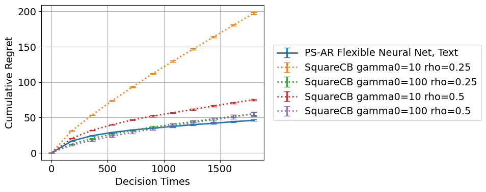
For setting the learning rate in SquareCB [31], we follow Foster et al. [32] and consider a time-varying learning rate , where (a subset of those suggested in Foster et al. [32]), and are hyperparameters. While some hyperparameter combinations for SquareCB perform almost as well PS-AR Flexible NN (Text), we remark that there is no principled approach to choosing the learning rate provided in existing works (besides grid search by deploying the algorithm many times).
E.5 Compute resources
Unless otherwise specified, computational experiments were run on an internal CPU cluster at Columbia GSB, where for any individual run we request at most 50GB of memory, and each individual training run takes at most an hour or two.
We train on a GPU only for text models that fine-tune DistilBERT, which applies to learning sequence models for the MIND news setting (Section 5.2, Appendix E.3). In these cases, each run uses a single NVIDIA A40 GPU, and a single training run of the slowest variant Flexible NN (text) takes about 16 hours to complete. We ran hyperparameter sweeps and tried several architecture variations, so we estimate the total compute to be an order of magnitude or two larger than that of a single run. Note that we use the CPU cluster for e.g. ensembling, where we freeze the DistilBERT part of the model and train MLP heads with random initializations on bootstrap-resampled subsets of the data.
Appendix F When is an Autoregressive Sequence Model a Valid Posterior Predictive?
In Algorithm 1, we learn an autoregressive model to use in place of a posterior predictive in Algorithm 2. We make this connection in Section 4 and establish a regret bound for Algorithm 2 that holds whenever has low loss.
In this section, we address the following question: When is a valid posterior predictive, for some underlying Bayesian model?
In order for an autoregressive generative sequence model to be a valid posterior predictive distribution, the sequence model to be infinitely exchangeable. We say that a sequence model is an infinitely exchangeable sequence model if it generates infinitely exchangeable random variables (Definition 2).
Definition 2 (Exchangeablity).
A sequence of random variables is exchangeable if for any permutation , the following are equal in distribution:
An infinite sequence of random variables is infinitely exchangeable if any finite subset is exchangeable.
Practically, this means that the models we train need to be invariant to the order in which previous outcomes are fed into the model. The key insight behind why infinitely exchangeable sequence models are valid posterior predictives is De Finetti’s Representation Theorem (Theorem 2 below). We state this Theorem for binary outcomes for simplicity [21, 37], but it generalizes to real-valued outcomes [22].
Theorem 2 (De Finetti’s Representation Theorem for Binary Outcomes).
If a sequence of binary random variables is infinitely exchangeable, then there exists a unique distribution on such that for some ,
The implication of Theorem 2 is that any infinitely exchangeable sequence of binary random variables can equivalently be described as being generated by a particular Bayesian model with a Bernoulli likelihood. Above, is a latent success probability that is drawn from some prior distribution .
In practice note that our bootstrap training procedure in Algorithm 1 helps ensure our sequence model is approximately exchangeable.