Clustering-Based Validation Splits for Domain Generalisation

Abstract

This paper considers the problem of model selection under domain shift. In this setting, it is proposed that a high maximum mean discrepancy (MMD) between the training and validation sets increases the generalisability of selected models. A data splitting algorithm based on kernel k-means clustering, which maximises this objective, is presented. The algorithm leverages linear programming to control the size, label, and (optionally) group distributions of the splits, and comes with convergence guarantees. The technique consistently outperforms alternative splitting strategies across a range of datasets and training algorithms, for both domain generalisation (DG) and unsupervised domain adaptation (UDA) tasks. Analysis also shows the MMD between the training and validation sets to be strongly rank-correlated ($\rho=0.63$) with test domain accuracy, further substantiating the validity of this approach.

1 Introduction

The ability for models to maintain high performance on data lying outside their training distribution, known as domain generalisation (DG), is crucial to the widespread deployment of AI. Although extensive research has been conducted towards developing more generalisable training algorithms [1], significantly less focus has been given to increasing the robustness of the model selection process, despite being as integral a part of the learning problem, and indeed, just as susceptible to distribution shifts, as the fitting of the model itself.

As with model parameters, hyperparameter choices based on in-distribution (ID) performance may not be optimal on an out-of-distribution (OOD) test domain. As such, OOD validation sets (distinct from both the training and test sets) are commonly employed, normally created through the use of additional metadata (e.g., domain labels). Empirical evidence supports the assumption that this encourages the selection of more generalisable hyperparameters [2]. In this paper, it is proposed that the validation set should indeed be maximally domain shifted from the training set, given some quantitative distance measure such as the maximum mean discrepancy (MMD), while still retaining a relevant distribution. It is proposed that this would further encourage the selection of robust hyperparameters.

To this end, it is noted that the kernel k-means clustering problem can be re-posed as the problem of maximising the empirical MMD between clusters (weighted by cluster size). In light of this, it is proposed to perform a validation split based on kernel k-means, and a modified clustering algorithm is presented for this purpose. Specifically, constraints are introduced to the cluster assignment step to control the holdout fraction (i.e., the cluster sizes), and to preserve class and (optionally) domain/group distributions; this is then formulated and solved as a linear program, providing convergence guarantees not present in prior work. In addition, the Nyström method for low-rank approximation is employed to make the algorithm tractable for large datasets.

The proposed method provides a model selection strategy based on OOD performance that does not require additional metadata, which is not always available. It is also argued that the method is able to capture more nuances in real-world data than can be described by a single domain variable. For example, in tumour identification, domain shifts can be caused by variations in sample preparation methods or patient populations. Or, in wildlife monitoring (both acoustic and visual), these can be due to differences in environmental or weather conditions, data collection equipment, or new unseen events [2]. However, all this information is unlikely to be described in the available meta-data, which may only state the hospital of origin or the recording location, respectively. In such cases, splitting the data along lines closer to the underlying cause of the shift, as determined by the clustering algorithm, rather than a more loosely correlated proxy, may permit a more informed model selection which can result in hyperparameters better suited to the nature of the shift.

Clustering the development data can also serve as a natural way of disentangling spurious cues and ensuring these are not carried over to the validation set. To illustrate this, consider the Coloured MNIST (CMNIST) dataset [3], in which a digit’s colour is spuriously correlated with its label. Applying vanilla k-means here would perfectly separate the two colour groups. The colour shortcut would then be absent from the validation set, meaning the model selection can be based on recognition of the intended attribute (the digit) instead. Of course, due to CMNIST’s unrealistically simple structure, it is trivial for vanilla clustering to separate the spurious attribute here. Moreover, the validation set would then closely align with the test distribution in this case, which is unlikely to occur in real-world data. Therefore, this dataset, along with any others comprising synthetically varying subpopulations of a spurious variable (CelebA [4, 5], Waterbirds [4], Spawrious [6], etc.), are not considered valid benchmarks to test this method on.

In summary, this paper contributes the following:

• Description of a constrained clustering algorithm based on kernel k-means which can be used to perform a validation split in applications expected to involve domain shifts.

• Comparison of this approach with existing validation strategies for a range of datasets and algorithms, in both DG and UDA settings.

• Analysis of the relationship between test domain accuracy and the MMD between the training and validation sets.

1.1 Relation to existing work

[1] reviewed 3 criteria for model selection in a DG setting: ID accuracy (on a randomly held-out subset of each training domain); OOD accuracy on an additional domain held-out using metadata (referred to as leave-one-domain-out); and test-distribution accuracy on a held-out subset of the test domain (referred to as the oracle criterion), which can be used to provide an upper bound on performance. Where the validation set comprises multiple domains, these authors take the average accuracy over these domains, although it has been argued that considering only the worst-performing domain provides a more robust indicator of generalisability [4, 7].

In a link to the latter, clustering-based splits can also be viewed as a measure of worst-case performance – where the worst-case performance of a given set of hyperparameters is assumed to correspond to the validation accuracy when the MMD between the training and validation sets is maximised.

In addition to validation accuracy, it has been suggested that a model’s stability to distribution shifts should also be explicitly considered. Prior work has quantified stability in terms of the expected calibration error (the average deviation between accuracy and confidence) [8]; the MMD between features from different domains [9]; or the average variation of each feature between domains [10].

It has also been proposed to induce a domain shift between the training and validation sets by performing mix-up augmentation on the held-out data [11]. This also links to a range of general robustness benchmarks, where the evaluation sets have been subjected to various synthetic transformations. For example, visual corruptions and perturbations [12], stylisation [13], the addition of spurious cues [14], and adversarial filtration [15] have all been employed; a more complete review of this approach is given in [2].

Non-random data splits have previously been used to produce domain-shifted evaluation sets, but no prior work has investigated the benefits this may bring to hyperparameter tuning. [16] proposed an adversarial split which heuristically aims to maximise the Wasserstein distance between clusters, but no attempt was made to control label distribution. Similarly, [17] proposed a split based on constrained k-means clustering, with constraints on cluster size and label distribution imposed using a greedy algorithm. However, since greedy assignments can be sub-optimal, the clustering objective is not guaranteed to reduce at every iteration. Consequently, convergence of this algorithm is not guaranteed. The current paper develops on this by formulating the constrained assignment as a linear program. As this can be solved globally, the clustering objective must reduce (unless it is already at a local minimum), guaranteeing convergence.

1.2 Preliminaries and notation

Let $S=\{(x_{1},y_{1},d_{1}),\ldots,(x_{n},y_{n},d_{n})\}$ be the development set consisting of input-label-domain triplets over $\mathcal{X}\times\mathcal{Y}\times\mathcal{D}^{S}$. Similarly, let $E$ be the evaluation set over $\mathcal{X}\times\mathcal{Y}\times\mathcal{D}^{E}$, where $\mathcal{D}^{S}\cap\mathcal{D}^{E}=\emptyset$ (i.e., the development and evaluation domains are disjoint). For ease of notation, subscripts are used on sets to simplify set-builder notation, in two ways. Firstly, “slices” of a set are denoted using capitals, for example:

$$S_{X}=\{x:(x,y,d)\in S\}$$

$$S_{YD}=\{(y,d):(x,y,d)\in S\}.$$

Additionally, a predicate can be specified to restrict the set to samples satisfying a condition. For example, to denote only inputs associated with a specific class $y^{\prime}$:

$$S_{X,y=y^{\prime}}=\{x:(x,y,d)\in S\land y=y^{\prime}\}.$$

In short, the goal of DG is to use $S$ to produce a model $\theta:\mathcal{X\rightarrow Y}$ that performs well on $E$. $\theta$ comprises a featuriser $\theta_{F}:\mathcal{X\rightarrow F}$ and label classifier $\theta_{C}:\mathcal{F\rightarrow Y}$, such that $\theta=\theta_{C}\circ\theta_{F}$. In order to tune hyperparameters, $S$ must be partitioned into training and validation sets, $T$ and $V$ respectively. A number of models are trained on $T$ using different hyperparameters; the “best” model, according to some criterion on $V$, is then selected and evaluated on $E$.

$T$ and $V$ should be of sizes determined by a user-defined holdout fraction $h$ satisfying $0<h<1$, and have equivalent class distributions. This can be achieved by constraining the size of each label group in $V$ to $h$ times the size of the corresponding group in $S$:

$$\left|V_{y=g}\right|=h\left|S_{y=g}\right|,\ \ \forall g\in\mathcal{Y}.$$ (1)

It may also be necessary or desirable to control domain distributions – for example, certain training algorithms may require the domains in $T$ to be uniformly represented to avoid overfitting. In this case, the constraints should be taken over all $(y,d)$ pairs instead:

$$\left|V_{(y,d)=g}\right|=h\left|S_{(y,d)=g}\right|,\ \ \forall g\in\mathcal{Y\times D}.$$ (2)

For the remainder of this section, the latter set of constraints (2) are assumed, although (1) can easily be substituted if desired (as this would further increase the MMD between $T_{X}$ and $V_{X}$), or if domain labels are unavailable.

It is also proposed that $V$ should be maximally domain shifted with respect to $T$. It is proposed to measure this as the MMD between the distributions of feature sets $\theta_{F}\left[T_{X}\right]$ and $\theta_{F}\left[V_{X}\right]$, where $\theta_{F}[\cdot]$ denotes the image under $\theta_{F}$.

Assume $\theta_{F}\left[T_{X}\right]$ and $\theta_{F}\left[V_{X}\right]$ are samples from distributions $\mathbb{P}_{T},\,\mathbb{P}_{V}$ over $\mathcal{F}$. A positive-definite kernel $\kappa\ \mathcal{:F\times F}\rightarrow\mathbb{R}$ induces a unique reproducing kernel Hilbert space (RKHS) $\mathcal{H}$ on $\mathcal{F}$, along with a mapping $\phi\mathcal{\ :F\rightarrow H}$. The empirical mean map of $\mathbb{P}_{T}$ (and analogously for $\mathbb{P}_{V}$) in $\mathcal{H}$ is given by

$$\mu_{\mathbb{P}_{T}}=\frac{1}{\left|T_{X}\right|}\sum_{f\in\theta_{F}\left[T_{X}\right]}{\phi(f)}.$$

The MMD can then be estimated as the distance between means of samples embedded in $\mathcal{H}$:

$$\text{MMD}\left(\mathbb{P}_{T},\mathbb{P}_{V}\right)=\left\|\mu_{\mathbb{P}_{T}}-\mu_{\mathbb{P}_{V}}\right\|_{\mathcal{H}}.$$

1.3 Problem formulation

The partitioning problem can now be formulated as

$$\arg{\max_{T,V}\left\|\mu_{\mathbb{P}_{T}}-\mu_{\mathbb{P}_{V}}\right\|_{\mathcal{H}}}$$ (3)

subject to (2).

This is equivalent to minimising the standard kernel k-means objective, subject to the same constraint:

$$\arg{\min_{T,V}{\sum_{\begin{subarray}{c}J\in\left\{T,V\right\}\\ f\in\theta_{F}\left[J_{X}\right]\end{subarray}}\left\|\phi(f)-\mu_{\mathbb{P}_{J}}\right\|_{\mathcal{H}}^{2}}}$$ (4)

subject to (2).

Proof.

The relation can be derived by applying the law of total variance. The objective in (4) is to minimise the within-cluster sum of squared deviations from each centroid (in feature space). As the total variance is constant, this is equal to maximising the between-cluster sum of squares from each cluster centroid to the grand one, weighted by cluster size:

$$\arg{\max_{T,V}{\sum_{J\in\{T,V\}}{\left|J_{X}\right|\left\|\mu_{\mathbb{P}_{J}}-\mu_{\mathbb{P}_{S}}\right\|_{\mathcal{H}}^{2}}}}.$$

Since the cluster sizes are fixed by the constraint, the $\left|J_{X}\right|$ term can be dropped from the objective function. With only two centroids, this is then equivalent to directly maximising the distance between them, which is the formulation in (3). ∎

(4) can be solved by iterating between 2 steps until convergence:

1. The update (maximisation) step computes the distance matrix $D\in\mathbb{R}^{n\times 2}$ from each point to each centroid using the kernel trick. For large datasets, the Nyström method [18] is employed to reduce the complexity of the kernel computations from $O(n^{2})$ to $O(qn)$, by computing only a randomly selected submatrix of the full kernel, of size $q\times n$.

2. The constrained assignment (expectation) step computes the one-hot cluster assignment matrix $U\in\left\{0,1\right\}^{n\times 2}$ that assigns each point to exactly one of the two centroids.

As in the standard Lloyd’s algorithm, convergence to a local minimum is guaranteed as each step individually optimises (4). $U$ is the solution to the binary linear program (LP):

$$\mathrm{arg}\,\min_{U} \,{\operatorname{Tr}\left(U^{T}D\right)}$$ (5)

subject to

$$U_{ij}\in\left\{0,1\right\}\ \operatorname{for}i\in\{1,\ldots,n\};\ j\in\left\{1,2\right\}$$ (6)

$$\sum_{j}U_{ij}=1\ \operatorname{for}i\in\{1,\ldots,n\}$$ (7)

$$\sum_{i|\left(y_{i},d_{i}\right)=g}U_{ij}=\operatorname{round}\left(h\left|S_{(y,d)=g}\right|\right)\ \operatorname{for}g\in\mathcal{Y\times D};\ j=1\ \text{or}\ 2.$$ (8)

(7) ensures that each point is assigned to only one cluster. The disjunctive constraint (8) enforces (2), and indicates that $j$ can take a value of either 1 or 2. The disjunction arises as (2) is independent of the cluster indices, i.e., it does not matter which index is designated as the validation set. Which option has lower cost depends on the initialisation of the centroids. As there are only 2 clusters, the easiest way to approach this is simply to solve 2 LPs, one for each value of $j$, and then select the lower-cost solution.

The constraints satisfy Hoffman’s sufficient conditions for total unimodularity [19] (in particular, it can be seen that (7) and (8) form two disjoint sets of constraints, and every element of $U$ is referenced at most once in each set). The consequence is that the LP will always have integer solutions, without having to enforce them explicitly. This means the binary constraint (6) can be relaxed to

$$0\leq U_{ij}\leq 1\qquad\operatorname{for}\ i\in\{1,\ldots,n\};\ j\in\{1,2\}$$

and the problem can be solved without integer constraints.

To enforce soft constraints, (8) can be replaced by the inequality

$$\operatorname{round}\left(h\left(1-\tau_{g}\right)\left|S_{(y,d)=g}\right|\right)\ \leq\sum_{i|\left(y_{i},d_{i}\right)=g}U_{ij}\leq\operatorname{round}\left(h\left(1+\tau_{g}\right)\left|S_{(y,d)=g}\right|\right)\ \\ \operatorname{for}\ g\in\mathcal{Y\times D;\ }j=1\ \text{or}\ 2,$$

where $\tau_{g}$ is the relative tolerance for constraint associated to $g$.

2 Experiments

The benefits of any new model selection method can only be verified when the oracle criterion suggests there is “room for improvement” over a basic random split, i.e., there is a performance gap between the two. Thus, the experiments described in this section are set up to reflect this scenario (the limitations of this are discussed further in Section 2.5). For example, it is noticed that UDA tends to exhibit a larger gap than DG, and this is especially pronounced (perhaps unsurprisingly) for adversarial algorithms, which tend to be more sensitive to hyperparameter choices.

Two batches of experiments are run, to reflect both the UDA and DG settings. Each batch comprises an identical training setup applied to 3 different datasets. For the DG experiments, models are trained using the CORAL algorithm [20], with the clustering performed using constraints (1). For the UDA experiments, the DANN algorithm [21] is used to adapt to an additional, unlabelled subset of test domain samples, as well as to align the training domains to each other. As DANN was observed to be more sensitive to domain imbalances, the validation split is set to preserve domain distributions, i.e., using constraints (2).

All feature extractors are finetuned on the entirety of $S$ before the features are computed for the clustering, regardless of pretraining. Experiments are conducted using the DomainBed framework [1], with the Gurobi Optimizer [22] used to solve the LPs. Further training and hyperparameter search details are given in Appendix A. In total, the experiments involve training 5,160 models, requiring around 100 GPU-days of computation.

2.1 Datasets

2.1.1 DG

Camelyon17-WILDS [23, 2] tumour detection in tissue samples across 5 hospitals, 2 classes and 455,954 samples. In keeping with the WILDS setup, the model in this case is trained from scratch rather than using pretrained weights. However, note that these results still cannot be compared directly with results from WILDS, as the DomainBed setup does not match exactly. License: CC0.

Humpbacks [24] detection of humpback whale vocalisations across 4 recording locations, 2 classes and 43,385 samples. This is the only dataset not to use the ResNet-18 architecture, and instead uses a custom CNN architecture and acoustic front-end described in Appendix A. License: Proprietary.

SVIRO [25] classification of vehicle rear seat occupancy across 10 car models, 7 classes and a balanced subset of 24,500 samples of the original dataset. License: CC BY-NC-SA 4.0.

2.1.2 UDA

VLCS [26] object classification across 4 image datasets, 5 classes and 10,729 samples. License: unknown.

PACS [27] object classification across 4 image styles (photos, art, cartoons, and sketches), 7 classes and 9,991 samples. License: unknown.

Terra Incognita [28] classification of wild animals across 4 camera trap locations, 10 classes and 24,788 samples. License: CDLA-Permissive 1.0.

With the exception of Camelyon17, the datasets are all small enough that the entire kernel matrix can be computed. So, Camelyon17 is the only dataset for which the Nyström method is applied.

2.2 Results

In total, 6 model selection methods are compared. These are: the random split; the leave-one-domain-out split; the test domain (oracle) validation set; a random split followed by mix-up augmentation on the validation set [11]; and two variants of the cluster-based split described in Section 1, using a linear kernel $\kappa(x,y)=x^{T}y$ (linear k-means); and a radial basis function (RBF) kernel $\kappa(x,y)=e^{-\gamma\left\|x-y\right\|^{2}}$ with bandwidth parameter $\gamma=1$. The results are shown in Table 1, along with standard errors (the standard errors are as computed by DomainBed, and capture variability in the overall experimental run, including random seeds and across domains). In the following sections, a 95% confidence level is used when verifying whether two values have a statistically significant difference, which corresponds to non-overlapping confidence intervals of 1.96 times the standard error (assuming normally distributed errors).

Table 1: Average test domain accuracies for all datasets and model selection criteria.

	DG experiments			UDA experiments
Split type	Camelyon17	Humpbacks	SVIRO	VLCS	PACS	TerraInc	Raw average	Normalised average
Random	84.0 ± 1.0	76.4 ± 2.1	98.1 ± 0.2	70.7 ± 2.9	80.3 ± 0.3	38.7 ± 2.9	74.7 ± 0.8	0.0 ± 11.8
Leave-one domain out	85.6 ± 1.0	77.3 ± 1.7	98.6 ± 0.0	71.3 ± 3.5	83.7 ± 0.6	37.3 ± 2.5	75.6 ± 0.8	28.2 ± 11.7
Linear k-means	87.2 ± 0.2	78.0 ± 1.8	98.4 ± 0.0	76.9 ± 0.1	82.7 ± 0.2	43.0 ± 2.0	77.7 ± 0.5	55.2 ± 5.9
RBF kernel k-means	87.3 ± 0.7	78.3 ± 0.6	98.6 ± 0.2	75.2 ± 0.8	82.3 ± 0.8	40.1 ± 2.1	77.0 ± 0.4	46.9 ± 7.6
Mix-up	85.1 ± 0.4	76.1 ± 1.2	98.2 ± 0.1	73.8 ± 1.7	80.5 ± 0.6	37.3 ± 2.9	75.2 ± 0.6	10.4 ± 8.9
Oracle	88.3 ± 0.6	85.4 ± 1.5	99.1 ± 0.1	77.6 ± 0.5	84.4 ± 0.4	45.8 ± 1.0	80.1 ± 0.3	100.0 ± 5.1

The range of possible performance improvement differs by dataset, as determined by the gap between the random split and oracle criterion; accuracy values should be considered relative to this scale when averaging across datasets. Therefore, a column of average normalised values is also shown, where each dataset is shifted and scaled to give the random split a value of 0 and the oracle a value of 100.

Where the validation set comprises multiple domains, model selection is based on average validation accuracy across these domains, as is the DomainBed default. Results based on worst-domain accuracy are also shown in Appendix B. Overall, no significant difference in test accuracy is seen if worst-case validation accuracy is used, although the standard error does increase.

On average, the cluster-based splits provide a net absolute accuracy gain of around 3 percentage points compared to the random split, and 2 percentage points gain compared to leave-one-domain out validation. In relative terms, clustering is observed to close around 50% of the gap between the random split and oracle criterion, compared to 28% for leave-one-domain-out validation and 10% for mix-up. Overall, performance is slightly higher using the linear kernel than with the RBF kernel, although this is within margin of error. It is possible that the latter may be improved by taking more care into choosing a suitable value for $\gamma$.

An ablation study comparing the effects of different clustering parameters, on the VLCS dataset, is conducted in Appendix C.

2.3 MMD analysis

As stated in Section 1, the motivation for cluster-based splits is the assumption that increasing the MMD between the training and validation sets increases test domain accuracy. To provide empirical support for this, these two variables are plotted against each other in Figure 1, for each dataset. Again, the Nyström method is used to estimate the MMD for the Camelyon17 dataset due to its size. Each subplot in Figure 1 shows a different dataset, and each point in a subplot represents one of the 5 split types (not including the oracle). The correlation coefficients and associated $p$-values are also shown. As only monotonic associations are being tested for, Spearman’s rank correlation $\rho$ is used.

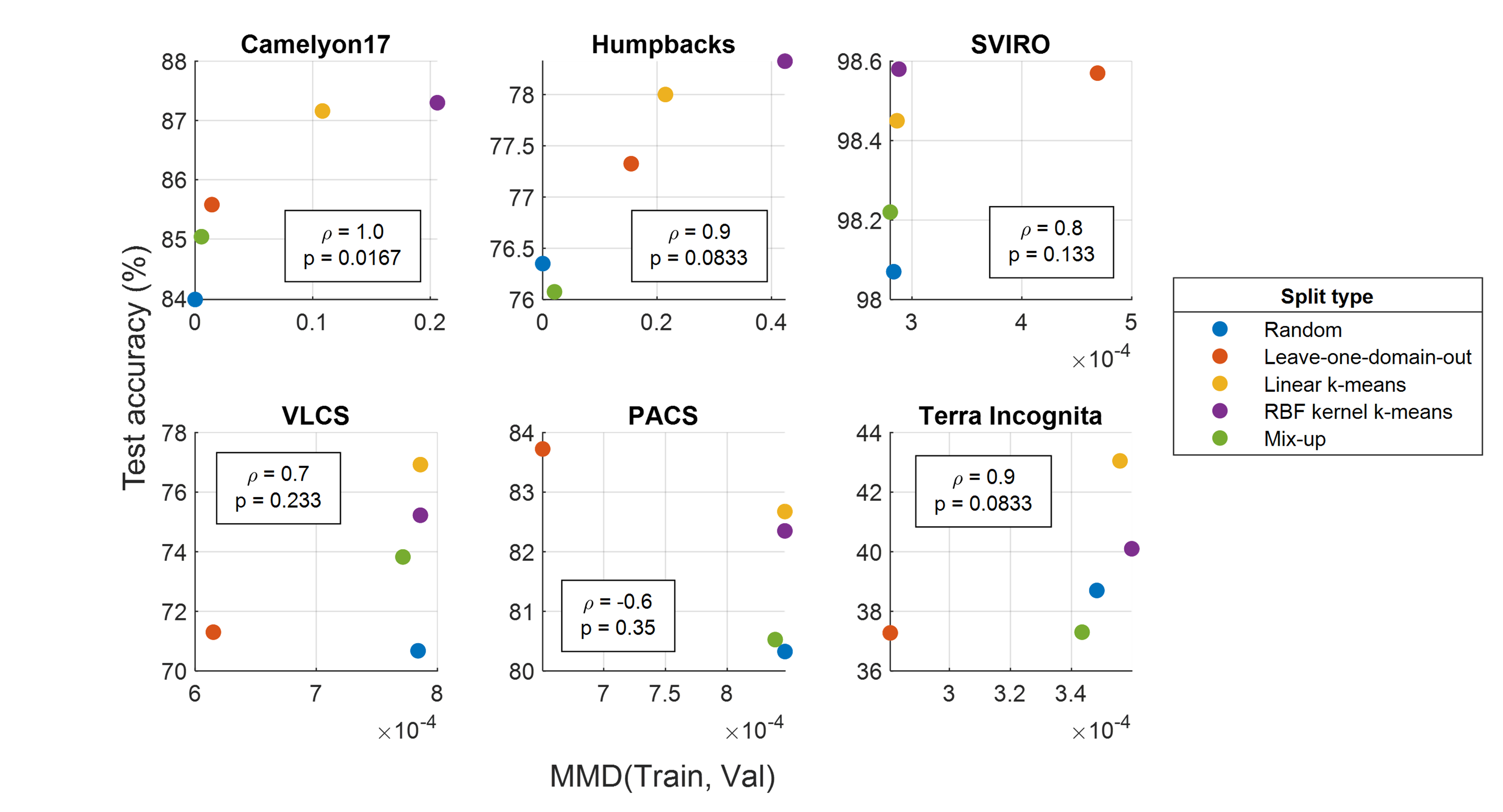
Figure 1: The MMD between the training and validation sets versus test domain accuracy, by dataset.

The leave-one-domain-out method often produced large outlier values for the MMD, which can be seen in Figure 1 for all datasets other than Camelyon17 and Humpbacks. The reason for these outliers is unclear. Nonetheless, the correlation for all datasets, with the exception of PACS, is positive.

Even with only 5 datapoints, Camelyon17 gives by far the clearest indication of a logarithmic-style relationship between the MMD and test accuracy, possibly because the dataset is large enough that a low-noise estimate of the MMD is possible. The results for this dataset are given in tabular form in Appendix D, along with an additional ablation comparing the different clustering constraints (1) and (2).

The results for all datasets plotted on a single set of axes are shown in Figure 2. As the ranges of both the accuracy and MMD values vary across datasets, these must be normalised in order to combine them. The median-IQR method (where each dataset is scaled to have zero median and unit interquartile range, on both axes) is used as this is the most robust to the large outliers mentioned. The MMDs are plotted on a symmetrical log scale [29] to make the correlation more visually evident. The means for each split type are also indicated.

Spearman’s $\rho$ for the combined datasets is 0.63, indicating a strong positive correlation between the MMD and test accuracy, whilst a $p$-value in the order of $10^{-4}$ indicates with strong significance that a rank correlation exists. Furthermore, Pearson’s $r$ coefficient for the log-scaled data in Figure 2 is calculated to be 0.61, with a $p$-value of $3.79\times 10^{-4}$. This $p$-value is for the test of the stronger hypothesis that the relationship between the two normalised variables is symmetrical-logarithmic, and again is strongly indicative that this is the case.

The evidence in this section supports the proposition that the validation split should be attempting to maximise the MMD between the training and validation sets, and that this is more effective than trying to create a domain shift of the same “type” as that of the test set, as a traditional metadata-based OOD validation split may do.

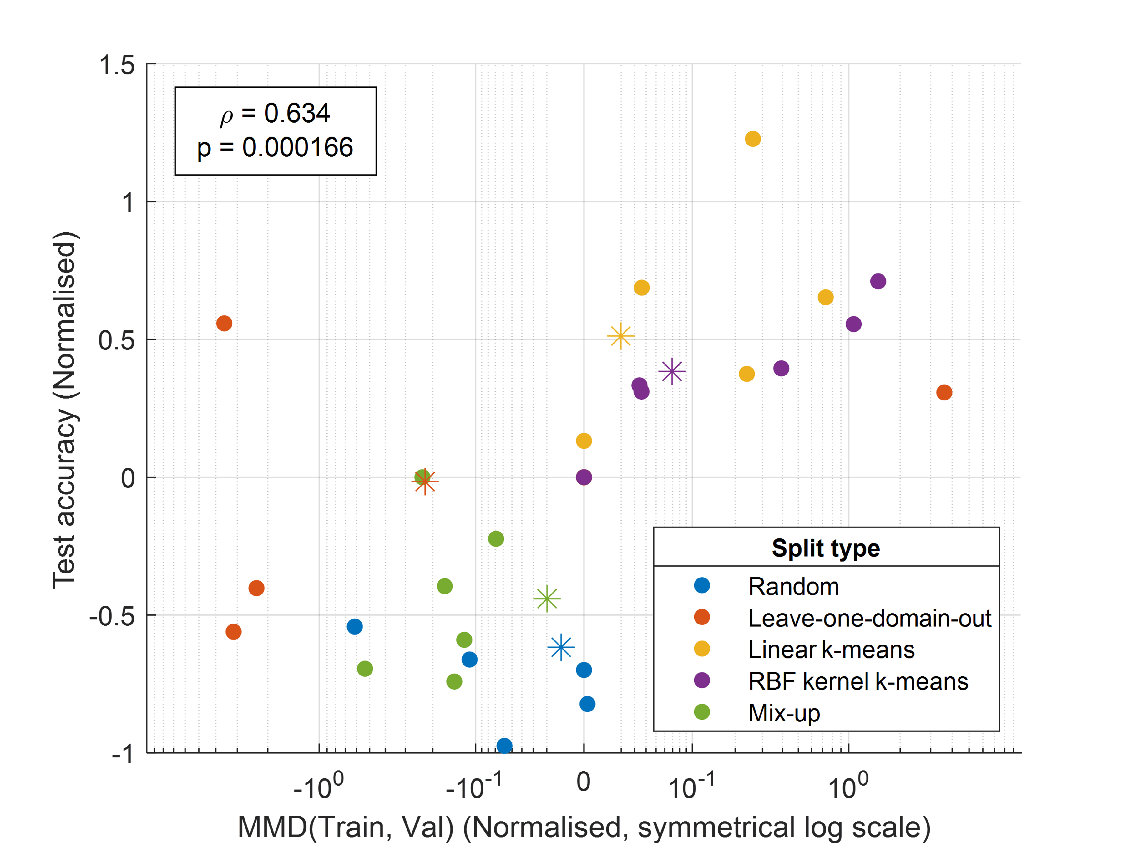
Figure 2: The MMD between the training and validation sets versus test domain accuracy, normalised by dataset, and plotted on a single set of axes. The mean for each split type is indicated with an asterisk ($*$). Note there are 6 overlaying datapoints at the origin, corresponding to the medians of each dataset.

2.4 Assessing the effect of the changing training distribution

The use of non-random data splitting introduces a confounding variable to the experiments: as both the training and validation distributions are dependent on the split, it is possible the test accuracy is being influenced by the model training, as well as the validation. To support the claim that cluster-based splitting results in more generalisable model selection, it is necessary to decouple the effects of these interventions, and show that it is indeed the improved model validation, and not the training, that is improving test accuracy.

As non-random data splitting inherently changes the training distribution, the effect of the model selection cannot be isolated from that of the training. However, the inverse – that is, varying the training distribution by changing the split type, but keeping the validation set constant – can be achieved, if the oracle selection criterion is used.

If the test accuracy remains constant across split types, this would be sufficient to verify the hypothesis that the performance improvements are due to the model selection, without having to make any additional assumptions. If the accuracy is lower than the random split, the hypothesis can still be confirmed (which then implies the model selection is additionally compensating for this reduction), as long as the effects of training and validation robustness on test accuracy are assumed to be additive (i.e., any interaction effects are minor). If anything, the non-random splits would be expected to underperform, since coverage of the overall data distribution by the training set is being reduced – and this would be expected to be detrimental to generalisation power. The results are given in Table 2.

Table 2: Test accuracy using the oracle criterion, for training sets induced by the different split types.

	DG experiments			UDA experiments
Split type	Camelyon17	Humpbacks	SVIRO	VLCS	PACS	TerraInc	Average
Random	88.3 ± 0.6	85.4 ± 1.5	99.1 ± 0.1	77.6 ± 0.5	84.4 ± 0.4	45.8 ± 1.0	80.1 ± 0.3
Leave-one domain out	85.4 ± 0.4	82.1 ± 1.3	99.0 ± 0.1	73.8 ± 0.3	82.2 ± 0.5	38.9 ± 1.2	76.9 ± 0.3
Linear k-means	88.0 ± 0.3	85.4 ± 0.8	99.1 ± 0.1	77.0 ± 0.3	85.7 ± 0.3	47.1 ± 0.9	80.4 ± 0.2
RBF kernel k-means	88.6 ± 0.6	85.0 ± 0.7	99.2 ± 0.1	77.9 ± 0.5	85.7 ± 0.3	44.5 ± 0.6	80.2 ± 0.2
Mix-up	88.3 ± 0.6	85.6 ± 1.6	99.2 ± 0.1	77.3 ± 0.5	84.4 ± 0.5	44.6 ± 0.9	79.9 ± 0.3

These results show that performing a cluster-based split has no significant effect on the generalisation power of a model trained on the training set produced by that split (that is, when the hyperparameters are being chosen via the oracle criterion). Therefore, it can be concluded that the change in performance of this method compared to the random split comes entirely from the model selection. On the other hand, test accuracy for the leave-one-domain-out split does significantly reduce. This finding may help to explain why metadata-based splits have been found to underperform random splits in some works [1]: the increased robustness of OOD validation is not enough to counterbalance the reduced robustness of training on fewer domains.

2.5 Limitations

Dataset and training algorithm choices for these experiments were biased towards combinations with larger performance gaps between the random split and oracle criteria. This was necessary to properly validate the method: it would be impossible to see any significant signs of improvement if the random split and oracle criterion were within margin of error. Although this does inevitably limit the scope of the experiments, it by no means invalidates the results: cluster-based splits do outperform random and metadata-based splits, where such an improvement is possible.

As stated in Section 1, a major advantage of clustering-based validation is that it is not dependent on domain metadata. However, even with the domain constraint removed or with metadata-independent training algorithms (e.g., ERM), the specific experimental setup in this paper precludes the ability to test this method in truly metadata-free settings. Due to the fundamental design of the DomainBed framework, domain metadata can still be leveraged (both implicitly and explicitly) through several avenues. For example, models are still trained on domain-balanced minibatches of data, and validation accuracy is averaged over the validation domains. The datasets themselves may also be unrealistically domain-balanced to begin with. However, the authors believe that these influences are mild enough that the overall trends observed in these experiments can reasonably be expected to hold in metadata-free settings as well.

The experiments would ideally be repeated across a range of model architectures to reflect the differences in generalisation power of larger/newer models. However, it was necessary to restrict the experiments in this paper to a single, smaller model (ResNet-18) due to the high computational costs involved in developing and comparing model selection criteria.

3 Conclusion

This paper presented a method for model selection under domain shift, where the training-validation split is performed using a constrained kernel k-means clustering algorithm. In addition to outperforming traditional methods, this approach is grounded by an observed strong correlation between the MMD between the training and validation sets, and test domain accuracy.

The algorithm is not parameter-free; future work could include a data-driven method for selecting these parameters, for example with an additional layer of meta-tuning. The algorithm can also trivially be extended to k-fold cross-validation by increasing the number of clusters.

Appendix A Additional training and hyperparameter details

Table 3: General parameter values and training details for the experiments.

Experimental parameter	Value
Hyperparameter random search size	10
Number of trials	3
Holdout fraction	0.2
UDA holdout fraction	0.5
Number of training steps	3000
Gaussian kernel bandwidth	1
Finetuning iterations before split	3000
Nyström subset size (if applicable)	2000
Architecture	ResNet-18
Class balanced	True

Table 4: Classification pipeline of the Humpbacks dataset. This follows the pipeline in [24].

Step number	Step detail
Acoustic front-end
1	Resample to 10 kHz
2	Mel-scale filter bank with 64 filters
3	Short-time Fourier transform with 100 ms FFT window, 50% overlap
4	Per-channel energy normalisation
5	Split into 3.92 s (128 pixel) analysis frames with 50% overlap
CNN
1	Conv2D (nodes=16, kernel=3x3, stride=2, activation=ReLU)
2	Conv2D (nodes=16, kernel=3x3, stride=2, activation=ReLU)
3	Conv2D (nodes=16, kernel=3x3, stride=2, activation=ReLU)
4	Conv2D (nodes=16, kernel=3x3, stride=2, activation=ReLU)
5	Global average-pooling 2D
6	Fully-connected layer

Appendix B Worst case accuracy validation

Table 5: Model selection using validation accuracy of the worst performing domain. Note that this does not apply to the leave-one-domain-out and oracle criteria, so these values are unchanged from Table 1.

	DG experiments			UDA experiments
Split type	Camelyon17	Humpbacks	SVIRO	VLCS	PACS	TerraInc	Raw average	Normalised average
Random	83.2 ± 1.6	76.7 ± 3.1	98.2 ± 0.2	69.7 ± 3.0	81.8 ± 0.9	40.2 ± 1.9	75.0 ± 0.8	0.0 ± 13.5
Leave-one domain out	85.6 ± 1.0	77.3 ± 1.7	98.6 ± 0.0	71.3 ± 3.5	83.7 ± 0.6	37.3 ± 2.5	75.6 ± 0.8	23.3 ± 12.1
Linear k-means	87.1 ± 0.2	77.8 ± 1.6	98.6 ± 0.1	73.7 ± 2.0	83.8 ± 0.6	42.3 ± 1.9	77.2 ± 0.5	49.8 ± 8.8
RBF kernel k-means	87.5 ± 0.7	78.2 ± 0.6	98.5 ± 0.2	76.8 ± 0.6	83.9 ± 1.0	38.8 ± 2.5	77.3 ± 0.5	46.8 ± 10.9
Mix-up	83.9 ± 0.8	76.9 ± 1.5	98.4 ± 0.2	72.9 ± 1.5	81.0 ± 0.5	38.3 ± 2.7	75.2 ± 0.6	2.3 ± 10.7
Oracle	88.3 ± 0.6	85.4 ± 1.5	99.1 ± 0.1	77.6 ± 0.5	84.4 ± 0.4	45.8 ± 1.0	80.1 ± 0.3	100.0 ± 5.7

Appendix C Ablation study

An ablation study conducted on the VLCS dataset is shown in Table 6. This shows the effects of finetuning the feature extractor before clustering, the Nyström approximation, and the different constraint sets (1) and (2).

Table 6: Ablation study on VLCS.

Kernel/ Split type	Finetuning $\theta_{F}$	Constraint groups	Full/ Nyström kernel	Accuracy (%)
Linear	True	$g\in\mathcal{Y\times D}$	Nyström	76.4 ± 0.4
RBF	True	$g\in\mathcal{Y\times D}$	Nyström	76.2 ± 0.6
Linear	True	$g\in\mathcal{Y}$	Full	72.4 ± 1.9
RBF	True	$g\in\mathcal{Y}$	Full	75.1 ± 0.9
Linear	True	$g\in\mathcal{Y\times D}$	Full	76.9 ± 0.1
RBF	True	$g\in\mathcal{Y\times D}$	Full	75.2 ± 0.8
Linear	False	$g\in\mathcal{Y\times D}$	Full	75.6 ± 0.8
RBF	False	$g\in\mathcal{Y\times D}$	Full	76.4 ± 0.5
Mix-up	True	N/A	N/A	73.8 ± 1.7
Leave-one-domain-out	True	N/A	N/A	71.3 ± 3.5
Random	True	N/A	N/A	70.7 ± 2.9
Oracle	True	N/A	N/A	77.6 ± 0.5

For this dataset, use of the Nyström approximation, as well as additional finetuning of $\theta_{F}$, are not observed to have significant effects on test accuracy. For the linear kernel, clustering with constraints (1) performs significantly lower than using constraints (2), however, for the RBF kernel, this difference is not observed.

Appendix D MMD analysis on Camelyon17

This table shows the MMD versus model accuracy on the Camelyon17 dataset (as in Figure 1), along with an additional ablation comparing the different clustering constraints (1) and (2). It can be seen that the additional constraint on the clustering (i.e., taking $g\in\mathcal{Y\times D}$) reduces the optimised objective function value (as would be expected), and this also corresponds to a reduction in test domain model accuracy.

Table 7: The MMD between the training and validation sets versus test domain accuracy by split type for Camelyon17.

Split type	Accuracy (%)	MMD ×1000
Random	84.0 ± 1.0	0.01 ± 0.0003
Mix-up	85.1 ± 0.4	5.4 ± 0.2
Leave-one-domain-out	85.6 ± 1.0	14.3 ± 0.8
Linear k-means ($g\in\mathcal{Y\times D}$)	86.5 ± 1.3	97.0 ± 6.2
RBF kernel k-means ($g\in\mathcal{Y\times D}$)	85.6 ± 1.3	183.1 ± 2.0
Linear k-means ($g\in\mathcal{Y}$)	87.2 ± 0.2	108.3 ± 2.6
RBF kernel k-means ($g\in\mathcal{Y}$)	87.3 ± 0.7	206.0 ± 3.4

References

- [1] Ishaan Gulrajani and David Lopez-Paz “In Search of Lost Domain Generalization” In ICLR, 2021
- [2] Pang Wei Koh et al. “WILDS: A Benchmark of in-the-Wild Distribution Shifts” In ICML ML Research Press, 2021
- [3] Martin Arjovsky, Léon Bottou, Ishaan Gulrajani and David Lopez-Paz “Invariant Risk Minimization” In arXiv, 2019
- [4] Shiori Sagawa, Pang Wei Koh, Tatsunori B Hashimoto and Percy Liang “Distributionally Robust Neural Networks for Group Shifts: On the Importance of Regularization for Worst-Case Generalization” In ICLR, 2019 URL: https://arxiv.org/abs/1911.08731v2
- [5] Ziwei Liu, Ping Luo, Xiaogang Wang and Xiaoou Tang “Deep Learning Face Attributes in the Wild” In Proceedings of International Conference on Computer Vision (ICCV), 2015
- [6] Aengus Lynch, Gbètondji J-S Dovonon, Jean Kaddour and Ricardo Silva “Spawrious: A Benchmark for Fine Control of Spurious Correlation Biases” In arXiv, 2023 URL: https://arxiv.org/abs/2303.05470v3
- [7] Irena Gao et al. “Out-of-Distribution Robustness via Targeted Augmentations” In ICML, 2023
- [8] Yoav Wald, Amir Feder, Daniel Greenfeld and Uri Shalit “On Calibration and Out-of-Domain Generalization” In NeurIPS 34, 2021, pp. 2215–2227
- [9] Boyang Lyu et al. “A principled approach to model validation in domain generalization” In ICASSP, 2023
- [10] Haotian Ye et al. “Towards a Theoretical Framework of Out-of-Distribution Generalization” In NeurIPS, 2021
- [11] Wang Lu, Jindong Wang, Yidong Wang and Xing Xie “Towards Optimization and Model Selection for Domain Generalization: A Mixup-guided Solution” In Proceedings of The KDD’23 Workshop on Causal Discovery, Prediction and Decision 218, Proceedings of Machine Learning Research PMLR, 2023, pp. 75–97 URL: https://proceedings.mlr.press/v218/lu23a.html
- [12] Dan Hendrycks and Thomas Dietterich “Benchmarking Neural Network Robustness to Common Corruptions and Perturbations” In ICLR International Conference on Learning Representations, ICLR, 2019 URL: https://arxiv.org/abs/1903.12261v1
- [13] Robert Geirhos et al. “ImageNet-trained CNNs are biased towards texture; increasing shape bias improves accuracy and robustness” In ICLR International Conference on Learning Representations, ICLR, 2018 URL: https://arxiv.org/abs/1811.12231v3
- [14] Zhiheng Li et al. “A Whac-A-Mole Dilemma: Shortcuts Come in Multiples Where Mitigating One Amplifies Others” In CVPR, 2022 URL: https://arxiv.org/abs/2212.04825v2
- [15] Dan Hendrycks et al. “Natural Adversarial Examples” In Proceedings of the IEEE Computer Society Conference on Computer Vision and Pattern Recognition IEEE Computer Society, 2019, pp. 15257–15266 DOI: 10.1109/CVPR46437.2021.01501
- [16] Anders Søgaard, Sebastian Ebert, Jasmijn Bastings and Katja Filippova “We Need To Talk About Random Splits” In Proceedings of the 16th Conference of the European Chapter of the Association for Computational Linguistics: Main Volume Online: Association for Computational Linguistics, 2021, pp. 1823–1832 DOI: 10.18653/v1/2021.eacl-main.156
- [17] Hanna Wecker, Annemarie Friedrich and Heike Adel “ClusterDataSplit: Exploring challenging clustering-based data splits for model performance evaluation” In Proceedings of Evaluation and Comparison of NLP Systems, 2020
- [18] Radha Chitta, Rong Jin, Timothy C. Havens and Anil K. Jain “Scalable Kernel Clustering: Approximate Kernel k-means” In arXiv, 2014 URL: https://arxiv.org/abs/1402.3849v1
- [19] I. Heller and C.B. Tompkins “An Extension of a Theorem of Dantzig’s” In Linear Inequalities and Related Systems, 1956
- [20] Baochen Sun and Kate Saenko “Deep CORAL: Correlation Alignment for Deep Domain Adaptation” In ECCV 9915 LNCS Springer Verlag, 2016, pp. 443–450 URL: https://arxiv.org/abs/1607.01719v1
- [21] Yaroslav Ganin et al. “Domain-Adversarial Training of Neural Networks” In JMLR Springer London, 2015
- [22] Gurobi Optimization LLC “Gurobi Optimizer Reference Manual”, 2023 URL: https://www.gurobi.com
- [23] Péter Bándi et al. “From Detection of Individual Metastases to Classification of Lymph Node Status at the Patient Level: The CAMELYON17 Challenge” In IEEE transactions on medical imaging 38.2 IEEE Trans Med Imaging, 2019, pp. 550–560 DOI: 10.1109/TMI.2018.2867350
- [24] Andrea Napoli and Paul White “Unsupervised Domain Adaptation for the Cross-Dataset Detection of Humpback Whale Calls” In DCASE, 2023
- [25] Steve Dias Da Cruz et al. “SVIRO: Synthetic Vehicle Interior Rear Seat Occupancy Dataset and Benchmark” In IEEE Winter Conference on Applications of Computer Vision (WACV), 2020
- [26] Chen Fang, Ye Xu and Daniel N. Rockmore “Unbiased metric learning: On the utilization of multiple datasets and web images for softening bias” In Proceedings of the IEEE International Conference on Computer Vision Institute of ElectricalElectronics Engineers Inc., 2013, pp. 1657–1664 DOI: 10.1109/ICCV.2013.208
- [27] Da Li, Yongxin Yang, Yi Zhe Song and Timothy M. Hospedales “Deeper, Broader and Artier Domain Generalization” In Proceedings of the IEEE International Conference on Computer Vision Institute of ElectricalElectronics Engineers Inc., 2017, pp. 5543–5551 DOI: 10.1109/ICCV.2017.591
- [28] Sara Beery, Grant Van Horn and Pietro Perona “Recognition in Terra Incognita” In ECCV 11220 LNCS Springer Verlag, 2018, pp. 472–489 URL: https://arxiv.org/abs/1807.04975v2
- [29] J. W. Webber “A bi-symmetric log transformation for wide-range data” In Measurement Science and Technology 24.2, 2013, pp. 027001 DOI: 10.1088/0957-0233/24/2/027001