Gaitor: Learning a Unified Representation Across Gaits for Real-World Quadruped Locomotion

Abstract

The current state-of-the-art in quadruped locomotion is able to produce robust motion for terrain traversal but requires the segmentation of a desired robot trajectory into a discrete set of locomotion skills such as trot and crawl. In contrast, in this work we demonstrate the feasibility of learning a single, unified representation for quadruped locomotion enabling continuous blending between gait types and characteristics. We present Gaitor, which learns a disentangled representation of locomotion skills, thereby sharing information common to all gait types seen during training. The structure emerging in the learnt representation is interpretable in that it is found to encode phase correlations between the different gait types. These can be leveraged to produce continuous gait transitions. In addition, foot swing characteristics are disentangled and directly addressable. Together with a rudimentary terrain encoding and a learned planner operating in this structured latent representation, Gaitor is able to take motion commands including desired gait type and characteristics from a user while reacting to uneven terrain. We evaluate Gaitor in both simulated and real-world settings on the ANYmal C platform. To the best of our knowledge, this is the first work learning such a unified and interpretable latent representation for multiple gaits, resulting in on-demand continuous blending between different locomotion modes on a real quadruped robot.

I Introduction

Recent advances in optimal control [1, 2, 3, 4, 5] and reinforcement learning (RL) [6, 7, 8, 9, 10] have enabled robust quadruped locomotion over uneven terrain. This has made quadrupeds a promising choice for the execution of inspection, monitoring and search and rescue tasks. Current state-of-the-art methods such as [11, 7] are highly capable and produce a variety of complex motions. However, these methods tend to be either engineered top-down, incorporating expert knowledge of the locomotion process via appropriate inductive biases, or bottom-up in a data-driven way. Typical examples of top-down approaches include leveraging the gait phase via an architectural inductive bias (e.g. [12, 13]) or selecting between different specialised policies to deliver individual skills (e.g. [6]). Such top-down approaches treat gaits as independent skills and are unable to benefit from synergies in terms of efficient learning or added capability beyond the prescribed skill set. In contrast, bottom-up methods tend to be black-box models of a blend of locomotion skills such as a single distribution over gaits learnt using a large transformer model [11]. While successful in terms of delivering locomotion capability, such models are typically unamenable to interpretation and generally do not yield insights into the emergence of the phenomenological inductive biases often used by domain experts when designing top-down approaches.

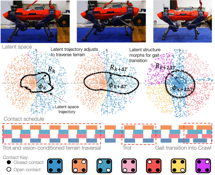
Figure 1: Gaitor is a data-driven approach to learning a single-disentangled representation for quadruped locomotion. This representation is expressive enough to capture the robot’s dynamics across multiple gaits (e.g. trot and crawl) and permits continuous gait transition via automatically discovered intermediaries. The latent space is conditioned using a rudimentary terrain encoding facilitating terrain traversal. A learnt planner in the latent space adjusts the gait characteristics in response to the terrain. The structure of the latent space alters as the operator demands a gait transition from trot to crawl.

A notable exception in the data-driven regime, albeit in the context of only a single gait type on flat ground, is VAE-Loco [14, 15]. VAE-Loco demonstrates that gait-phase relationships emerge when learning a disentangled latent representation based on relatively narrow demonstration data. In particular, the swing heights and lengths are encoded in two independent dimensions of VAE-Loco’s latent space. Modulating trajectories in this two-dimensional space results in independent control of the robot’s in-swing gait characteristics (e.g. swing heights and lengths) on-demand.

Inspired by VAE-Loco, and in contrast to related works modelling multiple gaits, in this paper we present Gaitor, a data-driven approach to learning and exploiting a single, unified representation of locomotion dynamics in a disentangled latent-space across multiple gaits.

While our work is located in the domain of quadruped locomotion, in contrast to other work in this area our overarching goal is not in the first instance to achieve state-of-the-art performance in this area, but to explore the challenges and opportunities afforded by learning a single, disentangled representational space to encode the synergies between traditionally separated locomotion skills. We demonstrate that the structured latent space learnt by Gaitor is expressive enough to capture not only the individual gaits, but also continuous transitions between them via intermediary contact patterns, which do not exist in the training data. Gaitor incorporates a rudimentary terrain encoding, which adapts the latent-space structure in response to the ground beneath the robot in a readily interpretable way. In particular, the swing characteristics are encoded differently in response to changes in terrain. Gaitor couples these representations with a learnt planner operating in the latent space, and results in robust terrain-aware trajectories capable of traversing significant obstacles. We demonstrate this capability on a real ANYmal C robot [16].

To the best of our knowledge, Gaitor is the first work that demonstrates how a data-driven approach can create a unified representation for multiple modes of locomotion via a disentangled latent-space. Gaitor demonstrates significant advances over VAE-Loco, which forms inspiration for this paper. The first improvement of Gaitor is to integrate a perception pipeline for uneven terrain traversal. Next, Gaitor uses a learnt planner to generate adaptive trajectories in the latent space using a polar coordinate framework to adjust the robot’s gait characteristics (footswing lengths and heights) to traverse terrain robustly. After training Gaitor, it is discovered that the latent space automatically restructures itself to represent distinct gaits such as trot, crawl and pace. In contrast, the latent space generated using VAE-Loco is static and oscillatory trajectories are injected into the space for blind operation on flat ground. As an operator requests a different gait, Gaitor’s latent space changes shape and novel unseen gait transitions are discovered. Note that the expert pace gait is unstable on the real robot hence only the crawl/pace gait is deployed using our method. Gait transitions arise since the learnt representation captures meaningful correlations across the gait types resulting in a two-dimensional planning manifold in which a variety of complex locomotion tasks are solved. In our experiments on the real ANYmal C robot, we show continuous gait transitions on-demand from trot to crawl to a crawl/pace hybrid and vision-aware climbing onto a $12.5\text{\,}\mathrm{cm}$ platform.

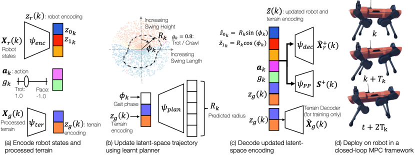
Figure 2: Gaitor learns a unified representation for locomotion dynamics across multiple gaits in a disentangled latent-space. There are three components to Gaitor. The first is a variational autoencoder (VAE) to encode the robot states and build the latent space and is comprised of an encoder $\psi_{enc}$ and decoder $\psi_{dec}$, see panels (a) and (c). The second is a terrain encoder $\psi_{ter}$ which estimates a rudimentary encoding of the ground ahead of the robot. Lastly, a learnt planner $\psi_{plan}$ creates trajectories in the latent space, see panel (b). The planner’s trajectory exploits the latent-space structure to vary the robot’s gait characteristics (footswing heights and lengths) in response to terrain. The operator can demand different gaits using the slider $g_{k}$ and this changes the structure of the latent space and results in an adjustment of the robot state trajectory and contact schedule. The updated latent-space trajectory is decoded to predict a set of future robot states ${\mathbf{X}}^{+}_{r}(k)$ and contact states ${\mathbf{S}}^{+}(k)$ using the performance predictor $\psi_{PP}$, see panel (c). The future trajectory is sent to a whole-body controller as depicted in panel (d).

II Related Work

Reinforcement learning (RL)  [8, 17, 10] is an increasingly popular choice for locomotion due to advances in simulation capabilities. A recent trend for RL is to solve locomotion problems by learning a set of discrete skills with a high-level planner arbitrating which skill is deployed at any one time. For example, [6] learns a set of $5$ distinct skills and a high-level planner to select the sub-skill to traverse the terrain ahead of the robot. These sub-skills include jumping across a gap or climbing over an obstacle. This method produces impressive behaviour, but no information is shared across tasks, meaning that each skill learns from scratch and correlations across skills are unused. Another impressive work Locomotion-Transformer [11] learns a generalist policy for multiple locomotion skills for traversing an obstacle course. This approach uses a transformer model to learn a multi-modal policy conditioned on terrain. In contrast, Gaitor learns a disentangled 2D representation for the dynamics of multiple locomotion gaits. The space infers the phase relationships between each leg and embeds these into the latent-space structure. Unseen intermediate gaits are automatically discovered by traversing this structured latent-space.

Work by [13] tackles gait switching by learning to predict the phases between each leg. The gait phase and the relative phases of each leg form this RL method’s action space. The predicted phases create a contact schedule for a model predictive controller (MPC), which computes the locomotion trajectory. In [13], the gait phase is an inductive bias designed to explicitly determine the swing and stance properties of the gait. The utilisation of the gait phase as an inductive bias for locomotion contact scheduling is common in the literature. For example, work by [12] conducted contemporaneously to Gaitor, utilises a latent space in which different gaits/skills are embedded. A gait generator operates from this space and selects a particular gait to solve part of the locomotion problem. This utilises a series of low-level skills prior to learn the latent representation using pre-determined contact schedules. In contrast, Gaitor infers the relationships between gait types and automatically discovers the intermediary gaits needed for smooth transitions from discrete examples.

Locomotion planning in learnt latent-representations is a growing field of interest. These methods are efficient at learning compact representations of robot dynamics. For example, [18] learns a latent action space and a low-level policy from expert demonstrations using imitation learning. Locomotion is achieved via an MPC formulation, which is solved via random shooting using a learnt dynamics model. Similarly, VAE-Loco [14] learns a structured latent-space in which the characteristics of the trot gait are disentangled. This structure is exploited leading to locomotion where the cadence, footstep height and length are varied continuously during the swing phase. VAE-Loco is constrained to a single gait and blind operation on flat ground only. This work forms the inspiration for Gaitor, which explores learning a single, unified latent representation for quadruped locomotion across multiple gaits to achieve perceptive locomotion in uneven terrains.

III Gaitor

This section outlines the components of Gaitor. A variational autoencoder (VAE) [19, 20] similar to VAE-Loco [14] is exposed to distinct gaits, trot, pace and crawl. This creates a shared representation across all the gaits and is conditioned on a learnt terrain encoding. Once the representation is created, a learnt planner is trained and operates in the latent space. This planner adjusts the robot’s gait characteristics in response to changing terrain.

III-A Overview

There are three components to Gaitor. These include a VAE [19, 20], a terrain encoder and planner in latent space. Fig. 2 (a) depicts the VAE’s encoder $\psi_{enc}$ and the terrain encoder $\psi_{ter}$. The VAE’s decoder $\psi_{dec}$ is shown in Fig. 2 (c). The VAE takes a history of robot states as input ${\mathbf{X}}_{r}(k)$ to infer the robot’s momentum via a robot encoding ${\mathbf{z}}_{r}(k)$ at the current time step $k$. The terrain encoder operates on processed information taken from a 2.5D representation of the ground around the robot to estimate ${\mathbf{z}}_{g}(k)$. The robot encoding and terrain encoding are concatenated with operator-controlled variables such as the desired gait label $g_{k}$ and the desired base velocity action ${\mathbf{a}}_{k}$. This concatenation is input into the decoder $\psi_{dec}$ and a performance predictor $\psi_{PP}$ [21] as depicted in Fig. 2 (c). The decoder reconstructs a small trajectory containing future predictions of the robot states $\hat{{\mathbf{X}}}^{+}_{r}(k)$. The performance predictor estimates which feet are in contact ${\mathbf{S}}^{+}(k)$ during the decoded trajectory. During deployment, the predicted trajectory is sent to a tracking controller which estimates the joint torques for the actuators.

The planner predicts a latent-space trajectory, which adapts the gait characteristics (e.g. footswing heights and lengths) in response to the terrain encoding. Similarly to VAE-Loco, inspection of Gaitor’s learnt latent-space in Sec. VI-C reveals that an elliptical trajectory in two dimensions of the representation is sufficient for independent control of the swing heights and lengths. Therefore, the latent-space planner is designed to predict an elliptical trajectory in polar coordinates, where the angle is equal to the gait phase $\phi_{k}$ and the radius is the planner’s output $R_{k}$ as seen in Fig. 2 (b). We explain how to process the data into the form required for the planner and its training regime in Sec. IV-B.

III-B Learning a Unified Representation

The VAE operates over the robot states only. The robot state at time step $k$ is ${{\mathbf{x}}_{k}=[{\mathbf{q}}_{k},\mathbf{ee}_{k},\mathbf{\tau}_{k},\mathbf{\lambda}_{k},\mathbf{\dot{c}}_{k},c_{\theta_{x}},c_{\theta_{y}},\Delta{\mathbf{c}}_{k}]}$ and represents the joint angles, end-effector positions in the base frame, joint torques, contact forces, base velocity, roll and pitch of the base and the base-pose evolution respectively. The VAE’s encoder $\psi_{enc}$ takes a history of these states as input. These samples are recorded at a frequency equal to $f_{enc}$. The input to the VAE is ${\mathbf{X}}_{k}$ and is constructed using $N$ past samples stacked together into a matrix. Similarly the output $\hat{{\mathbf{X}}}^{+}_{k}$ is a trajectory of states made from $M$ predictions into the future from time step $k$ sampled using a frequency $f_{dec}$. The robot’s base is floating in space and must be tracked so that the decoded trajectories can be represented in the world frame. The encoder tracks the evolution of the base pose $\Delta{\mathbf{c}}_{k}$ from a fixed coordinate. This coordinate is the earliest time point in the encoder input and all input poses are relative to this frame. All pose orientations are represented in tangent space. This is a common representation for the Lie-Algebra of 3D rotations since composing successive transformations using a Euclidean or a Quaternion representation is non-linear, but in tangent space, this composition is linear, see [22, 23] for examples. The output of the encoder parameterises a Gaussian distribution to create a latent-space estimate of the robot’s trajectory ${\mathbf{z}}_{r}(k)$.

The decoder predicts the future robot states $\hat{{\mathbf{X}}}^{+}_{r}(k)$ using the inferred latent variable and user-controlled inputs. This includes the base-pose evolution, which is expressed relative to the base pose at the previous time-step. The inputs to the decoder are ${\mathbf{z}}_{r}(k)$ the desired action ${\mathbf{a}}_{k}$, the desired gait label $g_{k}$, and terrain encoding ${\mathbf{z}}_{g}(k)$. Importantly, due to our formulation of learning a unified latent space across gaits, $g_{k}\in\mathbb{R}$ is a continuous value used to select a gait or intermediate gait type. Distinct gaits such as trot, crawl, and pace are selected when $g_{k}=\{1,0,-1\}$ respectively.

The performance predictor $\psi_{PP}$ estimates the contact states of the feet ${\mathbf{S}}(k)$ and takes the robot encoding as well as the desired action and gait as input, see Fig. 2. The contact states are predicted during operation and sent to the tracking controller to enforce the contact dynamics.

III-C Terrain Encoder

The terrain encoding is required so that the decoder and planner can react to terrain height variations. The robot’s perception module provides a 2.5D height map of the terrain. This is constructed from depth images from four depth cameras on the robot. This raw map is filtered and in-painted in a similar fashion to [24]. The height map is sampled at the locations of the next footholds and the heights ${\mathbf{h}}(k)$ are processed to create the terrain encoder’s input ${\mathbf{X}}_{g}(k)$. The processing pipeline takes the heights of the future footholds and finds the differences between left front, right hind and right front and left hind respectively. In this work, we define these relative differences as the control pitch $\theta_{c}$, see Fig. 3 (c). The control pitch varies discontinuously and only updates when the robot takes a step. To convert this discontinuous variable to a continuous one, we filter it using a second-order linear time-invariant (LTI) filter. This converts the step-like control pitch sequence into a continuous time varying signal ${\mathbf{X}}_{g}(k)$ of the type shown in Fig. 3 (d). This is achieved by setting the LTI’s rise time to occur when the foot in swing is at its highest point and using a damping factor of $0.5$. The input to the terrain encoder $\psi_{\mathrm{ter}}$ is a matrix of $N$ stacked values ${\mathbf{X}}_{g}(k)$ sampled at the control frequency $f_{c}$. The output of the terrain encoder ${\mathbf{z}}_{g}(k)$ forms part of the decoder’s input $\tilde{{\mathbf{z}}}(k)$ as shown in Fig. 2 (c). During training ${\mathbf{z}}_{g}(k)$ is input to a terrain decoder used to reconstruct a prediction of ${\mathbf{X}}_{g}(k)$. This element is discarded after training.

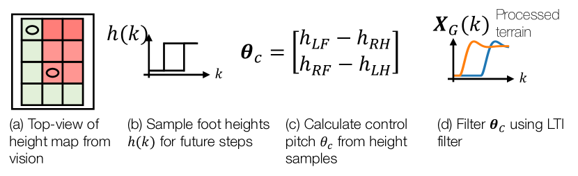
Figure 3: Terrain processing pipeline. The onboard perception module produces a 2.5D height map of the terrain around the robot. This map is sampled at the footfall positions to estimate the heights of the terrain at these locations, see panels (a) and (b). The control-pitch angle $\theta_{c}$ is defined as the difference in heights between the front and rear footfalls, see panel (c). These values are input to a second-order filter to create terrain encoder’s input ${\mathbf{x}}_{g}$ (panel (d)).

III-D Latent-Space Planner

The planner produces latent-space trajectories and is designed to adjust the robot’s swing length and height to help the robot traverse terrain. It is discovered in VAE-Loco [14] that the footswing heights and lengths are encoded into the two dimensions with lowest variance in latent space. These dimensions are denoted as $z_{0}$ and $z_{1}$ and a 2D elliptical trajectory in these dimensions controls the swing heights and lengths independently. In this paper, the same phenomenon is discovered in Sec. VI-C when the latent space is inspected as shown in Fig. 5. Therefore, we design the planner to exploit the disentangled space by only adjusting $z_{0}$ and $z_{1}$.

The planner is parameterised in polar coordinates and takes the gait phase $\phi(k)$ and terrain latent ${\mathbf{z}}_{g}(k)$ as input to predict the radius of the elliptical trajectory $R(k)$, see Fig. 2 (b). This trajectory updates the values of the two latent dimensions so that

$$\tilde{z}_{0}(k) =R(k)sin(\phi(k)),\quad$$ (1)

$$\tilde{z}_{1}(k) =R(k)sin(\phi(k)+\pi/2).$$ (2)

There are large variations in the values of $R(k)$ as is shown in Sec. VI-D. To ensure the planner reproduces these variations to a high fidelity, an architecture inspired by [25] is used as seen in Fig. 2 (b). The planner predicts a probability distribution $r_{c}$ for the radius over $C$ discrete values via a softmax. A weighted sum of the predicted probabilities multiplied by the bin values estimates the radius $R(k)$.

IV Training

In this section, we provide details on the loss functions used to train the individual components of Gaitor. The weights of the VAE and terrain AE are optimised in concert to help structure the latent space. The planner is trained last as it uses operates in the learnt space.

IV-A Training the VAE and Terrain AE

The VAE and performance predictor are optimised using the evidence lower bound (ELBO) and a binary cross entropy (BCE). The performance predictor estimates which feet are in contact ${\mathbf{S}}^{+}(k)$ given the robot-state input ${\mathbf{X}}_{r}(k)$. The BCE loss optimises the performance predictor’s parameters and gradients from this loss pass through the VAE’s encoder similarly to VAE-Loco [14]. It is found in VAE-Loco that backpropagating the BCE’s loss through the VAE’s encoder structures the latent space. Gaitor’s latent-space structure is inspected in Sec. VI-C. The ELBO loss used here takes the form of

$$\mathcal{L}_{\mathrm{ELBO}}=\mathrm{MSE}({\mathbf{X}}^{+}_{r}(k),\hat{{\mathbf{X}}}^{+}_{r}(k))+\beta D_{\mathrm{KL}}[q({\mathbf{z}}|{\mathbf{X}}_{r}(k))||p({\mathbf{z}})],$$ (3)

and is summed with the BCE loss creating

$$\mathcal{L}_{\mathrm{VAE}}=\mathcal{L}_{\mathrm{ELBO}}+\gamma\mathrm{BCE}({\mathbf{S}}^{+}(k),\hat{{\mathbf{S}}}^{+}(k)).$$ (4)

The VAE is optimised using GECO [26] to tune $\beta$ during training. Simultaneously, the terrain encoder’s weights are updated using the $\mathrm{MSE}$ loss between predicted $\hat{{\mathbf{X}}}_{g}(k)$ and the ground-truth data ${\mathbf{X}}_{g}(k)$ and gradients from the VAE decoder’s $\mathrm{MSE}$ loss. This creates the terrain autoencoder loss

$$\mathcal{L}_{\mathrm{TER}}=\mathrm{MSE}({\mathbf{X}}^{+}_{r}(k),\hat{{\mathbf{X}}}^{+}_{r}(k))+\mathrm{MSE}({\mathbf{X}}_{g}(k),\hat{{\mathbf{X}}}_{g}(k)).$$ (5)

The terrain decoder is only used for training purposes and is not required for deployment.

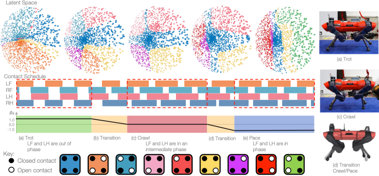
Figure 4: The latent-space structure encodes the contact schedule of the different gaits in distinct clusters (coloured segments). The same 2D slice of latent-space is plotted in all figures, and as the gait slider moves, the clustering of space changes smoothly. We include a key in the bottom row to map each coloured point in latent space to the stance phases of the robot. The phase between the front and rear legs shifts from out-of-phase for trot to in phase for pace via an intermediary phase, producing the crawl gait. The change in the phase is reflected in the structure of the latent-space: for trot the full-stance phase in blue is aligned horizontally. The full-stance phase rotates to the vertical for pace via the crawl gait structure. The trot, crawl and a dynamic crawl/pace hybrid gait are executed on the real robot in a single run lasting $50\text{\,}\mathrm{s}$. The expert pace gait is unstable on the real robot so we do not deploy any pace gaits on the real system.

IV-B Training the Planner

The planner in the latent space predicts the trajectory which is decoded to create the locomotion trajectory. In general, the planner can be trained using any framework such as an online or offline RL method, or a supervised learning approach. In this work, a behavioural cloning method is used to train the planner for simplicity. Expert trajectories are encoded into the VAE producing latent trajectories, ${\mathbf{z}}^{*}_{0},...,{\mathbf{z}}^{*}_{D}$, where $D$ is the number of time steps in the encoded episode. Only the dimensions $z_{0}$ and $z_{1}$ are retained to create the dataset for the planner and are converted to polar coordinates. Thus, $z^{*}_{0}(0),...,z^{*}_{0}(D)$ and $z^{*}_{1}(0),...,z^{*}_{1}(D)$ are converted to radii $R^{*}(0),...,R^{*}(D)$, and phases $\phi(0),...,\phi(D)$. The relationships between gait phase, radius and latent trajectories are

$$\phi(k) =\operatorname{atan2}(z^{*}_{0}(k),z^{*}_{1}(k))$$ (6)

$$R^{*}(k) =\sqrt{z^{*^{2}}_{0}(k)+z^{*^{2}}_{1}(k)}$$ (7)

The planner predicts the radius $R(k)$ given the gait phase $\phi(k)$ and the terrain encoding ${\mathbf{z}}_{g}(k)$ as inputs. The total loss is the sum between the MSE to reconstruct the target radius $R^{*}(k)$ and the cross-entropy loss between the prediction $r_{c}$ and the label $r^{*}$:

$$\mathcal{L}_{\mathrm{PLAN}}=\mathrm{MSE}(R(k),R^{*}(k))-\sum_{c=0}^{C-1}\log\Bigg{(}\frac{\exp(r_{c})}{\sum_{i=0}^{I-1}\exp(r_{c})}r^{*}\Bigg{)}.$$ (8)

V Deployment of Gaitor

The VAE, AE and its planner form a trajectory optimiser in a closed-loop controller. During deployment, the robot and terrain encodings are estimated using the VAE’s and AE’s encoders respectively. The operator chooses the base velocity action ${\mathbf{a}}_{k}$, the desired gait $g_{k}$ and the gait speed $\Delta\phi_{k}$. The gait speed $\Delta\phi_{k}$ controls the robot’s cadence (number of footfalls per minute) and updates the gait phase every time step as

$$\phi(k)=\phi(k-1)+\Delta\phi_{k}.$$ (9)

The latent-space planner uses the updated phase and the terrain encoding to predict the latent radius. This is used to overwrite dimensions $z_{0}$ and $z_{1}$ in the robot encoding ${\mathbf{z}}_{r}(k)$ as per Eq. (1). The updated encoding $\tilde{{\mathbf{z}}}(k)$ is formed by concatenating the updated robot encoding, the terrain encoding, action and gait label. It is then decoded using $\psi_{dec}$ and $\psi_{pp}$. The predicted joint angles, torques and future base-pose are extracted from $\hat{{\mathbf{X}}}^{+}(k)$ and are sent to a whole-body controller (WBC) [27]. During our deployment, we discovered a phase-lead is required for best base-orientation tracking. Therefore, we set the robot’s base pitch to the average of the control pitch $\theta_{c}$.

The entire approach operates on the CPU of the ANYmal C in a real-time control loop. There is a strict time budget of $2.5\text{\,}\mathrm{ms}$ for $400\text{\,}\mathrm{Hz}$ control. Therefore, we deploy Gaitor using a bespoke C++ implementation and vectorised code.

VI Experimental Results

Our evaluation of Gaitor is designed to address the following guiding questions: 1) What does the structure of the latent-space look like for multiple gaits and how do transitions occur? 2) How does the latent-space structure and the generated trajectory adjust to changes in terrain? 3) How do the capabilities of our method compare to the current state-of-the-art?

In the following sections we first describe the generation of the training dataset and detail hyper-parameter settings used for the experiments before addressing each of these questions.

VI-A Dataset Generation

Gaitor is effectively trained using a narrow set of skill demonstrations. The data used to train all components are generated using RLOC [17]. This employs a vision-based RL footstep planner and uses Dynamic Gaits [27] to solve for the task-space trajectories. The inputs to the controller are the desired base heading ${\mathbf{a}}_{k}$ and the raw depth map provided by the robot. We generate roughly $30\text{\,}\min$ of data of the robot traversing pallets of varying heights up to $12.5\text{\,}\mathrm{cm}$ in both trot and crawl. The pace gait is unable to traverse uneven terrain so data for pace are gathered on flat ground. Our implementation of Dynamic Gaits is unable to pace stably at speeds greater than $0.1\text{\,}\mathrm{m}\mathrm{/}\mathrm{s}$ in simulation and is unstable at all speeds on the real robot. Therefore, we do not deploy any pace gaits.

VI-B Architecture Hyper-parameters

The VAE’s encoder and decoder frequencies are set to $50\text{\,}\mathrm{Hz}$ and $400\text{\,}\mathrm{Hz}$. The input history contains $80$ timesteps, whilst the output predicts a small $20$ step trajectory. All networks are $256$ units wide and three layers deep with the robot latent-space and the terrain latent-space both of dimensionality $10$. The operator controlled base-heading action size is three units and the gait label is one unit. During terrain traversal, we utilise a desired swing-duration of $0.36\text{\,}\mathrm{s}$.

Figure 5: The latent space is disentangled and structured such that displacements in the horizontal $z_{0}$ axis increase the robot’s step height, whereas movements in the vertical axis $z_{1}$ correlate to the robot’s swing length.

VI-C The Latent-Space Structure Results in Gait Switching

Gaitor’s latent-space structure is investigated to understand how the space represents multiple gait types. Next, the space is explored revealing that continuous gait transitions are attainable using Gaitor. This analysis provides insights into how Gaitor represents shared information across gaits in the latent space and how transitions between gaits arise naturally as a result of the latent-space structure.

Inspecting the Latent-Space Structure: Inspired by VAE-Loco, we inspect the structure of the latent space. This reveals that Gaitor’s latent space is both structured and disentangled. In particular, the footswing lengths and heights are encoded into two orthogonal dimensions of the latent space, meaning that these gait characteristics can be controlled independently using trajectories in these dimensions. Furthermore, analysis reveals that these two latent-space dimensions ($z_{0}$ and $z_{1}$) have the lowest variance. Fig. 5 shows points in the 2D plane made up by $z_{0}$ and $z_{1}$. The points in this plane are colour coded by contact state, where orange corresponds to left front and right hind. Teal is the opposite contact state (right front and left hind), and blue represents all four feet in contact. The latent-space structure and its relationship to the contact states and schedules for multiple gaits are explored in the following sub-sections.

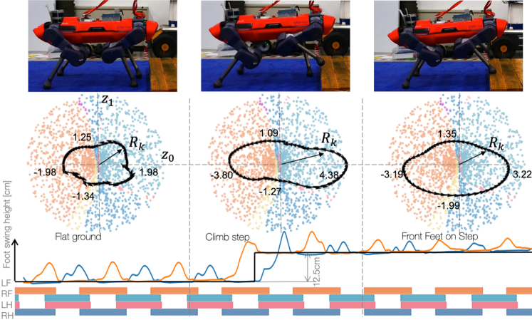
Figure 6: Gaitor deployed on the robot climbing a $12.5\text{\,}\mathrm{cm}$ platform. The planner and latent-space structure act in concert to alter the locomotion trajectories in response to the terrain. The first phase is flat ground where the planner produces a circular ellipse. When the robot steps onto the platform, the planner radius increases dramatically along the horizontal axis, but is reduced in the vertical axis compared to flat ground operation. This results in shorter footstep heights, but longer swing distances. Once both front feet are in contact with the elevated terrain, the latent-space trajectory returns to a broadly circular path.

Gait Switching: User-controlled and continuous gait switching from trot to crawl to a dynamic crawl/pace hybrid is observed when Gaitor is deployed on the real robot. The dynamic crawl/pace gait is characterised by a contact schedule where the hind foot makes contact as the front foot breaks contact simultaneously. To analyse the gait switching mechanism, latent dimensions $z_{0}$ and $z_{1}$ are plotted for a variety of gait types in Fig. 4. In Fig. 4, every point in latent space is colour-coded to denote which feet are in contact with the terrain, and Fig. 4 includes a key in the bottom row. As the gait label is toggled from $1.0$ (trot) to $-1.0$ (pace), the latent-space structure changes in concert with the contact schedule shown in the row below.

Gait Correlations: It is observed that Gaitor produces gait switching in a particular order: trot to crawl to pace and the reverse only. To investigate why gait transitions occur in this order, we inspect the latent-space structure for each gait and observe the phase relationships between legs during transition. During trot, the left front (LF) and left hind (LH) are out-of-phase with one another in the contact schedule (see row 2 of Fig. 4): the LF is in contact as the LH is in swing. However during pace, the LF and LH are in phase as these feet are swinging together. As the operator demands a gait transition from trot to pace or pace to trot, the crawl gait representation and contact schedule emerges at the midpoint of the transition. This is because the phase between the LF and LH is midway between in phase and out-of-phase for the crawl gait: only one foot swings at once during crawl. Gaitor is able to infer this relationship and uses it to represent the multiple different gaits in the representation efficiently. Furthermore, Gaitor finds intermediary latent-space structures to represent the contact schedules of the transitionary gaits e.g. trot/crawl or crawl/pace, see panel (b) and (d) in Fig. 4 and these produce smooth and continuous gait transitions. The ordering of the gaits in latent space using their in-phase relationships is similar to the analytical analysis found in [28]. The model used for quadruped kinematics in [28] consists of a pair of bipeds linked by a rigid body. Gaits are generated by varying the phases between the front and rear bipeds in a fashion similar to what here is inferred by Gaitor.

Feasibility Metrics: The quality of the gaits produced by Gaitor is measured using the joint-space error between input and output of the whole-body controller (WBC) measured over a $5\text{\,}\mathrm{s}$ window sampled at $400\text{\,}\mathrm{Hz}$. The WBC is an optimisation-based tracking controller and is able to adjust the VAE’s output to satisfy its dynamics constraints outlined in [29]. The root-mean-squared error (RMSE) is used as a measure of how optimal the VAE’s trajectories are with respect to the dynamics of the WBC. The RMSE for the trot, crawl and dynamic pace/crawl gaits are reported in Table I. In all cases the tracking error is low (less than $6\text{\,}\deg$), and is larger for the crawl and dynamic crawl gaits. The larger joint RMSE results from a small discrepancy between the robot’s actual and desired heights when operating in the crawl gaits.

	Dynamic Gaits (Trot)	Trot (Flat Ground)	Trot (Climb Phase)	Crawl	Dynamic Crawl/Pace
RMSE [rad]	0.021	0.012	0.013	0.058	0.098
Swing Height [cm]	8.5 $\pm$ 0.40	8.3 $\pm$ 0.58	9.68 $\pm$ 4.15	5.42 $\pm$ 0.65	6.22 $\pm$ 0.31
Swing Length [cm]	14.6 $\pm$ 3.99	10.4 $\pm$ 0.53	13.9 $\pm$ 1.65	-	-

TABLE I: The feasibility and gait characteristics for Gaitor and Dynamic Gaits, which is used to generate the training data. Gaitor’s gait characteristics and tracking root-mean-squared error (RMSE) values are recorded during four distinct modes of operation: trot on flat ground, trot whilst climbing the terrain, crawl gait, and the dynamic crawl/pace gait. The RMSE values are measured between the joint-space trajectories of the Gaitor or Dynamic Gaits and the whole-body controller’s (WBC) joint trajectories during a $5\text{\,}\mathrm{s}$ interval. The WBC uses a centroidal dynamics model to optimise the torque values. The lower the RMSE, the closer the VAE trajectories are to optimality under the assumptions of the WBC. All measurements are generated from experimental logs from real-robot experiments. The swing lengths are not measured for crawl and dynamic crawl as the robot is operated on the spot during these runs. Both trot data come from the terrain climb experiment, see Sec. VI-D.

VI-D Latent-Space Evolution During Terrain Traversal

Perceptive terrain-traversal is demonstrated using the trot gait to successfully climb a $12.5\text{\,}\mathrm{cm}$ step. During the climb phase, the nominal swing heights and lengths are observed to adjust in response to the terrain. In particular, the robot places its feet in a robust position further away from the edge of the step. To investigate how Gaitor produces this behaviour, the learnt planner’s trajectories in latent space are visualised and how the gait characteristics are encoded into the space is inspected. Finally, the feasibility of the Gaitor’s trajectories is compared to that of the dataset.

Figure 7: Level sets are plotted in latent space where isocontours decode to equal swing heights and lengths. The latent-space trajectories and isocontours are plotted during flat-ground operation (a) and as the robot approaches the step (b). The latent-space structure prioritises swing length during climb.

Latent-Space Trajectory In Response To Terrain: To investigate the planner’s response to the terrain, we plot the latent-space trajectory during three distinct phases of climbing the terrain in Fig 6. The first phase is nominal locomotion on flat ground (phase I), the second is a short transient (phase II), where the front feet step up onto the palette and the final is a new steady state (phase III), where the robot has its front feet on the terrain and its rear feet on the ground.

On flat ground the (phase I), the latent-space trajectory is broadly symmetrical and Gaitor produces locomotion with footswing heights and lengths of $8.3(0.58)\text{\,}\mathrm{cm}$ and $10.4(0.53)\text{\,}\mathrm{cm}$ respectively. During the climb, the planner more than doubles the nominal horizontal displacement of the latent-space trajectory from $1.98$ units to $4.38$ units, see the second row of Fig. 6. This results in a large increase in the swing length to $13.9(1.65)\text{\,}\mathrm{cm}$, but only a modest increase in swing height of $9.68(4.15)\text{\,}\mathrm{cm}$ in the robot’s base frame. As mentioned, this increases the robustness of the foothold selection as this footfall location is further from the edge of the step. This beneficial response of elongating only the footswing length is investigated in the next paragraph. In phase III, the latent trajectory returns to a more symmetrical shape similar to phase I. This is expected once the front feet have climbed the terrain, the locomotion is similar to flat ground operation.

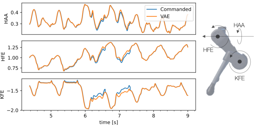
Figure 8: The joint-space trajectory in radians for the right front leg as it climbs terrain. The VAE’s joint space trajectory is tracked well by the WBC’s commanded values meaning that the VAE’s output is optimal with respect to the WBC’s dynamics formulation. A leg is plotted next to the tracking plots and annotated with the joint names.

Latent-Space Structure During Climb: During the climb (phase II), Gaitor increases the footswing length significantly more than the footstep height. This is investigated by inspecting how the encoding of the gait characteristics vary as the terrain changes. To visualise this, level sets in latent space are plotted in Fig. 7. Here, isocontours decode to locomotion trajectories with equal footswing height and length relative to the robot’s base frame. For example, decoding the inner most contour in Fig. 7 (a) results in locomotion with a footswing height and length of $8\text{\,}\mathrm{cm}$ (the swing length is measured relative to the base frame). For both flat-ground operation and the climb phase, the latent-space trajectories follow the isocontours. Crucially, as the edge of the pallet is encoded, the latent-space structure adapts such that a small displacement in the vertical axis of the latent space ($z_{1}$ dimension) decode to much longer footsteps. This is reflected in the planner’s trajectory which adjusts similarly to the latent-space structure to follow the deformation of the isocontours. If the flat-ground latent-trajectory is used during terrain traversal, the robot does not lift its feet high enough over the step and the feet collide with the step. However, Gaitor’s planner reacts to the oncoming terrain and produces a large footswing height with clearance of $4.6\text{\,}\mathrm{cm}$ above the edge of the pallet. In conclusion, the planner is necessary during terrain traversal in order to fully exploit the latent-space structure, which usefully deforms as the robot approaches terrain.

Approach	RL vs Representation Learning	Discovers Intermediate Skills	Explicit vs Implicit Representation
Caluwaerts et al. [11]	RL (Bottom-Up)	No	Implicit
Hoeller et al. [6]	RL (Top-Down)	No	Implicit
Yang et al.[13]	RL + MPC	No	Explicit Inductive Bias
Gaitor	Rep. Learn	Yes	Explicit Inferred

TABLE II: The characteristics and differentiating features of Gaitor are compared to a range of locomotion approaches. Bottom-up RL methods such as [11] tend to employ black-box models to learn a single distribution over multiple locomotion skills. Top-down RL refers to hierarchical approaches [6] to locomotion, which use a high-level planner to select a particular skill from a series of sub-policies optimised for one particular gait. RL and MPC methods in combination [13] tend to use RL to solve for trajectories constrained by difficult to model parts of the robot’s dynamics and use model-predictive control (MPC) to generate task-space trajectories. In contrast, Gaitor learns a unified representation across multiple gaits and in doing so is uniquely able to automatically discover new intermediate gaits and this ability is compared between approaches in the second column. The third column compares each method’s representation for locomotion. The first two RL methods have an internal implicit representation, whilst the Yang et al. [13] and Gaitor use the gait phase as explicit representation. The explicit representation of gait phase naturally leads to sharing of gait-specific correlations across skills and facilitates gait transitions as described in Sec. VI-C. However, Yang et al., use the gait phase as an inductive bias and a decision variable during training and execution. In contrast, Gaitor infers the gait phase across multiple gaits from expert examples of the trajectories.

Feasibility And Comparison To Expert: To quantify the feasibility of the Gaitor’s perceptive locomotion, we compute the joint-space error between the input and the output of the WBC. As before, root-mean-squared error (RMSE) is used to measure the optimality of the VAE’s trajectories with respect to the WBC’s centroidal dynamics [30]. The lower the RMSE value, the closer the VAE’s trajectory is to satisfying the WBC’s optimal solution. A $5\text{\,}\mathrm{s}$ window during flat ground operation and the climb phase (middle panel in Fig. 6) is compared with the dataset RMSE in Table I. The dataset uses the Dynamic Gaits [27] formulation, which is designed to operate with the WBC. The RMSE for the VAE during both flat-ground and climb phases is lower than that of Dynamic Gaits (see Table I) showing that Gaitor’s trajectories are feasible for the WBC to track with little to no adjustments. In contrast, the WBC makes minor adjustments to the trajectories from Dynamic Gaits, which accounts for the larger RSME values. In addition, the VAE’s joint trajectory, which is the input to the WBC and the WBC’s output (the commanded values) for the right-front leg are plotted in Fig. 8. The tracking error is insignificant (less than one degree) except during the initial touch down phase. This small increase in RMSE is attributed to vision error. The height of the step is slightly underestimated by the robot’s perception module, and does not affect the stability of the locomotion. After a subsequent footswing, the VAE adjusts and the tracking error remains extremely low.

VI-E Gaitor’s Capabilities in Relation to Other Methods

The characteristics of Gaitor and key differentiators are compared to current methods in Table II. As shown in Sec. VI-C, Gaitor is able to learn a unified representation across multiple gaits. In the same section, it is shown that this naturally yields continuous and smooth transitions between gaits in an interpretable way. Top-down hierarchical methods such as [6] use multiple independent policies and learn a planner to select the correct controller as required. This ignores correlations between the gait types and continous gait switching via intermediate gaits is impossible. Caluwaerts el al. [11] learn a multi-modal distribution policy over gait skills using a large transformer model. This does not produce an explicit representation, but an implicit one internal to the transformer. In contrast, Gaitor creates a dense and explicit latent-representation and once trained this representation facilitates the automatic discovery of useful intermediary gaits leading to smooth and continuous gait transitions in an interpretable way as seen in Sec. VI-C and Sec. VI-D. In particular, it is demonstrated in Sec. VI-C that Gaitor infers the correlations, namely the phase relationships, between the gait types and uses these to structure the latent representation. In essence, Gaitor has inferred an inductive bias from expert data that is typically used in the formulations of other methods. For example, [12, 13] uses the gait phase as an explicit control parameter to generate blind gait transitions. In contrast, Gaitor infers the gait phase relationship across gaits and builds this directly into its locomotion representation.

VII Limitations and Future Work

The focus of this paper is exploring the opportunities that learning a unified representation for locomotion across gaits provide and not pushing the state-of-the-art in one aspect of locomotion. As such, we have shown that Gaitor learns a representation capable of discovering continuous transitions between gaits and conditioned with a rudimentary terrain-encoding generates perceptive locomotion to traverse over significant obstacles. However, a number of limitations currently remain. The primary limitation of Gaitor is the requirement of high-quality expert demonstrations. We posit that this is a limitation currently of all learning-from-demonstration methodologies and is lessened by the availability of quality locomotion controllers designed for specific tasks/gaits.

In future, the latent-planner could be used to control the gait phase, desired heading and gait of the robot. These parameters are currently user-controlled and as we have shown in Sec. VI-C can be readily varied on-the-fly. A more sophisticated planner could be able to tackle more challenging locomotion tasks.

VIII Conclusions

In this paper, we explored the opportunities afforded by learning a single, disentangled representation for locomotion across gaits to encode correlations between separate skills. In doing so, we discovered that the learnt latent-space embeds not only each individual gait into the space, but also orders each gait representation such that continuous transitions via novel intermediary contact schedules are discovered from traversing the learnt latent-space. In addition, Gaitor incorporates a rudimentary terrain encoding which adapts the structure of the latent space and in conjunction with a learnt planner adjust the robot’s gait characteristics. During our evaluation of Gaitor, we investigate the gait transitions and terrain traversal. This reveals that the latent-space structure changes to represent different gaits during transition and adapts the gait characteristics in response to the terrain encoding. This change in gait characteristics is beneficial during the initial climb phase produces more robust footholds further away from the edge of the step. In conclusion, we show that learning a single unified latent representation for locomotion across gaits results in a methodology capable of continuous gait transitions and perceptive locomotion to traverse significant obstacles.

References

- [1] C. Mastalli, R. Budhiraja, W. Merkt, G. Saurel, B. Hammoud, M. Naveau, J. Carpentier, L. Righetti, S. Vijayakumar, and N. Mansard, “Crocoddyl: An efficient and versatile framework for multi-contact optimal control,” in IEEE Int. Conf. Rob. Autom. (ICRA), 2020.
- [2] C. Mastalli, W. Merkt, J. Marti-Saumell, H. Ferrolho, J. Sola, N. Mansard, and S. Vijayakumar, “A feasibility-driven approach to control-limited ddp,” Autonomous Robots, 2022.
- [3] R. Grandia, A. J. Taylor, A. D. Ames, and M. Hutter, “Multi-layered safety for legged robots via control barrier functions and model predictive control,” CoRR, 2020.
- [4] F. Jenelten, T. Miki, A. E. Vijayan, M. Bjelonic, and M. Hutter, “Perceptive locomotion in rough terrain – online foothold optimization,” IEEE Robot. Automat. Lett. (RA-L), vol. 5, no. 4, pp. 5370–5376, 2020.
- [5] O. Melon, R. Orsolino, D. Surovik, M. Geisert, I. Havoutis, and M. Fallon, “Receding-horizon perceptive trajectory optimization for dynamic legged locomotion with learned initialization,” in IEEE Int. Conf. Rob. Autom. (ICRA), 2021.
- [6] D. Hoeller, N. Rudin, D. Sako, and M. Hutter, “Anymal parkour: Learning agile navigation for quadrupedal robots,” 2023.
- [7] N. Rudin, D. Hoeller, M. Bjelonic, and M. Hutter, “Advanced skills by learning locomotion and local navigation end-to-end,” in 2022 IEEE/RSJ International Conference on Intelligent Robots and Systems (IROS), 2022, pp. 2497–2503.
- [8] S. Gangapurwala, A. Mitchell, and I. Havoutis, “Guided constrained policy optimization for dynamic quadrupedal robot locomotion,” IEEE Robot. Automat. Lett. (RA-L), vol. 5, no. 2, pp. 3642–3649, 2020.
- [9] J. Hwangbo, J. Lee, A. Dosovitskiy, D. Bellicoso, V. Tsounis, V. Koltun, and M. Hutter, “Learning agile and dynamic motor skills for legged robots,” Science Robotics, vol. 4, no. 26, 2019.
- [10] N. Rudin, D. Hoeller, P. Reist, and M. Hutter, “Learning to walk in minutes using massively parallel deep reinforcement learning,” 2022.
- [11] K. Caluwaerts, A. Iscen, J. C. Kew, W. Yu, T. Zhang, D. Freeman, K.-H. Lee, L. Lee, S. Saliceti, V. Zhuang, N. Batchelor, S. Bohez, F. Casarini, J. E. Chen, O. Cortes, E. Coumans, A. Dostmohamed, G. Dulac-Arnold, A. Escontrela, E. Frey, R. Hafner, D. Jain, B. Jyenis, Y. Kuang, E. Lee, L. Luu, O. Nachum, K. Oslund, J. Powell, D. Reyes, F. Romano, F. Sadeghi, R. Sloat, B. Tabanpour, D. Zheng, M. Neunert, R. Hadsell, N. Heess, F. Nori, J. Seto, C. Parada, V. Sindhwani, V. Vanhoucke, and J. Tan, “Barkour: Benchmarking animal-level agility with quadruped robots,” 2023.
- [12] J. Wu, Y. Xue, and C. Qi, “Learning multiple gaits within latent space for quadruped robots,” 2023.
- [13] Y. Yang, T. Zhang, E. Coumans, J. Tan, and B. Boots, “Fast and efficient locomotion via learned gait transitions,” in Conf. on Rob. Learn. (CoRL), 2021.
- [14] A. L. Mitchell, W. X. Merkt, M. Geisert, S. Gangapurwala, M. Engelcke, O. P. Jones, I. Havoutis, and I. Posner, “Vae-loco: Versatile quadruped locomotion by learning a disentangled gait representation,” IEEE Transactions on Robotics, pp. 1–16, 2023.
- [15] A. L. Mitchell, W. Merkt, M. Geisert, S. Gangapurwala, M. Engelcke, O. P. Jones, I. Havoutis, and I. Posner, “Next steps: Learning a disentangled gait representation for versatile quadruped locomotion,” in IEEE Int. Conf. Rob. Autom. (ICRA), 2022, pp. 10 564–10 570.
- [16] M. Hutter, C. Gehring, D. Jud, A. Lauber, C. D. Bellicoso, V. Tsounis, J. Hwangbo, K. Bodie, P. Fankhauser, M. Bloesch, R. Diethelm, S. Bachmann, A. Melzer, and M. Hoepflinger, “ANYmal - a highly mobile and dynamic quadrupedal robot,” in IEEE/RSJ Int. Conf. Intell. Rob. Sys. (IROS), 2016.
- [17] S. Gangapurwala, M. Geisert, R. Orsolino, M. Fallon, and I. Havoutis, “Rloc: Terrain-aware legged locomotion using reinforcement learning and optimal control,” IEEE Transactions on Robotics, vol. 38, no. 5, pp. 2908–2927, 2022.
- [18] T. Li, R. Calandra, D. Pathak, Y. Tian, F. Meier, and A. Rai, “Planning in learned latent action spaces for generalizable legged locomotion,” CoRR, vol. abs/2008.11867, 2020.
- [19] D. Kingma and M. Welling, “Auto-encoding variational bayes,” in Int. Conf. on Learn. Repr. (ICLR), 2014.
- [20] D. J. Rezende, S. Mohamed, and D. Wierstra, “Stochastic backpropagation and approximate inference in deep generative models,” in Int. Conf. on Mach. Learn. (ICML), 2014.
- [21] A. L. Mitchell, M. Engelcke, O. Parker Jones, D. Surovik, S. Gangapurwala, O. Melon, I. Havoutis, and I. Posner, “First steps: Latent-space control with semantic constraints for quadruped locomotion,” in IEEE/RSJ Int. Conf. Intell. Rob. Sys. (IROS), 2020, pp. 5343–5350.
- [22] J. Solà, J. Deray, and D. Atchuthan, “A micro lie theory for state estimation in robotics,” 2021.
- [23] C. Mastalli, W. Merkt, G. Xin, J. Shim, M. Mistry, I. Havoutis, and S. Vijayakumar, “Agile maneuvers in legged robots: a predictive control approach,” 2022. [Online]. Available: https://arxiv.org/abs/2203.07554
- [24] M. Mattamala, N. Chebrolu, and M. Fallon, “An efficient locally reactive controller for safe navigation in visual teach and repeat missions,” IEEE Robotics and Automation Letters, vol. 7, no. 2, pp. 2353–2360, apr 2022.
- [25] N. Ruiz, E. Chong, and J. M. Rehg, “Fine-grained head pose estimation without keypoints,” in 2018 IEEE/CVF Conference on Computer Vision and Pattern Recognition Workshops (CVPRW), 2018, pp. 2155–215 509.
- [26] D. J. Rezende and F. Viola, “Taming VAEs,” 2018.
- [27] C. D. Bellicoso, F. Jenelten, C. Gehring, and M. Hutter, “Dynamic locomotion through online nonlinear motion optimization for quadrupedal robots,” IEEE Robot. Automat. Lett. (RA-L), vol. 3, no. 3, pp. 2261–2268, 2018.
- [28] C. Tiseo, S. Vijayakumar, and M. Mistry, “Analytic model for quadruped locomotion task-space planning,” in 2019 41st Annual International Conference of the IEEE Engineering in Medicine and Biology Society (EMBC), 2019, pp. 5301–5304.
- [29] C. Dario Bellicoso, F. Jenelten, P. Fankhauser, C. Gehring, J. Hwangbo, and M. Hutter, “Dynamic locomotion and whole-body control for quadrupedal robots,” in IEEE/RSJ Int. Conf. Intell. Rob. Sys. (IROS), 2017, pp. 3359–3365.
- [30] D. Orin, A. Goswami, and S.-H. Lee, “Centroidal dynamics of a humanoid robot,” Autonomous Robots, vol. 35, 10 2013.