On the Convergence of Multi-objective Optimization under Generalized Smoothness

Abstract

Multi-objective optimization (MOO) is receiving more attention in various fields such as multi-task learning. Recent works provide some effective algorithms with theoretical analysis but they are limited by the standard $L$-smooth or bounded-gradient assumptions, which are typically unsatisfactory for neural networks, such as recurrent neural networks (RNNs) and transformers. In this paper, we study a more general and realistic class of $\ell$-smooth loss functions, where $\ell$ is a general non-decreasing function of gradient norm. We develop two novel single-loop algorithms for $\ell$-smooth MOO problems, Generalized Smooth Multi-objective Gradient descent (GSMGrad) and its stochastic variant, Stochastic Generalized Smooth Multi-objective Gradient descent (SGSMGrad), which approximate the conflict-avoidant (CA) direction that maximizes the minimum improvement among objectives. We provide a comprehensive convergence analysis of both algorithms and show that they converge to an $\epsilon$-accurate Pareto stationary point with a guaranteed $\epsilon$-level average CA distance (i.e., the gap between the updating direction and the CA direction) over all iterations, where totally $\mathcal{O}(\epsilon^{-2})$ and $\mathcal{O}(\epsilon^{-4})$ samples are needed for deterministic and stochastic settings, respectively. Our algorithms can also guarantee a tighter $\epsilon$-level CA distance in each iteration using more samples. Moreover, we propose a practical variant of GSMGrad named GSMGrad-FA using only constant-level time and space, while achieving the same performance guarantee as GSMGrad. Our experiments validate our theory and demonstrate the effectiveness of the proposed methods.

1 Introduction

There have been a variety of emerging applications of multi-objective optimization (MOO), such as online advertising [26], autonomous driving [18], and reinforcement learning [31]. Mathematically, the MOO problem takes the following formulation.

$$F^{*}=\min_{x\in\mathbb{R}^{m}}{F}(x):=(f_{1}(x),f_{2}(x),...,f_{K}(x)),$$ (1)

where $K$ is the total number of objectives and $f_{k}(x)$ is the $k$-objective function given model parameters $x$. Under the stochastic setting, $f_{k}(x)=\mathbb{E}_{s}[f_{k}(x;s)]$, where $s$ denotes data samples. This problem is challenging due to the gradient conflict that some objectives with larger gradients dominate the update direction at the sacrifice of significant performance degeneration on the less-fortune objectives with smaller gradients. A variety of MOO-based methods have been proposed to mitigate this conflict and find a more balanced solution among all objectives. In particular, the multiple gradient descent algorithm (MGDA) [12] aims to find a conflict-avoidant (CA) update direction that maximizes the minimal improvement among all objectives and converges to a Pareto stationary point at which there is no common descent direction for all objective functions. This idea then inspired numerous follow-up methods including but not limited to CAGrad [24], PCGrad [34], GradDrop [8], FAMO [23] and FairGrad [3] with a convergence guarantee in the deterministic setting with full-gradient computations. The theoretical understanding of the convergence and complexity of stochastic MOO is not well-developed until very recently. [25] proposed stochastic multi-gradient (SMG) as a stochastic version of MGDA, and established its convergence guarantee. [36] analyzed the non-convergence issues of MGDA, CAGrad and PCGrad in the stochastic setting, and further proposed a convergent approach named CR-MOGM. More recently, [13] and [6] proposed single-loop stochastic MOO methods named MoCo and MoDo, and proved their convergence to an $\epsilon$-accurate Pareto stationary point while guaranteeing an $\epsilon$-level average CA distance over all iterations. [32] proposed a double-loop algorithm named SDMGrad that enables to obtain an unbiased stochastic multi-gradient via a double-sampling strategy. They established the convergence of SDMGrad with a guaranteed $\epsilon$-level CA distance in every iteration, which we call as iteration-wise CA distance.

However, all existing works are limited by the standard $L$-smooth and bounded-gradient assumptions. Nevertheless, a recent study [35] indicates that such assumptions may not necessarily be true for the training of neural networks and an alternative $(L_{0},L_{1})$-smoothness condition was observed and studied, which assumes the Lipschitz constant to be linear in the gradient norm and the gradient norm to be potentially infinite. The analysis of existing MOO methods cannot be generalized to this $(L_{0},L_{1})$-smoothness directly due to the possible unbounded smoothness or gradient norm. In addition, all existing works [29, 35, 22, 21, 19, 11, 9] in generalized smoothness are limited to the single task problems, which are fundamentally different from the MOO problems. All of the above methods can not be directly generalized to the MOO tasks studied in this paper, since even though each single task is generalized smooth, the linear combination of these tasks is not necessarily generalized smooth. In this paper, we aim to fill this gap by proposing novel MOO algorithms, which not only converge under the generalized smoothness condition but also mitigate gradient conflict effectively with a guaranteed sufficiently small CA distance.

1.1 Our Contributions

We propose two single-loop MOO methods, Generalized Smooth Multi-objective Gradient descent (GSMGrad) and its stochastic variant SGSMGrad, and provide them with a comprehensive convergence analysis under the generalized smoothness condition in different settings. Our detailed contributions are listed below.

Weakest assumptions in MOO. In this paper, we investigate the $\ell$-smooth assumption, where $\ell$ is a general non-decreasing function of gradient norm, and includes both the standard $L$-smooth and $(L_{0},L_{1})$-smooth assumptions as special cases. This assumption finds many applications, such as transformers [35, 11], distributionally robust optimization [19] and higher-order polynomial functions [9]. In addition, we do not make any bounded-gradient assumption, which is required in previous analysis to ensure the bounded multi-gradient approximation. To the best of our knowledge, this is the first work to investigate generalized smoothness in MOO problems.

New single-loop algorithms. Both GSMGrad and SGSMGrad are easy to implement by updating the weights $w$ of objectives and model parameters $x$ simultaneously via a a single-loop structure. A warm-start initialization sub-procedure is also introduced at the beginning of both algorithms to ensure a sufficiently small iteration-wise CA distance under the single-loop structure. We also propose a computation- and memory-efficient variant of GSMGrad named GSMGrad-FA by updating the objective weights $w$ using only forward passes of $F(\cdot)$ rather than gradient $\nabla F$, which effectively reduces $O(K)$ time and space to $O(1)$ without hurting the performance guarantee.

Convergence analysis and optimal complexity. We provide a comprehensive analysis of our proposed algorithms under the generalized $\ell$-smooth condition in both deterministic and stochastic settings. To achieve an $\epsilon$-accurate Pareto stationary point and an $\epsilon$-level average CA distance, we show that GSMGrad and SGSMGrad require $\mathcal{O}(\epsilon^{-2})$ and $\mathcal{O}(\epsilon^{-4})$ samples in the deterministic and stochastic settings, respectively. Furthermore, to achieve a more aggressive $\epsilon$-level iteration-wise CA distance, GSMGrad and SGSMGrad require an increased number of samples, on the order of $\mathcal{O}(\epsilon^{-11})$ and $\mathcal{O}(\epsilon^{-17})$ respectively, in both deterministic and stochastic scenarios due to smaller step sizes and mini-batch data sampling. Moreover, we show that GSMGrad-FA achieves the same performance guarantee as GSMGrad.

Supportive experiments. Our experiments on the MTL benchmark Cityscapes [10] validate our theory and demonstrate the effectiveness of our proposed algorithms.

1.2 Related Works

Gradient-based multi-objective optimization. A variety of gradient manipulation techniques have emerged for simultaneous learning of multiple tasks. One prevalent category of methods adjusts the weights of various objectives according to factors such as uncertainty [20], gradient norm [7], and training complexity [17]. Methods based on MOO have garnered increased attention due to their systematic designs, enhanced training stability and model-agnostic nature. For instance, [30] framed Multi-Task Learning (MTL) as a MOO problem and introduced an optimization method akin to MGDA [12]. Afterward, many MGDA-based methods have been proposed to mitigate gradient conflict with promising empirical performance. Among them, PCGrad [34] avoids conflict by projecting the gradient of each task on the norm plane of other tasks. GradDrop [8] randomly drops out conflicted gradients. CAGrad [24] adds a constraint on the update direction to be close to the average gradient. NashMTL [27] and FairGrad [3] formulated MTL as a bargaining game and a resource allocation problem, respectively. Theoretically, [13] proposed a provably convergent stochastic MOO method named MoCo based on an auxiliary tracking variable for gradient approximation. [6] characterized the trade-off among optimization, generalization, and conflict avoidance in MOO. [32] proposed a stochastic MOO method named SDMGrad with a preference-oriented regularizer, and analyzed its convergence. However, all these works rely on the $L$-smoothness and bounded-gradient assumptions. This paper focuses on the MOO problems with generalized $\ell$-smooth objectives.

Generalized smoothness. The generalized $(L_{0},L_{1})$-smoothness was firstly proposed by [35], which was observed from extensive empirical experiments in training neural networks. A clipping algorithm was developed by[35] and the convergence rate was provided. Later, [19] analyzed the convergence of a normalized momentum method. The SPIDER algorithm was also applied to solve generalized smooth problems in [29, 9], where [9] studied a new notion of $\alpha$-symmetric generalized smoothness, which includes $(L_{0},L_{1})$-smoothness as a special case. Very recently, a new $\ell$-smoothness condition was studied in [21, 22], which is the weakest smoothness condition and includes all the smoothness conditions discussed above. However, all the existing works on generalized smoothness are limited to single-task optimizations and the understanding of MOO is insufficient. This paper provides the first study of MOO under the generalized $\ell$-smoothness condition.

2 Preliminaries

2.1 Generalized smoothness

The standard $L$-smoothness condition is widely investigated in existing optimization studies [15, 16], which assumes a function $f:\mathcal{X}\to\mathbb{R}$ to be $L$-smooth if there exists a bounded constant $L$ such that for any $x,y\in\mathcal{X}$, $\|\nabla f(x)-\nabla f(y)\|\leq L\|x-y\|.$ Nevertheless, recent studies show that in the training of neural networks such as transformers [35, 11], distributionally robust optimization [19] and high-order polynomials functions [9], the standard $L$-smoothness assumption does not hold. Instead, a generalized $(L_{0},L_{1})$-smoothness assumption was observed and studied in the training of transformers in [35], which assumes that for any $x\in\mathcal{X}$, $\|\nabla^{2}f(x)\|\leq L_{0}+L_{1}\|\nabla f(x)\|.$ This assumption implies the Lipschitz constant is potentially unbounded and reduces to the $L$-smoothness if $L_{1}=0$. Later, a more generalized assumption was proposed and studied in [21]:

Definition 1.

($\ell$-smoothness, Definition 1 in [21]). A real-valued differentiable function $f:\mathcal{X}\rightarrow\mathbb{R}$ is $\ell$-smooth if $\|\nabla^{2}f(x)\|\leq\ell(\|\nabla f(x)\|)$ almost everywhere in $\mathcal{X}$, where $\ell:[0,+\infty)\rightarrow(0,+\infty)$ is a continuous non-decreasing function.

The $(L_{0},L_{1})$-smoothness is a special case of $\ell$-smoothness, where $\ell(a)=L_{0}+L_{1}a$. There is another definition of generalized smooth, which is widely used and is equivalent to the $\ell$-smoothness:

Definition 2.

(($r,\ell$)-smoothness, Definition 2 in [21]). A real-valued differentiable function $f:\mathcal{X}\rightarrow\mathbb{R}$ is $(r,\ell)$-smooth if 1) for any $x\in\mathcal{X},B(x,r(\|\nabla f(x)\|))\in\mathcal{X}$, and 2) for any $x_{1},x_{2}\in B(x,r(\|\nabla f(x)\|)),\|\nabla f(x_{1})-\nabla f(x_{2})\|\leq\ell(\|\nabla f(x)\|)\|x_{1}-x_{2}\|$, where for continuous functions $r,\ell:[0,+\infty)\rightarrow(0,+\infty)$, $r$ is non-increasing, $\ell$ is non-decreasing and $B(x,R)$ is the Euclidean ball centered at $x$ with radius $R$.

In $B(x,r(\|\nabla f(x)\|))$, the function $f$ is also $L$-smooth where $L=\ell(\|\nabla f(x)\|)$. Proposition 3.2 in [21] shows that Definition 1 and Definition 2 are equivalent: An $(r,\ell)$-smooth function is $\ell$-smooth; and an $\ell$-smooth function satisfying Assumption 1 is $(r,m)$-smooth where $m(u):=\ell(u+a)$ and $r(u):=a/m(u)$ for any $a>0$.

2.2 Pareto concepts in multi-objective optimization (MOO)

As described before, MOO aims to find points at which there is no common descent direction for all objectives. Considering two points $x_{1},x_{2}\in\mathbb{R}^{m}$, we claim that $x_{1}$ dominates $x_{2}$ if $f_{i}(x_{1})\geq f_{i}(x_{2})$ for all $i\in[K]$ and $F(x_{1})\neq F(x_{2})$. We say a point is Pareto optimal if it is not dominated by any other point. In other words, we cannot improve one objective without compromising another when we reach a Pareto optimal point. In the general non-convex setting, MOO aims to find a Pareto stationary point defined as follows.

Definition 3.

We say $x\in\mathbb{R}^{m}$ is a Pareto stationary point if $\min_{w\in\mathcal{W}}\|\nabla F(x)w\|^{2}=0$. In practice, we call $x$ an $\epsilon$-accurate Pareto stationary point if $\min_{w\in\mathcal{W}}\|\nabla F(x)w\|^{2}\leq\epsilon^{2}$.

2.3 Multiple-gradient descent algorithm (MGDA) and its stochastic variants

Deterministic MGDA. One of the big challenges of MOO is the gradient conflict, i.e., the gradients of different objectives may vary heavily in scale such that the largest gradient dominates the update direction. As a result, the performance of those objectives with smaller gradients [34] may be significantly compromised. Towards this end, we tend to find a balanced update direction for all objectives. Thus, we consider the minimum improvement across all objectives and maximize it by solving the following problem

$$\max_{d\in\mathbb{R}^{m}}\min_{i\in[K]}\Big{\{}\frac{1}{\alpha}(f_{i}(x)-f_{i}(x-\alpha d))\Big{\}}\approx\max_{d\in\mathbb{R}^{m}}\min_{i\in[K]}\langle\nabla f_{i}(x),d\rangle,$$ (2)

where $\alpha$ is the step size, $d$ is the update direction, and the first-order Taylor approximation is applied at $x$. To efficiently solve the above problem in eq. 2, we substitute the following relation

$$\max_{d\in\mathbb{R}^{m}}\min_{i\in[K]}\langle\nabla f_{i}(x),d\rangle-\frac{1}{2}\|d\|^{2}=\max_{d\in\mathbb{R}^{m}}\min_{w\in\mathcal{W}}\Big{\langle}\sum_{k=1}^{K}\nabla f_{i}(x)w_{i},d\Big{\rangle}-\frac{1}{2}\|d\|^{2},$$ (3)

where $\mathcal{W}$ is the probability simplex over $[K]$, and the regularization term $-\frac{1}{2}\|d\|^{2}$ is to regulate the magnitude of our update direction. The solution to the problem in eq. 3 can be obtained by solving the following problem [32]

$$d^{*}=\nabla F(x)w^{*};\;\;s.t.\;w^{*}\in\arg\min_{w\in\mathcal{W}}\frac{1}{2}\|\nabla F(x)w\|^{2}.$$ (4)

The above approach has been widely used in e.g., deterministic MGDA and its variants such as CAGrad, and PCGrad [12, 34, 24].

Stochastic MGDA. SMG [25] is the first stochastic MGDA. It directly replaces the gradients with stochastic gradients and the update rule becomes

$$d_{s}^{*}=\nabla F(x;s)w_{s}^{*};\;\;s.t.\;w_{s}^{*}\in\arg\min_{w\in\mathcal{W}}\frac{1}{2}\|\nabla F(x;s)w\|^{2},$$ (5)

where $\nabla F(x;s)$ is the estimate of $\nabla F(x)$ based on the sample $s$. However, this leads to a biased gradient estimation of the update direction $d_{s}^{*}$, and thus it requires an increasing batch size. To solve this issue, another work MoCo [13] introduces a tracking variable $Y$ as a stochastic estimation of the true gradient. Afterward, a double-sampling strategy is proposed by [6, 32] to generate a near-unbiased update direction.

All the works mentioned above require bounded gradients such as [6, 13, 32] or $L$-smoothness such as [3, 24, 27, 33]. Their analyses do not apply to $\ell$-smoothness objectives studied in this paper, since the Lipschitz constant is potentially infinity.

2.4 Conflict-avoidant (CA) direction and CA distance

We call the update direction $d^{*}$ in eq. 4 the conflict-avoidant (CA) direction since it mitigates gradient conflict. Though it may not be feasible to calculate the exact CA direction, we aim to find an update direction to be close to the CA direction. Therefore, measuring the gap between the CA direction and the estimated update direction is important, which we define as the CA distance.

Definition 4.

$\|d-d^{*}\|$ is the CA distance between estimated update direction $d$ and CA direction $d^{*}$.

The larger the CA distance is, the further the estimated update direction will be away from the CA direction, and the more conflict there will be. In single-loop algorithms, MoCo and MoDo [13, 6], the average CA distance over iteration is of the order of $\epsilon$ while the double-loop algorithm SDMGrad [32] guarantees an $\epsilon$-order CA distance in every iteration. In our work, we analyze the CA distance in both cases and provide convergence results accordingly.

3 Single-loop Algorithms for MOO Under Generalized Smoothness

In this section, we present our main algorithms: Generalized Smooth Multi-objective Gradient descent (GSMGrad) and Stochastic Generalized Smooth Multi-objective Gradient descent (SGSMGrad), both are easy to implement with a simple single-loop structure. We also introduce an efficient variant of GSMGrad with constant-level computational and memory costs.

3.1 Generalized Smooth Multi-objective Gradient descent (GSMGrad)

We start to adopt MGDA in our method by computing an approximated weight $w_{t}$ and an update direction $d_{t}$ according to eq. 4 where $t$ is the iteration number. However, since the optimal weight $w^{*}$ of the convex function is not unique, we deal with this issue by adding an $\ell_{2}$ regularization term and the problem becomes

$$w_{\rho}^{*}=\arg\min_{w\in\mathcal{W}}\frac{1}{2}\|\nabla F(x)w\|^{2}+\frac{\rho}{2}\|w\|^{2}.$$ (6)

Besides the benefit of a unique solution, adding an $\ell_{2}$ regularization term also makes $w_{\rho}^{*}(x)$ Lipschitz continuous [13]. Note that $w^{*}(x)$ may not be Lipschitz continuous because $\nabla F(x)^{\top}\nabla F(x)$ may not be positive definite. Nevertheless, the analysis of CA distance is difficult because $w^{*}$ may not be Lipschitz continuous. Thus, we will characterize the gap between $w^{*}$ and $w_{\rho}^{*}$ plus the change of $w_{\rho}^{*}$ after adding this $\ell_{2}$ regularization term. As a result, the update rules become Lines 4-5 in Algorithm 1. We first update $w_{t}$ by a projected gradient descent process and compute the update direction $d_{t}=\nabla F(x_{t})w_{t}$ to update model parameters.

For our single-loop algorithm, CA distance is proportional to the term $\|w_{t}-w_{t,\rho}^{*}\|$, which decreases as the algorithm iterates with some error terms controlled by appropriately chosen small step sizes. If we initialize $w_{0}$ randomly, $\|w_{0}-w_{0,\rho}^{*}\|$ will be a constant order, and so will the first CA distance. Meanwhile, we can only get an $\epsilon$-order CA distance after a certain iteration number $t^{\prime}>1$ when $\|w_{t^{\prime}}-w_{t^{\prime},\rho}^{*}\|$ takes an $\epsilon$ order. Thus, we add an extra warm start process using Algorithm 2 to guarantee the new $w_{0}$ is close enough to $w_{0,\rho}^{*}$ and a small level CA distance in every iteration. However, this warm start process is not needed if we only require a small averaged CA distance.

Algorithm 1 Generalized Smooth Multi-objective Gradient descent (GSMGrad)

1:  Initialize: model parameters $x_{0}$, weights $w_{0}$ and a constant $\rho$

2:  $w_{0}$=Warm-start($w_{0}$, $x_{0}$, $\rho$) for small-level iteration-wise CA distance only

3:  for $t=0,1,...,T-1$ do

4:     $w_{t+1}=\Pi_{\mathcal{W}}\big{(}w_{t}-\beta[\nabla F(x_{t})^{\top}\nabla F(x_{t})w_{t}+\rho w_{t}]\big{)}$

5:     $x_{t+1}=x_{t}-\alpha\nabla F(x_{t})w_{t}$

6:  end for

Algorithm 2 Warm-start($w_{0}$, $x_{0}$, $\rho$)

1:  for $n=0,1,...,N-1$ do

2:     $w_{n+1}=\Pi_{\mathcal{W}}\big{(}w_{n}-\beta^{\prime}[\nabla F(x_{0})^{\top}\nabla F(x_{0})w_{n}+\rho w_{n}]\big{)}$

3:  end for

4:  Output $w_{N}$

3.2 Stochastic Generalized Smooth Multi-objective Gradient descent (SGSMGrad)

Under the stochastic setting, our algorithm keeps the same structure, having a warm start process and an update loop if we aim to control the CA distance in every iteration. In Algorithm 2, we do the same projected gradient descent without using stochastic gradients. This is because we only need to compute $\nabla F(x_{0})^{\top}\nabla F(x_{0})$ once and reuse it in the whole loop, which does not bring a computational burden. Then in the update loop, we update the weight and model parameters accordingly. We use a double-sampling strategy here to make the weight gradient estimator unbiased [32] such that $d_{t}$ is a near-unbiased multi-gradient $\mathbb{E}[\nabla G_{2}(x_{t})^{\top}\nabla G_{3}(x_{t})w_{t}+\rho w_{t}]=\nabla F(x_{t})^{\top}\nabla F(x_{t})w_{t}+\rho w_{t},$ where $\nabla G_{2}(x_{t})$ and $\nabla G_{3}(x_{t})$ are independent and unbiased estimates of $\nabla F(x_{t})$. Similarly, we do not involve a warm start process if we require the average CA distance to be small.

Algorithm 3 Stochastic Generalized Smooth Multi-objective Gradient descent (SGSMGrad)

1:  Initialize: model parameters $x_{0}$, weights $w_{0}$ and a constant $\rho$

2:  $w_{0}$=Warm-start($w_{0}$, $x_{0}$, $\rho$) for small-level iteration-wise CA distance only

3:  for $t=0,1,...,T-1$ do

4:     $x_{t+1}=x_{t}-\alpha\nabla G_{1}(x_{t})w_{t}$

5:     $w_{t+1}=\Pi_{\mathcal{W}}\big{(}w_{t}-\beta[\nabla G_{2}(x_{t})^{\top}\nabla G_{3}(x_{t})w_{t}+\rho w_{t}]\big{)}$

6:  end for

3.3 Fast approximation via Taylor expansion

Similarly to most MGDA-type algorithms, our methods require $\mathcal{O}(K)$ space and time to compute and store all task gradients at each iteration for updating the weight $w_{t}$. This becomes a drawback when the number of tasks or the model size is large. Motivated by [23], one solution is to use the Taylor Theorem to approximate the gradient for updating the weight $w_{t}$ as

$${F}(x_{t})-{F}(x_{t+1})=\nabla F(x_{t})^{\top}(x_{t}-x_{t+1})-R(x_{t})=\alpha\nabla F(x_{t})^{\top}\nabla F(x_{t})w_{t}-R(x_{t}),$$ (7)

where $R(x_{t})$ is the remainder term and it takes the order $R(x_{t})=o(\|x_{t}-x_{t+1}\|^{2})$, which can be made sufficiently small by adjusting the step size. Thus, we then propose GSMGrad-FA in Algorithm 4 (shown in Appendix B), where we update $x_{t}$ along the update direction $d_{t}=\nabla F(x_{t})w_{t}$ to get $x_{t+1}$ following by the update rule of $w_{t}$

$$w_{t+1}=\Pi_{\mathcal{W}}\Big{(}w_{t}-\beta\Big{[}\frac{F(x_{t})-F(x_{t+1})}{\alpha}+\rho w_{t}\Big{]}\Big{)}.$$ (8)

As a result, in the model parameters update process, we only require one backward process by calculating the gradient of $F(x_{t})w_{t}$ w.r.t. $x_{t}$ without storing it, and additional forward processes to compute $F(x_{t+1})$ in the weight update process. This approach saves computational and memory costs in the practical implementation significantly. More importantly, we also provide a theoretical guarantee for this efficient method (in eq. 8).

4 Convergence Analysis under Average CA distance

In this section, we provide the theoretical results for Algorithms 1 and 3 without warm starts to obtain an $\epsilon$-accurate Pareto stationary point, with the average CA distance over iterations in $\mathcal{O}(\epsilon)$.

4.1 Deterministic setting

Assumption 1.

Each objective function $f_{i}$ $\forall i\in[K]$ is twice differentiable and lower bounded by $f_{i}^{*}:=\inf_{x\in\mathbb{R}^{m}}f_{i}(x)>-\infty$.

Assumption 2.

Each objective function $f_{i}$ $\forall i\in[K]$ is $\ell$-smooth defined in Definition 1, where $\ell:[0,+\infty)\rightarrow(0,+\infty)$ is a continuous non-decreasing function such that $\varphi(a)=\frac{a^{2}}{2\ell(2a)}$ is monotonically increasing for any $a\geq 0$.

These assumptions are the most relaxed ones in existing MOO works since they directly assume objective smoothness or gradient/function value boundness [24, 13, 27, 32, 6, 33, 3]. It also includes the widely studied standard $L$-smoothness [28, 15, 16], $(L_{0},L_{1})$-smoothness [35] as special cases. Moreover, for any $0\leq\gamma\leq 2$ and $x\in\mathcal{X}$, our assumption even holds for function $f$ such that $\|\nabla^{2}f(x)\|\leq L_{0}+L_{1}\|\nabla f(x)\|^{\gamma}$, where $\gamma$ are limited to $[0,1]$ in [9].

We then provide our theoretical results. Let $c>0$ and $F>0$ be some constants such that $\Delta+c\leq F,$ where $\Delta=\max_{i\in[K]}\{f_{i}(x_{0})-f^{*}\}$. Define $M=\sup\{z\geq 0|\varphi(z)\leq F\}$. We then have the following convergence rate for Algorithm 1:

Theorem 1.

Let Assumptions 1 and 2 hold. Set $\beta\sim\mathcal{O}(\frac{1}{M^{2}}),\alpha\sim\mathcal{O}(\frac{1}{M^{2}}+\frac{1}{M\ell(M+1)}),T\geq\max\left(\Theta\left(\frac{1}{\alpha\epsilon^{2}}\right),\Theta\left(\frac{1}{\beta\epsilon^{2}}\right)\right),$ and $\rho\sim\mathcal{O}(\epsilon^{2})$. We then have that $\frac{1}{T}\sum_{t=0}^{T-1}\|\nabla F(x_{t})w_{t}\|^{2}\leq\epsilon^{2}.$

The full version with detailed constants and detailed proof can be found in Appendix C.1. Theorem 1 provides the first convergence rate to obtain an $\epsilon$-accurate Pareto stationary point for MOO problems with $\ell$-smooth objectives. Moreover, it achieves the optimal sample complexity in the order of $\mathcal{O}(\epsilon^{-2})$for GD with a single standard $L$-smooth objective[5]. The MOO problems with $\ell$-smooth objectives are challenging due to two reasons: 1) $\|\nabla F(x)\|$ is potentially unbounded in our $\ell$-smoothness setting, making all existing analysis in MOO [24, 13, 27, 32, 6, 33, 3] not applicable. 2) the update of $x$ includes all gradient information from each task, making the existing adaptive methods for single generalized smooth functions invalid.

To solve the challenges in Theorem 1, we find that a bounded function value implies a bounded gradient norm. Thus in our proof, we use induction to show that with parameters selected in Theorem 1, for any $w\in\mathcal{W}$ and $t\leq T$, we have that $F(x_{t})w$ is upper bounded by $F$. Consequently, for any $i\in[K]$, we have that $\|\nabla f_{i}(x)\|\leq M$, which solves the unbounded gradient norm problem in our generalized smoothness setting. Then we can show that $\|\nabla F(x_{t})w_{t}\|$ converges.

Corollary 1.

Under the same setting in Theorem 1, $\frac{1}{T}\sum_{t=0}^{T-1}\|\nabla F(x_{t})w_{t}-\nabla F(x_{t})w_{t}^{*}\|^{2}=\mathcal{O}(\epsilon^{2})$.

The proof is available in Appendix C.2. Corollary 1 shows that the average CA distance converges.

4.2 Stochastic setting

In the stochastic setting, we assume that we have access to an unbiased stochastic gradient ${\nabla}f_{i}(x;s)$ instead of the true gradient $\nabla f_{i}(x)$, where $s$ is the collected samples. To prove convergence, we have the following assumption.

Assumption 3.

There exists some $\sigma\geq 0$ such that $\mathbb{E}[\|{\nabla}f_{i}(x;s)-\nabla f_{i}(x)\|^{2}]\leq\sigma^{2}$ for any $i\in[K]$.

Assumption 3 indicates bounded gradient variances, which is widely studied [32, 21, 13].

Let $s_{t,i}=(s_{t,i,1},s_{t,i,2},...,s_{t,i,k})$ be the $i$-th collection of samples at time $t$ in the stochastic model and $F(x_{t};s_{t,i})=(f_{1}(x_{t};s_{t,i,1}),f_{2}(x_{t};s_{t,i,2}),...,f_{k}(x_{t};s_{t,i,k})).$ In this section, we choose $G_{i}(x_{t})=F(x_{t};s_{t,i})$ for any $i\in[3]$. Define $\varepsilon_{t,i}=(\varepsilon_{t,i,1},\varepsilon_{t,i,2},...,\varepsilon_{t,i,k})=\nabla F(x_{t})-\nabla G_{i}(x_{t})$.

Let $F,c>0$ and $0<\delta\leq\frac{1}{2}$ be some constants such that $F\geq\frac{4(\Delta+c)}{\delta}$ and $M=\sup\{z\geq 0|\varphi(z)\leq F\}$. Define the following random variables $\tau_{1}=\min\{t|\exists i\in[K],f_{i}(x_{t+1})-f_{i}^{*}>F\}\wedge T,\tau_{2}=\min\{t|\exists i\in[K],j\in[3],\|\varepsilon_{t,j,i}\|>\frac{L_{0}}{\sqrt{\alpha\rho}}\}\wedge T,\tau_{3}=\min\{t|\exists i,j\in[K],\|\varepsilon_{t,2,i}\|\|\varepsilon_{t,3,j}\|>\frac{L_{1}}{\sqrt{\alpha\rho}}\}\wedge T$ and $\tau=\min\{\tau_{1},\tau_{2},\tau_{3}\}$, where $L_{0},L_{1}>0$ are some constants and $a\wedge b$ denotes $\min(a,b)$. We have the following theorem:

Theorem 2.

Let Assumptions 1, 2, and 3 hold. Set $\alpha\leq\min\{\mathcal{O}(\ell(M+1)),\mathcal{O}(\beta),\mathcal{O}(\rho),\mathcal{O}\left(\frac{1}{\sqrt{T}}\right),\mathcal{O}(\epsilon^{2})\}$, $\beta\leq\min\{\mathcal{O}\left(\frac{1}{\alpha{T}}\right),\mathcal{O}(\epsilon^{2}),\mathcal{O}(\rho)\}$, $\rho\leq\min\{\mathcal{O}\left(\frac{1}{\alpha T}\right),\mathcal{O}(\frac{1}{\sqrt{\alpha T}}),\mathcal{O}\left(\frac{\epsilon}{\sqrt{\beta}}\right),\mathcal{O}(\epsilon^{2})\}$ and $T\geq\Theta\left(\frac{1}{\alpha\epsilon^{2}}+\frac{1}{\epsilon^{4}}\right)$. We then have that $\frac{1}{T}\sum_{t=0}^{T-1}\|\nabla F(x_{t})w_{t}\|^{2}\leq\epsilon^{2},$ with the probability at least $1-\delta$.

The full version and detailed proof can be found in Appendix C.3. When we set $\alpha,\beta,\rho\sim\mathcal{O}(\epsilon^{2})$ and $T\sim\mathcal{O}(\epsilon^{-4})$, we can find an $\epsilon$-stationary point with the optimal sample complexity in the order of $\mathcal{O}(\epsilon^{-4})$ for SGD with a single $L$-smooth objective[1]. Note that in the proof of Theorem 1, we show for each $t\leq T$ and $w\in W$, we have that $F(x_{t})w$ is bounded by applying a small constant step size $\alpha$ and $\beta$. However, this condition does not necessarily hold for our stochastic setting due to the unbounded gradient noise. To solve this problem, we introduce stopping time $\tau$. The advantages are as follows: 1) for any $t\leq\tau$, $w\in W$, we have that $F(x_{t})w$ is bounded; 2) for any $t<\tau$, the norm of gradient noise is bounded; 3) due to the optimal stopping theorem, for any $w\in W$ and $i\in[3]$, we have that $\mathbb{E}[\sum_{t=0}^{\tau}\varepsilon_{t,i}w]=0$. Based on these properties, we can further get the following lemma:

Lemma 1.

Using the parameters selected in Theorem 2, we have that

$$\mathbb{E}[F(x_{\tau})w]-F^{*}w\leq\frac{\delta F}{8}-\frac{\alpha}{2}\mathbb{E}\left[\sum_{t=0}^{\tau-1}\|\nabla F(x_{t})w_{t}\|^{2}\right].$$ (9)

The proof of Lemma 1 is available in C.4. Lemma 1 indicates that $\frac{\alpha}{2}\mathbb{E}\left[\sum_{t=0}^{\tau-1}\|\nabla F(x_{t})w_{t}\|^{2}\right]$ is bounded by some constant and if $\tau=T$ with high probability, we have that $\frac{1}{T}\mathbb{E}\left[\sum_{t=0}^{T-1}\|\nabla F(x_{t})w_{t}\|^{2}\Big{|}\tau=T\right]\sim\mathcal{O}\left(\frac{1}{\alpha T}\right)$. Note that $\{\tau<T\}=\{\tau_{2}<T\}\cup\{\tau_{3}<T\}\cup\{\tau_{1}<T,\tau_{2}=T,\tau_{3}=T\}.$ The first two events are related to the gradient noise, where the probabilities can be bounded by Assumption 3 and Chebyshev’s inequality. The last event indicates that for some $i\in[K]$, we have $f_{i}(x_{\tau})-f_{i}^{*}\leq\frac{F}{2}.$ Based on Lemma 1 and Markov inequality, we can show that $\mathbb{P}(\{\tau_{1}<T,\tau_{2}=T,\tau_{3}=T\})\leq\frac{\delta}{4}$ and we can further show that $\mathbb{P}(\tau=T)\geq 1-\frac{\delta}{2}$. We then have that $\frac{1}{T}\sum_{t=0}^{T-1}\|\nabla F(x_{t})w_{t}\|^{2}$ converges with high probability. Similar to Corollary 1, Theorem 2 also implies the average of CA distances converges with time with high probability.

5 Convergence Analysis under Iteration-wise CA distance

In Section 4 we show that the average CA distance is bounded under generalized smooth conditions. The average CA distance is also studied in MoCo [13] and MoDo [6] with the bounded gradient assumption and these works only focus on guarantees of the average CA distance over iterations. However, a $\epsilon$-level average CA distance only implies the smallest CA distance to be $\epsilon$-level. Since we want to keep the update direction close enough to the CA direction, it is better to have a tighter bound of CA distances. In this section, we show the CA distance is $\mathcal{O}(\epsilon)$ at every iteration with the help of a warm-start process and convergence results for Algorithms 1, 3, and 4.

5.1 Deterministic setting

Deterministic setting without fast approximation. We first provide results about bounded iteration-wise CA distance for Algorithm 1 with a warm start.

Theorem 3.

Let Assumptions 1 and 2 hold. Set $\beta^{\prime}\leq\frac{1}{M^{2}},\rho\sim\mathcal{O}(\epsilon^{2}),\beta\sim\mathcal{O}(\epsilon^{4}),\alpha\sim\mathcal{O}(\epsilon^{9})$, $N\sim O(\epsilon^{-2})$ as constants, and $T\sim\Theta(\epsilon^{-11})$. All the parameters satisfy the requirements in the formal version of Theorem 1 and we have $\|\nabla F(x_{t})w_{t}-\nabla F(x_{t})w_{t}^{*}\|\sim\mathcal{O}(\epsilon).$

The finite time error bound and the full proof can be found in Appendix D.1. Since our parameters satisfy the requirements in the formal version of Theorem 1, we can find an $\epsilon$-accurate Pareto stationary point with $\mathcal{O}(\epsilon^{11})$ samples. In the analysis of CA distance, we show that the CA distance can be bounded by the term $\|w_{t}-w_{t,\rho}^{*}\|$ plus the strongly-convex constant $\rho$. Meanwhile, there is a decay relation between $\|w_{t+1}-w_{t+1,\rho}^{*}\|$ and $\|w_{t}-w_{t,\rho}^{*}\|$ with some error terms controlled by step sizes. Nevertheless, the error terms will accumulate since we do telescoping on this decay relation, which will be the dominating term. Thus, step sizes have to be much smaller than the choices in Theorem 1 to guarantee iteration-wise small CA distance.

Deterministic setting with fast approximation. In this section, we show the convergence rate of Algorithm 4 and bounded iteration-wise CA distance.

Theorem 4.

Let Assumptions 1 and 2 hold. Set $N\sim O(\epsilon^{-2})$, $\beta^{\prime}\leq\frac{1}{M^{2}},\rho\leq\min\left(\mathcal{O}(\epsilon^{2}),\mathcal{O}\left(\frac{1}{\alpha T}\right)\right),\beta\leq\mathcal{O}(\epsilon^{2}),\alpha\leq\min\left(\mathcal{O}(\beta),\mathcal{O}(\epsilon^{2}),\mathcal{O}\left(\frac{1}{\beta T}\right)\right)$ as constants, and $T\geq\max\left(\Theta\left(\frac{1}{\alpha\epsilon^{2}}\right),\Theta\left(\frac{1}{\beta\epsilon^{2}}\right)\right)$. We then have $\frac{1}{T}\sum_{t=0}^{T-1}\|\nabla F(x_{t})w_{t}\|^{2}\leq\epsilon^{2}.$

The full version with detailed constants and proof can be found in the Section D.2. We can easily extend the analysis in Section C.1 on convergence analysis of Algorithm 4 because the only extra effort is dealing with the remainder term, which can be simply bounded by the smallest step size. As a result, the sample complexity remains the same $\mathcal{O}(\epsilon^{-11})$ to achieve a Pareto stationary point.

Theorem 5.

Let Assumptions 1 and 2 hold. We choose $\beta^{\prime}\leq\frac{1}{M^{2}},\rho\sim\mathcal{O}(\epsilon^{2}),\beta\sim\mathcal{O}(\epsilon^{4}),\alpha\sim\mathcal{O}(\epsilon^{9})$, $N\sim O(\epsilon^{-2})$ as constants, and $T\sim\Theta(\epsilon^{-11})$. We have that $\|\nabla F(x_{t})w_{t}-\nabla F(x_{t})w_{t}^{*}\|\sim\mathcal{O}(\epsilon).$

5.2 Stochastic setting

In this section, we show that Algorithm 3 with a warm start and mini-batches achieves a bounded iteration-wise CA distance with high probability. In this section, we choose $G_{i}(x_{t})=\frac{1}{n_{s}}\sum_{i=n_{s}i-n_{s}+1}^{n_{s}i}F(x_{t};s_{t,i}),$ where $n_{s}$ is the size of the mini-batch.

Theorem 6.

Let Assumptions 1, 2 and 3 hold. Set $\beta^{\prime}\leq\frac{1}{M^{2}}$, $\alpha\sim\mathcal{O}(\epsilon^{9})$, $\beta\sim\mathcal{O}(\epsilon^{4})$, $\rho\sim\mathcal{O}(\epsilon^{2})$, $n_{s}\sim\mathcal{O}(\epsilon^{-6}),N\sim\mathcal{O}(\epsilon^{-2}),$ and $T\sim\Theta(\epsilon^{-11})$, and all the parameters satisfy the requirements in Theorem 2. We then have $\|\nabla F(x_{t})w_{t}-\nabla F(x_{t})w_{t}^{*}\|\sim\mathcal{O}(\epsilon),$ with the probability at least $1-\delta$.

The full version with detailed constants and proof can be found in Appendix D.4. Since our parameters satisfy all requirements in Theorem 2, we can find an $\epsilon$-accurate Pareto stationary point with high probability. Compared with Theorem 2, to guarantee an iteration-wise CA distance, despite our warm start process, a mini-batch method is required in our analysis. This is because given $\tau=T$, the gradient is not unbiased. In Theorem 2, the optimal stopping theorem is applied which indicates that the expectation of the cumulative gradient is zero. However, for each iteration, this optimal stopping theorem does not hold and the estimated error is controlled by the size of the mini-batch. Then, the sample complexity to get a Pareto stationary point becomes $\mathcal{O}(\epsilon^{-17})$ due to necessary mini-batch $n_{s}$.

6 Experiments

In this experiment, we evaluate the performance of the Cityscapes dataset [10], which involves 2 pixel-wise tasks: 7-class semantic segmentation (Task 1) and depth estimation (Task 2). Following the same experiment setup of [32], we build a SegNet [2] as the model, comparing the performance of MGDA [12], PCGrad [34], GradDrop [8], CAGrad [24], MoCo [13], MoDo [6], Nash-MTL [27], SDMGrad [32] with our methods, GSMGrad and GSMGrad-FA with the warm-start initialization. We utilize the metric $\mathbf{\Delta m\%}$ to reflect the overall performance, which considers the average per-task performance drop versus the single-task (STL) baseline to assess methods. It can be observed in Figure 2 that GSMGrad has a better result in task 2 and a much more balanced performance. Meanwhile, the proposed GSMGrad-FA is much faster than GSMGrad as shown in Table 1 in the Appendix.

In addition, we also illustrate the relationship between the gradient norm and the local smoothness for each task. To do so, we compute them according to the method displayed in Section H.3 in [35]. We scatter the local smoothness constant against gradient norms in Figure 2 for the semantic segmentation task and depth estimation task in Figure 3 (in the appendix), respectively. Both results demonstrate a positive correlation between them, which further substantiates the necessity of our analysis. More experimental details can be found in Appendix A.

Method Segmentation Depth $\Delta m\%\downarrow$ mIoU $\uparrow$ Pix Acc $\uparrow$ Abs Err $\downarrow$ Rel Err $\downarrow$ STL 74.01 93.16 0.0125 27.77 MGDA [12] 68.84 91.54 0.0309 33.50 44.14 PCGrad [34] 75.13 93.48 0.0154 42.07 18.29 GradDrop [8] 75.27 93.53 0.0157 47.54 23.73 CAGrad [24] 75.16 93.48 0.0141 37.60 11.64 MoCo [13] 75.42 93.55 0.0149 34.19 9.90 MoDo [6] 74.55 93.32 0.0159 41.51 18.89 Nash-MTL [27] 75.41 93.66 0.0129 35.02 6.82 SDMGrad [32] 74.53 93.52 0.0137 34.01 7.79 GSMGrad 75.41 93.46 0.0133 31.07 3.93 GSMGrad-FA 74.38 93.24 0.0160 41.78 19.44

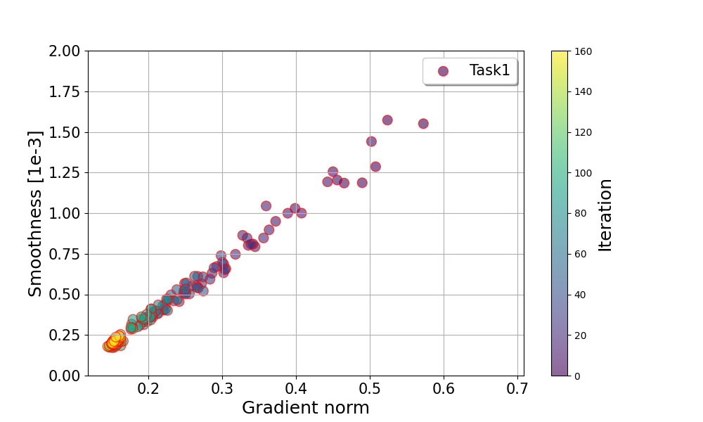
Figure 1: Multi-task learning on Cityscapes dataset.

Figure 2: Gradient norm vs smoothness

7 Conclusion

In this paper, we investigate the multi-objective problem with a more challenging, relaxed and realistic $\ell$-smooth assumption. We propose the first efficient MOO algorithm GSMGrad and its stochastic variant SGSMGrad for this problem. We provide the convergence guarantee for both algorithms to find an $\epsilon$-accurate Pareto stationary point with $\epsilon$-level average/iteration-wise CA distance. Extensive experiments are conducted to validate our theoretical results.

Appendix A Experimental details

A.1 Relation between gradient norms and the local smoothness

We show the relation between local smoothness and gradient norms of each task in this part. Both results demonstrate a positive correlation between them, which further substantiates the necessity of our analysis.

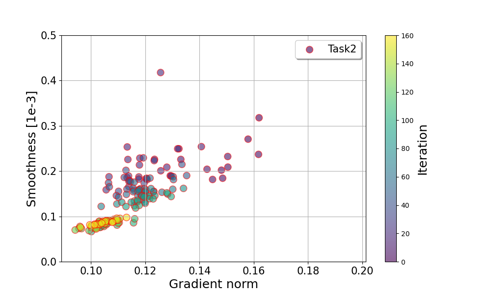
Figure 3: Local smoothness constant vs. Gradient norm on training SegNet on CityScapes dataset of each task. Task 1 on the left and Task 2 on the right.

A.2 Running time comparison between GSMGrad and GSMGrad-FA

We compare the average running time of the proposed algorithms, GSMGrad and GSMGrad-FA. The time in Table 1 is an average of the total running time over epochs (in minutes). The result solidifies the advantage of the fast approximation.

Method	Average running time
GSMGrad	2.93
GSMGrad-FA	1.93

Table 1: Average running time comparison between GSMGrad and GSMGrad-FA.

A.3 Implementation details

Multi-task learning on Cityscapes dataset. Following the experiment setup in [32], we train our method for 200 epochs, using SGD optimizers for both model parameters and weights, and the batch size for Cityscapes is 8. We compute the averaged test performance over the last 10 epochs as the final performance measure. We fix the $\beta=0.5$ and do a grid search on hyperparameters including $N\in[10,20,40,50],\alpha\in[0.0001,0.0002,0.0005,0.001]$, and $\rho\in[0.01,0.05,0.1,0.2,0.5,0.6,0.7,0.8,0.9,1]$ and choose the best result from them. It turns out our best performance of GSMGrad is based on the choice that $N=40,\alpha=0.0005,\beta=0.5$, and $\rho=0.5$. The choice of hyperparameters for GSMGrad-FA turns out to be the same as that for GSMGrad. All experiments are run on NVIDIA RTX A6000.

$\Delta m\%$ reflects the average per-task performance drop versus the single-task (STL) baseline $b$ to assess method $m$. We calculate it by the following equation

$$\Delta m\%=\frac{1}{K}\sum_{k=1}^{K}(-1)^{l_{k}}(M_{m,k}-M_{b,k})/M_{b,k}\times 100,$$

where $K$ is the number of metrics, $M_{b,k}$ is the value of metric $M_{k}$ obtained by baseline $b$, and $M_{m,k}$ obtained by the compared method $m$. $l_{k}=1$ if the evaluation metric $M_{k}$ on task $k$ prefers a higher value and $0$ otherwise.

Generalized smoothness illustration. To illustrate the relation between gradient norms and local smoothness, we run SGD on each task separately without the warm start process. Since there is no weight update process, we only need to choose $\alpha=0.0005$ for both tasks.

Appendix B Algorithm

We show our GSMGrad with Fast Approximation (GSMGrad-FA):

Algorithm 4 GSMGrad with Fast Approximation (GSMGrad-FA)

1:  Initialize: model parameters $x_{0}$, weights $w_{0}$ and a constant $\rho$

2:  $w_{0}$=Warm-start($w_{0}$, $x_{0}$, $\rho$)

3:  for $t=0,1,...,T-1$ do

4:     $x_{t+1}=x_{t}-\alpha\nabla F(x_{t})w_{t}$

5:     Update $w_{t}$ according to eq. 8

6:  end for

Appendix C Detailed Proofs for Average CA Distance

C.1 Formal version and proof of Theorem 1

Let $c_{1}>0,c_{2}>0$, $c_{3}\geq 0$ and $F>0$ be some constants such that

$$\Delta+c_{1}+{c_{2}}+c_{3}\leq F.$$ (10)

Define $M=\sup\{z\geq 0|\varphi(z)\leq F\}$. We then have the following convergence rate for Algorithm 1 without warm start:

Theorem 7.

Suppose Assumptions 1 and 2 are satisfied, and we choose constant step sizes that $\beta\leq\frac{1}{4KM^{2}},\alpha\leq\min\left(c_{1}\beta,\frac{1}{2\ell(M+1)},\frac{1}{M\ell(M+1)}\right),T\geq\max\left(\frac{10\Delta}{\alpha\epsilon^{2}},\frac{10}{\epsilon^{2}\beta}\right)\sim\Theta(\epsilon^{-2})$, and $\rho\leq\min\left(\frac{\epsilon^{2}}{20},\sqrt{\frac{\epsilon^{2}}{10\beta}},\frac{c_{2}}{2T\alpha},\sqrt{\frac{c_{3}}{T\alpha\beta}}\right)\sim\mathcal{O}(\epsilon^{2})$. We have that

$$\frac{1}{T}\sum_{t=0}^{T-1}\|\nabla F(x_{t})w_{t}\|^{2}\leq\epsilon^{2}.$$ (11)

Proof.

Compared with the standard $L$-smoothness, the generalized smoothness is more challenging to address due to the unbounded Lipschitz constant. Lemma 2 demonstrates that a bounded function value implies a bounded gradient norm, which further implies a bounded Lipschitz constant. In the following, we solve the unbounded Lipschitz constant problem by showing that the function value is bounded with the parameters selected in Theorem 1. We prove that for any $i\in K$ and $t\leq T$ we have that $f_{i}(x_{t})-f_{i}^{*}\leq F$ by induction.

Base Case: since all $c_{1},c_{2},c_{3},M$ are non-negative, according to (10) we have that $f_{i}(x_{0})-f_{i}^{*}\leq\Delta\leq F$ holds for any $i\in[K]$.

Induction step: assume that for any $i\in[K]$ and $t\leq k<T$, we have that $f_{i}(x_{t})-f_{i}^{*}\leq F$ holds. We then prove that $f_{i}(x_{k+1})-f_{i}^{*}\leq F$ holds for any $i\in[K]$.

For $f_{i}(x_{t})-f_{i}^{*}\leq F$, based on the monotonicity shown in Lemma 2, we have that $\|\nabla f_{i}(x_{t})\|\leq M$. From assumption 2, we have that $f_{i}(x)$ is $\left(\frac{1}{\ell(\|\nabla f_{i}(x))\|+1)},\ell(\|\nabla f_{i}(x)\|+1)\right)$-smooth by setting $a=1$. For any $t\leq k$, we have that

$$\|x_{t+1}-x_{t}\|=\alpha\|\nabla F(x_{t})w_{t}\|\leq\alpha M\leq\frac{1}{\ell(M+1)}\leq\frac{1}{\ell(\|\nabla f_{i}(x_{t})\|+1)},$$

where the second inequality is due to $\alpha\leq\frac{1}{M\ell(M+1)}$ and the last inequality is due to $\|\nabla f_{i}(x_{t})\|\leq M$. Based on Assumption 2, Definition 2 and Lemma 3.3 in [21], we have the following descent lemma:

$$f_{i}(x_{t+1}) \leq f_{i}(x_{t})-\alpha\langle\nabla f_{i}(x_{t}),\nabla F(x_{t})w_{t}\rangle+\frac{\ell(\|\nabla f_{i}(x_{t})\|+1)}{2}\alpha^{2}\|\nabla F(x_{t})w_{t}\|^{2}$$

$$\leq f_{i}(x_{t})-\alpha\langle\nabla f_{i}(x_{t}),\nabla F(x_{t})w_{t}\rangle+\frac{\ell(M+1)}{2}\alpha^{2}\|\nabla F(x_{t})w_{t}\|^{2}.$$

As a result, for any $w\in\mathcal{W}$, we have that

$$F(x_{t+1})w\leq F(x_{t})w-\alpha\langle\nabla F(x_{t})w,\nabla F(x_{t})w_{t}\rangle+\frac{\ell(M+1)}{2}\alpha^{2}\|\nabla F(x_{t})w_{t}\|^{2}.$$ (12)

Based on the update process of $w$, we have that

$$w_{t+1} =\Pi_{\mathcal{W}}\Big{(}w_{t}-\beta\Big{(}\nabla F(x_{t})^{\top}\nabla F(x_{t})w_{t}+\rho w_{t}\Big{)}\Big{)}.$$

It then follows that

$$\|w_{t+1}-w\|^{2}$$

$$=\Big{\|}\Pi_{\mathcal{W}}\Big{(}w_{t}-\beta\Big{(}\nabla F(x_{t})^{\top}\nabla F(x_{t})w_{t}+\rho w_{t}\Big{)}\Big{)}-w\Big{\|}^{2}$$

$$\leq\Big{\|}\Big{(}w_{t}-\beta\Big{(}\nabla F(x_{t})^{\top}\nabla F(x_{t})w_{t}+\rho w_{t}\Big{)}\Big{)}-w\Big{\|}^{2}$$

$$=\|w_{t}-w\|^{2}-2\beta\left\langle w_{t}-w,(\nabla F(x_{t})^{\top}\nabla F(x_{t})+\rho I)w_{t}\right\rangle$$

$$+\beta^{2}\left\|(\nabla F(x_{t})^{\top}\nabla F(x_{t})+\rho I)w_{t}\right\|^{2},$$

where the inequality is due to the non-expansiveness of projection. By rearranging the above inequality, we have that

$$\langle w_{t}-w,\nabla F(x_{t})^{\top}\nabla F(x_{t})w_{t}\rangle$$

$$\leq\frac{1}{2\beta}\left(\|w_{t}-w\|^{2}-\|w_{t+1}-w\|^{2}\right)+2\rho+\beta KM^{2}\|\nabla F(x_{t})w_{t}\|^{2}+\beta\rho^{2}.$$ (13)

Plug (C.1) into (12), and we can show that

$$F(x_{t+1})w-F(x_{t})w$$

$$\leq-\alpha\|\nabla F(x_{t})w_{t}\|^{2}+\frac{\ell(M+1)}{2}\alpha^{2}\|\nabla F(x_{t})w_{t}\|^{2}$$

$$+\frac{\alpha}{2\beta}\left(\|w_{t}-w\|^{2}-\|w_{t+1}-w\|^{2}\right)+\alpha\beta KM^{2}\|\nabla F(x_{t})w_{t}\|^{2}+\alpha\beta\rho^{2}+2\alpha\rho.$$ (14)

Taking sums of (C.1) from $t=0$ to $k$, for any $w\in\mathcal{W}$ we have that

$$F(x_{k+1})w-F(x_{0})w$$

$$\leq-\sum_{t=0}^{k}\alpha\|\nabla F(x_{t})w_{t}\|^{2}+\sum_{t=0}^{k}\left(\frac{\ell(M+1)}{2}\alpha^{2}+\alpha\beta KM^{2}\right)\|\nabla F(x_{t})w_{t}\|^{2}$$

$$+\frac{\alpha}{2\beta}\|w_{0}-w\|^{2}+T\alpha\beta\rho^{2}+2T\alpha\rho$$

$$\leq\frac{\alpha}{2\beta}\|w_{0}-w\|^{2}+T\alpha\beta\rho^{2}+2T\alpha\rho,$$ (15)

where the first inequality is due to $k<T$ and the last inequality is due to that $\alpha\leq\frac{1}{2\ell(M+1)}$ and $\beta KM^{2}\leq{\frac{1}{4}}$. Thus for any $i\in[K]$ it can be shown that

$$f_{i}(x_{t+1})-f_{i}^{*}\leq f_{i}(x_{0})-f_{i}^{*}+\frac{\alpha}{\beta}+T\alpha\beta\rho^{2}+2T\alpha\rho\leq F,$$

since we have that $\frac{\alpha}{\beta}\leq c_{1},T\alpha\beta\rho^{2}\leq c_{3}$ and $2T\alpha\rho\leq c_{2}$. Now we finish the induction step and can show that $f_{i}(x_{k+1})-f_{i}^{*}\leq F$ and (C.1) hold for all $k<T$ and $i\in[K]$.

Specifically, for $\alpha<\frac{1}{2\ell(M+1)},\beta\leq\frac{1}{4KM^{2}}$, according to (C.1), for $k=T-1$ we have that

$$\frac{1}{T}\sum_{t=0}^{T-1}\|\nabla F(x_{t})w_{t}\|^{2}\leq\frac{2(F(x_{0})w-F^{*}w)}{\alpha T}+\frac{2}{\beta T}+2\beta\rho^{2}+4\rho\leq\epsilon^{2},$$

which completes our proof. ∎

Lemma 2.

(Lemma 3.5 in [21]) If a function $f$ is $\ell$-smooth, we have that

$$\varphi(\|\nabla f(x)\|)=\frac{\|\nabla f(x)\|^{2}}{2\ell(2\|\nabla f(x)\|)}\leq f(x)-f^{*}.$$ (16)

C.2 Proof of Corollary 1

Proof.

Recall that

$$\|\nabla F(x_{t})w_{t}-\nabla F(x_{t})w_{t}^{*}\|^{2}\leq\|\nabla F(x_{t})w_{t}\|^{2}-\|\nabla F(x_{t})w_{t}^{*}\|^{2}\leq\|\nabla F(x_{t})w_{t}\|^{2},$$

where the first inequality follows from the optimal condition. Then we have

$$\frac{1}{T}\sum_{t=0}^{T-1}\|\nabla F(x_{t})w_{t}-\nabla F(x_{t})w_{t}\|^{2}\leq\frac{1}{T}\sum_{t=0}^{T-1}|\|\nabla F(x_{t})w_{t}\|^{2}=\mathcal{O}(\epsilon^{2}),$$

where we follow the same setting in Theorem 1. The proof is complete. ∎

C.3 Formal Version and Its Proof of Theorem 2

Let $c_{1}>0,c_{2}>0,c_{3}>0,c_{4}>0,c_{5}>0,c_{6}>0$ be some constants. Let $F>0$ and $0<\delta\leq\frac{1}{2}$ be some constants such that

$$F\geq\frac{8(\Delta+c_{1}+c_{2}+c_{3}+c_{4}+c_{5}+c_{6})}{\delta},$$

where $\Delta=\max_{i\in[d]}\{f_{i}(x_{0})-f^{*}\}$. Let $L_{0}>0,L_{1}>0,b_{1}>0,b_{2}>0,b_{3}>0$ be some constants.

For $\alpha\leq\min\{\frac{\ell(M+1)}{2\max(1,M)},c_{1}\beta,\rho\min\left\{\frac{1}{4L_{0}^{2}\ell(M+1)^{2}},\frac{b_{1}^{2}}{(3M\sqrt{K}L_{0}+M\sqrt{K}L_{1})^{2}},\frac{b_{2}}{\ell(M+1)L_{0}^{2}}\right\},\frac{c_{2}}{\sqrt{2T}M(3\sigma+\sigma^{2}),},\\ \frac{\sqrt{c_{3}}}{\sqrt{\ell(M+1)\sigma^{2}T}},\frac{\delta\epsilon^{2}}{48\sigma^{2}\ell(M+1)}\}$,

$\beta\leq\min\{\frac{c_{4}}{4K\alpha T(M^{2}+\sigma^{2})^{2}},\frac{\delta\epsilon^{2}}{192K(M^{2}+\sigma^{2})^{2}},\frac{b_{3}\rho}{8KM^{2}L_{0}^{2}+4KL_{1}^{2}}\},\\ \rho\leq\min\{\frac{c_{5}}{\alpha T},{\frac{\sqrt{c_{6}}}{\sqrt{\alpha\beta T}}},\frac{\delta\epsilon^{2}}{48},\sqrt{\frac{\delta\epsilon^{2}}{48\beta}},\frac{\delta L_{0}^{2}}{24K\sigma^{2}\alpha T},\frac{\delta L_{1}^{2}}{8K^{2}\sigma^{4}\alpha T}\}$,
and $T\geq\max\{\frac{48\Delta+48c_{1}}{\delta\alpha\epsilon^{2}},\frac{4608M^{2}(3\sigma+\sigma^{2})^{2}}{\delta^{2}\epsilon^{4}}\}$ such that

$$b_{1}+b_{2}+c_{1}+\alpha\rho(1+\beta\rho)+4\alpha\beta KM^{4}\leq\frac{F}{2}.$$ (17)

Define the following random variables

$$\tau_{1}=\min\{t|\exists i\in[K],f_{i}(x_{t+1})-f_{i}^{*}>F\}\wedge T,$$

$$\tau_{2}=\min\{t|\exists i\in[K],j\in[3],\|\varepsilon_{t,j,i}\|>\frac{L_{0}}{\sqrt{\alpha\rho}}\}\wedge T,$$

$$\tau_{3}=\min\{t|\exists i,j\in[K],\|\varepsilon_{t,2,i}\|\|\varepsilon_{t,3,j}\|>\frac{L_{1}}{\sqrt{\alpha\rho}}\}\wedge T,$$

$$\tau=\min\{\tau_{1},\tau_{2},\tau_{3}\}.$$

We then have the following theorem:

Theorem 8.

If Assumptions 1, 2 and 3 hold, with the parameters selected above, we have that

$$\frac{1}{T}\sum_{t=0}^{T-1}\|\nabla F(x_{t})w_{t}\|^{2}\leq\epsilon^{2},$$

with the probability at least $1-\delta$.

Proof.

Small probability of the event $\{\tau<T\}$.

We first show that the probability of the event $\{\tau<T\}$ is small: $\mathbb{P}(\tau<T)\leq\delta$. Note that

$$\{\tau<T\}=\{\tau_{2}<T\}\cup\{\tau_{3}<T\}\cup\{\tau_{1}<T,\tau_{2}=T,\tau_{3}=T\}.$$

For any $i\in[K],j\in[3]$, we have that

$$\mathbb{P}(\|\varepsilon_{t,j,i}\|>\frac{L_{0}}{\sqrt{\alpha\rho}})=\mathbb{P}(\|\varepsilon_{t,j,i}\|^{2}>\frac{L_{0}^{2}}{{\alpha\rho}})\leq\frac{\sigma^{2}{\alpha\rho}}{L_{0}^{2}},$$

where the last inequality is due to Chebyshev’s inequality. Based on the union bound, we have that

$$\mathbb{P}(\{\tau_{2}<T\})\leq\sum_{t=0}^{T-1}\sum_{j=1}^{K}\sum_{i=1}^{3}\mathbb{P}(\|\varepsilon_{t,j,i}\|>\frac{L_{0}}{\sqrt{\alpha\rho}})\leq\frac{3K\sigma^{2}{\alpha\rho}T}{L_{0}^{2}}\leq\frac{\delta}{8}$$ (18)

since $\rho\leq\frac{\delta L_{0}^{2}}{24K\sigma^{2}\alpha T}$. Similarly, we have that

$$\mathbb{P}(\|\varepsilon_{t,2,i}\|\|\varepsilon_{t,3,i}\|>\frac{L_{1}}{\sqrt{\alpha\rho}})=\mathbb{P}(\|\varepsilon_{t,2,i}\|^{2}\|\varepsilon_{t,3,i}\|^{2}>\frac{L_{1}^{2}}{{\alpha\rho}})\leq\frac{\sigma^{4}{\alpha\rho}}{L_{1}^{2}}.$$

It follows that

$$\mathbb{P}(\{\tau_{3}<T\})\leq\sum_{t=0}^{T-1}\sum_{i=1}^{K}\sum_{j=1}^{K}\mathbb{P}(\|\varepsilon_{t,2,i}\|\|\varepsilon_{t,3,i}\|>\frac{L_{1}}{\sqrt{\alpha\rho}})\leq\frac{K^{2}\sigma^{4}{\alpha\rho}T}{L_{1}^{2}}\leq\frac{\delta}{8}.$$ (19)

We then bound the probability of the event $\{\tau_{1}<T,\tau_{2}=T,\tau_{3}=T\}$. Since $\tau=\tau_{1}<T,$ we have that for some $i\in[K]$, $f_{i}(x_{\tau+1})-f_{i}^{*}>F$.

According to (C.4) shown in Lemma 1, for any $i\in[K]$ and $t=\tau$ we have that

$$f_{i}(x_{\tau+1})-f_{i}(x_{\tau}) \leq\alpha\|\nabla F(x_{\tau})w\|\|\varepsilon_{t,1}w_{t}\|+{\ell(M+1)}\alpha^{2}\|\varepsilon_{t,1}w_{t}\|^{2}+\frac{\alpha}{\beta}+\alpha\rho+\alpha\beta\rho^{2}$$

$$+\alpha M\|\varepsilon_{t,2}\|+\alpha M\|\varepsilon_{t,3}\|+\alpha\|\varepsilon_{t,2}^{\top}\varepsilon_{t,3}w_{t}\|$$

$$+4\alpha\beta KM^{4}+4\alpha\beta M^{2}\|\varepsilon_{t,2}\|^{2}+4\alpha\beta M^{2}\|\varepsilon_{t,3}\|^{2}+4\alpha\beta\|\varepsilon_{t,2}^{\top}\varepsilon_{t,3}w_{t}\|^{2}$$

$$\leq\alpha M\frac{L_{0}}{\sqrt{\alpha\rho}}+{\ell(M+1)}\alpha\frac{L_{0}^{2}}{{\rho}}+\frac{\alpha}{\beta}+\alpha\rho+\alpha\beta\rho^{2}$$

$$+\alpha M\frac{\sqrt{K}L_{0}}{\sqrt{\alpha\rho}}+\alpha M\frac{\sqrt{K}L_{0}}{\sqrt{\alpha\rho}}+\alpha M\frac{\sqrt{K}L_{1}}{\sqrt{\alpha\rho}}$$

$$+4\alpha\beta KM^{4}+4\alpha\beta M^{2}\frac{KL_{0}^{2}}{{\alpha\rho}}+4\alpha\beta M^{2}\frac{KL_{0}^{2}}{{\alpha\rho}}+4\alpha\beta\frac{KL_{1}^{2}}{{\alpha\rho}}$$

$$\leq b_{1}+b_{2}+b_{3}+c_{1}+\alpha\rho(1+\beta\rho)+4\alpha\beta KM^{4}$$

$$\leq\frac{F}{2},$$

where the first inequality is due to that $\tau_{2}=\tau_{3}=T$, and the second one is due to $\frac{\beta}{\rho}\leq\frac{b_{3}}{8KM^{2}L_{0}^{2}+4KL_{1}^{2}}$ and $\frac{\alpha}{\rho}\leq\min\left\{\frac{b_{1}^{2}}{(3M\sqrt{K}L_{0}+M\sqrt{K}L_{1})^{2}},\frac{b_{2}}{\ell(M+1)L_{0}^{2}}\right\}$.

However, for some $i\in[K]$, $f_{i}(x_{\tau+1})-f_{i}^{*}>F$. Thus for this task, we have that

$$f_{i}(x_{\tau})-f_{i}^{*}\leq\frac{F}{2}.$$

According to Lemma 1, we have that

$$\mathbb{E}[f_{i}(x_{\tau})-f_{i}^{*}]\leq\frac{\delta}{8}.$$

Based on Markov inequality, it follows that

$$\mathbb{P}\left(f_{i}(x_{\tau})-f_{i}^{*}\leq\frac{F}{2}\right)\leq\frac{\mathbb{E}[f_{i}(x_{\tau})-f_{i}^{*}]}{F/2}\leq\frac{\delta}{4},$$ (20)

which indicates that $\mathbb{P}(\tau_{1}<T,\tau_{2}=T,\tau_{3}=T)\leq\frac{\delta}{4}$. It follows that $\mathbb{P}(\tau<T)\leq\frac{\delta}{2}$.

Convergence of $\frac{1}{T}\mathbb{E}\left[\sum_{t=0}^{T-1}\|\nabla F(x_{t})w_{t}\|^{2}\Big{|}\tau=T\right]$. Based on (C.4) in Lemma 1, we have that

$$\frac{1}{T}\mathbb{E}\left[\sum_{t=0}^{T-1}\|\nabla F(x_{t})w_{t}\|^{2}\Big{|}\tau=T\right]$$

$$\leq\frac{1}{T}\frac{1}{\mathbb{P}(\tau=T)}\mathbb{E}\left[\sum_{t=0}^{\tau-1}\|\nabla F(x_{t})w_{t}\|^{2}\right]$$

$$\leq\frac{4F(x_{0})w-4F^{*}w+\frac{4\alpha}{\beta}}{\alpha T}+\frac{4\sqrt{2}M(3\sigma+\sigma^{2})}{\sqrt{T}}+4\alpha\sigma^{2}\ell(M+1)+4\rho$$

$$+4\beta\rho^{2}+16\beta KM^{4}+32\beta KM^{2}\sigma^{2}+16\beta K\sigma^{4}$$

$$\leq\frac{\delta}{2}\epsilon^{2},$$

where the second inequality is due to $\delta<\frac{1}{2}$ and the last inequality is due to our selection of parameters. As a result, we have that

$$\mathbb{P}\left(\frac{1}{T}\sum_{t=0}^{T-1}\|\nabla F(x_{t})w_{t}\|^{2}>\epsilon^{2}\Big{|}\tau=T\right)\leq\frac{\mathbb{E}\left[\frac{1}{T}\sum_{t=0}^{T-1}\|\nabla F(x_{t})w_{t}\|^{2}\geq\epsilon^{2}\Big{|}\tau=T\right]}{\epsilon^{2}}\leq\frac{\delta}{2},$$ (21)

where the first probability is due to Markov inequality. Thus we have that

$$\mathbb{P}\left(\frac{1}{T}\sum_{t=0}^{T-1}\|\nabla F(x_{t})w_{t}\|^{2}\leq\epsilon^{2}\right)$$

$$\geq 1-\mathbb{P}\left(\tau<T\right)-\mathbb{P}\left(\frac{1}{T}\sum_{t=0}^{T-1}\|\nabla F(x_{t})w_{t}\|^{2}>\epsilon^{2}\Big{|}\tau=T\right)\mathbb{P}\left(\tau=T\right)$$

$$\geq 1-\delta,$$

where the last inequality is due to (18), (19), (20), and (21). This completes the proof. ∎

C.4 Proof of Lemma 1

Proof.

For all $i\in[K],t\leq\tau$, we have $f_{i}(x_{t})-f_{i}^{*}\leq F$ which further implies that $\|\nabla f_{i}(x_{t})\|\leq M$. Moreover, we have that for any $t\leq\tau$ and $i\in[K]$,

$$\|x_{t+1}-x_{t}\|\leq\alpha\|\nabla G_{1}(x_{t})w_{t}\|\leq\alpha(\|\nabla F(x_{t})w_{t}\|+\|\varepsilon_{t,1}w_{t}\|)\leq\alpha\left(M+\frac{L_{0}}{\sqrt{\alpha\rho}}\right)\leq\frac{1}{\ell(M+1)}.$$

Since $f_{i}(x)$ is $\left(\frac{1}{\ell(\|\nabla f_{i}(x))\|+1)},\ell(\|\nabla f_{i}(x)\|+1)\right)$-smooth, it follows that

$$f_{i}(x_{t+1})-f_{i}(x_{t})\leq-\alpha\langle\nabla f_{i}(x_{t}),\nabla G_{1}(x_{t})w_{t}\rangle+\frac{\ell(\|\nabla f_{i}(x_{t})\|+1)}{2}\alpha^{2}\|\nabla G_{1}(x_{t})w_{t}\|^{2}.$$

As a result, for any $w\in\mathcal{W}$, we have that

$$F(x_{t+1})w \leq F(x_{t})w-\alpha\langle\nabla F(x_{t})w,\nabla G_{1}(x_{t})w_{t}\rangle+\frac{\ell(M+1)}{2}\alpha^{2}\|\nabla G_{1}(x_{t})w_{t}\|^{2}$$

$$\leq F(x_{t})w-\alpha\langle\nabla F(x_{t})w,\nabla F(x_{t})w_{t}\rangle+\alpha\langle\nabla F(x_{t})w,\varepsilon_{t,1}w_{t}\rangle$$

$$+{\ell(M+1)}\alpha^{2}\|\nabla F(x_{t})w_{t}\|^{2}+{\ell(M+1)}\alpha^{2}\|\varepsilon_{t,1}w_{t}\|^{2}$$ (22)

Based on the update process of $w$, we have that

$$\|w_{t+1}-w\|^{2}$$

$$=\|\Pi_{\mathcal{W}}\big{(}w_{t}-\beta[{\nabla G_{2}(x_{t})^{\top}\nabla G_{3}(x_{t})w_{t}}+\rho w_{t}]\big{)}-w\|^{2}$$

$$\leq\|\big{(}w_{t}-\beta[{\nabla G_{2}(x_{t})^{\top}\nabla G_{3}(x_{t})w_{t}}+\rho w_{t}]\big{)}-w\|^{2}$$

$$=\|w_{t}-w\|^{2}-2\beta\langle w_{t}-w,(\nabla G_{2}(x_{t})^{\top}\nabla G_{3}(x_{t})+\rho)w_{t}\rangle$$

$$+\beta^{2}\|(\nabla G_{2}(x_{t})^{\top}\nabla G_{3}(x_{t})+\rho)w_{t}\|^{2},$$

where the inequality follows from the non-expansiveness of projection. It follows that

$$2\beta\langle w_{t}-w,\nabla F(x_{t})^{\top}\nabla F(x_{t})w_{t}\rangle$$

$$\leq\left(\|w_{t}-w\|^{2}-\|w_{t+1}-w\|^{2}\right)+2\beta\rho+2\beta^{2}\rho^{2}$$

$$+2\beta\left\langle w_{t}-w,\varepsilon_{t,2}^{\top}\nabla F(x_{t})w_{t}+\nabla F(x_{t})^{\top}\varepsilon_{t,3}w_{t}-\varepsilon_{t,2}^{\top}\varepsilon_{t,3}w_{t}\right\rangle$$

$$+2\beta^{2}\|\nabla F(x_{t})^{\top}\nabla F(x_{t})w_{t}-\varepsilon_{t,2}^{\top}\nabla F(x_{t})w_{t}-\nabla F(x_{t})^{\top}\varepsilon_{t,3}w_{t}+\varepsilon_{t,2}^{\top}\varepsilon_{t,3}w_{t}\|^{2}$$

$$\leq\left(\|w_{t}-w\|^{2}-\|w_{t+1}-w\|^{2}\right)+2\beta\rho+2\beta^{2}\rho^{2}$$

$$+2\beta\left\langle w_{t}-w,\varepsilon_{t,2}^{\top}\nabla F(x_{t})w_{t}+\nabla F(x_{t})^{\top}\varepsilon_{t,3}w_{t}-\varepsilon_{t,2}^{\top}\varepsilon_{t,3}w_{t}\right\rangle$$

$$+8\beta^{2}KM^{4}+8\beta^{2}M^{2}\|\varepsilon_{t,2}\|^{2}+8\beta^{2}M^{2}\|\varepsilon_{t,3}\|^{2}+8\beta^{2}\|\varepsilon_{t,2}^{\top}\varepsilon_{t,3}w_{t}\|^{2}.$$ (23)

Combine (C.4) and (C.4), and we can get that

$$F(x_{t+1})w-F(x_{t})w \leq-\alpha\|\nabla F(x_{t})w_{t}\|^{2}+\alpha\langle\nabla F(x_{t})w,\varepsilon_{t,1}w_{t}\rangle$$

$$+{\ell(M+1)}\alpha^{2}\|\nabla F(x_{t})w_{t}\|^{2}+{\ell(M+1)}\alpha^{2}\|\varepsilon_{t,1}w_{t}\|^{2}$$

$$+\frac{\alpha}{2\beta}\left(\|w_{t}-w\|^{2}-\|w_{t+1}-w\|^{2}\right)+\alpha\rho+\alpha\beta\rho^{2}$$

$$+\alpha\left\langle w_{t}-w,\varepsilon_{t,2}^{\top}\nabla F(x_{t})w_{t}+\nabla F(x_{t})w_{t}^{\top}\varepsilon_{t,3}-\varepsilon_{t,2}^{\top}\varepsilon_{t,3}w_{t}\right\rangle$$

$$+4\alpha\beta KM^{4}+4\alpha\beta M^{2}\|\varepsilon_{t,2}\|^{2}+4\alpha\beta M^{2}\|\varepsilon_{t,3}\|^{2}+4\alpha\beta\|\varepsilon_{t,2}^{\top}\varepsilon_{t,3}w_{t}\|^{2}.$$ (24)

Taking expectation and sum up (C.4) from $t=0$ to $\tau-1$, we have that

$$\mathbb{E}[F(x_{\tau})w]-F(x_{0})w \leq-\frac{\alpha}{2}\mathbb{E}\left[\sum_{t=0}^{\tau-1}\|\nabla F(x_{t})w_{t}\|^{2}\right]+\alpha\mathbb{E}\left[\sum_{t=0}^{\tau-1}\langle\nabla F(x_{t})w,\varepsilon_{t,1}w_{t}\rangle\right]$$

$$+\alpha\mathbb{E}\left[\sum_{t=0}^{\tau-1}\left\langle w_{t}-w,\varepsilon_{t,2}^{\top}\nabla F(x_{t})w_{t}+\nabla F(x_{t})w_{t}^{\top}\varepsilon_{t,3}-\varepsilon_{t,2}^{\top}\varepsilon_{t,3}w_{t}\right\rangle\right]$$

$$+{\ell(M+1)}\alpha^{2}\mathbb{E}\left[\sum_{t=0}^{\tau-1}\|\varepsilon_{t,1}w_{t}\|^{2}\right]+\frac{\alpha}{2\beta}\|w_{0}-w\|^{2}+\alpha\rho T+\alpha\beta\rho^{2}T$$

$$+4\alpha\beta KM^{4}T+4\alpha\beta M^{2}\mathbb{E}\left[\sum_{t=0}^{\tau-1}\|\varepsilon_{t,2}\|^{2}\right]$$

$$+4\alpha\beta M^{2}\mathbb{E}\left[\sum_{t=0}^{\tau-1}\|\varepsilon_{t,3}\|^{2}\right]+4\alpha\beta\mathbb{E}\left[\sum_{t=0}^{\tau-1}\|\varepsilon_{t,2}^{\top}\varepsilon_{t,3}w_{t}\|^{2}\right]$$

$$\leq-\frac{\alpha}{2}\mathbb{E}\left[\sum_{t=0}^{\tau-1}\|\nabla F(x_{t})w_{t}\|^{2}\right]+\alpha\mathbb{E}\left[\sum_{t=0}^{\tau-1}\langle\nabla F(x_{t})w,\varepsilon_{t,1}w_{t}\rangle\right]$$

$$+\alpha\mathbb{E}\left[\sum_{t=0}^{\tau-1}\left\langle w_{t}-w,\varepsilon_{t,2}^{\top}\nabla F(x_{t})w_{t}+\nabla F(x_{t})w_{t}^{\top}\varepsilon_{t,3}-\varepsilon_{t,2}^{\top}\varepsilon_{t,3}w_{t}\right\rangle\right]$$

$$+{\ell(M+1)}\alpha^{2}T\sigma^{2}+\frac{\alpha}{\beta}+\alpha\rho T+\alpha\beta\rho^{2}T$$

$$+4\alpha\beta KM^{4}T+4\alpha\beta KM^{2}T\sigma^{2}$$

$$+4\alpha\beta KM^{2}T\sigma^{2}+4\alpha\beta TK\sigma^{4},$$ (25)

where the last inequality is due to that $\tau\leq T$ and for any $i\in[K],j\in[3]$, $\mathbb{E}\left[\sum_{t=0}^{\tau-1}\|\varepsilon_{t,j,i}\|^{2}\right]\leq\mathbb{E}\left[\sum_{t=0}^{T-1}\|\varepsilon_{t,j,i}\|^{2}\right]\leq TK\sigma^{2}$. By the optional stopping theorem, we have that

$$\mathbb{E}\left[\sum_{t=0}^{\tau}\langle\nabla F(x_{t})w,\varepsilon_{t,1}w_{t}\rangle\right]=0,$$

which further implies that

$$\mathbb{E}\left[\sum_{t=0}^{\tau-1}\langle\nabla F(x_{t})w,\varepsilon_{t,1}w_{t}\rangle\right] =-\mathbb{E}[\langle\nabla F(x_{\tau})w,\varepsilon_{\tau,1}w_{\tau}\rangle]$$

$$\leq\mathbb{E}[M\|\varepsilon_{\tau,1}w_{\tau}\|]\leq M\sqrt{\mathbb{E}[\|\varepsilon_{\tau,1}w_{\tau}\|^{2}]}$$

$$\leq M\sqrt{\mathbb{E}\left[\sum_{t=0}^{T}\|\varepsilon_{t,1}w_{t}\|^{2}\right]}\leq M\sigma\sqrt{T+1}$$

$$\leq\sqrt{2}M\sigma\sqrt{T}.$$ (26)

Similarly, we have $\mathbb{E}\left[\sum_{t=0}^{\tau-1}\langle\nabla F(x_{t})w,\varepsilon_{t,2}w_{t}\rangle\right]\leq\sqrt{2}M\sigma\sqrt{T}$, $\mathbb{E}\left[\sum_{t=0}^{\tau-1}\langle\nabla F(x_{t})w,\varepsilon_{t,3}w_{t}\rangle\right]\leq\sqrt{2}M\sigma\sqrt{T}$ and $\mathbb{E}\left[\sum_{t=0}^{\tau-1}\langle\nabla F(x_{t})w,\varepsilon_{t,2}^{\top}\varepsilon_{t,3}w_{t}\rangle\right]\leq\sqrt{2K}M\sigma^{2}\sqrt{T}$.

Based on (C.4) and (C.4), we have that

$$\mathbb{E}[F(x_{\tau})w]-F^{*}w \leq F(x_{0})w-F^{*}w-\mathbb{E}\left[\sum_{t=0}^{\tau-1}\frac{\alpha}{2}\|\nabla F(x_{t})w_{t}\|^{2}\right]+\alpha\sqrt{2T}M(3\sigma+\sigma^{2})$$

$$+{\ell(M+1)}\alpha^{2}T\sigma^{2}+\frac{\alpha}{\beta}+\alpha\rho T+\alpha\beta\rho^{2}T$$

$$+4\alpha\beta KM^{4}T+4\alpha\beta KM^{2}T\sigma^{2}$$

$$+4\alpha\beta KM^{2}T\sigma^{2}+4\alpha\beta TK\sigma^{4}$$

$$\leq\frac{\delta F}{8}-\mathbb{E}\left[\sum_{t=0}^{\tau-1}\frac{\alpha}{2}\|\nabla F(x_{t})w_{t}\|^{2}\right],$$ (27)

which completes the proof. ∎

Appendix D Detailed Proofs for Iteration-wise CA Distance

We first provide some useful lemmas, which will be used in our main theorems.

Lemma 3 (Continuity of $w_{t,\rho}^{*}$).

Suppose Assumptions 1 and 2 are satisfied. If for any $i\in[K],\|\nabla f_{i}(x_{t})\|\leq M$ and $\|x_{t}-x_{t+1}\|\leq\frac{1}{\ell(M+1)}$, we have,

$$\|w_{\rho}^{*}(x_{t})-w_{\rho}^{*}(x_{t+1})\|\leq 2\rho^{-1}KM\ell(M+1)\|x_{t}-x_{t+1}\|=L_{w}\|x_{t}-x_{t+1}\|.$$

Proof.

We first define that $w_{Q,\rho}(x_{t})\in\mathcal{W}$ is the $Q$-th iterate of a function $J(w)=\frac{1}{2}\|\nabla F(x_{t})w\|^{2}+\frac{\rho}{2}\|w\|^{2}$ using projected gradient descent (PGD) with a constant step size $\beta$. The update rule is $w_{Q+1,\rho}(x_{t})=\Pi_{\mathcal{W}}\Big{(}\big{(}(1-\beta\rho)I-\beta\nabla F(x_{t})^{\top}\nabla F(x_{t})\big{)}w_{Q,\rho}(x_{t})\Big{)}$. By the non-expansiveness of projection, we have

$$\|w_{Q+1,\rho} (x_{t})-w_{Q+1,\rho}(x_{t+1})\|$$

$$\leq \|\big{(}(1-\beta\rho)I-\beta\nabla F(x_{t})^{\top}\nabla F(x_{t})\big{)}w_{Q,\rho}(x_{t})$$

$$-\big{(}(1-\beta\rho)I-\beta\nabla F^{\top}(x_{t+1})\nabla F(x_{t+1})\big{)}w_{Q,\rho}(x_{t+1})\|$$

$$\leq \|(1-\beta\rho)I-\beta\nabla F(x_{t})^{\top}\nabla F(x_{t})\|\|w_{Q,\rho}(x_{t})-w_{Q,\rho}(x_{t+1})\|$$

$$+\beta\|\big{(}\nabla F(x_{t})^{\top}\nabla F(x_{t})-\nabla F^{\top}(x_{t+1})\nabla F(x_{t+1})\big{)}w_{Q,\rho}(x_{t+1})\|$$

$$\leq (1-\beta\rho)\|w_{Q,\rho}(x_{t})-w_{Q,\rho}(x_{t+1})\|$$

$$+\beta\|\big{(}\nabla F(x_{t})^{\top}\nabla F(x_{t})-\nabla F^{\top}(x_{t+1})\nabla F(x_{t+1})\big{)}w_{Q,\rho}(x_{t+1})\|.$$ (28)

Since we set $w_{0,\rho}(x_{t})=w_{0,\rho}(x_{t+1})$ and $\|w_{Q,\rho}(x_{t+1})\|\leq 1$, telescoping the above inequality from $t=0,1,...,T-1$ gives,

$$\|w_{Q,\rho} (x_{t})-w_{Q,\rho}(x_{t+1})\|\leq\rho^{-1}\|\nabla F(x_{t})^{\top}\nabla F(x_{t})-\nabla F^{\top}(x_{t+1})\nabla F(x_{t+1})\|.$$ (29)

Then according to the Cauchy-Schwartz inequality, it follows that

$$\|w_{\rho}^{*}(x_{t})-w_{\rho}^{*}(x_{t+1})\|\leq \lim_{Q\rightarrow\infty}\big{(}\|w_{\rho}^{*}(x_{t})-w_{Q,\rho}(x_{t})\|+\|w_{\rho}^{*}(x_{t+1})-w_{Q,\rho}(x_{t+1})\|$$

$$+\|w_{Q,\rho}(x_{t})-w_{Q,\rho}(x_{t+1})\|\big{)}$$

$$\overset{(i)}{\leq} \lim_{Q\rightarrow\infty}\big{(}\|w_{\rho}^{*}(x_{t})-w_{Q,\rho}(x_{t})\|+\|w_{\rho}^{*}(x_{t+1})-w_{Q,\rho}(x_{t+1})\|\big{)}$$

$$+\rho^{-1}\|\nabla F(x_{t})^{\top}\nabla F(x_{t})-\nabla F^{\top}(x_{t+1})\nabla F(x_{t+1})\|$$

$$\overset{(ii)}{\leq} \lim_{Q\rightarrow\infty}2\sqrt{\frac{4}{\rho\beta Q}}+\rho^{-1}\|\nabla F(x_{t})^{\top}\nabla F(x_{t})-\nabla F^{\top}(x_{t+1})\nabla F(x_{t+1})\|,$$ (30)

where $(i)$ follows from eq. 29 and $(ii)$ follows from the convergence of PGD (Theorem 1.1, [4]) on $\rho$-strongly convex objectives that

$$\|w_{\rho}^{*}(x_{t})-w_{Q,\rho}(x_{t})\|^{2}\leq\frac{2}{\rho}\big{(}J(w_{\rho}^{*}(x_{t}))-J(w_{Q,\rho}(x_{t}))\big{)}\leq\frac{2}{\rho}\frac{\|w_{0,\rho}(x_{t})-w_{\rho}^{*}(x_{t})\|^{2}}{2\beta Q}\leq\frac{4}{\rho\beta Q}.$$

Then lemma 3 can be bounded by

$$\|w_{\rho}^{*}(x_{t})-w_{\rho}^{*}(x_{t+1})\|\leq \rho^{-1}\|\nabla F(x_{t})^{\top}\nabla F(x_{t})-\nabla F^{\top}(x_{t+1})\nabla F(x_{t+1})\|$$

$$\leq \rho^{-1}\|\nabla F(x_{t})+\nabla F(x_{t+1})\|\|\nabla F(x_{t})-\nabla F(x_{t+1})\|$$

$$\leq 2\rho^{-1}KM\ell(M+1)\|x_{t}-x_{t+1}\|,$$

where the last inequality follows from $\|\nabla f_{i}(x_{t})\|\leq M$ and $f_{i}(x)$ is $\Big{(}\frac{1}{\ell(\|\nabla f_{i}(x)\|+1)},\ell(\|\nabla f_{i}(x)\|+1)\Big{)}$-smooth by setting $a=1$. The proof is complete. ∎

Lemma 4.

Given $w_{t}^{*}=\arg\min_{w\in\mathcal{W}}\frac{1}{2}\|\nabla F(x_{t})w\|^{2}$ and $w_{t,\rho}^{*}=\arg\min_{w\in\mathcal{W}}\frac{1}{2}\|\nabla F(x_{t})w\|^{2}+\frac{\rho}{2}\|w\|^{2}$, we have

$$\|\nabla F(x_{t})w_{t}^{*}-\nabla F(x_{t})w_{t,\rho}^{*}\|\leq\sqrt{\rho}.$$

Recall that $w_{t,\rho}^{*}=\arg\min_{w\in\mathcal{W}}\frac{1}{2}\|\nabla F(x_{t})w\|^{2}+\frac{\rho}{2}\|w\|^{2}$, then we have

$$\frac{1}{2}\|\nabla F(x_{t})w_{t}^{*}\|^{2}+\frac{\rho}{2}\|w_{t}^{*}\|^{2}-\frac{1}{2}\|\nabla F(x_{t})w_{t,\rho}^{*}\|^{2}-\frac{\rho}{2}\|w_{t,\rho}^{*}\|^{2}\geq 0.$$

By rearranging the above inequality, we have

$$\|\nabla F(x_{t})w_{t,\rho}^{*}\|^{2}-\|\nabla F(x_{t})w_{t}^{*}\|^{2}\leq\rho(\|w_{t,\rho}^{*}\|^{2}-\|w_{t}^{*}\|^{2})\leq\rho.$$

Then recall that $w_{t}^{*}=\arg\min_{w\in\mathcal{W}}\frac{1}{2}\|\nabla F(x_{t})w\|^{2}$, we have

$$\|\nabla F(x_{t})w_{t}^{*}-\nabla F(x_{t})w_{t,\rho}^{*}\|^{2}= \|\nabla F(x_{t})w_{t}^{*}\|^{2}+\|\nabla F(x_{t})w_{t,\rho}^{*}\|^{2}-2\langle\nabla F(x_{t})w_{t}^{*},\nabla F(x_{t})w_{t,\rho}^{*}\rangle$$

$$\leq \|\nabla F(x_{t})w_{t,\rho}^{*}\|^{2}-\|\nabla F(x_{t})w_{t}^{*}\|^{2}$$

$$\leq \rho,$$

where the first inequlity follows from the optimality that

$$-2\langle w_{t,\rho}^{*},\nabla F(x_{t})^{\top}\nabla F(x_{t})w_{t}^{*}\rangle\leq-2\|\nabla Fw_{t}^{*}\|^{2}.$$

The proof is complete.

Lemma 5.

Suppose Assumptions 1 and 2 are satisfied. If for any $i\in[K],\|\nabla f_{i}(x_{t})\|\leq M$ and $\|x_{t}-x_{t+1}\|\leq\frac{1}{\ell(M+1)}$, we have

$$\|R(x_{t})\|\leq\frac{\alpha^{2}K\ell(M+1)M^{2}}{2}$$ (31)

Proof.

According to the Talyor Theorem, we have the following result for any objective function $f_{i}(x_{t}),i\in[K]$.

$$f_{i}(x_{t+1})=f_{i}(x_{t})+\nabla f_{i}^{\top}(x_{t})(x_{t+1}-x_{t})+R_{i}(x_{t}),$$

where $R_{i}(x_{t})$ is the remainder term. Then according to the descent lemma of each objective function $f_{i}(x)$, we have

$$f_{i}(x_{t+1})\leq f_{i}(x_{t})+\nabla f_{i}^{\top}(x_{t})(x_{t+1}-x_{t})+\alpha^{2}\frac{\ell(\|\nabla f_{i}(x_{t})\|+1)}{2}\|\nabla F(x_{t})w_{t}\|^{2}$$

$$\leq f_{i}(x_{t})+\nabla f_{i}^{\top}(x_{t})(x_{t+1}-x_{t})+\alpha^{2}\frac{\ell(M+1)}{2}\|\nabla F(x_{t})w_{t}\|^{2}.$$

Then we can obtain

$$R_{i}(x_{t})\leq\alpha^{2}\frac{\ell(M+1)}{2}\|\nabla F(x_{t})w_{t}\|^{2}.$$

Thus, according to the Cauchy-Schwartz inequality, we have

$$\|R(x_{t})\|\leq\alpha^{2}\frac{\ell(M+1)}{2}\|\nabla F(x_{t})w_{t}\|^{2}.$$

The proof is complete. ∎

D.1 Proof of Theorem 3

Theorem 9.

Suppose Assumptions 1 and 2 are satisfied. We choose $\beta^{\prime}\leq\frac{1}{M^{2}},N\sim\mathcal{O}(\epsilon^{-2}),\beta\leq\min\left(\frac{\epsilon^{2}\rho}{C_{1}^{2}},\epsilon^{2}\right),\alpha\leq\min\left(c_{1}\beta,\frac{1}{\ell(M+1)},\frac{\beta\rho\epsilon}{2L_{w}\sqrt{M}},\frac{\rho\epsilon^{2}}{2L_{w}MC_{1}}\right),T\geq\max\left(\frac{10\Delta}{\alpha\epsilon^{2}},\frac{10}{\epsilon^{2}\beta}\right)\sim\Theta(\epsilon^{-11})$, and $\rho\leq\min\left(\frac{\epsilon^{2}}{20},\frac{c_{2}}{2T\alpha}\right)\sim\mathcal{O}(\epsilon^{2})$. The CA distance in every iteration takes the order of $\mathcal{O}(\epsilon)$.

Proof.

Since our parameters satisfy all requirements in Theorem 1, we have that $\|\nabla f_{i}(x_{t})\|\leq M$. According to the definition of CA distance, we have

$$\|\nabla F (x_{t})w_{t}-\nabla F(x_{t})w_{t}^{*}\|$$

$$= \|\nabla F(x_{t})w_{t}-\nabla F(x_{t})w_{t,\rho}^{*}+\nabla F(x_{t})w_{t,\rho}^{*}-\nabla F(x_{t})w_{t}^{*}\|$$

$$\overset{(i)}{\leq} \|\nabla F(x_{t})w_{t}-\nabla F(x_{t})w_{t,\rho}^{*}\|+\|\nabla F(x_{t})w_{t,\rho}^{*}-\nabla F(x_{t})w_{t}^{*}\|$$

$$\overset{(ii)}{\leq} \sqrt{K}M\|w_{t}-w_{t,\rho}^{*}\|+\sqrt{\rho},$$ (32)

where $(i)$ follows from Cauchy-Schwartz inequality and $(ii)$ follows from $\|\nabla f_{i}(x_{t})\|\leq M$ for any $i$ and Lemma 4. Then for the first term in the above inequality on the right-hand side (RHS), we have

$$\|w_{t+1}-w_{t+1,\rho}^{*}\|^{2}=\|w_{t+1}-w_{t,\rho}^{*}\|^{2}+\|w_{t+1,\rho}^{*}-w_{t,\rho}^{*}\|^{2}-2\langle w_{t+1}-w_{t,\rho}^{*},w_{t+1,\rho}^{*}-w_{t,\rho}^{*}\rangle.$$ (33)

For the first term on the RHS in the above inequality, we have

$$\|w_{t+1}-w_{t,\rho}^{*}\|^{2}\overset{(i)}{\leq} \|w_{t}-\beta[\nabla F(x_{t})^{\top}\nabla F(x_{t})w_{t}+\rho w_{t}]-w_{t,\rho}^{*}\|^{2}$$

$$= \|w_{t}-w_{t,\rho}^{*}\|^{2}-2\beta\langle\nabla F(x_{t})^{\top}\nabla F(x_{t})w_{t}+\rho w_{t},w_{t}-w_{t,\rho}^{*}\rangle$$

$$+\beta^{2}\|\nabla F(x_{t})^{\top}\nabla F(x_{t})w_{t}+\rho w_{t}\|^{2}$$

$$\overset{(ii)}{\leq} (1-2\beta\rho)\|w_{t}-w_{t,\rho}^{*}\|^{2}+\beta^{2}(\rho+\sqrt{K}M^{2})^{2},$$ (34)

where $(i)$ follows from the non-expansiveness of projection and $(ii)$ follows from properties of strong convexity and Cauchy-Schwartz inequality. Then for the second term on the RHS in eq. 33, we have

$$\|w_{t+1,\rho}^{*}-w_{t,\rho}^{*}\|^{2}\leq L_{w}^{2}\|x_{t}-x_{t+1}\|^{2}=L_{w}^{2}\alpha^{2}\|\nabla F(x_{t})w_{t}\|^{2}\leq\alpha^{2}L_{w}^{2}M^{2}.$$ (35)

Then for the last term on the RHS in eq. 33, we have

$$-2 \langle w_{t+1}-w_{t,\rho}^{*},w_{t+1,\rho}^{*}-w_{t,\rho}^{*}\rangle$$

$$\leq 2\|w_{t+1}-w_{t,\rho}^{*}\|\|w_{t+1,\rho}^{*}-w_{t,\rho}^{*}\|$$

$$\leq 2(\|w_{t+1}-w_{t}\|+\|w_{t}-w_{t,\rho}^{*}\|)\|w_{t+1,\rho}^{*}-w_{t,\rho}^{*}\|$$

$$\overset{(i)}{\leq} 2\alpha\beta L_{w}\|\nabla F(x_{t})^{\top}\nabla F(x_{t})w_{t}+\rho w_{t}\|\|\nabla F(x_{t})w_{t}\|+\beta\rho\|w_{t}-w_{t,\rho}^{*}\|^{2}+\frac{4}{\beta\rho}\|w_{t+1,\rho}^{*}-w_{t,\rho}^{*}\|^{2}$$

$$\leq 2\alpha\beta L_{w}M(\sqrt{K}M^{2}+\rho)+\beta\rho\|w_{t}-w_{t,\rho}^{*}\|^{2}+\frac{4\alpha^{2}L_{w}^{2}M^{2}}{\beta\rho},$$ (36)

where $(i)$ follows from the update rule in Algorithm 1, Lemma 3, and Young’s inequality. Then substituting section D.1, eq. 35 and section D.1 into eq. 33, we have

$$\|w_{t+1}-w_{t+1,\rho}^{*}\|^{2}\leq (1-\beta\rho)\|w_{t}-w_{t,\rho}^{*}\|^{2}+\beta^{2}(\rho+\sqrt{K}M^{2})^{2}+\alpha^{2}L_{w}^{2}M^{2}$$

$$+2\alpha\beta L_{w}M(\sqrt{K}M^{2}+\rho)+\frac{4\alpha^{2}L_{w}^{2}M^{2}}{\beta\rho}$$

$$\leq (1-\beta\rho)\|w_{t}-w_{t,\rho}^{*}\|^{2}+\beta^{2}C_{1}^{2}+\alpha^{2}L_{w}^{2}M^{2}+2\alpha\beta L_{w}MC_{1}+\frac{4\alpha^{2}L_{w}^{2}M^{2}}{\beta\rho},$$

where the last inequality follows from Lemma 5 and $C_{1}=\sqrt{K}M^{2}+\rho$. Then we do telescoping over $t=0,1,...,T-1$

$$\|w_{T}-w_{T,\rho}^{*}\|^{2}\leq (1-\beta\rho)^{T}\|w_{0}-w_{0,\rho}^{*}\|^{2}+\frac{\beta}{\rho}C_{1}^{2}+\frac{\alpha^{2}}{\beta\rho}L_{w}^{2}M^{2}+\frac{2\alpha L_{w}M}{\rho}C_{1}+\frac{4\alpha^{2}L_{w}^{2}M^{2}}{\beta^{2}\rho^{2}}.$$

Then recalling that $L_{w}=\mathcal{O}(\frac{1}{\rho})$ and substituting the above inequality into section D.1, we have

$$\|\nabla F(x_{t})w_{t} -\nabla F(x_{t})w_{t}^{*}\|$$

$$\leq \sqrt{K}M\Big{[}(1-\beta\rho)^{t}\|w_{0}-w_{0,\rho}^{*}\|^{2}+\frac{\beta}{\rho}C_{1}^{2}+\frac{\alpha^{2}}{\beta\rho}L_{w}^{2}M+$$

$$\frac{2\alpha L_{w}M}{\rho}C_{1}+\frac{4\alpha^{2}L_{w}^{2}M^{2}}{\beta^{2}\rho^{2}}\Big{]}^{\frac{1}{2}}+\sqrt{\rho}$$

$$= \mathcal{O}\Big{(}(1-\beta\rho)^{\frac{t}{2}}\|w_{0}-w_{0,\rho}^{*}\|+\sqrt{\frac{\beta}{\rho}}+\frac{\alpha}{\beta\rho^{2}}+\sqrt{\rho}\Big{)}.$$

Since we run projected gradient descent for the strongly convex function $J(w_{n})=\frac{1}{2}\|\nabla F(x_{0})w_{n}\|^{2}+\frac{\rho}{2}\|w_{n}\|^{2}$ in the N-loop in Algorithm 1, according to Theorem 10.5 [14], we have by choosing $\beta^{\prime}\in(0,\frac{1}{M^{2}}]$

$$\|w_{0}-w_{0,\rho}^{*}\|^{2}=\|w_{N}-w_{0,\rho}^{*}\|^{2}\leq 2\Big{(}1-\frac{\rho}{M^{2}}\Big{)}^{N}.$$

Thus, $\|w_{0}-w_{0,\rho}^{*}\|=\mathcal{O}(\epsilon)$ as $N\sim\mathcal{O}(\rho^{-1})$. CA distance takes the order of $\epsilon$ in every iteration by choosing $\rho\sim\mathcal{O}(\epsilon^{2}),\beta\sim\mathcal{O}(\epsilon^{4})$, $\alpha\sim\mathcal{O}(\epsilon^{9})$, and $N\sim\mathcal{O}(\epsilon^{-2})$. The proof is complete. ∎

D.2 Formal Version and Its Proof of Theorem 4

Let $c_{1}>0,c_{2}^{\prime}>0$, $c_{3}^{\prime},c_{4}^{\prime}\geq 0$, and $F>0$ be some constants such that

$$\Delta+c_{1}+{c_{2}^{\prime}}+c_{3}^{\prime}+c_{4}^{\prime}\leq F$$

We then have the following convergence rate for Algorithm 4.

Theorem 10.

Suppose Assumptions 1 and 2 are satisfied, and we choose constant step sizes that $\beta\leq\frac{\epsilon^{2}}{C_{1}^{\prime 2}},\alpha\leq\min\left(c_{1}\beta,\sqrt{\frac{2c_{3}^{\prime}}{K\ell(M+1)M^{2}T}},\frac{2c_{4}^{\prime}}{\beta C_{1}^{\prime 2}T},\frac{\epsilon^{2}}{K\ell(M+1)M^{2}}\right),\rho\leq\left(\frac{\epsilon^{2}}{2},\frac{c_{2}^{\prime}}{\alpha T}\right)$, and $T\geq\max\left(\frac{10\Delta}{\alpha\epsilon^{2}},\frac{10}{\epsilon^{2}\beta}\right)$. We have

$$\frac{1}{T}\sum_{t=0}^{T-1}\|\nabla F(x_{t})w_{t}\|^{2}\leq\epsilon^{2}$$

Proof..

Following similar steps in Section C.1, we also prove that for any $i\in K$ and $t\leq T$, we have that $f_{i}(x_{t})-f_{i}^{*}\leq F$ by induction.

Base case: since all constants $c_{1},c_{2}^{\prime},c_{3}^{\prime},c_{4}^{\prime}$ are non-negative, we have that $f_{i}(x_{0})-f_{i}^{*}\leq\Delta\leq F$ holds for any $i\in[K]$.

Induction step: assume that for any $i\in[K]$ and $t\leq k<T$, $f_{i}(x_{t})-f_{i}^{*}\leq F$ holds. We then prove $f_{i}(x_{k+1})-f_{i}^{*}\leq F$ holds for any $i\in[K]$. Following similar steps in Section C.1, we have

$$F(x_{t+1})w\leq F(x_{t})w-\alpha\langle\nabla F(x_{t})w,\nabla F(x_{t})w_{t}\rangle+\frac{\alpha^{2}\ell(M+1)}{2}\|\nabla F(x_{t})w_{t}\|^{2}.$$ (37)

Based on the update rule of $w$ and non-expansiveness of projection, we have

$$\|w_{t+1}-w\|^{2}\leq \Big{\|}w_{t}-\beta\Big{(}\frac{F(x_{t})-F(x_{t+1})}{\alpha}+\rho w_{t}\Big{)}-w\Big{\|}^{2}$$

$$= \Big{\|}w_{t}-\beta\Big{(}\nabla F(x_{t})^{\top}\nabla F(x_{t})w_{t}+\rho w_{t}+\frac{R(x_{t})}{\alpha}\Big{)}-w\Big{\|}^{2}$$

$$\overset{(i)}{\leq} \|w_{t}-w\|^{2}-2\beta\langle w_{t}-w,(\nabla F(x_{t})^{\top}\nabla F(x_{t})+\rho I)w_{t}\rangle+2\frac{\beta}{\alpha}\|R(x_{t})\|+\beta^{2}(C_{1}^{\prime})^{2}$$

$$\overset{(ii)}{\leq} \|w_{t}-w\|^{2}-2\beta\langle w_{t}-w,(\nabla F(x_{t})^{\top}\nabla F(x_{t})+\rho I)w_{t}\rangle$$

$$+\alpha\beta K\ell(M+1)M^{2}+\beta^{2}(C_{1}^{\prime})^{2},$$

where $(i)$ follows from Cauchy-Schwartz inequality and $C_{1}^{\prime}=\sqrt{K}M^{2}+\rho+\frac{\alpha^{2}K\ell(M+1)M^{2}}{2}$, and $(ii)$ follows from Lemma 5. Then we have

$$\langle w_{t}-w,\nabla F(x_{t})^{\top}\nabla F(x_{t})w_{t}\rangle\leq \frac{1}{2\beta}(\|w_{t}-w\|^{2}-\|w_{t+1}-w\|^{2})+\rho$$

$$+\frac{\alpha K\ell(M+1)M^{2}}{2}+\frac{\beta(C_{1}^{\prime})^{2}}{2}.$$

Then substitute the above inequality into eq. 37, we can obtain

$$F(x_{t+1})w-F(x_{t})\leq -\alpha\|\nabla F(x_{t})w_{t}\|^{2}+\frac{\alpha^{2}\ell(M+1)}{2}\|\nabla F(x_{t})w_{t}\|^{2}$$

$$+\frac{\alpha}{2\beta}(\|w_{t}-w\|^{2}-\|w_{t+1}-w\|^{2})+\alpha\rho+\frac{\alpha^{2}K\ell(M+1)M^{2}}{2}+\frac{\alpha\beta(C_{1}^{\prime})^{2}}{2}.$$

Then taking sums of the above inequality from $t=0$ to $k$, for any $w\in\mathcal{W}$, we have

$$F(x_{k+1})w-F(x_{0})w\leq -\sum_{t=0}^{k}\alpha\|\nabla F(x_{t})w_{t}\|^{2}+\sum_{t=0}^{k}\frac{\alpha^{2}\ell(M+1)}{2}\|\nabla F(x_{t})w_{t}\|^{2}$$

$$+\frac{\alpha}{2\beta}\|w_{0}-w\|^{2}+\alpha\rho T+\frac{\alpha^{2}K\ell(M+1)M^{2}T}{2}+\frac{\alpha\beta(C_{1}^{\prime})^{2}T}{2}$$

$$\leq \frac{\alpha}{\beta}+\alpha\rho T+\frac{\alpha^{2}K\ell(M+1)M^{2}T}{2}+\frac{\alpha\beta(C_{1}^{\prime})^{2}T}{2},$$ (38)

where the last inequality follows from $\alpha\leq\frac{1}{\ell(M+1)}$. Thus, for any $i\in[K]$, it can be shown that

$$f_{i}(x_{k+1})-f_{i}^{*}\leq f_{i}(x_{0})-f_{i}^{*}+\frac{\alpha}{\beta}+\alpha\rho T+\frac{\alpha^{2}K\ell(M+1)M^{2}T}{2}+\frac{\alpha\beta(C_{1}^{\prime})^{2}T}{2}\leq F,$$

since we have that $\frac{\alpha}{\beta}\leq c_{1}$, $\alpha\rho T\leq c_{2}^{\prime}$, $\frac{\alpha^{2}K\ell(M+1)M^{2}T}{2}\leq c_{3}\prime$, $\frac{\alpha\beta(C_{1}^{\prime})^{2}T}{2}\leq c_{4}^{\prime}$. Now we finish the induction step and can show that $f_{i}(x_{k})-f_{i}^{*}\leq F$ and section D.2 hold for all $k<T$ and $i\in[K]$. Specifically, for $\alpha\leq\frac{1}{\ell(M+1)}$, we have

$$\frac{1}{T}\sum_{t=0}^{T-1}\|\nabla F(x_{t})w_{t}\|^{2}\leq\frac{2F(x_{0})w-2F^{*}w}{\alpha T}+\frac{2}{\beta T}+2\rho+\alpha K\ell(M+1)M^{2}+\beta(C_{1}^{\prime})^{2}.$$

Then following the choice of step sizes, we can obtain

$$\frac{1}{T}\sum_{t=0}^{T-1}\|\nabla F(x_{t})w_{t}\|^{2}\leq\epsilon^{2}.$$

The proof is complete. ∎

D.3 Formal Version and Its Proof of Theorem 5

Theorem 11.

Suppose Assumptions 1 and 2 are satisfied. We choose $\beta^{\prime}\leq\frac{1}{M^{2}},N\sim\mathcal{O}(\epsilon^{-2}),\beta\leq\min\left(\frac{\epsilon^{2}\rho}{(C_{1}^{\prime})^{2}},\epsilon^{2}\right),\alpha\leq\min\left(c_{1}\beta,\frac{2c_{3}^{\prime}}{\beta c_{1}^{\prime}T},\frac{1}{\ell(M+1)},\frac{\beta\rho\epsilon}{2L_{w}\sqrt{M}},\frac{\rho\epsilon^{2}}{2L_{w}MC_{1}^{\prime}}\right),T\geq\max\left(\frac{10\Delta}{\alpha\epsilon^{2}},\frac{10}{\epsilon^{2}\beta}\right)\sim\Theta(\epsilon^{-11})$, and $\rho\leq\min\left(\frac{\epsilon^{2}}{20},\frac{c_{2}^{\prime}}{2T\alpha}\right)\sim\mathcal{O}(\epsilon^{2})$. The CA distance in every iteration takes the order of $\mathcal{O}(\epsilon)$.

Proof.

According to the definition of CA distance, we have

$$\|\nabla F (x_{t})w_{t}-\nabla F(x_{t})w_{t}^{*}\|$$

$$= \|\nabla F(x_{t})w_{t}-\nabla F(x_{t})w_{t,\rho}^{*}+\nabla F(x_{t})w_{t,\rho}^{*}-\nabla F(x_{t})w_{t}^{*}\|$$

$$\overset{(i)}{\leq} \|\nabla F(x_{t})w_{t}-\nabla F(x_{t})w_{t,\rho}^{*}\|+\|\nabla F(x_{t})w_{t,\rho}^{*}-\nabla F(x_{t})w_{t}^{*}\|$$

$$\overset{(ii)}{\leq} \sqrt{K}M\|w_{t}-w_{t,\rho}^{*}\|+\sqrt{\rho},$$ (39)

where $(i)$ follows from Cauchy-Schwartz inequality and $(ii)$ follows from $\|\nabla f_{i}(x_{t})\|\leq M$ for any $i$ and Lemma 3. Then for the first term in the above inequality on the right-hand side (RHS), we have

$$\|w_{t+1}-w_{t+1,\rho}^{*}\|^{2}=\|w_{t+1}-w_{t,\rho}^{*}\|^{2}+\|w_{t+1,\rho}^{*}-w_{t,\rho}^{*}\|^{2}-2\langle w_{t+1}-w_{t,\rho}^{*},w_{t+1,\rho}^{*}-w_{t,\rho}^{*}\rangle.$$ (40)

For the first term on the RHS in the above inequality, we have

$$\|w_{t+1}-w_{t,\rho}^{*}\|^{2}\overset{(i)}{\leq} \Big{\|}w_{t}-\beta\Big{(}\frac{F(x_{t})-F(x_{t+1})}{\alpha}+\rho w_{t}\Big{)}-w_{t,\rho}^{*}\Big{\|}^{2}$$

$$= \Big{\|}w_{t}-\beta\Big{(}\nabla F(x_{t})^{\top}\nabla F(x_{t})w_{t}+\rho w_{t}+\frac{R(x_{t})}{\alpha}\Big{)}-w_{t,\rho}^{*}\Big{\|}^{2}$$

$$= \|w_{t}-w_{t,\rho}^{*}\|^{2}-2\beta\langle\nabla F(x_{t})^{\top}\nabla F(x_{t})w_{t}+\rho w_{t},w_{t}-w_{t,\rho}^{*}\rangle$$

$$-2\frac{\beta}{\alpha}\langle R(x_{t}),w_{t}-w_{t,\rho}^{*}\rangle+\beta^{2}\|\nabla F(x_{t})^{\top}\nabla F(x_{t})w_{t}+R(x_{t})+\rho w_{t}\|^{2}$$

$$\overset{(ii)}{\leq} (1-2\beta\rho)\|w_{t}-w_{t,\rho}^{*}\|^{2}+2\frac{\beta}{\alpha}\|R(x_{t})\|+\beta^{2}(\rho+\sqrt{K}M^{2}+\|R(x_{t})\|)^{2},$$ (41)

where $(i)$ follows from the non-expansiveness of projection and $(ii)$ follows from properties of strong convexity and Cauchy-Schwartz inequality. Then for the second term on the RHS in eq. 40, we have

$$\|w_{t+1,\rho}^{*}-w_{t,\rho}^{*}\|^{2}\leq L_{w}^{2}\|x_{t}-x_{t+1}\|^{2}=L_{w}^{2}\alpha^{2}\|\nabla F(x_{t})w_{t}\|^{2}\leq\alpha^{2}L_{w}^{2}M.$$ (42)

Then for the last term on the RHS in eq. 40, we have

$$-2\langle w_{t+1} -w_{t,\rho}^{*},w_{t+1,\rho}^{*}-w_{t,\rho}^{*}\rangle$$

$$\leq 2\|w_{t+1}-w_{t,\rho}^{*}\|\|w_{t+1,\rho}^{*}-w_{t,\rho}^{*}\|$$

$$\leq 2(\|w_{t+1}-w_{t}\|+\|w_{t}-w_{t,\rho}^{*}\|)\|w_{t+1,\rho}^{*}-w_{t,\rho}^{*}\|$$

$$\overset{(i)}{\leq} 2\alpha\beta L_{w}\Big{\|}\frac{F(x_{t})-F(x_{t+1})}{\alpha}+\rho w_{t}\Big{\|}\|\nabla F(x_{t})w_{t}\|+\beta\rho\|w_{t}-w_{t,\rho}^{*}\|^{2}+\frac{4}{\beta\rho}\|w_{t+1,\rho}^{*}-w_{t,\rho}^{*}\|^{2}$$

$$\leq 2\alpha\beta L_{w}M(\sqrt{K}M^{2}+\|R(x_{t})\|+\rho)+\beta\rho\|w_{t}-w_{t,\rho}^{*}\|^{2}+\frac{4\alpha^{2}L_{w}^{2}M}{\beta\rho}.$$ (43)

Then substituting section D.3, eq. 42 and section D.3 into eq. 40, we have

$$\|w_{t+1}-w_{t+1,\rho}^{*}\|^{2}\leq (1-\beta\rho)\|w_{t}-w_{t,\rho}^{*}\|^{2}+2\frac{\beta}{\alpha}\|R(x_{t})\|+\beta^{2}(\rho+\sqrt{K}M^{2}+\|R(x_{t})\|)^{2}$$

$$+\alpha^{2}L_{w}^{2}M+2\alpha\beta L_{w}M(\sqrt{K}M^{2}+\|R(x_{t})\|+\rho)+\frac{4\alpha^{2}L_{w}^{2}M}{\beta\rho}$$

$$\leq (1-\beta\rho)\|w_{t}-w_{t,\rho}^{*}\|^{2}+\alpha\beta K\ell(M+1)M^{2}+\beta^{2}(C_{1}^{\prime})^{2}$$

$$+\alpha^{2}L_{w}^{2}M+2\alpha\beta L_{w}MC_{1}^{\prime}+\frac{4\alpha^{2}L_{w}^{2}M}{\beta\rho},$$

where the last inequality follows from Lemma 5 and $C_{1}^{\prime}=\sqrt{K}M^{2}+\rho+\frac{\alpha^{2}K\ell(M+1)M^{2}}{2}$. Then we do telescoping over $t=0,1,...,T-1$

$$\|w_{T}-w_{T,\rho}^{*}\|^{2}\leq (1-\beta\rho)^{T}\|w_{0}-w_{0,\rho}^{*}\|^{2}+\frac{\alpha}{\rho}K\ell(M+1)M^{2}+\frac{\beta}{\rho}(C_{1}^{\prime})^{2}$$

$$+\frac{\alpha^{2}}{\beta\rho}L_{w}^{2}M+\frac{2\alpha L_{w}M}{\rho}C_{1}^{\prime}+\frac{4\alpha^{2}L_{w}^{2}M}{\beta^{2}\rho^{2}}.$$

Then substituting the above inequality into section D.3, we have

$$\|\nabla F(x_{t})w_{t} -\nabla F(x_{t})w_{t}^{*}\|$$

$$\leq \sqrt{K}M\Big{[}(1-\beta\rho)^{t}\|w_{0}-w_{0,\rho}^{*}\|^{2}+\frac{\alpha}{\rho}K\ell(M+1)M^{2}+\frac{\beta}{\rho}(C_{1}^{\prime})^{2}$$

$$+\frac{\alpha^{2}}{\beta\rho}L_{w}^{2}M+\frac{2\alpha L_{w}M}{\rho}C_{1}^{\prime}+\frac{4\alpha^{2}L_{w}^{2}M}{\beta^{2}\rho^{2}}\Big{]}^{\frac{1}{2}}+\sqrt{\rho}$$

$$= \mathcal{O}\Big{(}(1-\beta\rho)^{\frac{t}{2}}\|w_{0}-w_{0,\rho}^{*}\|+\sqrt{\frac{\alpha}{\rho^{2}}}+\sqrt{\frac{\beta}{\rho}}+\frac{\alpha}{\beta\rho^{2}}+\sqrt{\rho}\Big{)}.$$

Since we run projected gradient descent for the strongly convex function $J(w_{n})=\frac{1}{2}\|\nabla F(x_{0})w_{n}\|^{2}+\frac{\rho}{2}\|w_{n}\|^{2}$ in the N-loop in Algorithm 4, according to Theorem 10.5 [14], we have

$$\|w_{0}-w_{0,\rho}^{*}\|^{2}=\|w_{N}-w_{0,\rho}^{*}\|^{2}\leq 2\Big{(}1-\frac{\rho}{M^{2}+\rho}\Big{)}^{N}.$$

Thus, $\|w_{0}-w_{0,\rho}^{*}\|=\mathcal{O}(\epsilon)$ as $N\sim\mathcal{O}(\rho^{-1})$. CA distance takes the order of $\epsilon$ in every iteration by choosing $\rho\sim\mathcal{O}(\epsilon^{2}),\beta\sim\mathcal{O}(\epsilon^{4})$, $\alpha\sim\mathcal{O}(\epsilon^{9})$, and $N\sim\mathcal{O}(\epsilon^{-2})$. The proof is complete. ∎

D.4 Formal Version of Its Proof of Theorem 6

Let $\alpha,\beta,\rho,T$ satisfy all requirements for Theorem 2 with $\delta<\frac{1}{2}$. Moreover, for $\rho\sim\mathcal{O}(\epsilon^{2}),N\sim\mathcal{O}(\epsilon^{-2}),\beta\leq\frac{\delta\rho\epsilon^{2}}{60(1+KM^{4})}\sim\mathcal{O}(\epsilon^{4}),n_{s}\geq\max\{\frac{1}{K\sigma},\frac{36K\sigma(6+20\beta\rho)}{\delta\rho^{2}\epsilon^{2}}\}\sim\mathcal{O}(\epsilon^{-6})$ and $\alpha\leq\sqrt{\frac{\delta\beta^{2}\rho^{2}\epsilon^{2}}{12L_{w}^{2}(2M^{2}+4\sigma^{2})(\beta\rho+1)}}\sim\mathcal{O}(\epsilon^{9})$ and $T\sim\Theta(\epsilon^{-11})$, we have the following theorem:

Theorem 12.

If Assumptions 1, 2 and 3 hold, with the values of the parameters mentioned above, we have that for each $t\leq T$,

$$\|\nabla F(x_{t})w_{t}-\nabla F(x_{t})w_{t}^{*}\|\sim\mathcal{O}(\epsilon),$$

with the probability at least $1-\delta$.

Proof.

When $\tau=T$ and $t<\tau$, according to the definition of CA distance, we have

$$\|\nabla F (x_{t})w_{t}-\nabla F(x_{t})w_{t}^{*}\|$$

$$= \|\nabla F(x_{t})w_{t}-\nabla F(x_{t})w_{t,\rho}^{*}+\nabla F(x_{t})w_{t,\rho}^{*}-\nabla F(x_{t})w_{t}^{*}\|$$

$$\overset{(i)}{\leq} \|\nabla F(x_{t})w_{t}-\nabla F(x_{t})w_{t,\rho}^{*}\|+\|\nabla F(x_{t})w_{t,\rho}^{*}-\nabla F(x_{t})w_{t}^{*}\|$$

$$\overset{(ii)}{\leq} \sqrt{K}M\|w_{t}-w_{t,\rho}^{*}\|+\sqrt{\rho},$$ (44)

where $(i)$ follows from Cauchy-Schwartz inequality and $(ii)$ follows from $\|\nabla f_{i}(x_{t})\|\leq M$ for any $i\in[K]$ and Lemma 4. We then show that for any $t\leq\tau$, we have that $\mathbb{E}[\|w_{t}-w_{t,\rho}^{*}\|^{2}|\tau=T]\leq\frac{\delta}{2}\epsilon^{2}$ by induction.

Base case: Since we run projected gradient descent for the strongly convex function $J(w_{n})=\frac{1}{2}\|\nabla F(x_{0})w_{n}\|^{2}+\frac{\rho}{2}\|w_{n}\|^{2}$ in the N-loop in Algorithm 1, according to Theorem 10.5 [14], we have by choosing $\beta^{\prime}\in(0,\frac{1}{M^{2}}]$

$$\|w_{0}-w_{0,\rho}^{*}\|^{2}=\|w_{N}-w_{0,\rho}^{*}\|^{2}\leq 2\Big{(}1-\frac{\rho}{M^{2}}\Big{)}^{N}.$$

Thus, $\|w_{0}-w_{0,\rho}^{*}\|^{2}=\mathcal{O}(\frac{\delta}{2}\epsilon^{2})$ as $N\sim\mathcal{O}(\rho^{-1})$.

Induction: Assume we have that $\mathbb{E}[\|w_{t}-w_{t,\rho}^{*}\|^{2}|\tau=T]\leq\epsilon^{2}$, we will show that $\mathbb{E}[\|w_{t+1}-w_{t+1,\rho}^{*}\|^{2}|\tau=T]\leq\epsilon^{2}$ holds for any $t<\tau$ in the following proof. We first divide $\|w_{t+1}-w_{t+1,\rho}^{*}\|^{2}$ into three parts:

$$\|w_{t+1}-w_{t+1,\rho}^{*}\|^{2}=\|w_{t+1}-w_{t,\rho}^{*}\|^{2}+\|w_{t+1,\rho}^{*}-w_{t,\rho}^{*}\|^{2}-2\langle w_{t+1}-w_{t,\rho}^{*},w_{t+1,\rho}^{*}-w_{t,\rho}^{*}\rangle.$$ (45)

For the first term on the RHS in the above inequality, we have that

$$\|w_{t+1}-w_{t,\rho}^{*}\|^{2}$$

$$\overset{(i)}{\leq} \Big{\|}w_{t}-\beta\Big{(}\nabla G_{2}(x_{t})^{\top}\nabla G_{3}(x_{t})w_{t}+\rho w_{t}\Big{)}-w_{t,\rho}^{*}\Big{\|}^{2}$$

$$= \|w_{t}-w_{t,\rho}^{*}\|^{2}-2\beta\langle\nabla G_{2}(x_{t})^{\top}\nabla G_{2}(x_{t})w_{t}+\rho w_{t},w_{t}-w_{t,\rho}^{*}\rangle$$

$$+\beta^{2}\|\nabla G_{2}(x_{t})^{\top}\nabla G_{3}(x_{t})w_{t}+\rho w_{t}\|^{2}$$

$$\overset{(ii)}{\leq} (1-2\beta\rho)\|w_{t}-w_{t,\rho}^{*}\|^{2}$$

$$+2\beta\left\langle w_{t}-w_{t,\rho}^{*},\varepsilon_{t,2}^{\top}\nabla F(x_{t})w_{t}+\nabla F(x_{t})^{\top}\varepsilon_{t,3}w_{t}-\varepsilon_{t,2}^{\top}\varepsilon_{t,3}w_{t}\right\rangle$$

$$+\beta^{2}\|\rho w_{t}+\nabla F(x_{t})^{\top}\nabla F(x_{t})w_{t}-\varepsilon_{t,2}^{\top}\nabla F(x_{t})w_{t}-\nabla F(x_{t})^{\top}\varepsilon_{t,3}w_{t}+\varepsilon_{t,2}^{\top}\varepsilon_{t,3}w_{t}\|^{2},$$ (46)

where $(i)$ follows from the non-expansiveness of projection and $(ii)$ follows from properties of strong convexity and Cauchy-Schwartz inequality. Taking the conditional expectation of (D.4), we have that for any $a_{1}>0$,

$$\mathbb{E}[\|w_{t+1}-w_{t,\rho}^{*}\|^{2}|\tau=T]$$

$$\leq \frac{\delta}{2}(1-2\beta\rho)\epsilon^{2}+2\beta\mathbb{E}[\|w_{t}-w_{t,\rho}^{*}\|\|\varepsilon_{t,2}^{\top}\nabla F(x_{t})w_{t}+\nabla F(x_{t})^{\top}\varepsilon_{t,3}w_{t}-\varepsilon_{t,2}^{\top}\varepsilon_{t,3}w_{t}\||\tau=T]$$

$$+\mathbb{E}[\beta^{2}\|\rho w_{t}+\nabla F(x_{t})^{\top}\nabla F(x_{t})w_{t}-\varepsilon_{t,2}^{\top}\nabla F(x_{t})w_{t}-\nabla F(x_{t})^{\top}\varepsilon_{t,3}w_{t}+\varepsilon_{t,2}^{\top}\varepsilon_{t,3}w_{t}\|^{2}|\tau=T]$$

$$\leq \beta(\mathbb{E}[a_{1}\|w_{t}-w_{t,\rho}^{*}\|^{2}+\|\varepsilon_{t,2}^{\top}\nabla F(x_{t})w_{t}+\nabla F(x_{t})^{\top}\varepsilon_{t,3}w_{t}-\varepsilon_{t,2}^{\top}\varepsilon_{t,3}w_{t}\|^{2}/a_{1}|\tau=T]])$$

$$+\frac{\delta}{2}(1-2\beta\rho)\epsilon^{2}+5\beta^{2}\rho^{2}+5\beta^{2}KM^{4}+5\beta^{2}\mathbb{E}[M\|\epsilon_{t,2}\|^{2}|\tau=T]$$

$$+5\beta^{2}\mathbb{E}[M\|\epsilon_{t,3}\|^{2}|\tau=T]+5\beta^{2}\mathbb{E}[\|\epsilon_{t,2}\|^{2}\|\epsilon_{t,3}\|^{2}|\tau=T],$$ (47)

where the last inequality is due to that for $t\leq\tau=T$, and for any $i\in[K]$, we have that $\|\nabla f_{i}(x_{t})\|\leq M.$ Then for the second term on the RHS in eq. 45, we have

$$\mathbb{E}[\|w_{t+1,\rho}^{*}-w_{t,\rho}^{*}\|^{2}|\tau=T] \leq\mathbb{E}[L_{w}^{2}\|x_{t}-x_{t+1}\|^{2}|\tau=T]$$

$$=\mathbb{E}[L_{w}^{2}\alpha^{2}\|\nabla F(x_{t},s_{t,1})w_{t}\|^{2}|\tau=T]$$

$$\leq\mathbb{E}[\alpha^{2}L_{w}^{2}(M+\|\epsilon_{t,1}w_{t}\|)^{2}|\tau=T],$$ (48)

where the first inequality is due to Lemma 3, where $L_{w}\sim\mathcal{O}(\rho)$. Then for the last term on the RHS in eq. 45, for any $a_{2}>0,a_{3}>0$, we have that

$$\mathbb{E}[-2\langle w_{t+1}-w_{t,\rho}^{*},w_{t+1,\rho}^{*}-w_{t,\rho}^{*}\rangle|\tau=T]$$

$$\leq \mathbb{E}[2\|w_{t+1}-w_{t,\rho}^{*}\|\|w_{t+1,\rho}^{*}-w_{t,\rho}^{*}\||\tau=T]$$

$$\leq \mathbb{E}[2(\|w_{t+1}-w_{t}\|+\|w_{t}-w_{t,\rho}^{*}\|)\|w_{t+1,\rho}^{*}-w_{t,\rho}^{*}\||\tau=T]$$

$$\leq \mathbb{E}\left[a_{2}\|w_{t+1}-w_{t}\|^{2}+\frac{1}{a_{2}}\|w_{t+1,\rho}^{*}-w_{t,\rho}^{*}\|^{2}+a_{3}\|w_{t}-w_{t,\rho}^{*}\|^{2}+\frac{1}{a_{3}}\|w_{t+1,\rho}^{*}-w_{t,\rho}^{*}\|^{2}|\tau=T\right]$$

$$\overset{(i)}{\leq} \mathbb{E}\left[a_{2}\beta^{2}\|\nabla G_{2}(x_{t})^{\top}\nabla G_{3}(x_{t})w_{t}+\rho w_{t}\|^{2}+a_{3}\frac{\delta}{2}\epsilon^{2}+\left(\frac{1}{a_{2}}+\frac{1}{a_{3}}\right)\alpha^{2}L_{w}^{2}(M+\|\epsilon_{t,1}w_{t}\|)^{2}|\tau=T\right]$$

$$\leq a_{2}(5\beta^{2}\rho^{2}+5\beta^{2}KM^{4}+5\beta^{2}\mathbb{E}[M\|\epsilon_{t,2}\|^{2}|\tau=T]$$

$$+5\beta^{2}\mathbb{E}[M\|\epsilon_{t,3}\|^{2}|\tau=T]+5\beta^{2}\mathbb{E}[\|\epsilon_{t,2}\|^{2}|\|\epsilon_{t,3}\|^{2}|\tau=T])$$

$$+\mathbb{E}\Big{[}\left(\frac{1}{a_{2}}+\frac{1}{a_{3}}\right)\alpha^{2}L_{w}^{2}(M+\|\epsilon_{t,1}w_{t}\|)^{2}|\tau=T\Big{]}+a_{3}\frac{\delta}{2}\epsilon^{2},$$ (49)

where $(i)$ follows from the non-expansiveness of projection and (D.4), and the last inequality is from (D.4). Then substituting section D.4, section D.4 and section D.4 into eq. 45, we have

$$\mathbb{E}[\|w_{t+1}-w_{t+1,\rho}^{*}\|^{2}|\tau=T]$$

$$\leq (1-2\beta\rho+\beta a_{1}+a_{3})\frac{\delta}{2}\epsilon^{2}$$

$$+\beta^{2}(5\rho^{2}+5KM^{4})(1+a_{2})$$

$$+M\left(\frac{3\beta}{a_{1}}+5\beta^{2}+5\beta^{2}a_{2}\right)\mathbb{E}[\|\varepsilon_{t,2}\|^{2}|\tau=T]$$

$$+M\left(\frac{3\beta}{a_{1}}+5\beta^{2}+5\beta^{2}a_{2}\right)\mathbb{E}[\|\varepsilon_{t,3}\|^{2}|\tau=T]$$

$$+\left(\frac{3\beta}{a_{1}}+5\beta^{2}+5\beta^{2}a_{2}\right)\mathbb{E}[\|\varepsilon_{t,2}\|^{2}\|\varepsilon_{t,3}\|^{2}|\tau=T]$$

$$+\mathbb{E}\Big{[}\left(1+\frac{1}{a_{2}}+\frac{1}{a_{3}}\right)\alpha^{2}L_{w}^{2}(M+\|\epsilon_{t,1}w_{t}\|)^{2}|\tau=T\Big{]}$$

$$\leq (1-2\beta\rho+\beta a_{1}+a_{3})\frac{\delta}{2}\epsilon^{2}$$

$$+\beta^{2}(5\rho^{2}+5KM^{4})(1+a_{2})$$

$$+M\left(\frac{3\beta}{a_{1}}+5\beta^{2}+5\beta^{2}a_{2}\right)\left({\frac{4K\sigma}{n_{s}}}+\frac{{2}K^{2}\sigma^{2}}{n_{s}^{2}}\right)$$

$$+\left(1+\frac{1}{a_{2}}+\frac{1}{a_{3}}\right)\alpha^{2}L_{w}^{2}\left(2M^{2}+\frac{4\sigma^{2}}{n_{s}}\right)$$

where the last inequality is due to that for any $i\in[3]$,

$$\mathbb{E}[\|\epsilon_{t,i}\||\tau=T]\leq\sqrt{\mathbb{E}[\|\epsilon_{t,i}\|^{2}|\tau=T]}\leq\sqrt{\mathbb{E}[\|\epsilon_{t,i}\|^{2}]/\mathbb{P}(\tau=T)}\leq\sqrt{\frac{2K}{n_{s}}}\sigma$$

and

$$\mathbb{E}[\|\epsilon_{t,2}\|\|\epsilon_{t,3}\||\tau=T] \leq\sqrt{\mathbb{E}[\|\epsilon_{t,2}\|^{2}\|\epsilon_{t,3}\|^{2}|\tau=T]}$$

$$\leq\sqrt{\mathbb{E}[\|\epsilon_{t,2}\|^{2}\|\epsilon_{t,3}\|^{2}]/\mathbb{P}(\tau=T)}$$

$$\leq\sqrt{\mathbb{E}[\|\epsilon_{t,2}\|^{2}]\mathbb{E}[\|\epsilon_{t,3}\|^{2}]/\mathbb{P}(\tau=T)}$$

$$\leq\frac{\sqrt{2}K\sigma^{2}}{n_{s}}\sigma.$$

According to (D.4), with $a_{1}=0.5\rho,a_{2}=1,a_{3}=0.5\beta\rho,\beta\leq\frac{\delta\rho\epsilon^{2}}{60(1+KM^{4})},n_{s}\geq\max\{\frac{1}{K\sigma},\frac{36K\sigma(6+20\beta\rho)}{\delta\rho^{2}\epsilon^{2}}\}$ and $\alpha\leq\sqrt{\frac{\delta\beta^{2}\rho^{2}\epsilon^{2}}{12L_{w}^{2}(2M^{2}+4\sigma^{2})(\beta\rho+1)}}$, we have that

$$\mathbb{E}[\|w_{t+1}-w_{t+1,\rho}^{*}\|^{2}|\tau=T]\leq\frac{\delta}{2}\epsilon^{2}.$$

We then complete our induction and prove that for any $t<\tau$, we have that $\mathbb{E}[\|w_{t+1}-w_{t+1,\rho}^{*}\|^{2}|\tau=T]\leq\frac{\delta}{2}\epsilon^{2}$.

As a result, we have that

$$\mathbb{P}\left(\|w_{t+1}-w_{t+1,\rho}^{*}\|^{2}>\epsilon^{2}\Big{|}\tau=T\right)\leq\frac{\mathbb{E}\left[\|w_{t+1}-w_{t+1,\rho}^{*}\|^{2}\Big{|}\tau=T\right]}{\epsilon^{2}}\leq\frac{\delta}{2},$$

where the first probability is due to Markov inequality. Thus we have that

$$\mathbb{P}\left(\|w_{t+1}-w_{t+1,\rho}^{*}\|^{2}\leq\epsilon^{2}\right)$$

$$\geq 1-\mathbb{P}\left(\tau<T\right)-\mathbb{P}\left(\|w_{t+1}-w_{t+1,\rho}^{*}\|^{2}\Big{|}\tau=T\right)\mathbb{P}\left(\tau=T\right)$$

$$\geq 1-\delta,$$ (51)

where the last inequality is because our parameters satisfy all the requirements in Theorem 2, thus $\mathbb{P}(\tau<T)\leq\frac{\delta}{2}$. Then based on (D.4), by setting $\rho\sim\mathcal{O}(\epsilon^{2})$, we have that $\|\nabla F(x_{t})w_{t}-\nabla F(x_{t})w_{t}^{*}\|\sim\mathcal{O}(\epsilon)$ with probability at least $1-\delta$ for each iteration $t$, which completes the proof. ∎

References

• [1] Yossi Arjevani, Yair Carmon, JohnΒ C Duchi, DylanΒ J Foster, Nathan Srebro, and Blake Woodworth. Lower bounds for non-convex stochastic optimization. Mathematical Programming, 199(1):165–214, 2023.
• [2] Vijay Badrinarayanan, Alex Kendall, and Roberto Cipolla. Segnet: A deep convolutional encoder-decoder architecture for image segmentation. IEEE transactions on pattern analysis and machine intelligence, 39(12):2481–2495, 2017.
• [3] Hao Ban and Kaiyi Ji. Fair resource allocation in multi-task learning. arXiv preprint arXiv:2402.15638, 2024.
• [4] Amir Beck and Marc Teboulle. Gradient-based algorithms with applications to signal recovery. Convex optimization in signal processing and communications, pages 42–88, 2009.
• [5] Yair Carmon, JohnΒ C Duchi, Oliver Hinder, and Aaron Sidford. Lower bounds for finding stationary points i. Mathematical Programming, 184(1):71–120, 2020.
• [6] Lisha Chen, Heshan Fernando, Yiming Ying, and Tianyi Chen. Three-way trade-off in multi-objective learning: Optimization, generalization and conflict-avoidance. Advances in Neural Information Processing Systems, 36, 2024.
• [7] Zhao Chen, Vijay Badrinarayanan, Chen-Yu Lee, and Andrew Rabinovich. Gradnorm: Gradient normalization for adaptive loss balancing in deep multitask networks. In International conference on machine learning, pages 794–803. PMLR, 2018.
• [8] Zhao Chen, Jiquan Ngiam, Yanping Huang, Thang Luong, Henrik Kretzschmar, Yuning Chai, and Dragomir Anguelov. Just pick a sign: Optimizing deep multitask models with gradient sign dropout. Advances in Neural Information Processing Systems, 33:2039–2050, 2020.
• [9] Ziyi Chen, YiΒ Zhou, Yingbin Liang, and Zhaosong Lu. Generalized-smooth nonconvex optimization is as efficient as smooth nonconvex optimization. arXiv preprint arXiv:2303.02854, 2023.
• [10] Marius Cordts, Mohamed Omran, Sebastian Ramos, Timo Rehfeld, Markus Enzweiler, Rodrigo Benenson, Uwe Franke, Stefan Roth, and Bernt Schiele. The cityscapes dataset for semantic urban scene understanding. In Proceedings of the IEEE conference on computer vision and pattern recognition, pages 3213–3223, 2016.
• [11] Michael Crawshaw, Mingrui Liu, Francesco Orabona, Wei Zhang, and Zhenxun Zhuang. Robustness to unbounded smoothness of generalized signsgd. Advances in Neural Information Processing Systems, 35:9955–9968, 2022.
• [12] Jean-Antoine DΓ©sidΓ©ri. Multiple-gradient descent algorithm (mgda) for multiobjective optimization. Comptes Rendus Mathematique, 350(5-6):313–318, 2012.
• [13] HeshanΒ Devaka Fernando, Han Shen, Miao Liu, Subhajit Chaudhury, Keerthiram Murugesan, and Tianyi Chen. Mitigating gradient bias in multi-objective learning: A provably convergent approach. In The Eleventh International Conference on Learning Representations, 2022.
• [14] Guillaume Garrigos and RobertΒ M Gower. Handbook of convergence theorems for (stochastic) gradient methods. arXiv preprint arXiv:2301.11235, 2023.
• [15] Saeed Ghadimi and Guanghui Lan. Stochastic first-and zeroth-order methods for nonconvex stochastic programming. SIAM Journal on Optimization, 23(4):2341–2368, 2013.
• [16] Saeed Ghadimi, Guanghui Lan, and Hongchao Zhang. Mini-batch stochastic approximation methods for nonconvex stochastic composite optimization. Mathematical Programming, 155(1-2):267–305, 2016.
• [17] Michelle Guo, Albert Haque, De-An Huang, Serena Yeung, and LiΒ Fei-Fei. Dynamic task prioritization for multitask learning. In Proceedings of the European conference on computer vision (ECCV), pages 270–287, 2018.
• [18] Xinyu Huang, Peng Wang, Xinjing Cheng, Dingfu Zhou, Qichuan Geng, and Ruigang Yang. The apolloscape open dataset for autonomous driving and its application. IEEE transactions on pattern analysis and machine intelligence, 42(10):2702–2719, 2019.
• [19] Jikai Jin, Bohang Zhang, Haiyang Wang, and Liwei Wang. Non-convex distributionally robust optimization: Non-asymptotic analysis. Advances in Neural Information Processing Systems, 34:2771–2782, 2021.
• [20] Alex Kendall, Yarin Gal, and Roberto Cipolla. Multi-task learning using uncertainty to weigh losses for scene geometry and semantics. In Proceedings of the IEEE conference on computer vision and pattern recognition, pages 7482–7491, 2018.
• [21] Haochuan Li, Jian Qian, YiΒ Tian, Alexander Rakhlin, and Ali Jadbabaie. Convex and non-convex optimization under generalized smoothness. Advances in Neural Information Processing Systems, 36, 2024.
• [22] Haochuan Li, Alexander Rakhlin, and Ali Jadbabaie. Convergence of adam under relaxed assumptions. Advances in Neural Information Processing Systems, 36, 2024.
• [23] BoΒ Liu, Yihao Feng, Peter Stone, and Qiang Liu. Famo: Fast adaptive multitask optimization. Advances in Neural Information Processing Systems, 36, 2024.
• [24] BoΒ Liu, Xingchao Liu, Xiaojie Jin, Peter Stone, and Qiang Liu. Conflict-averse gradient descent for multi-task learning. Advances in Neural Information Processing Systems, 34:18878–18890, 2021.
• [25] Suyun Liu and LuisΒ Nunes Vicente. The stochastic multi-gradient algorithm for multi-objective optimization and its application to supervised machine learning. Annals of Operations Research, pages 1–30, 2021.
• [26] Jiaqi Ma, Zhe Zhao, Xinyang Yi, Jilin Chen, Lichan Hong, and EdΒ H Chi. Modeling task relationships in multi-task learning with multi-gate mixture-of-experts. In Proceedings of the 24th ACM SIGKDD international conference on knowledge discovery & data mining, pages 1930–1939, 2018.
• [27] Aviv Navon, Aviv Shamsian, Idan Achituve, Haggai Maron, Kenji Kawaguchi, Gal Chechik, and Ethan Fetaya. Multi-task learning as a bargaining game. arXiv preprint arXiv:2202.01017, 2022.
• [28] ArkadijΒ Semenovič Nemirovskij and DavidΒ Borisovich Yudin. Problem complexity and method efficiency in optimization. 1983.
• [29] Amirhossein Reisizadeh, Haochuan Li, Subhro Das, and Ali Jadbabaie. Variance-reduced clipping for non-convex optimization. arXiv preprint arXiv:2303.00883, 2023.
• [30] Ozan Sener and Vladlen Koltun. Multi-task learning as multi-objective optimization. Advances in neural information processing systems, 31, 2018.
• [31] PhilipΒ S Thomas, Joelle Pineau, Romain Laroche, etΒ al. Multi-objective spibb: Seldonian offline policy improvement with safety constraints in finite mdps. Advances in Neural Information Processing Systems, 34:2004–2017, 2021.
• [32] Peiyao Xiao, Hao Ban, and Kaiyi Ji. Direction-oriented multi-objective learning: Simple and provable stochastic algorithms. Advances in Neural Information Processing Systems, 36, 2024.
• [33] Haibo Yang, Zhuqing Liu, Jia Liu, Chaosheng Dong, and Michinari Momma. Federated multi-objective learning. Advances in Neural Information Processing Systems, 36, 2024.
• [34] Tianhe Yu, Saurabh Kumar, Abhishek Gupta, Sergey Levine, Karol Hausman, and Chelsea Finn. Gradient surgery for multi-task learning. Advances in Neural Information Processing Systems, 33:5824–5836, 2020.
• [35] Jingzhao Zhang, Tianxing He, Suvrit Sra, and Ali Jadbabaie. Why gradient clipping accelerates training: A theoretical justification for adaptivity. arXiv preprint arXiv:1905.11881, 2019.
• [36] Shiji Zhou, Wenpeng Zhang, Jiyan Jiang, Wenliang Zhong, Jinjie Gu, and Wenwu Zhu. On the convergence of stochastic multi-objective gradient manipulation and beyond. Advances in Neural Information Processing Systems, 35:38103–38115, 2022.