Freeze-in Dark Matter Explanation of the Galactic 511 keV Signal

Abstract

The galactic 511 keV photon signal can be fully explained by the decaying dark matter generated through the freeze-in mechanism. The explanation of the 511 keV signal requires an extremely tiny coupling between the decaying dark matter and $e^{+}e^{-}$ pair and thus cannot be generated via direct freeze-in from standard model particles. We construct models involving two $U(1)$ hidden sectors, one of which couples directly to the standard model, the other couples directly to the first hidden sector while couples indirectly to the standard model. The decaying dark photon dark matter, which explains the 511 keV signal, is generated via a two-step freeze-in process. In the models we study, the freeze-in mechanism generates the entire dark matter relic density, and thus any types of additional dark matter components produced from other sources are unnecessary. The two-$U(1)$ model remains a strong candidate for explaining the 511 keV signal consistent with various dark matter density profiles.

1 Introduction

The galactic 511 keV photon line emission has been firstly observed for more than 50 years [1], followed by [2, 3, 4, 5, 6], and confirmed by recent measurements including the SPI spectrometer on the INTEGRAL observatory [7, 8, 9, 10, 11] and COSI balloon telescope [12], see [13] for an early review. It is reported in [11] that the total intensity of the Galactic 511 keV $\gamma$-ray emission is $(2.74\pm 0.25)\times 10^{-3}\mathrm{\,ph\,cm^{-2}\,s^{-1}}$ and the bulge intensity is $(0.96\pm 0.07)\times 10^{-3}\,\mathrm{ph\,cm^{-2}\,s^{-1}}$ at $56\sigma$ significance level. The distribution of line emission fits to a 2D-Gaussian with full-width-half-maximum (FWHM) of $\simeq 20.55^{\circ}$ for a broad bulge and $\simeq 5.75^{\circ}$ for an off-center narrow bulge. Furthermore, an enhancement of exposure revealed a low surface-brightness disk emission, resulting in a bulge-to-disk (B/D) flux ratio of $0.58\pm 0.13$, lower than in earlier measurements (B/D$\,\sim 1-3$).

As various astrophysical explanations for the 511 keV signal are inadequate, exploration into dark matter explanation for this signal has been ongoing for the past 20 years, encompassing both dark matter annihilation [14, 15, 16, 17, 18, 19, 20, 21, 22, 23] and decay [25, 24, 26, 27, 28, 29, 30, 18, 31, 23, 32, 33] to $e^{+}e^{-}$ pairs, also see [13] for an early review.

The 511 keV signal originated from the annihilation from thermal WIMP with mass around several MeVs is a well-studied case, where the light WIMP achieved their final relic abundance through the freeze-out mechanism with the (total) annihilation cross-section

$$\langle\sigma v\rangle_{\rm ann}\simeq 3\times 10^{-26}\left(\frac{m_{\rm DM}}{{\rm MeV}}\right)^{2}\leavevmode\nobreak\ {\rm cm^{3}/s}$$ (1)

at the freeze-out. While to explain the 511 keV signal the annihilation of dark matter at late times needs to be

$$\langle\sigma v\rangle^{511}_{e^{+}e^{-}}\simeq 5\times 10^{-31}\left(\frac{m_{\rm DM}}{{\rm MeV}}\right)^{2}\leavevmode\nobreak\ {\rm cm^{3}/s}\,.$$ (2)

The MeV WIMP with an annihilation cross-section featuring a $p$-wave term proportional to the velocity square $\langle\sigma v\rangle=a+bv^{2}$, has the potential to explain this phenomenon. Thus the velocity-squared term needs to be $bv^{2}\simeq 3\times 10^{-26}\leavevmode\nobreak\ {\rm cm^{3}/s}$ at the freeze-out, and the $s$-wave term $a\simeq 10^{-30}\leavevmode\nobreak\ {\rm cm^{3}/s}$ is also significant to compensate the relatively low value (by over one order of magnitude) from $bv^{2}$ at later times. MeV scale WIMP dark matter will annihilate to either electrons or neutrinos at the freeze-out, and these processes receive stringent constraints from astrophysics observations, and are ruled out by the early universe constraints [19].

Alternative ways of thermally produced dark matter include: exciting dark matter models [27, 28, 32] the dark matter freeze-out into SM particles other than electrons, or mostly into extra mediator particles beyond the SM (such mediators subsequently decay into SM fields). The dark matter can annihilate to $e^{+}e^{-}$ through either the loop exchange or through the mediator particle, and thus explains the 511 keV signal [20, 21, 22].

In this paper, we explore the possibility that the 511 keV signal attributed to dark matter generated via the freeze-in mechanism [34, 35, 36] [37, 38, 39, 40, 41, 42, 43]. In contrast to the freeze-out thermal WIMPs, freeze-in dark matter is generated from the visible sector rather than depleting into it. Through exploring various constraints on dark particles and conducting a deeper investigation into the dark matter annihilation explanation of the 511 keV signal, we conclude that explaining the 511 keV signal through annihilation from freeze-in dark matter is highly improbable. Thus the only option left is to explain the 511 keV signal through decaying dark matter $X$ generated via freeze-in, which requires an extremely tiny coupling $g$ between the dark matter and the $e^{+}e^{-}$ pair. To explain the 511 keV signal, based on the dark matter profiles widely adopted, one needs

$$g^{2}\times f_{X}\times{\rm Br}(X\to e^{+}e^{-})\sim 10^{-50}-10^{-47}\,,$$ (3)

where $g$ is the coupling of $X$ with $e^{+}e^{-}$, $f_{X}$ is the fraction of $X$ in the total dark matter relic density, and ${\rm Br}(X\to e^{+}e^{-})$ is the branching fraction of $X$ decay to $e^{+}e^{-}$. This condition is so restrictive that the decaying dark matter $X$ cannot be produced via the usual freeze-in. Especially, the coupling $g\lesssim 10^{-18}$ is too tiny even for the freeze-in production, which normally requires a coupling strength of $\mathcal{O}(10^{-12})-\mathcal{O}(10^{-8})$.

We present a two-$U(1)$ hidden sector model graphically shown in Fig. 1, featuring a two-step freeze-in procedure, can generate such decaying dark matter capable of explaining the 511 keV signal. In the two-$U(1)$ model, the first $U(1)$ sector mixed with the SM directly, while the second $U(1)$ sector mixed with the first $U(1)$ directly and thus couples to the SM indirectly. The first $U(1)$ then serves as a portal to further generate a decaying dark matter $\gamma^{\prime}_{2}$ with mass $\lesssim 6$ MeV in the second $U(1)$ sector. The dark matter candidates can be a combination of dark fermions from both of the two $U(1)$ sectors, or dark fermions from only one of the two $U(1)$ sectors, depending on the choice of parameters.

The paper is organized as follows. In Section 2 we review the details of the dark matter explanation of the 511 keV signal. We comment in Section 2.4 that the freeze-in dark matter annihilation is highly implausible as an explanation for the 511 keV signal. In Section 3 we study the two-$U(1)$ model in details and interpret the 511 keV signal through the decay of the dark photon dark matter. The evolution of a multi-temperature universe is reviewed briefly in Appendix A. A full derivation of simultaneous diagonalization of the $4\times 4$ kinetic and mass matrices using perturbation method is given in Appendix B. We conclude in Section 4.

2 Interpretation of the galactic 511 keV signal with dark matter

2.1 Galactic 511 keV signal from dark matter

Low-energy positrons can annihilate with electrons and produce two 511 keV photons directly in a tiny fraction, or form a bound state known as positronium [44, 45, 46] with two possible states: one is the singlet state (para-positronium/p-Ps) with a zero total spin angular momentum $s=0$,

$$|0,0\rangle=\frac{1}{\sqrt{2}}(\uparrow\downarrow-\downarrow\uparrow)\,,$$ (4)

which occupies approximately $1/4$ fraction of all the positroniums and can annihilate into two photons with energies equal to 511 keV; another is the triplet state (ortho-positronium/o-Ps) with $s=1$,

$$|1,+1\rangle=\uparrow\uparrow\,,\qquad|1,0\rangle=\frac{1}{\sqrt{2}}(\uparrow\downarrow+\downarrow\uparrow)\,,\qquad|1,-1\rangle=\downarrow\downarrow\,,$$ (5)

which will annihilate into three photons with each energy lower than 511 keV. Thus the total production rate of 511 keV photons ($\dot{n}_{\gamma}$) consists of two contributions: (1) positrons annihilate with electrons directly, (2) annihilation from para-positronium states, and is given by

$$\dot{n}_{\gamma}=2\Bigl{[}\bigl{(}1-f_{p}\bigr{)}+\frac{1}{4}f_{p}\Bigr{]}\dot{n}_{e^{+}}=2\Bigl{(}1-\frac{3}{4}f_{p}\Bigr{)}\dot{n}_{e^{+}}\,,$$ (6)

where $\dot{n}_{e^{+}}$ represents the positron production rate, $f_{p}\approx 1$ is the positronium fraction [47, 8, 48, 49, 11]. The total flux of 511 keV $\gamma$-ray can be obtained from integrating the intensity $I\left(l,b\right)$, given by an integral on $\dot{n}_{\gamma}$ along the line of sight (l.o.s)

$$\Phi_{511}=\int I\left(l,b\right)\mathrm{d}\Omega=\frac{1}{4\pi}\int\mathrm{d}\Omega\int_{\mathrm{l.o.s}}\dot{n}_{\gamma}\left(r\right)\mathrm{d}s\,,$$ (7)

where $\Omega=2\pi\left(1-\cos\theta\right)$ is the solid angle. $\theta$ is the angle between the galactic center and the measurement point in the halo, and $\cos\theta=\cos l\cos b$ where $l$ and $b$ denote the galactic longitude and latitude respectively.

The positron production rates in the case of annihilation and decays are given by

$$\dot{n}_{e^{+}}^{\mathrm{ann}} =f_{X}\frac{\rho^{2}\left(r\right)}{4m_{X}^{2}}\left\langle\sigma v\right\rangle_{X\bar{X}\to e^{+}e^{-}}\,,$$ (8)

$$\dot{n}_{e^{+}}^{\mathrm{dec}} =f_{X}\frac{\rho\left(r\right)}{m_{X}}\Gamma_{X\to e^{+}e^{-}}\mathrm{Br}(X\to e^{+}e^{-})\,,$$ (9)

where $\rho\left(r\right)$ denotes the dark matter density in the halo of the Milk Way, $\mathrm{Br}(X\to e^{+}e^{-})$ is the branching ratio of $X$ decay to $e^{+}e^{-}$, and $f_{X}$ is the fraction of the corresponding dark matter particle species in the total amount of dark matter.

In this paper, we consider two types of dark matter density profiles widely adopted in the literature:

1. The Navarro-Frenk-White (NFW) profile [50]

   $$\rho_{\mathrm{NFW}}\left(r\right)=\rho_{s}\,{\Bigl{(}\frac{r}{r_{s}}\Bigr{)}^{-\gamma}\Bigl{(}1+\frac{r}{r_{s}}\Bigr{)}^{\gamma-3}}\,.$$ (10)

2. The Einasto profile [51]

   $$\rho_{\mathrm{Einasto}}\left(r\right)=\rho_{s}\exp\biggl{\{}-\Bigl{[}\frac{2}{\alpha}\Bigl{(}\frac{r}{r_{s}}\Bigr{)}^{\alpha}-1\Bigr{]}\biggr{\}}\,.$$ (11)

Here the parameters $\rho_{s},r_{s},\gamma(\alpha)$, denoting the scale density, the scale radius, and the slope of halo profiles respectively, are obtained by fitting the results of N-body simulation. The galactocentric radius $r$ is given by

$$r=\sqrt{R_{\odot}^{2}+s^{2}-2R_{\odot}s\cos\theta}\,,$$ (12)

where $s$ is the distance from the Sun to the measurement point in the halo, $R_{\odot}$ represents the distance from the Sun to the galactic center.

2.2 Constraints of the dark matter interpretation

2.2.1 Internal bremsstrahlung

Electromagnetic radiative correction will induce a concurrent internal bremsstrahlung process $\chi\bar{\chi}\to e^{+}e^{-}\gamma$ along with the dark matter annihilation [52]. The diffuse $\gamma$-ray flux from the bremsstrahlung process at the galactic center must be compatible with the COMPTEL/EGRET data [53, 54, 55], and thus constrain the dark matter mass $\lesssim 20\mathrm{MeV}$. This constraint can be relaxed if dark matter is not solely responsible for the 511 keV signal.

2.2.2 Positron in-flight annihilation

The majority of the positrons will slow down to low energy before annihilating with electrons in the interstellar medium, while a few energetic positrons may annihilate with electrons during their energy loss (the so-called inflight annihilation). The inflight annihilation will emit two photons with energies above 511 keV, increasing the average diffuse flux within a circle in the galactic center. The corresponding restriction has been derived in [49], requiring the positron injection energies must be $\lesssim 3\mathrm{MeV}$ to match the galactic diffuse $\gamma$-ray data [53, 56]. The inflight annihilation thus imposes constraints, requiring the annihilating dark matter mass to be $\lesssim 3\leavevmode\nobreak\ \mathrm{MeV}$, to fully explain the 511 keV signal. For decaying dark matter $X$ to explain the 511 keV signal via the decay through $X\to e^{+}e^{-}$, the mass of $X$ must be $\lesssim 6\leavevmode\nobreak\ \mathrm{MeV}$.

2.2.3 Additional constraints on feebly interacting particles

Light feebly interacting particles with masses less than hundreds of MeVs, could be produced in a supernova core. The feeble coupling allows these particles to potentially escape from the supernova core without interacting with the stellar medium. The energy loss contributes to the cooling process of supernova, imposing stringent constraints on the couplings of such particles (e.g., dark photons, sterile neutrinos, etc) to SM particles [57]. These light feebly interacting particles escaped from the supernova can undergo further decay to $e^{+}e^{-}$ pairs outside the supernova envelope, thereby contributing to the 511 keV photon flux. This imposes additional constraints on the couplings of these particles to SM particles [58, 59]. Especially, additional constraints on sterile neutrinos and dark photons are discussed in [59]. The decay process of sterile neutrinos $\nu_{s}\to\nu_{\alpha}e^{+}e^{-}$ $(\alpha=e,\mu,\tau)$ can inject positron flux, which contributes to the 511 keV line. Hence, the detected 511 keV flux implies constraints on the masses of sterile neutrinos and the mixing matrix ($m_{s},|U_{\alpha s}|^{2}$). Similarly, a massive dark photon can be produced in the supernova core, and decay to $e^{+}e^{-}$ outside the supernova envelope, which generates positron flux. Thus the 511 keV signal also sets an additional constraint on the kinetic mixing parameter between the dark photon and the hypercharge (or the photon in effective models), improving the bound from SN 1987A energy loss by several orders of magnitude. We will discuss the application and circumvention of such constraints in our analysis in Section 3.2.

2.3 Possible explanations with dark matter models

2.3.1 Annihilating dark matter

The 511 keV signal is generally expected to be a consequence of MeV dark matter particles annihilating to electron-positron pairs. However, the annihilation of $\mathcal{O}$(MeV) fermionic dark matter particles annihilate through heavy SM particles (such as the Higgs boson or the $Z$ boson) will result in an overclosure of the Universe according to the Lee-Weinberg limit [60]. Later [61] showed that scalar dark matter candidates with masses lighter than a few GeVs, where dark matter particles annihilate into SM fermions via exchanging a charged heavy fermion $F$ through t-channel or a neutral light gauge boson $Z^{\prime}$ through s-channel, are potentially capable of satisfying both the dark matter relic density and the observed photon fluxes, owing to the fact that the annihilation cross-section of spin-0 particles evades the dependence on dark matter mass. For example, the annihilation cross-section of a scalar dark matter through a heavy fermion can be roughly written as

$$\sigma_{F-\mathrm{exchange}}\sim\left\{\begin{array}[]{c}{1}/{M_{F}^{2}}\,,\qquad\mathrm{DM\,spin}\,0\\ \\ {m_{\mathrm{DM}}^{2}}/{M_{F}^{4}}\,,\qquad\mathrm{DM\,spin}\,\frac{1}{2}\end{array}\right.\,.$$ (13)

As more dark matter models have been developed in recent years, the relic density for MeV dark matter candidates can be satisfied, offering more possibilities to potentially account for the 511 keV signal.

The viability of light dark matter annihilation models as the source of the observed 511 keV signal was discussed in [14]. It was found that in the simplified NFW profile $\rho(r)\propto r^{-\gamma}$ for the inner galactic region, $\gamma\sim 0.4-0.8$ is preferred for the dark matter interpretation the 511 keV signal. It was shown in [15], the thermally averaged cross-section in the velocity-dependent form $\langle\sigma v\rangle=a+bv^{2}$ ($a$-term vanishes in the case of $Z^{\prime}$ exchange) with $a\simeq 10^{-31}\leavevmode\nobreak\ \left(m/\mathrm{MeV}\right)^{2}\leavevmode\nobreak\ \mathrm{cm^{3}/s}$ and $bv^{2}\simeq 3\times 10^{-26}\leavevmode\nobreak\ \mathrm{cm^{3}/s}$ at the freeze-out satisfies the observed dark matter relic density and 511 $\gamma$-ray flux simultaneously. The impact of the shape of DM halo profile on 511 keV emission was further explored in [15]. Recently, the sub-GeV scalar dark matter scheme was revisited more comprehensively, considering exhaustive constraints including laboratory experiments, cosmological and astrophysical observations, along with its interpretation of the 511 keV signal [21].

Other annihilating dark matter models for the 511 keV signal have also been developed in [16, 17, 18, 19, 20, 22, 23]. For instance, a $p$-wave annihilation model was constructed in [20] where Majorana fermions dark matter $\chi$ annihilate into $e^{+}e^{-}$ mediated by a real scalar $S$. A coannihilation model was also constructed in [20] where Majorana fermions $\chi_{1},\chi_{2}$ coannihilate with each other through a dark photon to $e^{+}e^{-}$. A light Dirac fermion dark matter charged under $U\left(1\right)_{L_{\mu}-L_{\tau}}$ gauge symmetry which can explain the 511 keV signal is discussed in [22].

2.3.2 Decaying dark matter

In addition to dark matter annihilations, dark matter with lifetime greater than the age of the Universe, decays into $e^{+}e^{-}$ pairs can also explain the observed 511 keV signal [25, 24, 26, 27, 28, 29, 30, 31, 23, 32, 33]. Specifically, it is shown in [24] the decay of unstable relic particles with $\mathcal{O}$(MeV) masses can be can be a source of the 511 keV line. Although a considerable part of the parameter space for sterile neutrinos with masses ranging from 1 to 50 MeV is excluded due to the overabundance of positron flux. Light decaying axinos in an R-parity violating supersymmetric model were explored in [25], finding that a cusped halo profile is in accordance with the INTEGRAL measurements. It is shown that $\gamma\sim 0.8-1.5$ in the simplified NFW profile $\rho(r)\propto r^{-\gamma}$ for the inner galactic region, steeper than that in the annihilation dark matter model.

As an alternative, the exciting dark matter model was studied in [27, 28, 32], where excited heavy dark matter $\chi^{\ast}$ is emanated from inelastic scattering $\chi\chi\to\chi\chi^{\ast}$ in the galactic center and subsequently transits back to the ground state through $\chi^{\ast}\to\chi e^{+}e^{-}$ if $m_{\chi^{\ast}}-m_{\chi}\gtrsim 2m_{e}$, emitting the expected 511 keV gamma ray signal. For this type of models, the positron injection energy only constrains the mass splitting between the excited and the ground states, rather than the dark matter mass. The excitation rate decreases significantly with galactocentric radius, resulting in a radial cutoff and a less cuspy signal compared to annihilation dark matter.

2.4 Annihilating freeze-in dark matter explanation is highly implausible

Assuming dark matter is initially in equilibrium with SM particles, its abundance can be reduced through freeze-out annihilations to SM particles or to additional mediator particles, which will then decay into SM particles. Both direct and indirect detections impose stringent constraints on freeze-out dark matter models, making it more challenging to interpret the 511 keV signal using thermal WIMPs. Freeze-in mechanism is a novel mechanism for the dark matter generation [34, 35, 36] [37, 38, 39, 40, 41, 42, 43], which can produce the observed value of dark matter relic density while also circumvent constraints from direct and indirect detections.

However, it is highly implausible for freeze-in dark matter $\chi$ to be responsible for the 511 keV signal through annihilation. If the 511 keV signal is attributing to the annihilation $\chi\bar{\chi}\to e^{+}e^{-}$, the effective coupling between $\chi\bar{\chi}$ and $e^{+}e^{-}$ will be too large for the freeze-in production. If the hidden sector possesses more than one particle species, e.g., a scalar or a dark photon, which will eventually decay to $e^{+}e^{-}$ before BBN, one can arrange the hidden sector interaction in such a way that the overabundance of $\chi$ annihilates into these mediator particles. However, in this scenario, the mediator will encounter stringent constraints from astrophysical observations, especially from supernova [57, 58, 59], rendering them already ruled out by experiments.

In this paper, we will focus on decaying dark matter generated through the freeze-in mechanism, as we will discuss in details in the next section.

3 511 keV signal from dark photon dark matter

3.1 The two-$U(1)$ extension of the SM

The model with two $U(1)$ hidden sectors is graphically shown in Fig. 1. This two-$U(1)$ idea is similar to [62, 63, 40] but with several key differences. In this setup, the first $U(1)_{1}^{\prime}$ mixed with the hypercharge with kinetic mixing parameter $\delta_{1}$ and the second $U(1)_{2}^{\prime}$ mixed with $U(1)_{1}^{\prime}$ with kinetic mixing parameter $\delta_{2}$. Thus the $U(1)_{2}^{\prime}$ couple to the SM indirectly using $U(1)_{1}^{\prime}$ as a portal. The total Lagrangian of the model is given by

$$\mathcal{L}=\mathcal{L}_{{\rm SM}}+\mathcal{L}_{{\rm hid}}+\mathcal{L}_{{\rm mix}}\,,$$ (14)

where $\mathcal{L}_{{\rm hid}}$ is given by

$$\mathcal{L}_{{\rm hid}} =-\frac{1}{4}F_{1\mu\nu}F_{1}^{\mu\nu}-\frac{1}{4}F_{2\mu\nu}F_{2}^{\mu\nu}+g_{X_{1}}\bar{\chi}_{1}\gamma^{\mu}\chi_{1}C_{\mu}+g_{X_{2}}\bar{\chi}_{2}\gamma^{\mu}\chi_{2}D_{\mu}$$ (15)

$$\quad-\frac{1}{2}(M_{C}C_{\mu}+\partial_{\mu}\sigma_{1})^{2}-\frac{1}{2}(M_{D}D_{\mu}+\partial_{\mu}\sigma_{2})^{2}-m_{\chi_{1}}\bar{\chi}_{1}\chi_{1}-m_{\chi_{2}}\bar{\chi}_{2}\chi_{2}$$

and $\mathcal{L}_{{\rm mix}}$ includes the kinetic mixing between $U(1)_{Y}$ and $U(1)_{1}^{\prime}$, and the kinetic mixing between $U(1)_{1}^{\prime}$ and $U(1)_{2}^{\prime}$

$$\mathcal{L}_{{\rm mix}}=-\frac{\delta_{1}}{2}F_{Y\mu\nu}F_{1}^{\mu\nu}-\frac{\delta_{2}}{2}F_{1\mu\nu}F_{2}^{\mu\nu}\,,$$ (16)

where $\delta_{1},\delta_{2}$ are kinetic mixing parameters. In our analysis we assume $\delta_{1}\lesssim 10^{-10}$ and $\delta_{2}\lesssim 10^{-6}$. The two extra $U(1)$ fields acquire masses through the Stueckelberg mechanism. In the unitary gauge, one has the $U(1)_{1}^{\prime}$ gauge boson $C_{\mu}$ and $U(1)_{2}^{\prime}$ gauge boson $D_{\mu}$. After the mixing, the above gauge bosons from the extra $U(1)$ sectors becomes $\gamma_{1}^{\prime}$ and $\gamma_{2}^{\prime}$ in the mass eigenbasis, which are mostly $C_{\mu}$ and $D_{\mu}$ respectively because of the tiny kinetic mixing. The mass of $\gamma_{2}^{\prime}$ is set to be $\sim 6$ MeV to explain the 511 keV signal through the decaying process $\gamma_{2}^{\prime}\to e^{+}e^{-}$, while the mass of $\gamma_{1}^{\prime}$ is tens of MeVs. Dark fermions are generically present in the two $U(1)$ hidden sectors: $\chi_{i}\,(i=1,2)$ is from the $i$-th $U(1)$ hidden sector with a vector mass $m_{\chi_{i}}$, carrying a $U(1)_{i}^{\prime}$ charge $+1$ and is not charged under SM gauge groups.

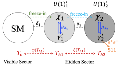
Figure 1: A graphic illustration of a general two-$U(1)$ model we discuss. The $U(1)_{1}^{\prime}$ hidden sector connects to the SM and the second hidden sector $U(1)_{2}^{\prime}$ via kinetic mixing characterized by parameters $\delta_{1}$ and $\delta_{2}$. Thus $U(1)_{2}^{\prime}$ couple to the SM indirectly and with the strength proportional to $\delta_{1}\times\delta_{2}$. $U(1)_{1}^{\prime}$ sector particles are produced via freeze-in processes from SM particles while $U(1)_{2}^{\prime}$ particles are produced via freeze-in mostly from the $U(1)_{1}^{\prime}$ sector. Each $U(1)$ hidden sector possesses a different temperature $T_{h1},T_{h2}$ respectively, related to the visible sector temperature $T_{v}$ through functions $\eta(T_{h1})=T_{v}/T_{h1}$ and $\zeta(T_{h1})=T_{h2}/T_{h1}$. The dark matter candidates are a combination of $\chi_{1},\chi_{2},\gamma_{2}^{\prime}$, among which $\gamma_{2}^{\prime}$ only occupies a tiny fraction of the total dark matter relic density and is responsible for the 511 keV signal through the decay $\gamma_{2}^{\prime}\to e^{+}e^{-}$.

The key idea of the model is simple: The tiny kinetic mixing $\delta_{1}\lesssim 10^{-10}$ can generate $U(1)_{1}^{\prime}$ sector particles via freeze-in mechanism, which can further produce $U(1)_{2}^{\prime}$ sector particles through freeze-in. The coupling between $U(1)_{2}^{\prime}$ and the SM is through the $U(1)_{1}^{\prime}$ sector and thus the coupling of $U(1)_{2}^{\prime}$ to the SM fermions is indirect and is proportional to $\delta_{1}\times\delta_{2}\lesssim 10^{-18}$, which can potentially explain the 511 keV signal. The dark photon $\gamma_{1}^{\prime}$ will decay to $e^{+}e^{-}$ before BBN. Dark matter candidates are generally a combination of $\chi_{1},\chi_{2},\gamma_{2}^{\prime}$, among which $\gamma_{2}^{\prime}$ with mass $2m_{e}\lesssim M_{\gamma_{2}^{\prime}}\lesssim 6\mathrm{MeV}$, only occupies a tiny fraction of the total dark matter relic density and is responsible for the 511 keV signal through the decay to $e^{+}e^{-}$ pairs. In certain parameter space one can easily arrange either $\chi_{1}$ or $\chi_{2}$ constitutes almost the full dark matter relic density, and thus the model shown in Fig. 1 can be simplified to two models shown in Fig. 3(a) and 3(b).

Now we rewrite the Lagrangian in the gauge eigenbasis $V^{T}=(D,C,B,A^{3})$, with the kinetic mixing matrix and mass mixing matrix given by

$$\mathcal{K}=\left(\begin{array}[]{cccc}1&\delta_{2}&0&0\\ \delta_{2}&1&\delta_{1}&0\\ 0&\delta_{1}&1&0\\ 0&0&0&1\end{array}\right)\,,\qquad M_{{\rm St}}^{2}=\left(\begin{array}[]{cccc}M_{2}^{2}\\ &M_{1}^{2}\\ &&\frac{1}{4}v^{2}g_{Y}^{2}&-\frac{1}{4}v^{2}g_{2}g_{Y}\\ &&-\frac{1}{4}v^{2}g_{2}g_{Y}&\frac{1}{4}v^{2}g_{2}^{2}\end{array}\right)\,,$$ (17)

which can be diagnolized simultaneously by the rotation matrix $\mathcal{R}$, transforming the gauge bosons in the gauge eigenbasis $(D,C,B,A^{3})^{T}$ into mass eigenbasis $(A^{\prime}_{2},A^{\prime}_{1},A^{\gamma},Z)^{T}$, representing the gauge fields of the two extra dark photons $\gamma^{\prime}_{2},\gamma^{\prime}_{1}$, the photon ($\gamma$) and $Z$ boson respectively. Details of derivation of the rotation matrix $\mathcal{R}$ using perturbation method, and the full expression of the matrix $\mathcal{R}$ are given in Appendix B.

With the mass eigenbasis, the neutral current couplings are calculated to be

$$\mathcal{L}_{ZA^{\prime}_{1}A^{\prime}_{2}A^{\gamma}}=\frac{1}{2}\bar{f_{i}}\gamma^{\mu}\left[\left(v_{i}-a_{i}\gamma^{5}\right)f_{i}Z_{\mu}+\left(v_{i}^{\prime}-a_{i}^{\prime}\gamma^{5}\right)f_{i}A_{1\mu}^{\prime}+\left(v_{i}^{\prime\prime}-a_{i}^{\prime\prime}\gamma^{5}\right)f_{i}A_{2\mu}^{\prime}\right]+eQ_{i}\bar{f_{i}}\gamma^{\mu}f_{i}A_{\mu}^{\gamma}\,,$$ (18)

where

$$v_{i}= \left(g_{2}\mathcal{R}_{44}-g_{Y}\mathcal{R}_{34}\right)T_{i}^{3}+2g_{Y}\mathcal{R}_{34}Q_{i}\,,\qquad a_{i}=\left(g_{2}\mathcal{R}_{44}-g_{Y}\mathcal{R}_{34}\right)T_{i}^{3}\,,$$ (19)

$$v_{i}^{\prime}= \left(g_{2}\mathcal{R}_{42}-g_{Y}\mathcal{R}_{32}\right)T_{i}^{3}+2g_{Y}\mathcal{R}_{32}Q_{i}\,,\qquad a_{i}^{\prime}=\left(g_{2}\mathcal{R}_{42}-g_{Y}\mathcal{R}_{32}\right)T_{i}^{3}\,,$$ (20)

$$v_{i}^{\prime\prime}= \left(g_{2}\mathcal{R}_{41}-g_{Y}\mathcal{R}_{31}\right)T_{i}^{3}+2g_{Y}\mathcal{R}_{31}Q_{i}\,,\qquad a_{i}^{\prime\prime}=\left(g_{2}\mathcal{R}_{41}-g_{Y}\mathcal{R}_{31}\right)T_{i}^{3}\,.$$ (21)

In the above equations, $eQ_{i},T_{i}$ are respectively the electric charge and the weak isospin of SM fermions. It’s straightforward to obtain the gauge bosons’ couplings with charged leptons and quarks

$$\mathcal{L}_{\gamma_{1}^{\prime}\bar{f_{i}}f_{i}}\approx\left(\delta_{1}g_{Y}c_{W}^{2}Q_{i}\right)\bar{f_{i}}\gamma^{\mu}f_{i}A_{1\mu}^{\prime}\,,\qquad\mathcal{L}_{\gamma_{2}^{\prime}\bar{f_{i}}f_{i}}\approx\left(\delta_{1}\delta_{2}g_{Y}c_{W}^{2}\beta^{2}Q_{i}\right)\bar{f_{i}}\gamma^{\mu}f_{i}A_{2\mu}^{\prime}\,,$$ (22)

where we have defined $\beta^{2}\equiv{M_{\gamma_{2}^{\prime}}^{2}}/{M_{\gamma_{1}^{\prime}}^{2}}$. The couplings of dark photons ($\gamma^{\prime}_{1},\gamma^{\prime}_{2}$) to SM neutrinos are however suppressed and can be safely neglected, which are given by

$$\mathcal{L}_{\gamma^{\prime}_{1}\bar{\nu}\nu} \approx-\frac{1}{2}\bigl{(}\delta_{1}\epsilon^{2}g_{Y}\bigr{)}\bar{\nu_{L}}\gamma^{\mu}\nu_{L}A_{1\mu}^{\prime}\,,$$ (23)

$$\mathcal{L}_{\gamma^{\prime}_{2}\bar{\nu}\nu} \approx\frac{-\delta_{1}\delta_{2}g_{Y}}{2N_{1}}\left[1+\epsilon^{2}(1+\beta^{2})-(1+\epsilon^{2})(1+\epsilon^{\prime 2})\right]\bar{\nu}_{L}\gamma^{\mu}\nu_{L}A_{2\mu}^{\prime}$$

$$\approx\frac{1}{2}\left(\delta_{1}\delta_{2}\epsilon^{2}\epsilon^{\prime 2}g_{Y}\right)\bar{\nu}_{L}\gamma^{\mu}\nu_{L}A_{2\mu}^{\prime}\,,$$ (24)

where

$$\epsilon\equiv\frac{M_{1}}{M_{Z}}\approx\frac{M_{\gamma^{\prime}_{1}}}{M_{Z}}\,,\qquad\epsilon^{\prime}\equiv\frac{M_{2}}{M_{Z}}\approx\frac{M_{\gamma^{\prime}_{2}}}{M_{Z}}\,.$$ (25)

Lastly, the interactions of ($Z,\gamma_{1}^{\prime},\gamma_{2}^{\prime}$) with dark fermions ($\chi_{1},\chi_{2}$) are given by

$$\mathcal{L}_{\chi_{1}} =g_{X_{1}}Q_{\chi_{1}}\left(\mathcal{R}_{24}Z_{\mu}+\mathcal{R}_{22}A_{1\mu}^{\prime}+\mathcal{R}_{21}A_{2\mu}^{\prime}\right)\bar{\chi}_{1}\gamma^{\mu}\chi_{1}\,,$$ (26)

$$\mathcal{L}_{\chi_{2}} =g_{X_{2}}Q_{\chi_{2}}\left(\mathcal{R}_{14}Z_{\mu}+\mathcal{R}_{12}A_{1\mu}^{\prime}+\mathcal{R}_{11}A_{2\mu}^{\prime}\right)\bar{\chi}_{2}\gamma^{\mu}\chi_{2}\,,$$ (27)

and thus

$$\mathcal{L}_{\gamma_{1}^{\prime}\bar{\chi}_{1}\chi_{1}} =g_{X_{1}}Q_{\chi_{1}}\bigl{(}\frac{1}{N_{2}}c_{1}c_{\psi}+\frac{\varepsilon_{12}}{N_{2}}c_{1}s_{2}\bigr{)}A_{1\mu}^{\prime}\bar{\chi}_{1}\gamma^{\mu}\chi_{1}$$

$$\approx g_{X_{1}}Q_{\chi_{1}}A_{1\mu}^{\prime}\bar{\chi}_{1}\gamma^{\mu}\chi_{1}\,,$$ (28)

$$\mathcal{L}_{\gamma_{2}^{\prime}\bar{\chi}_{1}\chi_{1}} =g_{X_{1}}Q_{\chi_{1}}\bigl{(}-\frac{c_{1}s_{2}}{N_{1}}+\frac{\varepsilon_{12}}{N_{1}}c_{1}c_{\psi}+\frac{\varepsilon_{14}}{N_{1}}c_{1}s_{\psi}\bigr{)}A_{2\mu}^{\prime}\bar{\chi}_{1}\gamma^{\mu}\chi_{1}$$

$$\approx g_{X_{1}}Q_{\chi_{1}}\delta_{2}\bigl{(}\frac{\beta^{2}}{1-\beta^{2}}+\delta_{1}^{2}s_{W}^{2}\bigr{)}A_{2\mu}^{\prime}\bar{\chi}_{1}\gamma^{\mu}\chi_{1}\,,$$ (29)

$$\mathcal{L}_{\gamma_{1}^{\prime}\bar{\chi}_{2}\chi_{2}} =g_{X_{2}}Q_{\chi_{2}}\bigl{(}-\frac{\varepsilon_{12}}{N_{2}}c_{2}\bigr{)}A_{1\mu}^{\prime}\bar{\chi}_{2}\gamma^{\mu}\chi_{2}\approx-g_{X_{2}}Q_{\chi_{2}}\bigl{(}\frac{\delta_{2}}{1-\beta^{2}}\bigr{)}A_{1\mu}^{\prime}\bar{\chi}_{2}\gamma^{\mu}\chi_{2}\,,$$ (30)

$$\mathcal{L}_{\gamma_{2}^{\prime}\bar{\chi}_{2}\chi_{2}} =g_{X_{2}}Q_{\chi_{2}}\bigl{(}\frac{c_{2}}{N_{1}}\bigr{)}A_{2\mu}^{\prime}\bar{\chi}_{2}\gamma^{\mu}\chi_{2}\approx g_{X_{2}}Q_{\chi_{2}}A_{2\mu}^{\prime}\bar{\chi}_{2}\gamma^{\mu}\chi_{2}\,.$$ (31)

3.2 Evolution of hidden sector particles in the two-$U(1)$ model

In this subsection we discuss full evolution of the two-$U(1)$ model shown in Fig. 1, using the method developed in [39, 40, 41, 64]. We assume negligible initial amount of particles in the two $U(1)$ sectors and $U(1)_{1}^{\prime}$ particles $\chi_{1},\gamma_{1}^{\prime}$ are produced through freeze-in processes from the SM particles: $i\bar{i}\to\chi_{1}\bar{\chi}_{1},\,i\bar{i}\to\gamma_{1}^{\prime}$; whereas the $U\left(1\right)_{2}^{\prime}$ particles $\chi_{2},\gamma_{2}^{\prime}$ are mostly produced from $U(1)_{1}^{\prime}$ sector: $\chi_{1}\bar{\chi}_{1}\to\chi_{2}\bar{\chi}_{2}$, $\chi_{1}\bar{\chi}_{1}\to\gamma_{1}^{\prime}\gamma_{2}^{\prime}$, $\gamma_{1}^{\prime}\gamma_{1}^{\prime}\to\chi_{2}\bar{\chi}_{2}$ and three-point process $\gamma_{1}^{\prime}\to\chi_{2}\bar{\chi}_{2}$ if $M_{\gamma_{1}^{\prime}}>2m_{\chi_{2}}$. The freeze-in processes to the $U(1)_{2}^{\prime}$ sector $\chi_{1}\bar{\chi}_{1}\to\gamma_{2}^{\prime}\gamma_{2}^{\prime}$, $i\bar{i}\to\chi_{2}\bar{\chi}_{2},\,i\bar{i}\to\gamma_{2}^{\prime}$ can be safely neglected in the computation. The inverse processes from the $U(1)_{2}^{\prime}$ sector $\chi_{2}\bar{\chi}_{2}\to\chi_{1}\bar{\chi}_{1}$, $\chi_{2}\bar{\chi}_{2}\to\gamma_{1}^{\prime}\gamma_{1}^{\prime}$, $\gamma_{1}^{\prime}\gamma_{2}^{\prime}\to\chi_{1}\bar{\chi}_{1}$ are also disregarded due to their negligible contributions.

The SM, $U(1)_{1}^{\prime}$, $U(1)_{2}^{\prime}$ sectors, possess different temperatures $T_{v},T_{h1},T_{h2}$ respectively and evolve almost independently, as a result of the tiny mixings between the three sectors. These three temperatures are related to each other with functions $\eta$($T_{h1}$)$\equiv T_{v}/T_{h1}$ and $\zeta$($T_{h1}$)$\equiv T_{h2}/T_{h1}$, and can be solved together with the evolution of the hidden sector particles. The dark particles among each $U(1)$ sector can have rather strong interactions including $\chi_{1}\bar{\chi}_{1}\leftrightarrow\gamma_{1}^{\prime}\gamma_{1}^{\prime}$, $\chi_{2}\bar{\chi}_{2}\leftrightarrow\gamma_{2}^{\prime}\gamma_{2}^{\prime}$, and $\chi_{1}\bar{\chi}_{1}\leftrightarrow\gamma_{1}^{\prime}$, which has significant impacts on the evolution of hidden sector particles. In the computation, we have taken into account all relevant interactions to calculate the complete evolution of all hidden sector particles.

The evolution of all hidden sector particles within the two-$U(1)$ model is governed by the coupled Boltzmann equations for comoving number densities $Y_{\chi_{1}},Y_{\gamma_{1}^{\prime}},Y_{\chi_{2}},Y_{\gamma_{2}^{\prime}}$ and the temperature functions $\eta(T_{h1}),\zeta(T_{h1})$:

$$\frac{\mathrm{d}Y_{\chi_{1}}}{\mathrm{d}T_{h1}}= -s\frac{\mathrm{d}\rho/\mathrm{d}T_{h1}}{4\rho H}\sum_{i\in\mathrm{SM}}\biggl{\{}\bigl{(}Y_{\chi_{1}}^{\mathrm{eq}}\bigr{)}^{2}\left\langle\sigma v\right\rangle_{\chi_{1}\bar{\chi}_{1}\to i\bar{i}}^{T_{h1}\eta}-Y_{\chi_{1}}^{2}\left\langle\sigma v\right\rangle_{\chi_{1}\bar{\chi}_{1}\to\chi_{2}\bar{\chi}_{2}}^{T_{h1}}$$

$$-Y_{\chi_{1}}^{2}\left\langle\sigma v\right\rangle_{\chi_{1}\bar{\chi}_{1}\to\gamma_{1}^{\prime}\gamma_{1}^{\prime}}^{T_{h1}}+Y_{\gamma_{1}^{\prime}}^{2}\left\langle\sigma v\right\rangle_{\gamma_{1}^{\prime}\gamma_{1}^{\prime}\to\chi_{1}\bar{\chi}_{1}}^{T_{h1}}-Y_{\chi_{1}}^{2}\left\langle\sigma v\right\rangle_{\chi_{1}\bar{\chi}_{1}\to\gamma_{1}^{\prime}\gamma_{2}^{\prime}}^{T_{h1}}$$

$$+\theta\bigl{(}M_{\gamma_{1}^{\prime}}-2m_{\chi_{1}}\bigr{)}\Bigl{[}-Y_{\chi_{1}}^{2}\left\langle\sigma v\right\rangle_{\chi_{1}\bar{\chi}_{1}\to\gamma_{1}^{\prime}}^{T_{h1}}+\frac{1}{s}Y_{\gamma_{1}^{\prime}}\bigl{\langle}\Gamma\bigr{\rangle}_{\gamma_{1}^{\prime}\to\chi_{1}\bar{\chi}_{1}}^{T_{h1}}\Bigr{]}\biggr{\}}\,,$$ (32)

$$\frac{\mathrm{d}Y_{\gamma_{1}^{\prime}}}{\mathrm{d}T_{h1}}= -s\frac{\mathrm{d}\rho/\mathrm{d}T_{h1}}{4\rho H}\sum_{i\in\mathrm{SM}}\biggl{\{}Y_{\chi_{1}}^{2}\left\langle\sigma v\right\rangle_{\chi_{1}\bar{\chi}_{1}\to\gamma_{1}^{\prime}\gamma_{1}^{\prime}}^{T_{h1}}-Y_{\gamma_{1}^{\prime}}^{2}\left\langle\sigma v\right\rangle_{\gamma_{1}^{\prime}\gamma_{1}^{\prime}\to\chi_{1}\bar{\chi}_{1}}^{T_{h1}}+Y_{\chi_{1}}^{2}\left\langle\sigma v\right\rangle_{\chi_{1}\bar{\chi}_{1}\to\gamma_{1}^{\prime}\gamma_{2}^{\prime}}^{T_{h1}}$$

$$-Y_{\gamma_{1}^{\prime}}^{2}\left\langle\sigma v\right\rangle_{\gamma_{1}^{\prime}\gamma_{1}^{\prime}\to\chi_{2}\bar{\chi}_{2}}^{T_{h1}}+\theta\bigl{(}M_{\gamma_{1}^{\prime}}-2m_{i}\bigr{)}\Bigl{[}Y_{i}^{2}\left\langle\sigma v\right\rangle_{i\bar{i}\to\gamma_{1}^{\prime}}^{T_{h1}\eta}-\frac{1}{s}Y_{\gamma_{1}^{\prime}}\bigl{\langle}\Gamma\bigr{\rangle}_{\gamma_{1}^{\prime}\to i\bar{i}}^{T_{h1}}\Bigr{]}$$

$$+\theta\bigl{(}M_{\gamma_{1}^{\prime}}-2m_{\chi_{1}}\bigr{)}\Bigl{[}Y_{\chi_{1}}^{2}\left\langle\sigma v\right\rangle_{\chi_{1}\bar{\chi}_{1}\to\gamma_{1}^{\prime}}^{T_{h1}}-\frac{1}{s}Y_{\gamma_{1}^{\prime}}\bigl{\langle}\Gamma\bigr{\rangle}_{\gamma_{1}^{\prime}\to\chi_{1}\bar{\chi}_{1}}^{T_{h1}}\Bigr{]}$$

$$+\theta\bigl{(}M_{\gamma_{1}^{\prime}}-2m_{\chi_{2}}\bigr{)}\Bigl{[}Y_{\chi_{2}}^{2}\left\langle\sigma v\right\rangle_{\chi_{2}\bar{\chi}_{2}\to\gamma_{1}^{\prime}}^{T_{h1}\zeta}-\frac{1}{s}Y_{\gamma_{1}^{\prime}}\bigl{\langle}\Gamma\bigr{\rangle}_{\gamma_{1}^{\prime}\to\chi_{2}\bar{\chi}_{2}}^{T_{h1}}\Bigr{]}\biggr{\}}\,,$$ (33)

$$\frac{\mathrm{d}Y_{\chi_{2}}}{\mathrm{d}T_{h1}}= -s\frac{\mathrm{d}\rho/\mathrm{d}T_{h1}}{4\rho H}\sum_{i\in\mathrm{SM}}\biggl{\{}Y_{\gamma_{1}^{\prime}}^{2}\left\langle\sigma v\right\rangle_{\gamma_{1}^{\prime}\gamma_{1}^{\prime}\to\chi_{2}\bar{\chi}_{2}}^{T_{h1}}+Y_{\chi_{1}}^{2}\left\langle\sigma v\right\rangle_{\chi_{1}\bar{\chi}_{1}\to\chi_{2}\bar{\chi}_{2}}^{T_{h1}}-Y_{\chi_{2}}^{2}\left\langle\sigma v\right\rangle_{\chi_{2}\bar{\chi}_{2}\to\gamma_{2}^{\prime}\gamma_{2}^{\prime}}^{T_{h1}\zeta}$$

$$+Y_{\gamma_{2}^{\prime}}^{2}\left\langle\sigma v\right\rangle_{\gamma_{2}^{\prime}\gamma_{2}^{\prime}\to\chi_{2}\bar{\chi}_{2}}^{T_{h1}\zeta}+\theta\bigl{(}M_{\gamma_{1}^{\prime}}-2m_{\chi_{2}}\bigr{)}\Bigl{[}-Y_{\chi_{2}}^{2}\left\langle\sigma v\right\rangle_{\chi_{2}\bar{\chi}_{2}\to\gamma_{1}^{\prime}}^{T_{h1}\zeta}+\frac{1}{s}Y_{\gamma_{1}^{\prime}}\bigl{\langle}\Gamma\bigr{\rangle}_{\gamma_{1}^{\prime}\to\chi_{2}\bar{\chi}_{2}}^{T_{h1}}\Bigr{]}\biggr{\}}\,,$$ (34)

$$\frac{\mathrm{d}Y_{\gamma_{2}^{\prime}}}{\mathrm{d}T_{h1}}= -s\frac{\mathrm{d}\rho/\mathrm{d}T_{h1}}{4\rho H}\sum_{i\in\mathrm{SM}}\Bigl{[}Y_{\chi_{1}}^{2}\left\langle\sigma v\right\rangle_{\chi_{1}\bar{\chi}_{1}\to\gamma_{1}^{\prime}\gamma_{2}^{\prime}}^{T_{h1}}+Y_{\chi_{2}}^{2}\left\langle\sigma v\right\rangle_{\chi_{2}\bar{\chi}_{2}\to\gamma_{2}^{\prime}\gamma_{2}^{\prime}}^{T_{h1}\zeta}-Y_{\gamma_{2}^{\prime}}^{2}\left\langle\sigma v\right\rangle_{\gamma_{2}^{\prime}\gamma_{2}^{\prime}\to\chi_{2}\bar{\chi}_{2}}^{T_{h1}\zeta}\Bigr{]}\,,$$ (35)

$$\frac{\mathrm{d}\eta}{\mathrm{d}T_{h1}}= -\frac{\eta}{T_{h1}}+\frac{1}{T_{h1}}\left(\frac{4H\rho_{v}+j_{h1}+j_{h2}}{4H\rho_{h1}-j_{h1}}\right)\frac{\mathrm{d}\rho_{h1}/\mathrm{d}T_{h1}}{\mathrm{d}\rho_{v}/\mathrm{d}T_{v}}\,,$$ (36)

$$\frac{\mathrm{d}\zeta}{\mathrm{d}T_{h1}}= -\frac{\zeta}{T_{h1}}+\frac{1}{T_{h1}}\left(\frac{4H\rho_{h2}-j_{h2}}{4H\rho_{h1}-j_{h1}}\right)\frac{\mathrm{d}\rho_{h1}/\mathrm{d}T_{h1}}{\mathrm{d}\rho_{h2}/\mathrm{d}T_{h2}}\,,$$ (37)

where the energy transfer densities of two hidden sectors are given by

$$j_{h1}= \sum_{i\in\mathrm{SM}}\Bigl{[}2Y_{i}^{2}s^{2}J_{i\bar{i}\to\chi_{1}\bar{\chi}_{1}}^{T_{h1}\eta}-2Y_{\chi_{1}}^{2}s^{2}J_{\chi_{1}\bar{\chi}_{1}\to\chi_{2}\bar{\chi}_{2}}^{T_{h1}}-Y_{\chi_{1}}^{2}s^{2}J_{\chi_{1}\bar{\chi}_{1}\to\gamma_{1}^{\prime}\gamma_{2}^{\prime}}^{T_{h1}}$$

$$-2Y_{\gamma_{1}^{\prime}}^{2}s^{2}J_{\gamma_{1}^{\prime}\gamma_{1}^{\prime}\to\chi_{2}\bar{\chi}_{2}}^{T_{h1}}+\theta\bigl{(}M_{\gamma_{1}^{\prime}}-2m_{i}\bigr{)}\Bigl{(}Y_{i}^{2}s^{2}J_{i\bar{i}\to\gamma_{1}^{\prime}}^{T_{h1}\eta}-Y_{\gamma_{1}^{\prime}}sJ_{\gamma_{1}^{\prime}\to i\bar{i}}^{T_{h1}}\Bigr{)}$$

$$+\theta\bigl{(}M_{\gamma_{1}^{\prime}}-2m_{\chi_{2}}\bigr{)}\Bigl{(}Y_{\chi_{2}}^{2}s^{2}J_{\chi_{2}\bar{\chi}_{2}\to\gamma_{1}^{\prime}}^{T_{h1}\zeta}-Y_{\gamma_{1}^{\prime}}sJ_{\gamma_{1}^{\prime}\to\chi_{2}\bar{\chi}_{2}}^{T_{h1}}\Bigr{)}\Bigr{]}\,,$$ (38)

$$j_{h2}= \sum_{i\in\mathrm{SM}}\Bigl{[}2Y_{\chi_{1}}^{2}s^{2}J_{\chi_{1}\bar{\chi}_{1}\to\chi_{2}\bar{\chi}_{2}}^{T_{h1}}+Y_{\chi_{1}}^{2}s^{2}J_{\chi_{1}\bar{\chi}_{1}\to\gamma_{1}^{\prime}\gamma_{2}^{\prime}}^{T_{h1}}+2Y_{\gamma_{1}^{\prime}}^{2}s^{2}J_{\gamma_{1}^{\prime}\gamma_{1}^{\prime}\to\chi_{2}\bar{\chi}_{2}}^{T_{h1}}$$

$$+\theta\bigl{(}M_{\gamma_{1}^{\prime}}-2m_{\chi_{2}}\bigr{)}\Bigl{(}-2Y_{\chi_{2}}^{2}s^{2}J_{\chi_{2}\bar{\chi}_{2}\to\gamma_{1}^{\prime}}^{T_{h1}\zeta}+2Y_{\gamma_{1}^{\prime}}sJ_{\gamma_{1}^{\prime}\to\chi_{2}\bar{\chi}_{2}}^{T_{h1}}\Bigr{)}\Bigr{]}\,.$$ (39)

We explore two cases to explain the 511 keV flux, each possessing three components of the dark matter candidates $\{\chi_{1},\chi_{2},\gamma_{2}^{\prime}\}$ offered by both two $U(1)$ sectors with different proportion in the total dark matter relic density. For each case, we consider three different benchmark models depending on the masses of $\gamma^{\prime}_{1}$ and $\chi_{1}$: $M_{\gamma^{\prime}_{1}}<m_{\chi_{1}}$, $m_{\chi_{1}}<M_{\gamma^{\prime}_{1}}<2m_{\chi_{1}}$, and $M_{\gamma^{\prime}_{1}}>2m_{\chi_{1}}$.

Case

1: $M_{\gamma^{\prime}_{1}}<2m_{\chi_{2}}$ (the dark matter is predominantly $\chi_{1}$) In this case, the $U(1)^{\prime}_{2}$ sector particles $\chi_{2},\gamma^{\prime}_{2}$ are produced via freeze-in from the $U(1)^{\prime}_{1}$ sector through four-point interactions $\gamma_{1}^{\prime}\gamma_{1}^{\prime}\to\chi_{2}\bar{\chi}_{2}$, $\chi_{1}\bar{\chi}_{1}\to\chi_{2}\bar{\chi}_{2}$, $\chi_{1}\bar{\chi}_{1}\to\gamma_{1}^{\prime}\gamma_{2}^{\prime}$. Particles within each hidden sector can have vigorous interactions including $\chi_{1}\bar{\chi}_{1}\leftrightarrow\gamma_{1}^{\prime}$ or $\chi_{1}\bar{\chi}_{1}\leftrightarrow\gamma_{1}^{\prime}\gamma_{1}^{\prime}$, $\chi_{2}\bar{\chi}_{2}\leftrightarrow\gamma_{2}^{\prime}\gamma_{2}^{\prime}$. As the temperature drops down, the $U(1)^{\prime}_{1}$ hidden sector will encounter the freeze-out of $\chi_{1}$ or $\gamma^{\prime}_{1}$ depending on their masses. Eventually all of the dark photon $\gamma_{1}^{\prime}$ will decay into SM fermions through $\gamma_{1}^{\prime}\to i\bar{i}$ before BBN, and the remaining $\chi_{1}$ constitutes the dominant dark matter candidate. The dark particles $\chi_{2},\gamma_{2}^{\prime}$ occupy only a tiny fraction of the total dark matter relic density. The 511 keV signal is interpreted by the decay $\gamma_{2}^{\prime}\to e^{+}e^{-}$.

Case

2: $M_{\gamma_{1}^{\prime}}>2m_{\chi_{2}}$ (the dark matter is predominantly $\chi_{2}$) In this case, the dark fermion $\chi_{2}$ is mainly produced by the intensive decay process $\gamma^{\prime}_{1}\to\chi_{2}\bar{\chi}_{2}$, and can interact with the dark photon $\gamma_{2}^{\prime}$ through $\chi_{2}\bar{\chi}_{2}\leftrightarrow\gamma_{2}^{\prime}\gamma_{2}^{\prime}$, producing the desired amount of the dark photon $\gamma^{\prime}_{2}$ to explain the 511 keV signal. The $U(1)^{\prime}_{1}$ gauge boson $\gamma_{1}^{\prime}$ can also interchange with $\chi_{1}$ or decay into SM fermions and finally reach a negligible amount. The dark matter can primarily consist of $\chi_{2}$, with minor contribution from $\chi_{1}$ and $\gamma^{\prime}_{2}$. The 511 keV signal is also attributed to the dark photon $\gamma^{\prime}_{2}$ via its decay into $e^{+}e^{-}$.

The model shown in Fig. 1 is robust. In addition to Case 1 and Case 2, we can also adjust the parameter values such that both $\chi_{1}$ and $\chi_{2}$ constitute significant fractions of the total dark matter relic density.

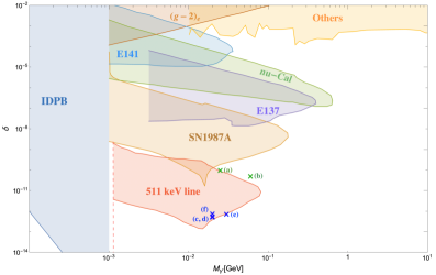
Figure 2: [color online] A display of current experimental constraints (colored regions) on the kinetic mixing parameter. We also include the constraint from 511 keV signal discussed in Section 2.2.3 (the region in red) [59]. This constraint is only valid for a dark photon that can decay only into $e^{+}e^{-}$. Benchmark models a and b fall into this category, thus we choose parameters outside this red region. In benchmark models c-f, the dark photon can also decay into dark matter, allowing this constraint to be circumvented. Hence, we can safely choose parameter values within the red region.

As discussed in Section 2.2.3, $\mathcal{O}$(MeV) scale particles interacting feebly with SM fields can be produced in a supernova core and decay into electron-positron pairs outside the supernova envelope, subject to stringent constraints from the observed 511 keV photon emission. The energy loss of SN 1987A as well as various laboratory experiments also impose limits on the model parameters. In the literature, constraints on the kinetic mixing parameter $\bm{\delta}$ is usually obtained from a simplified model that the dark photon mixed directly with the photon field. A more precise treatment is to consider the dark photon mixed with the hypercharge [65, 42], where the kinetic mixing parameter is denoted by $\delta$, as was discussed in this paper. We translate the experimental constraints on $\bm{\delta}$ to $\delta$ using the relation [42]

$$\delta_{1}=\frac{\sqrt{g_{2}^{2}+g_{Y}^{2}}}{g_{2}}\bm{\delta}\,.$$ (40)

The current experimental constraints on the kinetic mixing parameter $\delta_{1}$ in terms of the dark photon mass is plotted in Fig. 2 with all our benchmark models marked respectively.

Case	Model	$m_{\chi_{1}}$	$m_{\chi_{2}}$	$M_{\gamma_{1}^{\prime}}$	$\delta_{1}$	$\delta_{2}$	$g_{X_{1}}$	$g_{X_{2}}$	$\Omega_{\chi_{1}}h^{2}$	$\Omega_{\chi_{2}}h^{2}$	$\Omega_{\gamma_{2}^{\prime}}h^{2}$	$\tau_{\gamma_{1}^{\prime}}$	$\tau_{\gamma_{2}^{\prime}}$
$M_{\gamma_{1}^{\prime}}<2m_{\chi_{2}}$	$a$	$35$	$30$	$25$	$1\times 10^{-10}$	$9.5\times 10^{-9}$	$6.15\times 10^{-3}$	$0.08$	$0.12$	$1.1\times 10^{-7}$	$6.5\times 10^{-9}$	$0.49$	$1.6\times 10^{19}$
	$b$	$40$	$35$	$60$	$5.2\times 10^{-11}$	$4.5\times 10^{-7}$	$3.8\times 10^{-5}$	$0.92$	$0.12$	$2.5\times 10^{-10}$	$6.8\times 10^{-10}$	$0.76$	$9.8\times 10^{17}$
	$c$	$8$	$25$	$20$	$5.8\times 10^{-13}$	$5\times 10^{-6}$	$7\times 10^{-3}$	$0.5$	$0.12$	$2.1\times 10^{-12}$	$2.8\times 10^{-10}$	$3.2\times 10^{-17}$	$6.6\times 10^{17}$
$M_{\gamma_{1}^{\prime}}>2m_{\chi_{2}}$	$d$	$30$	$9$	$20$	$5.3\times 10^{-13}$	$3\times 10^{-6}$	$1\times 10^{-5}$	$2.5\times 10^{-5}$	$1.7\times 10^{-13}$	$0.12$	$9.4\times 10^{-10}$	$0.83$	$2.2\times 10^{18}$
	$e$	$20$	$14$	$30$	$7.6\times 10^{-13}$	$4\times 10^{-6}$	$1\times 10^{-5}$	$3.7\times 10^{-5}$	$5.0\times 10^{-11}$	$0.12$	$2.0\times 10^{-9}$	$0.21$	$3.4\times 10^{18}$
	$f$	$8$	$9$	$20$	$7.8\times 10^{-13}$	$4.5\times 10^{-6}$	$1\times 10^{-12}$	$2\times 10^{-5}$	$1.3\times 10^{-5}$	$0.12$	$3.8\times 10^{-10}$	$0.21$	$4.9\times 10^{17}$

Table 1: The benchmark models we consider in this work for Case 1 and Case 2. In both cases, $M_{\gamma_{2}^{\prime}}$ is taken to be 6 MeV to explain the 511 keV signal. The lifetimes of the two dark photons (in the unit of seconds) for each model are listed in the last two columns, ensuring $\gamma^{\prime}_{1}$ decays before BBN while the lifetime of $\gamma^{\prime}_{2}$ exceeds the age of the Universe. All benchmark models satisfy all relevant experimental constraints and are also marked in Fig. 2. All masses are in the unit of MeVs. In both of Case 1 and Case 2, there is plenty of parameter space available for adjustment, such that both $\chi_{1}$ and $\chi_{2}$ constitute significant fractions of the total dark matter relic density.

The benchmark models we consider are listed in Table 1. In all these models, the 511 keV signal is emitted by the process $\gamma_{2}^{\prime}\to e^{+}e^{-}$, where the $U(1)_{2}^{\prime}$ gauge boson $\gamma_{2}^{\prime}$ with mass $2m_{e}\lesssim M_{\gamma_{2}^{\prime}}\lesssim 6\mathrm{MeV}$ and lifetime exceeding the age of the Universe, constitutes only a small fraction of the total dark matter relic density. The $U(1)^{\prime}_{1}$ sector gauge boson $\gamma_{1}^{\prime}$ will decay before BBN.

As shown in Fig. 2, in addition to the SN 1987A bound on the extra $U(1)$, the 511 keV signal provide more stringent constraints on the dark photon mixing [59], which is the most sensitive region for our analysis. The 511 keV signal constraint is only valid for models that the dark photon can decay only into $e^{+}e^{-}$, In models a and b, marked by the shaded light green in Table 1, the dark photon $\gamma^{\prime}_{1}$ will decay to $e^{+}e^{-}$, thus suffered from the constraints. We choose the parameter values outside the red region in Fig. 2 for models a and b. For models c-f, marked by the shaded light blue in Table 1, the dark photon $\gamma^{\prime}_{1}$ will mostly decay into dark fermion pairs and the 511 keV signal constraint does not impose constraints on these models. We can then choose the parameters within the red region in Fig. 2 safely for models c-f.

In the computation of solving the coupled Boltzmann equations Eqs.(32)-(39), we take the initial values of $\eta=10,\,\zeta=0.1$ at the temperature $T_{h1}=10^{5}$ GeV. We take the benchmark models a and d as examples to illustrate the details of the hidden sector evolution. The full evolution of hidden sector particles as well as the interaction rates of several important processes among $U(1)$ hidden sectors compared with the Hubble parameter versus temperature are plotted in Fig. 3 Panels (c) and (d).

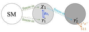
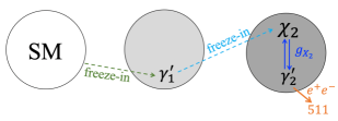
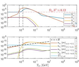
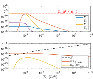
Figure 3: [Color online] An exhibition of the evolution for the two $U(1)$ hidden sectors, for Case 1 (using model a as an illustration) and Case 2 (using model d as an illustration). In Case 1, we arrange the parameters in such a way that $\chi_{1}$ is the main component of dark matter; whereas in Case 2, $\chi_{2}$ is the main component of dark matter. Thus the two-$U(1)$ model can be reduced to Panel (a) for Case 1 and Panel (b) for Case 2. Panels (c) and (d) show the evolution of the hidden sector particles as well as the interaction rates of hidden sector interactions compared with the Hubble parameter, for model a and model d respectively. In Panels (c) and (d), the above figure shows the evolution of the comoving number densities of all dark particles in two $U(1)$ hidden sectors. The red horizontal line denoting the observed dark matter relic density. In the lower figures, interaction rates for various interactions among the hidden sectors as well as the Hubble parameter versus temperature are presented.

As we can see from Fig. 3 Panel (c), for Case 1 model a, the comoving number densities of the $U(1)^{\prime}_{1}$ sector particles $\chi_{1},\gamma^{\prime}_{1}$ accumulate via the freeze-in processes $i\bar{i}\to\chi_{1}\bar{\chi}_{1}$, $i\bar{i}\to\gamma^{\prime}_{1}$, and later reach the thermal equilibrium within the $U(1)^{\prime}_{1}$ sector. The black vertical dash line marks the temperature at which the interaction rate of the process $\gamma_{1}^{\prime}\gamma_{1}^{\prime}\to\chi_{1}\bar{\chi}_{1}$ drops below the Hubble line, which indicate the process $\gamma_{1}^{\prime}\gamma_{1}^{\prime}\to\chi_{1}\bar{\chi}_{1}$ becomes inactive and thus the dark freeze-out occurs in the $U(1)_{1}^{\prime}$ sector, corresponding to the number density of $\chi_{1}$ going down. The dark freeze-out ended as the process $\chi_{1}\bar{\chi}_{1}\to\gamma_{1}^{\prime}\gamma_{1}^{\prime}$ becoming inactive, denoted by the black vertical dash-dotted line, and the number density of $\chi_{1}$ tends to level off at the observed value of dark matter relic density. The light blue line in the lower figure shows the thermally averaged decay width of $\gamma_{1}^{\prime}$ to SM fermion pairs starts to exceed the Hubble line and since then $\gamma_{1}^{\prime}$ will decay out of equilibrium, and the number density of $\gamma_{1}^{\prime}$ eventually decline to zero before BBN. The dark fermion $\chi_{2}$ and the dark photon $\gamma_{2}^{\prime}$ are primarily produced by the $U(1)_{1}^{\prime}$ sector particles through the interactions $\chi_{1}\bar{\chi}_{1}\to\chi_{2}\bar{\chi}_{2}$, $\chi_{1}\bar{\chi}_{1}\to\gamma_{1}^{\prime}\gamma_{2}^{\prime}$, $\gamma_{1}^{\prime}\gamma_{1}^{\prime}\to\chi_{2}\bar{\chi}_{2}$, while the freeze-in from SM particles such as $i\bar{i}\to\chi_{2}\bar{\chi}_{2}$, $i\bar{i}\to\gamma_{2}^{\prime}$ can be safely ignored. Within the $U(1)_{2}^{\prime}$ sector, interactions $\chi_{2}\bar{\chi}_{2}\leftrightarrow\gamma_{2}^{\prime}\gamma_{2}^{\prime}$ have important impacts on the final relic abundance of $\chi_{2},\gamma_{2}^{\prime}$ related to $g_{X_{2}}$.

For Case 2 model d shown in Fig. 3 Panel (d), the couplings are set with the relation $\delta_{1}\ll g_{X_{2}}\delta_{2}$, resulting in most of $\gamma^{\prime}_{1}$ decaying into the dark fermion $\chi_{2}$ through the intensive process $\gamma^{\prime}_{1}\to\chi_{2}\bar{\chi}_{2}$, and thus circumvent the 511 keV signal constraints shown in Fig. 2. In Fig. 3 Panel (d), the black vertical dash line shows the temperature at which the thermally averaged decay width of $\gamma^{\prime}_{1}\to\chi_{2}\bar{\chi}_{2}$ exceeds the Hubble line and thus this decay process becomes active, in accordance with a steep drop of the number density of $\gamma^{\prime}_{1}$. The production of dark photon $\gamma^{\prime}_{2}$ is dominated by the interaction $\chi_{2}\bar{\chi}_{2}\to\gamma_{2}^{\prime}\gamma_{2}^{\prime}$ within the $U(1)^{\prime}_{2}$ hidden sector. The dark photon $\gamma^{\prime}_{2}$ ultimately constitutes a small fraction of the total dark matter content, contributing to the 511 keV flux through decay $\gamma^{\prime}_{2}\to e^{+}e^{-}$.

3.3 Interpretation of the 511 keV signal from $\gamma^{\prime}_{2}$ decay

For all benchmark models we investigate in this work, shown in Table 1, the dark photon $\gamma_{2}^{\prime}$, which constitutes a minor fraction of the total observed dark matter relic density, can decay primarily into $e^{+}e^{-}$ pairs, offering a potential explanation for the observed galactic 511 keV signal. Using Eqs. (7)-(9), the 511 keV photon flux generated by the decay of the dark photon $\gamma^{\prime}_{2}$ is computed to be

$$\Phi_{511}=\frac{f_{\gamma^{\prime}_{2}}}{8\pi}\int\mathrm{d}\Omega\int_{\mathrm{l.o.s}}\frac{\rho\left(r\right)}{M_{\gamma_{2}^{\prime}}}\Gamma_{\gamma^{\prime}_{2}\to e^{+}e^{-}}\mathrm{d}s\,,$$ (41)

where the decay width $\Gamma_{\gamma^{\prime}_{2}\to e^{+}e^{-}}$ is given by

$$\Gamma_{\gamma_{2}^{\prime}\to e^{+}e^{-}} \approx\frac{(\delta_{1}\delta_{2}g_{Y}c_{W}^{2}\beta^{2})^{2}}{12\pi}M_{\gamma_{2}^{\prime}}\sqrt{1-\frac{4m_{e}^{2}}{M_{\gamma_{2}^{\prime}}^{2}}}\biggl{(}1+\frac{2m_{e}^{2}}{M_{\gamma_{2}^{\prime}}^{2}}\biggr{)}\>,$$ (42)

with $\beta^{2}\equiv M_{\gamma_{2}^{\prime}}^{2}/M_{\gamma_{1}^{\prime}}^{2}$ defined earlier.

We adopt a NFW profile and an Einasto profile, c.f., Eqs. (10)-(11), with $\gamma=1$, $\alpha=0.17$, $r_{s}=20\leavevmode\nobreak\ \mathrm{kpc}$, and the scale density $\rho_{s}$ is normalized by the local density $\rho_{\odot}=0.43\leavevmode\nobreak\ \mathrm{\,GeV/cm^{3}}$ [66] at the Sun’s location $R_{\odot}=8.5\leavevmode\nobreak\ \mathrm{kpc}$. The bulge flux can be calculated by integrating over the inner part of the Galaxy ($|l|\lesssim 30^{\circ}$, $|b|\lesssim 15^{\circ}$), or over the Gaussian full-width-half-maximum (FWHM) corresponding to half of the total value. In Table 2 we list the results of bulge flux for benchmark model a including two integration range under the NFW and Einasto profile, which are consistent with the measured bulge flux [11]. The bulge flux for other benchmark models can also be obtained in the same way.

The bulge flux	$\Phi_{511}^{\mathrm{NFW}}$	$\Phi_{511}^{\mathrm{Einasto}}$
$|l|\lesssim 30^{\circ}$, $|b|\lesssim 15^{\circ}$	8.3	9.7
FWHM $\simeq 20.55^{\circ}$	4.8	6.0

Table 2: The results of bulge flux for benchmark model a using different integral range for the two dark matter density profile we consider. All fluxes are in units of $10^{-4}\leavevmode\nobreak\ \mathrm{\,ph\,cm^{-2}\,s^{-1}}$ and the FWHM value used here is for the broad bulge.

Finally we summarize the following relation

$$\frac{\tau_{X\to e^{+}e^{-}}(\mathrm{sec})\times M_{X}(\mathrm{MeV})}{f_{X}\times\mathrm{Br}(X\to e^{+}e^{-})}\sim 10^{27}\,,$$ (43)

for the parameter values we take in the dark matter profiles, to explain the 511 keV photon signal by the dark matter $X$ decaying to $e^{+}e^{-}$ pairs. We find the two-$U(1)$ model discussed in this paper remains highly promising in addressing the 511 keV signal consistent with various dark matter density profiles.

4 Conclusion

In recent years, various dark matter direct and indirect detections experiments, from earth-based experiments to astrophysical measurements, impose stringent bounds to dark matter models. Thus the parameter space for a large number of dark matter models are severely constrained. The relic density $\Omega h^{2}=0.12$ now becomes a constraint to the dark matter model rather than a ultimate goal to achieve.

The galactic 511 keV photon signal has been a longstanding discoveries for over half a century, but without a widely accepted explanation. In this paper we explore the decaying dark matter interpretation of the 511 keV signal. We consider a two-step freeze-in procedure which generates a dark photon dark matter with lifetime exceeding the age of the Universe, but can decay to $e^{+}e^{-}$ in tiny amount and potentially explain the 511 keV photon emission.

We discuss in general the kinetic mixing between two extra $U(1)$ gauge fields and the hypercharge gauge field. We derive the diagonalization of the mixing matrix by using the perturbation method and carry out all relevant couplings between hidden sector particles and SM particles. We compute the full evolution of the two extra $U(1)$ sector beyond the SM and discuss several characteristic benchmark models in two different cases. In the two-$U(1)$ model, the dark photon dark matter can be fully responsible for the 511 keV signal. The freeze-in mechanism can generate the entire dark matter relic abundance in the model, other sources for any types of additional dark matter components are unnecessary.

We extensively investigate the decaying dark matter interpretation of the 511 keV photon signal and find the two-$U(1)$ model discussed in this work remains a strong candidate for explaining the 511 keV signal in concordance with various dark matter density profiles.

Acknowledgments:

WZF has benefited from useful discussions with Xiaoyong Chu. This work is supported by the National Natural Science Foundation of China under Grant No. 11935009.

Appendix A Multi-temperature universe and evolution of hidden sector particles

In this Appendix we review the derivation of the evolution of hidden sector particles and the hidden sector temperature [39], for the one hidden sector extension of the SM. Assuming the hidden sector interacts with the visible sector feebly and hidden sector possess a separate temperature $T_{h}$ compared to the visible sector temperature $T$ (the temperature of the observed universe). From Friedmann equations we have

$$\frac{{\rm d}\rho_{h}}{{\rm d}t}+3H\left(\rho_{h}+p_{h}\right)=j_{h}\,,$$ (44)

where $\rho_{h}(p_{h})$ is the hidden sector energy density (pressure) determined by the particles inside the hidden sector, e.g., in the single-$U(1)$ extension of the SM, one has $\rho_{h}=\rho_{\gamma^{\prime}}+\rho_{\chi}$ and $p_{h}=p_{\gamma^{\prime}}+p_{\chi}$.

The total energy density in the universe $\rho$ is a sum of $\rho_{h}$ and $\rho_{v}$ (the energy density in the visible sector), giving rise to the Hubble parameter depending on both $T$ and $T_{h}$

$$H^{2}=\frac{8\pi G_{N}}{3}\big{[}\rho_{v}(T)+\rho_{h}(T_{h})\big{]}=\frac{8\pi G_{N}}{3}\left(\frac{\pi^{2}}{30}g_{{\rm eff}}^{v}T^{4}+\frac{\pi^{2}}{30}g_{{\rm eff}}^{h}T_{h}^{4}\right)\,,$$ (45)

where $g_{{\rm eff}}^{v}\,(g_{{\rm eff}}^{h})$ is the visible (hidden) effective degrees of freedom. Further one can deduct the derivative of $\rho_{v},\rho_{h}$ w.r.t. $T_{h}$

$$\rho\frac{{\rm d}\rho_{h}}{{\rm d}T_{h}} =\left(\frac{\zeta_{h}}{\zeta}\rho_{h}-\frac{j_{h}}{4H\zeta}\right)\frac{{\rm d}\rho}{{\rm d}T_{h}}\,,$$ (46)

$$\frac{{\rm d}\rho_{v}}{{\rm d}T_{h}} =\frac{\zeta\rho_{v}+\rho_{h}(\zeta-\zeta_{h})+j_{h}/(4H)}{\zeta_{h}\rho_{h}-j_{h}/(4H)}\frac{{\rm d}\rho_{h}}{{\rm d}T_{h}}\,,$$ (47)

where $\zeta=\frac{3}{4}(1+p/\rho)$. Here $\zeta=1$ is for the radiation dominated era and $\zeta=3/4$ for the matter dominated universe. The total entropy of the universe is conserved and thus

$$s =\frac{2\pi^{2}}{45}\big{(}h_{{\rm eff}}^{v}T^{3}+h_{{\rm eff}}^{h}T_{h}^{3}\big{)}\,,$$ (48)

where $h_{{\rm eff}}^{v}\,(h_{{\rm eff}}^{h})$ is the visible (hidden) effective entropy degrees of freedom.

With manipulations of the above equations, the evolution of the ratio of temperatures for the two sectors $\eta(T_{h})=T/T_{h}$ can be derived as

$$\frac{{\rm d}\eta}{{\rm d}T_{h}}=-\frac{A_{v}}{B_{v}}+\frac{\zeta\rho_{v}+\rho_{h}(\zeta-\zeta_{h})+j_{h}/(4H)}{B_{v}[\zeta_{h}\rho_{h}-j_{h}/(4H)]}\frac{{\rm d}\rho_{h}}{{\rm d}T_{h}}\,,$$ (49)

with

$$A_{v}=\frac{\pi^{2}}{30}\Big{(}\frac{{\rm d}g_{{\rm eff}}^{v}}{{\rm d}T}\eta^{5}T_{h}^{4}+4g_{{\rm eff}}^{v}\eta^{4}T_{h}^{3}\Big{)}\,,\qquad B_{v}=\frac{\pi^{2}}{30}\Big{(}\frac{{\rm d}g_{{\rm eff}}^{v}}{{\rm d}T}\eta^{4}T_{h}^{5}+4g_{{\rm eff}}^{v}\eta^{3}T_{h}^{4}\Big{)}\,.$$ (50)

The complete evolution of hidden sector particles can be obtained by solving the combined differential equations of the evolution equation for $\eta(T_{h})$, together with the modified (temperature dependent) Boltzmann equations for the hidden sector particles, given by

$$\frac{\mathrm{d}Y_{i}}{\mathrm{d}T_{h}}=-\frac{s}{H}\frac{{\rm d}\rho_{h}/{\rm d}T_{h}}{4\rho_{h}-j_{h}/H}\sum\big{(}-Y_{i}^{2}\langle\sigma v\rangle^{T_{h}}_{i\bar{i}\to\times\times}+\cdots\big{)}\,,$$ (51)

where $Y_{i}$ is the comoving number density of the $i$th hidden sector particle and the sum is over various scatter or decay processes involving this particle, which may depend on $T_{h}$ (as shown by the example ${i\bar{i}\to\times\times}$) or depend on the visible sector $T$. The plus (minus) sign corresponds to increasing (decreasing) one number of the $i$th particle.

The derivation of the evolution for multi-hidden sector extension of the SM was generalized in [40, 41, 64]. The complete Boltzmann equations for hidden sector particles as well as hidden sector temperatures are given in Section 3.2 for the two-$U(1)$ model.

Appendix B Derivation of the $4\times 4$ rotation matrix in the two-$U(1)$ model

To obtain the couplings of the physical gauge bosons with fermions, a simultaneous diagnolization of both the kinetic mixing matrix $\mathcal{K}$ and the mass mixing matrix $M_{{\rm St}}^{2}$ can be done in two steps: (1) Using a non-unitary transformation $K$ to convert the gauge kinetic terms into the canonical form, and $K$ is given by

$$K=\left(\begin{array}[]{cccc}c_{2}&0&0&0\\ -c_{1}s_{2}&c_{1}&0&0\\ s_{1}s_{2}&-s_{1}&1&0\\ 0&0&0&1\end{array}\right)\,,$$ (52)

with $c_{1}=1/\sqrt{1-\delta_{1}^{2}}$, $s_{1}=\delta_{1}/\sqrt{1-\delta_{1}^{2}}$, $c_{2}=\sqrt{1-\delta_{1}^{2}}/\sqrt{1-\delta_{1}^{2}-\delta_{2}^{2}}$, $s_{2}=\delta_{2}/\sqrt{1-\delta_{1}^{2}-\delta_{2}^{2}}$. This sets a new gauge eigenbasis

$$KV^{\prime}\equiv V=(D,C,B,A^{3})^{T}\,,\qquad{\rm or}\qquad V^{\prime}=K^{-1}V\,.$$ (53)

The gauge kinetic terms then become canonical under the new basis $V^{\prime}$ and the transformation matrix satisfies $K^{T}\mathcal{K}K=\mathbf{1}$. (2) At the same time, this new basis also changes the gauge boson mass terms as

$$V^{T}M_{{\rm St}}^{2}V\to(KV^{\prime})^{T}M_{{\rm St}}^{2}(KV^{\prime})=V^{\prime T}K^{T}M_{{\rm St}}^{2}KV^{\prime}\,.$$ (54)

Now apply an orthogonal transformation to diagonalize the matrix $K^{T}M_{{\rm St}}^{2}K$ such that

$$O^{T}K^{T}M_{{\rm St}}^{2}KO=D^{2}\,.$$ (55)

The mass terms reduce to

$$V^{\prime T}K^{T}M_{{\rm St}}^{2}KV^{\prime}=V^{\prime T}O(O^{T}K^{T}M_{{\rm St}}^{2}KO)O^{T}V^{\prime}=(V^{\prime T}O)D^{2}(O^{T}V^{\prime})=E^{T}D^{2}E\,,$$ (56)

where we have defined the physical mass eigenbasis as

$$E\equiv O^{T}V^{\prime}=O^{T}K^{-1}V\,,\qquad{\rm or}\qquad V=KOE\equiv RE\,.$$ (57)

The kinetic terms will still stay in the canonical form since $V^{\prime T}V^{\prime}=V^{\prime T}OO^{T}V^{\prime}=E^{T}E$. Thus the transformation $R\equiv KO$ diagnolizes the kinetic and mass mixing matrices simultaneously, ant it transforms the original gauge eigenbasis $V^{T}=(D,C,B,A^{3})$ to the mass eigenbasis $E^{T}=(A^{\prime}_{2},A^{\prime}_{1},A^{\gamma},Z)$ following the relation

$$V=RE=(KO)E\,.$$ (58)

Since the mixing parameters $\delta_{1}$ and $\delta_{2}$ are tiny, in the mass eigenbasis $A_{1}$($A_{2}$) is mostly the $U(1)_{1}$($U(1)_{2}$) gauge boson with a tiny fraction of other gauge bosons in the gauge eigenbasis.

The interaction of gauge bosons verse fermions can be obtained from

$$\mathcal{L}_{{\rm int}}=\left(g_{x}J_{h},0,g_{Y}J_{Y},g_{2}J_{3}\right)V=\left(g_{x}J_{h},0,g_{Y}J_{Y},g_{2}J_{3}\right)RE\,,$$ (59)

where $J_{Y}$ and $J_{3}$ are the hypercharge current and the neutral $SU(2)$ current respectively, and in the hidden sector we only have the fermion current from $U(1)_{2}$, i.e., $J_{h}=\bar{\chi}\gamma^{\mu}\chi$. Now the remaining task is to diagnolized the matrix $K^{T}M_{{\rm St}}^{2}K$. An orthogonal matrix $R_{1}$

$$R_{1}=\left(\begin{array}[]{cccc}1&0&0&0\\ 0&1&0&0\\ 0&0&c_{W}&-s_{W}\\ 0&0&s_{W}&c_{W}\end{array}\right)\,,$$ (60)

rotates $B,A_{3}$ into $Z_{{\rm SM}},A^{\gamma}_{{\rm SM}}$. The reduced mass matrix now reads

$$R_{1}^{T}K^{T}M_{{\rm St}}^{2}KR_{1}=\left(\begin{array}[]{cccc}c_{2}^{2}M_{2}^{2}+s_{2}^{2}(c_{1}^{2}M_{1}^{2}+s_{1}^{2}s_{W}^{2}M_{Z}^{2})&-s_{2}(c_{1}^{2}M_{1}^{2}+s_{1}^{2}s_{W}^{2}M_{Z}^{2})&0&-s_{1}s_{2}s_{W}M_{Z}^{2}\\ -s_{2}(c_{1}^{2}M_{1}^{2}+s_{1}^{2}s_{W}^{2}M_{Z}^{2})&c_{1}^{2}M_{1}^{2}+s_{1}^{2}s_{W}^{2}M_{Z}^{2}&0&s_{1}s_{W}M_{Z}^{2}\\ 0&0&0&0\\ -s_{1}s_{2}s_{W}M_{Z}^{2}&s_{1}s_{W}M_{Z}^{2}&0&M_{Z}^{2}\end{array}\right)\,.$$ (61)

Then we apply a second rotation $R_{2}$

$$R_{2}=\left(\begin{array}[]{cccc}1&0&0&0\\ 0&c_{\psi}&0&s_{\psi}\\ 0&0&1&0\\ 0&-s_{\psi}&0&c_{\psi}\end{array}\right)\,,$$ (62)

with the angle $\psi$ given by

$$\tan 2\psi=\frac{2\delta\sqrt{1-\delta^{2}}\sin\theta_{W}}{1-\epsilon^{2}-\delta^{2}(1+\sin^{2}\theta_{W})}\,.$$ (63)

Defining $\mathbf{M}^{2}\equiv c_{1}^{2}M_{1}^{2}+s_{1}^{2}s_{W}^{2}M_{Z}^{2}$, the mass matrix now becomes

$$\mathcal{M}\equiv R_{2}^{T}R_{1}^{T}K^{T}M_{{\rm St}}^{2}KR_{1}R_{2}$$ (64)

$$=\left(\begin{array}[]{cccc}c_{2}^{2}M_{2}^{2}+s_{2}^{2}\mathbf{M}^{2}&s_{1}s_{2}s_{\psi}s_{W}M_{Z}^{2}-s_{2}c_{\psi}\mathbf{M}^{2}&0&-s_{2}(s_{\psi}\mathbf{M}^{2}+s_{1}s_{W}c_{\psi}M_{Z}^{2})\\ s_{1}s_{2}s_{\psi}s_{W}M_{Z}^{2}-s_{2}c_{\psi}\mathbf{M}^{2}&c_{\psi}^{2}\mathbf{M}^{2}+s_{\psi}^{2}M_{Z}^{2}-2s_{1}s_{\psi}s_{W}c_{\psi}M_{Z}^{2}&0&0\\ 0&0&0&0\\ -s_{2}(s_{\psi}\mathbf{M}^{2}+s_{1}s_{W}c_{\psi}M_{Z}^{2})&0&0&M_{Z}^{2}\end{array}\right)\,,$$ (69)

with the basis changed to

$$E_{(0)}\equiv R_{2}^{T}R_{1}^{T}V^{\prime}=R_{2}^{T}R_{1}^{T}K^{-1}V\,,$$ (70)

i.e.,

$$\left(\begin{array}[]{c}A_{2(0)}^{\prime}\\ A_{1(0)}^{\prime}\\ A^{\gamma}_{(0)}\\ Z_{(0)}\end{array}\right)=\left(\begin{array}[]{cccc}\frac{1}{c_{2}}&0&0&0\\ \frac{s_{2}c_{\psi}}{c_{2}}&\frac{c_{\psi}+s_{1}s_{\psi}s_{W}}{c_{1}}&s_{\psi}s_{W}&-c_{W}s_{\psi}\\ 0&\frac{s_{1}c_{W}}{c_{1}}&c_{W}&s_{W}\\ \frac{s_{2}s_{\psi}}{c_{2}}&\frac{s_{\psi}-s_{1}s_{W}c_{\psi}}{c_{1}}&-c_{\psi}s_{W}&c_{\psi}c_{W}\end{array}\right)\left(\begin{array}[]{c}D\\ C\\ B\\ A^{3}\end{array}\right)\,.$$ (71)

When the off-diagonal elements of $\mathcal{M}$ are much smaller than the diagonal elements, one can treat off-diagonal elements of $\mathcal{M}$ as perturbations. In our analysis, for the sets of parameters we choose to explain the 511 keV signal, the differences between each diagonal elements are much greater than the off-diagonal elements, thus applying the perturbation method is valid.

Treating the off-diagonal elements of $\mathcal{M}$ as perturbations, one finds $E_{(1)}\equiv P^{-1}E_{(0)}$, where $P^{-1}$ is the rotation matrix, i.e.,

$$\left(\begin{array}[]{c}A_{2(1)}^{\prime}\\ A_{1(1)}^{\prime}\\ A^{\gamma}_{(1)}\\ Z_{(1)}\end{array}\right)=\left(\begin{array}[]{cccc}\frac{1}{N_{1}}&\frac{\varepsilon_{12}}{N_{1}}&0&\frac{\varepsilon_{14}}{N_{1}}\\ \frac{-\varepsilon_{12}}{N_{1}}&\frac{1}{N_{2}}&0&0\\ 0&0&1&0\\ \frac{-\varepsilon_{14}}{N_{1}}&0&0&\frac{1}{N_{4}}\end{array}\right)\left(\begin{array}[]{c}A_{2(0)}^{\prime}\\ A_{1(0)}^{\prime}\\ A^{\gamma}_{(0)}\\ Z_{(0)}\end{array}\right)\,,$$ (72)

where we define

$$\varepsilon_{12} =\frac{\mathcal{M}_{12}}{\mathcal{M}_{11}-\mathcal{M}_{22}}\approx\frac{s_{2}M_{1}^{2}}{M_{\gamma^{\prime}_{1}}^{2}-M_{\gamma^{\prime}_{2}}^{2}}\,,$$ (73)

$$\varepsilon_{14} =\frac{\mathcal{M}_{14}}{\mathcal{M}_{11}-\mathcal{M}_{44}}\approx\frac{s_{2}s_{\psi}(M_{1}^{2}+M_{Z}^{2})}{M_{Z}^{2}-M_{\gamma^{\prime}_{2}}^{2}}\,.$$ (74)

and the normalization factors are thus

$$N_{1}=\sqrt{1+\varepsilon_{12}^{2}+\varepsilon_{14}^{2}}\,,\qquad N_{2}=\sqrt{1+\varepsilon_{12}^{2}}\,,\qquad N_{4}=\sqrt{1+\varepsilon_{14}^{2}}\,.$$ (75)

The first order wave function can written in terms of the original gauge eigenbasis as

$$E_{(1)}=P^{-1}E_{(0)}=P^{-1}R_{2}^{T}R_{1}^{T}V^{\prime}=P^{-1}R_{2}^{T}R_{1}^{T}K^{-1}V\,,$$ (76)

or

$$V=KR_{1}R_{2}PE_{(1)}\equiv RE_{(1)}\,.$$ (77)

Thus the full rotation matrix is given by

$$R=KR_{1}R_{2}P$$ (78)

$$=\left(\begin{array}[]{cccc}c_{2}&0&0&0\\ -c_{1}s_{2}&c_{1}&0&0\\ s_{1}s_{2}&-s_{1}&1&0\\ 0&0&0&1\end{array}\right)\left(\begin{array}[]{cccc}1&0&0&0\\ 0&1&0&0\\ 0&0&c_{W}&-s_{W}\\ 0&0&s_{W}&c_{W}\end{array}\right)\left(\begin{array}[]{cccc}1&0&0&0\\ 0&c_{\psi}&0&s_{\psi}\\ 0&0&1&0\\ 0&-s_{\psi}&0&c_{\psi}\end{array}\right)\left(\begin{array}[]{cccc}\frac{1}{N_{1}}&\frac{-\varepsilon_{12}}{N_{1}}&0&\frac{-\varepsilon_{14}}{N_{1}}\\ \frac{\varepsilon_{12}}{N_{1}}&\frac{1}{N_{2}}&0&0\\ 0&0&1&0\\ \frac{\varepsilon_{14}}{N_{1}}&0&0&\frac{1}{N_{4}}\end{array}\right)$$ (95)

with its entry elements given by

$$\mathcal{R}_{11}=\frac{1}{N_{1}}c_{2}\,,\qquad\mathcal{R}_{12}=-\frac{\varepsilon_{12}}{N_{2}}c_{2}\,,\qquad\mathcal{R}_{13}=0\,,\qquad\mathcal{R}_{14}=-\frac{\varepsilon_{14}}{N_{4}}c_{2}\,,$$

$$\mathcal{R}_{21}=-\frac{c_{1}s_{2}}{N_{1}}+\frac{\varepsilon_{12}}{N_{1}}c_{1}c_{\psi}+\frac{\varepsilon_{14}}{N_{1}}c_{1}s_{\psi}\,,\quad\mathcal{R}_{22}=\frac{1}{N_{2}}c_{1}c_{\psi}+\frac{\varepsilon_{12}}{N_{2}}c_{1}s_{2}\,,\qquad\mathcal{R}_{23}=0\,,\qquad$$

$$\mathcal{R}_{24}=\frac{1}{N_{4}}c_{1}s_{\psi}+\frac{\varepsilon_{14}}{N_{4}}c_{1}s_{2}\,,\qquad\mathcal{R}_{31}=\frac{s_{1}s_{2}}{N_{1}}+\frac{\varepsilon_{12}}{N_{1}}\left(s_{\psi}s_{W}-c_{\psi}s_{1}\right)-\frac{\varepsilon_{14}}{N_{1}}\left(s_{1}s_{\psi}+c_{\psi}s_{W}\right)\,,$$

$$\mathcal{R}_{32}=-\frac{1}{N_{2}}\left(s_{1}c_{\psi}-s_{\psi}s_{W}\right)-\frac{\varepsilon_{12}}{N_{2}}s_{1}s_{2}\,,\qquad\mathcal{R}_{33}=c_{W}\,,\qquad$$

$$\mathcal{R}_{34}=-\frac{1}{N_{4}}\left(s_{W}c_{\psi}+s_{1}s_{\psi}\right)-\frac{\varepsilon_{14}}{N_{4}}s_{1}s_{2}\,,\qquad\mathcal{R}_{41}=-\frac{\varepsilon_{12}}{N_{1}}c_{W}s_{\psi}+\frac{\varepsilon_{14}}{N_{1}}c_{\psi}c_{W}\,,$$

$$\mathcal{R}_{42}=-\frac{1}{N_{2}}c_{W}s_{\psi}\,,\qquad\mathcal{R}_{43}=s_{W}\,,\qquad\mathcal{R}_{44}=\frac{1}{N_{4}}c_{W}c_{\psi}\,.$$

References

- [1] I. Johnson, W. N., J. Harnden, F. R., and R. C. Haymes, ApJ 172, L1 (1972).
- [2] Haymes, R. C., Walraven, G. D., Meegan, C. A., et al. ApJ 201, 593-602 (1975).
- [3] Leventhal, M., MacCallum, C. J., Stang, P. D., ApJ 225, L11 (1978).
- [4] Albernhe, F., Le Borgne, J. F., Vedrenne, G., et al. Astron. Astrophys. 94, 214-218 (1981).
- [5] Leventhal, M., MacCallum, C. J., Huters, et al. ApJ 302, 459-461 (1986).
- [6] Share, G. H., Kinzer, R. L., Kurfess, J. D., et al. ApJ 326, 717-732 (1988).
- [7] J. Knodlseder, V. Lonjou, P. Jean, M. Allain, P. Mandrou, J. P. Roques, G. K. Skinner, G. Vedrenne, P. von Ballmoos and G. Weidenspointner, et al. Astron. Astrophys. 411, L457-L460 (2003) doi:10.1051/0004-6361:20031437 [arXiv:astro-ph/0309442 [astro-ph]].
- [8] P. Jean, J. Knoedlseder, V. Lonjou, M. Allain, J. P. Roques, G. K. Skinner, B. J. Teegarden, G. Vedrenne, P. von Ballmoos and B. Cordier, et al. Astron. Astrophys. 407, L55 (2003) doi:10.1051/0004-6361:20031056 [arXiv:astro-ph/0309484 [astro-ph]].
- [9] G. Weidenspointner, V. Lonjou, J. Knodlseder, P. Jean, M. Allain, P. von Ballmoos, M. J. Harris, G. K. Skinner, G. Vedrenne and B. J. Teegarden, et al. [arXiv:astro-ph/0406178 [astro-ph]].
- [10] J. Knodlseder, P. Jean, V. Lonjou, G. Weidenspointner, N. Guessoum, W. Gillard, G. Skinner, P. von Ballmoos, G. Vedrenne and J. P. Roques, et al. Astron. Astrophys. 441, 513-532 (2005) doi:10.1051/0004-6361:20042063 [arXiv:astro-ph/0506026 [astro-ph]].
- [11] T. Siegert, R. Diehl, G. Khachatryan, M. G. H. Krause, F. Guglielmetti, J. Greiner, A. W. Strong and X. Zhang, Astron. Astrophys. 586, A84 (2016) doi:10.1051/0004-6361/201527510 [arXiv:1512.00325 [astro-ph.HE]].
- [12] C. A. Kierans, S. E. Boggs, A. Zoglauer, A. W. Lowell, C. Sleator, J. Beechert, T. J. Brandt, P. Jean, H. Lazar and J. Roberts, et al. Astrophys. J. 895, no.1, 44 (2020) doi:10.3847/1538-4357/ab89a9 [arXiv:1912.00110 [astro-ph.HE]].
- [13] N. Prantzos, C. Boehm, A. M. Bykov, R. Diehl, K. Ferriere, N. Guessoum, P. Jean, J. Knoedlseder, A. Marcowith and I. V. Moskalenko, et al. Rev. Mod. Phys. 83, 1001-1056 (2011) doi:10.1103/RevModPhys.83.1001 [arXiv:1009.4620 [astro-ph.HE]].
- [14] C. Boehm, D. Hooper, J. Silk, M. Casse and J. Paul, Phys. Rev. Lett. 92, 101301 (2004) doi:10.1103/PhysRevLett.92.101301 [arXiv:astro-ph/0309686 [astro-ph]].
- [15] Y. Ascasibar, P. Jean, C. Boehm and J. Knoedlseder, Mon. Not. Roy. Astron. Soc. 368, 1695-1705 (2006) doi:10.1111/j.1365-2966.2006.10226.x [arXiv:astro-ph/0507142 [astro-ph]].
- [16] J. F. Gunion, D. Hooper and B. McElrath, Phys. Rev. D 73, 015011 (2006) doi:10.1103/PhysRevD.73.015011 [arXiv:hep-ph/0509024 [hep-ph]].
- [17] J. H. Huh, J. E. Kim, J. C. Park and S. C. Park, Phys. Rev. D 77, 123503 (2008) doi:10.1103/PhysRevD.77.123503 [arXiv:0711.3528 [astro-ph]].
- [18] A. C. Vincent, P. Martin and J. M. Cline, JCAP 04, 022 (2012) doi:10.1088/1475-7516/2012/04/022 [arXiv:1201.0997 [hep-ph]].
- [19] R. J. Wilkinson, A. C. Vincent, C. Bœhm and C. McCabe, Phys. Rev. D 94, no.10, 103525 (2016) doi:10.1103/PhysRevD.94.103525 [arXiv:1602.01114 [astro-ph.CO]].
- [20] Y. Ema, F. Sala and R. Sato, Eur. Phys. J. C 81, no.2, 129 (2021) doi:10.1140/epjc/s10052-021-08899-y [arXiv:2007.09105 [hep-ph]].
- [21] C. Boehm, X. Chu, J. L. Kuo and J. Pradler, Phys. Rev. D 103, no.7, 075005 (2021) doi:10.1103/PhysRevD.103.075005 [arXiv:2010.02954 [hep-ph]].
- [22] M. Drees and W. Zhao, Phys. Lett. B 827, 136948 (2022) doi:10.1016/j.physletb.2022.136948 [arXiv:2107.14528 [hep-ph]].
- [23] P. De la Torre Luque, S. Balaji and J. Silk, [arXiv:2312.04907 [hep-ph]].
- [24] C. Picciotto and M. Pospelov, Phys. Lett. B 605, 15-25 (2005) doi:10.1016/j.physletb.2004.11.025 [arXiv:hep-ph/0402178 [hep-ph]].
- [25] D. Hooper and L. T. Wang, Phys. Rev. D 70, 063506 (2004) doi:10.1103/PhysRevD.70.063506 [arXiv:hep-ph/0402220 [hep-ph]].
- [26] F. Takahashi and T. T. Yanagida, Phys. Lett. B 635, 57-60 (2006) doi:10.1016/j.physletb.2006.02.026 [arXiv:hep-ph/0512296 [hep-ph]].
- [27] D. P. Finkbeiner and N. Weiner, Phys. Rev. D 76, 083519 (2007) doi:10.1103/PhysRevD.76.083519 [arXiv:astro-ph/0702587 [astro-ph]].
- [28] M. Pospelov and A. Ritz, Phys. Lett. B 651, 208-215 (2007) doi:10.1016/j.physletb.2007.06.027 [arXiv:hep-ph/0703128 [hep-ph]].
- [29] J. A. R. Cembranos and L. E. Strigari, Phys. Rev. D 77, 123519 (2008) doi:10.1103/PhysRevD.77.123519 [arXiv:0801.0630 [astro-ph]].
- [30] R. G. Cai, Y. C. Ding, X. Y. Yang and Y. F. Zhou, JCAP 03, 057 (2021) doi:10.1088/1475-7516/2021/03/057 [arXiv:2007.11804 [astro-ph.CO]].
- [31] W. Lin and T. T. Yanagida, Phys. Rev. D 106, no.7, 075012 (2022) doi:10.1103/PhysRevD.106.075012 [arXiv:2205.08171 [hep-ph]].
- [32] C. V. Cappiello, M. Jafs and A. C. Vincent, JCAP 11, 003 (2023) doi:10.1088/1475-7516/2023/11/003 [arXiv:2307.15114 [hep-ph]].
- [33] Y. Cheng, W. Lin, J. Sheng and T. T. Yanagida, [arXiv:2310.05420 [hep-ph]].
- [34] L. J. Hall, K. Jedamzik, J. March-Russell and S. M. West, JHEP 03, 080 (2010) doi:10.1007/JHEP03(2010)080 [arXiv:0911.1120 [hep-ph]].
- [35] X. Chu, T. Hambye and M. H. G. Tytgat, JCAP 05, 034 (2012) doi:10.1088/1475-7516/2012/05/034 [arXiv:1112.0493 [hep-ph]].
- [36] N. Bernal, M. Heikinheimo, T. Tenkanen, K. Tuominen and V. Vaskonen, Int. J. Mod. Phys. A 32, no.27, 1730023 (2017) doi:10.1142/S0217751X1730023X [arXiv:1706.07442 [hep-ph]].
- [37] A. Aboubrahim, W. Z. Feng and P. Nath, JHEP 02, 118 (2020) doi:10.1007/JHEP02(2020)118 [arXiv:1910.14092 [hep-ph]].
- [38] A. Aboubrahim, W. Z. Feng and P. Nath, JHEP 04, 144 (2020) doi:10.1007/JHEP04(2020)144 [arXiv:2003.02267 [hep-ph]].
- [39] A. Aboubrahim, W. Z. Feng, P. Nath and Z. Y. Wang, Phys. Rev. D 103, no.7, 075014 (2021) doi:10.1103/PhysRevD.103.075014 [arXiv:2008.00529 [hep-ph]].
- [40] A. Aboubrahim, W. Z. Feng, P. Nath and Z. Y. Wang, JHEP 06, 086 (2021) doi:10.1007/JHEP06(2021)086 [arXiv:2103.15769 [hep-ph]].
- [41] A. Aboubrahim, W. Z. Feng, P. Nath and Z. Y. Wang, [arXiv:2106.06494 [hep-ph]].
- [42] W. Z. Feng, Z. H. Zhang and K. Y. Zhang, [arXiv:2312.03837 [hep-ph]].
- [43] W. Z. Feng, J. Li and P. Nath, [arXiv:2403.09558 [hep-ph]].
- [44] F. Stecker, Astrophys. Space Sci. 3, 579 (1969).
- [45] G. Steigman, PhD Thesis, New York University (1968).
- [46] M. Leventhal, Astrophys. J. 405, L25, (1993).
- [47] M. J. Harris, B. J. Teegarden, T. L. Cline, N. Gehrels, D. M. Palmer, R. Ramaty and H. Seifert, Astrophys. J. Lett. 501, L55 (1998) doi:10.1086/311429 [arXiv:astro-ph/9803247 [astro-ph]].
- [48] P. Jean, J. Knodlseder, W. Gillard, N. Guessoum, K. Ferriere, A. Marcowith, V. Lonjou and J. P. Roques, Astron. Astrophys. 445, 579-589 (2006) doi:10.1051/0004-6361:20053765 [arXiv:astro-ph/0509298 [astro-ph]].
- [49] J. F. Beacom and H. Yuksel, Phys. Rev. Lett. 97, 071102 (2006) doi:10.1103/PhysRevLett.97.071102 [arXiv:astro-ph/0512411 [astro-ph]].
- [50] J. F. Navarro, C. S. Frenk and S. D. M. White, Astrophys. J. 462, 563-575 (1996) doi:10.1086/177173 [arXiv:astro-ph/9508025 [astro-ph]].
- [51] J. Einasto, [arXiv:0901.0632 [astro-ph.CO]].
- [52] J. F. Beacom, N. F. Bell and G. Bertone, Phys. Rev. Lett. 94, 171301 (2005) doi:10.1103/PhysRevLett.94.171301 [arXiv:astro-ph/0409403 [astro-ph]].
- [53] A. W. Strong, H. Bloemen, R. Diehl, W. Hermsen and V. Schoenfelder, Astrophys. Lett. Commun. 39, 209 (1999) [arXiv:astro-ph/9811211 [astro-ph]].
- [54] A. W. Strong, I. V. Moskalenko and O. Reimer, Astrophys. J. 537, 763-784 (2000) [erratum: Astrophys. J. 541, 1109 (2000)] doi:10.1086/309038 [arXiv:astro-ph/9811296 [astro-ph]].
- [55] A. W. Strong, I. V. Moskalenko and O. Reimer, Astrophys. J. 613, 962-976 (2004) doi:10.1086/423193 [arXiv:astro-ph/0406254 [astro-ph]].
- [56] A. W. Strong, R. Diehl, H. Halloin, V. Schoenfelder, L. Bouchet, P. Mandrou, F. Lebrun and R. Terrier, Astron. Astrophys. 444, 495 (2005) doi:10.1051/0004-6361:20053798 [arXiv:astro-ph/0509290 [astro-ph]].
- [57] J. H. Chang, R. Essig and S. D. McDermott, JHEP 09, 051 (2018) doi:10.1007/JHEP09(2018)051 [arXiv:1803.00993 [hep-ph]].
- [58] F. Calore, P. Carenza, M. Giannotti, J. Jaeckel, G. Lucente and A. Mirizzi, Phys. Rev. D 104, no.4, 043016 (2021) doi:10.1103/PhysRevD.104.043016 [arXiv:2107.02186 [hep-ph]].
- [59] F. Calore, P. Carenza, M. Giannotti, J. Jaeckel, G. Lucente, L. Mastrototaro and A. Mirizzi, Phys. Rev. D 105, no.6, 063026 (2022) doi:10.1103/PhysRevD.105.063026 [arXiv:2112.08382 [hep-ph]].
- [60] B. W. Lee and S. Weinberg, Phys. Rev. Lett. 39, 165-168 (1977) doi:10.1103/PhysRevLett.39.165
- [61] C. Boehm and P. Fayet, Nucl. Phys. B 683, 219-263 (2004) doi:10.1016/j.nuclphysb.2004.01.015 [arXiv:hep-ph/0305261 [hep-ph]].
- [62] W. Z. Feng, G. Shiu, P. Soler and F. Ye, JHEP 05, 065 (2014) doi:10.1007/JHEP05(2014)065 [arXiv:1401.5890 [hep-ph]].
- [63] W. Z. Feng, G. Shiu, P. Soler and F. Ye, Phys. Rev. Lett. 113, 061802 (2014) doi:10.1103/PhysRevLett.113.061802 [arXiv:1401.5880 [hep-ph]].
- [64] A. Aboubrahim and P. Nath, JHEP 09, 084 (2022) doi:10.1007/JHEP09(2022)084 [arXiv:2205.07316 [hep-ph]].
- [65] D. Feldman, Z. Liu and P. Nath, Phys. Rev. D 75, 115001 (2007) doi:10.1103/PhysRevD.75.115001 [arXiv:hep-ph/0702123 [hep-ph]].
- [66] P. Salucci, F. Nesti, G. Gentile and C. F. Martins, Astron. Astrophys. 523, A83 (2010) doi:10.1051/0004-6361/201014385 [arXiv:1003.3101 [astro-ph.GA]].