The spreading of global solutions of chemotaxis systems with logistic source and consumption on $\mathbb{R}^{N}$

Abstract

This paper investigates the spreading properties of globally defined bounded positive solutions of a chemotaxis system featuring a logistic source and consumption:

$$\left\{\begin{aligned} &\partial_{t}u=\Delta u-\chi\nabla\cdot(u\nabla v)+u(a-bu),\quad&(t,x)\in[0,\infty)\times\mathbb{R}^{N},\\ &{\tau\partial_{t}v}=\Delta v-uv,\quad&(t,x)\in[0,\infty)\times\mathbb{R}^{N},\end{aligned}\right.$$

where $u(t,x)$ represents the population density of a biological species, and $v(t,x)$ denotes the density of a chemical substance. Key findings of this study include: (i) the species spreads at least at the speed $c^{*}=2\sqrt{a}$ (equalling the speed when $v\equiv 0$), suggesting that the chemical substance does not hinder the spreading; (ii) the chemical substance does not induce infinitely fast spreading of $u$; (iii) the spreading speed remains unaffected under conditions that $v(0,\cdot)$ decays spatially or $0<-\chi\ll 1$ and $\tau=1$. Additionally, our numerical simulations reveal a noteworthy phase transition in $\chi$: for $v(0,\cdot)$ uniformly distributed across space, the spreading speed accelerates only when $\chi$ surpasses a critical positive value.

Keywords: Chemotaxis systems, logistic source, consumption, spreading speed

AMS Subject Classification (2020): 35B40, 35K57, 35Q92, 92C17

1 Introduction

The current paper is devoted to the study of the asymptotic behavior of globally defined bounded solutions of the following parabolic-parabolic chemotaxis system with logistic source and consumption,

$$\begin{cases}u_{t}=\Delta u-\chi\nabla\cdot(u\nabla v)+u(a-bu),\quad&(t,x)\in[0,\infty)\times{\mathbb{R}}^{N},\\ {\tau v_{t}}=\Delta v-uv,\quad&(t,x)\in[0,\infty)\times{\mathbb{R}}^{N},\end{cases}$$ (1.1)

where $\chi$ is a constant which can be either positive or negative, and $a$, $b$, and $\tau$ are positive constants. In (1.1), $u(t,x)$ denotes the population density of some biological species and $v(t,x)$ denotes the population density of some chemical substance at time $t$ and space location $x$; $\chi$ is referred to as the chemotaxis sensitivity coefficient; the reaction term $u(a-bu)$ is referred to as a logistic source; and $\tau$ is linked to the diffusion rate of the chemical substance. The chemotaxis sensitivity coefficient $\chi>0$ indicates that the biological species is being attracted by the chemical signal, and $\chi<0$ indicates that the biological species is repelled by the chemical signal. We studied the global existence of classical solutions of (1.1) with given initial conditions in [11].

Chemotaxis is a phenomenon that the movement of living organisms or cells are partially oriented along the gradient of certain chemicals. This phenomenon plays an important role in many biological processes such as embryo formation and tumor development. The development of mathematical models for chemotaxis dates back to the pioneering works of Keller and Segel in the 1970s ([19, 20, 21]). Since these pioneering works, a large amount of research has been carried out toward various chemotaxis models. See, for example, [15, 16, 18, 29, 38, 42], etc. for the study of global existence and finite-time blow-up in the following minimal chemotaxis model on a bounded domain,

$$\begin{cases}u_{t}=\Delta u-\chi\nabla\cdot(u\nabla v),\quad&x\in\Omega,\cr\tau v_{t}=\Delta u+g(u,v)-h(u,v)v,\quad&x\in\Omega,\cr\frac{\partial u}{\partial n}=\frac{\partial v}{\partial n}=0,\quad&x\in\partial\Omega,\end{cases}$$ (1.2)

where $\Omega\subset{\mathbb{R}}^{N}$ is a smooth bounded domain. In [38, 42], (1.2) was considered with $\tau=1,$ $g(u,v)=0,$ $h(u,v)=u$ and this model is referred to as chemotaxis model with consumption. It is proved in [38, Theorem 1.1] that this equation has a unique globally defined bounded classical solution with non-negative initial functions $(u_{0},v_{0})\in(W^{1,p}(\Omega))^{2}$ for some $p>N$ provided that

$$0<\|v_{0}\|_{L^{\infty}(\Omega)}\cdot\chi<\frac{1}{6(N+1)}.$$ (1.3)

The authors in [42] proved that any globally defined bounded positive classical solutions of (1.2) converge to $(\frac{1}{|\Omega|}\int_{\Omega}u_{0},0)$ as $t\to\infty$. In [15, 16, 18, 29] (1.2) is studied with $g(u,v)=\mu u,$ and $h(u,v)=\lambda$ ($\mu,\lambda>0).$ It is known that finite-time blow-up does not occur when $N=1$, and may occur when $N\geq 2$ (see [16], [29], etc.)

We refer the reader to [17, 25, 30, 31, 39, 41, 43], etc. for the study of the following chemotaxis model with a logistic source on a bounded domain,

$$\begin{cases}u_{t}=\Delta u-\chi\nabla\cdot(u\nabla v)+u(a-bu),\quad&x\in\Omega,\cr\tau v_{t}=\Delta u+g(u,v)-h(u,v)v,\quad&x\in\Omega,\cr\frac{\partial u}{\partial n}=\frac{\partial v}{\partial n}=0,\quad&x\in\partial\Omega.\end{cases}$$ (1.4)

Assume $\tau=1,$ $g(u,v)=0,$ and $h(u,v)=u$. It is proved in [39, Theorem 3.3] that (1.4) has a unique globally defined bounded classical solution with non-negative initial functions $(u_{0},v_{0})\in(W^{1,p}(\Omega))^{2}$ for some $p>N$, provided that (1.3) holds. It is also proved in [25] that this equation has a unique globally defined bounded classical solution with non-negative initial $(u_{0},v_{0})\in(C(\bar{\Omega})\times C^{1}(\bar{\Omega}))$ provided that $\chi\|v_{0}\|_{L^{\infty}(\Omega)}$ is small relative to $b$ (see [25, Theorem 1.1]), and that any positive bounded globally defined classical solution converges to $(\frac{a}{b},0)$ as $t\to\infty$ (see [25, Theorem 1.2]). Furthermore, if $\tau=1,g(u,v)=\mu u,$ and $h(u,v)=\lambda$, it is known (see [17, 41]) that finite-time blow-up does not occur provided

$$b>{N|\chi|\mu}/{4}.$$ (1.5)

The study of chemotaxis models on the whole space can provide some deep insight into the influence of chemotaxis on the evolution of biological species from some different angles, say, from the view point whether chemotaxis would speed up or slow down the invasion of the biological species. Also, there have been numerous studies investigating chemotaxis models on the entire space. For instance, refer to [4, 9, 10, 12, 13, 26, 27, 32, 33, 34, 35, 36, 37, 40], etc. for investigations into the following chemotaxis model:

$$\begin{cases}u_{t}=\Delta u-\chi\nabla\cdot(u\nabla v)+u(a-bu),&x\in{\mathbb{R}}^{N},\\ {\tau v_{t}}=\Delta v-\lambda v+\mu u,&x\in{\mathbb{R}}^{N},\\ u(0,x)=u_{0}(x),\,\,v(0,x)=v_{0}(x)&x\in{\mathbb{R}}^{N}.\end{cases}$$ (1.6)

Observe that, in the absence of chemotaxis (i.e. $\chi=0$), the dynamic of (1.6) is governed by the following reaction-diffusion equation,

$$u_{t}=\Delta u+u(a-bu),\quad x\in{\mathbb{R}}^{N}.$$ (1.7)

The equation is also known as Fisher-KPP equation due to the pioneering works of Fisher [7] and Kolmogorov, Petrowsky, Piskunov [24] on traveling wave solutions and take-over properties. The spreading properties of (1.7) are well-established. Equation (1.7) has traveling wave solutions $u(t,x)=\phi(x\cdot\xi-ct)$ ($\xi\in\mathbb{S}^{N-1}$) connecting $\frac{a}{b}$ and $0$ $(\phi(-\infty)=\frac{a}{b},\phi(\infty)=0)$ for all speeds $c\geq 2\sqrt{a}$ and there is no such traveling wave solutions of slower speeds. For any given bounded $u_{0}\in C({\mathbb{R}}^{N},{\mathbb{R}}^{+})$ with nonempty compact support,

$$\lim_{t\to\infty}\sup_{|x|\leq c^{\prime}t}\left|u(t,x)-\frac{a}{b}\right|=0\quad\forall\,c^{\prime}<2\sqrt{a},$$ (1.8)

and

$$\lim_{t\to\infty}\sup_{|x|\geq c^{\prime\prime}t}u(t,x)=0\quad\forall\,c^{\prime\prime}>2\sqrt{a}$$ (1.9)

(see [2, 3]). Thanks to (1.8) and (1.9), in literature, the minimal wave speed $c^{*}:=2\sqrt{a}$ is also called the spreading speed of (1.7).

Considering (1.6), it is an important question whether the chemotaxis speeds up or slows down the spreading of the biological species. When $\tau=1$, it is proved in [36] that if $b>\frac{N\chi\mu}{4},$ chemotaxis neither speed up nor slow down the spreading speed of the biological species in the sense that (1.8) and (1.9) hold for any solution $(u(t,x),v(t,x))$ of (1.6) with initial data $(u_{0}(\cdot),v_{0}(\cdot))$ whose supports are nonempty and compact. When $\tau=0$, it is proved in [33] that if $b>\chi\mu$ and $\big{(}1+\frac{(\sqrt{a}-\sqrt{\lambda})_{+}}{2(\sqrt{a}+\sqrt{\lambda})}\big{)}\chi\mu\leq b,$ then again chemotaxis neither slow down nor speed up the spreading speed. Assuming $\tau=0$ and $N=1$, the authors of [9] proved that negative chemotaxis speeds up the spatial spreading of the biological species in the sense that the minimal wave speed of traveling waves of (1.6) must be greater than $c^{*}=2\sqrt{a}$ when $-\chi$ is sufficiently large.

Very recently, the authors of the current paper studied the global existence of the chemotaxis models (1.1) and (1.6) in a unified way. Sufficient conditions are provided for positive classical solutions to exist globally and stay bounded (see [11, Theorems 1.2-1.4]. In this paper, we focus on the study of asymptotic behavior of globally defined bounded solutions of (1.1), specially, spreading speeds of globally defined bounded positive solutions of (1.1).

In the following, we introduce some notations and definitions in subsection 1.1, state our main theoretical results, and discuss novel ideas and techniques in subsection 1.2, and present some numerical observations in subsection 1.3.

1.1 Notations and definitions

In this subsection, we introduce some standing notations and the definition of spreading speeds. Let us define

$$X:=C_{\rm unif}^{b}({\mathbb{R}}^{N})=\big{\{}u\in C({\mathbb{R}}^{N})\,|\,u(x)\,\,\text{is uniformly continuous in}\,\,x\in{\mathbb{R}}^{N}\,\,{\rm and}\,\,\sup_{x\in{\mathbb{R}}^{N}}|u(x)|<\infty\big{\}}$$

equipped with the norm $\|u\|_{\infty}:=\sup_{x\in{\mathbb{R}}^{N}}|u(x)|$. We also set

$$X^{+}:=\{u\in X\,|\,u\geq 0\},$$

and

$$X_{c}^{+}:=\big{\{}u\in X^{+}\,|\,{\rm supp}(u)\not=\emptyset,\,\,{\rm supp}(u)\,\,\text{is compact}\big{\}}.$$

Next, we let

$$X_{1}:=C_{\rm unif}^{1,b}({\mathbb{R}}^{N})=\big{\{}u\in X\,|\,\frac{\partial u}{\partial x_{i}}\in X\,\,{\rm for}\,\,i=1,2,\cdots,n\big{\}}$$

equipped with the norm $\|u\|_{X_{1}}:=\|u\|_{\infty}+\sum_{i=1}^{N}\|\frac{\partial u}{\partial x_{i}}\|_{\infty}$. Denote

$$X_{2}:=C_{\rm unif}^{2,b}({\mathbb{R}}^{N})=\big{\{}u\in X_{1}\,|\,\frac{\partial^{2}u}{\partial x_{i}x_{j}}\in X\,\,\,{\rm for}\,\,\,i,j=1,2,\cdots,N\big{\}}$$

equipped with the norm $\|u\|_{X_{2}}:=\|u\|_{X_{1}}+\sum_{i,j=1}^{N}\|\frac{\partial^{2}u}{\partial x_{i}x_{j}}\|_{\infty}$. We write

$${X_{1}^{+}:=X_{1}\cap X^{+},\quad X_{2}^{+}:=X_{2}\cap X^{+}.}$$

Finally, we use the notation

$$C_{0}({\mathbb{R}}^{N}):=\big{\{}u\in C({\mathbb{R}}^{N})\,|\,\lim_{|x|\to\infty}u(x)=0\big{\}}.$$

For any given $(u_{0},v_{0})\in X^{+}\times X_{1}^{+}$, we denote by $(u(t,x;u_{0},v_{0}),v(t,x;u_{0},v_{0}))$ the classical solution of (1.1) satisfying $u(0,x;u_{0},v_{0})=u_{0}(x)$ and $v(0,x;u_{0},v_{0})=v_{0}(x)$. Note that, by the comparison principle for parabolic equations, for every $(u_{0},v_{0})\in X^{+}\times X_{1}^{+}$, it always holds that $u(t,x;u_{0},v_{0})\geq 0$ and $v(t,x;u_{0},v_{0})\geq 0$ for all $t>0$ in the existence interval of the solution.

The objective of this paper is to study the asymptotic behavior of globally defined positive solutions. We need the following definitions. For given $(u_{0},v_{0})\in X^{+}\times X_{1}^{+}$, assuming that $(u(t,x;u_{0},v_{0}),v(t,x;u_{0},v_{0}))$ exists for all $t>0$, let

$$S_{\rm low}(u_{0},v_{0}):=\{c\,|\,c>0,\,\,\liminf_{t\to\infty}\inf_{|x|\leq ct}u(t,x;u_{0},v_{0})>0\}$$

and

$$S_{\rm up}(u_{0},v_{0}):=\{c\,|\,c>0,\,\,\limsup_{t\to\infty}\sup_{|x|\geq ct}u(t,x;u_{0},v_{0})=0\}.$$

We define

$$c_{\rm low}^{*}(u_{0},v_{0}):=\sup\{c\,|\,c\in S_{\rm low}(u_{0},v_{0})\}$$ (1.10)

and

$$c_{\rm up}^{*}(u_{0},v_{0}):=\inf\{c|\,c\in S_{\rm up}(u_{0},v_{0})\},$$ (1.11)

where $c_{\rm low}^{*}(u_{0},v_{0})=0$ if $S_{\rm low}(u_{0},v_{0})=\emptyset$ and $c_{\rm up}^{*}(u_{0},v_{0})=\infty$ if $S_{\rm up}(u_{0},v_{0})=\emptyset$. By the definition of $c_{\rm low}^{*}(u_{0},v_{0})$ and $c_{\rm up}^{*}(u_{0},v_{0})$, if $c_{\rm low}^{*}(u_{0},v_{0})>0$, then

$$\liminf_{t\to\infty}\inf_{|x|\leq{c^{\prime}}t}u(t,x;u_{0},v_{0})>0\quad\forall\,0<{c^{\prime}}<c^{*}_{\rm low}(u_{0},v_{0}),$$ (1.12)

and if $c_{\rm up}^{*}(u_{0},v_{0})<\infty$, then

$$\lim_{t\to\infty}\sup_{|x|\geq{c^{\prime\prime}}t}u(t,x;u_{0},v_{0})=0\quad\forall\,{c^{\prime\prime}}>c^{*}_{\rm up}(u_{0},v_{0}).$$ (1.13)

If $c_{\rm low}^{*}(u_{0},v_{0})=c_{\rm up}^{*}(u_{0},v_{0})$, then $c^{*}(u_{0},v_{0}):=c_{\rm low}^{*}(u_{0},v_{0})$ is called the spreading speed of the solution $(u(t,x;u_{0},v_{0}),v(t,x;u_{0},v_{0}))$. It is well known that when $\chi=0$, we have $c_{\rm low}^{*}(u_{0},v_{0})=c_{\rm up}^{*}(u_{0},v_{0})=2\sqrt{a}$ for any $u_{0}\in X_{c}^{+}$ and $v_{0}\in X_{1}^{+}$ (see [2, 3]).

Many interesting questions arise when $\chi\not=0$. For example, whether $c_{\rm low}^{*}(u_{0},v_{0})$ is positive and $c_{\rm up}^{*}(u_{0},v_{0})$ is finite; whether $c_{\rm low}^{*}(u_{0},v_{0})\geq 2\sqrt{a}$, in other words, whether the chemotaxis does not slow down the population’s spreading; whether $c_{\rm up}^{*}(u_{0},v_{0})\leq 2\sqrt{a}$, that is, whether the chemotaxis does not speed up the population’s spreading; whether $c_{\rm low}^{*}(u_{0},v_{0})=c_{\rm up}^{*}(u_{0},v_{0})$, that is, the population has a single spreading speed; in the case $c_{\rm low}^{*}(u_{0},v_{0})>0$, whether $u(t,x;u_{0},v_{0})$ converges to $\frac{a}{b}$ in the region $|x|<ct$ for any $0<c<c_{\rm low}^{*}(u_{0},v_{0})$, which is strongly related to the stability of the constant equilibrium $(\frac{a}{b},0)$; and how $\chi$ affects the spreading properties; etc. The goal of this paper is to answer some of these questions.

1.2 Main results, biological interpretations, and novel ideas

In this subsection, we state our main results on the asymptotic behavior of globally defined positive solutions, give some biological interpretations of the results, and highlight the novel techniques employed in the proofs of the results.

Our first main result provides a lower bound of the spatial spreading speeds of solutions to (1.1) with general non-negative initial data $u_{0}$.

Theorem 1.1 (Lower bound of spreading speeds).

Suppose that $u_{0}\in X^{+}$ and $v_{0}\in X^{+}_{1}$, and $(u(t,x;u_{0},v_{0}),v(t,x;u_{0},v_{0}))$ is a globally defined bounded solution of (1.1). If ${\rm supp}(u_{0})={\rm cl}\{x\in{\mathbb{R}}^{N}\,|\,u_{0}(x)>0\}$ is nonempty, then the following hold.

• $c_{\rm low}^{*}(u_{0},v_{0})\geq 2\sqrt{a}$, or equivalently,

  $$\liminf_{t\to\infty}\inf_{|x|\leq{c^{\prime}}t}u(t,x;u_{0},v_{0})>0\quad\forall\,0<{c^{\prime}}<2\sqrt{a}.$$ (1.14)

• $$\lim_{t\to\infty}\sup_{|x|\leq{c^{\prime}}t}\left|u(t,x;u_{0},v_{0})-\frac{a}{b}\right|=0\quad\forall\,0<{c^{\prime}}<c^{*}_{\rm low}(u_{0},v_{0}),$$ (1.15)

  and

  $$\lim_{t\to\infty}\sup_{|x|\leq{c^{\prime}}t}v(t,x;u_{0},v_{0})=0\quad\forall\,0<{c^{\prime}}<c^{*}_{\rm low}(u_{0},v_{0}).$$ (1.16)

Remark 1.1.

• As it is mentioned in the above, when $\chi=0$, $c_{\rm low}^{*}(u_{0},v_{0})=2\sqrt{a}$ for any $u_{0}\in X_{c}^{+}$ and $v_{0}\in X_{1}^{+}$ (in this case, $u(t,x;u_{0},v_{0})$ is independent of $v_{0}$). Note that, when $\chi<0$, the chemical substance is a chemorepellent, and when $\chi>0$, the chemical substance is a chemoattractant. Theorem 1.1 reveals an important biological observation: chemical substance does not slow down the propagation of the biological species with nonzero initial distribution even when the chemical substance is a chemorepellent.

• The proof of (1.14) is highly nontrivial. The key idea is to show that, for any given $0<c^{\prime}<2\sqrt{a}$, $u(t,x+c\xi t;u_{0},v_{0})$ is bounded away from zero uniformly in $0<c<c^{\prime}$, $\xi\in\mathbb{S}^{N-1}$, $|x|\leq l$ for some $l>0$, and $t\gg 1$ (see Lemmas 3.1, 3.2, and 3.3). Main tools employed in the proof of Theorem 1.1 include special Harnack inequalities for bounded solutions of (1.1) established in Lemmas 2.1 and 2.2, the use of principal eigenvalue and eigenfunction of some linearized operator for $u$, and nontrivial applications of comparison principal for parabolic equations.

The following theorem is on upper bound of the spatial spreading speeds of solutions to (1.1) with compactly supported $u_{0}$.

Theorem 1.2 (Upper bound of spreading speeds).

Suppose that $u_{0}\in X_{c}^{+}\cap X_{1}$ and $v_{0}\in X^{+}_{2}$, and $(u(t,x;u_{0},v_{0}),v(t,x;u_{0},v_{0}))$ is a globally defined bounded solution of (1.1). Then we have

• $c_{\rm up}^{*}(u_{0},v_{0})<\infty$. Moreover, for any $c^{\prime\prime}>c_{\rm up}^{*}(u_{0},v_{0})$, there is $M>0$ such that

  $$u(t,x;u_{0},v_{0})\leq Me^{-\sqrt{a}(|x|-c^{\prime\prime}t)}\quad\forall\,t>0,\quad x\in{\mathbb{R}}^{N}.$$ (1.17)

• $$\lim_{t\to\infty}\sup_{|x|\geq{c^{\prime\prime}}t}|v(t,x;u_{0},v_{0})-V(t,x;v_{0})|=0\quad\forall\,{c^{\prime\prime}}>c^{*}_{\rm up}(u_{0},v_{0}),$$ (1.18)

  where $V(t,x):=V(t,x;v_{0})$ is the solution of

  $$\begin{cases}\tau V_{t}=\Delta V,\quad&x\in{\mathbb{R}}^{N},\,t>0\cr V(0,x)=v_{0}(x),\quad&x\in{\mathbb{R}}^{N}.\end{cases}$$ (1.19)

  Moreover, there exist $C,\gamma>0$ depending on $c{{}^{\prime\prime}}-c^{*}_{up}(u_{0},v_{0})$ such that

  $$\sup_{|x|\geq{c^{\prime\prime}}t}|v(t,x;u_{0},v_{0})-V(t,x;v_{0})|\leq Ce^{-\gamma t}.$$

Remark 1.2.

Theorem 1.2 implies that the chemical substance does not drive the biological species spreads infinitely fast. The additional smooth assumption $u_{0}\in X_{1}$ and $v_{0}\in X_{2}$ guarantees the boundedness of $\|\nabla u(t,\cdot;u_{0},v_{0})\|_{\infty}$ and $\|\Delta v(t,\cdot;u_{0},v_{0})\|_{\infty}$ up to $t=0$, which is a technical assumption used in our proof.

We point out that the methods developed in the proofs of Theorems 1.1 and 1.2 can be applied to the study of the asymptotic dynamics of the following modified chemotaxis model for $\sigma>0$ ((1.1) corresponds to the case when $\sigma=1$),

$$\begin{cases}u_{t}=\Delta u-\chi\nabla\cdot(u\nabla v)+u(a-bu^{\sigma}),\quad&(t,x)\in[0,\infty)\times{\mathbb{R}}^{N},\\ \tau v_{t}=\Delta v-uv,\quad&(t,x)\in[0,\infty)\times{\mathbb{R}}^{N}.\end{cases}$$ (1.20)

Theorem 1.1 and Theorem 1.2 with $\frac{a}{b}$ being replaced by $(\frac{a}{b})^{{1}/{\sigma}}$ hold for globally defined bounded positive classical solutions of (1.20).

Our last two theorems discuss various sufficient conditions for the existence of spreading speed of globally defined bounded solutions of (1.1) and (1.20).

Theorem 1.3 (Existence of spreading speeds).

Suppose that $u_{0}\in X^{+}_{1}$ and $v_{0}\in X^{+}_{2}$, and $(u(t,x;u_{0},v_{0}),v(t,x;u_{0},v_{0}))$ is a globally defined bounded solution of (1.1).

• If $u_{0}\in X_{c}^{+}$ and $v_{0}\in C_{0}({\mathbb{R}}^{N})$ or $v_{0}\in L^{p}({\mathbb{R}}^{N})$ for some $p\geq 1$, then

  $$c^{*}_{\rm low}(u_{0},v_{0})=c^{*}_{\rm up}(u_{0},v_{0})=2\sqrt{a}.$$

• Assume that $\tau=1$, and $1-v_{0}$, $u_{0}\in X_{c}^{+}$. Then there exists $\chi_{0}>0$ such that for any $-\chi_{0}<\chi<0$, we have

  $$c^{*}_{\rm low}(u_{0},v_{0})=c^{*}_{\rm up}(u_{0},v_{0})=2\sqrt{a}.$$

Theorem 1.4.

Suppose that $(u(t,x;u_{0},v_{0}),v(t,x;u_{0},v_{0}))$ is a globally defined bounded solution of (1.20). Assume that $\tau=1$, $\sigma\in(0,1)$, $1-v_{0}$, $u_{0}\in X_{c}^{+}$, and $u_{0}\in X_{1}$, $v_{0}\in X_{2}^{+}$. Then there exists $\chi_{0}>0$ such that if $|\chi|<\chi_{0}$, the conclusion of Theorem 1.3 (2) holds the same.

Remark 1.3.

• Note that the biological species gradually consumes the chemical substance over time. Consequently, if initially, the chemical substance does not occupy the entire space to a certain extent, as indicated by conditions such as $v_{0}\in L^{p}({\mathbb{R}}^{N})$ for some $p\geq 1$ or $v_{0}\in C_{0}({\mathbb{R}}^{N})$, it intuitively follows that the spreading of the species should be unaffected. This intuition aligns with the findings of Theorem 1.3 (1).

• Recall that when $\chi<0$ (resp. $\chi>0$), the chemical substance acts as a chemorepellent (resp. chemoattractant). If $v_{0}$ is not negligible as $x\to\infty$, it is reasonable to expect that negative chemotaxis wouldn’t enhance the spread of the biological species, while a chemoattractant might accelerate it. This expectation is partly supported by our Theorem 1.3 (2) when $\chi<0$ but $|\chi|\ll 1$. However, the situation regarding chemoattractants is more complicated. Indeed, as confirmed by numerical simulations (refer to Section 6), a phase transition emerges: there exists a critical threshold, denoted as $\chi^{*}>0$, such that the spread accelerates when $\chi>\chi^{*}$, while it maintains a constant speed of $2\sqrt{a}$ when $\chi<\chi^{*}$. Although Theorem 1.4 provides another evidence, the problem remains open.

• To establish Theorem 1.3(2) and Theorem 1.4, we explore a novel connection between the population densities of the species $u$ and the chemical substance $v$. Specifically, we introduce the variables $\zeta:=1-v$ and

  $$w:=\zeta^{p}/u\qquad\text{ for some }p>1,$$

  and $w$ turns out to satisfy a favorable parabolic equation, see the proof of Lemma 5.3. Leveraging the smoothing effect inherent in the parabolic equation, we are able to show $\zeta^{p}\lesssim u$ which leads to the estimates of $\zeta$ and $\nabla\zeta$ in terms of $u^{{1}/{p}}$. However, a significant difficulty arises in this approach: since $u_{0}$ and $\zeta_{0}:=1-v_{0}$ are known to have compact support only, $w$ is not well-defined at time $0$. To circumvent this obstacle, we prove that $\zeta^{p}\lesssim u$ at some small positive times by using the comparison principle and employing the inf- and sup- convolution technique for viscosity solutions. Having $w$ finite over at least a small positive time interval, we propagate this property to all subsequent times through the parabolic equation satisfied by $w$.

1.3 Numerical simulations and biological indications

As mentioned before, numerical experiments indicate a phase transition, that is there exists a positive critical value of $\chi$, beyond which the spreading speed accelerates, while it remains to be $2\sqrt{a}$ when $\chi<\chi^{*}$. Theorem 1.3(2) confirmed this expectation for $\chi<0$ but $|\chi|\ll 1$. In this subsection, we present the numerical experiments that explore the influence of chemotaxis on the spread of the biological species in (1.1) when $N=1$ and $a=b=1$. The equation becomes

$$\begin{cases}u_{t}=u_{xx}-\chi(uv_{x})_{x}+u(1-u),\quad&x\in{\mathbb{R}}\\ {\tau}{v_{t}}=v_{xx}-uv,\quad&x\in{\mathbb{R}}.\end{cases}$$ (1.21)

For given $u_{0}\in X^{+}$ and $v_{0}\in X^{+}_{1}$, in order to see the behavior of $u(t,x;u_{0},v_{0})$ near $(t,ct)$, we consider $(\tilde{u}(t,x),\tilde{v}(t,x)):=(u(t,x+ct;u_{0},v_{0})$, $v(t,x+ct;u_{0},v_{0}))$, which solves

$$\begin{cases}\tilde{u}_{t}=\tilde{u}_{xx}+c\tilde{u}_{x}-\chi(\tilde{u}\tilde{v}_{x})_{x}+\tilde{u}(1-\tilde{u}),\quad&x\in{\mathbb{R}},\\ {\tau}{\tilde{v}_{t}}=\tilde{v}_{xx}+c\tau\tilde{v}_{x}-\tilde{u}\tilde{v},\quad&x\in{\mathbb{R}},\\ \tilde{u}(0,x)=u_{0}(x),\,\,\tilde{v}(0,x)=v_{0}(x),\quad&x\in{\mathbb{R}}.\end{cases}$$ (1.22)

For the numerical simulations, we use the following cut-off system of (1.22) on $(-L,L)$,

$$\begin{cases}\tilde{u}_{t}=\tilde{u}_{xx}+c\tilde{u}_{x}-\chi(\tilde{u}\tilde{v}_{x})_{x}+\tilde{u}(1-\tilde{u}),\quad&x\in(-L,L),\\ {\tau}{\tilde{v}_{t}}=\tilde{v}_{xx}+c{\tau}\tilde{v}_{x}-\tilde{u}\tilde{v},\quad&x\in(-L,L),\\ \tilde{u}(0,x)=u_{0}(x),\,\,\tilde{v}(0,x)=v_{0}(x),\quad&x\in(-L,L)\end{cases}$$ (1.23)

complemented with the following boundary conditions:

$$\tilde{u}(t,\pm L)=0,\qquad\frac{\partial\tilde{v}}{\partial x}(t,\pm L)=0.$$ (1.24)

If $\chi=0$, it suffices to solve for the following Fisher-KPP equation with convection,

$$\begin{cases}\tilde{u}_{t}=\tilde{u}_{xx}+c\tilde{u}_{x}+\tilde{u}(1-\tilde{u}),\quad-L<x<L\cr\tilde{u}(0,x)=u_{0},\,\,\tilde{u}(t,-L)=\tilde{u}(t,L)=0.\end{cases}$$ (1.25)

Following from the arguments of [8, Theorem 2.2], we have the following dichotomy about the asymptotic dynamics of (1.25): for fixed $c\in\mathbb{R}$ and $L>0$, either $\tilde{u}(t,x)\to 0$ as $t\to\infty$ uniformly in $x\in[-L,L]$ for any $u_{0}\in C([-L,L])$ and $u_{0}>0$, or (1.25) has a unique positive stationary solution $u^{*}(x)$ and $u(t,x)\to u^{*}(x)$ as $t\to\infty$ uniformly for all $x\in[-L,L]$ and $u_{0}\in C([-L,L])$ with $u_{0}>0$. The former occurs when $\lambda(c,L)\leq 0$ and the latter occurs when $\lambda(c,L)>0$, where $\lambda(c,L)$ is the principal eigenvalue of

$$\begin{cases}\tilde{u}_{xx}+c\tilde{u}_{x}+\tilde{u}=\lambda u,\quad-L<x<L\cr\tilde{u}(-L)=\tilde{u}(L)=0.\end{cases}$$

One can check that if $c>2$ and $L\gg 1$, we have $\lambda(c,L)<0$; and when $0<c<2$, we have $\lambda(c,L)>0$ if $L\gg 1$. Thus, this confirms that the spreading speed for Fisher-KPP is $2\sqrt{a}$, which is $2$ here.

When $\chi\not=0$, if for some $c>2$ and $L$ sufficiently large, $\tilde{u}(t,x)\not\to 0$ as $t\to\infty$, we can conclude that the chemotaxis speeds up the spreading of the species.

We choose the following initial functions $u_{0}$ and $v_{0}$,

$$u_{0}(x)=\begin{cases}0,\quad&x\leq-1,\\ e^{\frac{1}{x^{2}-1}},\quad&x\in(-1,1),\\ 0,\quad&x\geq 1\end{cases}\quad v_{0}(x)=1,$$ (1.26)

and $L=20$. We compute the numerical solution of (1.23)+(1.24) using the finite difference method (see Section 6 for more detail). The following scenarios are observed numerically for ${\tau=1}$.

• When $\chi>0$ and is not large, for any $c>2$, $\tilde{u}(t,x)\to 0$ as $t\to\infty$, which indicates that small positive chemotaxis does not speed up the spreading of the biological species (see the numerical experiments in subsection 6.1).

• When $\chi>0$ and is large, $\tilde{u}(t,x)\not\to 0$ as $t\to\infty$ for some $c>2$, which indicates that large positive chemotaxis speeds up the spreading of the biological species (see the numerical experiments in subsection 6.2).

• When $\chi<0$, for any $c>2$, $\tilde{u}(t,x)\to 0$ as $t\to\infty$, which indicates that negative chemotaxis does not speed up the spreading of the biological species (see the numerical experiments in subsection 6.3).

We further compare the behavior of solutions for different values of $\tau$. We choose $\tau=0.5$ and $\tau=4.$ The result of the simulation shows that for large positive $\chi$, chemotaxis speeds up the spreading of the biological species for these $\tau$. It also shows that the spreading speed interval gets smaller as $\tau$ gets bigger (see the numerical experiments in subsection 6.4).

The rest of the paper is organized as follows. In Section 2, we present some preliminary materials for use in later sections, including a review of the global existence of classical solutions of (1.1); special Harnack inequalities for bounded solutions of (1.1); the comparison principle for viscosity solutions to general parabolic type equations; and convergence of globally defined bounded solutions of (1.1) to the constant solution $(\frac{a}{b},0)$. Section 3 is devoted to the investigation of the lower bounds of spreading speeds of global bounded solutions of (1.1) and the proof of Theorem 1.1. In Section 4, we study the upper bounds of spreading speeds of global bounded solutions to (1.1) and prove Theorem 1.2. The existence of spreading speeds is discussed in Section 5. Theorems 1.3 and 1.4 are proved in this section. In Section 6, we present our numerical experiments. Finally, we give a proof of Lemma 2.1 in the appendix.

2 Preliminary

In this section, we recall some results from [11] about global existence of classical solutions of (1.1), present a Harnack type inequality for (1.1), and introduce the concept of viscosity solutions of general parabolic type equations and recall the comparison principle for viscosity solutions.

2.1 Global existence of classical solutions

We first introduce the following notations. For given $0<\nu<1$, let

$$C^{\nu,b}_{\rm unif}({\mathbb{R}}^{N})=\Big{\{}u\in X\,|\,\sup_{x,y\in{\mathbb{R}}^{N},x\not=y}\frac{|u(x)-u(y)|}{|x-y|^{\nu}}<\infty\Big{\}}$$

with the norm $\|u\|_{\infty,\nu}:=\|u\|_{\infty}+\sup_{x,y\in{\mathbb{R}}^{N},x\not=y}\frac{|u(x)-u(y)|}{|x-y|^{\nu}}$. For given $0<\theta<1$ and $t_{1}<t_{2}$, let

$$C^{\theta}([t_{1},t_{2}],C_{\rm unif}^{\nu,b}({\mathbb{R}}^{N}))$$

$$\qquad\quad=\left\{u(\cdot)\in C([t_{1},t_{2}],C_{\rm unif}^{\nu,b}({\mathbb{R}}^{N}))\,|\,u(t)\,\,\text{is H\"{o}lder continuous with exponent}\,\,\theta\right\}$$

with the norm $\|u\|_{C^{\theta}([t_{1},t_{2}],C_{\rm unif}^{\nu,b}({\mathbb{R}}^{N}))}:=\sup_{t\in[t_{1},t_{2}]}\|u(t)\|_{\infty,\nu}+\sup_{t,s\in[t_{1},t_{2}],t\not=s}\frac{\|u(t)-u(s)\|_{\infty,\nu}}{|t-s|^{\theta}}.$ Let

$$C^{\theta}((t_{1},t_{2}),C_{\rm unif}^{\nu,b}({\mathbb{R}}^{N}))=\left\{u(\cdot)\in C^{\theta}([s,t],C_{\rm unif}^{\nu,b}({\mathbb{R}}^{N})),\,\,\forall\,\,[s,t]\subset(t_{1},t_{2})\right\}.$$

Now, we recall the global existence of classical solutions of (1.1) and we refer readers to Theorem 1.2 and Proposition 2.1 in [11] for the proof.

Proposition 2.1.

(Global existence) For any given $u_{0}\in X^{+}$ and $v_{0}\in X_{1}^{+}$, if

$$|\chi|\cdot\|v_{0}\|_{\infty}<\max\left\{{D^{*}_{\tau,N},\,b\cdot{C^{*}_{N}}}\right\},$$ (2.1)

then the classical solution $(u(t,x;u_{0},v_{0})$, $v(t,x;u_{0},v_{0}))$ of (1.1) exists for all $t>0$, and

$$\|u(t,\cdot;u_{0},v_{0})\|_{\infty}\quad\text{and}\quad\|\nabla v(t,\cdot;u_{0},v_{0})\|_{\infty}\text{ stays bounded as $t\to\infty$},$$

where

$$D^{*}_{\tau,N}:=\begin{cases}\frac{2}{\tau N^{*}}\left(2\sqrt{\frac{(\tau^{*})^{2}}{4}+\frac{1}{\tau N^{*}}}+j|\tau^{*}|\right)^{-1}\quad&{\rm if}\quad\sqrt{\frac{(\tau^{*})^{2}}{4}+\frac{1}{\tau N^{*}}}>-j|\tau^{*}|\cr\cr\frac{2}{\tau N^{*}}\left(\sqrt{\frac{(\tau^{*})^{2}}{4}+\frac{1}{\tau N^{*}}}\right)^{-1}\quad&{\rm if}\quad\sqrt{\frac{(\tau^{*})^{2}}{4}+\frac{1}{\tau N^{*}}}\leq-j|\tau^{*}|\end{cases}$$

with $N^{*}:=\max\{1,\frac{N}{2}\}$, $\tau^{*}:=\frac{1}{\tau}-1$, and $j:=\text{\rm Sign}(\chi\tau^{*})$ is the sign of $\chi\tau^{*}$, and

$${{C^{*}_{N}}:=\sup_{\gamma>\max\{1,N/2\}}\frac{\gamma}{\gamma-1}\left({C_{\gamma+1,N}}\right)^{-\frac{1}{\gamma+1}},}$$

where $C_{\gamma+1,N}$ is a constant associated with the maximal regularity for the following parabolic equation

$$\begin{cases}\tau v_{t}=\Delta v-\alpha v+g,\quad&x\in{\mathbb{R}}^{N},\,\,0<t<T\cr v(0,x)=v_{0}(x),\quad&x\in{\mathbb{R}}^{N}\end{cases}$$

and $C_{\gamma+1,N}\leq C^{\gamma}2^{9N\gamma}$ with $C$ an absolute constant (see [11, Lemma 2.3, Theorem A.1]).

Moreover, for any given $0<\nu\ll 1$, $0<\theta\ll 1$, and $t_{0}>0$, there is $C>0$ depending on $\|v_{0}\|_{X_{1}}$, $\sup_{t\geq 0}\|u(t,\cdot;u_{0},v_{0})\|_{\infty}$, $\nu$, $\theta$ and $t_{0}$ such that

$$\|w\|_{C^{\theta}([t_{0},\infty),C^{\nu,b}_{\rm unif}({\mathbb{R}}^{N}))}\leq C,$$ (2.2)

where $w(t,x)$ is any one of the following functions: $u(t,x;u_{0},v_{0})$, $\partial_{x_{i}}u(t,x;u_{0},v_{0})$, $\partial_{t}u(t,x;u_{0},v_{0})$, $\partial^{2}_{x_{i}x_{j}}u(t,x;u_{0},v_{0})$, $v(t,x;u_{0},v_{0})$, $\partial_{x_{i}}v(t,x;u_{0},v_{0})$, $\partial_{t}v(t,x$; $u_{0},v_{0})$ or $\partial^{2}_{x_{i}x_{j}}v(t,x;u_{0},v_{0})$ for $1\leq i,j\leq N$.

We also recall [11, Proposition 2.1(1)] about local existence of solutions: For any given $u_{0}\in X$ and $v_{0}\in X_{1}$, there is $T_{\max}:=T_{\max}(u_{0},v_{0})\in(0,\infty]$ such that (1.1) has a unique classical solution $(u(t,x;u_{0},v_{0}),v(t,x;u_{0},v_{0}))$ on $(0,T_{\max}(u_{0},v_{0}))$ with $u(0,x;u_{0},v_{0})=u_{0}(x)$ and $v(0,x;u_{0},v_{0})=v_{0}(x)$. Moreover, if $u_{0},v_{0}\geq 0$, then $u(t,x;u_{0},v_{0})\geq 0$ and $v(t,x;u_{0},v_{0})\geq 0$ for $t\in[0,T_{\max}(u_{0},v_{0}))$ and $x\in{\mathbb{R}}^{N}$. We end up this subsection with some remarks on these solutions.

Remark 2.1.

• When $N=1$ or $2$, for any $u_{0}\in X^{+}$ and $v_{0}\in X_{1}^{+}$, $T_{\max}(u_{0},v_{0})=\infty$ (see [11, Remark 1.3]).

• Following the arguments of [11, Proposition 2.1(1)], for any given $u_{0}\in X^{+}$, $v_{0}\in X^{+}_{1}$, $0<\nu\ll 1$, $0<\theta\ll 1$, and $[t_{0},T]\subset(0,T_{\max}(u_{0},v_{0}))$, there is $C>0$ depending on $\|v_{0}\|_{X_{1}}$, $\sup_{t\in[0,T]}\|u(t,\cdot;u_{0},v_{0})\|_{\infty}$, $\nu$, $\theta$, $t_{0}$, and $T$ such that (2.2) holds with $C^{\theta}([t_{0},T],C^{\nu,b}_{\rm unif}({\mathbb{R}}^{N}))$ in place of $C^{\theta}([t_{0},\infty),C^{\nu,b}_{\rm unif}({\mathbb{R}}^{N}))$.

• If $u_{0}\in X_{1}$ and $v_{0}\in X_{2}$, by the arguments of [11, Proposition 2.1(1)], we also have $[0,T_{\max}(u_{0},v_{0}))\mapsto(u(t,\cdot;u_{0},v_{0}),v(t,\cdot;u_{0},v_{0}))\in X_{1}\times X_{2}$ is continuous.

• Considering (1.20), by similar arguments of [11, Proposition 2.1(1)], for any given $u_{0}\in X$ and $v_{0}\in X_{1}$, there is $T_{\max}^{\sigma}(u_{0},v_{0})\in(0,\infty]$ such that (1.20) has a unique classical solution $(u^{\sigma}(t,x;u_{0},v_{0}),v^{\sigma}(t,x;u_{0},v_{0}))$ on $(0,T_{\max}^{\sigma}(u_{0},v_{0}))$ with $u^{\sigma}(0,x;u_{0},v_{0})=u_{0}(x)$ and $v^{\sigma}(0,x;u_{0},v_{0})=v_{0}(x)$.

• We refer $u(a-bu^{\sigma})$ as a weak (resp. regular, strong) logistic source if $0<\sigma<1$ (resp. $\sigma=1$, $\sigma>1$). When $\sigma>1$, it can be proved that $T_{\max}^{\sigma}(u_{0},v_{0})=\infty$ for any $u_{0}\in X^{+}$ and $v_{0}\in X^{+}_{1}$. The global existence of classical solutions of (1.20) with $0<\sigma<1$ will not be studied in this paper.

Throughout the rest of the paper, for given $\sigma>0$ and $(u_{0},v_{0})\in X^{+}\times X^{+}_{1}$, if $(u(t,x;u_{0},v_{0})$, $v(t,x;u_{0},v_{0}))$ is a globally defined bounded solution of (1.20), we put

$$\|u\|_{\infty}=\sup_{t\geq 0}\|u(t,\cdot;u_{0},v_{0})\|_{\infty}.$$

2.2 Special Harnack inequality

In this subsection, we present two lemmas, which will be used frequently in the proofs of the main results. The first lemma is a Harnack type inequality. The constants $C$’s might depend on the parameters $a$, $b$, $\sigma$, $\tau$ in the equation, as well as the dimension $N$, without further notification.

Lemma 2.1.

For given $\sigma>0$, $u_{0}\in X^{+}$ and $v_{0}\in X^{+}_{1}$, assume that $(u(t,x;u_{0},v_{0})$, $v(t,x;u_{0},v_{0}))$ is a globally defined bounded solution of (1.20). Then for any $s_{0}\geq 0$, $R>0$, and $p\in(1,\infty)$, there exists a constant $C=C(s_{0},R,p,\chi,\|v_{0}\|_{\infty},\|u\|_{\infty})$ such that if $t\geq 1$, $s\in[0,s_{0}]$, and $|x-y|\leq R$, then

$$u(t,x;u_{0},v_{0})\leq Cu^{\frac{1}{p}}(t+s,y;u_{0},v_{0})$$ (2.3)

and

$$|\nabla u(t,x;u_{0},v_{0})|\leq Cu^{\frac{1}{p}}(t,y;u_{0},v_{0}).$$ (2.4)

The proof is similar to the one of [10, Lemma 2.2]. For the reader’s convenience, we outline the proof in the appendix.

The following estimates on $v$ can be obtained as a corollary of Lemma 2.1.

Lemma 2.2.

Let $(u(t,x;u_{0},v_{0}),v(t,x;u_{0},v_{0}))$ be as in Lemma 2.1. For any ${\varepsilon}>0$ and $p\in(1,\infty)$, there are $T(\varepsilon,{\|v_{0}\|_{\infty}})\geq 1$ and $C=C(\varepsilon,p,\chi,\|v_{0}\|_{\infty},\|u\|_{\infty})>0$ such that

$$|\nabla v(t,x;u_{0},v_{0})|\leq{\varepsilon}+C|u(t,x;u_{0},v_{0})|^{1/p},\quad\forall\,t\geq T,\,\,x\in{\mathbb{R}}^{N}$$ (2.5)

and

$$|\Delta v(t,x;u_{0},v_{0})|\leq{\varepsilon}+C|u(t,x;u_{0},v_{0})|^{1/p},\quad\forall\,t\geq T,\,\,x\in{\mathbb{R}}^{N}.$$ (2.6)

Proof.

For simplicity of notations, we drop $u_{0},v_{0}$ from the notations of $u(t,x;u_{0},v_{0})$, $v(t,x;u_{0},v_{0})$. For any $t>t_{1}\geq 0$ and $x\in{\mathbb{R}}^{N}$, we have

$$v(t,x) =\left(\frac{\tau}{4\pi(t-t_{1})}\right)^{N/2}\int_{{\mathbb{R}}^{N}}e^{-\frac{\tau|x-y|^{2}}{4(t-t_{1})}}v(t_{1},y)dy$$ (2.7)

$$\quad-\frac{1}{\tau}\int_{t_{1}}^{t}\left(\frac{\tau}{4\pi(t-s)}\right)^{N/2}\int_{{\mathbb{R}}^{N}}e^{-\frac{\tau|x-y|^{2}}{4(t-s)}}u(s,y)v(s,y)dyds$$

$$=\left(\frac{\tau}{4\pi(t-t_{1})}\right)^{N/2}\int_{{\mathbb{R}}^{N}}e^{-\frac{\tau|x-y|^{2}}{4(t-t_{1})}}v(t_{1},y)dy$$

$$\quad-\frac{1}{\tau}\int_{t_{1}}^{t}\left(\frac{\tau}{\pi}\right)^{N/2}\int_{{\mathbb{R}}^{N}}e^{-\tau|z|^{2}}u(s,x+2\sqrt{t-s}\,z)v(s,x+2\sqrt{t-s}\,z)dzds.$$

For any given $\varepsilon>0$, let $T(\varepsilon,{\|v_{0}\|_{\infty}})>0$ be such that

$$\begin{cases}\left|\nabla\frac{\tau^{N/2}}{(4\pi T)^{N/2}}\int_{{\mathbb{R}}^{N}}e^{-\frac{\tau|x-y|^{2}}{4T}}v(t_{1},y)dy\right|\leq{\varepsilon/3}\quad\forall\,t_{1}\geq 1,\,\,x\in{\mathbb{R}}^{N},\cr\cr\left|\Delta\frac{\tau^{N/2}}{(4\pi T)^{N/2}}\int_{{\mathbb{R}}^{N}}e^{-\frac{\tau|x-y|^{2}}{4T}}v(t_{1},y)dy\right|\leq{\varepsilon/3}\quad\forall\,t_{1}\geq 1,\,\,x\in{\mathbb{R}}^{N}.\end{cases}$$ (2.8)

Then, by Proposition 2.1, let $R=R(T,{\|v_{0}\|_{\infty},\|u\|_{\infty}})>0$ be such that for all $t_{1}\geq 1$, $t_{1}\leq t\leq t_{1}+T$ and $x\in{\mathbb{R}}^{N}$,

$$\begin{cases}\left|\int_{t_{1}}^{t}\left(\frac{\tau}{\pi}\right)^{N/2}\int_{|z|>R}e^{-\tau|z|^{2}}|\nabla_{x}u(s,x+2\sqrt{t-s}\,z)|v(s,x+2\sqrt{t-s}\,z)dzds\right|\leq\varepsilon\tau/{3},\cr\cr\left|\int_{t_{1}}^{t}\left(\frac{\tau}{\pi}\right)^{N/2}\int_{|z|>R}e^{-\tau|z|^{2}}u(s,x+2\sqrt{t-s}\,z)|\nabla_{x}v(s,x+2\sqrt{t-s}\,z)|dzds\right|\leq\varepsilon\tau/{3},\cr\cr\left|\int_{t_{1}}^{t}\left(\frac{\tau}{\pi}\right)^{N/2}\frac{1}{\sqrt{t-s}}\int_{|z|>R}e^{-\tau|z|^{2}}|z\cdot\nabla_{x}u(s,x+2\sqrt{t-s}\,z)|v(s,x+2\sqrt{t-s}\,z)dzds\right|\leq{\varepsilon}/{3},\cr\cr\left|\int_{t_{1}}^{t}\left(\frac{\tau}{\pi}\right)^{N/2}\frac{1}{\sqrt{t-s}}\int_{|z|>R}e^{-\tau|z|^{2}}u(s,x+2\sqrt{t-s}\,z)|z\cdot\nabla_{x}v(s,x+2\sqrt{t-s}\,z)|dzds\right|\leq{\varepsilon}/{3}.\end{cases}$$ (2.9)

By (2.7), for any $t\geq 1+T$, we have

$$\nabla v(t,x) =\nabla\frac{\tau^{N/2}}{(4\pi T)^{N/2}}\int_{{\mathbb{R}}^{N}}e^{-\frac{\tau|x-y|^{2}}{4T}}v(t-T,y)dy$$ (2.10)

$$\quad-{\frac{1}{\tau}}\int_{t-T}^{t}\left(\frac{\tau}{\pi}\right)^{N/2}\int_{{\mathbb{R}}^{N}}e^{-\tau|z|^{2}}\nabla_{x}u(s,x+2\sqrt{t-s}\,z)v(s,x+2\sqrt{t-s}\,z)dzds$$

$$\quad-{\frac{1}{\tau}}\int_{t-T}^{t}\left(\frac{\tau}{\pi}\right)^{N/2}\int_{{\mathbb{R}}^{N}}e^{-\tau|z|^{2}}u(s,x+2\sqrt{t-s}\,z)\nabla_{x}v(s,x+2\sqrt{t-s}\,z)dzds.$$

By (2.8)-(2.10), we have

$$|\nabla v(t,x)|$$ (2.11)

$$\leq{{\varepsilon}}+{\frac{1}{\tau}}\int_{t-T}^{t}\left(\frac{\tau}{\pi}\right)^{N/2}\int_{|z|\leq R}e^{-\tau|z|^{2}}|\nabla_{x}u(s,x+2\sqrt{t-s}\,z)|v(s,x+2\sqrt{t-s}\,z)dzds$$

$$\quad+{\frac{1}{\tau}}\int_{t-T}^{t}\left(\frac{\tau}{\pi}\right)^{N/2}\int_{|z|\leq R}e^{-\tau|z|^{2}}u(s,x+2\sqrt{t-s}\,z)|\nabla_{x}v(s,x+2\sqrt{t-s}\,z)|dzds.$$

This together with Lemma 2.1 implies that there is $C(\varepsilon,p,\chi,\|v_{0}\|_{\infty},\|u\|_{\infty})>0$ such that

$$|\nabla v(t,x)|\leq{\varepsilon}+Cu^{1/p}(t,x)\quad\forall\,t\geq 1+T.$$

This proves (2.5).

Next, note that

$$\Delta v(t,x) =\Delta\left(\frac{\tau}{4\pi(t-t_{1})}\right)^{N/2}\int_{{\mathbb{R}}^{N}}e^{-\frac{\tau|x-y|^{2}}{4(t-t_{1})}}v(t_{1},y)dy$$

$$\quad-\int_{t_{1}}^{t}\left(\frac{\tau}{\pi}\right)^{N/2}\frac{1}{\sqrt{t-s}}\int_{{\mathbb{R}}^{N}}e^{-\tau|z|^{2}}\left[z\cdot\nabla_{x}u(s,x+2\sqrt{t-s}\,z)\right]v(s,x+2\sqrt{t-s}\,z)dzds$$

$$\quad-\int_{t_{1}}^{t}\left(\frac{\tau}{\pi}\right)^{N/2}\frac{1}{\sqrt{t-s}}\int_{{\mathbb{R}}^{N}}e^{-\tau|z|^{2}}u(s,x+2\sqrt{t-s}\,z)\left[z\cdot\nabla_{x}v(s,x+2\sqrt{t-s}\,z)\right]dzds.$$

This, together with (2.8), (2.9) and Lemma 2.1, implies that there is $C=C(\varepsilon,p,\chi,\|v_{0}\|_{\infty},\|u\|_{\infty})$ such that

$$|\Delta v(t,x)|\leq{\varepsilon}+Cu^{1/p}(t,x)\quad\forall\,t\geq 1+T,$$

which proves (2.6). ∎

2.3 Viscosity solutions

In this subsection, we briefly recall viscosity solutions. We refer readers to [5] for more details. This notion of solutions as well as the comparison principle will be one of the main tools we use in Section 5.2.

Consider the following parabolic type equation:

$$u_{t}+F(t,x,u,\nabla u,D^{2}u)=0.$$ (2.12)

Let $\mathcal{S}^{N}$ denote the set of $N\times N$ symmetric matrices with the spectral norm. We say that $F$ is uniformly elliptic, if there exists $\Lambda>0$ such that for any positive semi-definite matrix $P\in\mathcal{S}^{N}$, and any $(t,x,u,p,X)\in[0,\infty)\times{\mathbb{R}}^{N}\times{\mathbb{R}}\times{\mathbb{R}}^{N}\times\mathcal{S}^{N}$,

$$\Lambda\text{ \rm Tr}(P)\leq F(t,x,u,p,X)-F(t,x,u,p,X+P).$$

We assume $F$ to be continuous and uniformly elliptic.

Now we recall the definition of viscosity solutions. Let $\Omega\subseteq{\mathbb{R}}^{N}$ be open and $T>0$.

1. We say that an upper semicontinuous (resp. lower semicontinuous) function $u:(0,T)\times\Omega\to\mathbb{R}$ is a (viscosity) subsolution (resp. (viscosity) supersolution) to (2.12) if the following holds: for any smooth function $\phi$ in $\Omega$ such that $u-\phi$ has a local maximum (resp. minimum) at $(t_{0},x_{0})\in(0,T)\times\Omega$, we have

   $$\partial_{t}u(t_{0},x_{0})+{F}(t_{0},x_{0},u(t_{0},x_{0}),\nabla\phi(t_{0},x_{0}),D^{2}\phi(t_{0},x_{0}))\leq 0$$

   $$\left(\text{resp. }\partial_{t}u(t_{0},x_{0})+{F}(t_{0},x_{0},u(t_{0},x_{0}),\nabla\phi(t_{0},x_{0}),D^{2}\phi(t_{0},x_{0}))\geq 0\right).$$

2. We say that a continuous function $u:(0,T)\times\Omega\to\mathbb{R}$ is a (viscosity) solution to (2.12) if it is both a subsolution and a supersolution.

It is easy to see that a classical solution is a viscosity solution.

For the purpose of the paper, we take

$$F(t,x,u,\nabla u,D^{2}u)=-\Delta u+f(t,x)\cdot\nabla u+g(t,x,u)$$ (2.13)

where $f,g$ are uniformly continuous and bounded functions. It is easy to check that the operator satisfies the condition (3.14) in [5]. Consequently, we have the following comparison principle.

Lemma 2.3.

Let $T>0$ and let $F$ be given in (2.13). Let $u:(0,T)\times{\mathbb{R}}^{N}\to{\mathbb{R}}$ and $v:(0,T)\times{\mathbb{R}}^{N}\to{\mathbb{R}}$ be, respectively, a supersolution and a subsolution to (2.12). If $u(0,\cdot)\geq v(0,\cdot)$ and $\inf_{t\in(0,T)}\liminf_{|x|\to\infty}(u(t,x)-v(t,x))\geq 0$, then

$$u(t,x)\geq v(t,x)\quad\text{ for all }(t,x)\in(0,T)\times{\mathbb{R}}^{N}.$$

We refer readers to Sections 5D and 8 [5] for the proof and for more general cases.

2.4 Convergence to the constant equilibrium

In this subsection, we prove the convergence of globally defined bounded solutions with strictly positive initial data to the constant solution $(\frac{a}{b},0)$. The result implies that there are no other positive stationary solutions $(u(x),v(x))$ of (1.1) with $\inf_{x\in{\mathbb{R}}^{N}}u(x)>0$ rather than $(\frac{a}{b},0)$.

Proposition 2.2 (Convergence to constant equilibrium).

Suppose that $u_{0}\in X^{+}$ and $v_{0}\in X^{+}_{1}$, and $(u(t,x;u_{0},v_{0}),v(t,x;u_{0},v_{0}))$ is a globally defined bounded solution (1.1). If $\inf_{x\in{\mathbb{R}}^{N}}u_{0}(x)>0$, then

$$\lim_{t\to\infty}u(t,x;u_{0},v_{0})=\frac{a}{b},\quad\lim_{t\to\infty}v(t,x;u_{0},v_{0})=0\quad\text{uniformly in}\,\,x\in{\mathbb{R}}^{N}.$$

Proof.

For any fixed $\varepsilon\in(0,\frac{a}{|\chi|})$, by Lemma 2.2, there are $T=T(\varepsilon)>0$ and $C=C(\varepsilon,{\chi})>0$ such that for any $t\geq T,$ we have

$$u_{t}\geq\Delta u-\chi\nabla u\cdot\nabla v-|\chi|u(\varepsilon+Cu^{1/2})+au-bu^{2}.$$ (2.14)

We first claim that

$$\delta_{T}:=\inf_{x\in{\mathbb{R}}^{N}}u(T,x;u_{0},v_{0})>0.$$

Since $\inf_{x\in{\mathbb{R}}^{N}}u_{0}(x)>0$, by the continuity property of $u$ at $t=0$ (see Remark 2.1(3)), there is $0<t_{1}<T$ such that

$$\delta_{1}:=\inf_{x\in{\mathbb{R}}^{N}}u(t_{1},x;u_{0},v_{0})>0.$$

It follows from the smooth properties of solutions (see [11, Proposition 2.1(1)]) in positive times that

$${M}:=\max\left\{\sup_{t\in[t_{1},T],x\in{\mathbb{R}}^{N}}|\Delta v(t,x;u_{0},v_{0})|,\sup_{t_{1}\leq t\leq T,x\in{\mathbb{R}}^{N}}u(t,x;u_{0},v_{0})\right\}<\infty.$$

We then have

$$\begin{cases}u_{t}\geq\Delta u-\chi\nabla u\cdot\nabla v-|\chi|{M}u+au-b{M}u,\quad t_{1}<t<T,\,\,x\in{\mathbb{R}}^{N}\cr u(t_{1},x)\geq\delta_{1},\quad x\in{\mathbb{R}}^{N}.\end{cases}$$

Thus, the comparison principle for parabolic equations yields

$$u(t,x;u_{0},v_{0})\geq e^{(-|\chi|{M}+a-b{M})(t-t_{1})}\delta_{1}\quad\forall\,t_{1}\leq t\leq T,\,\,x\in{\mathbb{R}}^{N}.$$

This implies that $\delta_{T}\geq e^{(-|\chi|{M}+a-b{M})(T-t_{1})}\delta_{1}>0$. The claim then follows.

Next, let $\underline{u}(t;\delta_{T})$ be the solution to the ODE

$$\begin{cases}\underline{u}_{t}=-|\chi|\underline{u}(\varepsilon+C\underline{u}^{1/2})+\underline{u}(a-b\underline{u})\cr\underline{u}(T)=\delta_{T}.\end{cases}$$ (2.15)

Note that $-|\chi|\varepsilon+a>0.$ Hence $\bar{u}=0$ is an unstable solution of (2.15), and there exists $\varepsilon_{0}>0$ such that

$$\underline{u}(t;\delta_{T})\geq\varepsilon_{0},\qquad\forall\,t>T.$$

Then, by the comparison principle, we have

$$u(t,x;u_{0},v_{0})\geq\underline{u}(t;\delta_{T})\geq\varepsilon_{0},\quad\forall\,t\geq T.$$ (2.16)

This shows that $\tau v_{t}\leq\Delta v-\varepsilon_{0}v$ for all $t\geq T$. Thus, by comparing $v$ with $\bar{v}(t)$ which solves the ODE $\tau\bar{v}_{t}=-\varepsilon_{0}\bar{v}$ with $\bar{v}(T)=\|v(T,\cdot;u_{0},v_{0})\|_{\infty}\leq\|v_{0}\|_{\infty}$, we obtain

$${0\leq v(t,x)\leq\bar{v}(t)\leq\|v_{0}\|_{\infty}e^{-\frac{\varepsilon_{0}}{\tau}(t-T)},\qquad\forall t\geq T,}$$ (2.17)

In particular, we proved

$$\lim_{t\to\infty}v(t,x;u_{0},v_{0})=0\quad\text{uniformly in}\,\,x\in{\mathbb{R}}^{N}.$$ (2.18)

Now, we prove that

$$\lim_{t\to\infty}u(t,x;u_{0},v_{0})=a/b\quad\text{uniformly in}\,\,x\in{\mathbb{R}}^{N}.$$ (2.19)

Suppose for contradiction that there exist $\delta_{0}>0$, a sequence $t_{n}\to\infty$, and $x_{n}\in{\mathbb{R}}^{N}$ such that

$$|u(t_{n},x_{n};u_{0},v_{0})-a/b|>\delta_{0}.$$ (2.20)

Define

$$u_{n}(t,x):=u(t+t_{n},x+x_{n};u_{0},v_{0})\quad\text{and}\quad v_{n}(t,x)=v(t+t_{n},x+x_{n};u_{0},v_{0}),\quad t\geq-t_{n}.$$

By (2.18),

$$\lim_{n\to\infty}v_{n}(t,x)=0\quad\text{locally uniformly in}\,t\in{\mathbb{R}},\,\text{and uniformly in}\,x\in{\mathbb{R}}^{N}.$$ (2.21)

In view of Proposition 2.1, Arzelà-Ascoli theorem and (2.21), there is a subsequence $(u_{n_{j}},v_{n_{j}})$ and a smooth function $\tilde{u}(t,x)$ such that

$$\lim_{j\to\infty}u_{n_{j}}(t,x)=\tilde{u}(t,x),\quad\lim_{j\to\infty}v_{n_{j}}(t,x)=0\quad\forall\,t\in{\mathbb{R}},\,\,x\in{\mathbb{R}}^{N},$$

and $\tilde{u}$ satisfies

$$\tilde{u}_{t}=\Delta\tilde{u}+a\tilde{u}-b\tilde{u}^{2},\qquad t\in{\mathbb{R}},\,x\in{\mathbb{R}}^{N}.$$ (2.22)

By (2.16) and the global boundedness of $(u(t,x;u_{0},v_{0}),v(t,x;u_{0},v_{0}))$, there exists $K>\varepsilon_{0}$ such that

$$0<\varepsilon_{0}\leq\tilde{u}(t,x)\leq K,\quad\forall\,t\in{\mathbb{R}},\,\,x\in{\mathbb{R}}^{N}.$$

Set $\underline{u}_{0}:=\inf_{(t,x)\in{\mathbb{R}}^{N+1}}\tilde{u}$ and $\overline{u}_{0}:=\sup_{(t,x)\in{\mathbb{R}}^{N+1}}\tilde{u}.$ For every $t_{0}\in{\mathbb{R}},$ let $\underline{u}(\cdot;t_{0})$ and $\overline{u}(\cdot;t_{0})$ be the solutions of

$$\begin{cases}\frac{d}{dt}\overline{u}=\overline{u}(a-b\overline{u}),\ \ t>t_{0}\\ \overline{u}(t_{0};t_{0})=\overline{u}_{0}\end{cases}$$

and

$$\begin{cases}\frac{d}{dt}\underline{u}=\underline{u}(a-b\underline{u}),\ \ t>t_{0}\\ \underline{u}(t_{0};t_{0})=\underline{u}_{0},\end{cases}$$

respectively. Then for every $t_{0}\in{\mathbb{R}}$,

$$\lim_{t\to\infty}\overline{u}(t;t_{0})=\lim_{t\to\infty}\underline{u}(t;t_{0})=\frac{a}{b}.$$ (2.23)

Since $0<\underline{u}_{0}\leq\tilde{u}(t,x)\leq\overline{u}_{0}$ for every $(t,x)\in{\mathbb{R}}^{N+1},$ we obtain that

$$\underline{u}(t-t_{0};0)=\underline{u}(t;t_{0})\leq\tilde{u}(t,x)\leq\overline{u}(t;t_{0})=\overline{u}(t-t_{0};0)\ \ \forall\ x\in{\mathbb{R}}^{N},\ t\geq t_{0}.$$

Taking limit as $t_{0}\to-\infty$ on both sides and using (2.23) imply $\tilde{u}(t,x)\equiv a/b,$ which contradicts with (2.20). Therefore, (2.19) holds, and Proposition 2.2 is proved. ∎

3 Lower bound of spreading speeds

In this section, we study the lower bounds of spreading speeds and prove Theorem 1.1. Throughout this section, we fix $(u_{0},v_{0})\in X^{+}\times X_{1}^{+}$ and suppose that $(u(t,x;u_{0},v_{0}),v(t,x;u_{0},v_{0}))$ is a globally defined bounded and non-negative solution of (1.1). We will often omit the dependence of constants on $a,b,\tau$ and $N$.

3.1 Proof of Theorem 1.1(1)

In the proof, let us fix any

$$0<{c^{\prime}}<2\sqrt{a}\quad\text{and}\quad 0<\delta_{0}<\min\left\{1,2\sqrt{a}-c^{\prime},(a^{1/4}(2N)^{-1})^{N}\right\}.$$ (3.1)

Since $2\sqrt{a}-\delta_{0}>c^{\prime}$, for any $R>0$,

$$\inf_{|x|\leq{c^{\prime}}t}u(t,x;u_{0},v_{0})\geq\inf_{-2\sqrt{a}+\delta_{0}\leq c\leq 2\sqrt{a}-\delta_{0},\xi\in\mathbb{S}^{N-1}}\left(\inf_{|x|\leq{R}}u(t,x+ct\xi;u_{0},v_{0})\right).$$

To prove Theorem 1.1(1) (i.e. (1.14)), it then suffices to prove that there is $R_{0}>0$ such that

$$\liminf_{t\to\infty}\inf_{-2\sqrt{a}+\delta_{0}\leq c\leq 2\sqrt{a}-\delta_{0},\xi\in\mathbb{S}^{N-1}}\left(\inf_{|x|\leq R_{0}}u(t,x+ct\xi;u_{0},v_{0})\right)>0.$$ (3.2)

For any $\xi\in\mathbb{S}^{N-1}$ and $c\in{\mathbb{R}}$, let $\tilde{u}(t,x;\xi,c):=u(t,x+ct\xi;u_{0},v_{0})$ and $\tilde{v}(t,x;\xi,c):=v(t,x+ct\xi;u_{0},v_{0})$. Then $(\tilde{u}(t,x;\xi,c),\tilde{v}(t,x;\xi,c))$ satisfies

$$\begin{cases}\tilde{u}_{t}=\Delta\tilde{u}+c\xi\cdot\nabla\tilde{u}-\chi\nabla\cdot(\tilde{u}\nabla\tilde{v})+\tilde{u}(a-b\tilde{u})\quad&x\in{\mathbb{R}}^{N},\\ \tau\tilde{v}_{t}=\Delta\tilde{v}+\tau c\xi\cdot\nabla\tilde{v}-\tilde{u}\tilde{v},\quad&x\in{\mathbb{R}}^{N}.\end{cases}$$ (3.3)

To prove (3.2), it is equivalent to prove that, for any fixed $0<c^{\prime}<2\sqrt{a}$ and $0<\delta_{0}<2\sqrt{a}-c^{\prime}$, there is ${R_{0}}>0$ such that

$$\liminf_{t\to\infty}\inf_{-2\sqrt{a}+\delta_{0}\leq c\leq 2\sqrt{a}-\delta_{0},\xi\in\mathbb{S}^{N-1}}\left(\inf_{|x|\leq{R_{0}}}\tilde{u}(t,x;\xi,c)\right)>0.$$ (3.4)

To do so, we first prove some lemmas.

In the following, for any $R>0$, let

$$B_{R}=\{x\in{\mathbb{R}}^{N}\,|\,|x|<R\}.$$

For any $0<\varepsilon<1$, let

$$T_{\varepsilon}:={1}/{\varepsilon},\quad R_{\varepsilon}:={2}{\varepsilon^{-(1/2+1/N)}}\geq 2.$$ (3.5)

Our first lemma shows that if supremum of $\tilde{u}$ is small for $x$ in a ball of radius $2R$ and $t$ within a small time interval, then both $\nabla\tilde{v}$ and $\Delta\tilde{v}$ are small for $x$ in a ball of radius $R$ and $t$ within a smaller time interval.

Lemma 3.1.

There exists $\tilde{M}=\tilde{M}(\chi,\|v_{0}\|_{\infty},\|u\|_{\infty})>0$ such that for any $0<\varepsilon<1$, $\xi\in\mathbb{S}^{N-1}$, $c\in{\mathbb{R}}$, and $1<t_{1}<t_{1}+T_{\varepsilon}<t_{2}\leq\infty$, if

$$\sup_{x\in B_{2R_{\varepsilon}}}\tilde{u}(t,x;\xi,c)\leq\varepsilon,\quad\forall\,t_{1}\leq t<t_{2},$$ (3.6)

then

$$\sup_{x\in B_{R_{\varepsilon}}}|\nabla\tilde{v}(t,x;\xi,c)|\leq\tilde{M}\varepsilon^{1/2}\quad\forall\,t_{1}+T_{\varepsilon}\leq t<t_{2},$$ (3.7)

and

$$\sup_{x\in B_{R_{\varepsilon}}}|\Delta\tilde{v}(t,x;\xi,c)|\leq\tilde{M}\varepsilon^{1/4}\quad\forall\,t_{1}+T_{\varepsilon}\leq t<t_{2}.$$ (3.8)

Proof.

First, we prove (3.7). If no confusion occurs, we may drop $\xi,c$ in the notations of $\tilde{u}(t,x;\xi,c)$ and $\tilde{v}(t,x;\xi,c)$. By the definition of $\tilde{v}(t,x)$, we have for $t>t_{1}$,

$$\tilde{v}(t,x) =v(t,x+ct\xi)=\left(\frac{\tau}{4\pi(t-t_{1})}\right)^{N/2}\int_{{\mathbb{R}}^{N}}e^{-\frac{\tau|x+ct\xi-y|^{2}}{4(t-t_{1})}}v(t_{1},y)dy$$

$$\qquad-\frac{1}{\tau}\int_{t_{1}}^{t}\left(\frac{\tau}{4\pi(t-s)}\right)^{N/2}\int_{{\mathbb{R}}^{N}}e^{-\frac{\tau|x+ct\xi-y|^{2}}{4(t-s)}}u(s,y)v(s,y)dyds.$$

Writing $z=\frac{y-x-ct\xi}{2\sqrt{t-t_{1}}}$, this implies that

$$\nabla\tilde{v}(t,x) =-\left(\frac{\tau}{\pi}\right)^{N/2}\int_{{\mathbb{R}}^{N}}\frac{z\tau}{\sqrt{t-t_{1}}}e^{-\tau|z|^{2}}\tilde{v}(t_{1},x+2z\sqrt{t-t_{1}})dz$$

$$\quad-\int_{t_{1}}^{t}\left(\frac{\tau}{\pi}\right)^{N/2}\int_{|z|\leq\frac{R_{\varepsilon}}{2\sqrt{T_{\varepsilon}}}}\frac{{z}}{\sqrt{t-s}}e^{-\tau|z|^{2}}\tilde{u}(s,x+2z\sqrt{t-s})\tilde{v}(s,x+2z\sqrt{t-s})dzds$$

$$\quad-\int_{t_{1}}^{t}\left(\frac{\tau}{\pi}\right)^{N/2}\int_{|z|>\frac{R_{\varepsilon}}{2\sqrt{T_{\varepsilon}}}}\frac{{z}}{\sqrt{t-s}}e^{-\tau|z|^{2}}\tilde{u}(s,x+2z\sqrt{t-s})\tilde{v}(s,x+2z\sqrt{t-s})dzds.$$ (3.9)

In the following, we estimate each term in (3.1).

Note that $(\frac{\tau}{\pi})^{N/2}\int_{{\mathbb{R}}^{N}}|z|e^{-\tau|z|^{2}}dz\leq C_{1}\tau^{-1/2}$ for some $C_{1}>0$, which is because

$$\left(\frac{\tau}{\pi}\right)^{N/2}\int_{{\mathbb{R}}^{N}}|z|e^{-\tau|z|^{2}}dz =\left(\frac{\tau}{\pi}\right)^{N/2}\int_{0}^{\infty}\int_{\partial B(0,r)}re^{-\tau r^{2}}dS(z)dr=\left(\frac{\tau}{\pi}\right)^{N/2}\int_{0}^{\infty}\frac{2\pi^{\frac{N}{2}}}{\Gamma(\frac{N}{2})}r^{N}e^{-\tau r^{2}}dr$$

$$=\left(\frac{\tau}{\pi}\right)^{N/2}\frac{\pi^{\frac{N}{2}}}{\tau^{N/2+1/2}\,\Gamma(\frac{N}{2})}\int_{0}^{\infty}R^{\frac{N-1}{2}}e^{-R}dR=\frac{\Gamma(\frac{N+1}{2})}{\tau^{1/2}\Gamma(\frac{N}{2})}.$$

Thus, for the first integral in (3.1) we have for all $t\geq t_{1}+T_{\varepsilon}$ and $x\in{\mathbb{R}}^{N}$,

$$\left|\left(\frac{\tau}{\pi}\right)^{N/2}\int_{{\mathbb{R}}^{N}}\frac{z\tau}{\sqrt{t-t_{1}}}e^{-\tau|z|^{2}}\tilde{v}(t_{1},x+2z\sqrt{t-t_{1}})dz\right|\leq C_{1}\tau^{\frac{1}{2}}\varepsilon^{\frac{1}{2}}\|v_{0}\|_{\infty}.$$ (3.10)

For the second integral in (3.1), using (3.6), we have for any $t_{1}+T_{\varepsilon}\leq t\leq\min\{t_{1}+2T_{\varepsilon},t_{2}\}$,

$$\int_{t_{1}}^{t}\left(\frac{\tau}{\pi}\right)^{N/2}\int_{|z|\leq\frac{R_{\varepsilon}}{2\sqrt{T_{\varepsilon}}}}\frac{|z|}{\sqrt{t-s}}e^{-\tau|z|^{2}}\tilde{u}(s,x+2z\sqrt{t-s})\tilde{v}(s,x+2z\sqrt{t-s})drds$$

$$\qquad\leq C_{1}\tau^{-{\frac{1}{2}}}\|v_{0}\|_{\infty}\Big{[}\sup_{\begin{subarray}{c}s\in(t_{1},t),\\ y\in B(x,R_{\varepsilon})\end{subarray}}\tilde{u}(s,y)\Big{]}\int_{t_{1}}^{t}\frac{1}{\sqrt{t-s}}ds$$

$$\qquad\leq 2\sqrt{2}C_{1}\tau^{-\frac{1}{2}}\varepsilon^{\frac{1}{2}}\|v_{0}\|_{\infty}\quad\forall\,|x|\leq R_{\varepsilon}.$$ (3.11)

Then, choose a $C_{2}=C_{2}(N)>0$ such that $e^{-|\tau^{1/2}z|^{2}}\leq C_{2}|\tau^{1/2}z|^{-2N-1}$ for $|z|\geq\frac{R_{\varepsilon}}{2\sqrt{T}_{\varepsilon}}=\varepsilon^{-1/N}$. With this and similarly as before, we obtain for $t_{1}+T_{\varepsilon}<t<\min\{t_{1}+2T_{\varepsilon},t_{2}\}$:

$$\int_{t_{1}}^{t}\left(\frac{\tau}{\pi}\right)^{N/2}\int_{|z|>\frac{R_{\varepsilon}}{2\sqrt{T_{\varepsilon}}}}\frac{{|z|}}{\sqrt{t-s}}e^{-\tau|z|^{2}}\tilde{u}(s,x+2\sqrt{t-s}\,z)\tilde{v}(s,x+2\sqrt{t-s}\,z)dzds$$

$$\qquad\leq C_{2}\left(\frac{\tau}{\pi}\right)^{N/2}\|u\|_{\infty}\|v_{0}\|_{\infty}\int_{t_{1}}^{t}\int_{|z|>\frac{R_{\varepsilon}}{2\sqrt{T_{\varepsilon}}}}\frac{\tau^{-N-\frac{1}{2}}|z|^{-2N}}{\sqrt{t-s}}dzds$$

$$\qquad\leq C_{2}\tau^{\frac{-1-N}{2}}\|u\|_{\infty}\|v_{0}\|_{\infty}\sqrt{T_{\varepsilon}}\left({2\sqrt{T_{\varepsilon}}}/{R_{\varepsilon}}\right)^{N}\leq C\varepsilon^{\frac{1}{2}}\tau^{\frac{-1-N}{2}}\|u\|_{\infty}\|v_{0}\|_{\infty}.$$ (3.12)

Combining (3.1)–(3.1), there is $\tilde{M}=\tilde{M}(N,\tau,\|v_{0}\|_{\infty},\|u\|_{\infty})>0$ such that

$$|\nabla\tilde{v}(t,x)|\leq\tilde{M}\varepsilon^{1/2},\qquad\forall\,t_{1}+T_{\varepsilon}\leq t\leq\min\{t_{1}+2T_{\varepsilon},t_{2}\},\,\,|x|\leq R_{\varepsilon}.$$

Identical argument with $t_{3}\in[t_{1},t_{2})$ in place of $t_{1}$ yields the same estimate for $t_{3}+T_{\varepsilon}<t\leq\min\{t_{3}+2T_{\varepsilon},t_{2}\}$. Therefore, we conclude that there is $\tilde{M}=\tilde{M}(N,\tau,\|v_{0}\|_{\infty},\|u\|_{\infty})>0$ such that

$$|\nabla\tilde{v}(t,x)|\leq\tilde{M}\varepsilon^{1/2},\qquad\forall\,t_{1}+T_{\varepsilon}\leq t\leq t_{2},\,\,|x|\leq R_{\varepsilon}.$$

Next, we prove (3.8). By (3.1), we have

$$\Delta\tilde{v}(t,x)=-\left(\frac{\tau}{\pi}\right)^{N/2}\int_{{\mathbb{R}}^{N}}\frac{z\tau}{\sqrt{t-t_{1}}}e^{-\tau|z|^{2}}\cdot\nabla\tilde{v}(t_{1},x+2z\sqrt{t-t_{1}})dz$$

$$\qquad-\int_{t_{1}}^{t}\left(\frac{\tau}{\pi}\right)^{N/2}\int_{|z|\leq\frac{R_{\varepsilon}}{2\sqrt{T_{\varepsilon}}}}\frac{z}{\sqrt{t-s}}e^{-\tau|z|^{2}}\cdot\nabla\tilde{u}(s,x+2\sqrt{t-s}\,z)\tilde{v}(s,x+2\sqrt{t-s}\,z)dzds$$

$$\qquad-\int_{t_{1}}^{t}\left(\frac{\tau}{\pi}\right)^{N/2}\int_{|z|\leq\frac{R_{\varepsilon}}{2\sqrt{T_{\varepsilon}}}}\frac{z}{\sqrt{t-s}}e^{-\tau|z|^{2}}\tilde{u}(s,x+2\sqrt{t-s}\,z)\cdot\nabla\tilde{v}(s,x+2\sqrt{t-s}\,z)dzds$$

$$\qquad-\int_{t_{1}}^{t}\left(\frac{\tau}{\pi}\right)^{N/2}\int_{|z|>\frac{R_{\varepsilon}}{2\sqrt{T_{\varepsilon}}}}\frac{z}{\sqrt{t-s}}e^{-\tau|z|^{2}}\cdot\nabla\tilde{u}(s,x+2\sqrt{t-s}\,z)\tilde{v}(s,x+2\sqrt{t-s}\,z)dzds$$

$$\qquad-\int_{t_{1}}^{t}\left(\frac{\tau}{\pi}\right)^{N/2}\int_{|z|>\frac{R_{\varepsilon}}{2\sqrt{T_{\varepsilon}}}}\frac{z}{\sqrt{t-s}}e^{-\tau|z|^{2}}\tilde{u}(s,x+2\sqrt{t-s}\,z)\cdot\nabla\tilde{v}(s,x+2\sqrt{t-s}\,z)dzds$$ (3.13)

for all $t\geq t_{1}$ and $x\in{\mathbb{R}}^{N}$. In the following, we estimate each term in (3.1).

First, since (3.6) and $t_{1}\geq 1$, by Lemma 2.1 (with $s_{0},R,p$ in the lemma being $0,1,\frac{4}{3}$), there is $C_{0}=C_{0}({\chi},\|v_{0}\|_{\infty},\|u\|_{\infty})>0$ independent of $\varepsilon$ such that

$$|\nabla\tilde{u}(t,x)|\leq C_{0}\,\tilde{u}(t,x)^{\frac{3}{4}}\leq C_{0}\,\varepsilon^{\frac{3}{4}}\quad\forall\,t_{1}\leq t<t_{2},\,\,|x|\leq 2R_{\varepsilon}.$$ (3.14)

Notice that $\nabla\tilde{v}(t,x)$ is uniformly bounded for $t\geq 1$ by the classical parabolic regularity theory. So, similarly as done in (3.10), there is $C>0$ such that

$$\left|\left(\frac{\tau}{\pi}\right)^{N/2}\int_{{\mathbb{R}}^{N}}\frac{{z}}{\sqrt{t-t_{1}}}e^{-\tau|z|^{2}}\cdot\nabla\tilde{v}(t_{1},x+2z\sqrt{t-t_{1}})dz\right|\leq C{\varepsilon^{\frac{1}{2}}}\quad\forall\,t\geq t_{1}+T_{\varepsilon},\,\,x\in{\mathbb{R}}^{N}.$$ (3.15)

By (3.14) and the arguments of (3.1), there is $C>0$ such that for $t_{1}+T_{\varepsilon}\leq t\leq\min\{t_{2},t_{1}+2T_{\varepsilon}\}$ and $|x|\leq R_{\varepsilon}$,

$$\left|\int_{t_{1}}^{t}\left(\frac{\tau}{\pi}\right)^{N/2}\int_{|z|\leq\frac{R_{\varepsilon}}{2\sqrt{T_{\varepsilon}}}}\frac{z}{\sqrt{t-s}}e^{-\tau|z|^{2}}\cdot\nabla\tilde{u}(s,x+2\sqrt{t-s}\,z)\tilde{v}(s,x+2\sqrt{t-s}\,z)dzds\right|\leq C\varepsilon^{\frac{1}{4}}$$ (3.16)

and

$$\left|\int_{t_{1}}^{t}\left(\frac{\tau}{\pi}\right)^{N/2}\int_{|z|\leq\frac{R_{\varepsilon}}{2\sqrt{T_{\varepsilon}}}}\frac{{z}}{\sqrt{t-s}}e^{-\tau|z|^{2}}\tilde{u}(s,x+2\sqrt{t-s}\,z)\cdot\nabla\tilde{v}(s,x+2\sqrt{t-s}\,z)dzds\right|\leq C\varepsilon^{\frac{1}{2}}.$$ (3.17)

By (3.14) and the arguments of (3.1), there is $C>0$ such that for $t_{1}+T_{\varepsilon}\leq t\leq\min\{t_{2},t_{1}+2T_{\varepsilon}\}$ and $|x|\leq R_{\varepsilon}$,

$$\left|\int_{t_{1}}^{t}\left(\frac{\tau}{\pi}\right)^{N/2}\int_{|z|>\frac{R_{\varepsilon}}{2\sqrt{T_{\varepsilon}}}}\frac{{z}}{\sqrt{t-s}}e^{-\tau|z|^{2}}\cdot\nabla\tilde{u}(s,x+2\sqrt{t-s}\,z)\tilde{v}(s,x+2\sqrt{t-s}\,z)dzds\right|\leq C\varepsilon^{\frac{1}{4}}$$ (3.18)

and

$$\left|\int_{t_{1}}^{t}\left(\frac{\tau}{\pi}\right)^{N/2}\int_{|z|>\frac{R_{\varepsilon}}{2\sqrt{T_{\varepsilon}}}}\frac{z}{\sqrt{t-s}}e^{-\tau|z|^{2}}\tilde{u}(s,x+2\sqrt{t-s}\,z)\cdot\nabla\tilde{v}(s,x+2\sqrt{t-s}\,z)dzds\right|\leq C\varepsilon^{\frac{1}{2}}.$$ (3.19)

By (3.1) and (3.15)-(3.19), there is $\tilde{M}={\tilde{M}(\chi,\|v_{0}\|_{\infty},\|u\|_{\infty})}>0$ such that

$$|\Delta\tilde{v}(t,x)|\leq\tilde{M}\varepsilon^{1/4},\qquad\forall\,t_{1}+T_{\varepsilon}\leq t\leq\min\{t_{1}+2T_{\varepsilon},t_{2}\},\,\,|x|\leq R_{\varepsilon}.$$

After replacing $t_{1}$ by any $t_{3}\in[t_{1},t_{2})$, we can get the estimate for $t_{3}+T_{\varepsilon}<t\leq\min\{t_{3}+2T_{\varepsilon},t_{2}\}$. Therefore, we conclude that there exists $\tilde{M}=\tilde{M}(\chi,\|v_{0}\|_{\infty},\|u\|_{\infty})>0$ such that

$$|\Delta\tilde{v}(t,x)|\leq\tilde{M}\varepsilon^{1/4},\qquad\forall\,t_{1}+T_{\varepsilon}\leq t\leq t_{2},\,\,|x|\leq R_{\varepsilon}.$$

∎

Our second lemma shows that if we can bound $\tilde{u}$ below at some given time $t_{0}$ in a ball $B_{2R},$ then we can bound it below up to some time $t_{1}>t_{0}$ in this ball.

Lemma 3.2.

Fix $0<\varepsilon<1$. For any $\eta>0$, there is $\delta_{\eta}>0$ such that for any $\xi\in\mathbb{S}^{N-1}$, any $c\in[-2\sqrt{a},2\sqrt{a}]$, and any $t_{0}\geq 2$, if

$$\sup_{x\in B_{2R_{\varepsilon}}}\tilde{u}(t_{0},x;\xi,c)\geq\eta,$$

then

$$\inf_{x\in B_{2R_{\varepsilon}}}\tilde{u}(t,x;\xi,c)\geq\delta_{\eta},\quad\forall\,t_{0}\leq t\leq t_{0}+T_{\varepsilon}+1.$$

Proof.

Suppose for contradiction that there exist $\eta_{0}>0$, $\xi_{n}\in\mathbb{S}^{N-1}$, $-2\sqrt{a}\leq c_{n}\leq 2\sqrt{a}$, $t_{0n}\geq 2$, $x_{n},y_{n}\in B_{2R}$, and $t_{n}\in[t_{0n},t_{0n}+T_{\varepsilon}+1]$ such that

$$\lim_{n\to\infty}\tilde{u}(t_{0n},x_{n};\xi_{n},c_{n})\geq\eta_{0},$$ (3.20)

and

$$\lim_{n\to\infty}\tilde{u}(t_{n},y_{n};\xi_{n},c_{n})=0.$$ (3.21)

Let $\tilde{u}_{n}(t,x)=\tilde{u}(t+t_{0n}-1,x+x_{n};\xi_{n},c_{n})$, $\tilde{v}_{n}(t,x)=\tilde{v}(t+t_{0n}-1,x+x_{n};\xi_{n},c_{n})$. Since $x_{n},y_{n}$ and $t_{n}-t_{0n}+1$ are bounded sequence, without loss of generality, we may assume that

$$\xi_{n}\to\xi^{*},\quad c_{n}\to c^{*},\quad x_{n}\to x^{*},\quad y_{n}\to y^{*},\quad t_{n}-t_{0n}+1\to t^{*}\geq 1\qquad\text{ as }n\to\infty,$$

for some $\xi^{*}\in\mathbb{S}^{N-1}$, $-2\sqrt{a}\leq c^{*}\leq 2\sqrt{a}$, $x^{*},y^{*}\in B_{2R}$ and $t^{*}\in[1,T_{\varepsilon}+2]$. By Proposition 2.1 and Arzelà-Ascoli theorem, after passing to a subsequence, we can assume that there is $(u^{*}(t,x),v^{*}(t,x))$ such that

$$(\tilde{u}_{n}(t,x),\tilde{v}_{n}(t,x))\to(u^{*}(t,x),v^{*}(t,x))\quad\text{ as $n\to\infty$}$$

locally uniformly in $(t,x)\in[0,\infty)\times{\mathbb{R}}^{N}$, and $(u^{*},v^{*})$ is a solution of (3.3) with $\xi$ and $c$ being replaced by $\xi^{*}$ and $c^{*}$ for $t\geq 0$. By (3.20),

$$u^{*}(1,0)\geq\eta_{0}.$$

It then follows from Lemma 2.1 that $u^{*}(t^{*},\cdot)>0$ in $B_{4R}$, which contradicts with $u^{*}(t^{*},y^{*}-x^{*})=0$ by (3.21). The lemma is thus proved. ∎

To proceed, since $(2\sqrt{a}-\delta_{0})^{2}+\delta_{0}\sqrt{a}<4a$, take $\bar{a}\in(0,a)$ such that

$$4\bar{a}-c^{2}\geq\delta_{0}\sqrt{a}\quad\text{for any}\quad c\in[-2\sqrt{a}+\delta_{0},2\sqrt{a}-\delta_{0}].$$ (3.22)

For $\xi\in\mathbb{S}^{N-1}$, let $\lambda(c,\bar{a})$ be the principal eigenvalue of

$$\begin{cases}\Delta\phi+c\xi\cdot\nabla\phi+\bar{a}\phi=\lambda\phi,\quad&x\in B_{R_{0}}\cr\phi(x)=0,\quad&x\in\partial B_{R_{0}},\end{cases}$$ (3.23)

and $\phi(x;\xi,c,\bar{a})$ be the corresponding positive eigenfunction with $\|\phi(\cdot;\xi,c,\bar{a})\|_{\infty}=1$. By symmetry, $\lambda(c,\bar{a})$ is independent of $\xi$. We claim that there are $R_{0},\lambda_{0}>0$ such that

$$\lambda(c,\bar{a})\geq\lambda_{0}>0\quad\forall\,c\in[-2\sqrt{a}+\delta_{0},2\sqrt{a}-\delta_{0}],\,\,\xi\in\mathbb{S}^{N-1}.$$ (3.24)

The proof for the claim is easy. Indeed, let

$$l_{0}=l_{0}(\delta_{0}):={2\pi\sqrt{N}}{(\delta_{0}\sqrt{a})^{-\frac{1}{2}}},\quad R_{0}:=\sqrt{N}l_{0},$$ (3.25)

and set

$$D_{l_{0}}:=\{x\in{\mathbb{R}}^{N}\,\ |\,\ |x_{i}|<l_{0}\,\ {\rm for}\,\ i=1,2,\cdot\cdot\cdot N\}.$$

Then it is direct to check that for $\xi\in\mathbb{S}^{N-1}$, we have

$$\tilde{\lambda}(c,\bar{a}):=\bar{a}-\frac{c^{2}}{4}-\frac{N\pi^{2}}{4l_{0}^{2}}\quad\text{and}\quad\tilde{\phi}(x;\xi,c,\bar{a}):=e^{-\frac{c}{2}\xi\cdot x}\prod_{i=1}^{N}{\cos(\frac{\pi}{2l_{0}}x_{i}})$$

satisfy

$$\begin{cases}\Delta\tilde{\phi}+c\xi\cdot\nabla\tilde{\phi}+\bar{a}\tilde{\phi}=\tilde{\lambda}\tilde{\phi},\quad&x\in D_{l_{0}}\cr\tilde{\phi}(x)=0,\quad&x\in\partial D_{l_{0}},\end{cases}$$

and

$$\lambda_{0}:=\tilde{\lambda}(2\sqrt{a}-{\delta_{0}},\bar{a})=\min_{-2\sqrt{a}+{\delta_{0}}\leq c\leq 2\sqrt{a}-{\delta_{0}}}\tilde{\lambda}(c,\bar{a})>0.$$

Since $D_{l_{0}}\subseteq B_{R_{0}}$, the domain monotonicity for the Dirichlet principal eigenvalues yields the claim (3.24).

The next lemma shows that if the supremum of $\tilde{u}$ is small on some interval $(t_{1},t_{2})\subset(2,\infty)$, we can obtain a lower bound for $\tilde{u}$ on that interval.

Lemma 3.3.

Recall the notations of (3.5) and $\delta_{0}$ from (3.1). There is $\varepsilon_{1}>0$ such that for any $0<\eta\leq\varepsilon_{1}$, there is $\delta_{\eta}>0$ such that for any $\xi\in\mathbb{S}^{N-1}$, any $c\in[-2\sqrt{a}+\delta_{0},2\sqrt{a}-\delta_{0}]$, and any $t_{1},t_{2}$ with $2\leq t_{1}<t_{2}\leq\infty$, if

$$\sup_{x\in B_{2R_{\varepsilon_{1}}}}\tilde{u}(t_{1},x;\xi,c)=\eta,\,\,\,\sup_{x\in B_{2R_{\varepsilon_{1}}}}\tilde{u}(t,x;\xi,c)\leq\eta,\qquad\forall\,t_{1}<t<t_{2},$$ (3.26)

then

$$\inf_{x\in B_{R_{0}}}\tilde{u}(t,x;\xi,c)\geq\tilde{\delta}_{\eta}\qquad\forall\,t_{1}<t<t_{2}.$$

Proof.

First of all, we give a construction of $\varepsilon_{1}$. Let $\bar{a}$ from (3.22) and set

$$T_{0}:=\max\left\{1,\lambda_{0}^{-1}\ln 4\right\}.$$ (3.27)

Note that $u^{*}(t,x;\xi,c):=e^{\lambda(c,\bar{a})t}\phi(x;\xi,c,\bar{a})$ is the solution of

$$\begin{cases}u_{t}=\Delta u+c\xi\cdot\nabla u+\bar{a}u,\quad&x\in B_{R_{0}},\,\,t>0,\\ u(t,x)=0,\quad&x\in\partial{B_{R_{0}}},\,\,t>0,\\ u(0,x)=\phi(x;\xi,c,\bar{a}),\quad&x\in B_{R_{0}}.\end{cases}$$ (3.28)

It follows from (3.27) and (3.24) that

$$u^{*}(T_{0},x;\xi,c)\geq 4\phi(x;\xi,c,\bar{a})\quad\forall\,x\in B_{R_{0}},\,\,c\in[-2\sqrt{a}-\delta_{0},2\sqrt{a}-\delta_{0}],\,\,\xi\in\mathbb{S}^{N-1}.$$ (3.29)

For a given $C^{1}$ function $q(t,x)$, consider

$$\begin{cases}u_{t}=\Delta u+c\xi\cdot\nabla u+\nabla q\cdot\nabla u+\bar{a}u,\quad&x\in B_{R_{0}},\,\,t>0,\\ u(t,x)=0,\quad&x\in\partial{B_{R_{0}}},\,\,t>0,\\ u(0,x)=\phi(x;\xi,c,\bar{a}),\quad&x\in B_{R_{0}},\end{cases}$$ (3.30)

where $R_{0}$ is given in (3.25). Let $u_{q}(t,x;\xi,c,\phi)$ be the solution of (3.30). We claim that there is $\varepsilon_{2}>0$ such that for any $C^{1}$-function $q(t,x)$, if

$$\|\nabla q\|_{\infty}:=\|\nabla q\|_{C([0,T_{0}]\times\bar{B}_{R_{0}})}<|\chi|\tilde{M}\varepsilon_{2}\quad\text{with $\tilde{M}$ from Lemma \ref{asymptotic2-lem2}},$$

then

$$u_{q}(T_{0},x;\xi,c,\phi)\geq 2\phi(x;\xi,c,\bar{a})\quad\forall\,x\in B_{R_{0}},\,\,c\in[-2\sqrt{a}+\delta_{1},2\sqrt{a}-\delta_{0}],\,\,\xi\in\mathbb{S}^{N-1}.$$ (3.31)

In fact, by Hopf’s lemma,

$$\inf_{x\in\partial B_{R_{0}},|c|\leq 2\sqrt{a}-\delta_{0},\xi\in\mathbb{S}^{N-1}}\frac{\partial u^{*}(T_{0},x;\xi,c)}{\partial\nu}<0$$ (3.32)

where $\partial/\partial_{\nu}$ denotes the outer normal derivative. By [14, Theorem 3.4.1],

$$\lim_{\|\nabla q\|_{\infty}\to 0}\|u_{q}(T_{0},\cdot;\xi,c,\phi)-u^{*}(T_{0},\cdot;\xi,c)\|_{C^{1}(\bar{B}_{R_{0}})}=0$$ (3.33)

uniformly in $c\in[-2\sqrt{a}-\delta_{0},2\sqrt{a}+\delta_{0}]$ and $\xi\in\mathbb{S}^{N-1}$. Note that

$$\frac{\partial u^{*}(T_{0},x;\xi,c)}{\partial\nu}=\frac{1}{R_{0}}\nabla u^{*}(t,x;\xi,c)\cdot x,\quad\forall\,x\in\partial B_{R_{0}}.$$

Thus, by (3.32) and (3.33), there is $r_{1}>0$ such that

$$\inf_{x\in B_{R_{0}}\setminus B_{R_{0}-r_{1}},|c|\leq 2\sqrt{a}-\delta_{0},\xi\in S^{N_{1}}}\nabla u^{*}(T_{0},x;\xi,c)\cdot x<0.$$ (3.34)

While, away from the boundary, we have

$$\inf_{x\in B_{R_{0}-r_{1}},|c|\leq 2\sqrt{a}-\delta_{0},\xi\in\mathbb{S}^{N-1}}\phi(x;\xi,c,\bar{a})>0.$$

Then, by (3.29), (3.33) and (3.34), there is $\varepsilon_{2}>0$ such that for any $C^{1}$ function $q$ satisfying that

$$\|\nabla q\|_{(C[0,T_{0}]\times\bar{B}_{R_{0}})}<|\chi|\tilde{M}\varepsilon_{2},$$

we have for all $|c|\leq 2\sqrt{a}-\delta_{0}$ and $\xi\in\mathbb{S}^{N-1}$,

$$u_{q}(T_{0},x;\xi,c,\phi)\geq 2\phi(x;\xi,c,\bar{a}),\quad\text{ in $B_{R_{0}-r_{1}}$},$$ (3.35)

and for all $x\in B_{R_{0}}\setminus B_{R_{0}-r_{1}}$,

$$-\nabla u_{q}(T_{0},x;\xi,c,\phi)\cdot x\geq-\frac{1}{2}\nabla u^{*}(T_{0},x;c,\xi)\cdot x.$$

This, together with (3.29), yields for $x\in B_{R_{0}}\setminus B_{R_{0}-r_{1}},$

$$u_{q}(T_{0},x;\xi,c,\phi) =-\left(\frac{R_{0}}{|x|}-1\right)\int_{0}^{1}\nabla u_{q}(T_{0},sx+(1-s)R_{0}x/|x|;\xi,c,\phi)\cdot x\,ds$$ (3.36)

$$\geq-\frac{1}{2}\left(\frac{R_{0}}{|x|}-1\right)\int_{0}^{1}\nabla u^{*}(T_{0},sx+(1-s)R_{0}x/|x|;\xi,c)\cdot x\,ds$$

$$=\frac{1}{2}u^{*}(T_{0},x;\xi,c)\geq 2\phi(x;\xi,c,\bar{a})\qquad\forall\,|c|\leq 2\sqrt{a}-\delta_{0},\,\,\xi\in\mathbb{S}^{N-1}.$$

The claim (3.31) then follows from (3.35) and (3.36).

Finally, we let

$$\varepsilon_{1}=\min\left\{\frac{1}{2},\,\left(\varepsilon_{2}\right)^{2},\,\left(\frac{a-\bar{a}}{|\chi|\tilde{M}+b}\right)^{4},\,\left(\frac{2}{R_{0}}\right)^{\frac{2N}{2+N}}\right\}.$$ (3.37)

Recall $R_{\varepsilon_{1}}={2}{\varepsilon_{1}^{-\frac{2+N}{2N}}}$ and so $R_{\varepsilon_{1}}\geq R_{0}.$

Next, we prove that the lemma holds with the above $\varepsilon_{1}$. By the assumption (3.26) and Lemma 3.2, there is $\delta_{1}=\delta_{1}(\eta)>0$ such that

$$\inf_{x\in B_{2R_{\varepsilon_{1}}}}\tilde{u}(t,x;\xi,c)\geq\delta_{1},\quad\forall\,t_{1}\leq t\leq t_{1}+T_{\varepsilon_{1}}+1,\,\,|c|\leq 2\sqrt{a}-\delta_{0},\,\,\xi\in\mathbb{S}^{N-1}.$$

Thus, the proof is finished if $t_{2}\leq t_{1}+T_{\varepsilon_{1}}+1$.

In the following, we assume that $t_{2}>t_{1}+T_{\varepsilon_{1}}+1$. By the assumption and Lemma 3.1, we have

$$|\nabla\tilde{v}(t,x;\xi,c)|\leq\tilde{M}\varepsilon_{1}^{\frac{1}{2}}\quad\text{and}\quad|\Delta\tilde{v}(t,x;\xi,c)|\leq\tilde{M}\varepsilon_{1}^{\frac{1}{4}}\quad\forall\,t_{1}+T_{\varepsilon_{1}}\leq t<t_{2},\,x\in B_{R_{\varepsilon_{1}}}.$$

By the definition of $\varepsilon_{1}$, for any $\eta\leq\varepsilon_{1}$, we have

$$a-|\chi|\tilde{M}\varepsilon_{1}^{\frac{1}{4}}-b\eta\geq a-\left(|\chi|\tilde{M}+b\right)\varepsilon_{1}^{\frac{1}{4}}\geq\bar{a}.$$

This implies that

$$\tilde{u}_{t} \geq\Delta\tilde{u}+c\xi\cdot\nabla\tilde{u}-\chi\nabla\cdot(\tilde{u}\nabla\tilde{v})+a\tilde{u}-b\eta\tilde{u}$$

$$\geq\Delta\tilde{u}+c\xi\cdot\nabla\tilde{u}-\chi\nabla\tilde{u}\cdot\nabla\tilde{v}+\bar{a}\tilde{u},\quad\forall\,t\leq t_{1}+T_{\varepsilon_{1}}+1\leq t<t_{2},\,x\in B_{R_{\varepsilon_{1}}}.$$

Also using that $\tilde{u}(t_{1}+T_{\varepsilon_{1}}+1,x;\xi,c)\geq\delta_{1}\geq\delta_{1}u_{q}(0,x;\xi,c,\phi)$ and that $\tilde{u}$ is non-negative in the whole domain, it follows from the comparison principle that

$$\tilde{u}(t_{1}+T_{\varepsilon_{1}}+1+t,x;\xi,c)\geq\delta_{1}u_{q}(t,x;\xi,c,\phi),\quad 0\leq t<t_{2}-t_{1}-T_{\varepsilon_{1}}-1,\quad x\in B_{R_{0}},$$

where $q(t,x)=-\chi\tilde{v}(t+t_{1}+T_{\varepsilon_{1}}+1,x;\xi,c)$.

Let $n_{0}\geq 0$ be such that

$$t_{1}+T_{\varepsilon_{1}}+1+n_{0}T_{0}<t_{2}\quad{\rm and}\quad t_{1}+T_{\varepsilon_{1}}+1+(n_{0}+1)T_{0}\geq t_{2}.$$

Since

$$|\nabla q(t,x)|=|\chi||\nabla\tilde{v}(t,x;\xi,c)|\leq|\chi|\tilde{M}\varepsilon_{1}^{\frac{1}{2}}\leq|\chi|\tilde{M}_{1}\varepsilon_{2},$$

by (3.31), we get

$$\tilde{u}(t_{1}+T_{\varepsilon_{1}}+1+kT_{0},x;\xi,c) \geq\delta_{1}u_{q}(kT_{0},x;\xi,c,\phi)$$

$$\geq 2^{k}\delta_{1}\phi(x;\xi,c,\bar{a})\quad\forall\,x\in B_{R_{0}},\,\,k=1,2,\cdots,n_{0}.$$

Applying Lemma 3.2 implies that there is $0<\tilde{\delta}_{\eta}\leq\delta_{1}$ such that for any $-2\sqrt{a}+{\delta_{0}}\leq c\leq 2\sqrt{a}-{\delta_{0}}$, any $\xi\in\mathbb{S}^{N-1}$,

$$\inf_{x\in B_{R_{0}}}\tilde{u}(t,x;\xi,c)\geq\tilde{\delta}_{\eta}\qquad\forall\,t_{1}\leq t<t_{2}.$$

∎

Now, we prove Theorem 1.1(1).

Proof of Theorem 1.1(1).

As it is pointed out in the above, to prove Theorem 1.1(1), it suffices to prove (3.4).

Let $\varepsilon_{0},T_{0},R_{0},\varepsilon_{1},T_{\varepsilon_{1}}$ be as in the above. Let

$$\delta_{*}:=\inf\left\{\tilde{u}(T_{\varepsilon_{1}}+1,x;\xi,c)\,|\,x\in B_{R_{0}},\,\,\xi\in\mathbb{S}^{N-1},\,\,|c|\leq 2\sqrt{a}-\delta_{0}\right\}.$$ (3.38)

Since $u_{0}(x)\geq 0$ has nonempty support, by Lemma 2.1, $\delta_{*}>0$. Let

$$k_{*}:=\inf\{k\in{\mathbb{Z}}^{+}\,|\,2^{k}{\delta_{*}}\geq\varepsilon_{1}\}\quad{\rm and}\quad T_{*}:=T_{\varepsilon_{1}}+1+k_{*}T_{0}.$$

We claim that there is a $\delta>0$ independent of $c$ and $\xi$ such that,

$$\inf_{x\in B_{R_{0}}}\tilde{u}(t,x;\xi,c)\geq\delta\qquad\forall t>\,T_{*}.$$ (3.39)

Case 1: Suppose that for any $t\geq T_{\varepsilon_{1}}\geq 2$,

$$\sup_{x\in B_{2R_{\varepsilon_{1}}}}\tilde{u}(t,x;\xi,c)\geq\varepsilon_{1}.$$ (3.40)

In this case, by applying Lemma 3.2 repeatedly, we get

$$\inf_{x\in B_{2R_{\varepsilon_{1}}}}\tilde{u}(t,x;\xi,c)\geq\delta_{\varepsilon_{1}}\quad\forall\,t\geq T_{\varepsilon_{1}}.$$ (3.41)

Hence (3.39) holds with $\delta=\delta_{\varepsilon_{1}}$.

Case 2: Suppose that there exists $t>T_{\varepsilon_{1}}$ such that (3.40) is not true. Then the set $\{t>T_{\varepsilon_{1}}\,|\,\sup_{x\in B_{2R_{\varepsilon_{1}}}}\tilde{u}(t,x;\xi,c)<\varepsilon_{1}\}$ is non-empty, and the set is open by continuity. This means we can write it as union of some disjoint open intervals i.e.,

$$\Big{\{}t>T_{\varepsilon_{1}}:\sup_{x\in B_{2R_{\varepsilon_{1}}}}\tilde{u}(t,x;\xi,c)<\varepsilon_{1}\Big{\}}=\bigcup_{i\in I}(t_{i},s_{i}),\quad\text{ for some }t_{i},s_{i}\in[T_{\varepsilon_{1}},\infty),t_{i}<s_{i}<t_{i+1}.$$

Case 2.1: Suppose that $t_{i}>T_{\varepsilon_{1}}$ for all $i$. Then

$$\sup_{x\in B_{2R_{\varepsilon_{1}}}}\tilde{u}(t_{i},x;\xi,c)=\varepsilon_{1},\,\,\,\sup_{x\in B_{2R_{\varepsilon_{1}}}}\tilde{u}(t,x;\xi,c)<\varepsilon_{1},\,\,\forall\,\ t_{i}<t<s_{i}.$$

Then by Lemma 3.3, there exists a $\tilde{\delta}_{{\varepsilon_{1}}}>0$ independent of $\xi$ and $c$ such that

$$\inf_{x\in B_{R_{0}}}\tilde{u}(t,x;\xi,c)\geq\tilde{\delta}_{{\varepsilon_{1}}}\quad\forall\,\ t_{i}\leq t<s_{i}.$$

For any $t>T_{*}$ and $t\not\in\bigcap_{i\in I}(t_{i},s_{i})$, we have

$$\sup_{x\in B_{2R_{\varepsilon_{1}}}}\tilde{u}(t,x;\xi,c)\geq\varepsilon_{1}.$$

Then Lemma 3.2 yields

$$\inf_{x\in B_{2R_{\varepsilon_{1}}}}\tilde{u}(s,x;\xi,c)\geq\delta_{\varepsilon_{1}}\quad\forall\,t\leq s\leq t+T_{\varepsilon_{1}}+1.$$

Hence (3.39) holds with $\delta=\min\{\delta_{\varepsilon_{1}},\tilde{\delta}_{{\varepsilon_{1}}}\}$.

Case 2.2: There is $i_{0}$ such that $t_{i_{0}}=T_{\varepsilon_{1}}$. Note that

$$\sup_{x\in B_{2R_{\varepsilon_{1}}}}\tilde{u}(t,x;\xi,c)<{\varepsilon}_{1},\qquad\forall\,\,t_{i_{0}}<t<s_{i_{0}}.$$ (3.42)

We claim that $s_{i_{0}}\leq T_{*}$, and then by the arguments in Cases 2.1, (3.39) holds with $\delta=\min\{\delta_{\varepsilon_{1}},\tilde{\delta}_{{\varepsilon_{1}}}\}$. In fact, assuming $s_{i_{0}}>T_{*}$, then

$$\inf_{x\in B_{R_{0}}}\tilde{u}(T_{\varepsilon_{1}}+1,x;\xi,c)\geq\delta_{*}.$$

By comparing $\tilde{u}(T_{\varepsilon_{1}}+1+\cdot,\cdot;\xi,c)$ with $\delta_{*}u_{q}(\cdot,\cdot;\xi,c,\phi)$ in $[0,k_{*}T_{0}]\times B_{R_{0}}$, with $u_{q}$ from Lemma 3.3, we get

$$\tilde{u}(T_{\varepsilon_{1}}+1+kT_{0},x;\xi,c)\geq 2^{k}\delta_{*}\phi(x;\xi,c,\bar{a})\qquad\forall\,x\in B_{R_{0}}$$

for $k=0,1,2,\cdots,k_{*}$. In particular, this implies that

$$\sup_{x\in B_{2R_{\varepsilon_{1}}}}\tilde{u}(T_{*},x;\xi,c)\geq\sup_{x\in B_{R_{0}}}\tilde{u}(T_{\varepsilon_{1}}+1+kT_{0},x;\xi,c)\geq\varepsilon_{1},$$

which contradicts with (3.42), and hence $s_{i_{0}}\leq T_{*}$.

Overall, we conclude that for all $t\geq T_{*}$,

$$\inf_{\xi\in\mathbb{S}^{N-1},\,|c|\leq 2\sqrt{a}-\delta_{0}}\left(\inf_{|x|\leq R_{0}}\tilde{u}(t,x;\xi,c)\right)\geq\min\{\delta_{{\varepsilon_{1}}},\tilde{\delta}_{\varepsilon_{1}}\}.$$

Theorem 1.1(1) is thus proved. ∎

3.2 Proof of Theorem 1.1(2)

In this subsection, we prove Theorem 1.1(2).

Proof of Theorem1.1(2).

We first prove (1.15). Suppose for contradiction that there are $0<c_{1}<c_{\rm low}^{*}(u_{0},v_{0})$, $\delta>0$ and $\{(t_{n},x_{n})\}\subset{\mathbb{R}}^{N+1}$ such that $t_{n}\rightarrow\infty,\,|x_{n}|\leq c_{1}t_{n}$, and

$$\left|u(t_{n},x_{n})-\frac{a}{b}\right|\geq\delta,\quad\ \ \forall\ n\geq 1.$$ (3.43)

Consider

$$u_{n}(t,x)=u(t+t_{n},x+x_{n})\quad\text{and}\quad v_{n}(t,x)=v(t+t_{n},x+x_{n})\quad\forall\,t\geq-t_{n},\,\,x\in{\mathbb{R}}^{N}.$$

By Proposition 2.1 and Arzelà-Ascoli theorem, there is a function $(\hat{u},\hat{v})\in C^{2,1}({\mathbb{R}}\times{\mathbb{R}}^{N})$ and a subsequence $\{(u_{n_{k}},v_{n_{k}})\}$ of $\{(u_{n},v_{n})\}$ such that

$$\lim_{k\to\infty}(u_{n_{k}}(t,x),v_{n_{k}}(t,x))=(\hat{u}(t,x),\hat{v}(t,x))\quad\text{locally uniformly in}\,\,{\mathbb{R}}\times{\mathbb{R}}^{N}.$$

Moreover, $(\hat{u}(t,x),\hat{v}(t,x))$ is an entire solution of (1.1).

Choose $c^{\prime}$ such that $c_{1}<c^{\prime}<c_{\rm low}^{*}(u_{0},v_{0})$. Then, for every $x\in{\mathbb{R}}^{N}$ and $t\in{\mathbb{R}}$, let us select $k$ such that $t_{n_{k}}\geq\frac{|x|-c^{\prime}t}{c^{\prime}-c_{1}}$. This yields

$$|x+x_{n_{k}}|\leq|x|+c_{1}t_{n_{k}}\leq{c^{\prime}}(t_{n_{k}}+t)$$

which then implies that

$$\hat{u}(t,x)=\lim_{k\rightarrow\infty}u(t+t_{n_{k}},x+x_{n_{k}})\geq\liminf_{s\rightarrow\infty}\inf_{|y|\leq{c^{\prime}}s}u(s,y)\quad\forall\,(t,x)\in{\mathbb{R}}\times{\mathbb{R}}^{N}.$$

By (1.14),

$$\inf_{(t,x)\in{\mathbb{R}}\times{\mathbb{R}}^{N}}\hat{u}(t,x)\geq\liminf_{s\rightarrow\infty}\inf_{|y|\leq{c^{\prime}}s}u(s,y)>0.$$

By Proposition 2.2, we have $\hat{v}(t,x)\equiv 0$ and $\hat{u}(t,x)\equiv\frac{a}{b}$. However, this contradicts with (3.43). Hence (1.15) holds

Next, we prove (1.16). We also prove it by contradiction. Assume for contradiction that there are $0<c_{1}<c_{\rm low}^{*}(u_{0},v_{0})$, $\delta>0$ and $\{(t_{n},x_{n})\}\subset{\mathbb{R}}^{N+1}$ such that $t_{n}\rightarrow\infty,\,|x_{n}|\leq c_{1}t_{n}$, and

$$v(t_{n},x_{n})\geq\delta,\quad\ \ \forall\ n\geq 1.$$ (3.44)

Let

$$u_{n}(t,x)=u(t+t_{n},x+x_{n}),\quad\text{and}\quad v_{n}(t,x)=v(t+t_{n},x+x_{n})\quad\forall\,t\geq-t_{n},\,\,x\in{\mathbb{R}}^{N}.$$

Then, similarly as done in the above, there is a function $(\tilde{u},\tilde{v})\in C^{2,1}({\mathbb{R}}\times{\mathbb{R}}^{N})$ and a subsequence $\{(u_{n_{k}},v_{n_{k}})\}$ of $\{(u_{n},v_{n})\}$ such that

$$\lim_{k\to\infty}(u_{n_{k}}(t,x),v_{n_{k}}(t,x))=(\tilde{u}(t,x),\tilde{v}(t,x))\quad\text{locally uniformly in}\,\,{\mathbb{R}}\times{\mathbb{R}}^{N},$$

and, moreover, $\tilde{u}(t,x)\equiv\frac{a}{b}$ and $\tilde{v}(t,x)\equiv 0.$ However, this contradicts with (3.44), and hence we proved (1.16). ∎

4 Upper bound of spreading speeds

In this section, we provide an upper bound for the spreading speed and prove Theorem 1.2. Throughout the section, we fix $(u_{0},v_{0})\in(X_{c}^{+}\cap X_{1})\times X_{2}^{+}$, and suppose that $(u(t,x;u_{0},v_{0})$, $v(t,x;u_{0},v_{0}))$ is a globally defined bounded solution of (1.1).

4.1 Proof of Theorem 1.2(1)

Let us drop $u_{0},v_{0}$ from the notations of $u(t,x;u_{0},v_{0})$ and $v(t,x;u_{0},v_{0})$. We first prove that there is ${c_{1}}>0$ such that

$$\lim_{t\to\infty}\sup_{|x|\geq{c_{1}}t}u(t,x)=0.$$ (4.1)

This will imply that $c_{\rm up}^{*}(u_{0},v_{0})\leq c_{1}<\infty.$

By the assumption $u_{0}\in X_{1}$ and $v_{0}\in X_{2}$, we have

$$A:=\sup_{t\geq 0}\left(\|\nabla v\|_{\infty}+\|\Delta v\|_{\infty}\right)<\infty.$$

Then, for some $M_{1},c_{1}>0$ to be determined and for each $\xi\in\mathbb{S}^{N-1}$, let

$$u_{\xi}(t,x):=M_{1}e^{-\sqrt{a}(x\cdot\xi-c_{1}t)}.$$ (4.2)

It is direct to see that

$$\partial_{t}u_{\xi}-\Delta u_{\xi}+\chi\nabla\cdot(u_{\xi}\nabla v)-au_{\xi}+bu_{\xi}^{2}$$

$$\qquad\geq c_{1}\sqrt{a}u_{\xi}-au_{\xi}-|\chi|A(\sqrt{a}+1)u_{\xi}-au_{\xi}=(c_{1}\sqrt{a}-2a-|\chi|A(\sqrt{a}+1))u_{\xi}.$$

Let us pick $c_{1}:=2\sqrt{a}+|\chi|A(1+1/\sqrt{a})$, and thus $u_{\xi}$ is a supersolution to the equation satisfied by $u$. Since $u_{0}$ is compactly supported, there exists $M_{1}>0$ such that

$$u_{0}(x)\leq M_{1}e^{-\sqrt{a}x\cdot\xi}\quad\text{for all $\xi\in\mathbb{S}^{N-1}$}.$$

It then follows from the comparison principle that $u\leq u_{\xi}$ in $[0,\infty)\times{\mathbb{R}}^{N}$ for all $\xi\in\mathbb{S}^{N-1}$. We obtain

$$u(t,x)\leq\min_{\xi\in\mathbb{S}^{N-1}}u_{\xi}(t,x)=M_{1}e^{-\sqrt{a}(|x|-c_{1}t)}\quad\forall\,t>0,\,\,x\in{\mathbb{R}}^{N}.$$ (4.3)

This implies (4.1) with ${c_{1}}=2\sqrt{a}+|\chi|A(1+1/\sqrt{a})$.

Next, we prove (1.17). Fix a $c_{2}>c_{\rm up}^{*}(u_{0},v_{0})\geq c_{\rm low}^{*}(u_{0},v_{0})\geq 2\sqrt{a}$. Let $\delta\in(0,1)$ and $\varepsilon\in(0,\delta)$ to be determined. In view of the definition of $c_{\rm up}^{*}(u_{0},v_{0})$, there is $T_{\varepsilon}>0$ such that

$$u(t,x)\leq\varepsilon,\quad\forall\,\,t\geq T_{\varepsilon},\,\,|x|\geq c_{2}t.$$

Then, by Lemma 2.2, there is $C_{\delta}>0$ such that

$$|\nabla v(t,x)|,\,\,|\Delta v(t,x)|\leq\delta+C_{\delta}u(t,x)^{\frac{1}{2}}\leq\delta+C_{\delta}\varepsilon^{\frac{1}{2}}\quad\forall\,t\geq T_{\varepsilon},\,\,|x|\geq c_{2}t.$$ (4.4)

Let $w_{\xi}$ be defined similarly as in (4.2), that is $w_{\xi}(t,x):=M_{2}e^{-\sqrt{a}(x\cdot\xi-c_{2}t)}$, but with $M_{2}$ given by

$$M_{2}:=\max\left\{M_{1}\exp({\sqrt{a}T_{\varepsilon}(c_{1}-c_{2}))},\|u\|_{\infty}\right\}.$$ (4.5)

By (4.4) and direct computations, in the region of $\{t\geq T_{\varepsilon},|x|\geq c_{2}t\}$, we have

$$\partial_{t}w_{\xi}-\Delta w_{\xi}+\chi\nabla\cdot(w_{\xi}\nabla v)-aw_{\xi}+bw_{\xi}^{2}$$

$$\qquad\geq\left(c_{2}\sqrt{a}-2a-|\chi|(\delta+C_{\delta}\sqrt{\varepsilon})\right)\left(\sqrt{a}+1\right)w_{\xi}.$$

To have the above $\geq 0$ (then $w_{\xi}$ is a supersolution), we need

$$c_{2}\geq 2\sqrt{a}+|\chi|(\delta+C_{\delta}\sqrt{\varepsilon})(1+1/{\sqrt{a}}).$$ (4.6)

Since $c_{2}>\sqrt{2a}$, we can now fix $\delta\in(0,1)$ and then $\varepsilon\in(0,\delta)$ to be sufficiently small such that (4.6) holds.

To use the comparison principle to conclude with $w_{\xi}\geq u$ for all $t\geq T_{\varepsilon},|x|\geq c_{2}t$, it remains to show that $w_{\xi}(T_{\varepsilon},x)\geq u(T_{\varepsilon},x)$ and $|x|\geq c_{2}T_{\varepsilon}$, and $w_{\xi}(t,x)\geq u(t,x)$ with $t\geq T_{\varepsilon}$ and $|x|=c_{2}t$. Indeed, it follows from (4.3) and (4.5) that on the bottom boundary,

$$u(T_{\varepsilon},x)\leq M_{1}e^{\sqrt{a}c_{1}T_{\varepsilon}}e^{-\sqrt{a}|x|}\leq M_{2}e^{\sqrt{a}c_{2}T_{\varepsilon}}e^{-\sqrt{a}x\cdot\xi}.$$

On the lateral boundary of $|x|=c_{2}t$, we have

$$u(t,x)\leq\|u\|_{\infty}\leq M_{2}\leq w_{\xi}(t,x).$$

Overall, we can conclude that for all $\xi\in\mathbb{S}^{N-1}$,

$$u(t,x)\leq M_{2}e^{-\sqrt{a}(|x|-c_{2}t)}\quad\forall\,t\geq T_{\varepsilon},\,\,|x|\geq c_{2}t.$$

This finishes the proof of (1.17).

4.2 Proof of Theorem 1.2(2)

Since $V$ is the solution to (1.19), we have

$$v(t,x)=V(t,x)-\frac{1}{\tau}\int_{0}^{t}\left(\frac{\tau}{4\pi(t-s)}\right)^{N/2}\int_{{\mathbb{R}}^{N}}e^{-\frac{\tau|x-y|^{2}}{4(t-s)}}u(s,y)v(s,y)dyds.$$

Because $u,v\geq 0$, it is direct to see that $v\leq V$, and so to prove the conclusion it suffices to estimate the following from above

$$\int_{0}^{t}\left(\frac{\tau}{4\pi(t-s)}\right)^{N/2}\int_{{\mathbb{R}}^{N}}e^{-\frac{\tau|x-y|^{2}}{4(t-s)}}u(s,y)v(s,y)dyds.$$

Fix $c^{\prime\prime}>c_{\rm up}^{*}(u_{0},v_{0})$ and fix $x$ such that $|x|\geq c^{\prime\prime}t$, and take $c_{1}:=\frac{1}{2}{(c^{\prime\prime}+c_{\rm up}^{*}(u_{0},v_{0}))}$ (so $c^{\prime\prime}>c_{1}>c_{\rm up}^{*}(u_{0},v_{0})$). We decompose the double integral into two terms

$$\int_{0}^{t}\left(\frac{\tau}{4\pi(t-s)}\right)^{N/2}\int_{|y|\geq c_{1}s}e^{-\frac{\tau|x-y|^{2}}{4(t-s)}}u(s,y)v(s,y)dyds$$ (4.7)

$$\qquad+\int_{0}^{t}\left(\frac{\tau}{4\pi(t-s)}\right)^{N/2}\int_{|y|\leq c_{1}s}e^{-\frac{\tau|x-y|^{2}}{4(t-s)}}u(s,y)v(s,y)dyds=:Y^{+}+Y^{-}.$$

First, we estimate $Y^{-}$. Since $u,v$ are uniformly bounded,

$$Y^{-} \leq C\left(\frac{\tau}{\pi}\right)^{N/2}\int_{0}^{t}(4(t-s))^{-N/2}\int_{|y|\leq c_{1}s}e^{-\frac{{\tau}|x-y|^{2}}{4(t-s)}}dyds$$

$$=C\left(\frac{\tau}{\pi}\right)^{N/2}\int_{0}^{t}\int_{|z|\leq\frac{c_{1}s}{\sqrt{4(t-s)}}}e^{-{\tau}\left|\frac{x}{\sqrt{4(t-s)}}-z\right|^{2}}dzds.$$

Using that $|a-z|^{2}\geq(|a|-|z|)^{2}$, $|x|\geq c^{\prime\prime}t$ and $c^{\prime\prime}>c_{1}$, we get

$$\tau^{-N/2}Y^{-} \leq C\int_{0}^{t}\int_{|z|\leq\frac{c_{1}s}{\sqrt{4(t-s)}}}e^{-\tau\left(\frac{|x|}{\sqrt{4(t-s)}}-|z|\right)^{2}}dzds\leq C\int_{0}^{t}\int_{|z|\leq\frac{c_{1}s}{\sqrt{4(t-s)}}}e^{-{{\tau}}\left(\frac{c^{\prime\prime}t-c_{1}s}{\sqrt{4(t-s)}}\right)^{2}}dzds$$

$$\leq C\int_{0}^{t}s^{N}(t-s)^{-\frac{N}{2}}e^{-{{\tau}}\frac{\left((c^{\prime\prime}-c_{1})t+c_{1}(t-s)\right)^{2}}{{4(t-s)}}}ds\leq C\int_{0}^{t}s^{N}(t-s)^{-\frac{N}{2}}e^{-{{\tau}}\frac{(c^{\prime\prime}-c_{1})^{2}t^{2}}{4(t-s)}}ds.$$

Note that there exist $C,\gamma>0$ such that for all $s\in(0,t)$,

$$\tau^{-\frac{N}{2}}(t-s)^{-\frac{N}{2}}e^{-{{\tau}}\frac{(c^{\prime\prime}-c_{1})^{2}t^{2}}{4(t-s)}}\leq Ce^{-\frac{2\tau\gamma t^{2}}{t-s}}\quad\text{and}\quad(\tau s)^{N}\leq Ce^{\gamma\tau s}\leq Ce^{\frac{\gamma\tau t^{2}}{t-s}}.$$

Thus we get

$$Y^{-}\leq C\int_{0}^{t}e^{-\frac{\gamma\tau t^{2}}{t-s}}ds\leq C\int_{0}^{t}e^{-\gamma\tau t}ds=Cte^{-\gamma\tau t}$$ (4.8)

which converges to $0$ as $t\to\infty$.

Next, we estimate $Y^{+}$. By Theorem 1.2(1), there exist $C\geq 1$ and $\delta(=\sqrt{a})>0$ such that

$$u(s,y)\leq Ce^{-\delta(|y|-(c_{1}+c_{\rm up}^{*})s/2)}\quad\text{ for }|y|\geq c_{1}s.$$

Thus, also using that $v$ is uniformly bounded, we obtain

$$Y^{+} =\int_{0}^{t}\Big{(}\frac{\tau}{4\pi(t-s)}\Big{)}^{N/2}\int_{|y|\geq c_{1}s}e^{-\frac{\tau|x-y|^{2}}{4(t-s)}}u(s,y)v(s,y)dyds$$

$$\leq C\int_{0}^{t}\Big{(}\frac{\tau}{4\pi(t-s)}\Big{)}^{N/2}\int_{|y|\geq c_{1}s}e^{-\frac{\tau|x-y|^{2}}{4(t-s)}}e^{-\delta(|y|-(c_{1}+c_{\rm up}^{*})s/2)}dyds$$

$$\leq C\iint_{(s\geq\frac{t}{2}\text{ or }|y|\geq\frac{c^{\prime\prime}t}{2})\bigcap D}\Big{(}\frac{\tau}{4\pi(t-s)}\Big{)}^{N/2}e^{-\frac{\tau|x-y|^{2}}{4(t-s)}}e^{-\delta(|y|-(c_{1}+c_{\rm up}^{*})s/2)}dyds$$

$$\qquad+C\iint_{(s\leq\frac{t}{2}\text{ and }|y|\leq\frac{c^{\prime\prime}t}{2})\bigcap D}\Big{(}\frac{\tau}{4\pi(t-s)}\Big{)}^{N/2}e^{-\frac{\tau|x-y|^{2}}{4(t-s)}}e^{-\delta(|y|-(c_{1}+c_{\rm up}^{*})s/2)}dyds$$

$$=:Y^{+}_{1}+Y^{+}_{2},$$

where $D:=\{(s,y)\,|\,s\in(0,t),|y|\geq c_{1}s\}$. We first show that $Y^{+}_{1}$ is small. If $s\geq\frac{t}{2}$, since $c_{1}>c_{\rm up}^{*}$, then in $D$ we have for some $\gamma>0$,

$$e^{-\delta(|y|-(c_{1}+c_{\rm up}^{*})s/2)}\leq e^{-\delta(c_{1}-c_{\rm up}^{*})s/2}\leq e^{-\gamma t}.$$

If $|y|\geq\frac{c^{\prime\prime}t}{2}$, also using that $|y|\geq c_{1}s$ and $c_{1}>c_{\rm up}^{*}$, there is $\gamma>0$ such that

$$e^{-\delta(|y|-(c_{1}+c_{\rm up}^{*})s/2)}\leq e^{-\delta\left(|y|-\frac{c_{1}+c_{\rm up}^{*}}{2c_{1}}|y|\right)}\leq e^{-\gamma t}.$$

Applying these into the definition of $Y^{+}_{1}$ yields

$$Y^{+}_{1} \leq Ce^{-\gamma t}\iint_{(s\geq\frac{t}{2}\text{ or }|y|\geq\frac{c^{\prime\prime}t}{2})\bigcap D}\Big{(}\frac{\tau}{4\pi(t-s)}\Big{)}^{N/2}e^{-\frac{\tau|x-y|^{2}}{4(t-s)}}dyds$$ (4.9)

$$\leq Ce^{-\gamma t}\int_{0}^{t}\int_{{\mathbb{R}}^{N}}\Big{(}\frac{\tau}{4\pi(t-s)}\Big{)}^{N/2}e^{-\frac{\tau|x-y|^{2}}{4(t-s)}}dyds\leq Cte^{-\gamma t}.$$

Now we estimate $Y^{+}_{2}$. Recall that $c_{1}=\frac{1}{2}{(c^{\prime\prime}+c_{\rm up}^{*})}$, so

$$Y^{+}_{2} =C\int_{0}^{t/2}\int_{c_{1}s\leq|y|\leq\frac{c^{\prime\prime}t}{2}}\left(\frac{\tau}{4(t-s)}\right)^{N/2}e^{-\frac{\tau|x-y|^{2}}{4(t-s)}}e^{-\delta(|y|-(c_{1}+c_{\rm up}^{*})s/2)}dyds$$

$$\leq C\tau^{\frac{N}{2}}\int_{0}^{t/2}\int_{\frac{c_{1}s}{\sqrt{4(t-s)}}\leq|z|\leq\frac{c^{\prime\prime}t}{2\sqrt{4(t-s)}}}e^{-{\tau}\left(\frac{|x|}{\sqrt{4(t-s)}}-|z|\right)^{2}}dzds.$$

Using $|x|\geq c^{\prime\prime}t$ and $|z|\leq\frac{c^{\prime\prime}t}{2\sqrt{4(t-s)}}$ yields $\frac{|x|}{\sqrt{4(t-s)}}-|z|\geq\frac{c^{\prime\prime}t}{2\sqrt{4(t-s)}}$. We get that for some $C,\gamma>0$,

$$Y^{+}_{2} \leq C\tau^{\frac{N}{2}}\int_{0}^{t/2}\int_{\frac{c_{1}s}{\sqrt{4(t-s)}}\leq|z|\leq\frac{c^{\prime\prime}t}{2\sqrt{4(t-s)}}}e^{-{\tau}\left(\frac{c^{\prime\prime}t}{2\sqrt{4(t-s)}}\right)^{2}}dzds$$ (4.10)

$$\leq C\tau^{\frac{N}{2}}\int_{0}^{t/2}\int_{|z|\leq\frac{c^{\prime\prime}\sqrt{t}}{2\sqrt{2}}}e^{-{\tau}\left({c^{\prime\prime}\sqrt{t}}/{4}\right)^{2}}dzds\leq C\tau^{\frac{N}{2}}t^{1+\frac{N}{2}}e^{-\gamma\tau t}.$$

Overall, plugging (4.8), (4.9) and (4.10) into (4.7), it follows that

$$\sup_{|x|\geq c^{\prime}t}|v(t,x)-V(t,x)|\leq Cte^{-\gamma\tau t}+Cte^{-\gamma t}+C\tau^{\frac{N}{2}}t^{1+\frac{N}{2}}e^{-\gamma\tau t}\to 0\quad\text{ as }t\to\infty.$$

We conclude the proof.

5 Existence of spreading speeds

In this section, we prove the existence of spreading speeds under certain natural conditions on $v_{0}$ and prove Theorems 1.3 and 1.4.

5.1 Proof of Theorem 1.3(1)

In this subsection, we study the existence of spreading speeds under the condition that $v_{0}(x)$ is small for $|x|\gg 1$ in certain sense and prove Theorem 1.3(1). We first prove a lemma.

Lemma 5.1.

If $v_{0}\in C_{0}({\mathbb{R}}^{N})$ or $v_{0}\in L^{p}({\mathbb{R}}^{N})$ for some $p\geq 1$, then

$$\lim_{t\to\infty}\|v(t,\cdot;u_{0},v_{0})\|_{\infty}=0,\quad\lim_{t\to\infty}\|\nabla v(t,\cdot;u_{0},v_{0})\|_{\infty}=0,\quad\lim_{t\to\infty}\|\Delta v(t,\cdot;u_{0},v_{0})\|_{\infty}=0.$$ (5.1)

Proof.

We divide the proof into two steps.

Step 1. In this step, we prove the lemma for the case $v_{0}\in C_{0}({\mathbb{R}}^{n})$.

First, note that, for any ${\varepsilon}>0$, there is $R(\varepsilon)>0$ such that

$$\Big{(}\frac{\tau}{\pi}\Big{)}^{N/2}\int_{|z|>R(\varepsilon)}e^{-{\tau}|z|^{2}}\|v_{0}\|_{\infty}dz<{\varepsilon},$$

and

$$|v_{0}(y)|<{\varepsilon}\quad{\rm for\,\,all}\quad|y|\geq R(\varepsilon).$$

Note also that

$$|x+2\sqrt{t}z|\geq R(\varepsilon)\quad{\rm for\,\,all}\,\,|x|\geq 2\sqrt{t}R(\varepsilon)+R(\varepsilon),\,\,|z|\leq R(\varepsilon).$$

Hence, for any $t>0$ and $|x|>2\sqrt{t}R(\varepsilon)+R(\varepsilon)$,

$$v(t,x;u_{0},v_{0}) \leq{\Big{(}\frac{\tau}{\pi}\Big{)}^{N/2}}\int_{{\mathbb{R}}^{N}}e^{-{\tau}|z|^{2}}v_{0}(x+2\sqrt{t}z)dz$$

$$\leq{\Big{(}\frac{\tau}{\pi}\Big{)}^{N/2}}\int_{|z|>R(\varepsilon)}e^{-{\tau}|z|^{2}}\|v_{0}\|_{\infty}dz+{\Big{(}\frac{\tau}{\pi}\Big{)}^{N/2}}\int_{|z|\leq R(\varepsilon)}e^{-{\tau}|z|^{2}}v_{0}(x+2\sqrt{t}z)dz$$

$$\leq{\varepsilon}+{\varepsilon}{\Big{(}\frac{\tau}{\pi}\Big{)}^{N/2}}\int_{|z|\leq R(\varepsilon)}e^{-{\tau}|z|^{2}}dz.$$ (5.2)

Next, by Theorem 1.1(2), we have

$$\limsup_{t\to\infty}\sup_{|x|\leq ct}v(t,x;u_{0},v_{0})=0\quad\forall\,0<c<c^{*}:=2\sqrt{a}.$$

Therefore, for any ${\varepsilon}>0$, there is $T(\varepsilon)>0$ such that

$$2\sqrt{t}R(\varepsilon)+R(\varepsilon)<\sqrt{a}t\quad\forall\,t\geq T(\varepsilon)$$ (5.3)

and

$$v(t,x;u_{0},v_{0})<{\varepsilon}\quad\forall\,t>T(\varepsilon),\,\,|x|\leq\sqrt{a}t.$$ (5.4)

By (5.1)-(5.4),

$$v(t,x;u_{0},v_{0})<\left(1+\Big{(}\frac{\tau}{\pi}\Big{)}^{N/2}\int_{{\mathbb{R}}^{N}}e^{-{\tau}|z|^{2}}dz\right){\varepsilon}\quad\forall\,t>T(\varepsilon).$$

This implies that

$$\lim_{t\to\infty}\|v(t,\cdot;u_{0},v_{0})\|_{\infty}=0.$$

This, together with a priori estimate for parabolic equations, implies that (5.1) holds for the case when $v_{0}\in C_{0}({\mathbb{R}}^{N})$.

Step 2. In this step, we prove the theorem for the case $v_{0}\in L^{p}({\mathbb{R}}^{N})$ for some $p\geq 1$.

If $v_{0}\equiv 0$, nothing needs to be proved. In the following, we assume that $v_{0}\not\equiv 0$. Note that

$$\frac{{\tau}}{p}{\frac{d}{dt}}\int_{{\mathbb{R}}^{N}}v^{p}(t,x;u_{0},v_{0})dx=-(p-1)\int_{{\mathbb{R}}^{N}}v^{p-2}|\nabla v|^{2}dx-\int_{{\mathbb{R}}^{N}}uv^{p}dx\leq 0\quad\forall\,t>0.$$ (5.5)

Hence $\int_{{\mathbb{R}}^{N}}v^{p}(t,x;u_{0},v_{0})dx$ is non-increasing as $t$ increases. We claim that

$$\lim_{t\to\infty}\|v(t,x;u_{0},v_{0})\|_{\infty}=0.$$

In fact, assume this is not true and then there are ${\varepsilon}_{0}>0$, $t_{n}$ strictly increasing to $\infty$, and $x_{n}\in{\mathbb{R}}^{N}$ such that

$$v(t_{n},x_{n};u_{0},v_{0})\geq{\varepsilon}_{0}.$$ (5.6)

Due to the uniform regularity estimates for parabolic equations, we may assume that there are $u^{*}(t,x)$ and $v^{*}(t,x)$ such that

$$\lim_{t\to\infty}u(t+t_{n},x+x_{n};u_{0},v_{0})=u^{*}(t,x),\quad\lim_{n\to\infty}v(t+t_{n},x;u_{0},v_{0})=v^{*}(t,x)$$

locally uniformly in $t\in{\mathbb{R}}$ and $x\in{\mathbb{R}}^{N}$, and $v^{*}(t,x)$ satisfies

$$\tau v^{*}_{t}=\Delta v^{*}-u^{*}v^{*},\quad t\in{\mathbb{R}},\,\,x\in{\mathbb{R}}^{N}.$$

Notice that $v$ is bounded above by the solution to the heat equation with initial data $v_{0}$. Then, by the dominated convergence theorem and the monotonicity of $\int_{{\mathbb{R}}^{N}}v^{p}(t,x;u_{0},v_{0})dx$, we have

$$\int_{{\mathbb{R}}^{N}}(v^{*}(t,x))^{p}dx=\lim_{n\to\infty}\int_{{\mathbb{R}}^{N}}v^{p}(t+t_{n},x;u_{0},v_{0})dx\leq\int_{R^{N}}v_{0}^{p}(x)dx\quad\forall\,t\in{\mathbb{R}}.$$ (5.7)

On the other hand, for any $m\geq 1$, there is $m^{\prime}\geq m$ such that $t_{m}+t_{n}\leq t_{n+m^{\prime}}$ for all $n=1,2,\cdots$. Then by (5.5) and (5.7),

$$\int_{{\mathbb{R}}^{N}}(v^{*}(t_{m},x))^{p}dx =\lim_{n\to\infty}\int_{{\mathbb{R}}^{N}}v^{p}(t_{m}+t_{n};x,u_{0},v_{0})dx$$

$$\geq\lim_{n\to\infty}\int_{R^{N}}v^{p}(t_{n+m^{\prime}},x;u_{0},v_{0})dx=\int_{{\mathbb{R}}^{N}}(v^{*}(0,x))^{p}dx.$$

This implies that

$$\int_{\Omega}(v^{*}(0,x))^{p}dx\leq\int_{\Omega}(v^{*}(t_{m},x))^{p}dx\quad\forall\,m=1,2,\cdots.$$ (5.8)

By (5.5) with $v$ and $u$ being replaced $v^{*}$ and $u^{*}$, respectively, we have that $\int_{\Omega}(v^{*}(t,x))^{p}dx$ is non-increasing. This, together with (5.8), yields that

$$\int_{\Omega}(v^{*}(t,x))^{p}dx=\int_{\Omega}(v^{*}(0,x))^{p}dx\quad\forall\,t>0.$$

By (5.5) with $v$ and $u$ being replaced $v^{*}$ and $u^{*}$ again, we find

$$0=\frac{{\tau}}{p}{\frac{d}{dt}}\int_{{\mathbb{R}}^{N}}(v^{*}(t,x))^{p}dx=-(p-1)\int_{{\mathbb{R}}^{N}}(v^{*})^{p-2}|\nabla v^{*}|^{2}dx-\int_{{\mathbb{R}}^{N}}(u^{*}(v^{*}))^{p}dx.$$

Thus, we must have $v^{*}(t,x)\equiv{\rm constant}$, and since $\int_{{\mathbb{R}}^{N}}(v^{*}(t,x))^{p}dx<\infty$, we have $v^{*}(t,x)\equiv 0$. This clearly contradicts with (5.6). Hence the claim holds. The proof is finished after applying the regularity theory for parabolic equations. ∎

We now prove Theorem 1.3(1).

Proof of Theorem1.3(1).

First, by Lemma 5.1 for any fixed $\varepsilon>0$, there exists a $T_{\varepsilon}>1$ such that

$$|\nabla v(t,x;u_{0},v_{0})|\leq\varepsilon,\,\,|\Delta v(t,x;u_{0},v_{0})|\leq\varepsilon\qquad\forall\,t\geq T_{\varepsilon},\,\,x\in{\mathbb{R}}^{N}.$$ (5.9)

Next, take $c:=2\sqrt{a}+|\chi|\varepsilon(1+1/\sqrt{a})$. The rest of the proof is similar to the one of Theorem 1.2(1). Indeed, let $c_{1}=2\sqrt{a}+|\chi|A(1+1/\sqrt{a})$ and $M_{1}$ from (4.2), and for any $\xi\in\mathbb{S}^{N-1}$, define

$$u_{\xi}(t,x):=M_{1}e^{-\sqrt{a}(x\cdot\xi-c(t-T_{\varepsilon})-c_{1}T_{\varepsilon})}$$

which, by (5.9), satisfies for all $t\geq T_{\varepsilon}$ and $x\in{\mathbb{R}}^{N}$,

$$\partial_{t}u_{\xi}=c\sqrt{a}u_{\xi}=(2a+|\chi|\varepsilon(\sqrt{a}+1))u_{\xi}\geq\Delta u_{\xi}-\chi\nabla\cdot(u_{\xi}\nabla v)+au_{\xi}-bu_{\xi}^{2}.$$

At $t=T_{\varepsilon}$, using (4.3), we have

$$u(T_{\varepsilon},x;u_{0},v_{0})\leq M_{1}e^{-\sqrt{a}(x\cdot\xi-c_{1}T_{\varepsilon})}=u_{\xi}(T_{\varepsilon},x)\qquad\forall\,x\in{\mathbb{R}}^{N}\text{ and }\xi\in\mathbb{S}^{N-1}.$$

Thus it follows from the comparison principle that

$$u(t,x;u_{0},v_{0})\leq u_{\xi}(t,x)\qquad\forall\,x\in{\mathbb{R}}^{N},\,t\geq T_{\varepsilon}\text{ and }\xi\in\mathbb{S}^{N-1}.$$

This implies that

$$c_{\rm up}^{*}(u_{0},v_{0})\leq 2\sqrt{a}+|\chi|\varepsilon(1+1/\sqrt{a})\quad\forall\,\varepsilon>0.$$

Passing $\varepsilon\to 0$ and applying Theorem 1.1(1) show $c_{\rm low}^{*}(u_{0},v_{0})=c_{\rm up}^{*}(u_{0},v_{0})=2\sqrt{a}.$ ∎

5.2 Proofs of Theorem 1.3(2) and Theorem 1.4

In this subsection, we investigate the existence of spreading speeds when $|\chi|\ll 1$ and when $v_{0}$ is not small for large $|x|$, and prove Theorem 1.3(2) and Theorem 1.4. We focus on the case that $\tau=1$, and we consider (1.20) with $\sigma\in(0,1]$. Throughout this subsection, we assume that $(u,v)$ is a solution to (1.20) for all time with initial data $(u_{0},v_{0})$ satisfying the conditions in Theorem 1.3(2).

As mentioned in Remark 1.3(3), to prove Theorem 1.3(2) and Theorem 1.4, we make the following change of variable, $\zeta:=1-v.$ Then $(u,\zeta)$ satisfies

$$\begin{cases}u_{t}=\Delta u+\chi\nabla\cdot(u\nabla\zeta)+u(a-bu^{\sigma}),\quad&x\in{\mathbb{R}}^{N},\\ {\zeta_{t}}=\Delta\zeta+u(1-\zeta),\quad&x\in{\mathbb{R}}^{N}\end{cases}$$ (5.10)

with initial data $u_{0}$ and $\zeta_{0}:=1-v_{0}$. We will estimate $w:={\zeta^{p}}/{u}$ for some $p>1$.

To this end, we first discuss the inf- and sup- convolution technique. For $T>0$, suppose $\rho_{1},\rho_{2}\in C^{\infty}((0,T)\times{\mathbb{R}}^{N})$ and let $r(t)\in C^{\infty}((0,T))$ be non-negative. Define

$$\underline{\rho}(t,x):=\sup_{y\in B(x,r(t))}\rho_{1}(t,y),\qquad\overline{\rho}(t,x):=\inf_{y\in B(x,r(t))}\rho_{2}(t,y).$$ (5.11)

Then $\underline{\rho}$ and $\overline{\rho}$ are Lipschitz continuous. Let $y_{1,t}=y_{1,t}(x)\in\overline{B(x,r(t))}$ be such that $\underline{\rho}(\cdot,t)=\rho_{1}(t,y_{1,t}(\cdot))$. Then the following holds:

$$(\Delta\underline{\rho})(t,x)\geq(\Delta\rho_{1})(t,y_{1,t}(x)),\quad(\nabla\underline{\rho})(t,x)=(\nabla\rho_{1})(t,y_{1,t}(x))$$ (5.12)

and

$$(\partial_{t}\underline{\rho})(t,x)=(\partial_{t}\rho_{1})(t,y_{1,t}(x))+r^{\prime}(t)|\nabla\rho_{1}|(t,y_{1,t}(x)).$$ (5.13)

The first inequality in (5.12) needs to be understood in the viscosity sense. The proof can be found in Lemmas 5.2, 5.3 [23] and Lemma 5.4 [22] for a more general case. Similarly, assuming $y_{2,t}=y_{2,t}(x)\in\overline{B(x,r(t))}$ to satisfy that $\overline{\rho}(\cdot,t)=\rho_{2}(t,y_{2,t}(\cdot))$, we have

$$(\Delta\overline{\rho})(t,x)\leq(\Delta\rho_{2})(t,y_{2,t}(x)),\quad(\nabla\overline{\rho})(t,x)=(\nabla\rho_{2})(t,y_{2,t}(x)),$$

and

$$(\partial_{t}\overline{\rho})(t,x)=(\partial_{t}\rho_{2})(t,y_{2,t}(x))-r^{\prime}(t)|\nabla\rho_{2}|(t,y_{2,t}(x)).$$

Let us specify the selection of parameters. For some $r_{0}>0$, set $\rho_{1}$ to be the unique solution to

$$\partial_{t}\rho_{1}=\Delta\rho_{1},\quad\rho_{1}(0,x)=\inf_{y\in B(x,r_{0})}u_{0}(y),\quad\forall\,x\in{\mathbb{R}}^{N},$$

and $\rho_{2}$ the unique solution to

$$\partial_{t}\rho_{2}=\Delta\rho_{2},\quad\rho_{2}(0,x)=\sup_{y\in B(x,r_{0})}u_{0}(y),\quad\forall\,x\in{\mathbb{R}}^{N}.$$

Then, let $\underline{\rho}$ and $\overline{\rho}$ be defined in (5.11) with $r(t):=r_{0}(1-t/(4\beta))$ for some $\beta\in(0,1]$. The construction immediately yields that

$$\underline{\rho}(0,x)=\sup_{y\in B(x,r_{0})}\inf_{y^{\prime}\in B(y,r_{0})}u_{0}(y^{\prime})\leq u_{0}(x)\leq\inf_{y\in B(x,r_{0})}\sup_{y^{\prime}\in B(y,r_{0})}u_{0}(y^{\prime})=\overline{\rho}(0,x).$$ (5.14)

It follows from (5.12) and (5.13) that

$$\underline{\rho}_{t}\leq\Delta\underline{\rho}-(4\beta)^{-1}r_{0}|\nabla\underline{\rho}|\quad{\rm for}\quad(t,x)\in[0,4\beta)\times{\mathbb{R}}^{N}.$$ (5.15)

Similarly, we have

$$\overline{\rho}_{t}\geq\Delta\overline{\rho}+(4\beta)^{-1}r_{0}|\nabla\overline{\rho}|\quad{\rm for}\quad(t,x)\in[0,4\beta)\times{\mathbb{R}}^{N}.$$ (5.16)

Let us comment that here and below, inequalities involving derivatives of sup- or inf- convolutions are understood in the viscosity sense. So (5.14)–(5.16) and the comparison principle yield that $\underline{\rho}\leq\overline{\rho}$ in $[0,4\beta)\times{\mathbb{R}}^{N}$.

By the assumption, if $r_{0}<1$ is sufficiently small, we have that $\rho_{i}(0,x)\not\equiv 0$ with $i=1,2$ and we fix one such $r_{0}\in(0,1)$. We claim that for any $p>1$ there exists $C=C(p)>0$ such that

$$\overline{\rho}(t,x)^{p}\leq C\underline{\rho}(t,x)\quad\forall\,(t,x)\in[\beta,2\beta]\times{\mathbb{R}}^{N}.$$ (5.17)

Let $R\geq 1$ be such that $u_{0}(\cdot)$ is supported inside $B(0,R)$.

Then $\rho_{i}(0,\cdot)$ with $i=1,2$ are supported in $B(0,R+1)$. Note that

$$\rho_{i}(t,x):=(4\pi t)^{-N/2}\int_{{\mathbb{R}}^{N}}e^{-\frac{|x-y|^{2}}{4t}}\rho_{i}(0,y)dy,$$

and when $|x|\geq LR$ for $L\geq 4$ and $|y|\leq R+1$, we have

$$e^{-\frac{|x|^{2}(1+2/L)^{2}}{4t}}\leq e^{-\frac{|x-y|^{2}}{4t}}\leq e^{-\frac{|x|^{2}(1-2/L)^{2}}{4t}}.$$

This implies that for $t\in[\beta,2\beta]$, we have

$$\rho_{1}(t,x)\geq(4\pi t)^{-\frac{N}{2}}e^{-\frac{|x|^{2}(1+2/L)^{2}}{4t}}\int_{|y|\leq R+1}\rho_{1}(0,y)\,dy$$

and

$$\rho_{2}(t,x)^{p}\leq(4\pi t)^{-\frac{Np}{2}}e^{-\frac{p|x|^{2}(1-2/L)^{2}}{4t}}\Big{(}\int_{|y|\leq R+1}\rho_{2}(0,y)\,dy\Big{)}^{p}.$$

Thus by picking $L\gg 1$ such that $p\geq(\frac{L+2}{L-2})^{2}$, we get for all $|x|\geq LR$ and $t\in[\beta,2\beta]$ that

$$\rho_{2}(t,x)^{p}\leq C\inf_{y\in B(x,r)}\rho_{1}(t,x)\quad\text{ for some $C>1$ depending on $\rho_{i}(0,\cdot)$, $\beta$ and $p$}.$$

If $|x|\leq LR$, since $\rho_{i}$ are strictly positive, the same holds with possibly a larger $C$ in the compact set $[\beta,2\beta]\times B(0,LR)$. Overall, we can find $C>0$ such that for $t\in[\beta,2\beta]$,

$$\overline{\rho}(t,x)^{p}=\inf_{y\in B(x,r(t))}\rho_{2}(t,y)^{p}\leq C\sup_{y\in B(x,r(t))}\rho_{1}(t,y)=C\underline{\rho}(t,x)$$

which yields (5.17).

Similarly, since $\zeta(0,\cdot)$ is compactly supported, the same argument yields that

$$\widehat{\zeta}(t,x)^{p}\leq C\underline{\rho}(t,x)\quad\text{ for }(t,x)\in[\beta,2\beta]\times{\mathbb{R}}^{N},$$ (5.18)

where $\widehat{\zeta}$ is the unique solution to the heat equation with initial data $\zeta_{0}$.

Below we use $\underline{\rho}$ and $\overline{\rho}$ to show that $\zeta^{p}\lesssim u$ in a positive finite time interval. In the proof, we need to estimate $u$ from above. So, as a by-product, we also obtain that $u^{p}\lesssim\zeta$ in the short time.

Lemma 5.2.

Let $|\chi|\leq 1$. There exists $\beta\in(0,1]$ such that for any $p>1$ we can find $L=L(\beta,p)\geq 4$ such that for all $(t,x)\in[\beta,2\beta]\times{\mathbb{R}}^{N}$ we have

$$\zeta(t,x)^{p}\leq Lu(t,x)\quad\text{and}\quad u(t,x)^{p}\leq L\zeta(t,x).$$

Proof.

Since $\zeta_{0}(\cdot)$ is $C^{2}$ and $|\chi|\leq 1$, there exists $A>0$ such that $|\nabla\zeta|,\,|\Delta\zeta|\leq A$. Take $r_{0}$ as the above, and then take $\beta\leq 1$ such that

$$|\chi|\beta\leq r_{0}/(4A).$$ (5.19)

Let $\underline{\rho}$ and $\overline{\rho}$ be defined as the above in $[0,4\beta)\times{\mathbb{R}}^{N}$. Let $\overline{\varphi}(t,x):=e^{Mt}\overline{\rho}(t,x)$ for some $M>0$ to be determined. Then, by (5.16),

$$\overline{\varphi}_{t}-\Delta\overline{\varphi}\geq M\overline{\varphi}+(4\beta)^{-1}r_{0}|\nabla\overline{\varphi}|.$$

It follows that

$$\overline{\varphi}_{t}-\Delta\overline{\varphi}-\chi\nabla\cdot(\overline{\varphi}\nabla\zeta)-\overline{\varphi}(a-b\overline{\varphi}^{\sigma})\geq M\overline{\varphi}+((4\beta)^{-1}r_{0}-A|\chi|)|\nabla\overline{\varphi}|-A\chi\overline{\varphi}-a\overline{\varphi},$$

and so, using (5.19) and taking $M\geq A|\chi|+a$, $\overline{\varphi}$ is a supersolution to the equation satisfied by $u$. Also recall (5.14), the comparison principle yields $\overline{\varphi}\geq u$.

On the other hand, let $\underline{\varphi}(t,x):=e^{-Mt}\underline{\rho}(t,x)$ and we view $-(a-bu^{\sigma})$ as a function of $(t,x)$ that is bounded from above by $C>0$. Using (5.15), we have

$$\underline{\varphi}_{t}-\Delta\underline{\varphi}-\chi\nabla\cdot(\underline{\varphi}\nabla\zeta)-\underline{\varphi}(a-bu^{\sigma})\leq-M\underline{\varphi}-((4\beta)^{-1}r_{0}-A|\chi|)|\nabla\underline{\varphi}|+A|\chi|\underline{\varphi}+C\underline{\varphi}\leq 0,$$

after further assuming $M\geq A|\chi|+C$. Then $\underline{\varphi}$ is a subsolution to the above linear equation and the comparison principle yields $\underline{\varphi}\leq u$. Overall, we obtain for all $t\in[0,2\beta]$,

$$e^{-2M}\underline{\rho}(t,x)\leq u(t,x)\leq e^{2M}\overline{\rho}(t,x).$$ (5.20)

Now we estimate $\zeta$. Let us start with the upper bound. Recall that $\widehat{\zeta}$ is defined as the solution to the heat equation with initial data $\zeta_{0}$. We claim that $\zeta\leq\widehat{\zeta}+te^{2M}\overline{\rho}=:\overline{\zeta}$ in $[0,2\beta]\times{\mathbb{R}}^{N}$. This is because $\zeta(0,\cdot)=\widehat{\zeta}(0,\cdot)=\overline{\zeta}(0,\cdot)$ and, by (5.16) and (5.20),

$$\overline{\zeta}_{t}-\Delta\overline{\zeta}\geq e^{2M}\overline{\rho}\geq u,$$

and $\zeta$ satisfies $\zeta_{t}-\Delta\zeta=u(1-\zeta)\leq u$.

For the lower bound, take

$$\underline{\zeta}(t,x):=\alpha t\underline{\rho}(t,x)\qquad\text{with $\alpha\in(0,2^{-1}e^{-2M})$}.$$

Then $\underline{\zeta}(0,\cdot)\equiv 0\leq\zeta_{0}$. Let us fix $\alpha>0$ to be sufficiently small such that $\underline{\zeta}(t,\cdot)\leq\frac{1}{2}$ for $t\in[0,2\beta]$. Within the time interval, by (5.15), (5.20) and $\alpha<e^{-2M}/2$, we get

$$\underline{\zeta}_{t}-\Delta\underline{\zeta}\leq\alpha\underline{\rho}\leq 2^{-1}u\leq u(1-\underline{\zeta}).$$

Therefore, the comparison principle yields $\zeta(t,\cdot)\geq\underline{\zeta}$ for $(t,x)\in[0,2\beta]\times{\mathbb{R}}^{N}$. Overall, we obtain for $(t,x)\in[0,2\beta]\times{\mathbb{R}}^{N}$,

$$t\alpha\underline{\rho}(t,x)\leq\zeta(t,x)\leq\widehat{\zeta}(t,x)+te^{2M}\overline{\rho}(t,x),$$

which, combining with (5.17) and (5.18), yields

$$C^{-1}\underline{\rho}(t,x)^{p}\leq\zeta(t,x)^{p}\leq C\underline{\rho}(t,x)\quad\forall(t,x)\in[\beta,2\beta]\times{\mathbb{R}}^{N},\,\text{ for some }C>1.$$

Finally, since (5.17) and (5.20) imply

$$C^{-1}\underline{\rho}(t,x)^{p}\leq u(t,x)^{p}\leq C\underline{\rho}(t,x)\quad\forall(t,x)\in[\beta,2\beta]\times{\mathbb{R}}^{N},\,\text{ for some }C>1,$$

the conclusion follows immediately. ∎

Below we prove that $\zeta^{p}\lesssim u$ for all $t\geq\frac{1}{2}$.

Lemma 5.3.

Let $\beta,L=L(\beta,p)$ from Lemma 5.2 with some $p>1$. Let $A:=\sup_{|\chi|\leq 1}\|\Delta\zeta\|_{\infty}$, and set

$$M:=\max\left\{L,\,{4p}/{a},\,2(4b/a)^{1/\sigma}\right\}.$$

If $|\chi|\leq\min\{1,\frac{a}{2A}\}$ and $-\chi\leq p-1$, then for all $(t,x)\in[\beta,\infty)\times{\mathbb{R}}^{N}$,

$$\zeta(t,x)^{p}\leq Mu(t,x).$$ (5.21)

Proof.

Let us consider $w:=\frac{\zeta^{p}}{u}$, which is well-defined and $\leq L$ at least for $t\in[\beta,2\beta]$ by Lemma 5.2. Since the solutions are smooth for all positive times, it suffices to prove a priori estimate that $w$ stays uniformly bounded for all $t\geq\beta$.

By direct computation,

$$\nabla w =\nabla\left(\frac{\zeta^{p}}{u}\right)=\frac{u\nabla(\zeta^{p})-\zeta^{p}\nabla u}{u^{2}},$$

$$\Delta w =\Delta\left(\frac{\zeta^{p}}{u}\right)=\frac{u\Delta(\zeta^{p})-\zeta^{p}\Delta u}{u^{2}}-\frac{2\nabla u(u\nabla(\zeta^{p})-\zeta^{p}\nabla u)}{u^{3}}$$

$$=\frac{pu\zeta^{p-1}\Delta\zeta-\zeta^{p}\Delta u}{u^{2}}+\frac{p(p-1)w|\nabla\zeta|^{2}}{\zeta^{2}}-\frac{2\nabla u\cdot\nabla w}{u},$$

$$\frac{\zeta^{p}\nabla\cdot(u\nabla\zeta)}{u^{2}} =\frac{\zeta^{p}\Delta\zeta}{u}+\frac{\zeta^{p}\nabla u\cdot\nabla\zeta-u\nabla(\zeta^{p})\cdot\nabla\zeta}{u^{2}}+\frac{u\nabla(\zeta^{p})\cdot\nabla\zeta}{u^{2}}$$

$$=w\Delta\zeta-\nabla w\cdot\nabla\zeta+\frac{pw|\nabla\zeta|^{2}}{\zeta},$$

and

$$\frac{\zeta^{p}(a-bu^{\sigma})-pu\zeta^{p-1}(1-\zeta)}{u}=aw-bu^{\sigma}w-p\zeta^{p-1}(1-\zeta).$$

Also by the equations, we have

$$w_{t} =\frac{\zeta^{p}_{t}u-\zeta^{p}u_{t}}{u^{2}}=\frac{pu\zeta^{p-1}(\Delta\zeta+u(1-\zeta))-\zeta^{p}(\Delta u+\chi\nabla\cdot(u\nabla\zeta)+u(a-bu^{\sigma}))}{u^{2}}$$

$$=\frac{pu\zeta^{p-1}\Delta\zeta-\zeta^{p}\Delta u}{u^{2}}-\frac{\chi\zeta^{p}\nabla\cdot(u\nabla\zeta)}{u^{2}}-\frac{\zeta^{p}(a-bu^{\sigma})-p\zeta^{p-1}u(1-\zeta)}{u}.$$

Putting these together, we obtain that $w$ satisfies

$$w_{t} =\Delta w+\frac{2\nabla u\cdot\nabla w}{u}-\frac{p(p-1)w|\nabla\zeta|^{2}}{\zeta^{2}}-\chi\left(w\Delta\zeta-\nabla\zeta\cdot\nabla w+\frac{pw|\nabla\zeta|^{2}}{\zeta}\right)$$

$$\qquad\qquad-(a-bu^{\sigma})w+p\zeta^{p-1}(1-\zeta).$$

Due to $|\chi\Delta\zeta|\leq\frac{a}{2}$ and $-\chi\leq p-1$ by the assumption, and $\zeta\in[0,1]$, we get

$$w_{t}\leq\Delta w+\frac{2\nabla u\cdot\nabla w}{u}-\chi\nabla\zeta\cdot\nabla w-\left(\frac{a}{2}-bu^{\sigma}\right)w+p.$$ (5.22)

Note that if $bu^{\sigma}\geq\frac{a}{4}$, we have $u\geq(\frac{a}{4b})^{1/\sigma}=:c_{*}$ and $w=\frac{\zeta^{p}}{u}\leq\frac{1}{c_{*}}$, and otherwise, we have $\left(\frac{a}{2}-bu^{\sigma}\right)\geq\frac{a}{4}$. Therefore,

$$\left({a}/2-bu^{\sigma}\right)w\geq{aw}/{4}-bu^{\sigma}w\psi(w),$$

where $\psi$ is Lipschitz continuous and satisfies $\psi(w)\in[\mathbbm{1}_{\{w\leq 1/c_{*}\}},\mathbbm{1}_{\{w\leq 2/c_{*}\}}]$ with $\mathbbm{1}$ denoting the characteristic function. We deduce from (5.22) that

$$w_{t}\leq\Delta w+\frac{2\nabla u\cdot\nabla w}{u}-\chi\nabla\zeta\cdot\nabla w-\frac{aw}{4}+bu^{\sigma}w\psi(w)+p.$$

Recall that $w(\beta,\cdot)\leq L$ by Lemma 5.2 and $u$ is uniformly finite. We can compare $w$ with the solution to the following ODE ($z=z(t)$)

$$\frac{d}{dt}z=-\frac{az}{4}+b\|u\|_{\infty}^{\sigma}z\psi(z)+p,\quad z(\beta)=L,$$

to get for all $x\in{\mathbb{R}}^{N}$ and $t\geq\beta$,

$$w(t,x)\leq z(t)\leq\max\left\{L,{4p}/a,2/c_{*}\right\}=M.$$

which implies (5.21). ∎

After obtaining the estimate $\zeta^{p}\leq Mu$, we are able to bound $|\nabla\zeta|$ and $|D^{2}\zeta|$ in terms of $u$.

Lemma 5.4.

For any $p^{\prime}>1$ there exists $C=C(p^{\prime})>0$ independent of $|\chi|\leq 1$ such that the following holds. For all $(t,x)\in[1,\infty)\times{\mathbb{R}}^{N}$ we have

$$|\nabla u(t,x)|\leq Cu(t,x)^{\frac{1}{p^{\prime}}}.$$

Under the assumptions of Lemma 5.3 and for $p,M$ from the lemma, we have for all $(t,x)\in[3,\infty)\times{\mathbb{R}}^{N}$,

$$|\nabla\zeta(t,x)|,\quad|D^{2}\zeta(t,x)|\leq CM^{\frac{1}{p}}u(t,x)^{\frac{1}{p^{\prime}p}}.$$

Proof.

Since $|\chi|\leq 1$, the first claim follows from Lemma 2.1 and uniform boundedness of $u$.

The estimate for $|\nabla\zeta|$ follows similarly. Indeed, by the equation of $\zeta$, the local $L^{q}$-parabolic estimates (see for e.g., [28, Theorem 7.22]) yields for $t\geq 2$ and any $x\in{\mathbb{R}}^{N}$,

$$\|D^{2}\zeta\|_{L^{N+3}([t-\frac{1}{2},t]\times B(x,\frac{1}{2}))} \leq C\left(\|u(1-\zeta)\|_{L^{N+3}([t-1,t]\times B(x,1))}+\|\zeta\|_{L^{N+3}([t-1,t]\times B(x,1))}\right)$$

$$\leq C\left(\|u\|_{L^{N+3}([t-1,t]\times B(x,1))}+\|\zeta\|_{L^{N+3}([t-1,t]\times B(x,1))}\right).$$

The anisotropic Sobolev embedding ([6, Lemma A3]) yields for any $(t,x)\in[2,\infty)\times{\mathbb{R}}^{N}$,

$$|\nabla\zeta(t,x)|\leq C\left(\|u\|_{L^{N+3}([t-1,t]\times B(x,1))}+\|\zeta\|_{L^{N+3}([t-1,t]\times B(x,1))}\right).$$ (5.23)

Since $t\geq 2$, applying (5.21) and Lemma 2.1 (with $R=1,s_{0}\in[0,1]$ and $p=p^{\prime}$), we get for some $C=C(p^{\prime})$,

$$|\nabla\zeta(t,x)|\leq C\left(\|u\|_{L^{N+3}([t-1,t]\times B(x,1))}+M^{\frac{1}{p}}\|u^{\frac{1}{p}}\|_{L^{N+3}([t-1,t]\times B(x,1))}\right)\leq CM^{\frac{1}{p}}u(t,x)^{\frac{1}{p^{\prime}p}}.$$

For the last claim, note that $q:=\nabla\zeta$ satisfies

$$q_{t}-\Delta q+uq=(\nabla u)(1-\zeta).$$

So Theorem 7.22 in [28], (5.21) and (5.23) yield for $t\in[3,\infty)$,

$$\|D^{2}q\|_{L^{N+3}([t-\frac{1}{2},t]\times B(x,\frac{1}{2}))}\leq C\left(\|\nabla u\|_{L^{N+3}([t-1,t]\times B(x,1))}+\|q\|_{L^{N+3}([t-1,t]\times B(x,1))}\right)$$

$$\qquad\qquad\leq C\left(\|\nabla u\|_{L^{N+3}([t-1,t]\times B(x,1))}+\|u\|_{L^{N+3}([t-2,t]\times B(x,2))}+M^{\frac{1}{p}}\|u^{\frac{1}{p}}\|_{L^{N+3}([t-2,t]\times B(x,2))}\right).$$

Again by the anisotropic Sobolev embedding and Lemma 2.1, there exists $C=C(p^{\prime})$ such that for $t\in[3,\infty)$,

$$|D^{2}\zeta(t,x)|\leq C\|D^{2}q\|_{L^{N+3}([t-\frac{1}{2},t]\times B(x,\frac{1}{2}))}\leq CM^{\frac{1}{p}}u(t,x)^{\frac{1}{p^{\prime}p}}.$$

∎

Now, we prove Theorem 1.3(2) and we recall that here $\sigma=1$ and $\chi<0$.

Proof of Theorem 1.3(2).

First, let

$$w=u-\frac{\chi}{2}|\nabla\zeta|^{2}.$$

Note that

$$\nabla\zeta\cdot\nabla(\Delta\zeta)=\frac{1}{2}\Delta|\nabla\zeta|^{2}-|D^{2}\zeta|^{2}.$$

Then $w$ satisfies

$$w_{t}=\Delta w+\chi u\Delta\zeta+\chi|D^{2}\zeta|^{2}+\chi\zeta\nabla u\cdot\nabla\zeta+\chi u|\nabla\zeta|^{2}+u(a-bu).$$ (5.24)

Write $\tilde{\chi}=-\chi>0$, and by Young’s inequality we get

$$w_{t} =\Delta w-\tilde{\chi}u\Delta\zeta-\tilde{\chi}|D^{2}\zeta|^{2}-\tilde{\chi}\zeta\nabla u\cdot\nabla\zeta-\tilde{\chi}u|\nabla\zeta|^{2}+u(a-bu)$$

$$\leq\Delta w+\frac{N\tilde{\chi}}{4}u^{2}-\tilde{\chi}\zeta\nabla u\cdot\nabla\zeta-\tilde{\chi}u|\nabla\zeta|^{2}+aw-\frac{a\tilde{\chi}}{2}|\nabla\zeta|^{2}-bu^{2}$$

$$\leq\Delta w+\frac{N\tilde{\chi}}{4}u^{2}+\frac{\tilde{\chi}}{2a}\zeta^{2}|\nabla u|^{2}-\tilde{\chi}u|\nabla\zeta|^{2}+aw-bu^{2}.$$

By Lemmas 5.3 and 5.4, there is $C>0$ such that as long as $\chi$ is sufficiently small,

$$|\nabla u|\leq Cu^{\frac{1}{2}}\quad\text{and}\quad\zeta\leq Cu^{\frac{1}{2}}\quad\text{ in }[1,\infty)\times{\mathbb{R}}^{N}.$$

With these, $w$ satisfies

$$w_{t}\leq\Delta w+\frac{N\tilde{\chi}}{4}u^{2}+\frac{C\tilde{\chi}}{2a}u^{2}+aw-bu^{2}.$$

which implies that if $b\geq\tilde{\chi}(\frac{N}{4}+\frac{C}{2a})$, then $w_{t}\leq\Delta w+aw.$ This shows that the spreading speed of $u$ is $c^{*}=2\sqrt{a}$ when $-\chi>0$ is small.∎

Finally, we prove Theorem 1.4. Here we consider the case of $\sigma\in(0,1)$, while allowing $\chi>0$.

Proof of Theorem 1.4.

Since $\sigma<1$, it follows from Lemma 5.4 and uniform boundedness of $u$ that there exists $C>0$ such that

$$|\nabla u|,\quad|\nabla\zeta|\leq Cu^{\frac{1+\sigma}{2}}\quad\text{and}\quad|D^{2}\zeta|\leq Cu^{\sigma}\quad\text{ in }[3,\infty)\times{\mathbb{R}}^{N}.$$

Hence from the equation, we get for $t\geq 3$,

$$u_{t} =\Delta u+\chi\nabla u\cdot\nabla\zeta+\chi u\Delta\zeta+u(a-bu^{\sigma})$$

$$\leq\Delta u+au-bu^{1+\sigma}+C|\chi|u^{1+\sigma}\leq\Delta u+au,$$

where in the last inequality we used $|\chi|\leq\frac{b}{C}$. This implies that the spreading speed of $u$ is $c^{*}=2\sqrt{a}$. ∎

6 Numerical Simulation

In this section, we present the numerical results on the spreading speed of (1.1) in the one dimensional setting, i.e., $N=1$, with initial data having compact support. This investigation is accomplished through numerical simulations of the solutions to (1.23)+(1.24). All the numerical simulations were implemented using the Python programming language.

We start by defining the scheme for (1.23) and (1.24) as follows. We divide the space interval $[-L,L]$ into $M$ subintervals with equal length and divide the time interval $[0,T]$ into $N$ subintervals with equal length. Then the space step size is $h=\frac{2L}{M}$ and the time step size is $\tau^{*}=\frac{T}{N}$. For simplicity, we denote the approximate value of $\tilde{u}(t_{j},x_{i}),\tilde{v}(t_{j},x_{i})$ by $\tilde{u}(j,i),\tilde{v}(j,i)$ respectively, with $t_{j}=(j-1)\tau^{*},\,1\leq j\leq N+1$ and $x_{i}=-L+(i-1)h,\,1\leq i\leq M+1$. Using the central approximation for the spatial derivatives $\tilde{v}_{xx}(t_{j},x_{i}),\tilde{v}_{x}(t_{j},x_{i})$ and $\tilde{u}_{xx}(t_{j},x_{i}),\tilde{u}_{x}(t_{j},x_{i})$:

$$\tilde{v}_{x}(t_{j},x_{i}) \approx\frac{\tilde{v}(j,i+1)-\tilde{v}(j,i-1)}{2h},$$

$$\tilde{v}_{xx}(t_{j},x_{i}) \approx\frac{\tilde{v}(j,i-1)-2\tilde{v}(j,i)+\tilde{v}(j,i+1)}{h^{2}},$$

$$\tilde{u}_{x}(t_{j},x_{i}) \approx\frac{\tilde{u}(j,i+1)-\tilde{u}(j,i-1)}{2h},$$

$$\tilde{u}_{xx}(t_{j},x_{i}) \approx\frac{\tilde{u}(j,i-1)-2\tilde{u}(j,i)+\tilde{u}(j,i+1)}{h^{2}}.$$

The forward approximation of the time derivative yields

$$\tilde{v}_{t}(t_{j},x_{i})\approx\frac{\tilde{v}(j+1,i)-\tilde{v}(j,i)}{\tau^{*}},\qquad\tilde{u}_{t}(t_{j},x_{i})\approx\frac{\tilde{u}(j+1,i)-\tilde{u}(j,i)}{\tau^{*}}.$$

By the boundary conditions in (1.24), we set

$$\tilde{u}(j,1)=\tilde{u}(j,M+1)=0.$$ (6.1)

Using the forward approximation for the Neumann boundary condition at $-L$ and backward approximation at $L$, we get

$$\frac{\partial\tilde{v}}{\partial x}(t_{j},x_{1})\approx\frac{\tilde{v}(j,2)-\tilde{v}(j,1)}{\tau^{*}}=0,\qquad\frac{\partial\tilde{v}}{\partial x}(t_{j},x_{M+1})\approx\frac{\tilde{v}(j,M+1)-\tilde{v}(j,M)}{\tau^{*}}=0,$$

and hence, we set

$$v(j,2)=v(j,1),\quad v(j,M+1)=v(j,M).$$ (6.2)

The equation (1.23) can thus be discretized as: for $1\leq j\leq N,2\leq i\leq M$,

$$\frac{\tilde{u}(j+1,i)-\tilde{u}(j,i)}{\tau^{*}}=\frac{\tilde{u}(j,i-1)-2\tilde{u}(j,i)+\tilde{u}(j,i+1)}{h^{2}}$$

$$\qquad\qquad+\left(c-\chi\frac{\tilde{v}(j,i+1)-\tilde{v}(j,i-1)}{2h}\right)\frac{\tilde{u}(j,i+1)-\tilde{u}(j,i-1)}{2h}$$

$$\qquad\qquad-\chi\tilde{u}(j,i)\frac{\tilde{v}(j,i-1)-2\tilde{v}(j,i)+\tilde{v}(j,i+1)}{h^{2}}+\tilde{u}(j,i)(1-\tilde{u}(j,i)),$$

and

$${\tau}\frac{\tilde{v}(j+1,i)-\tilde{v}(j,i)}{\tau^{*}} =\frac{\tilde{v}(j,i-1)-2\tilde{v}(j,i)+\tilde{v}(j,i+1)}{h^{2}}+c\tau\frac{\tilde{v}(j,i+1)-\tilde{v}(j,i-1)}{2h}$$

$$\quad-\tilde{u}(j,i)\tilde{v}(j,i).$$

Simplifying and reordering of the two equations, we get for $1\leq j\leq N,2\leq i\leq M$,

$$\tilde{u}(j+1,i) =\tilde{u}(j,i)\left[1+\tau^{*}-\frac{2\tau^{*}}{h^{2}}-\frac{\tau^{*}\chi}{h^{2}}(v(j,i-1)-2\tilde{v}(j,i)+\tilde{v}(j,i+1))\right]$$

$$\quad+\tilde{u}(j,i-1)\left[\frac{\tau^{*}}{h^{2}}-\frac{\tau^{*}}{2h}\left(c-\chi\frac{\tilde{v}(j,i+1)-\tilde{v}(j,i-1)}{2h}\right)\right]$$

$$\quad+\tilde{u}(j,i+1)\left[\frac{\tau^{*}}{h^{2}}+\frac{\tau^{*}}{2h}\left(c-\chi\frac{\tilde{v}(j,i+1)-\tilde{v}(j,i-1)}{2h}\right)\right]-\tau^{*}\tilde{u}(j,i)^{2},$$ (6.3)

and

$$\tilde{v}(j+1,i)$$

$$=\tilde{v}(j,i)(1-\frac{\tau^{*}}{\tau}u(j,i)-\frac{2\tau^{*}}{{\tau}h^{2}})+\tilde{v}(j,i-1)\left(\frac{\tau^{*}}{{\tau}h^{2}}-\frac{c\tau^{*}}{2h}\right)+\tilde{v}(j,i+1)\left(\frac{\tau^{*}}{{\tau}h^{2}}+\frac{c\tau^{*}}{2h}\right).$$ (6.4)

We use (6.1), (6.2), (6) and (6) in implementing the scheme on python, we apply the same space step size $h=0.1$ and the same time step size $\tau^{*}=0.002.$ We carry out the numerical experiments for ${\tau=1}$ and for different values of $\chi$ and $c$ in subsections 6.1-6.3, and carry out the numerical experiments for different values of $\tau$, $\chi$, and $c$ in subsection 6.4. In all the simulations we take $L=20$ and $T=500$.

6.1 Numerical experiments with positive but not large $\chi$ and observations

We carry out experiments with $\chi=1$, $\chi=1.25$ and $\chi=1.5$. For each of these $\chi$, we take $c$ to be of the following values: $c=1,1.99,2.01,3$. Throughout this subsection, $\tau=1$. Figures 1-2 are the graphs of the $u$-component of the numerical solutions of (1.23)+(1.24)+(1.26) with $\chi=1$, and $c=1,1.99,2.01,3$ at some fixed times. Figure 3 are the graphs of the $v$-component of the numerical solutions of (1.23)+(1.24)+(1.26) with $\chi=1$, and $c=1,3$ at some the fixed times.

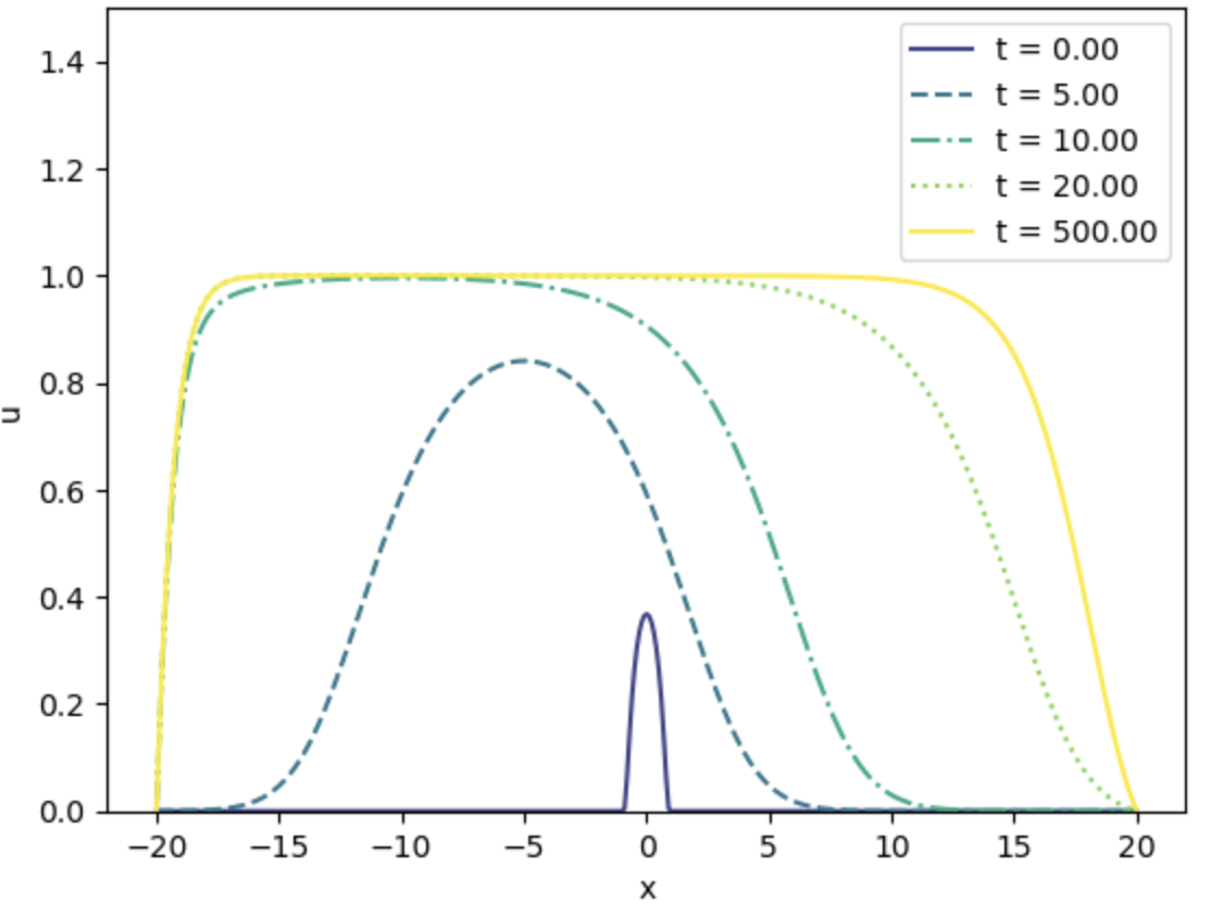
(a) $\chi=1,c=1,u(t,x)$

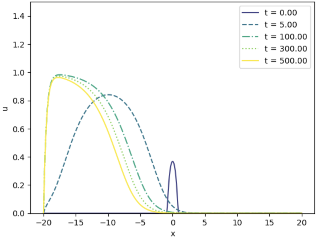
(b) $\chi=1,c=1.99,u(t,x)$

Figure 1:

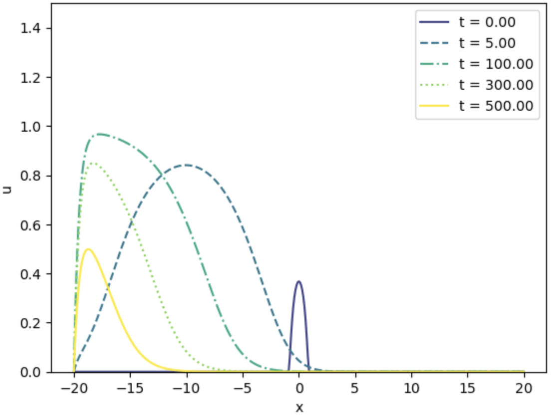
(a) $\chi=1,c=2.01,u(t,x)$

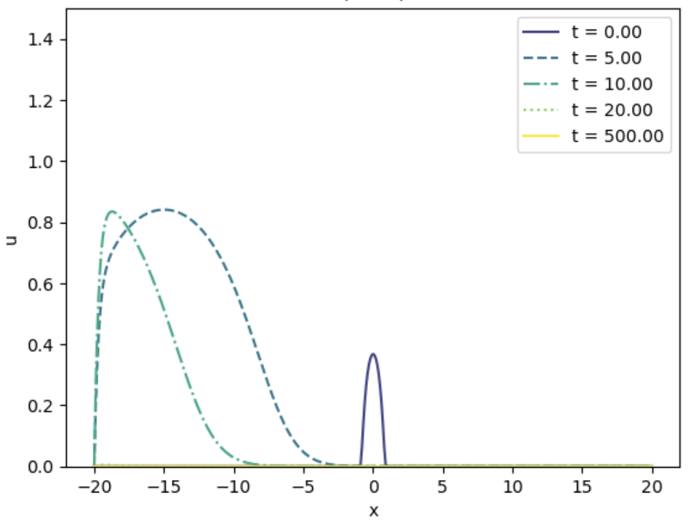
(b) $\chi=1,c=3,u(t,x)$

Figure 2:

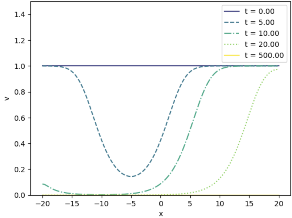
(a) $\chi=1,c=1,v(t,x)$

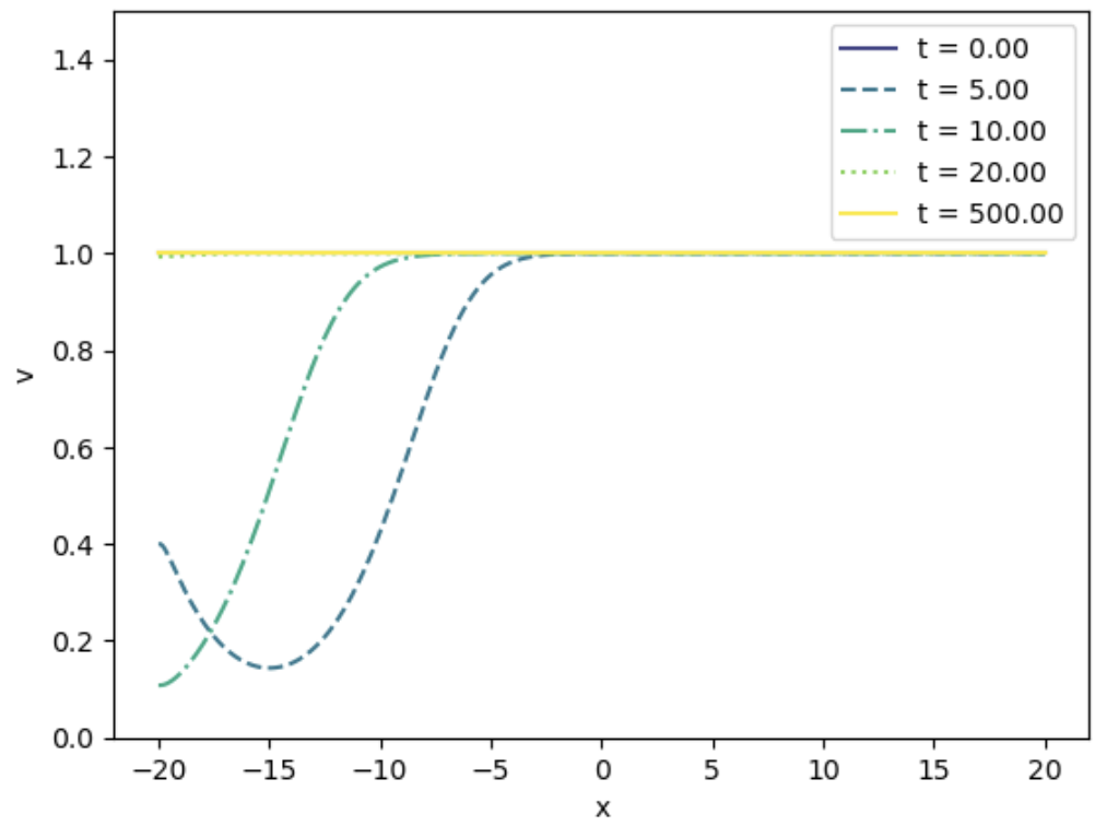
(b) $\chi=1,c=3,v(t,x)$

Figure 3:

We observe the following scenarios via the numerical simulations: The results of the numerical simulations with $\chi=1.25$ and $\chi=1.5$ are similar to those with $\chi=1$. The results show that when $\tilde{u}(t,x)$ stays positive, $\tilde{v}(t,x)\to 0$ as $t\to\infty$, and when $\tilde{u}(t,x)\to 0$, $\tilde{v}(t,x)$ stays positive as $t\to\infty$ (we do not include all the graphs of the $v$-component since we can infer the behavior of $v$ from $u$). For $0<c<2$, $u(t,x)$ stays positive, and for $c>2$, $u(t,x)$ goes to $0$ as $t\to\infty$, which indicates that chemotaxis with a positive but not large sensitivity coefficient $\chi$ does not speed up the spreading.

6.2 Numerical experiments with positive and large $\chi$ and observations

We carry out some numerical experiments with $\chi=2.5,5$ and $\chi=10$. For each of these $\chi$, we do simulations for the following values of $c$, $c=1,1.99,2.01,3$. Figures 4-5 are the graphs of the $u$-component of the numerical solutions of (1.23)+(1.24)+(1.26) with $\chi=10$, and $c=1,1.99,2.01,3$.

We observe that the results of numerical simulations with $\chi=2.5$ and $\chi=5$ are similar to those with $\chi=10$. We also observe that $\tilde{u}(t,x)$ stays positive and $\tilde{v}(t,x)\to 0$ for $c<2$ as well as for $c=2.01$ as $t\to\infty$, which indicates that chemotaxis with positive large sensitivity coefficient $\chi$ speeds up the spreading.

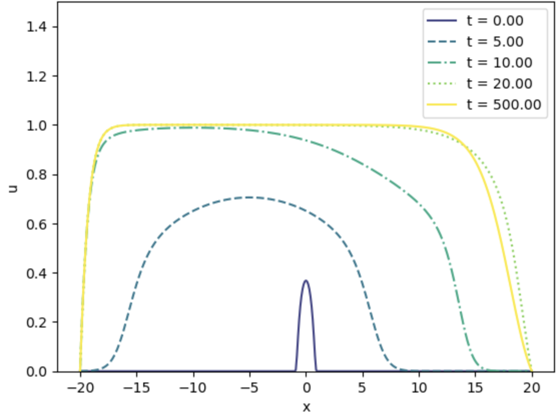
(a) $\chi=10,c=1,u(t,x)$

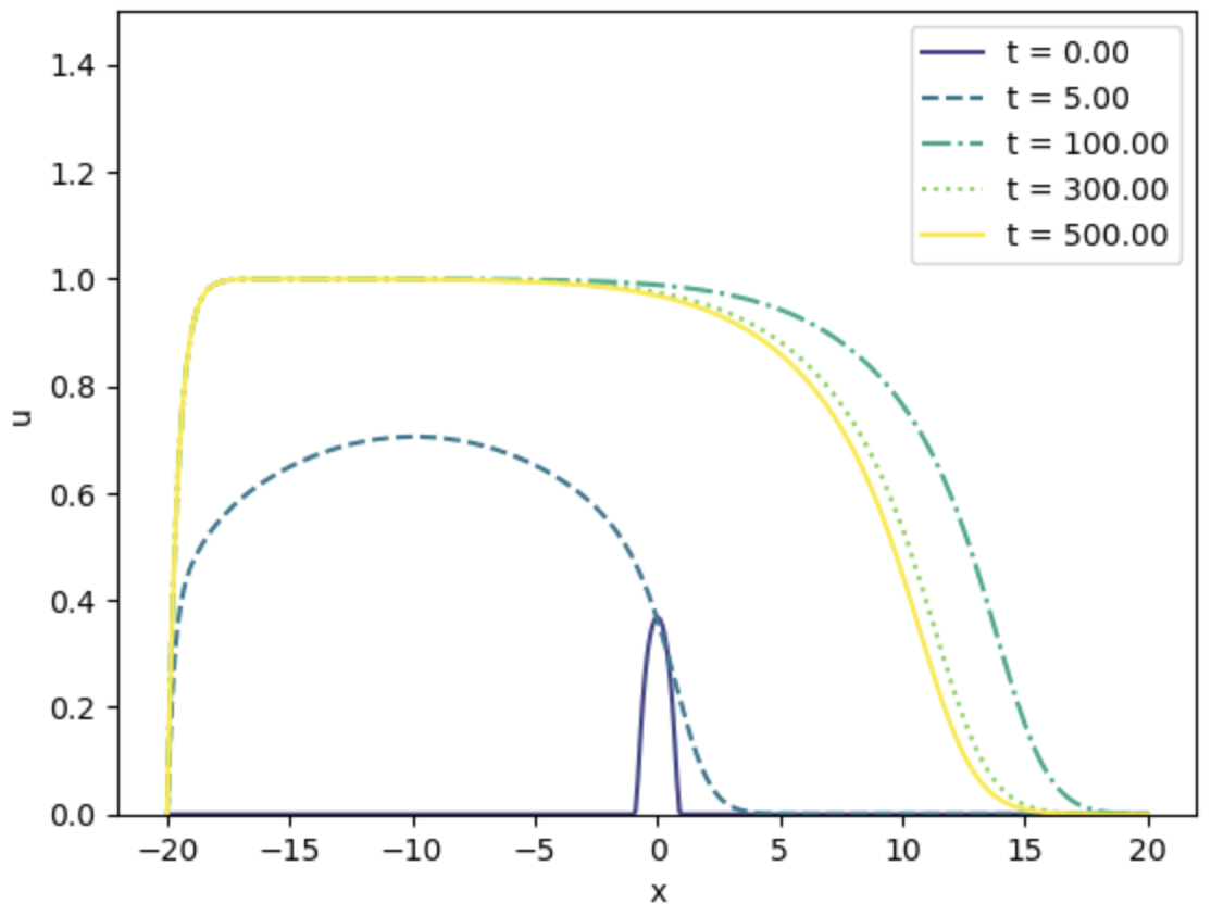
(b) $\chi=10,c=1.99,u(t,x)$

Figure 4:

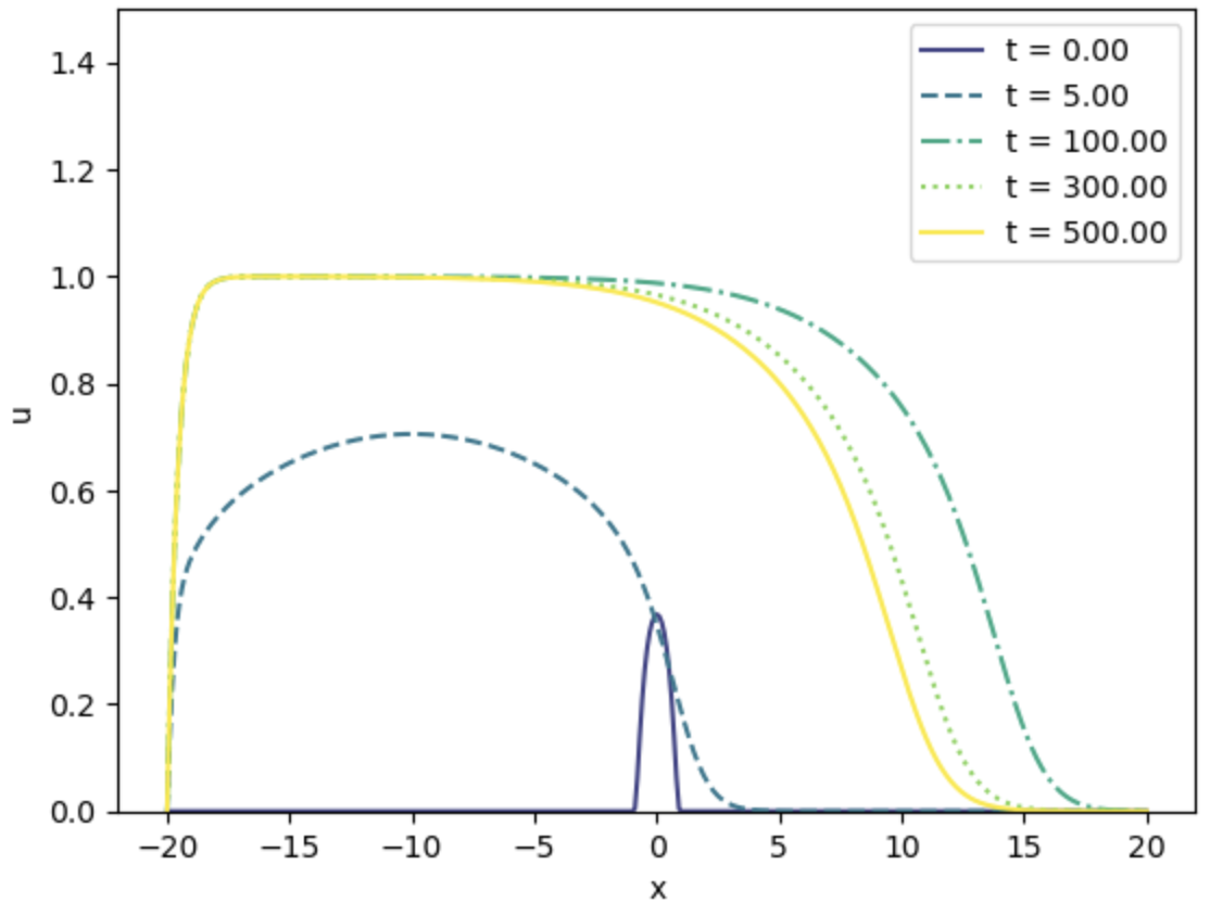
(a) $\chi=10,c=2.01,u(t,x)$

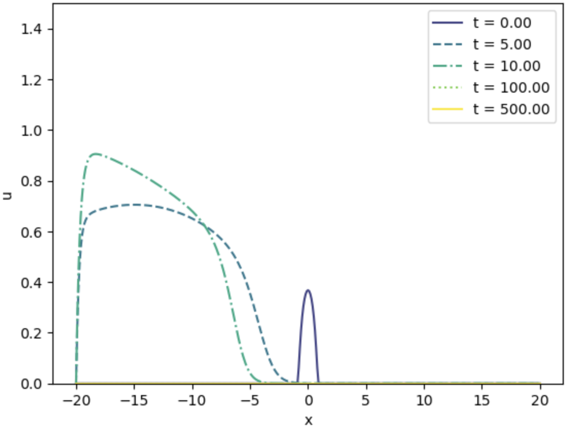
(b) $\chi=10,c=3,u(t,x)$

Figure 5:

6.3 Numerical experiments with negative $\chi$ and observations

We carry out numerical simulations with $\chi=-1$ and $\chi=-10$. For each of theses $\chi$, we do simulations for the following values of $c$, $c=1,1.99,2.01,3$. Figures 6 and 7 are the graphs of the $u$-component of the numerical solutions of (1.23)+(1.24)+(1.26) for $\chi=-1$, and Figures 8 and 9 are the numerical solutions of (1.23)+(1.24)+(1.26) for $\chi=-10$.

We observe that $\tilde{u}(t,x)$ stays positive and $\tilde{v}(t,x)\to 0$ as $t\to\infty$ for $0<c<2$ and $\tilde{u}(t,x)\to 0$ and $\tilde{v}(t,x)$ stays positive as $t\to\infty$, which indicates that chemotaxis with negative sensitivity coefficient or chemo-repeller does not speed up the spreading.

We give the following remarks on all experiments discussed in sections (6.1)–(6.3).

Remark 6.1.

1. The simulations indicate a critical point for $\chi$, i.e there exists $\chi^{*}$ between 1.5 and 1.9 such that for $\chi<\chi^{*}$, the chemotaxis does not speed up the rate of spread, while for $\chi>\chi^{*}$, The chemotaxis speeds up the spreading.

2. For $c=3$, $u(t,x)\to 0$ for all the values of $\chi$. This also supports the fact $c^{*}_{\rm up}<\infty$.

3. In the above numerical experiments, we used the same space step size $h=0.1$ and the same time step size $\tau^{*}=0.002$ as they satisfy the numerical stability condition $\tau/h^{2}<0.5$. We do not give the accuracy analysis of the simulations in this paper. To assess the reliability of the numerical results, we used different values of $h$ and $\tau^{*}$ to simulate the spreading speed of the chemotaxis system in ${\mathbb{R}}$. We repeat the above experiments for $h=0.1$ and $\tau^{*}=0.002,0.004$ and for $\tau^{*}=0.002$ and $h=0.2$. The observed outcomes are close for the different values of $h$ and $\tau^{*}$.

(a) $\chi=-1,c=1,u(t,x)$

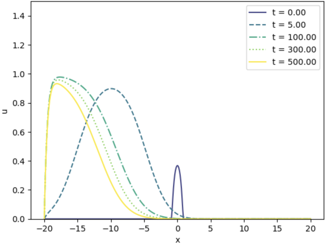
(b) $\chi=-1,c=1.99,u(t,x)$

Figure 6:

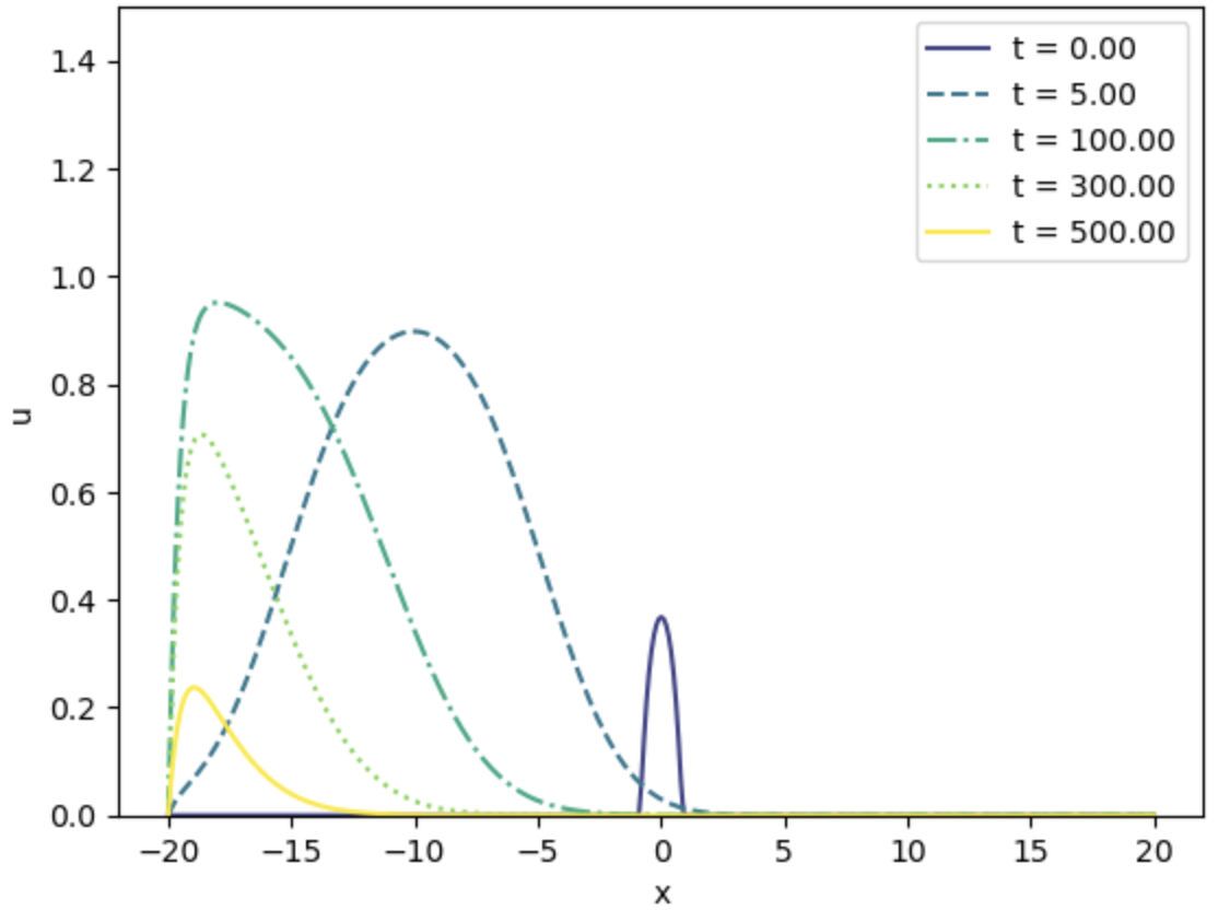
(a) $\chi=-1,c=2.01,u(t,x)$

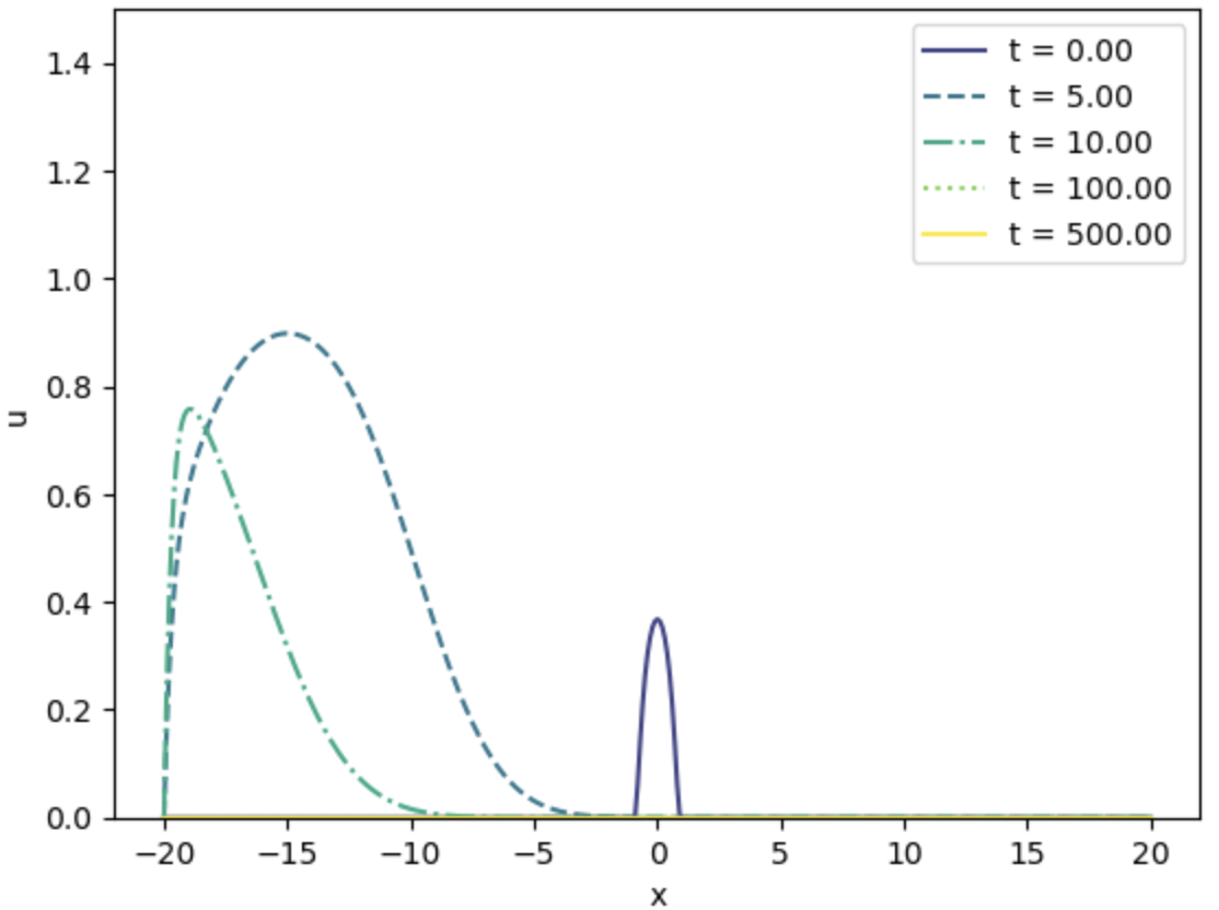
(b) $\chi=-1,c=3,u(t,x)$

Figure 7:

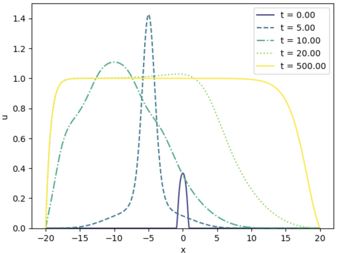
(a) $\chi=-10,c=1,u(t,x)$

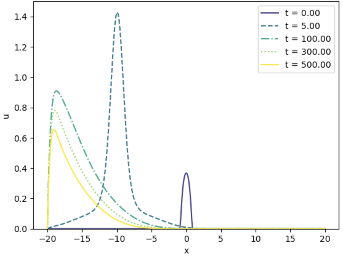
(b) $\chi=-10,c=1.99,u(t,x)$

Figure 8:

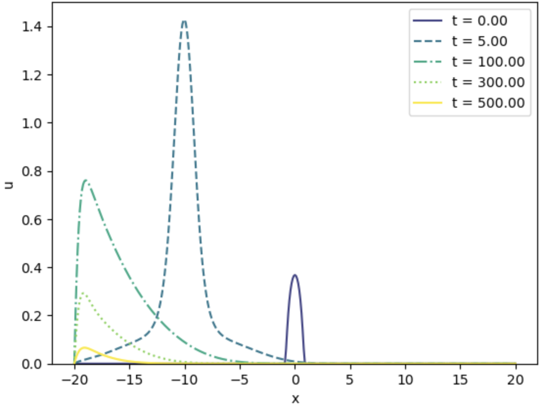
(a) $\chi=-10,c=2.01,u(t,x)$

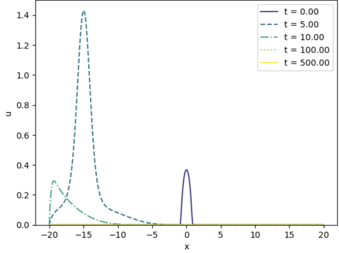
(b) $\chi=-10,c=3,u(t,x)$

Figure 9:

6.4 Numerical Simulations for different $\tau$

We carry out some numerical experiments, to see the effect $\tau$ on the spreading speed. We choose $\tau=0.5$ and $\tau=4$, and $c=1,2.01,3$. The results of the 2D simulations of the $u$-component are shown in subsection 6.4.1-6.4.3 for different time steps. In each of the images, (a) is the result for $\tau=0.5,$ (b) is the result for $\tau=1,$ and $(c)$ is for $\tau=4.$ All the images are for time step $t=0,5,20,500$ except for $c=2.01,\chi=1$, which is for time step $0,4,20,500,1000.$

For $c=2.01,$ we gave the result of the simulation with $\chi=1.9,2.5,5,10$. While for $c=1$ and $c=3,$ we show the result of the simulation for $\chi=1.9,5,10$

6.4.1 Results of simulation for $c=1$

For $c=1$, the solution all stays positive for all $\tau.$ This is expected from Theorem 1.1. The results of the simulations for $\chi=1.9,5,10$ are shown below.

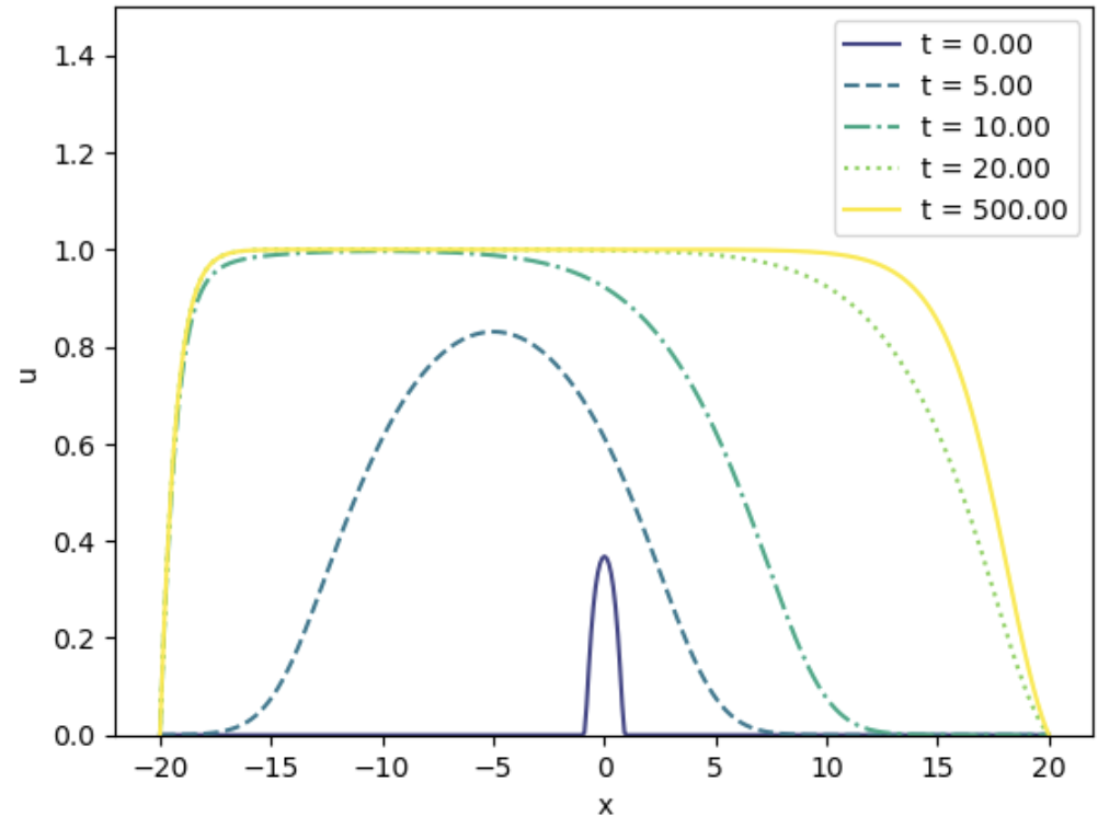
(a)

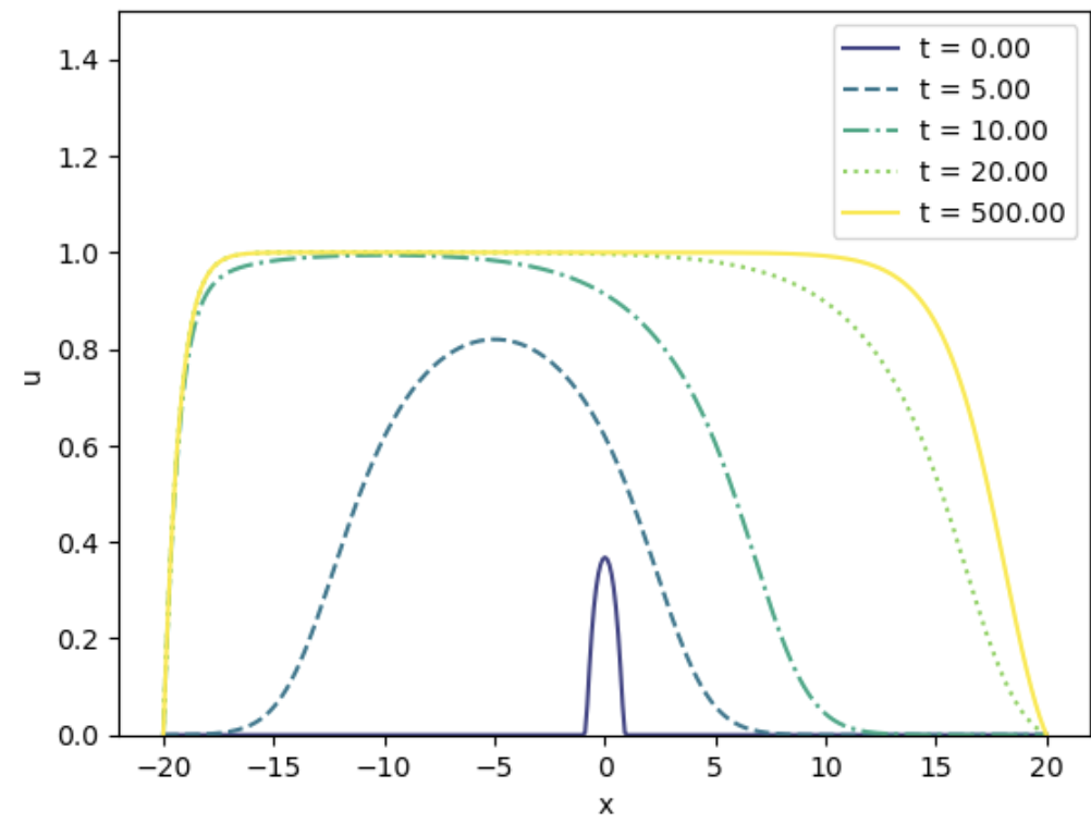
(b)

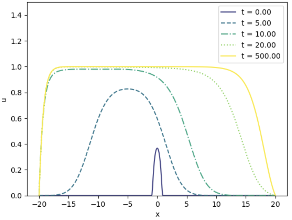
(c)

Figure 10: $\chi=1.9,c=1$

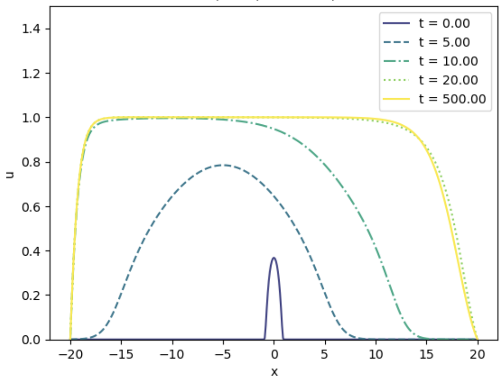
(a)

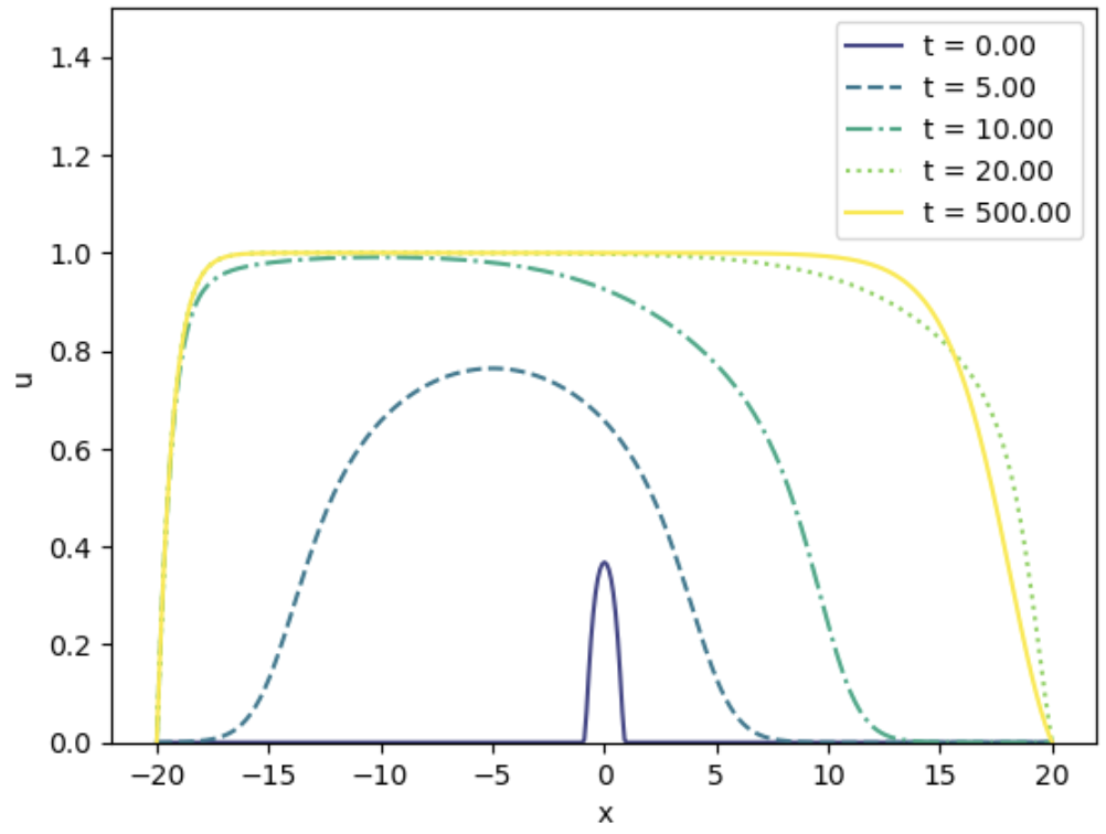
(b)

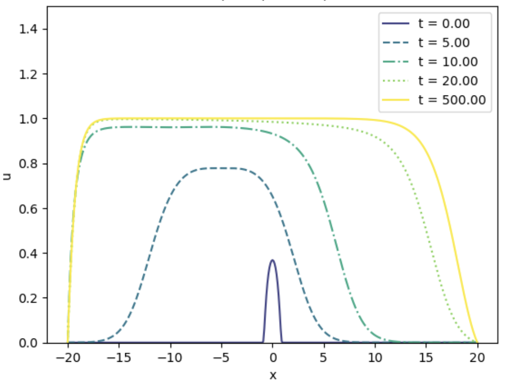
(c)

Figure 11: $\chi=5,c=1$

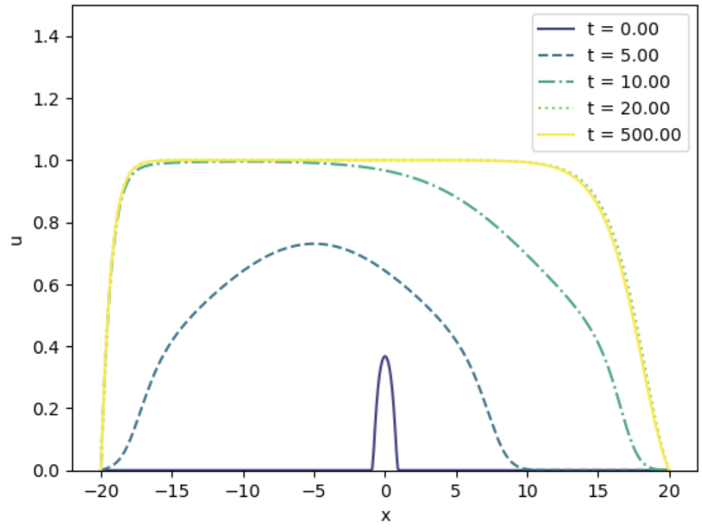
(a)

(b)

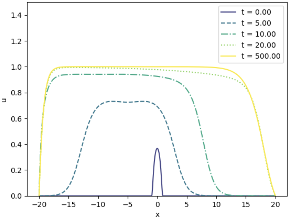
(c)

Figure 12: $\chi=10,c=1$

6.4.2 Results of simulations for $c=2.01$

The result of the simulations shows that the diffusion rate of $v$ has an effect on the spreading speed. We see that as $\tau$ gets bigger, then $u$ goes to zero faster. and the spreading speed interval becomes smaller. We also see that for large $\chi$ there might be speed up for all the $\tau$, as seen for $\chi=5$ and $\chi=10$ in Fig 16 - 17.

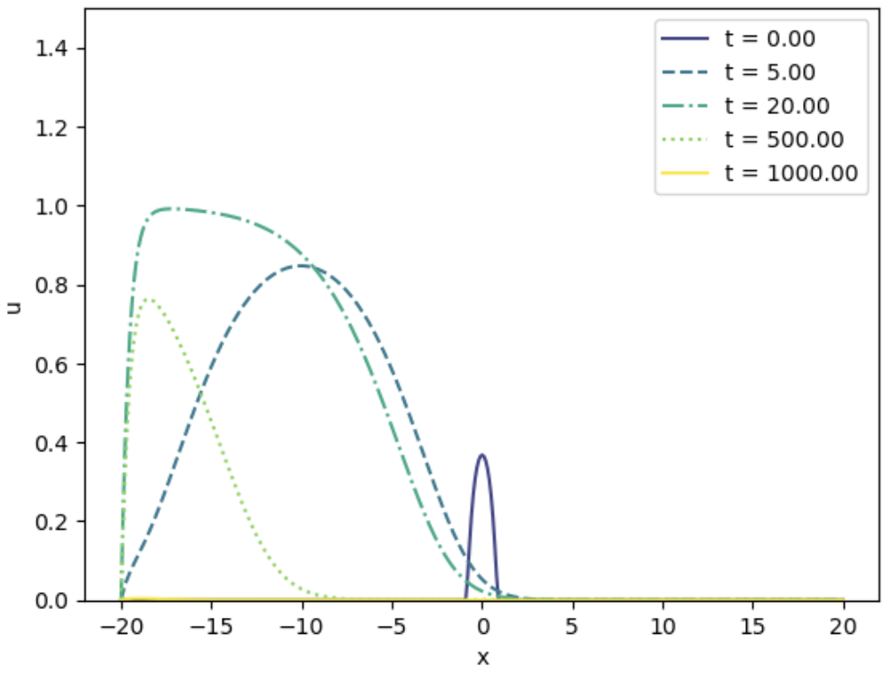
(a)

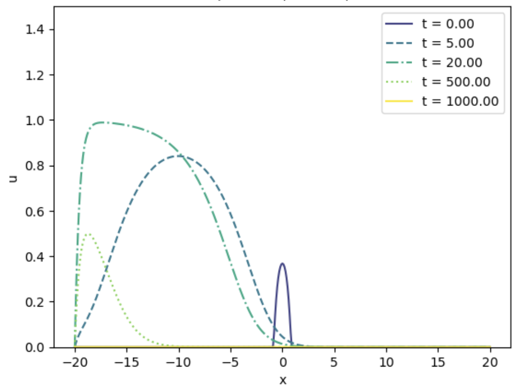
(b)

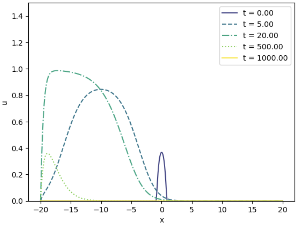
(c)

Figure 13: $\chi=1,c=2.01$

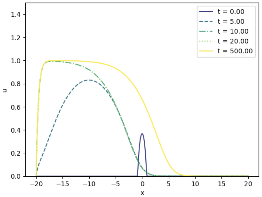
(a)

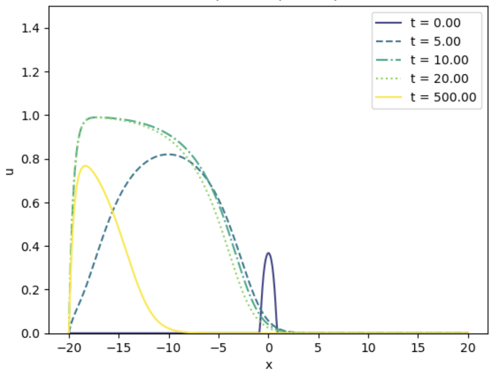
(b)

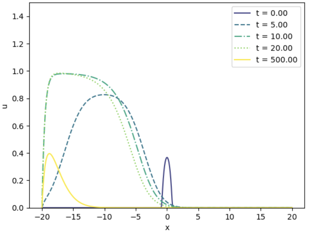
(c)

Figure 14: $\chi=1.9,c=2.01$

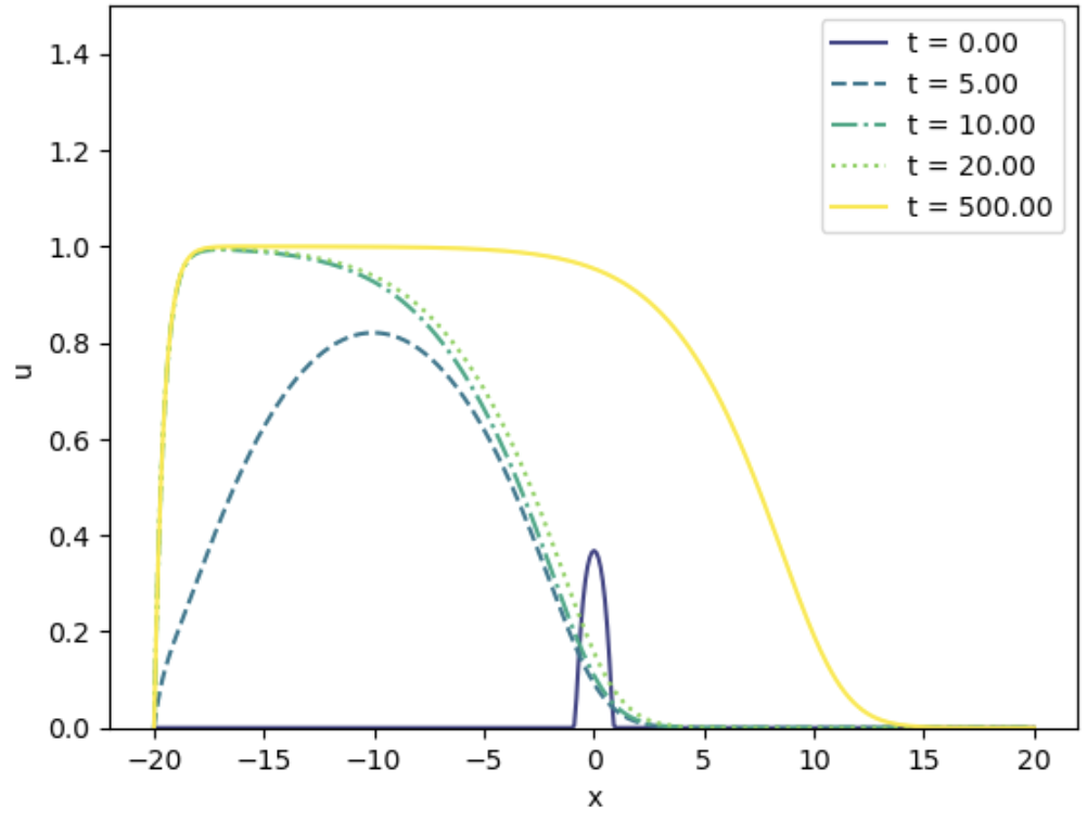
(a)

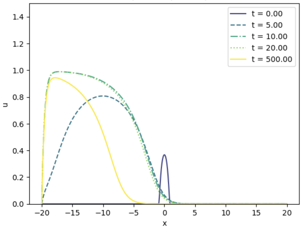
(b)

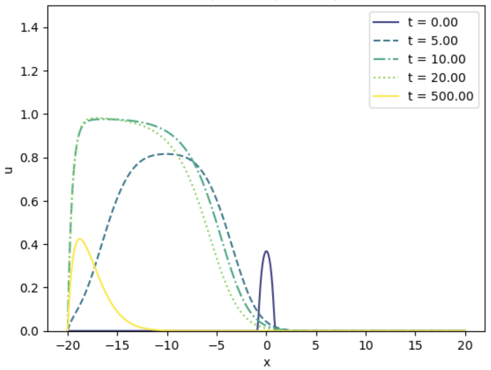
(c)

Figure 15: $\chi=2.5,c=2.01$

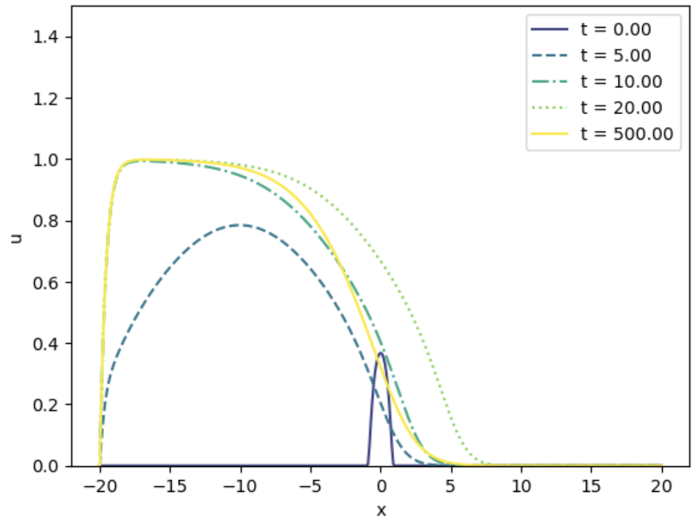
(a)

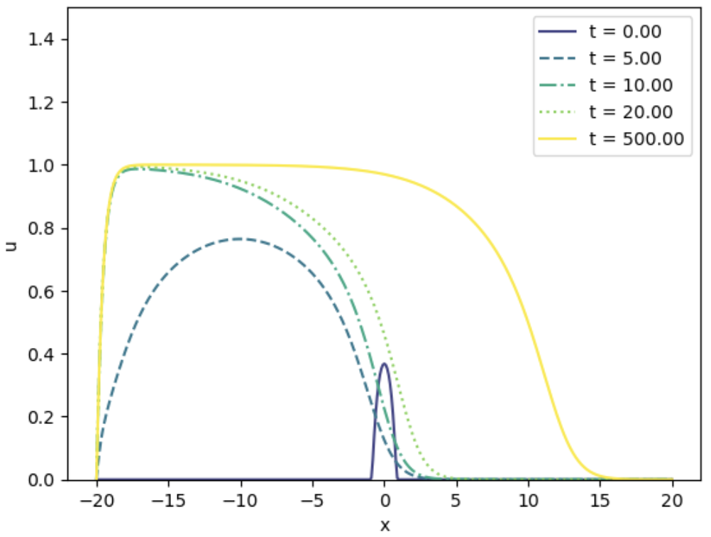
(b)

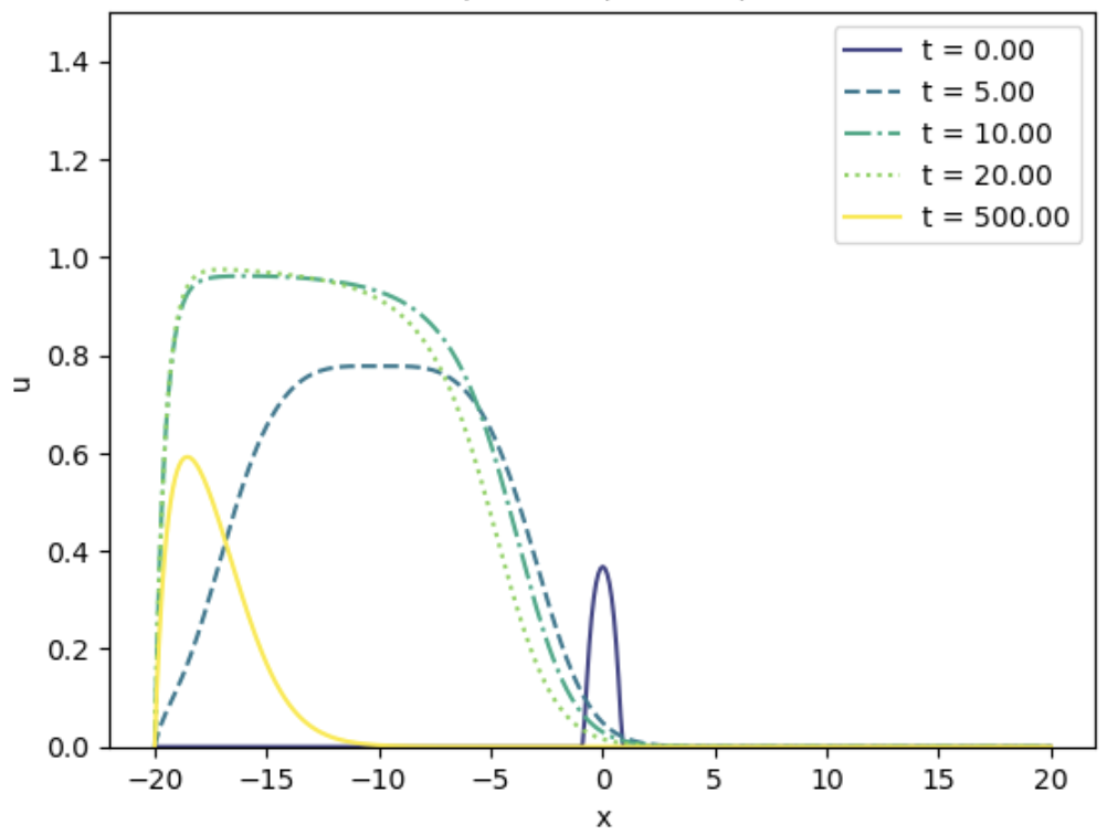
(c)

Figure 16: $\chi=5,c=2.01$

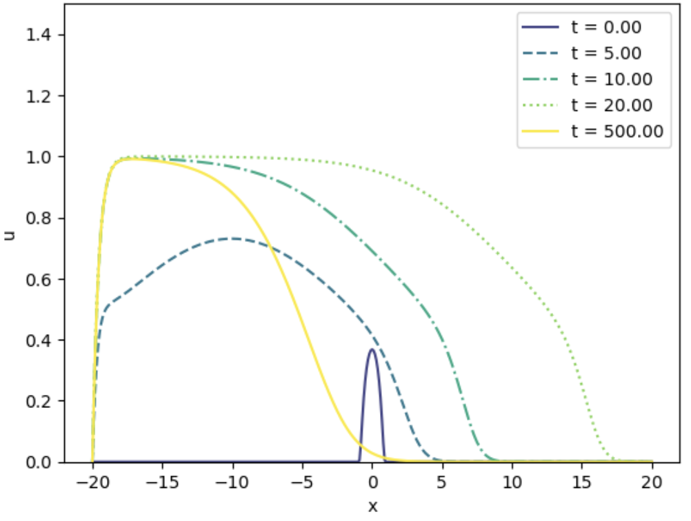
(a)

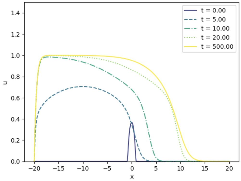
(b)

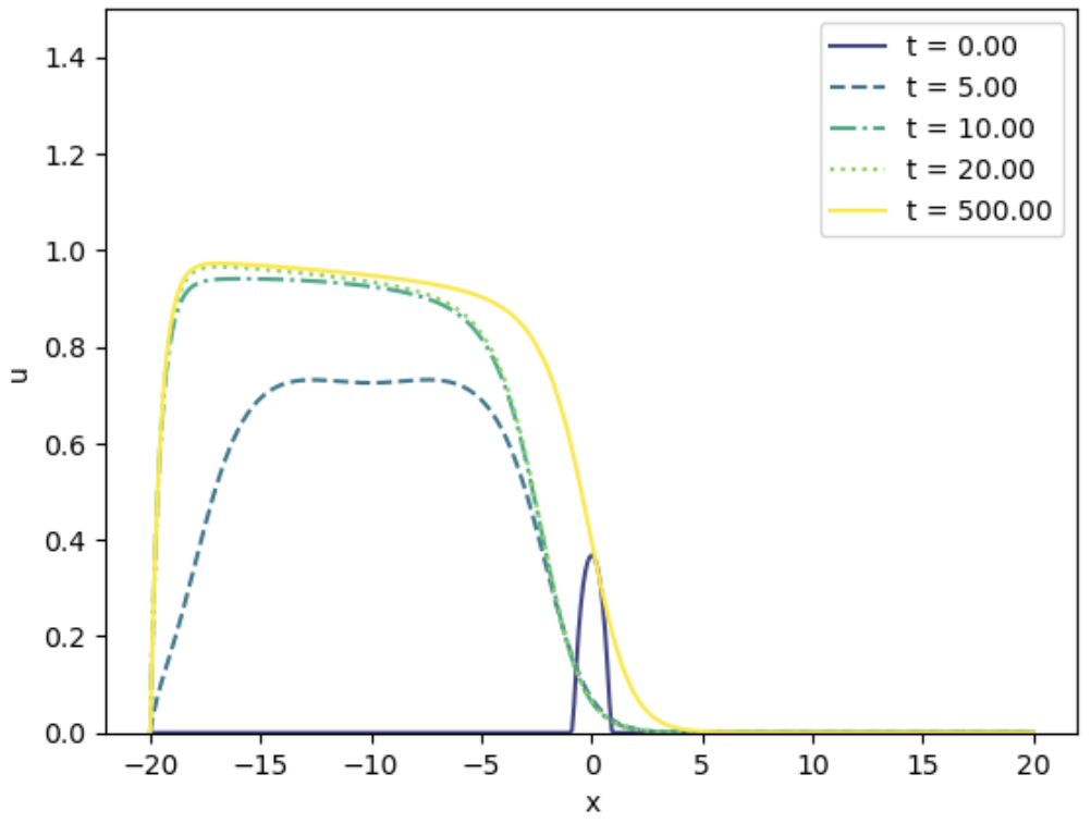
(c)

Figure 17: $\chi=10,c=2.01$

6.4.3 Results of simulation for $c=3$

We carry out the simulation for $c=3$ and $\tau=0.5,1,4$. The results show that the solution goes to zero for large time and for all the $\tau.$

(a)

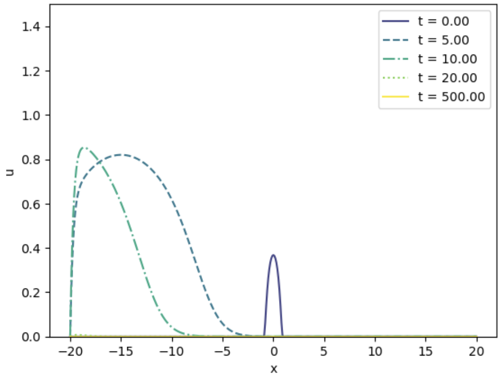
(b)

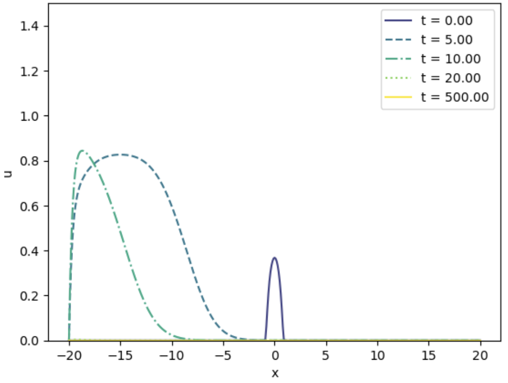
(c)

Figure 18: $\chi=1.9,c=3$

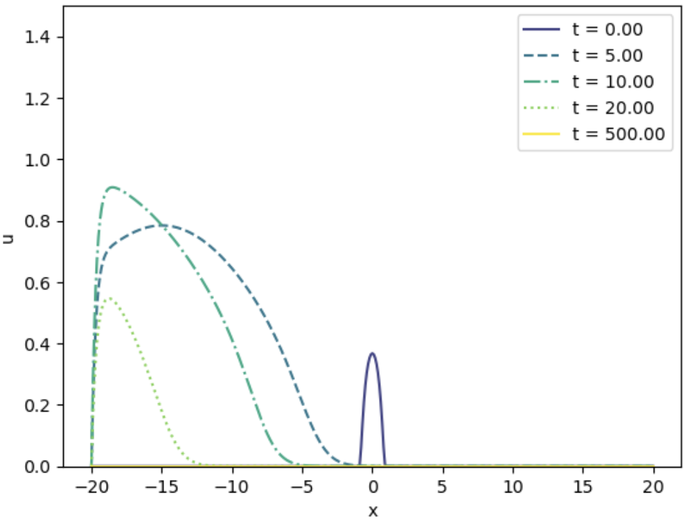
(a)

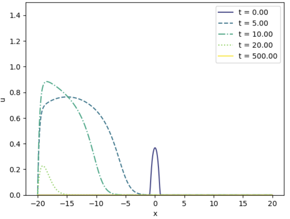
(b)

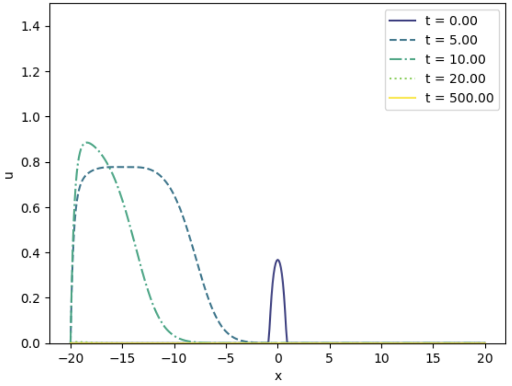
(c)

Figure 19: $\chi=5,c=3$

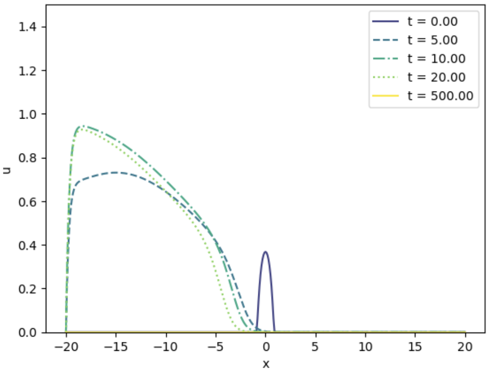
(a)

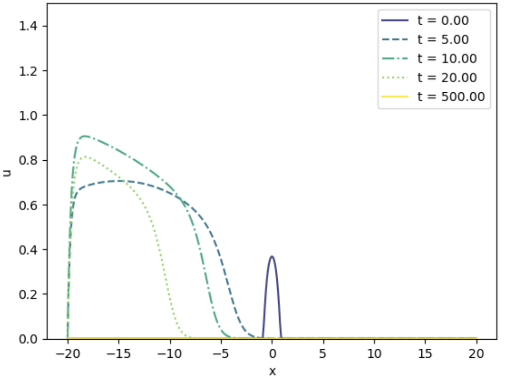
(b)

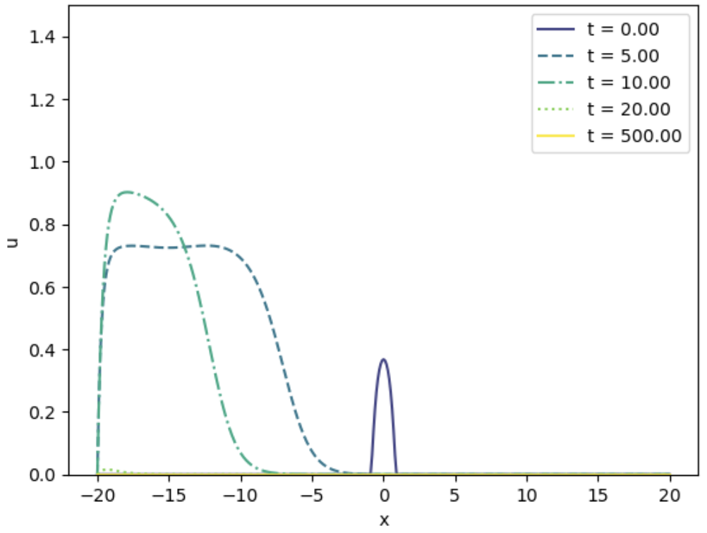
(c)

Figure 20: $\chi=10,c=3$

Appendix A Appendix: Proof of Lemma 2.1

In this appendix, we give a proof of Lemma 2.1.

Proof of Lemma 2.1.

By the boundedness assumption for the solution $(u(t,x),v(t,x))=(u(t,x;u_{0},v_{0})$, $v(t,x;u_{0},v_{0}))$ and a priori estimate for parabolic equations, we have

$$A:=\sup_{t>1}\left(\|\nabla v(t,\cdot)\|_{\infty}+\|\Delta v(t,\cdot)\|_{\infty}\right)<\infty.$$

Note that $A=A(\|v_{0}\|_{\infty},\|u\|_{\infty}).$

We first prove (2.3). To this end, for given $t_{0}\geq 1$, let $t_{1}:=t_{0}-\frac{1}{2}$ and let $\bar{u}(t,x)$ be the solution of the equation

$$\begin{cases}\bar{u}_{t}=\Delta\bar{u}-\chi\nabla v(t,x)\cdot\nabla\bar{u},\qquad&(t,x)\in(t_{1},\infty)\times{\mathbb{R}}^{N},\\ \bar{u}(t_{1},\cdot)=u(t_{1},\cdot),&x\in{\mathbb{R}}^{N}.\end{cases}$$

It follows from the comparison principle for parabolic equations that

$$0\leq\bar{u}(t,x)\leq\|u(t_{1},\cdot)\|_{\infty}\leq\|u\|_{\infty}:=\sup_{s\geq 0}\|u(s,\cdot)\|_{\infty}\quad\forall\,(t,x)\in(t_{1},\infty)\times{\mathbb{R}}^{N}.$$

Let $\psi(t,x)$ and $\phi(t,x)$ be defined by

$$\psi(t,x)=\min\big{\{}1,({a}/{b})^{1/\sigma}/\|u\|_{\infty}\big{\}}\,e^{-|\chi|A(t-t_{1})}\,\bar{u}(t,x)$$ (A.1)

and

$$\phi(t,x)=e^{(a+A|\chi|)(t-t_{1})}\,\bar{u}(t,x),$$

respectively. Then, we have for $(t,x)\in(t_{1},\infty)\times{\mathbb{R}}^{N}$,

$$\psi_{t}=-|\chi|A\psi+\Delta\psi-\chi\nabla v\cdot\nabla\psi\leq\Delta\psi-\chi\nabla\cdot(\psi\nabla v)\leq\Delta\psi-\chi\nabla\cdot(\psi\nabla v)+\psi(a-b\psi^{\sigma}),$$

and

$$\phi_{t} =(a+|\chi|A)\phi+\Delta\phi-\chi\nabla v\cdot\nabla\phi\geq\Delta\phi-\chi\nabla\cdot(\phi\nabla v)+a\phi$$

$$\geq\Delta\phi-\chi\nabla\cdot(\phi\nabla v)+\phi(a-b\phi^{\sigma}).$$

Since

$$\psi(t_{1},\cdot)\leq\phi(t_{1},\cdot)=\bar{u}(t_{1},\cdot)=u(t_{1},\cdot),$$

the comparison principle yields

$$\psi(t,\cdot)\leq u(t,\cdot)\leq\phi(t,\cdot)\quad\forall\,t\geq t_{1}.$$

Note that

$$\bar{u}(t,x)=\int_{{\mathbb{R}}^{N}}\Gamma(t,t_{1},x,z)u(t_{1},z)dz,$$

where $\Gamma(t,t_{1},x,z)$ is the fundamental solution of the equation

$$\begin{cases}\Gamma_{t}=\Delta_{x}\Gamma-\chi\nabla_{x}v\cdot\nabla_{x}\Gamma,\qquad\qquad\text{ for }(t,x)\in(s,\infty)\times{\mathbb{R}}^{N},\\ \Gamma(t=t_{1},t_{1},x,z)=\delta_{z}(x).\end{cases}$$

Hence

$$\min\left\{1,({a}/{b})^{1/\sigma}/\|u\|_{\infty}\right\}\,e^{-|\chi|A(t-t_{1})}\int_{{\mathbb{R}}^{N}}\Gamma(t,t_{1},x,z)u(t_{1},z)dz\leq u(s^{\prime},x)$$ (A.2)

$$\qquad\qquad\leq e^{(a+A|\chi|)(t-t_{1})}\int_{{\mathbb{R}}^{N}}\Gamma(t,t_{1},x,z)u(t_{1},z)dx\quad\forall\,t\geq t_{1},\,\,x\in{\mathbb{R}}^{N}.$$

Let $p>1$, $q$ be the conjugate exponent to $p$ and let $\alpha:=(1+p)/(2p)$. From the proof of [10, (4.25)], for any fixed $s_{0},R>0$, there exists a constant $C_{0}>0$ depending only on $s_{0}$, $R$, $p$, $A$, $N$ and an upper bound of $|\chi|$ such that

$$\Gamma(t_{0},t_{1},x,z)^{\alpha p}\leq C_{0}\,\Gamma(t,t_{1},y,z)\,\,\forall\,t\in[t_{0},t_{0}+s_{0}],\,\,|x-y|\leq R,\,\,z\in{\mathbb{R}}^{N}.$$ (A.3)

By [1, Theorem 10], there exists $C_{1}\geq 1$, depending only $\chi$, $A$ and $N$, such that for any $x,y\in{\mathbb{R}}^{N}$ and $0\leq s<t$ with $t-s\leq\frac{1}{2}$,

$$({C_{1}(t-s)^{N/2}})^{-1}e^{-C_{1}\frac{|x-y|^{2}}{t-s}}\leq\Gamma(t,s,x,y)\leq{C_{1}}{(t-s)^{-N/2}}e^{-\frac{|x-y|^{2}}{C_{1}(t-s)}}.$$

This and $t_{0}=t_{1}+\frac{1}{2}$ imply that there is $C_{2}(q,\chi,N)$ such that

$$\|\Gamma(t_{0},t_{1},x,\cdot)^{1-\alpha}\|_{q}\leq C_{2}\quad\forall\,x\in{\mathbb{R}}^{N}.$$ (A.4)

By (A.2) and Hölder’s inequality, we have

$$u(t_{0},x) \leq e^{(a+A|\chi|)/2}\int_{{\mathbb{R}}^{N}}\Gamma(t_{0},t_{1},x,z)\,u(t_{1},z)\,dz$$

$$\leq e^{(a+A|\chi|)/2}\,\|u\|_{\infty}^{1/q}\int_{{\mathbb{R}}^{N}}\left(u(t_{1},z)\,\Gamma(t_{0},t_{1},x,z)^{\alpha p}\right)^{1/p}\Gamma(t_{0},t_{1},x,z)^{(1-\alpha)}dz$$

$$\leq e^{(a+A|\chi|)/2}\,\|u\|_{\infty}^{1/q}\,\|\Gamma(t_{0},t_{1},x,\cdot)^{1-\alpha}\|_{q}\left(\int_{{\mathbb{R}}^{N}}u(t_{1},z)\Gamma(t_{0},t_{1},x,z)^{\alpha p}dz\right)^{1/p}.$$

Using (A.3) and (A.4) yields for $t\in[t_{0},t_{0}+s_{0}]$,

$$u(t_{0},x) \leq C_{2}C_{0}^{1/p}e^{(a+A|\chi|)/2}\,\|u\|_{\infty}^{1/q}\,\left(\int_{{\mathbb{R}}^{N}}u(t_{1},z)\Gamma(t,t_{1},y,z)dz\right)^{1/p}$$

$$\leq C_{2}C_{0}^{1/p}e^{(a+A|\chi|)/2+|\chi|A(\frac{1}{2}+s_{0})/p}\max\left\{\|u\|_{\infty}^{1/q},\|u\|_{\infty}\left({b}/{a}\right)^{1/(\sigma p)}\right\}u(t,y)^{1/p},$$

where in the last inequality, we applied (A.2). We can conclude with (2.3).

Next, we prove (2.4). By a priori estimate for parabolic equations (see [28, Theorem 7.22]) and the anisotropic Sobolev embedding for $q=N+3$ (see [6, Lemma A3]), there is $C_{3}=C_{3}(A,\chi,R,N)>0$ such that for any $(t,x)\in(1,\infty)\times{\mathbb{R}}^{n}$,

$$\begin{split}|\nabla u(t,x)|&\leq C_{3}\,\left(\|u\|_{L^{q}([t-\frac{1}{2},t]\times B_{R}(x))}+\|u(a-bu)\|_{L^{q}([t-\frac{1}{2},t]\times B_{R}(x))}\right)\\ &\leq C_{3}\,\|u\|_{L^{\infty}([t-\frac{1}{2},t]\times B_{R}(x))}\,(1+a+b\|u\|_{\infty}).\end{split}$$

By (2.3), for any $p\in(1,\infty)$, there exists a constant $C>0$ that depends only on $a$, $b$, $R$, $p$, $A$, $\chi$, $N$, and $\|u\|_{\infty}$ such that

$$|\nabla u(t,x)|\leq{C\,u(t,y)^{1/p}}$$

for all $|x-y|\leq R$, which proves (2.4). ∎

References

- [1] D. G. Aronson, Non-negative solutions of linear parabolic equations, Ann. Scuola Norm. Sup. Pisa (3) 22 (1968), 607-69.
- [2] D. G. Aronson, H. F. Weinberger, Nonlinear diffusion in population genetics, combustion, and nerve pulse propagation, in Partial Differential Equations and Related Topics, ed. J.A. Goldstein. Lecture Notes in Mathematics 446 (1975), 5-49.
- [3] D. G. Aronson and H. F. Weinberger, Multidimensional nonlinear diffusions arising in population genetics, Adv. in Math., 30 (1978), pp. 33-76.
- [4] J. Bramburger, Exact minimum speed of traveling waves in a Keller-Segel model, Appl. Math. Lett. 111 (2021), Paper No. 106594, 7 pp.
- [5] M. G. Crandall, H. Ishii and P.-L. Lions, User’s guide to viscosity solutions of second order partial differential equations, Bull. Amer. Math. Soc. (N.S.), 27 (1992), no. 1, 1–67.
- [6] H. Engler, Global smooth solutions for a class of parabolic integrodifferential equations, Trans. Amer. Math. Soc. 348 (1996), 267-290.
- [7] R. Fisher, The wave of advance of advantageous genes, Ann. of Eugenics, 7 (1937), 355-369.
- [8] H. I. Freedman, X.-Q. Zhao, Global asymptotics in some quasimonotone reaction-diffusion systems with delay, J. Differential Equations 137 (1997), 340-362.
- [9] Q. Griette, C. Henderson, and O. Turanova, Speed-up of traveling waves by negative chemotaxis, Journal of Functional Analysis, 285 (2023), no. 10, 110115.
- [10] F. Hamel and C. Henderson, Propagation in a Fisher-KPP equation with non-local advection, J. Funct. Anal. 278 (2020), no. 7, 108426, 53 pp.
- [11] Z. Hassan, W. Shen, Y. P. Zhang, Global existence of classical solutions of chemotaxis systems with logistic source and consumption or linear signal production on .
- [12] C. Henderson, Slow and fast minimal speed traveling waves of the FKPP equation with chemotaxis, J. Math. Pures Appl. (9)167 (2022), 175-203.
- [13] C. Henderson and M. Rezek, Traveling waves for the Keller-Segel-FKPP equation with strong chemotaxis, J. Differential Equations, 379 (2024), 497-523.
- [14] D. Henry, Geometric theory of semilinear parabolic equations, vol. 840 of Lecture Notes in Mathematics, Springer-Verlag, Berlin-New York, 1981.
- [15] M. A. Herrero and J. J. L. Velázquez, Singularity patterns in a chemotaxis model, Math. Ann. 306 (1996), 583-623.
- [16] M. A. Herrero and J. J. L. Velázquez, A blow-up mechanism for a chemotaxis model, Ann. Scuola Norm. Sup. Pisa Cl. Sci., (4) 24 (1997), no.4, 633-683.
- [17] T. B. Issa and W. Shen, Pointwise persistence in full chemotaxis models with logistic source on bounded heterogeneous environments, J. Math. Anal. Appl., 490, (2020) 124204.
- [18] W. Jager and S. Luckhaus, On explosions of solutions to a system of partial differential equations modelling chemotaxis, Trans. Amer. Math. Soc. 329 (1992), 819-824.
- [19] E. F. Keller and L. A. Segel, Initiation of some mold aggregation viewed as an instability, J. Theor. Biol. 26, (1970), 399-415.
- [20] E. F. Keller and L. A. Segel, Traveling bands of chemotactic bacteria: a theoretical analysis, J. Theor. Biol. 30 (1971), 377-380.
- [21] E. F. Keller and L. A. Segel, A Model for chemotaxis, J. Theoret. Biol., 30 (1971), 225-234.
- [22] I. Kim and Y. P. Zhang, Porous medium equation with a drift: Free boundary regularity, Arch. Ration. Mech. Anal., 242 (2021), no. 2, 1177–1228.
- [23] I. Kim and Y. P. Zhang, Regularity of Hele-Shaw Flow with source and drift, arXiv preprint arXiv:2210.14274, (2022).
- [24] A. Kolmogorov, I. Petrowsky, and N.Piscunov, A study of the equation of diffusion with increase in the quantity of matter, and its application to a biological problem, Bjul. Moskovskogo Gos. Univ., 1 (1937), 1-26.
- [25] J. Lankeit and Y. Wang, Global existence, boundedness and stabilization in a high-dimensional chemotaxis system with consumption, Discrete Contin. Dyn. Syst. 37 (2017), no. 12, 6099-6121.
- [26] T. Li and J. Park, Traveling waves in a Keller-Segel model with logistic growth, Commun. Math. Sci. 20 (2022), no.3, 829-853.
- [27] T. Li and Z.-A. Wang, Traveling wave solutions of a singular Keller-Segel system with logistic source, Math. Biosci. Eng. 19 (2022), no.8, 8107-8131.
- [28] G. M. Lieberman, Second order parabolic differential equations, World Scientific Publishing Co., Inc., River Edge, NJ, 1996.
- [29] T. Nagai, Blow-up of radially symmetric solutions to a chemotaxis system, Adv. Math. Sci. Appl. (1995), 1-21.
- [30] K. Osaki, T. Tsujikawa, A. Yagi and M. Mimura, Exponential attractor for a chemotaxis-growth system of equations, Nonlinear Anal. TMA 51(2002), 119-144.
- [31] K. Osaki and A. Yagi, Finite dimensional attractors for one-dimensional Keller-Segel equations, Funkcialaj Ekvacioj, 44 (2001), 441-469.
- [32] R. B. Salako and W. Shen, Global existence and asymptotic behaviour of solution in parabolic-elliptic chemotaxis system with logistic source, Jounal of Differential Equation 262(2017) 5635-5690.
- [33] R. B. Salako and W. Shen, Existence of Traveling wave solution of parabolic-parabolic chemotaxis systems, Nonlinear Analysis: Real World Applications Volume 42, (2018), 93-119.
- [34] R. B. Salako and W. Shen, Spreading Speeds and Traveling waves of a parabolic-elliptic chemotaxis system with logistic source on , Discrete and Continuous Dynamical Systems - Series A, 37 (2017), pp. 6189-6225.
- [35] R. B. Salako and W. Shen, Global existence and asymptotic behavior of classical solutions to a parabolic-elliptic chemotaxis system with logistic source on , J. Differential Equations, 262 (2017) 5635-5690.
- [36] R. B Salako, W. Shen, S. Xue, Can chemotaxis speed up or slow down the spatial spreading in parabolic-elliptic Keller-Segel systems with logistic source? J. Math. Biol., 79 (2019), 1455-Ai1490.
- [37] W. Shen and S. Xue, Spreading speeds of a parabolic - parabolic chemotaxis model with logistic source of , J. Math. Anal. Appl. 475 (2019), no. 1, 895-917.
- [38] Y. Tao, Boundedness in a chemotaxis model with oxygen consumption by bacteria, J. Math. Anal. Appl. 381 (2011), 521-529.
- [39] L. Wang, Shahab Ud-Din Khan, and Salah Ud-Din Khan, Boundedness in a chemotaxis system with consumption of chemoattractant and logistic source, Electron. J. Differential Equations (2013), no. 209, pp. 9.
- [40] Y. Wang and C. Ou, New results on traveling waves for the Keller-Segel model with logistic source, Appl. Math. Lett. 145 (2023), Paper No. 108747, 7 pp.
- [41] M. Winkler, Boundedness in the higher-dimensional parabolic-parabolic chemotaxis system with logistic source, Communications in Partial Differential Equations, 35(8) (2010), 1516-1537.
- [42] Q. Zhang and Y. Li, Stabilization and convergence rate in a chemotaxis system with consumption of chemoattractant, J. Math. Phys. 56 (2015), no.8, 081506.
- [43] J. Zheng, Y. Y. Li, G. Bao, and X. Zou, A new result for global existence and boundedness of solutions to a parabolic-parabolic Keller-Segel system with logistic source, Journal of Mathematical Analysis and Applications, 462 (2018), 1-25.