Supernova axions convert to gamma-rays in magnetic fields of progenitor stars

Abstract

It has long been established that axions could have been produced through the Primakoff process within the nascent proto-neutron-star formed following the type II supernova SN1987A, escaped the star due to their weak interactions, and then converted to gamma-rays in the Galactic magnetic fields; the non-observation of a gamma-ray flash coincident with the neutrino burst leads to strong constraints on the axion-photon coupling for axion masses $m_{a}\lesssim 10^{-10}$ eV. In this work we use SN1987A to constrain, for the first time, higher mass axions, all the way to $m_{a}\sim 10^{-3}$ eV, by accounting for axion-photon conversion on the still-intact magnetic fields of the progenitor star. Moreover, we show that gamma-ray observations of the next Galactic supernova, leveraging the magnetic fields of the progenitor star, could detect quantum chromodynamics axions for masses above roughly $50$ $\mu$eV, depending on the supernova. We propose a new full-sky gamma-ray satellite constellation that we call the GALactic AXion Instrument for Supernova (GALAXIS) to search for such future signals along with related signals from extragalactic neutron star mergers.

Supernova (SN) 1987A (SN1987A) was a type II SN that exploded in February 1987, producing roughly two dozen neutrino events that were detected at the Kamiokande II, IMB, and Baksan neutrino detectors over a time interval of around 10 s Hirata et al. (1987); Bionta et al. (1987); Alekseev et al. (1987). The SN took place in the Large Magellanic Cloud at a distance of approximately 51.4 kpc from Earth. SN1987A provides some of the most stringent and well-established constraints on a class of hypothetical ultra-light pseudo-scalar particles known as axions Raffelt (1996, 1990); Brockway et al. (1996); Grifols et al. (1996); Payez et al. (2015); Hoof and Schulz (2023); Caputo and Raffelt (2024). These constraints have been made all the more robust recently by the tentative discovery of the NS formed after SN1987A, helping establish that the SN formed a neutron star (NS) and not a black hole Page et al. (2020); Fransson et al. (2024). In this work we point out for the first time a novel constraint from SN1987A that has promising implications for future SN; axions produced within the proto-NS (PNS) can convert to observable gamma-rays in the stellar magnetic field of the progenitor star.

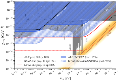
Figure 1: Existing constraints (notably Reynolds et al. (2020); Dessert et al. (2020); Reynés et al. (2021); Noordhuis et al. (2023); Dessert et al. (2022); Dolan et al. (2022); Davies et al. (2023); Ning and Safdi (2024) and O’HARE (2020); Workman and Others (2022) for reviews) on the axion-photon coupling $g_{a\gamma\gamma}$ as a function of the axion mass $m_{a}$ are shaded in grey, with the previously-leading constraint from the non-observation of axion-induced gamma-rays from SN1987A highlighted Payez et al. (2015); Hoof and Schulz (2023). We point out in this work that the axions could convert to gamma-rays in the stellar magnetic field of the progenitor star, extending the upper limit on $g_{a\gamma\gamma}$ to higher masses as indicated in shaded blue. We take the surface field strength of the progenitor to be 100 G to be conservative ($\sim$1 kG is favored). Note that the KSVZ-like axion model assumes the couplings to photons and hadrons are related as in the KSVZ QCD-axion model (see text). The non-observation of gamma-rays from the next Galactic SN (assumed to be at $d=10$ kpc) with the proposed GALAXIS full-sky gamma-ray telescope network (modeled as being equivalent to the on-axis Fermi-LAT instrument response with full-sky coverage) could cover vast regions of QCD axion parameter space (red), depending on the properties of the progenitor star (BSG shown here, assuming a typical 1 kG surface field strength) and the axion.

Axions may address a number of outstanding problems in nature such as the strong-CP problem Peccei and Quinn (1977a, b); Weinberg (1978); Wilczek (1978) (i.e., the lack of a neutron electric dipole moment) and the measured dark matter abundance in the Universe Preskill et al. (1983); Abbott and Sikivie (1983); Dine and Fischler (1983). Moreover, axions are now understood to arise generically in string theory compactifications Svrcek and Witten (2006); Arvanitaki et al. (2010); Cicoli et al. (2012); Demirtas et al. (2020); Halverson et al. (2019); Demirtas et al. (2021). String theory motivates the picture of the ‘axiverse,’ where the quantum chromodynamics (QCD) axion that solves the strong-CP problem is accompanied by a number of axion-like particles, which interact through higher dimensional operators with the rest of the Standard Model but not with QCD. The QCD axions receive a mass contribution from QCD of the order $m_{a}^{\rm QCD}\approx 5.70\,\,{\rm\mu eV}(10^{12}\,\,{\rm GeV}/f_{a})$, with $f_{a}$ the axion decay constant. The axion field $a$ has an interaction with photons ${\mathcal{L}}=g_{a\gamma\gamma}a{\bf E}\cdot{\bf B}$, with ${\bf E}$ (${\bf B}$) the electric (magnetic) field, that is parameterized by the coupling constant $g_{a\gamma\gamma}\equiv C_{a\gamma\gamma}\alpha_{\rm EM}/(2\pi f_{a})$, with $\alpha_{\rm EM}$ the fine-structure constant and $C_{a\gamma\gamma}$ a coefficient of order unity that depends on the ultraviolet (UV) completion. For the QCD axion we thus expect $g_{a\gamma\gamma}\propto m_{a}$, as illustrated by the gold band in Fig. 1; axion-like particles are motivated throughout the $g_{a\gamma\gamma}$-$m_{a}$ plane.

There are two classes of well-established constraints on the interaction strengths of light axions ($m_{a}\lesssim{\rm eV}$) with the Standard Model from SN1987A: (i) axion production in the PNS core can modify the thermal evolution of the PNS, modifying the predicted luminosity evolution of neutrinos Raffelt and Seckel (1988); Ellis and Olive (1987); Turner (1988); Mayle et al. (1988, 1996); Brinkmann and Turner (1988); Burrows et al. (1989); Raffelt (1990); Janka et al. (1996); Keil et al. (1997); Fischer et al. (2016); Carenza et al. (2019); Lella et al. (2024a); Manzari et al. (2023); and (ii) ultralight axions that escape the PNS core could later convert to gamma-rays in Galactic magnetic fields Raffelt (1996); Brockway et al. (1996); Grifols et al. (1996); Payez et al. (2015); Hoof and Schulz (2023); Caputo and Raffelt (2024) (see also Meyer et al. (2017); Calore et al. (2024) for prospects for future SN). The latter probe is supported by the non-observations of gamma rays coincident with the neutrino burst by the Solar Maximum Mission (SMM) Forrest et al. (1980), which happened to be looking in the direction of SN1987A when the explosion took place. In this work we propose a third probe of axions from SN1987A, future SN, and even NS-NS mergers that relies on axion-photon conversion in the stellar magnetic fields of the progenitor star. This third probe allows us to test an intermediate axion mass range, extending up to $m_{a}\sim 10^{-1}$ eV, as indicated in Fig. 1.

In addition to considering SN1987A, we perform projections for the next Galactic SN and demonstrate that if an instrument such as the Fermi Large Area Telescope (LAT) were to observe such an event the non-observation of coincident gamma-rays could rule out or detect QCD axions above roughly $50$ $\mu$eV, depending on the precise properties of the SN, by accounting for axion-to-photon conversion on the progenitor’s magnetic fields. On the other hand, its limited field of view (FOV) means that Fermi-LAT only has around a one in five chance of fortuitously looking at the right place at the right time to catch the next Galactic SN. Given that the Galactic SN rate is around one per hundred years, we thus find ourselves unprepared to take advantage of this rare event for axion physics. To address this shortfall we propose a network of space-based gamma-ray telescopes in the 100’s of MeV range to search for gamma-ray flashes from Galactic SN and similar nearby extragalactic events, such as NS-NS mergers; we refer to this network as the GALactic AXion Instrument for Supernova (GALAXIS).

We make a number of improvements in modeling axion-induced gamma-ray signals from PNSs. For axion-like particles that couple only to electroweak gauge bosons in the UV, we show that their infrared (IR) renormalization-group induced couplings to quarks typically dominate the axion production rate within the PNS. Two classes of production mechanisms are important for this result: (i) axion production from nucleon bremsstrahlung, and (ii) axion production from pion conversion. (See Carenza et al. (2021); Fischer et al. (2021); Choi et al. (2022); Vonk et al. (2022); Ho et al. (2023) for previous discussions of pion-induced axions in SN.) The QCD axion has tree-level couplings to nucleons and pions, and accounting for these interactions is crucial in projecting the sensitivity of proposed future SN observations to QCD axions. Additionally, we make use of a suite of cutting-edge SN simulations Bollig et al. (2020) that are spherically symmetric but include PNS convection, muons and muon neutrinos, general relativity, and neutrino transport Janka (2012); Bollig et al. (2017).

Axion luminosity from a PNS.— The effective field theories (EFTs) for the QCD axion and for axion-like particles contain the interactions ${\mathcal{L}}\supset{g_{aqq}\over 2m_{q}}(\partial^{\mu}a)\bar{q}\gamma_{\mu}\gamma_{5}q$, where $g_{aqq}=C_{aqq}m_{q}/f_{a}$, with $C_{aqq}$ a UV-dependent coefficient and $m_{q}$ the quark masses for quark fields $q$. There are additional interactions involving leptons, but they are not relevant for this work. The QCD axion additionally has the coupling ${\mathcal{L}}\supset{g^{2}\over 32\pi^{2}f_{a}}aG_{\mu\nu}^{a}\tilde{G}^{a\,\mu\nu}$, which involves the QCD field strength $G_{\mu\nu}^{a}$ and the strong-coupling-constant $g$.

Below the scale of the QCD phase transition it is more instructive to talk about the axion couplings to hadrons than to quarks. Moreover, the axion and $\pi^{0}$ undergo a mass mixing for the QCD axion, which provides an IR contribution to $C_{a\gamma\gamma}$. The axion-nucleon couplings are of the same form as the axion-quark couplings but with coefficients $C_{app}$ and $C_{ann}$ for the proton and neutron, respectively. The axion-pion-nucleon interaction may be computed in heavy baryon chiral perturbation theory Chang and Choi (1993); Vonk et al. (2021) and reads

$$\begin{split}\mathcal{L}_{a\pi N}=i\frac{\partial_{\mu}a}{2f_{a}}C_{a\pi N}(\pi^{+}\bar{p}\gamma^{\mu}n-\pi^{-}\bar{n}\gamma^{\mu}p)\,,\end{split}$$ (1)

with $C_{a\pi N}=(C_{app}-C_{ann})/{\sqrt{2}g_{A}}$, where $g_{A}\approx 1.28$ is the axial-vector coupling constant.

The QCD axion necessarily has tree-level couplings to hadrons because of the axion-gluon coupling. In KSVZ-type models Kim (1979); Shifman et al. (1980), where the axion does not couple at tree-level to fermions in the UV, $C_{app}\approx-0.47$, $C_{ann}\approx-0.02$, and $C_{a\pi N}\approx-0.27$. In DFSZ-type models Dine et al. (1981); Zhitnitsky (1980) where there are UV couplings of the axion to fermions, with $\tan\beta$ the ratio of up-type to down-type vacuum expectation values of the two Higgs doublets in those models, the axion-matter couplings can be further enhanced; see the Supplementary Material (SM).

Axion-like particles may or may not have UV contributions to the axion-quark and hence axion-nucleon couplings. On the other hand, even if all $C_{aqq}=0$ at the PQ scale $f_{a}$, these operators are generated under the renormalization group (RG) flow, leading to non-zero values for $C_{app}$, $C_{ann}$, and $C_{a\pi N}$ in the IR Bauer et al. (2022). The precise IR values for these loop-induced coefficients depends on how the axion couples to $SU(2)_{L}$ and $U(1)_{Y}$ gauge bosons; as we discuss further in the SM, a generic expectation for the loop-induced coefficients is $C_{app}/C_{a\gamma\gamma}\approx C_{ann}/C_{a\gamma\gamma}\approx 10^{-4}$ and $C_{a\pi N}/C_{a\gamma\gamma}\approx 10^{-5}$. We adopt these choices to be conservative, since this assumes no additional UV contributions, when discussing axion-like particle models.

Hot PNSs have thermal populations of photons, nucleons, and pions. These populations may produce axions through the Primakoff process (for photons), bremsstrahlung (for nucleons), and through pion-to-axion conversion off of nucleons, either through the four-point interaction or through intermediate nucleon or $\Delta$ resonances Raffelt (1986); Carenza et al. (2019); Ho et al. (2023).

We improve the calculation of the axion luminosity relative to previous works on gamma-ray signals from SN1987A (e.g., Payez et al. (2015); Fischer et al. (2021)) by making use of more modern SN simulations. In particular, we use the SN simulations presented in Ref. Bollig et al. (2020), whose radial profiles are accessed through the Garching Core-Collapse Supernova archive GCC . (See also the recent SN simulations in Fiorillo et al. (2023).) These are spherically symmetrical (1D) models that include PNS convection Mirizzi et al. (2016), the presence of muons and muon-neutrinos, general relativity, and neutrino transport Rampp and Janka (2002); Janka (2012); Bollig et al. (2017).

To assess the impact of the astrophysical uncertainties related to the mass of NS1987A formed by SN1987A, we consider three different simulations: SFHo-18.6, SFHo-18.8 and SFHo-20.0. Model SFHo-18.6, which is our fiducial model, assumes an 18.6 ${\rm M}_{\odot}$ progenitor and has a NS mass of 1.553 ${\rm M}_{\odot}$, well within the range expected for NS 1987A (e.g., Page et al. (2020)). Model SFHo-18.8 assumes an 18.8 ${\rm M}_{\odot}$ progenitor, and the remnant NS mass is 1.351 ${\rm M}_{\odot}$, at the lower edge of the expected range, while in model SFHo-20.0 the progenitor star has a mass of 20 ${\rm M}_{\odot}$ and the NS mass is 1.947 ${\rm M}_{\odot}$, near the upper edge of the expected range. The SFHo equation of state (EOS) that is implemented in these simulations is fully compatible with all current constraints from nuclear theory and experiment Fischer et al. (2014); Oertel et al. (2017); Fischer et al. (2017) and astrophysics, including pulsar mass measurements Demorest et al. (2010); Antoniadis et al. (2013); Cromartie et al. (2019) and the radius constraints deduced from gravitational-wave and Neutron Star Interior Composition Explorer (NICER) measurements Abbott et al. (2018); Bauswein et al. (2017); Essick et al. (2020).

The simulations cover the first $\sim$$10\;{\rm s}$ after bounce, with the explosion triggered at $t\sim 0.16\;{\rm s}$. The data are provided in intervals of 0.025 s for $0\;{\rm s}<{\rm t}<0.5\;{\rm s}$, in intervals of 0.25 s for $0.5\;{\rm s}<{\rm t}<3\;{\rm s}$, in intervals of 0.5 s for $3\;{\rm s}<{\rm t}<6\;{\rm s}$, and in intervals of 1 s until the end of the simulation. The radially-dependent temperature peaks around 40 MeV at $\sim$1 s after the explosion and maintains a temperature $\gtrsim$5 MeV until 10 s after.

We compute the axion luminosities in each time slice of the simulation using the radial profiles of the temperature and the chemical potentials. In Fig. 2 we illustrate the differential

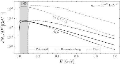
Figure 2: The differential axion spectra integrated over the first 10 s after the SN for our fiducial SN1987A simulation SFHo-18.6 Bollig et al. (2020), corresponding to the formation of a 1.553 $M_{\odot}$ NS. We separate the spectra into contributions from the Primakoff production, bremsstrahlung from nucleons, and processes involving pions. The ALP curves assume no UV contributions to the axion-quark couplings, with the couplings generated in the IR under the RG flow, while the curve labeled ‘QCD KSVZ’ uses the relations $C_{ann}/C_{a\gamma\gamma}\simeq 0.01$, $C_{app}/C_{a\gamma\gamma}\simeq 0.24$ and $C_{a\pi N}/C_{a\gamma\gamma}\simeq 0.13$ appropriate for a KSVZ-type QCD axion.

axion spectra $dN_{a}/dE$ integrated over the 10 s simulation (our fiducial model) for two different theory assumptions for the axion. Both cases have $g_{a\gamma\gamma}=10^{-12}$ GeV^-1, but that labeled ‘ALP’ has no tree-level coupling to quarks and only the loop-induced couplings described previously. The second case, labeled ‘QCD KSVZ’, has $C_{ann}/C_{a\gamma\gamma}\simeq 0.01$, $C_{app}/C_{a\gamma\gamma}\simeq 0.24$ and $C_{a\pi N}/C_{a\gamma\gamma}\simeq 0.13$, which are the ratios expected in the KSVZ QCD axion model. (See also the ‘light’ QCD axion models proposed in Hook (2018); Di Luzio et al. (2021).) For each scenario we show the contributions to the luminosity from Primakoff production, nucleon bremsstrahlung involving nucleons only, and processes involving pions. Interestingly, even in the axion-like particle scenario with no tree-level fermion couplings the contribution to the luminosity from hadrons dominates the Primakoff production. We also indicate the energy range of the SMM telescope that observed SN1987A; the majority of the pion-induced emission is outside of SMM’s energy range.

Axion-photon conversion.— We consider, for the first time, the conversion of axions-to-photons on the stellar magnetic fields surrounding the progenitor star for the SN. First, it is instructive to make a rough estimate of the Galactic versus stellar conversion probabilities, with the low-axion-mass approximation $P_{a\to\gamma}\sim g_{a\gamma\gamma}^{2}B^{2}L^{2}$, with $B$ the astrophysical magnetic field strength and $L$ the length of the magnetic field domain. Typical values for Galactic magnetic fields are $B\sim\mu$G and $L\sim 1$ kpc, yielding $P_{a\to\gamma}\sim 10^{-5}(g_{a\gamma\gamma}/10^{-12}\,\,{\rm GeV})^{2}$. On the other hand, the progenitor of the SN1987A was a blue supergiant (BSG), with a surface magnetic field strength $B_{0}\sim{\rm kG}$ Orlando et al. (2019) and a radius $r_{0}\approx 45\pm 15$ $R_{\odot}$ Woosley (1988). (We fix $r_{0}=45$ $R_{\odot}$ as this is a subdominant source of uncertainty relative to the surface magnetic field strength.) Given that $\mu{\rm G}\times{\rm kpc}\sim{\rm kG}\times(45R_{\odot})$, we estimate that the axion-to-photon conversion probability on the stellar magnetic fields should be comparable to that on the Galactic fields. On the other hand, the estimates above are only valid in the low mass limit; in particular, they are valid when $m_{a}^{2}/(2E)\times L\ll 1$, where $E$ is the energy of the axion. Taking $E\sim 100$ MeV, we thus estimate that the axion-conversion probability becomes degraded for $m_{a}\gtrsim 2\times 10^{-11}$ eV ($m_{a}\gtrsim 5\times 10^{-5}$ eV) for conversion on the Galactic (stellar) magnetic fields.

Core-collapse supernova form PNS when the collapsing core reaches nuclear densities; the formation of the PNS causes the in-falling matter to bounce outwards, forming a rapidly expanding shock-wave that blows apart the star. The outward propagating shock-wave travels slower than the speed of light. In contrast, the axions propagate outwards faster, nearly at the speed of light. Thus, the axions leave the star well ahead of the shock-wave. They encounter the still-pristine magnetic fields of the progenitor star because the change in the magnetic field induced by the bounce propagates relatively slowly out from the stellar core at the Alfvén velocity (see, e.g., Suzuki et al. (2008)).

There was no direct measurement of the magnetic field strength of the SN1987A precursor star Sk -69 202, but there are indirect hints from radio and X-ray data in the decades following the SN that the precursor star had a surface field strength $B_{0}\sim 3$ kG Orlando et al. (2019). This field strength is in line with the $\sim$kG level magnetic field strengths expected for BSGs Petermann et al. (2015), especially considering that Sk -69 202 likely formed from a merger of two smaller stars Sana et al. (2012); Morris and Podsiadlowski (2007). BSGs like Sk -69 202 have surface field strengths in the range $\sim$100 G to 10 kG Donati and Landstreet (2009), and below we use this range of field strengths when bracketing the uncertainties in the axion-induced gamma-ray signal.

We model the magnetic field of the progenitor star as a dipole field, in which case $B$ falls as $1/r^{3}$ away from the stellar surface. On the other hand, we note that this is a conservative choice, as the rotation of the progenitor star and its stellar wind may have led to a Parker Spiral type field Parker (1958); Orlando et al. (2019), as in the case of the Sun, for which $B$ falls more slowly, with $1/r$ and $1/r^{2}$ components, away from the surface. We assume for simplicity that the axions travel radially outwards at the mid-plane, such that at every point exterior to the star the magnetic field is perpendicular to the axion trajectory. The axion-photon mixing equations are described in detail in the SM, including the non-linear Euler-Heisenberg (EH) term in the effective Lagrangian for electromagnetism (see, e.g., Safdi (2022)), which reduces the conversion probabilities given the large axion energies and high field strengths. Note that we neglect the effects of the photon plasma frequency in the medium exterior to the star, since for this to be important the free electron density would need to exceed $n_{e}\sim 10^{10}$ cm^-3, which is not expected.

SMM data analysis from SN1987A.— We compute the mass-dependent upper limits on $g_{a\gamma\gamma}$ from the non-observation of excess gamma-rays from SN1987A with the SMM. We use the SMM data and instrument response approximations presented in Hoof and Schulz (2023). (See the SM.) We find no evidence for axions, consistent with previous works, with the 95% upper limits illustrated in Fig. 1. The limit shaded in blue labeled ‘ALP SN1987A’ accounts for the conversion in the Galactic magnetic field (low masses), with the fields modeled using the updated Galactic model Unger and Farrar (2023), and for axion-to-photon conversion in the stellar magnetic field of the progenitor (dominating the sensitivity for $m_{a}$ above $\sim$$10^{-9}$ eV). We account for Primakoff production and hadronic processes, with our fiducial loop-level couplings to hadrons. Only accounting for Primakoff emission weakens the limit at low $m_{a}$ from $|g_{a\gamma\gamma}|\lesssim 2.4\times 10^{-12}$ GeV^-1 to $|g_{a\gamma\gamma}|\lesssim 4\times 10^{-12}$ GeV^-1. On the other hand, changing to the older Galactic magnetic field model in Ref. Jansson and Farrar (2012), matching that used in previous works Payez et al. (2015); Hoof and Schulz (2023), weakens the low-mass axion limit to $|g_{a\gamma\gamma}|\lesssim 3.2\times 10^{-12}$ GeV^-1. Using the magnetic field model in Jansson and Farrar (2012) and only accounting for Primakoff emission, as in Refs. Payez et al. (2015); Hoof and Schulz (2023), we find a nearly identical upper limit to that in Hoof and Schulz (2023) at $m_{a}=0$ eV ($<$ 10% difference), suggesting that the differences in SN simulations are sub-leading.

Our upper limits in Fig. 1 take a stellar surface field strength of 100 G to be conservative, even though higher field strengths are favored. Our axion-like particle limit (labeled ‘ALP SN1987A’) excludes new parameter space for $m_{a}\gtrsim 10$ $\mu$eV. The upper limit labeled ‘KSVZ-like axion SN1987A’ assumes that the ratios of $C_{app}/C_{a\gamma\gamma}$, $C_{ann}/C_{a\gamma\gamma}$, and $C_{a\pi N}/C_{a\gamma\gamma}$ are as expected in the KSVZ QCD axion model. This upper limit is around an order of magnitude away in terms of $g_{a\gamma\gamma}$ from probing the KSVZ QCD axion model for $m_{a}\gtrsim 10^{-4}$ eV, strongly motivating future observations with increased sensitivity.

Our axion-like particle upper limit in Fig. 1 excludes much of the parameter space that will be probed by the ALPS II light-shining-through-walls experiment Bähre et al. (2013); Oceano (2024); Ringwald (2024); taking a more realistic but less conservative surface magnetic fields strength of $B_{0}=1$ kG, we exclude the full parameter space to be probed by ALPS II (see the SM).

Note that our results are strictly speaking only valid for, roughly, $|g_{a\gamma\gamma}|\lesssim 10^{-8}$ GeV^-1 ($m_{a}\lesssim 10^{-2}$ eV) for the axion-like particle model (the KSVZ QCD axion), as for larger couplings we estimate that the axion luminosity 1 s post-bounce exceeds the neutrino luminosity. The axion model at larger couplings is disfavored Raffelt (1996); Caputo and Raffelt (2024), and modeling this scenario would require including the back-reaction of the axion emission in the SN simulations.

GALAXIS: Galactic Axion Instrument for Supernova.— If a Galactic SN went off today, we estimate that the chance Fermi-LAT would be looking at the correct place at the correct time to catch the $\sim$10 s axion-induced burst is only around $\sim$20%, accounting for the finite FOV of the instrument and down-time during its orbit. On the other hand, if the next SN went off directly above Fermi (at its zenith), the estimated 95% upper limits on $g_{a\gamma\gamma}$ we would be able to obtain are illustrated in Fig. 1. We use the Fermitools to obtain the instrument response with the P8R3_TRANSIENT020_V2 event class; we estimate $\sim$0 background events over the $\sim$10 s duration of the SN. The effective area at zenith at $E=200$ MeV is $\sim$$0.72$ m². We illustrate the expected 95% upper limits under the null hypothesis for the axion-like particle scenario, the KSVZ-like axion, and a DFSZ-like scenario, scanning over $\tan\beta$. (We show the strongest and weakest limits across the range of $\tan\beta$; see the SM for details.) We make these projections using our fiducial SFHo-18.6 SN simulation, and we assume a distance of 10 kpc to the next Galactic SN. We only account for axion-photon conversion on the stellar magnetic fields of the progenitor star, assuming a 1 kG surface magnetic field for a BSG SN that is otherwise the same as SN1987A. (The axions could also convert to photons on the Galactic magnetic field, enhancing the low-mass sensitivity.) In the SM we discusses red supergiant (RSG) SN, which are more prevalent and as we show have comparable sensitivity.

Without new instrumentation the opportunity to probe QCD axions using gamma-ray observations of the next Galactic SN will almost certainly be lost, since the event will likely have no advanced warning (but see Ge et al. (2020)) and not be within the FOV of the Fermi-LAT. The proposed Advanced Particle-astrophysics Telescope (APT) Alnussirat et al. (2021); Buckley et al. (2021) may have an increased FOV relative to the Fermi-LAT, though it will likely also not be $4\pi$. We thus propose a full-sky gamma-ray telescope network, which we call the GALactic AXion Instrument for Supernova (GALAXIS) (see Fig. 3).

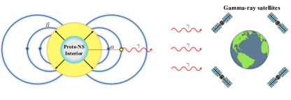
Figure 3: The GALAXIS gamma-ray satellite constellation proposed in this work to search for axion-induced gamma-ray signatures from core-collapse SN and NS-NS mergers. The axions are generated in the hot PNS cores and then convert to gamma-rays on the stellar magnetic fields of the progenitor stars. Such an instrument with a Fermi-LAT-level effective area could potentially probe QCD axions for any $m_{a}\gtrsim 50$ $\mu$eV, depending on the properties of the event.

The idea behind GALAXIS is to establish a full-sky constellation of gamma-ray satellites to provide continuous $4\pi$ coverage of the gamma-ray sky between $\sim$100 MeV and $\sim$1 GeV. (See also the recent work Lella et al. (2024b) that made a related proposal.) The network would consist of multiple (e.g., $\sim$5 or more) gamma-ray telescopes on different orbital trajectories, such that any future SN would be in view of at least one telescope in the network. Such an instrument would complement the multiple gamma-ray telescope constellations in planning stages at energies below $\sim$10 MeV (see Bloser et al. (2022) and references therein). We leave a full technical investigation to future work. In Fig. 1 we simply assume for the projections that the GALAXIS instrument response is identical to that of the on-axis Fermi-LAT (see the SM). The main improvements with the future projections relative to the SN1987A constraints come from the distance to the SN, the large effective area and improved background rate of GALAXIS (i.e., Fermi-LAT) relative to the SMM, and the inclusion of higher-energy photons above $\sim$100 MeV that allow for probing pion-induced axions. GALAXIS may reach sensitivity to the QCD axion, making it competitive with upcoming efforts to target QCD axions such as IAXO Armengaud et al. (2019), MADMAX Beurthey et al. (2020), and ALPHA Millar et al. (2022).

Discussion.— In this Letter we focus on axion-induced gamma-ray signals from nearby PNS formed after core-collapse SN due to axion-photon conversion in the stellar magnetic fields of the progenitor stars. However, there are a number of related axion-induced gamma-ray signals that may proceed similarly and be detectable with the proposed GALAXIS gamma-ray observatory. For example, in cases where the compact remnant of the core-collapse SN is a black hole (as suggested could be the case for SN1987A in Bar et al. (2020), though this is now disfavored Page et al. (2020); Fransson et al. (2024)), a hot, massive PNS remnant forms prior to collapse. It would be interesting to study the axion-induced gamma-ray signal from such a short-lived remnant with dedicated simulations. Similarly, NS-NS mergers can lead to stable NSs or hypermassive remnants that collapse to black holes; in either case, exceedingly hot PNSs form within the first tens of ms, with temperatures that can exceed those in core-collapse SN. As we show in the SM, nearby NS-NS mergers (within $\sim$50 Mpc of Earth) are promising targets for gamma-ray axion searches. (See also Dietrich and Clough (2019); Harris et al. (2020); Dev et al. (2024).) Given the compact sizes of the NSs, these objects can potentially probe higher axion masses and may even reach QCD axion sensitivity near $\sim$1 meV (see the SM). NS-NS mergers, along with SN within the local group and nearby galaxy clusters, can be expected on a near yearly basis, meaning that the proposed GALAXIS instrument would have frequent opportunities for axion science.

Supplementary Material for Supernova axions convert to gamma-rays in magnetic fields of progenitor stars
Claudio Andrea Manzari, Yujin Park, Benjamin R. Safdi, and Inbar Savoray

[sections]

I Axion Emission from Supernovae

Axions are produced in hot PNSs through the diagrams illustrated in Fig. S1. Here, we provide formulae for their emissivities, summarizing the results of Refs. Raffelt (1986); Carenza et al. (2019); Ho et al. (2023). Note that we account for the effects of degenerate media and gravitational redshift Buschmann et al. (2021); Caputo et al. (2022).

Figure S1: Diagrams contributing to axion production within a hot PNS from (left to right) Primakoff production, nucleon bremsstrahlung, pion-axion conversion, and pion-axion conversion with virtual nucleon or $\Delta$ exchange. Diagrams related to these by symmetry are suppressed.

I.a Primakoff

The two-photon coupling of the axion,

$$\mathcal{L}\supset\frac{1}{4}g_{a\gamma\gamma}F_{\mu\nu}\tilde{F}^{\mu\nu}a=g_{a\gamma\gamma}\,\mathbf{E}\cdot\mathbf{B}\;a\,,$$ (S1)

allows for axion-to-photon conversion in the electric field of a spectator charged particle, as shown in Fig. S2.

Figure S2: Primakoff conversion of a photon into an axion in the electric field of a particle with charge $Ze$.

The axion production rate per unit energy is

$$\frac{d\dot{N}_{a}}{d\omega}=4\pi\int dRR^{2}\frac{d\dot{n}_{a}}{d\omega}\,,$$ (S2)

where the integral is over the radial direction in the PNS. We define $\Gamma_{\gamma}(\omega)$ to be the Primakoff conversion rate, so that

$$\frac{d\dot{n}_{a}}{d\omega}=\frac{\omega^{2}(1-\omega_{p}^{2}/\omega^{2})}{\pi^{2}}\frac{1}{e^{\omega/T}-1}\Gamma_{\gamma}(\omega)\,,$$ (S3)

with $\omega_{p}$ the photon plasma frequency. Ignoring recoil effects one finds

$$\Gamma_{\gamma}(\omega)=\frac{g_{a\gamma\gamma}^{2}Z^{2}\,\alpha\,n^{\rm eff}}{8\pi}\int d\Omega\frac{|\mathbf{k}_{\gamma}\times\mathbf{k}_{a}|^{2}}{|\mathbf{q}|^{2}(|\mathbf{q}|^{2}+\kappa^{2})}\,,$$ (S4)

where $n^{\rm eff}$ is the effective number density of the target, $Z$ is the atomic number of the target, $\mathbf{k}_{\gamma}$ and $\mathbf{k}_{a}$ are the momenta of the incoming photon and outgoing axion, and $\mathbf{q}=\mathbf{k}_{\gamma}-\mathbf{k}_{a}$ is the momentum transfer. Following Ref. Raffelt (1986) we accounted for the plasma screening effect through the Debye factor $\kappa$. Expanding the momenta in (S4) up to $\mathcal{O}(\omega_{p}^{2}/\omega^{2},m_{a}^{2}/\omega^{2})$, we find

$$\Gamma_{\gamma}(\omega)=\frac{g_{a\gamma\gamma}^{2}Z^{2}\,\alpha n^{\rm eff}(1-\xi)}{4\omega^{2}(2-\xi)^{3}}\bigg{[}-2\omega^{2}(2-\xi)+(\kappa^{2}+2(2-\xi)\omega^{2})\log\bigg{(}\frac{\kappa^{2}+2\omega^{2}(2-\xi)}{\kappa^{2}}\bigg{)}\bigg{]}\,,$$ (S5)

where $\xi=\frac{\omega_{p}^{2}+m_{a}^{2}}{\omega^{2}}$.

The Primakoff process is most relevant when the spectator particle is non-relativistic. In a PNS, the most important targets are thus protons. The protons are partially degenerate and their effective number density is given by Payez et al. (2015)

$$n_{p}^{\rm eff}=2\int\frac{d^{3}p}{(2\pi)^{3}}f_{p}(1-f_{p})\,,$$ (S6)

where $f_{p}$ is the Fermi-Dirac distribution function for the proton. Here we also note that there are finite temperature and density effects in a PNS that reduce the proton mass, enhancing its degeneracy. These effects are taken into account in our results. The Debye scale for the proton Coulomb potential is controlled by the longitudinal component of the polarization tensor Raffelt (1986). Using the one-loop, non-relativistic approximation for the polarization tensor gives Payez et al. (2015)

$$\kappa^{2}\simeq\frac{4\alpha m_{p}^{*}}{\pi}\int dp\,f_{p}=\frac{4\pi\alpha n_{p}^{\rm eff}}{T}\,,$$ (S7)

where $m_{p}^{*}$ is the effective proton mass. Finally, the plasma frequency in a degenerate medium as in a PNS is given by

$$\omega_{p}^{2}=\frac{4\pi\alpha n_{e}}{E_{F}}=\frac{4\alpha}{3\pi}p_{F}^{2}v_{F}\,,$$ (S8)

where $n_{e}$ is the electron number density and $E_{F},\,p_{F},\,v_{F}$ are the Fermi energy, momentum and velocity, respectively. Note that $v_{F}\approx 1$ for the electron.

I.b Nucleon-Nucleon Bremsstrahlung

A relevant process of axion production in a PNS is the nucleon-nucleon (NN) axion bremsstrahlung, which involves the axion-nucleon coupling. In this work we follow Ref. Carenza et al. (2019), modelling this process including the effect of a massive pion propagator, the contribution of the $\rho$-meson exchange to mimic the effects of two-pion exchange, the medium modification of the nucleon mass, and accounting for nucleon multiple scatterings.

Figure S3: Nucleon-Nucleon Bremsstrahlung production of an axion.

With the axion-nucleon interaction defined as

$${\mathcal{L}}\supset\frac{C_{aNN}}{2f_{a}}\partial_{\mu}a\bar{N}\gamma^{\mu}\gamma^{5}N\,,$$ (S9)

the axion production rate per unit energy is

$$\frac{d\dot{n}_{a}}{d\omega}=\frac{\omega\,\Gamma_{\sigma}}{16\pi^{2}}\frac{n_{B}}{f_{a}^{2}}\,\bigg{[}s^{nn}(\omega/T)+s^{pp}(\omega/T)+s^{np}(\omega/T)\bigg{]}\,,$$ (S10)

where $\Gamma_{\sigma}$ is the nucleon “spin fluctuation rate” and $s^{nn}(\omega/T)$, $s^{pp}(\omega/T)$ and $s^{np}(\omega/T)$ are 5-dimensional integrals, depending of the coefficients $C_{app}$ and $C_{ann}$, that can be found in Ref. Carenza et al. (2019).

I.c Pion-Axion Conversion

The Feynman diagrams for pion conversion are shown in Fig. S4.

Figure S4: Axion-pion conversion processes in a SN through a contact interaction or the exchange of a virtual nucleon or $\Delta$ baryon.

The axion emission rate per unit energy is Ho et al. (2023); Carenza (2023)

$$\begin{split}\frac{d\dot{n}_{a}}{d\omega}=&\mathcal{C}_{a}^{p\pi^{-}}\,\frac{(m_{N}T)^{3/2}}{2^{3/2}\pi^{5}f_{a}^{2}}\left(\frac{m_{N}}{2f_{\pi}}\right)^{2}\left(\omega^{2}-m_{a}^{2}\right)^{\frac{3}{2}}\,\frac{\Theta(\omega-\max\left(m_{a},m_{\pi}\right))}{\exp{\left(x_{a}-y_{\pi}-\hat{\mu}_{\pi}\right)}-1}\,\frac{(\omega^{2}-m_{\pi}^{2})^{\frac{1}{2}}}{\omega^{2}+\Gamma_{\sigma}^{2}/4}\\ &\times\int_{0}^{\infty}du\,u^{2}\frac{1}{\exp{\left(u^{2}-\hat{\mu}_{p}\right)}+1}\frac{1}{\exp{\left(-u^{2}+\hat{\mu}_{n}\right)}+1}\,,\end{split}$$ (S11)

where $y_{\pi}=m_{\pi}/T$, $\hat{\mu}$ is the degeneracy parameter for pions and nucleons, and the Heaviside theta function fixes the minimal threshold energy. The coefficient $\mathcal{C}_{a}^{p\pi^{-}}$, at first order in $1/m_{N}$, is given by Ho et al. (2023)

$$\begin{split}\mathcal{C}_{a}^{p\pi^{-}}&=\frac{2g_{A}^{2}\big{(}2C_{+}^{2}+C_{-}^{2}\big{)}}{3}\bigg{(}\frac{\sqrt{\omega^{2}-m_{\pi}^{2}}}{m_{N}}\bigg{)}^{2}+C_{a\pi N}^{2}\bigg{(}\frac{\omega}{m_{N}}\bigg{)}^{2}+\frac{g_{A}^{2}C_{aN\Delta}^{2}}{9}\mathcal{F}_{a\pi N}\bigg{(}\frac{\sqrt{\omega^{2}-m_{\pi}^{2}}}{m_{N}}\bigg{)}^{2}\\ &\quad-\frac{4\sqrt{3}g_{A}^{2}C_{aN\Delta}}{9}\mathcal{F}_{aN\Delta}\bigg{(}\frac{\sqrt{\omega^{2}-m_{\pi}^{2}}}{m_{N}}\bigg{)}^{2}\,,\end{split}$$ (S12)

with

$$\begin{split}\mathcal{D}&=\big{[}\big{(}\Delta m-E_{\pi}\big{)}^{2}+\Gamma_{\Delta}^{2}/4\big{]}\big{[}\big{(}\Delta m+E_{\pi}\big{)}^{2}+\Gamma_{\Delta}^{2}/4\big{]}\,,\quad\mathcal{F}_{a\pi N}=\mathcal{D}^{-1}E_{\pi}^{2}\Big{(}\Delta m^{2}+2E_{\pi}^{2}+\frac{\Gamma_{\Delta}^{2}}{4}\Big{)}\,,\\ \mathcal{F}_{aN\Delta}&=\mathcal{D}^{-1}E_{\pi}\Big{[}\big{(}\Delta m^{2}-E_{\pi}^{2}\big{)}\big{(}C_{+}\Delta m+C_{-}E_{\pi}\big{)}+\frac{\Gamma_{\Delta}^{2}}{4}\big{(}C_{+}\Delta m-C_{-}E_{\pi}\big{)}\Big{]}\,,\end{split}$$ (S13)

where $C_{+}=C_{app}+C_{ann}$, $C_{-}=C_{ann}-C_{app}$, $\Gamma_{\Delta}=117$ MeV is the width of the $\Delta$-resonance, $\Delta m=m_{\Delta}-m_{N}^{*}$ and $g_{A}\simeq 1.28$ is the axial-vector coupling constant. The axion-nucleon-pion and axion-nucleon-$\Delta$ couplings are defined in the next section.

Note that referring to e.g. Fig. 2 the pion-conversion processes give non-trivial emission up to high energies $\sim$1 GeV. On the other hand, the heavy baryon chiral EFT is not expected to be valid for axion energies of order the nucleon mass (around 1 GeV). With that said, we stress that due to the steeply falling spectral shape with energy, the axions with energies around 1 GeV make a negligable contribution to our final result. For example, only including axion energies less than 500 MeV changes our projected upper limits by less than 1%. Additionally, we note that in some regions of the PNS our simulations predict a pion condensate ($\mu_{\pi^{-}}>m_{\pi^{-}}$). In this work we do not attempt to correctly describe this phase or to account for nucleon-pion interactions that can affect the number density Carenza et al. (2021). On the other hand, we verify that removing the small regions that give pion condensates leads to an imperceptible change in our final results. Still, it is the pion condensate that gives rise to the sharp spectral features seen in e.g. Fig. S13.

II Axion-matter couplings under RG flow

In this section we consider axion-like particle scenarios where in the UV the axion only couples to electroweak gauge bosons. As is well established Srednicki (1985); Bauer et al. (2017), the axion-matter couplings are generated under the RG flow. We review the expected loop-induced couplings here.

By assumption, in the UV the axion only couples to the Standard Model through the terms

$$\mathcal{L}\supset-\frac{1}{4}C_{aWW}\frac{g_{2}^{2}}{8\pi^{2}f_{a}}a\,W_{\mu\nu}^{a}\tilde{W}^{a\,\mu\nu}-\frac{1}{4}C_{aBB}\frac{g_{1}^{2}}{8\pi^{2}f_{a}}a\,B_{\mu\nu}\tilde{B}^{\mu\nu}\,,$$ (S14)

with $W_{\mu\nu}$ and $B_{\mu\nu}$ the $SU(2)_{L}$ and $U(1)_{Y}$ field strengths, respectively, and where by assumption we do not allow the axion-like particle to couple to QCD. Note that the coupling constants $g_{1}$ and $g_{2}$ are not topological quantities and therefore are not scale invariant, while $C_{aWW}$ and $C_{aBB}$ do not evolve under RG flow. At the electroweak symmetry breaking scale, we integrate out the heavy fields, and we are left with the effective Lagrangian

$$\mathcal{L}\supset-\frac{1}{4}C_{a\gamma\gamma}\frac{e^{2}}{8\pi^{2}f_{a}}a\,F_{\mu\nu}\tilde{F}^{\mu\nu}\,,$$ (S15)

where $F_{\mu\nu}$ is the electromagnetic field tensor and the matching simply reads $C_{a\gamma\gamma}=C_{aWW}+C_{aBB}$.

II.a Couplings with Nucleons

On the other hand, the couplings of an axion to fermions are not topological and are induced through RG running. Recall that the coefficient $C_{aqq}$ describing the axion coupling to quark fields $q$ is defined by

$$\mathcal{L}\supset\frac{C_{aqq}}{2f_{a}}\partial^{\mu}a\,\bar{q}\gamma_{\mu}\gamma_{5}\,q\,.$$ (S16)

Then, at one-loop we have (see, e.g., Bauer et al. (2021))

$$\frac{dC_{aqq}(\mu)}{d\ln{\mu}}=-\frac{3}{128\pi^{4}}\left(\frac{3}{4}g_{2}^{4}C_{aWW}+(\mathcal{Y}_{Q}^{2}+\mathcal{Y}_{q}^{2})g_{1}^{4}C_{aBB}\right)\,.$$ (S17)

where $\mathcal{Y}_{Q}$ and $\mathcal{Y}_{q}$ are the hypercharges of the left-handed quark doublet and right-handed singlet, respectively.
Including the one-loop RG flow for the gauge coupling

$$\frac{dg_{1}}{d\ln\mu}=\frac{41}{6}\frac{g_{1}^{3}}{16\pi^{2}}\,,\qquad\frac{dg_{2}}{d\ln\mu}=-\frac{19}{6}\frac{g_{2}^{3}}{16\pi^{2}}\,,$$ (S18)

we obtain

$$C_{aqq}(\mu)=\frac{3}{128\pi^{4}}\ln\left(\frac{\Lambda}{\mu}\right)\bigg{(}\frac{3}{4}C_{aWW}g_{2}(\Lambda)^{2}g_{2}(\mu)^{2}+(\mathcal{Y}_{Q}^{2}+\mathcal{Y}_{q}^{2})C_{aBB}g_{1}(\Lambda)^{2}g_{1}(\mu)^{2}\bigg{)}\,,$$ (S19)

with $\Lambda\sim 4\pi f_{a}$ the UV scale where, by construction, $C_{q}(\Lambda)=0$. From (S19) we can compute $C_{q}(\mu=m_{z})$ at the EW scale, given by the $Z$-boson mass $m_{z}$. Below the electroweak scale the RG evolution proceeds only through the contribution of $U(1)_{\rm EM}$:

$$\frac{dC_{aqq}(\mu)}{d\ln{\mu}}=-\frac{3}{64\pi^{4}}Q^{2}e^{4}C_{a\gamma\gamma}\,,$$ (S20)

with $Q$ the electromagnetic charge of the quark. (Note that we neglect the running of the fine structure constant as we expect this contribution to be subdominant.) In the IR, at $\Lambda_{\rm QCD}<\mu<m_{z}$, we thus find

$$C_{aqq}(\mu)=C_{aqq}(m_{Z})+\frac{3}{64\pi^{4}}\ln\left(\frac{m_{Z}}{\mu}\right)Q^{2}e^{2}(m_{Z})e^{2}(\Lambda_{\rm QCD})C_{a\gamma\gamma}\,.$$ (S21)

Following Ref. Grilli di Cortona et al. (2016), we extract the couplings of an axion to nucleons matching onto an effective Lagrangian valid at energies much lower than the QCD mass gaps $\sim\mathcal{O}(100\,\rm{MeV})$. The matching scale is conveniently chosen to be $\sim 2$ GeV, and we obtain

$${\cal L}_{N}=\bar{N}v^{\mu}D_{\mu}N+\frac{\partial_{\mu}a}{f_{a}}\Bigl{\{} \frac{C_{auu}-C_{add}}{2}(\Delta u-\Delta d)\bar{N}\frac{\gamma^{\mu}\gamma^{5}}{2}\sigma^{3}N$$

$$+\Bigl{[}\frac{C_{auu}+C_{add}}{2}(\Delta u+\Delta d)+\sum_{q=s,c,b,t}C_{aqq}\Delta q\Bigr{]}\bar{N}\frac{\gamma^{\mu}\gamma^{5}}{2}N\Bigr{\}}\,,$$ (S22)

where $C_{aqq}=C_{aqq}(\mu=2\,\rm{GeV})$ and $N=(p,\,n)$. From low energy experiments and lattice determinations the matrix elements read Grilli di Cortona et al. (2016)

$$\Delta u(2\,{\rm{GeV}})=0.897(27),\quad\Delta d(2\,{\rm{GeV}})=-0.376(27),\quad\Delta s(2\,{\rm{GeV}})=-0.026(4)\,,$$ (S23)

and the contribution from heavier quarks can be safely neglected. In analogy with (S16), the interaction terms can be rewritten as

$${\mathcal{L}}\supset\frac{\partial_{\mu}a}{2f_{a}}\Bigl{[}C_{app}\bar{p}\gamma^{\mu}\gamma^{5}p+C_{ann}\bar{n}\gamma^{\mu}\gamma^{5}n\Bigr{]}\,,$$ (S24)

with

$$\begin{split}&C_{app}=0.88(3)C_{u}-0.39(2)C_{d}-0.038(5)C_{s}\,,\\ &C_{ann}=0.88(3)C_{d}-0.39(2)C_{u}-0.038(5)C_{s}\,.\end{split}$$ (S25)

Note that we neglect the self-renormalization of the fermionic axial current, which is sub-leading to the effect induced by the photon coupling, since we assume $C_{aqq}(\Lambda)=0$ in the UV.

II.b Axion-Nucleon-Pion and Axion-Nucleon-$\Delta$ Couplings

The axion-pion-nucleon coupling can be described in heavy baryon chiral perturbation theory Chang and Choi (1993); Vonk et al. (2021) and reads

$$\mathcal{L}_{a\pi N}=i\frac{\partial_{\mu}a}{2f_{a}}C_{a\pi N}(\pi^{+}\bar{p}\gamma^{\mu}n-\pi^{-}\bar{n}\gamma^{\mu}p)\,,$$ (S26)

with $C_{a\pi N}=(C_{app}-C_{ann})/{\sqrt{2}g_{A}}$. Similarly, one can compute the axion-nucleon-$\Delta$ interaction Ho et al. (2023) as

$$\mathcal{L}_{aN\Delta}=i\frac{\partial_{\mu a}}{2f_{a}}C_{aN\Delta}\bigg{[}\bar{p}\,\Delta^{\mu\,+}+\bar{\Delta}^{\mu\,+}\,p+\bar{n}\,\Delta^{\mu\,0}+\bar{\Delta}^{\mu\,0}\,n\bigg{]}\,,$$ (S27)

where $C_{aN\Delta}=-\sqrt{3}(C_{app}-C_{ann})/2$.

II.c Numerical Results

Taking the UV scale to be $\Lambda=10^{9}\,{\rm GeV}$, then (S21) together with (S25) gives

$$\begin{split}&C_{app}\sim 3.5\times 10^{-5}\,C_{aBB}+2.1\times 10^{-4}\,C_{aWW}\,,\\ &C_{ann}\sim-5.6\times 10^{-6}\,C_{aBB}+2.1\times 10^{-4}\,C_{aWW}\,.\end{split}$$ (S28)

For a generic UV completion where $C_{aWW}\sim C_{aBB}$, we thus expect $C_{app}/C_{a\gamma\gamma}\sim C_{ann}/C_{a\gamma\gamma}\sim 10^{-4}$, $C_{a\pi N}/C_{a\gamma\gamma}\sim 10^{-5}$, and $C_{aN\Delta}/C_{a\gamma\gamma}\sim 2\times 10^{-5}$, justifying the benchmark values assumed for an axion-like particle model in the main Letter.

III KSVZ and DFSZ Benchmarks

Throughout this Letter, we show our exclusion limits and projections for the KSVZ and DFSZ axion benchmarks. Here, we briefly summarize the coupling strengths expected for these models (see, e.g., Di Luzio et al. (2020) for a more complete review).

Recall that in the KSVZ axion model, the Standard Model is extended by a complex scalar and a vector-like fermion that interact through a Yukawa interaction. The scalar is a singlet under the SM gauge groups while the fermion is in the fundamental representation of $SU(3)_{C}$. Both fields are charged under a global $U(1)_{\rm PQ}$ symmetry. In this minimal setup, the axion-photon coupling originates purely from axion-pion mixing in the IR, while the couplings of the axion to nucleons arise from the axion coupling to gluons. The couplings of the axion to the photon, neutron and proton are Grilli di Cortona et al. (2016):

$$C_{a\gamma\gamma}\approx-1.92\,,\quad C_{ann}\approx-0.02\,,\quad C_{app}\approx-0.47\,.$$ (S29)

Conversely, in the DFSZ setup, the Standard Model quark fields are charged under $U(1)_{PQ}$ and the scalar content of the SM has to be extended by one singlet and at least one additional Higgs doublet. The axion-photon coupling is therefore modified by the presence of an electromagnetic anomaly, and the couplings to quarks have a tree-level contribution. For the extensions with a single additional Higgs doublet, the couplings to the photon, neutron and proton are

$$C_{a\gamma\gamma}\approx 0.75\,,\quad C_{ann}\approx(-0.617+0.435\sin^{2}\beta)\,,\quad C_{app}\approx(0.254-0.414\sin^{2}\beta)\,,$$ (S30)

where $\tan\beta$ is the ratio between the vacuum expectation values of the two Higgs doublets in the theory. In this work, we present limits for the DFSZ scenario as a band obtained varying the value of $\tan{\beta}$ (see, e.g., Fig. 1).

IV Magnetic field modeling and axion-photon conversion

Here, we briefly summarize how we compute the axion-to-photon conversion probabilities. Assuming the axion and photon wavelengths are much smaller than the propagation length, the second-order axion-photon mixing equations can be linearized to first-order mixing equations Raffelt and Stodolsky (1988). Hence, the equation of motion for a mode of energy $\omega$ that propagates in the z-direction through an external magnetic field $\mathbf{B}(\mathbf{x})$, in a plasma with electron density $n_{e}(\mathbf{x})$, reads

$$\bigg{(}(\omega-i\partial_{z})\mathbb{I}+M(z)\bigg{)}\begin{pmatrix}|\gamma_{\perp}(z)\rangle\\ |\gamma_{\parallel}(z)\rangle\\ |a(z)\rangle\\ \end{pmatrix}=0\,,$$ (S31)

where $|\gamma_{\parallel(\perp)}\rangle$ represents an electromagnetic wave with the electric field oscillating in the direction parallel (perpendicular) to the projection of $\mathbf{B}(\mathbf{x})$ on the $x-y$ plane $\mathbf{B}_{T}$, and

$$M(z)=\begin{pmatrix}-\frac{\omega_{p}^{2}(\mathbf{x})}{2\omega}+\delta^{\perp}_{\rm HE}(\mathbf{x})&0&0\\ 0&-\frac{\omega_{p}^{2}(\mathbf{x})}{2\omega}+\delta^{\parallel}_{\rm HE}(\mathbf{x})&g_{a\gamma\gamma}\frac{B_{T}(\mathbf{x})}{2}\\ 0&g_{a\gamma\gamma}\frac{B_{T}(\mathbf{x})}{2}&-\frac{m_{a}^{2}}{2\omega}\\ \end{pmatrix}\,.$$ (S32)

Here, $\omega_{p}(\mathbf{x})=\sqrt{4\pi e^{2}n_{e}(\mathbf{x})/m_{e}}$ is the plasma frequency for a non-degenerate medium (e.g., the electron interstellar plasma or the exterior plasma of a star), and the Euler-Heisenberg term, $\delta^{\parallel}_{\rm HE}(\mathbf{x})=7\alpha_{\rm em}\omega/(90\pi B_{\rm crit}^{2})|\mathbf{B}(\mathbf{x})\times\hat{z}|^{2}\,,\delta^{\perp}_{\rm HE}(\mathbf{x})=4/7\delta^{\parallel}_{\rm HE}(\mathbf{x})$  with $B_{\rm crit}=4.41\times 10^{13}$ G, accounts for strong-field QED effects in vacuum Heisenberg and Euler (2006). We neglect the Faraday rotation related to the longitudinal component of the external field. Since the axion field only couples to $\gamma_{\parallel}$, axion-photon conversion can be described by the bottom $2\times 2$ sub-block of $M$, which we denote as $M_{a\gamma_{\parallel}}$. The solution of equation (S31), after a distance R, is then given by the path-ordered transfer matrix

$$\begin{pmatrix}|\gamma_{\parallel}(R)\rangle\\ |a(R)\rangle\\ \end{pmatrix}={\cal P}_{z}\left[\exp\left(-i\omega R\,\mathbb{I}\ -i\int_{0}^{R}M_{a\gamma_{\parallel}}(z)dz\right)\right]\begin{pmatrix}|\gamma_{\parallel}(0)\rangle\\ |a(0)\rangle\\ \end{pmatrix}\,.$$ (S33)

Throughout this work we compute this conversion probability numerically using the expression above.

IV.a Galactic conversion probability

As part of this work we reinterpret the SMM data in terms of axion-photon conversion in the Galactic magnetic fields. We use both the parametric Jansson & Farrar (JF) model Jansson and Farrar (2012), as used in previous works Payez et al. (2015); Hoof and Schulz (2023), along with the newer Unger & Farrar (UF) models Unger and Farrar (2023). Additionally, we use the ne2001 free-electron density model for the Galaxy Cordes and Lazio (2002), though we find this is a minor correction; setting $n_{e}=0$ throughout the Galaxy changes our Galactic limits by less than $0.1$%. We note that UF present 8 variants of their Galactic field model to account for modeling uncertainties; in Fig. S15 we shade the difference in $g_{a\gamma\gamma}$ upper limits found using this ensemble of magnetic field models. We also compare these results to that found using the JF model; the difference is relatively minor. In Fig. 1 we, at each mass $m_{a}$, chose the weakest upper limit from the ensemble of UF models.

IV.b Red supergiant conversion probability

In the main Letter we focus on BSG supernovae since that was the case for SN1987A. BSGs are relatively compact supergiants with strong dipole magnetic fields. In contrast, most core collapse supernovae are in fact expected to arise from RSG progenitors. There are important differences between RSGs and BSGs. In particular, typical RSGs are around an order of magnitude larger in radius than BSGs; accordingly, the dipole magnetic fields for RSGs are much smaller than those of BSGs. Here, we briefly summarize our modeling of the conversion probability for RSGs. Our predicted upper limit for a Galactic RSG SN is shown in Fig. S17, which is to be compared with the BSG projections in Fig. 1; all aspects apart from the conversion probability are the same between these two projections.

Little is known about the surface magnetic field distribution and geometry for RSGs. Many RSGs have surface-averaged, longitudinal magnetic fields $\sim$1 G (see, e.g., Betelgeuse Aurière et al. (2010)). On the other hand, this does not mean that at any point on the RSG surface we expect $B\sim 1$ G. Rather, it is plausible, though not definitive, that the surface-averaged longitudinal magnetic field measurements are explained by large convection cells within the outer layers of the RSG, which generate magnetic fields through the dynamo effect. For example, Ref. Dorch (2004) performed magneto-hydrodynamic simulations of RSGs with parameters similar to Betelgeuse and reproduced the observed surface-averaged longitudinal field strength of around 1 G but, at the same time, found that most individual locations on the stellar surface have $|B|>50$ G with some points having $|B|>500$ G; the signed-average of the longitudinal field, which is what is measured, averages to the lower quantity.

Without access to modern magneto-hydrodynamic simulations of RSGs, we chose to model the magnetic field distribution, roughly, using the equipartition theorem. (Note that the fields found in Dorch (2004) actually exceeded the equipartition-strength fields by around a factor of two.) In particular, we apply an equipartition argument to estimate the field strengths generated by the dynamo effect in the large convection cells in the simulations performed in Ref. Goldberg et al. (2022). (Note that Ref. Goldberg et al. (2022) does not itself keep track of the magnetic fields.) That work simulates the hydrodynamics of the outer $\sim$30%, by volume, of RSG-type stars. They perform two simulations, RSG1L4.5 with a photosphere radius $R_{\rm phot}\approx 800$ $R_{\odot}$, and RSG2L4.9, with $R_{\rm phot}\approx 900$ $R_{\odot}$. Both simulations yield similar results for the axion-to-photon conversion probability, but we adopt RSG1L4.5 for definiteness (the upper limits at low $m_{a}$ found using RSG2L4.9 are less than 20% stronger). Note that both simulations find large convection cells, with correlation lengths larger than 100 $R_{\odot}$.

We apply the equipartition theorem to equate the kinetic energy density in the plasma, $E_{\rm kin}={1\over 2}\rho\langle v^{2}\rangle$, to the magnetic field energy density $E_{B}={1\over 2}B^{2}$, giving $B=\sqrt{\rho\langle v^{2}\rangle}$, with $\rho$ the average density and $\langle v^{2}\rangle$ the average velocity of the convection cells. Ref. Goldberg et al. (2022) finds $\sqrt{\langle v^{2}\rangle}\sim 10\,\,{\rm km/s}$ roughly independent of radius, though we adopt $\sqrt{\langle v^{2}\rangle}=7$ km/s for definiteness and to be conservative. We extract the average density as a function of radius $R$ from Ref. Goldberg et al. (2022); we reproduce this curve in Fig. S5, where we also indicate $R_{\rm phot}$ and the radius (interior to $R_{\rm phot}$) where the star becomes transparent to gamma-rays (i.e., 2/3 of gamma-rays escape from this radius with no scattering for $E=100$ MeV. The energy dependence is negligible within the range of interest for this work). We refer to this gamma-ray transparency radius as $R_{\rm phot}^{\gamma}$. Note that Ref. Goldberg et al. (2022) also provides the average temperature as a function of radius. Assuming thermal equilibrium we may then calculate the photon plasma frequency $\omega_{p}$ as a function of $R$, which is also shown in Fig. S5. Fig. S5 also shows our derived equipartition $B$, which is on the order of 100 G, consistent with Dorch (2004).

We compute the axion-to-photon conversion probabilities by assuming radial trajectories with the mean quantities given above, beginning at $R_{\rm phot}^{\gamma}$. (Note, however, that given the large values of $\omega_{p}$, our results are numerically stable to starting the trajectories at arbitrary points further into the RSG interiors.) We project the expected values of $B$ along the transverse direction, but we assume a single domain, given that Ref. Goldberg et al. (2022) finds large domains but does not present more quantitative information about the domain size that could be used to refine this estimate. In Fig. S5 we show the energy-dependent axion-to-photon conversion probabilities.

Using the conversion probabilities described above, we project the sensitivity to a next Galactic SN assuming a RSG progenitor, with the results shown in Fig. S17 under identical conditions otherwise to that assumed for the BSG SN in Fig. 1. The RSG sensitivity is similar to but slightly worse than that for a BSG, though we caution that our RSG conversion probability calculations are much less robust than those we present for BSG, which we model simply as vacuum dipoles. It is interesting and important to further refine the axion-to-photon conversion probability calculation in RSGs by using dedicated magneto-hydrodynamic simulations; we leave this to future work. It is also possible that the SN simulations themselves should be modified for RSGs relative to our fiducial choice.

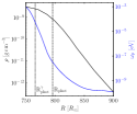
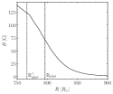
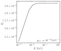
Figure S5: (Left) Average density and plasma frequency from the RSG hydrodynamic simulation RSG1L4.5 in Ref. Goldberg et al. (2022). We mark the photosphere radius and the radius from which 100 MeV gamma-rays typically free-stream outwards without scattering, $R_{\rm phot}^{\gamma}$. (Center) Our inferred magnetic field strength as a function of the radius $R$ within the star, assuming equipartition between the magnetic energy density and the kinetic energy density in convection. (Right) The axion-to-photon conversion probability (for low axion masses $m_{a}\sim 0$ eV) as a function of the axion energy $E$, assuming $g_{a\gamma\gamma}=10^{-12}$ GeV^-1 for illustration.

V SN Simulations: Intermediate Quantities

In this section we provide additional information related to the SN simulations used in this work from Ref. Bollig et al. (2020). Figure S6, Fig. S7 and Fig. S8 show the radial dependence of the temperature, density profiles, and proton mass along with chemical potentials (note that for nucleons we show the non-relativistic chemical potentials), respectively, across the three simulations considered in this work. Figure S9 shows the gravitational redshift $z$ (more precisely, we illustrate $(1+z)^{-1}$) due to the extreme densities reached in the SN core. These quantities are used to compute the axion emissivity.

In this work, we assume a thermal distribution of pions, with a chemical potential dictated by weak equilibrium, $\mu_{\pi^{-}}=\mu_{e}-\mu_{\nu_{e}}$. Note that the modeling of the pion abundance in dense nuclear matter is still an open question. The main uncertainties concern the presence and description of a Bose-Einstein condensation phase Migdal et al. (1990) as well as the effects of pion-nucleon interactions on the pion dispersion relation Fore and Reddy (2020); Carenza et al. (2021); Fore et al. (2023). Ultimately, dedicated SN simulations accounting for pions are needed to properly assess their impact on the SN thermodynamical evolution and axion luminosity.

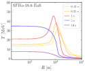
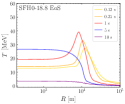
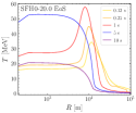
Figure S6: Temperature Profiles as a function of the radius $R$ within the PNS at different times for the three SN simulations used in this work.

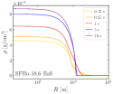
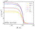
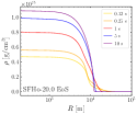
Figure S7: As in Fig. S6 but for the nuclear density profiles.

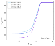
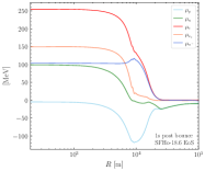
Figure S8: Profiles of the proton mass (left) and chemical potentials (right) at 1 s after the core collapse in the PNS. In the left panel we illustrate the results across the three simulations considered, while in the right panel we show results for our fiducial simulation SFHo-18.6.

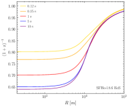
Figure S9: Profiles of $(1+z)^{-1}$, where $z$ is the gravitational redshift, obtained with our fiducial SN simulation SFH0-18.6 EoS, for different times after the SN explosion.

VI Solar Maximum Mission Analysis and Comparison to GALAXIS / Fermi-LAT

We use the SN1987A data from the SMM provided in Hoof and Schulz (2023) for the energy bins 4.1-6.4 MeV, 10-25 MeV, and 25-100 MeV, with time binned in $\Delta t=2.048$ s intervals. We model the data using a Poisson likelihood. For the background model contribution we use a linear ansatz of the form

$$\mu^{\mathrm{bkg}}_{i,j}=b^{(0)}_{j}+b^{(1)}_{j}\frac{t_{i}-t_{\nu}}{\Delta t}\,,$$ (S34)

where $t_{i}$ corresponds to the $i^{\rm th}$ time bin and $j$ corresponds to the index over the three energy bins. The six parameters $\{b_{j}^{(0)},b_{j}^{(1)}\}_{j=1}^{3}$ are the background nuisance parameters. For the signal model, with mean prediction $\mu_{i,j}^{\rm sig}$, we take the axion emission spectrum and calculate the mean expected photon counts by convolving with the instrument response:

$$\mu^{\mathrm{sig}}_{i,j}=\frac{A_{\mathrm{eff},j}}{4\pi d^{2}}\int_{E_{j}}^{E^{\prime}_{j}}dE_{a}\int_{t_{i}}^{t^{\prime}_{i}}dt\,P_{a\gamma}(g_{a\gamma\gamma},m_{a},E_{a})\frac{d^{2}N_{a}(g_{a\gamma\gamma},E_{a},t)}{dtdE_{a}}\,,$$ (S35)

where $P_{a\gamma}$ corresponds to the conversion probability of axions-to-photons, $d$ is the distance to the SN, $d^{2}N_{a}/dt/dE_{a}$ is the differential number of axions generated by the PNS per unit time per unit energy, $A_{{\rm eff},j}$ is the SMM effective area in energy bin $j$, and $E_{j}$ $E^{\prime}_{j}$ ($t_{i}$ $t^{\prime}_{i}$) are the values of the bin edges for the $j^{\rm th}$ energy ($i^{\rm th}$ time) bin. The values of $A_{{\rm eff},j}$ are approximately $28,115,63$ cm² in energy bins $j=1,2,3$, respectively. In Fig. S10 we illustrate the SMM effective area and compare it to that of the Fermi-LAT. Note that we assume the proposed GALAXIS constellation has the same effective area as the Fermi-LAT but with full-sky angular coverage. In addition to gaining in effective area, the Fermi-LAT also has significantly improved background rate with respect to SMM. For Fermi-LAT (and thus also for GALAXIS) we project zero background events within the $\sim$10 s of the SN event, while for SMM the number of background events was around 50 events per 10 s.

Note, also, that while we assume that the GALAXIS network will have $4\pi$ angular coverage, it is possible that the network could still have a high chance of detecting the next Galactic SN with slightly less angular coverage, considering that the next SN will likely lie in the Galactic plane. We leave a technical optimization of the sky coverage for future work.

We analyze the data using the joint signal plus background model, fixing the start of the SN to the observed time from the neutrino burst. We include data from $\sim$150 s before the event until $\sim$220 s afterwards. At fixed $m_{a}$ we compute the profile likelihood as a function of the signal strength parameter $g_{a\gamma\gamma}$ profiling over the background nuisance parameters. Note that for consistency, to account for downward fluctuations, we also allow for negative signal strengths; we then use Wilks’ theorem, relying on the observation that the numbers of counts per bin are typically above 10, to set the 95% upper limits and compute the discovery test statistics (see, e.g., Safdi (2022)).

The data are illustrated in Fig. S11 along with the best-fit signal plus background model for the axion-like particle scenario with $m_{a}=0$ eV accounting for conversion on the stellar magnetic field with $B_{0}=1$ kG; the best-fit coupling is $g_{a\gamma\gamma}=5.6\times 10^{-12}$ GeV^-1 in that case, with discovery test statistic ${\rm TS}\approx 0.3$.

Figure S10: The effective area as a function of energy for both Fermi-LAT (P8R3_TRANSIENT020_V2 event class) and SMM. In our projections we assume that the proposed GALAXIS instrument has the Fermi-LAT on-axis instrument response but with $4\pi$ angular coverage.

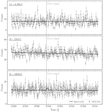
Figure S11: The SMM data provided in Hoof and Schulz (2023) in the three energy bins within the time-frame of SN1987A. We illustrate the best-fit signal plus background model at $m_{a}=0$ accounting for axion-to-photon conversion on the stellar magnetic field of the progenitor star, assuming $B_{0}=1$ kG; in this case the best-fit coupling strength is $g_{a\gamma\gamma}\approx 5.6\times 10^{-12}$ GeV^-1 and the discovery test statistic is ${\rm TS}\approx 0.3$.

VII Analysis Variation

In this section we summarize a number of analysis variations that are aimed to assess the robustness of the results presented in the main Letter. First, in Fig. S12 we show comparisons of the differential axion spectra, integrated over time, for Primakoff, bremsstrahlung and pion conversion, obtained with the three different simulations discussed in Sec. V. Pion conversion dominates in all cases, though there is roughly an order of magnitude spread in the predicted spectra across the simulations. In Fig. S13 (top panel) we show the mean differential number of axions generated in the PNS, integrated over energy, as a function of time for our fiducial SN simulation. We again separately break down the contributions from Primakoff, bremsstrahlung and pion conversion. The bottom panel of Fig. S13 illustrates the mean energy $\langle E_{a}\rangle$ of axions emitted from the SN for each process. The pion conversion processes emit more energetic axions than Primakoff and bremsstrahlung.

In Fig. S14 we compare the SN1987A limits obtained using different models for the Galactic magnetic field (see Sec. IV.a for a discussion). These limits are obtained with the simulation SFHo-18.6, assuming a BSG progenitor star with a radius of 45 $R_{\odot}$ as in our fiducial limits. On the other hand, in Fig. S15 we consider our fiducial SN1987A scenario but vary the surface magnetic field $B_{0}$ from 100 G to 10 kG to, broadly, encapsulate the uncertainty in the magnetic field for a typical BSG. (Note that the 100 G assumption leads to the weakest limits, with 10 kG giving the strongest results.) We also show, as in Fig. 1, the projections for a next BSG Galactic SN. The analogous results obtained with the three different SN simulations, assuming a BSG progenitor star with a radius of 45 $R_{\odot}$ and a magnetic field at the surface of the star of 1 kG, are shown in Fig. S16.

In Fig. S17 we project the upper limits under the null hypothesis, as in Fig. 1, but assuming a RSG progenitor. As discussed more in Sec. IV.b, RSGs are more likely core-collapse SN progenitors than BSGs, but their magnetic field distributions are more uncertain as the relevant fields arise dynamically from the conducting fluid dynamics in the outer layers of the star.

Given the uncertainties in the pion-conversion processes, it is instructive to illustrate projected upper limits with GALAXIS for the next Galactic SN assuming no pion-induced emission processes. As seen in Fig. S18, including pions does not strongly affect the low-mass sensitivity and has a slightly more pronounced affect at higher masses, since the pions give rise to higher-energy axions relative to e.g. bremsstrahlung processes. Note that pion emission is not relevant for SN1987A given the limited energy range of the SMM instrumentation.

Lastly, it is useful to rephrase our limits from SN1987A in terms of limits in the space of $g_{a\gamma\gamma}$, $g_{ann}$, and $g_{app}$ without assuming any relations between these EFT parameters. However, to simplify the parameter space we assume $m_{a}\ll 10^{-10}$ eV so that we may neglect the axion mass when computing the Galactic axion-to-photon conversion probabilities. The limits illustrated in Fig. 1 may then be expanded into limits on $g_{a\gamma\gamma}$-$g_{ann}$ (assuming $g_{app}=0$) and $g_{a\gamma\gamma}$-$g_{app}$ (assuming $g_{ann}=0$); see Fig. S19. These new upper limits computed in this work surpass those on the axion-photon coupling only (e.g., Reynés et al. (2021); Ning and Safdi (2024)) and the nucleon couplings only (e.g., Buschmann et al. (2022)) for some of the parameter space.

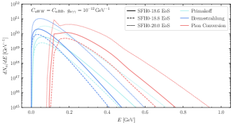
Figure S12: The differential axion spectra, integrated over the first 10 s after the core collapse, obtained from different processes, using the three SN simulations discussed in Sec. V. Note that we assume $C_{aWW}=C_{aBB}$ and take $g_{a\gamma\gamma}=10^{-12}$ GeV^-1 for definiteness in this figure.

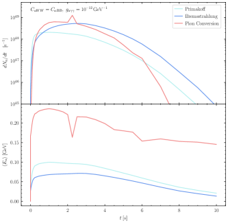
Figure S13: (Top panel) The time dependence of the axion luminosity, integrated over energy for the different production mechanisms discussed. We illustrate these results for our fiducial SN simulation (SFH0-18.6 EoS). (Bottom panel) The average energy of emitted axions broken up by production mechanism. Pionic processes result in more energetic axions. The sharp feature in the pion emission around $t\sim 2$ s is due to an incorrect, but also insignificant, description of the pion condensate in our formalism (see text for details).

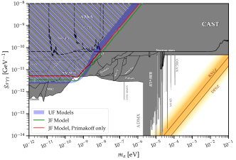
Figure S14: As in Fig. 1 for the low-mass SN1987A limits accounting for axion-to-photon conversion on the Galactic magnetic fields, but varying over magnetic fields models. Note that for the 8 UF models we shade the range of upper limits found across those models; our fiducial limit is, at each $m_{a}$, taken to be the weakest across that ensemble.

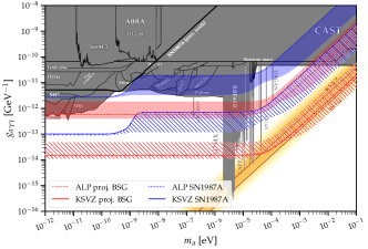
Figure S15: As in Fig. 1 but only showing the results for conversion on the stellar magnetic field and varying the magnetic field strength at the surface of the BSG between $B_{0}=100$ G and $B_{0}=10$ kG.

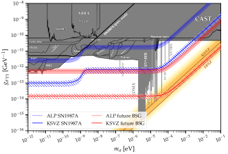
Figure S16: As in Fig. 1 but varying between the three SN simulations discussed in this work, with all other parameters as in Fig. 1. The stronger limits arise from more massive PNSs. The curves within the shaded regions show the fiducial results used in Fig. 1.

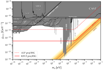
Figure S17: As in Fig. 1 but only showing projections for the next Galactic SN and assuming a RSG progenitor at 10 kpc from Earth instead of a BSG progenitor. The RSG projections are slightly less strong than those for the BSG, though we stress that the RSG results are subject to large uncertainties on the magnetic field modeling.

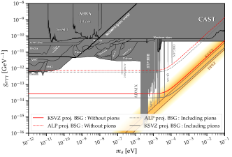
Figure S18: As in Fig. 1 for future SN projections with GALAXIS including (as we do in our fiducial calculations) or removing the axion production from axion-pion conversion.

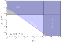
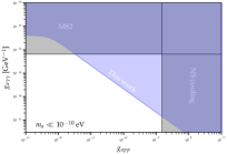
Figure S19: Upper limits computed in this work on the EFT parameter space $g_{a\gamma\gamma}-g_{ann}$, with $g_{app}=0$ (left panel), and $g_{a\gamma\gamma}-g_{app}$, with $g_{ann}=0$ (right panel), from the non-observation of gamma-rays from SN1987A. We account for axion-to-photon conversion in the Galactic magnetic field and assume $m_{a}\ll 10^{-10}$ eV such that the axion mass does not play a role in the axion-photon conversion process. Our new upper limits exclude previously allowed regions of the illustrated parameter space.

VIII Neutron star merger estimates

In the main Letter we focus on axion-induced gamma-ray signals from PNSs formed after core-collapse SN. On the other hand, it is also interesting to consider similar signals created from the hot PNSs formed after NS mergers. A key difference between SN and NS mergers for the signal of interest is that for SN the axions must escape the much larger surrounding star before converting to gamma-rays, while for NS mergers axions may immediately begin to convert to gamma-rays after exiting the PNS.

Modeling the axion-induced gamma-ray signal from NS mergers would require dedicated simulations to accurately model the PNS interior and the magnetic field distributions. Such simulations, incorporating axion emission, would be an interesting direction for future work. Here, on the other hand, we apply more basic approximations in order to show that NS mergers are potentially promising targets for axion searches in gamma-rays.

The first approximation we make in this work is that the integrated (over time) differential (in terms of energy) flux of axions produced during a NS merger matches that in our default SN simulation. This approximation is almost certainly not correct in detail, but we may roughly compare the predicted axion luminosities between SN and NS-merger remnants through the following argument. The axion luminosities from nuclear matter in the degenerate limit roughly scale as $T^{6}$ (see SM Secs. I.c and I.b). A NS remnant may have a maximum temperature $\sim$40-60 MeV for a time of around 1 s (see, e.g., Fig. S6). On the other hand, the remnants formed immediently before and during NS mergers can have much higher temperatures over shorter periods of time.

NS mergers may result in black holes or in stable NS remnants. In the case of black hole formation, the hypermassive remnant still exists for $\sim$20 ms after merger, until angular momentum loss from gravitational wave radiation causes the remnant to collapse (see, e.g., Kiuchi et al. (2023) and references therein). During the initial $\sim$10 ms the temperature can potentially surpass 100 MeV regardless of whether the remnant is stable or not Hanauske et al. (2019); Dietrich and Clough (2019); Zappa et al. (2022); Kiuchi et al. (2023); Radice and Bernuzzi (2023). We may then roughly estimate the axion luminosity of a NS merger, regardless of the final state, relative to that from a SN by $(100\,\,{\rm MeV}/50\,\,{\rm MeV})^{6}\times(10\,\,{\rm ms}/1\,\,{\rm s})\sim 0.6$. That is, even though remnants from NS mergers (for example, those collapsing to black holes) may also survive for fractions of a second, the high temperatures reached in these dense systems can potentially lead to axion luminosities comparable to those found in the PNSs formed after SN. Of course, the estimate above is extremely rough, but it justifies – on a first pass – using a SN simulation to model the remnant formed after the NS merger. A more accurate projection would used dedicated NS merger simulations, which we leave for future work.

As a very rough approximation to a NS merger, we thus use our SN simulation SFHo-20.0, which results in the most massive remnant of our SN simulation suite. (Again, we caution that this is not an accurate simulations of a NS merger.) In Fig. S20 we project the sensitivity of Fermi-LAT (or our proposed GALAXIS) to the axion-signal from a NS merger using the SFHo-20.0 simulation to describe the remnant evolution. We assume a distance of 30 Mpc to the NS merger. This distance estimate is motivated by e.g. the 2017 NS merger resulting in the gravitational wave signal GW170817 detected by LIGO Abbott et al. (2018); this event originated $\sim$40 Mpc from Earth. Events at $\sim$30 Mpc may potentially be expected around once per 10 years Abbott et al. (2019). (Note that the upper limits on $g_{a\gamma\gamma}$ scale with the distance to the SN as $g_{a\gamma\gamma}\propto\sqrt{d}$, so the difference between 30 Mpc and e.g. 50 Mpc is relatively minor.)

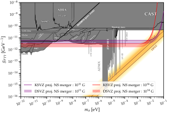
Figure S20: Projected 95% upper limits under the null hypothesis on $g_{a\gamma\gamma}$ from an observation of Fermi / GALAXIS towards a NS-NS merger at a distance of 30 Mpc. As a rough estimate, we use the SFHo-20.0 SN simulation to describe the remnant from the merger. We also model the magnetic field of the remnant as a dipole with surface field strengths as indicated (we consider two possibilities). These approximations are rough but motivate future work that more accurately computes the axion-induced signal from NS mergers.

In Fig. S20 we model the magnetic field of the remnant as a centered dipole with surface field strength (at a radius $r_{0}=10$ km) of $B_{0}=10^{11}$ G and $B_{0}=10^{14}$ G. The first choice of field is motivated by the typical magnetic field strength of older NSs, while the second accounts for the expected amplification in NS mergers. In fact, magnetic fields can be amplified during the NS merger to well above $\sim$$10^{15}$ G Combi and Siegel (2023). Moreover, the magnetic fields generated during this amplification are not regular but turbulent, which would increase the conversion probability for high-mass axions by giving the B-field non-trivial spatial dependence. Still, for the purpose of the simple estimates in this work we adopt the dipole field configurations. Then, we compute the axion-to-photon conversion probabilities using the approximate analytic relations in Fortin et al. (2021). We illustrate both KSVZ and DFSZ sensitivities in Fig. S20; to conclude, we note that due to the compact nature of these remnants the projected upper limits become tantalizingly close to probing the QCD axion for masses $m_{a}\sim 10^{-3}-10^{-2}$ eV, motivating incorporating axions into dedicated simulations.

References

- Hirata et al. (1987) K. Hirata et al. (Kamiokande-II), “Observation of a Neutrino Burst from the Supernova SN 1987a,” Phys. Rev. Lett. 58, 1490–1493 (1987).
- Bionta et al. (1987) R. M. Bionta et al., “Observation of a Neutrino Burst in Coincidence with Supernova SN 1987a in the Large Magellanic Cloud,” Phys. Rev. Lett. 58, 1494 (1987).
- Alekseev et al. (1987) E. N. Alekseev, L. N. Alekseeva, V. I. Volchenko, and I. V. Krivosheina, “Possible Detection of a Neutrino Signal on 23 February 1987 at the Baksan Underground Scintillation Telescope of the Institute of Nuclear Research,” JETP Lett. 45, 589–592 (1987).
- Raffelt (1996) G. G. Raffelt, Stars as laboratories for fundamental physics: The astrophysics of neutrinos, axions, and other weakly interacting particles (1996).
- Raffelt (1990) Georg G. Raffelt, “Astrophysical methods to constrain axions and other novel particle phenomena,” Phys. Rept. 198, 1–113 (1990).
- Brockway et al. (1996) Jack W. Brockway, Eric D. Carlson, and Georg G. Raffelt, “SN1987A gamma-ray limits on the conversion of pseudoscalars,” Phys. Lett. B 383, 439–443 (1996), arXiv:astro-ph/9605197 .
- Grifols et al. (1996) J. A. Grifols, E. Masso, and R. Toldra, “Gamma-rays from SN1987A due to pseudoscalar conversion,” Phys. Rev. Lett. 77, 2372–2375 (1996), arXiv:astro-ph/9606028 .
- Payez et al. (2015) Alexandre Payez, Carmelo Evoli, Tobias Fischer, Maurizio Giannotti, Alessandro Mirizzi, and Andreas Ringwald, “Revisiting the SN1987A gamma-ray limit on ultralight axion-like particles,” JCAP 02, 006 (2015), arXiv:1410.3747 [astro-ph.HE] .
- Hoof and Schulz (2023) Sebastian Hoof and Lena Schulz, “Updated constraints on axion-like particles from temporal information in supernova SN1987A gamma-ray data,” JCAP 03, 054 (2023), arXiv:2212.09764 [hep-ph] .
- Caputo and Raffelt (2024) Andrea Caputo and Georg Raffelt, “Astrophysical Axion Bounds: The 2024 Edition,” in 1st Training School of the COST Action COSMIC WISPers (CA21106) (2024) arXiv:2401.13728 [hep-ph] .
- Page et al. (2020) Dany Page, Mikhail V. Beznogov, Iván Garibay, James M. Lattimer, Madappa Prakash, and Hans-Thomas Janka, “NS 1987A in SN 1987A,” Astrophys. J. 898, 125 (2020), arXiv:2004.06078 [astro-ph.HE] .
- Fransson et al. (2024) C. Fransson et al., “Emission lines due to ionizing radiation from a compact object in the remnant of Supernova 1987A,” Science 383, 898–903 (2024), arXiv:2403.04386 [astro-ph.HE] .
- Reynolds et al. (2020) Christopher S. Reynolds, M. C. David Marsh, Helen R. Russell, Andrew C. Fabian, Robyn Smith, Francesco Tombesi, and Sylvain Veilleux, “Astrophysical limits on very light axion-like particles from Chandra grating spectroscopy of NGC 1275,” Astrophys. J. 890, 59 (2020), arXiv:1907.05475 [hep-ph] .
- Dessert et al. (2020) Christopher Dessert, Joshua W. Foster, and Benjamin R. Safdi, “X-ray Searches for Axions from Super Star Clusters,” Phys. Rev. Lett. 125, 261102 (2020), arXiv:2008.03305 [hep-ph] .
- Reynés et al. (2021) Júlia Sisk Reynés, James H. Matthews, Christopher S. Reynolds, Helen R. Russell, Robyn N. Smith, and M. C. David Marsh, “New constraints on light axion-like particles using Chandra transmission grating spectroscopy of the powerful cluster-hosted quasar H1821+643,” Mon. Not. Roy. Astron. Soc. 510, 1264–1277 (2021), arXiv:2109.03261 [astro-ph.HE] .
- Noordhuis et al. (2023) Dion Noordhuis, Anirudh Prabhu, Samuel J. Witte, Alexander Y. Chen, Fábio Cruz, and Christoph Weniger, “Novel Constraints on Axions Produced in Pulsar Polar-Cap Cascades,” Phys. Rev. Lett. 131, 111004 (2023), arXiv:2209.09917 [hep-ph] .
- Dessert et al. (2022) Christopher Dessert, David Dunsky, and Benjamin R. Safdi, “Upper limit on the axion-photon coupling from magnetic white dwarf polarization,” Phys. Rev. D 105, 103034 (2022), arXiv:2203.04319 [hep-ph] .
- Dolan et al. (2022) Matthew J. Dolan, Frederick J. Hiskens, and Raymond R. Volkas, “Advancing globular cluster constraints on the axion-photon coupling,” JCAP 10, 096 (2022), arXiv:2207.03102 [hep-ph] .
- Davies et al. (2023) James Davies, Manuel Meyer, and Garret Cotter, “Constraints on axionlike particles from a combined analysis of three flaring Fermi flat-spectrum radio quasars,” Phys. Rev. D 107, 083027 (2023), arXiv:2211.03414 [astro-ph.HE] .
- Ning and Safdi (2024) Orion Ning and Benjamin R. Safdi, “Leading Axion-Photon Sensitivity with NuSTAR Observations of M82 and M87,” (2024), arXiv:2404.14476 [hep-ph] .
- O’HARE (2020) Ciaran O’HARE, “cajohare/axionlimits: Axionlimits,” (2020).
- Workman and Others (2022) R. L. Workman and Others (Particle Data Group), “Review of Particle Physics,” PTEP 2022, 083C01 (2022).
- Peccei and Quinn (1977a) R. D. Peccei and Helen R. Quinn, “CP Conservation in the Presence of Instantons,” Phys. Rev. Lett. 38, 1440–1443 (1977a).
- Peccei and Quinn (1977b) R. D. Peccei and Helen R. Quinn, “Constraints Imposed by CP Conservation in the Presence of Instantons,” Phys. Rev. D16, 1791–1797 (1977b).
- Weinberg (1978) Steven Weinberg, “A New Light Boson?” Phys. Rev. Lett. 40, 223–226 (1978).
- Wilczek (1978) Frank Wilczek, “Problem of Strong p and t Invariance in the Presence of Instantons,” Phys. Rev. Lett. 40, 279–282 (1978).
- Preskill et al. (1983) John Preskill, Mark B. Wise, and Frank Wilczek, “Cosmology of the Invisible Axion,” Phys. Lett. 120B, 127–132 (1983).
- Abbott and Sikivie (1983) L. F. Abbott and P. Sikivie, “A Cosmological Bound on the Invisible Axion,” Phys. Lett. 120B, 133–136 (1983).
- Dine and Fischler (1983) Michael Dine and Willy Fischler, “The Not So Harmless Axion,” Phys. Lett. 120B, 137–141 (1983).
- Svrcek and Witten (2006) Peter Svrcek and Edward Witten, “Axions In String Theory,” JHEP 06, 051 (2006), arXiv:hep-th/0605206 [hep-th] .
- Arvanitaki et al. (2010) Asimina Arvanitaki, Savas Dimopoulos, Sergei Dubovsky, Nemanja Kaloper, and John March-Russell, “String Axiverse,” Phys. Rev. D81, 123530 (2010), arXiv:0905.4720 [hep-th] .
- Cicoli et al. (2012) Michele Cicoli, Mark Goodsell, and Andreas Ringwald, “The type IIB string axiverse and its low-energy phenomenology,” JHEP 10, 146 (2012), arXiv:1206.0819 [hep-th] .
- Demirtas et al. (2020) Mehmet Demirtas, Cody Long, Liam McAllister, and Mike Stillman, “The Kreuzer-Skarke Axiverse,” JHEP 04, 138 (2020), arXiv:1808.01282 [hep-th] .
- Halverson et al. (2019) James Halverson, Cody Long, Brent Nelson, and Gustavo Salinas, “Towards string theory expectations for photon couplings to axionlike particles,” Phys. Rev. D 100, 106010 (2019), arXiv:1909.05257 [hep-th] .
- Demirtas et al. (2021) Mehmet Demirtas, Naomi Gendler, Cody Long, Liam McAllister, and Jakob Moritz, “PQ Axiverse,” (2021), arXiv:2112.04503 [hep-th] .
- Raffelt and Seckel (1988) Georg Raffelt and David Seckel, “Bounds on Exotic Particle Interactions from SN 1987a,” Phys. Rev. Lett. 60, 1793 (1988).
- Ellis and Olive (1987) John Ellis and K. A. Olive, “Constraints on light particles from supernova SN 1987A,” Physics Letters B 193, 525–530 (1987).
- Turner (1988) Michael S. Turner, “Axions from SN 1987a,” Phys. Rev. Lett. 60, 1797 (1988).
- Mayle et al. (1988) Ron Mayle, James R. Wilson, John Ellis, Keith Olive, David N. Schramm, and Gary Steigman, “Constraints on axions from SN 1987A,” Physics Letters B 203, 188–196 (1988).
- Mayle et al. (1996) Ron Mayle, James R. Wilson, John Ellis, Keith A. Olive, David N. Schramm, and Gary Steigman, “Updated Constraints on Axions from SN1987A,” in The Big Bang and Other Explosions in Nuclear and Particle Astrophysics. Edited by SCHRAMM DAVID N. Published by World Scientific Publishing Co. Pte. Ltd (1996) pp. 188–193.
- Brinkmann and Turner (1988) Ralf Peter Brinkmann and Michael S. Turner, “Numerical Rates for Nucleon-Nucleon Axion Bremsstrahlung,” Phys. Rev. D 38, 2338 (1988).
- Burrows et al. (1989) Adam Burrows, Michael S. Turner, and R. P. Brinkmann, “Axions and SN 1987a,” Phys. Rev. D 39, 1020 (1989).
- Janka et al. (1996) Hans-Thomas Janka, Wolfgang Keil, Georg Raffelt, and David Seckel, “Nucleon spin fluctuations and the supernova emission of neutrinos and axions,” Phys. Rev. Lett. 76, 2621–2624 (1996), arXiv:astro-ph/9507023 .
- Keil et al. (1997) Wolfgang Keil, Hans-Thomas Janka, David N. Schramm, Gunter Sigl, Michael S. Turner, and John R. Ellis, “A Fresh look at axions and SN-1987A,” Phys. Rev. D 56, 2419–2432 (1997), arXiv:astro-ph/9612222 .
- Fischer et al. (2016) Tobias Fischer, Sovan Chakraborty, Maurizio Giannotti, Alessandro Mirizzi, Alexandre Payez, and Andreas Ringwald, “Probing axions with the neutrino signal from the next galactic supernova,” Phys. Rev. D 94, 085012 (2016), arXiv:1605.08780 [astro-ph.HE] .
- Carenza et al. (2019) Pierluca Carenza, Tobias Fischer, Maurizio Giannotti, Gang Guo, Gabriel Martínez-Pinedo, and Alessandro Mirizzi, “Improved axion emissivity from a supernova via nucleon-nucleon bremsstrahlung,” JCAP 10, 016 (2019), [Erratum: JCAP 05, E01 (2020)], arXiv:1906.11844 [hep-ph] .
- Lella et al. (2024a) Alessandro Lella, Pierluca Carenza, Giampaolo Co’, Giuseppe Lucente, Maurizio Giannotti, Alessandro Mirizzi, and Thomas Rauscher, “Getting the most on supernova axions,” Phys. Rev. D 109, 023001 (2024a), arXiv:2306.01048 [hep-ph] .
- Manzari et al. (2023) Claudio Andrea Manzari, Jorge Martin Camalich, Jonas Spinner, and Robert Ziegler, “Supernova limits on muonic dark forces,” Phys. Rev. D 108, 103020 (2023), arXiv:2307.03143 [hep-ph] .
- Meyer et al. (2017) M. Meyer, M. Giannotti, A. Mirizzi, J. Conrad, and M.A. Sánchez-Conde, “Fermi Large Area Telescope as a Galactic Supernovae Axionscope,” Phys. Rev. Lett. 118, 011103 (2017), arXiv:1609.02350 [astro-ph.HE] .
- Calore et al. (2024) Francesca Calore, Pierluca Carenza, Christopher Eckner, Maurizio Giannotti, Giuseppe Lucente, Alessandro Mirizzi, and Francesco Sivo, “Uncovering axionlike particles in supernova gamma-ray spectra,” Phys. Rev. D 109, 043010 (2024), arXiv:2306.03925 [astro-ph.HE] .
- Forrest et al. (1980) D. J. Forrest, E. L. Chupp, J. M. Ryan, M. L. Cherry, I. U. Gleske, C. Reppin, K. Pinkau, E. Rieger, G. Kanbach, R. L. Kinzer, G. Share, W. N. Johnson, and J. D. Kurfess, “The gamma ray spectrometer for the Solar Maximum Mission.” Sol. Phys. 65, 15–23 (1980).
- Carenza et al. (2021) Pierluca Carenza, Bryce Fore, Maurizio Giannotti, Alessandro Mirizzi, and Sanjay Reddy, “Enhanced Supernova Axion Emission and its Implications,” Phys. Rev. Lett. 126, 071102 (2021), arXiv:2010.02943 [hep-ph] .
- Fischer et al. (2021) Tobias Fischer, Pierluca Carenza, Bryce Fore, Maurizio Giannotti, Alessandro Mirizzi, and Sanjay Reddy, “Observable signatures of enhanced axion emission from protoneutron stars,” Phys. Rev. D 104, 103012 (2021), arXiv:2108.13726 [hep-ph] .
- Choi et al. (2022) Kiwoon Choi, Hee Jung Kim, Hyeonseok Seong, and Chang Sub Shin, “Axion emission from supernova with axion-pion-nucleon contact interaction,” JHEP 02, 143 (2022), arXiv:2110.01972 [hep-ph] .
- Vonk et al. (2022) Thomas Vonk, Feng-Kun Guo, and Ulf-G. Meißner, “Pion axioproduction: The resonance contribution,” Phys. Rev. D 105, 054029 (2022), arXiv:2202.00268 [hep-ph] .
- Ho et al. (2023) Shu-Yu Ho, Jongkuk Kim, Pyungwon Ko, and Jae-hyeon Park, “Supernova axion emissivity with (1232) resonance in heavy baryon chiral perturbation theory,” Phys. Rev. D 107, 075002 (2023), arXiv:2212.01155 [hep-ph] .
- Bollig et al. (2020) Robert Bollig, William DeRocco, Peter W. Graham, and Hans-Thomas Janka, “Muons in supernovae: implications for the axion-muon coupling,” Phys. Rev. Lett. 125, 051104 (2020), arXiv:2005.07141 [hep-ph] .
- Janka (2012) Hans-Thomas Janka, “Explosion Mechanisms of Core-Collapse Supernovae,” Ann. Rev. Nucl. Part. Sci. 62, 407–451 (2012), arXiv:1206.2503 [astro-ph.SR] .
- Bollig et al. (2017) R. Bollig, H. Th. Janka, A. Lohs, G. Martinez-Pinedo, C. J. Horowitz, and T. Melson, “Muon Creation in Supernova Matter Facilitates Neutrino-driven Explosions,” Phys. Rev. Lett. 119, 242702 (2017), arXiv:1706.04630 [astro-ph.HE] .
- Chang and Choi (1993) Sanghyeon Chang and Kiwoon Choi, “Hadronic axion window and the big bang nucleosynthesis,” Phys. Lett. B 316, 51–56 (1993), arXiv:hep-ph/9306216 .
- Vonk et al. (2021) Thomas Vonk, Feng-Kun Guo, and Ulf-G. Meißner, “The axion-baryon coupling in SU(3) heavy baryon chiral perturbation theory,” JHEP 08, 024 (2021), arXiv:2104.10413 [hep-ph] .
- Kim (1979) Jihn E. Kim, “Weak Interaction Singlet and Strong CP Invariance,” Phys. Rev. Lett. 43, 103 (1979).
- Shifman et al. (1980) Mikhail A. Shifman, A. I. Vainshtein, and Valentin I. Zakharov, “Can Confinement Ensure Natural CP Invariance of Strong Interactions?” Nucl. Phys. B 166, 493–506 (1980).
- Dine et al. (1981) Michael Dine, Willy Fischler, and Mark Srednicki, “A Simple Solution to the Strong CP Problem with a Harmless Axion,” Phys. Lett. B 104, 199–202 (1981).
- Zhitnitsky (1980) A. R. Zhitnitsky, “On Possible Suppression of the Axion Hadron Interactions. (In Russian),” Sov. J. Nucl. Phys. 31, 260 (1980).
- Bauer et al. (2022) Martin Bauer, Matthias Neubert, Sophie Renner, Marvin Schnubel, and Andrea Thamm, “Flavor probes of axion-like particles,” JHEP 09, 056 (2022), arXiv:2110.10698 [hep-ph] .
- Raffelt (1986) Georg G. Raffelt, “Astrophysical Axion Bounds Diminished by Screening Effects,” Phys. Rev. D 33, 897 (1986).
- (68) “Garching Core-Collapse Supernova archive,” https://wwwmpa.mpa-garching.mpg.de/ccsnarchive/.
- Fiorillo et al. (2023) Damiano F. G. Fiorillo, Malte Heinlein, Hans-Thomas Janka, Georg Raffelt, Edoardo Vitagliano, and Robert Bollig, “Supernova simulations confront SN 1987A neutrinos,” Phys. Rev. D 108, 083040 (2023), arXiv:2308.01403 [astro-ph.HE] .
- Mirizzi et al. (2016) Alessandro Mirizzi, Irene Tamborra, Hans-Thomas Janka, Ninetta Saviano, Kate Scholberg, Robert Bollig, Lorenz Hudepohl, and Sovan Chakraborty, “Supernova Neutrinos: Production, Oscillations and Detection,” Riv. Nuovo Cim. 39, 1–112 (2016), arXiv:1508.00785 [astro-ph.HE] .
- Rampp and Janka (2002) Markus Rampp and H. Thomas Janka, “Radiation hydrodynamics with neutrinos: Variable Eddington factor method for core collapse supernova simulations,” Astron. Astrophys. 396, 361 (2002), arXiv:astro-ph/0203101 .
- Fischer et al. (2014) Tobias Fischer, Matthias Hempel, Irina Sagert, Yudai Suwa, and Jürgen Schaffner-Bielich, “Symmetry energy impact in simulations of core-collapse supernovae,” Eur. Phys. J. A 50, 46 (2014), arXiv:1307.6190 [astro-ph.HE] .
- Oertel et al. (2017) M. Oertel, M. Hempel, T. Klähn, and S. Typel, “Equations of state for supernovae and compact stars,” Rev. Mod. Phys. 89, 015007 (2017), arXiv:1610.03361 [astro-ph.HE] .
- Fischer et al. (2017) Tobias Fischer, Niels-Uwe Bastian, David Blaschke, Mateusz Cierniak, Matthias Hempel, Thomas Klähn, Gabriel Martínez-Pinedo, William G. Newton, Gerd Röpke, and Stefan Typel, “The state of matter in simulations of core-collapse supernovae – Reflections and recent developments,” Publ. Astron. Soc. Austral. 34, 67 (2017), arXiv:1711.07411 [astro-ph.HE] .
- Demorest et al. (2010) Paul Demorest, Tim Pennucci, Scott Ransom, Mallory Roberts, and Jason Hessels, “Shapiro Delay Measurement of A Two Solar Mass Neutron Star,” Nature 467, 1081–1083 (2010), arXiv:1010.5788 [astro-ph.HE] .
- Antoniadis et al. (2013) John Antoniadis et al., “A Massive Pulsar in a Compact Relativistic Binary,” Science 340, 6131 (2013), arXiv:1304.6875 [astro-ph.HE] .
- Cromartie et al. (2019) H. T. Cromartie et al. (NANOGrav), “Relativistic Shapiro delay measurements of an extremely massive millisecond pulsar,” Nature Astron. 4, 72–76 (2019), arXiv:1904.06759 [astro-ph.HE] .
- Abbott et al. (2018) B. P. Abbott et al. (LIGO Scientific, Virgo), “GW170817: Measurements of neutron star radii and equation of state,” Phys. Rev. Lett. 121, 161101 (2018), arXiv:1805.11581 [gr-qc] .
- Bauswein et al. (2017) Andreas Bauswein, Oliver Just, Hans-Thomas Janka, and Nikolaos Stergioulas, “Neutron-star radius constraints from GW170817 and future detections,” Astrophys. J. Lett. 850, L34 (2017), arXiv:1710.06843 [astro-ph.HE] .
- Essick et al. (2020) Reed Essick, Ingo Tews, Philippe Landry, Sanjay Reddy, and Daniel E. Holz, “Direct Astrophysical Tests of Chiral Effective Field Theory at Supranuclear Densities,” Phys. Rev. C 102, 055803 (2020), arXiv:2004.07744 [astro-ph.HE] .
- Hook (2018) Anson Hook, “Solving the Hierarchy Problem Discretely,” Phys. Rev. Lett. 120, 261802 (2018), arXiv:1802.10093 [hep-ph] .
- Di Luzio et al. (2021) Luca Di Luzio, Belen Gavela, Pablo Quilez, and Andreas Ringwald, “An even lighter QCD axion,” JHEP 05, 184 (2021), arXiv:2102.00012 [hep-ph] .
- Orlando et al. (2019) S. Orlando et al., “3D MHD modeling of the expanding remnant of SN 1987A. Role of magnetic field and non-thermal radio emission,” Astron. Astrophys. 622, A73 (2019), arXiv:1812.00021 [astro-ph.HE] .
- Woosley (1988) S. E. Woosley, “SN 1987A: After the Peak,” ApJ 330, 218 (1988).
- Suzuki et al. (2008) T. K. Suzuki, K. Sumiyoshi, and S. Yamada, “Alfven Wave-Driven Supernova Explosion,” Astrophys. J. 678, 1200 (2008), arXiv:0707.4345 [astro-ph] .
- Petermann et al. (2015) I. Petermann, N. Langer, N. Castro, and L. Fossati, “Blue supergiants as descendants of magnetic main sequence stars,” A&A 584, A54 (2015), arXiv:1509.05805 [astro-ph.SR] .
- Sana et al. (2012) H. Sana, S. E. de Mink, A. de Koter, N. Langer, C. J. Evans, M. Gieles, E. Gosset, R. G. Izzard, J. B. Le Bouquin, and F. R. N. Schneider, “Binary Interaction Dominates the Evolution of Massive Stars,” Science 337, 444 (2012), arXiv:1207.6397 [astro-ph.SR] .
- Morris and Podsiadlowski (2007) Thomas Morris and Philipp Podsiadlowski, “The Triple-Ring Nebula Around SN 1987A: Fingerprint of a Binary Merger,” Science 315, 1103 (2007), arXiv:astro-ph/0703317 [astro-ph] .
- Donati and Landstreet (2009) J. F. Donati and J. D. Landstreet, “Magnetic Fields of Nondegenerate Stars,” ARA&A 47, 333–370 (2009), arXiv:0904.1938 [astro-ph.SR] .
- Parker (1958) E. N. Parker, “Dynamics of the Interplanetary Gas and Magnetic Fields.” ApJ 128, 664 (1958).
- Safdi (2022) Benjamin R. Safdi, “TASI Lectures on the Particle Physics and Astrophysics of Dark Matter,” (2022), arXiv:2303.02169 [hep-ph] .
- Unger and Farrar (2023) Michael Unger and Glennys R. Farrar, “The Coherent Magnetic Field of the Milky Way,” (2023), arXiv:2311.12120 [astro-ph.GA] .
- Jansson and Farrar (2012) Ronnie Jansson and Glennys R. Farrar, “A New Model of the Galactic Magnetic Field,” Astrophys. J. 757, 14 (2012), arXiv:1204.3662 [astro-ph.GA] .
- Bähre et al. (2013) Robin Bähre et al., “Any light particle search II —Technical Design Report,” JINST 8, T09001 (2013), arXiv:1302.5647 [physics.ins-det] .
- Oceano (2024) Isabella Oceano (ALPS II), “Axion and ALP search with the Any Light Particle Search II experiment at DESY,” PoS EPS-HEP2023, 117 (2024).
- Ringwald (2024) Andreas Ringwald, “Review on Axions,” (2024) arXiv:2404.09036 [hep-ph] .
- Ge et al. (2020) Shao-Feng Ge, Koichi Hamaguchi, Koichi Ichimura, Koji Ishidoshiro, Yoshiki Kanazawa, Yasuhiro Kishimoto, Natsumi Nagata, and Jiaming Zheng, “Supernova-scope for the Direct Search of Supernova Axions,” JCAP 11, 059 (2020), arXiv:2008.03924 [hep-ph] .
- Alnussirat et al. (2021) Samer Alnussirat et al., “The Advanced Particle-astrophysics Telescope: Simulation of the Instrument Performance for Gamma-Ray Detection,” PoS ICRC2021, 590 (2021).
- Buckley et al. (2021) James H. Buckley et al. (APT), “The Advanced Particle-astrophysics Telescope (APT) Project Status,” PoS ICRC2021, 655 (2021).
- Lella et al. (2024b) Alessandro Lella, Francesca Calore, Pierluca Carenza, Christopher Eckner, Maurizio Giannotti, Giuseppe Lucente, and Alessandro Mirizzi, “Probing protoneutron stars with gamma-ray axionscopes,” (2024b), arXiv:2405.02395 [hep-ph] .
- Bloser et al. (2022) Peter F. Bloser, David Murphy, Fabrizio Fiore, and Jeremy Perkins, “CubeSats for Gamma-Ray Astronomy,” (2022), arXiv:2212.11413 [astro-ph.IM] .
- Armengaud et al. (2019) E. Armengaud et al. (IAXO), “Physics potential of the International Axion Observatory (IAXO),” JCAP 06, 047 (2019), arXiv:1904.09155 [hep-ph] .
- Beurthey et al. (2020) S. Beurthey et al., “MADMAX Status Report,” (2020), arXiv:2003.10894 [physics.ins-det] .
- Millar et al. (2022) Alexander J. Millar et al., “ALPHA: Searching For Dark Matter with Plasma Haloscopes,” (2022), arXiv:2210.00017 [hep-ph] .
- Bar et al. (2020) Nitsan Bar, Kfir Blum, and Guido D’Amico, “Is there a supernova bound on axions?” Phys. Rev. D 101, 123025 (2020), arXiv:1907.05020 [hep-ph] .
- Dietrich and Clough (2019) Tim Dietrich and Katy Clough, “Cooling binary neutron star remnants via nucleon-nucleon-axion bremsstrahlung,” Phys. Rev. D 100, 083005 (2019), arXiv:1909.01278 [gr-qc] .
- Harris et al. (2020) Steven P. Harris, Jean-Francois Fortin, Kuver Sinha, and Mark G. Alford, “Axions in neutron star mergers,” JCAP 07, 023 (2020), arXiv:2003.09768 [hep-ph] .
- Dev et al. (2024) P. S. Bhupal Dev, Jean-François Fortin, Steven P. Harris, Kuver Sinha, and Yongchao Zhang, “First Constraints on the Photon Coupling of Axionlike Particles from Multimessenger Studies of the Neutron Star Merger GW170817,” Phys. Rev. Lett. 132, 101003 (2024), arXiv:2305.01002 [hep-ph] .
- Buschmann et al. (2021) Malte Buschmann, Raymond T. Co, Christopher Dessert, and Benjamin R. Safdi, “Axion Emission Can Explain a New Hard X-Ray Excess from Nearby Isolated Neutron Stars,” Phys. Rev. Lett. 126, 021102 (2021), arXiv:1910.04164 [hep-ph] .
- Caputo et al. (2022) Andrea Caputo, Georg Raffelt, and Edoardo Vitagliano, “Muonic boson limits: Supernova redux,” Phys. Rev. D 105, 035022 (2022), arXiv:2109.03244 [hep-ph] .
- Carenza (2023) Pierluca Carenza, “Axion emission from supernovae: a cheatsheet,” Eur. Phys. J. Plus 138, 836 (2023), arXiv:2309.14798 [hep-ph] .
- Srednicki (1985) Mark Srednicki, “Axion Couplings to Matter. 1. CP Conserving Parts,” Nucl. Phys. B 260, 689–700 (1985).
- Bauer et al. (2017) Martin Bauer, Matthias Neubert, and Andrea Thamm, “Collider Probes of Axion-Like Particles,” JHEP 12, 044 (2017), arXiv:1708.00443 [hep-ph] .
- Bauer et al. (2021) Martin Bauer, Matthias Neubert, Sophie Renner, Marvin Schnubel, and Andrea Thamm, “The Low-Energy Effective Theory of Axions and ALPs,” JHEP 04, 063 (2021), arXiv:2012.12272 [hep-ph] .
- Grilli di Cortona et al. (2016) Giovanni Grilli di Cortona, Edward Hardy, Javier Pardo Vega, and Giovanni Villadoro, “The QCD axion, precisely,” JHEP 01, 034 (2016), arXiv:1511.02867 [hep-ph] .
- Di Luzio et al. (2020) Luca Di Luzio, Maurizio Giannotti, Enrico Nardi, and Luca Visinelli, “The landscape of QCD axion models,” Phys. Rept. 870, 1–117 (2020), arXiv:2003.01100 [hep-ph] .
- Raffelt and Stodolsky (1988) Georg Raffelt and Leo Stodolsky, “Mixing of the Photon with Low Mass Particles,” Phys. Rev. D37, 1237 (1988).
- Heisenberg and Euler (2006) W. Heisenberg and H. Euler, “Consequences of dirac theory of the positron,” (2006), arXiv:physics/0605038 [physics.hist-ph] .
- Cordes and Lazio (2002) James M. Cordes and T. J. W. Lazio, “NE2001. 1. A New model for the galactic distribution of free electrons and its fluctuations,” (2002), arXiv:astro-ph/0207156 .
- Aurière et al. (2010) M. Aurière, J. F. Donati, R. Konstantinova-Antova, G. Perrin, P. Petit, and T. Roudier, “The magnetic field of Betelgeuse: a local dynamo from giant convection cells?” A&A 516, L2 (2010), arXiv:1005.4845 [astro-ph.SR] .
- Dorch (2004) S. B. F. Dorch, “Magnetic activity in late - type giant stars: Numerical MHD simulations of non-linear dynamo action in Betelgeuse,” Astron. Astrophys. 423, 1101–1107 (2004), arXiv:astro-ph/0403321 .
- Goldberg et al. (2022) Jared A. Goldberg, Yan-Fei Jiang, and Lars Bildsten, “Numerical Simulations of Convective Three-dimensional Red Supergiant Envelopes,” ApJ 929, 156 (2022), arXiv:2110.03261 [astro-ph.SR] .
- Migdal et al. (1990) Arkady B. Migdal, E. E. Saperstein, M. A. Troitsky, and D. N. Voskresensky, “Pion degrees of freedom in nuclear matter,” Phys. Rept. 192, 179–437 (1990).
- Fore and Reddy (2020) Bryce Fore and Sanjay Reddy, “Pions in hot dense matter and their astrophysical implications,” Phys. Rev. C 101, 035809 (2020), arXiv:1911.02632 [astro-ph.HE] .
- Fore et al. (2023) Bryce Fore, Norbert Kaiser, Sanjay Reddy, and Neill C. Warrington, “The mass of charged pions in neutron star matter,” (2023), arXiv:2301.07226 [nucl-th] .
- Buschmann et al. (2022) Malte Buschmann, Christopher Dessert, Joshua W. Foster, Andrew J. Long, and Benjamin R. Safdi, “Upper Limit on the QCD Axion Mass from Isolated Neutron Star Cooling,” Phys. Rev. Lett. 128, 091102 (2022), arXiv:2111.09892 [hep-ph] .
- Kiuchi et al. (2023) Kenta Kiuchi, Sho Fujibayashi, Kota Hayashi, Koutarou Kyutoku, Yuichiro Sekiguchi, and Masaru Shibata, “Self-Consistent Picture of the Mass Ejection from a One Second Long Binary Neutron Star Merger Leaving a Short-Lived Remnant in a General-Relativistic Neutrino-Radiation Magnetohydrodynamic Simulation,” Phys. Rev. Lett. 131, 011401 (2023), arXiv:2211.07637 [astro-ph.HE] .
- Hanauske et al. (2019) Matthias Hanauske, Jan Steinheimer, Anton Motornenko, Volodymyr Vovchenko, Luke Bovard, Elias R. Most, L. Jens Papenfort, Stefan Schramm, and Horst Stöcker, “Neutron Star Mergers: Probing the EoS of Hot, Dense Matter by Gravitational Waves,” Particles 2, 44–56 (2019).
- Zappa et al. (2022) Francesco Zappa, Sebastiano Bernuzzi, David Radice, and Albino Perego, “Binary neutron star merger simulations with neutrino transport and turbulent viscosity: impact of different schemes and grid resolution,” (2022), 10.1093/mnras/stad107, arXiv:2210.11491 [astro-ph.HE] .
- Radice and Bernuzzi (2023) David Radice and Sebastiano Bernuzzi, “Ab-initio General-relativistic Neutrino-radiation Hydrodynamics Simulations of Long-lived Neutron Star Merger Remnants to Neutrino Cooling Timescales,” Astrophys. J. 959, 46 (2023), arXiv:2306.13709 [astro-ph.HE] .
- Abbott et al. (2019) B. P. Abbott et al. (LIGO Scientific, Virgo), “GWTC-1: A Gravitational-Wave Transient Catalog of Compact Binary Mergers Observed by LIGO and Virgo during the First and Second Observing Runs,” Phys. Rev. X 9, 031040 (2019), arXiv:1811.12907 [astro-ph.HE] .
- Combi and Siegel (2023) Luciano Combi and Daniel M. Siegel, “Jets from Neutron-Star Merger Remnants and Massive Blue Kilonovae,” Phys. Rev. Lett. 131, 231402 (2023), arXiv:2303.12284 [astro-ph.HE] .
- Fortin et al. (2021) Jean-François Fortin, Huai-Ke Guo, Steven P. Harris, Elijah Sheridan, and Kuver Sinha, “Magnetars and Axion-like Particles: Probes with the Hard X-ray Spectrum,” (2021), arXiv:2101.05302 [hep-ph] .