DESY-24-075

More Axion Stars from Strings

Marco Gorghetto^a, Edward Hardy^b, and Giovanni Villadoro^c

^a Deutsches Elektronen-Synchrotron DESY, Notkestr. 85, 22607 Hamburg, Germany

^b Rudolf Peierls Centre for Theoretical Physics, University of Oxford,
Parks Road, Oxford OX1 3PU, UK

^c Abdus Salam International Centre for Theoretical Physics,
Strada Costiera 11, 34151, Trieste, Italy

We show that if dark matter consists of QCD axions in the post-inflationary scenario more than ten percent of it efficiently collapses into Bose stars at matter-radiation equality. Such a result is mostly independent of the present uncertainties on the axion mass. This large population of solitons, with asteroid masses and Earth-Moon distance sizes, might plausibly survive until today, with potentially interesting implications for phenomenology and experimental searches.

1 Introduction

The QCD axion is a well-motivated extension to Standard Model of particle physics. In addition to being the most robust known solution to the strong CP problem [1, 2, 3], for values of the axion decay constant $f_{a}$ allowed by experiments it inevitably comprises a component of cold dark matter and it might make up the entirety of the observed dark matter abundance [4, 5, 6]. Among the two broad classes of axion cosmological histories, the post-inflationary scenario [7, 8, 9, 10, 11, 12] has the distinguishing feature of being predictive and it also leads to interesting phenomenology. Such predictions (the status of which we review in the next Section) and phenomenology could have important implications for the extensive experimental and observational program aiming to discover the QCD axion (see e.g. [13] and references therein) and therefore merit careful investigation.

Notably, QCD axion dark matter in the post-inflationary scenario is thought to automatically lead to dark matter substructure, i.e. gravitationally bound clumps of dark matter [14, 15, 16, 17]. This substructure first forms in the early universe around the time of matter-radiation equality. The resulting clumps of axions are expected to have densities comparable to the average dark matter density at the time of formation, roughly ${\rm eV}^{4}$, which is substantially larger than the present-day dark matter density in the vicinity of the Sun. Such substructure has been studied extensively both by analytical approaches and, most commonly, numerically [18, 19, 20, 21, 22, 23, 24, 25].

We will argue that the substructure takes a dramatically different form than previously thought, in particular that a large fraction of the clumps are actually axion stars. These are solitons, gravitationally bound objects with size comparable to the de Broglie wavelength of their constituents, see e.g. refs. [26, 27] for reviews. Axion stars have previously been believed to mostly form by relaxation via gravitational or self-interactions inside the dark matter clumps [28, 29, 30], therefore accounting for only a miniscule fraction of the total dark matter. We find instead that the axions in these solitons can comprise as much as one fifth of the total dark matter, implying a much larger population of such objects. An illustration of our results can be found in Figure 1, which shows the axion energy distribution soon after matter-radiation equality in a numerical simulation.

Figure 1: The axion energy density $\rho$, relative to its spatially averaged value $\bar{\rho}$, soon after matter-radiation equality in a numerical simulation. The initial conditions correspond to those expected for $f_{a}\simeq 2\times 10^{10}~{}{\rm GeV}$, with the peak of the density power spectrum $k_{\delta}$ such that $\left.k_{\delta}/k_{J}\right|_{\rm MRE}=2.4$ where $k_{J}$ is the quantum Jeans scale (results are similar for $f_{a}$ between $10^{10}~{}{\rm GeV}$ and $10^{11}~{}{\rm GeV}$ albeit with axion stars forming slightly later or earlier respectively). At the time shown, when the scale factor $a/a_{\rm MRE}=10$, approximately $15\%$ of the dark matter is in axion stars with densities greater than $10^{4}\bar{\rho}$ (red objects). The zoomed-in view in the right panel shows the densest soliton in the simulation, which is in the process of merging with another one. Characteristic interference patterns from the wave-like nature of the dark matter can be seen.

The formation of axion stars at matter-radiation equality has been largely overlooked by previous numerical studies because they employed N-body simulations, which are blind to the wave nature of axions. The latter turns out to be important because of a combination of different effects that shifts the spectrum of inhomogeneities towards smaller spatial scales than previously assumed (in particular, close to the axion de-Broglie wavelength). Some of these effects have being appreciated only recently thanks to modern simulations of the string network evolution [32, 33, 34, 35, 36]. One instead is new and is associated to the impact of self-interactions on non-relativistic axions as the axion potential grows after the decay of topological defects, which turns out to be crucial for a reliable determination of the final axion spectrum and therefore the properties of the axion stars.

This paper is structured as follows: In Section 2 we review the current status of understanding of the evolution of topological defects in the post-inflationary scenario. In Section 3 we show that, between the time when the axion string-wall network is destroyed and the QCD crossover, self-interactions have a substantial effect on the axion energy spectrum. In Section 4 we consider the evolution of the axion field through matter-radiation equality and study the formation of axion stars. In Section 5 we discuss the possible dynamics of the axion stars long after matter-radiation equality, and in Section 6 we comment on directions for future work and possible observational and experimental implications. Supporting evidence for our results and details of our numerical simulations is provided in Appendices.

2 Recap of the evolution of topological defects

In the post-inflationary scenario (i.e. when the Peccei–Quinn (PQ) symmetry is broken after inflation), axion strings form and their dynamics dominate the field evolution until the axion potential becomes relevant, close to the QCD crossover temperature $T_{c}\simeq 155~{}{\rm MeV}$. The evolution of the string network at early times has been studied extensively over the years mostly using numerical simulations [37, 38, 39, 39, 40, 41, 42, 43, 44, 45, 46, 32, 47, 48, 33, 34, 35, 36]. The present understanding is that soon after formation the string network is driven into an attractor of the evolution, the scaling solution, independently of the initial conditions. The attactor is such that on average the total string length per Hubble patch $\xi$ is fixed in terms of the ratio of the Hubble parameter $H$ and the inverse string core size $m_{r}$ ($\xi\simeq 0.24\log(m_{r}/H)$).

To maintain the scaling solution the string network emits axion waves that populate a gas of relativistic axions. At any given time the energy density of these free axions is comparable to the energy density of the string network. The scaling regime ends when the QCD axion potential starts to be relevant, when the temperature of the Universe approaches the QCD scale. At this point domain walls form and, provided these are not stable, the string-wall network collapses into axion waves. After a transient in which non-linearities from the axion potential are important, the axions become non-relativistic and their comoving number density is conserved. The number of axions produced by strings and the string-domain wall network decay is strongly affected by the power spectrum of the emitted axions: depending on whether this is more UV or IR dominated the final axion dark matter abundance from such processes could be negligible or enhanced with respect to the naive estimate of that from domain wall decay. A dedicated numerical study with high statistics was carried out in ref. [33]. It was found that the spectrum of axions emitted during the scaling regime is UV dominated at early times, but the spectral index evolves logarithmically with time towards an IR dominated spectrum. Unfortunately the limited extent of the simulations did not allow this change in behavior to be confirmed, although the statistical precision of the data strongly disfavors a non-IR dominated spectrum at late times. If an IR dominated spectrum is firmly established, the number of axions produced by strings is enhanced, pointing to values of $f_{a}\simeq 10^{10}$ GeV or lower. Employing adaptive meshing techniques, a subsequent study was able to simulate the scaling solution for a longer time [34]. While the results are fully compatible with those in ref. [33], the larger statistical errors of this study neither allowed the small-time evolution observed in [33] to be resolved, nor an IR or UV dominated spectrum to be distinguished at the level required for a reliable extrapolation. Ref. [35] recently performed large simulations obtaining high statistics with a wide range of initial conditions and carried out a thorough analysis of systematic uncertainties. The results confirm the evolution away from a UV dominated emission spectrum consistently with [33]. However, increasing systematic uncertainties as spectral index $q=1$ is approached prevented a conclusive determination of the asymptotic emission spectrum. Meanwhile, ref. [36] also studied the impact of different initial conditions in detail, finding strong evidence for the logarithmic evolution of $q$. To summarize, all high-statistics simulations to date agree on the presence of a logarithmic evolution of the spectral index $q$, strongly disfavoring a UV dominated spectrum. The resulting preferred values for the axion decay constant are $f_{a}\in[1,6]\times 10^{10}$ GeV, with the two extrema corresponding to IR dominated and scale invariant spectrum respectively. Lower values of $f_{a}$ are possible in the case the production from the decay of domain walls dominates over that from strings or if the domain wall number $N_{\rm DW}>1$ [33].

While waiting for bigger simulations with higher statistics to improve the determination of $f_{a}$, we now discuss the evolution of the non-relativistic axions from the time when the strings and domain walls decay until the formation of the first gravitationally bound structures at around matter-radiation equality (MRE), leaving $f_{a}$ as a free parameter pending a future definitive result. In particular, we will show how the smaller values of $f_{a}$, preferred by the most recent numerical simulations, affect the nature of the small-scale structures of QCD axion dark matter considerably.

3 Evolution after topological defects decay

Consider first the case of an axion-like particle (ALP) that has a temperature-independent mass $m$. Let us assume that at the time $t_{\star}$, defined by the condition $H_{\star}=H(t_{\star})=m$, the ALP energy density spectrum is peaked at the momentum $k_{p\star}$. Of key importance to our work is the quantum Jeans scale $k_{J}\equiv(16\pi G\rho m^{2})^{1/4}$ (where $\rho$ is the axion energy density), which sets the scale below which modes can collapse gravitationally, see Section 4 and refs. [49, 50]. If we compare the value of the peak momentum at MRE, $k_{p}|_{{\rm MRE}}=k_{p\star}a_{\star}/a_{\rm MRE}$, where $a$ is the scale factor, with the quantum Jeans scale at that time, we find

$$\left.\frac{k_{p}}{k_{J}}\right|_{\rm MRE}=\frac{k_{p\star}a_{\star}/a_{\rm MRE}}{(16\pi G\rho_{\rm MRE}m^{2})^{1/4}}\simeq\frac{k_{p\star}}{H_{\star}}\,,$$ (1)

where we used that the axion energy density at MRE is $\rho_{\rm MRE}\simeq\rho_{\rm MRE}^{\rm(SM)}\simeq\rho_{\star}^{({\rm SM})}(a_{\star}/a_{\rm MRE})^{4}$ and $\rho_{\star}^{({\rm SM})}=3H_{\star}^{2}/(8\pi G)$ (we omit an order-one factor on the right hand side of eq. (1), but include this in our subsequent numerical results). This means that if the spectrum of ALPs is originally peaked at $H_{\star}$, at MRE its peak is close to the Jeans scale. In other words, the dark matter fluctuations that first gravitationally collapse (at around MRE) have a size comparable to the typical de Broglie wavelength of the ALPs, i.e. they are Bose condensates. In this case a fraction of dark matter would form a large number of Bose stars already around MRE. This fact was noticed before in the context of dark photon dark matter in ref. [51], but as we just saw it can happen anytime a spectrum of bosonic dark matter is produced peaked at the Hubble scale at the time it becomes non-relativistic. In reality, for an ALP in the post-inflationary scenario $k_{p\star}$ is expected to be one order of magnitude or more larger than $H_{\star}$ and the production of Bose stars will not be efficient [52], as we are going to see later.

For the case of the QCD axion there are several differences. The main one is that the axion mass is temperature-dependent and continues to grow even after $t_{\star}$. The relation between $H_{\star}$ and the zero-temperature mass appearing in $k_{J}$ at MRE will therefore differ. Repeating the same steps as before but keeping track of the difference between the late-time mass $m$ and $m_{\star}=m(t_{\star})$ we have

$$\left.\frac{k_{p}}{k_{J}}\right|_{\rm MRE}=\frac{k_{p\star}a_{\star}/a_{\rm MRE}}{(16\pi G\rho_{\rm MRE}m^{2})^{1/4}}\simeq\frac{k_{p\star}}{H_{\star}}\left(\frac{m_{\star}}{m}\right)^{1/2}\,.$$ (2)

Therefore, given that $m_{\star}/m\simeq(T_{c}/T_{\star})^{4}\sim(f_{a}/M_{p})^{2/3}$ [53, 54],

$$\left.\frac{k_{p}}{k_{J}}\right|_{\rm MRE}\simeq\left(\frac{f_{a}}{M_{p}}\right)^{1/3}\frac{k_{p\star}}{H_{\star}}\sim 10^{-3}\,\frac{k_{p\star}}{H_{\star}}\,.$$ (3)

This would imply that for the QCD axion the spectrum is peaked at length scales much larger than the Jeans scale and the gravitationally bound structures that would form at MRE more closely resemble virialized halos of particles, miniclusters, than solitonic bound states axion stars.

We are going to challenge this standard lore and argue that the naive estimate in eq. (3) is not correct. This is because the time-dependence of the axion potential affects the evolution of axions non-trivially even after they become non-relativistic, and non-linearities, although too small to affect the conservation of number density, still play a crucial role in reshaping the axion spectrum.

To understand why this is the case, it is useful to track the importance of each term of the Hamiltonian as a function of time. At $T=T_{\star}$ the mass, self-interaction and gradient energy densities are roughly similar. For ALPs with a constant mass, in the non-relativistic regime (i.e. after the mass term starts dominating the energy density) the mass term redshifts as $m^{2}\phi^{2}\propto T^{3}$ (from the conservation of the comoving number density $n$ of ALPs, $n\sim m\phi^{2}\propto s\propto T^{3}$, where $\phi$ is the axion field), the gradient term redshifts as $(\nabla\phi)^{2}\propto T^{5}$ and the quartic self-interaction as $\lambda\phi^{4}\propto T^{6}$ (higher order non-linearities will redshift even faster; here $\lambda\equiv-V^{\prime\prime\prime\prime}(0)$). Therefore, after the field becomes non-relativistic the hierarchy $m^{2}\phi^{2}\gg(\nabla\phi)^{2}\gg\lambda\phi^{4}$ develops. The first of these inequalities signals that the ALPs become more and more non-relativistic, while the second shows that the self-interactions become less and less relevant. In principle, in this regime the self-interactions affect the spectrum by transferring momentum into the UV (the usual UV catastrophe of classical field theory) on timescales $\tau_{\rm therm}=64m^{5}k_{p}^{2}/\left(\lambda^{2}\bar{\rho}^{2}\right)$ [57], where $\bar{\rho}$ is the average energy density. However, the thermalization process rapidly freezes out due to the Hubble expansion because

$$\tau_{\rm therm}H\ \simeq\ 64\left(\frac{mf_{a}^{2}}{n(T_{\star}/T)^{3}}\right)^{2}\left(\frac{T_{\star}}{T}\right)^{2}\left(\frac{k_{p\star}}{H_{\star}}\right)^{2}\gg 1~{},$$ (4)

for $T\ll T_{\star}$.

For the QCD axion the steep time-dependence of the potential changes the relative importance of the various terms. As long as $T>T_{c}$ the axion mass increases as the Universe cools as $m\propto T^{-4}$. Similarly, the quartic coupling increases as $\lambda\sim(m/f_{a})^{2}\propto T^{-8}$. After the axions become non-relativistic the number density is still covariantly conserved, therefore $m\phi^{2}\propto T^{3}$, which now implies that $\phi^{2}\propto T^{7}$. We therefore have that the mass term now redshifts as $m^{2}\phi^{2}\propto T^{-1}$, the quartic as $\lambda\phi^{4}\propto T^{6}$ while the gradient $(\nabla\phi)^{2}\propto T^{9}$ (this time-dependence is illustrated in Figure 5 of Appendix A.2). Consequently the hierarchies are different: $m^{2}\phi^{2}\gg\lambda\phi^{4}\gg(\nabla\phi)^{2}$. The field is still non-relativistic, which means that the comoving number density is conserved, and higher non-linearities are successively smaller. However, the kinetic energy of the axion gas is small compared to the self-interaction energy. When this happens the kinetic pressure is not able to balance the self-attraction of the axions, which start clumping, and they accelerate until their kinetic energy becomes comparable to the self-interaction energy, i.e. they virialize.

As we subsequently confirm with numerical simulations, in the regime $m^{2}\phi^{2}\gg\lambda\phi^{4}\gg(\nabla\phi)^{2}$ energy is moved to the UV on timescales of order [58]

$$\tau_{v}=8m/(\lambda\phi^{2})~{}.$$ (5)

For $T_{c}<T<T_{\star}$

$$\tau_{v}H\simeq\left(\frac{m_{\star}f_{a}^{2}}{n(T_{\star}/T)^{3}}\right)\left(\frac{T_{\star}}{T}\right)\simeq 0.5\left(\frac{f_{a}}{10^{10}\,{\rm GeV}}\right)\left(\frac{T_{c}}{T}\right)~{},$$ (6)

where we used that the axion comprises the full dark matter abundance in the second equality. Consequently, $\tau_{v}$ is fast on cosmological timescales for some range of $T\lesssim T_{\star}$ provided $f_{a}\lesssim 10^{11}\,{\rm GeV}$. As a result, the peak momentum of the spectrum is driven to larger values, close to the ‘critical’ virialized momentum $k_{v}=\sqrt{\lambda\phi^{2}}$, such that $(\nabla\phi)^{2}\sim\lambda\phi^{4}$. Notably $\tau_{\rm therm}\gg\tau_{v}$ for $k_{p}\gg k_{v}$ (eq. (4) with $m\rightarrow m_{\star}$ applies also for the QCD axion in this regime), so $k_{v}$ acts as an approximate attractor. These dynamics, with $k_{p}$ tracking the (time-dependent) $k_{v}$, last until the QCD axion potential stops growing around $T\sim T_{c}$. Soon after that the normal ALP hierarchy among the terms in the Hamiltonian is restored and the self-interactions freeze out.

We therefore assume that for the QCD axion $k_{p}\sim k_{v}$ is maintained until $T\sim T_{c}$ and only afterwards $k_{p}$ redshifts freely. At $T=T_{c}$ the peak momentum $k_{p}\sim m\phi/f_{a}\sim\sqrt{\rho(T_{c})}/f_{a}$. Using that $\rho(T_{c})=\rho_{\rm MRE}(a_{\rm MRE}/a_{c})^{3}$, we then have $k_{p}|_{\rm MRE}=\sqrt{\rho_{\rm MRE}}(a_{\rm MRE}/a_{c})^{1/2}/f_{a}$. As a result, we estimate

$$\left.\frac{k_{p}}{k_{J}}\right|_{\rm MRE}\sim\frac{\sqrt{\rho_{\rm MRE}}(a_{\rm MRE}/a_{c})^{1/2}/f_{a}}{(16\pi G\rho_{\rm MRE}m^{2})^{1/4}}\sim\left(\frac{M_{p}}{f_{a}}\frac{T_{\rm MRE}}{T_{c}}\right)^{1/2}\sim\left(\frac{10^{10}~{}{\rm GeV}}{f_{a}}\right)^{1/2}~{},$$ (7)

where we used the approximate parametric relations $\rho_{\rm MRE}\sim T_{\rm MRE}^{4}$ and $m\sim T_{c}^{2}/f_{a}$. Consequently, for values of $f_{a}$ in the range that might lead to QCD axion dark matter, the peak of the axion energy density spectrum is also close to the quantum Jeans scale at MRE!

The rough estimate in eq. (7) captures the main features of the dynamics, but neglects several effects that partially limit its applicability. For the larger values of $f_{a}$ (i.e. around $10^{11}$ GeV) $\tau_{v}H\gtrsim 1$ at some intermediate $T_{c}\lesssim T\lesssim T_{\star}$ so that self-interactions freeze-out before $T=T_{c}$. Moreover, given that the axion kinetic energy is initially larger than the quartic term (because, as observed from simulations, $k_{p}/H_{\star}={\cal O}(10)$ at $t_{\star}$) the self-interaction term might not have caught up to the gradient term prior such times. In this case $k_{p}/k_{J}|_{\rm MRE}$ remains close its initial value set by the string-wall decay, which for such $f_{a}$ is likely to be ${\cal O}(10^{-1})$ depending on the shape of the spectrum emitted by strings.

The situation is also different at smaller $f_{a}$ (in particular, $f_{a}\lesssim 5\times 10^{10}$ GeV). For these values, the axion abundance from strings is so large that non-linearities delay the onset of the non-relativistic regime until a later time $t_{\ell}$ (when $T=T_{\ell}<T_{\star}$) and shift $k_{p}$ towards the UV, to the momentum that matches the axion mass at $t_{\ell}$ [33]. The physics at $T_{\ell}$ is dominated by relativistic non-linear dynamics and it is at this time that (topologically trivial) domain walls will decay into a gas of axions that rapidly becomes non-relativistic. At the start of the non-relativistic regime the quartic term is only slightly smaller than the gradient one, so it again starts dominating before $T_{c}$, entering a second phase of non-linear dynamics, this time in the non-relativistic regime. The combination of the first UV shift during the relativistic non-linear evolution at $t_{\ell}$ and the second non-relativistic one still results in $\left.k_{p}/k_{J}\right|_{\rm MRE}\simeq 1$.

3.1 Numerical evolution before matter-radiation equality

To explore the dynamics in the regime $m^{2}\phi^{2}\gg\lambda\phi^{4}\gg(\nabla\phi)^{2}$, we numerically evolve realizations of the axion field on a discrete lattice. We do this both in flat space-time (with constant axion mass, quartic coupling constant, and scale factor), and cosmological simulations during radiation domination, starting from when the axion field is first non-relativistic, not much after $T=T_{\star}$, to times when $T\lesssim T_{c}$ and the self-interactions have frozen out. We define the non-relativistic field $\psi$ by

$$\phi=\frac{1}{\sqrt{2m_{0}ma^{3}}}\left(\psi e^{-i\int^{t}m(t^{\prime})dt^{\prime}}+{\rm c.c.}\right)\,,$$ (8)

where $m_{0}$ is the zero-temperature axion mass and $a\propto t^{1/2}$ is the scale factor. In the limit $\dot{\psi}\ll m\psi$, $\ddot{\psi}\ll m\dot{\psi}$, $H\ll m$, which are satisfied soon after $T$ drops below $T_{\star}$, the axion’s equation of motion becomes

$$\left(i\partial_{t}+\frac{\nabla^{2}}{2m}-m\Phi+\frac{\lambda|\psi|^{2}}{8a^{3}m_{0}m^{2}}\right)\psi=0\,,$$ (9)

where spatial derivatives are with respect to physical distances, and we expand the axion’s potential $V=\frac{1}{2}m^{2}\phi^{2}-\frac{1}{4!}\lambda\phi^{4}+\ldots$ such that $\lambda>0$ for an attractive self-interaction, as for the QCD axion. At $T\sim T_{c}$ the gravitational potential $\Phi$ sourced by the axion field is negligible. We fix the initial field to have a Gaussian distribution, with power spectrum $\mathcal{P}_{\phi}$ peaked at $k_{p}$ and with $\mathcal{P}_{\dot{\phi}}(k)=m^{2}\mathcal{P}_{\phi}(k)$, where for generic field $X(t,\vec{x})$ we define

$$\langle X^{*}(t,\vec{k})X(t,\vec{k^{\prime}})\rangle=\left(2\pi\right)^{3}\delta^{(3)}\left(\vec{k}-\vec{k}^{\prime}\right)\frac{2\pi^{2}}{k^{3}}\mathcal{P}_{X}(t,k)~{},$$ (10)

with $X(t,\vec{k})$ the Fourier transform of $X$. We have $m^{2}\mathcal{P}_{\phi}(k)=\partial\rho/\partial\log k$ where $\rho$ is the total axion energy density, which is dominated by the mass energy at these times. As we discuss subsequently, the specific form of the initial spectrum at $k\ll k_{p}$ and $k\gg k_{p}$ is unimportant for our results; we take $\mathcal{P}_{\phi}(k)\propto k^{3}$ for $k\ll k_{p}$ and $\propto k^{-1}$ for $k\gg k_{p}$.

Simulations in flat space-time confirm that while $k_{p}\lesssim k_{v}$ the energy spectrum indeed evolves towards the UV on timescales of order $\tau_{v}$ given by eq. (5). This is in fact the only time scale of the equations of motion, eq. (9), if the gradient and the gravitational potential terms are negligible. Once the peak of the energy spectrum reaches $k_{p}\gtrsim k_{v}$ the gradient term becomes relevant and the evolution slows, consistent with the expression for $\tau_{\rm therm}$, which is valid in this regime. Meanwhile, cosmological simulations show that the effects are as anticipated: for $f_{a}\lesssim 10^{11}~{}{\rm GeV}$, $k_{p}$ is driven close to $k_{v}$ while $T\gtrsim T_{c}$ and once $T\lesssim T_{c}$ the comoving spectrum freezes. The resulting attractor-like behaviour is imperfect because $k_{v}$ is time-dependent and even once $k_{p}\simeq k_{v}$ there is a slow drift of energy into the UV on timescales of order $\tau_{\rm therm}$. The self-interactions can alter the shape of the spectrum around its peak from its initial form by an order-one amount. We also find that the final value of $k_{p}$ is insensitive to the detailed shape of the initial spectrum at $k\ll k_{p}$ and $k\gg k_{p}$. Details and further analysis can be found in Appendix A.4.

The values of $k_{p}$ at the different epochs are summarized in Figure 2 as a function of $f_{a}$.

Figure 2: The peak $k_{p}$ of the axion kinetic energy spectrum $\partial\rho/\partial\log k$ relative to the quantum Jeans scale at matter-radiation equality, $k_{J}|_{\rm MRE}$, as a function of $f_{a}$ at different times in the cosmological history. Immediately after the decay of the string and domain wall network $k_{p}(T_{\star})\sim 10H_{\star}$ is expected (blue, labelled “$T=T_{\star}$”). For $f_{a}\lesssim 5\times 10^{10}~{}{\rm GeV}$ there is a non-linear transient soon after $T=T_{\star}$ as the axion field becomes non-relativistic, which increases $k_{p}$ to the orange line, “$T=T_{\ell}$”. Finally, at times around the QCD crossover the axion self-interactions increase $k_{p}$ to the red line “$T\ll T_{c}$”.

Although poorly known because a reliable extrapolation to large $\log(m_{r}/H)$ is lacking, we assume that the decay of the string network leads to $k_{p}(T_{\star})\sim 10H_{\star}$ and estimate the uncertainty as $k_{p}(T_{\star})/H_{\star}\in[5,20]$. For $f_{a}\lesssim 5\times 10^{10}~{}{\rm GeV}$ the non-linear evolution of the axion field as it becomes non-relativistic at $T=T_{\ell}$ increases $k_{p}$. The value of $k_{p}$ immediately after this transient is approximately independent of $k_{p}(T_{\star})$, however we assume a factor of $2$ uncertainty in its determination from simulation results presented in ref. [32]. Predictions for $k_{p}$ at $T\ll T_{c}$, after the axion self-interactions freeze out, are obtained from numerical simulations through the time when $T=T_{c}$. For each $f_{a}$ the central value of $k_{p}$ at $T\ll T_{c}$ is obtained from initial conditions with the $k_{p}$ expected from the previous evolution (see Figure 11 in Appendix A.4). The upper and lower uncertainties on the late-time $k_{p}$ correspond to initial conditions at the edges of the allowed ranges of $k_{p}$ after the prior evolution, with an additional $\pm 10\%$ error added to reflect the uncertainty in extracting the position of the final value of $k_{p}$ and systematic errors. For $f_{a}\lesssim 5\times 10^{10}~{}{\rm GeV}$ the self-interactions increase $k_{p}$ substantially and the attractor-like behaviour reduces the relative uncertainty on $k_{p}$. As $f_{a}$ decreases below $10^{10}~{}{\rm GeV}$, the relation $k_{p}/k_{J}|_{\rm MRE}\propto f_{a}^{-1/2}$ from the estimate in eq. (7) becomes more and more accurate. Meanwhile for $f_{a}\gtrsim 10^{11}~{}{\rm GeV}$ the axion self-interactions change $k_{p}$ only by an order-one factor, and the final $k_{p}$ has a stronger dependence on the initial conditions. We conclude that for $f_{a}\lesssim 5\times 10^{10}~{}{\rm GeV}$, as favoured by simulations, $k_{p}/k_{J}|_{\rm MRE}\gtrsim 0.5$. Even for $f_{a}\sim 10^{11}~{}{\rm GeV}$ at MRE $k_{p}$ is no more than an order of magnitude smaller than $k_{J}$.

4 Evolution around matter-radiation equality

After the axion self-interactions freeze out at $T\simeq T_{c}$, and while the Universe is deep in radiation domination, the axion field evolves freely and its comoving energy spectrum stays fixed. Owing to the non-zero momentum of the axion waves, the axion energy density inevitably has fluctuations (relative to the Standard Model radiation bath these are isothermal perturbations). The fluctuations are characterised by the density power spectrum $\mathcal{P}_{\delta}$, where $\delta(t,\vec{x})\equiv(\rho(t,\vec{x})-\bar{\rho}(t))/\bar{\rho}(t)$ is the overdensity field. Assuming that the non-relativistic axion field is Gaussian, $\mathcal{P}_{\delta}$ can be straightforwardly expressed in terms of $\partial\rho/\partial\log k$ (see e.g. ref. [59]). We define $k_{\delta}$ to be the momentum at which $\mathcal{P}_{\delta}$ is maximised. For $\partial\rho/\partial\log k$ with the typical shape that emerges from the string decay and non-linear evolution, $k_{\delta}\simeq 2k_{p}$ and $\mathcal{P}_{\delta}(k_{\delta})\sim\mathcal{O}(1)$ indicating that there are order-one overdensities on spatial scales $\sim k_{\delta}^{-1}$. We note that $\mathcal{P}_{\delta}\propto k^{3}$ for $k\ll k_{\delta}$ provided $\partial\rho/\partial\log k\propto k^{\beta}$ with $\beta\geq 3/2$ for $k\ll k_{p}$, and $\mathcal{P}_{\delta}\propto\mathcal{P}_{a}$ for $k\gg k_{\delta}$. The results of numerical simulations seem compatible with a $\mathcal{P}_{\delta}\propto k^{3}$ behavior in the IR part although the limited range of momenta available did not allow us to determine precisely such power. However, as will become clear later, the evolution of the system at around MRE is mostly determined by the position of the peak $k_{\delta}$ and much less by the precise values of the power indices of the spectrum away from the peak.

The subsequent evolution of an overdensity depends on its size relative to the quantum Jeans scale $k_{J}$: overdensities on spatial scales much smaller than $k_{J}^{-1}$ are strongly affected by wave-effects, in particular quantum pressure, and those on spatial scales much larger than $k_{J}^{-1}$ are unaffected (this is most easily seen after a Madelung transformation of the equations of motion to a fluid description, as we review in Appendix B) [50, 60]. What is relevant for the collapse of a particular overdensity is the local value of $k_{J}$, but this is proportional to $(\rho(\vec{x})/\bar{\rho})^{1/4}$ so for the order-one to -ten overdensities typical of the initial axion field $k_{J}(\rho(\vec{x}))$ is within a factor of a few of $k_{J}(\bar{\rho})$. Notably, the comoving quantum Jeans scale associated to the mean dark matter density $k_{J}(\bar{\rho})a\propto a^{1/4}$ increases with the scale factor but only slowly.

An overdensity that is unaffected by quantum pressure and has initial magnitude $\delta\gtrsim 1$ remains approximately frozen in comoving coordinates during radiation domination until $a/a_{\rm MRE}\simeq 1/\delta$ when it undergoes gravitational collapse. Meanwhile fluctuations of initial $\delta\ll 1$ grow as $\delta(a)\propto(1+(3a)/(2a_{\rm MRE}))$ [61] and collapse once they reach $\delta\simeq 1$. The result of collapse is a minicluster supported by angular momentum that is expected to have a density of approximately $10^{2}\delta^{3}(1+\delta)\bar{\rho}_{\rm MRE}$. N-body simulations suggest that the density profiles in the centers of such objects have a power law or Navarro-Frenk-White (NFW) [62] form [63, 20]. Conversely, overdensities that are affected by quantum pressure oscillate rather than growing or collapsing. As a result, fluctuations on comoving spatial scales much smaller than $k_{J}^{-1}(\bar{\rho}_{\rm MRE})/a_{\rm MRE}$ do not collapse prior to structure formation on larger scales.

From Figure 2, we see that for the QCD axion $k_{p}$, and consequently also $k_{\delta}\simeq 2k_{p}$, is within a factor of a few of $k_{J}(\bar{\rho})$ at MRE. In this intermediate regime, quantum pressure is relevant on scales close to the size of the order-one overdensities and is therefore expected to play a role in the bound objects that form but not prevent collapse entirely. There are indeed solutions of the axion equations of motion and the Poisson equation consisting of gravitationally bound objects, axion stars, that are supported by quantum pressure [64, 65] (see also e.g. [66] for a recent discussion). In particular, we consider axion stars that are bound by gravitational interactions (as opposed to self-interactions) and in which the axions are non-relativistic. The density profile of such an axion star takes the universal form

$$\rho(r)=\rho_{s}\chi\left(r/\lambda_{J}(\rho_{s})\right)~{},$$ (11)

where $\chi(0)=1$, so $\rho_{s}$ is the central density, and $\lambda_{J}(\rho_{s})\equiv 2\pi/k_{J}(\rho_{s})$. The function $\chi(x)$ is close to constant for $x\ll 1$ and decays exponentially for $x\gg 1$. The de Broglie wavelength in the center of an axion star is of order $\lambda_{J}(\rho_{s})$ and roughly 98% of a star’s mass is within this distance of its center. The mass of a star $M_{s}$ and the radius $R_{0.1}$ at which the density is a factor ten smaller than at the center (within which approximately three quarters of the total mass is contained) satisfy

$$M_{s}R_{0.1} \simeq\frac{5.2}{Gm^{2}}\implies R_{0.1}\simeq 4.2\times 10^{6}~{}{\rm km}\left(\frac{f_{a}}{10^{10}~{}{\rm GeV}}\right)^{2}\left(\frac{10^{-19}M_{\odot}}{M_{s}}\right)~{},$$ (12)

$$\rho_{s} \simeq 0.0044\,G^{3}M_{s}^{4}m^{6}\simeq 7.1\times 10^{-3}~{}{\rm eV}^{4}\left(\frac{10^{10}~{}{\rm GeV}}{f_{a}}\right)^{6}\left(\frac{M_{s}}{10^{-19}M_{\odot}}\right)^{4}~{},$$ (13)

where we specialize to a QCD axion in relating $m$ and $f_{a}$. An axion star is the lowest energy configuration of a system with fixed particle number, and for an overdensity of size $k_{J}^{-1}$ the timescale for an axion star to form coincides with the gravitational in-fall time.

We therefore expect that for a QCD axion a substantial fraction of the bound objects that form from the collapse of the $O(1)$ density perturbations at around MRE are axion stars. These are likely to be surrounded by a “fuzzy halo” of axions that is partly supported by angular momentum. The central density of an axion star will be roughly given by the local axion density at the time when it forms, i.e. $\rho(t_{\rm coll},\vec{x})=(1+\delta)\bar{\rho}_{\rm MRE}\left(a_{\rm MRE}/a_{\rm coll}\right)^{3}$ where “${\rm coll}$” denotes quantities at the time of collapse. Meanwhile, the mass of an axion star $M_{s}$ is expected to be an order-one fraction of the total mass in the initial fluctuation. As a result, the order-one overdensities are expected to lead to axion stars of mass

$$M_{s} \simeq(1+\delta)\bar{\rho}(t_{\rm coll})\left(2\pi/k_{\delta}(t_{\rm coll})\right)^{3}$$ (14)

$$\simeq(1+\delta)\left.\left(\frac{k_{J}}{k_{\delta}}\right)^{3}\right|_{\rm MRE}M_{J,{\rm MRE}}~{},$$

where we define $M_{J,{\rm MRE}}=\bar{\rho}_{\rm MRE}\left(2\pi/k_{J,{\rm MRE}}\right)^{3}\simeq 2.2\times 10^{-19}M_{\odot}\left(f_{a}/10^{10}~{}{\rm GeV}\right)^{3/2}$. The masses predicted by eq. (14) are self-consistently such that the axion quartic coupling is negligible in the axion stars.

4.1 Numerical simulations around matter-radiation equality

To determine whether axion stars do indeed form, we numerically solve the equations of motion of the non-relativistic axion field through MRE with initial conditions with different $\left.k_{\delta}/k_{J}\right|_{\rm MRE}\in[0.3,5]$ corresponding to the plausible range of $k_{p}$ identified in Section 3. The set-up of these simulations is similar to those described in Section 3.1, but with the gravitational potential $\Phi$ included. We start the evolution at $a/a_{\rm MRE}=0.01$, when the spectrum of density fluctuations is frozen, with an initial axion field that is Gaussian with energy spectrum close to the expectation from the earlier evolution, in particular given by eq. (42) in Appendix A.3 with $s=4$. The simulation results are only reliable while 1) the (increasing) physical lattice spacing is sufficient to resolve the cores of collapsed objects and 2) the density fluctuations on length scales comparable to the box remain perturbative, i.e. $\mathcal{P}_{\delta}\left(2\pi/L\right)\lesssim 1$ where $L$ the box size. The maximum scale factor compatible with the preceding, competing, requirements given our available computing resources depends on the initial $k_{\delta}$.

For all initial $k_{\delta}$ tested, density perturbations collapse into gravitationally bound objects around the time of MRE, characterised by their central density decoupling from Hubble expansion and instead remaining approximately constant. At the final simulation times these objects are mostly well-separated, although the beginnings of a “cosmic web” of overdense filaments is visible in Figure 1. Gravitationally bound objects form later for larger $k_{\delta}$, which is consistent with quantum pressure delaying collapse (see Appendix C.3). We confirm that the axion quartic self-interactions play no role in the dynamics by carrying out simulations starting from identical initial conditions with $\lambda=0$ and $\lambda$ set to its physical value, which lead to final field configurations that differ by much less than $1\%$.

We classify gravitationally bound objects as axion stars or miniclusters based on their density profiles. First, we define an object as collapsed if its central density $\rho_{s}>50\bar{\rho}(t)$, which in practice captures all objects that have approximately constant density. We then identify an object as being an axion star if its spherically averaged density profile matches the predicted form, eq. (11), to within a factor of $2$ at both $\lambda_{J}(\rho_{s})/4$ and $\lambda_{J}(\rho_{s})/2$; at these points the predicted axion star $\rho(r)$ is approximately 60% and 16% of $\rho_{s}$, respectively. We use these generous identification criteria to account for the stars not forming in the ground state immediately (as we discuss at the end of the Section, demanding stronger criteria does not change our conclusions substantially). The radial derivative of the quantum pressure $\partial_{r}\Phi_{Q}$ matches that of the gravitational potential $\partial_{r}\Phi$ to within a factor of $2$ at both $\lambda_{J}(\rho_{s})/2$ and $\lambda_{J}(\rho_{s})/4$ in roughly half of the objects identified as stars (with slightly larger deviations in the remainder, which are typically recently formed), confirming that quantum pressure indeed plays a role in supporting the objects. The regions identified as stars are close to spherically symmetric, with the projections of the density field onto spherical harmonics $y_{l}^{m}$ satisfying $\int d\Omega~{}y_{l}^{m}(\theta,\phi)\rho(r,\theta,\phi)\lesssim\rho(r)/10$ for $r\lesssim\lambda_{J}(\rho_{s})$ with $l\geq 1$.

Based on the preceding definition, more than $75\%$ of identified objects contain a central axion star for all initial $k_{\delta}$. As expected, the axion stars are surrounded by a halo in which the de Broglie wavelength is comparable to the typical length-scale but angular momentum is relevant. Such fuzzy halos are evident from the density profiles deviating from the axion star prediction and instead taking a power law form $\rho(r)\propto r^{-n}$ with $n\simeq 2.5$ (and also $\partial_{r}\Phi_{Q}\neq\partial_{r}\Phi$). For initial $k_{\delta}/k_{J,{\rm MRE}}\gtrsim 2$ the average density profile of the objects that contain stars, which interpolates from the soliton to power law form, has a universal shape independent of $k_{\delta}$ with a power law at $r\gtrsim\lambda_{J}(\rho_{s})$. Meanwhile, for initial $k_{\delta}/k_{J,{\rm MRE}}\lesssim 2$ the average density profile switches to a power law at smaller $r/\lambda_{J}(\rho_{s})$ for smaller $k_{\delta}$. We also note that the central density of a given axion star oscillates with time by as much as an order of magnitude, indicating that the stars are produced with quasi-normal modes excited. Simulations of axion stars in flat space-time, which can be run for arbitrarily long times, suggest that the longest-lived quasi-normal modes persist for at least $10^{2}$ oscillations (detailed analysis of these modes can be found in refs. [67, 68]).

We define the mass of an axion star to be the mass within the region in which the spherically averaged density profile matches the axion star prediction to within a factor of $2$ (given the criteria for identifying a star, this is inevitably not far from the mass of an isolated star with the same central density). The inferred mass of a particular axion star varies by up to a factor of $2$ throughout a single oscillation of its central density. In flat space-time simulations the mass of axion stars increase slowly with time due to accretion even as the quasi-normal modes decay away, and we anticipate the same to be the case beyond the range of cosmological simulations. It is less clear how the mass contained within a fuzzy-halo should be defined. To give an indication, we take the edge of the halo to be the radius at which the spherically averaged density profile drops to $20$ times the mean dark matter density, although this introduces an artificial time-dependence due to the mean density decreasing.

Figure 3: The fraction of dark matter axions bound in axion stars, $f_{\rm star}$, as a function of scale factor $a$ relative to that at matter-radiation equality $a_{\rm MRE}$ (solid lines). Results are shown for initial conditions with the density power spectrum peaked at different values $k_{\delta}$ relative to the quantum Jeans scale at matter-radiation equality $k_{J,{\rm MRE}}$. The values of the axion decay constant $f_{a}$ that each initial condition corresponds to are also given. Additionally, we plot the total fraction of dark matter axions in gravitationally bound objects (dashed lines), which includes those in axion stars as well as those bound in “fuzzy halos” around axion stars or in miniclusters that do not contain an axion star.

In Figure 3 we plot the fraction of dark matter bound in axion stars $f_{\rm star}$ for different initial conditions. These results are averaged over of order $10$ simulations per $k_{\delta}$, leading to statistical uncertainties of less than $10\%$. For $0.6\leq\left.k_{\delta}/k_{J}\right|_{\rm MRE}\leq 2.4$ there is a burst of axion star formation around MRE, and by the end of the simulations $f_{\rm star}$ reaches almost constant values in the range $[0.15,0.2]$, approximately independent of the initial $k_{\delta}$. This is because the majority of the order-one fluctuations have collapsed into axion stars, and indeed the rate at which new axion stars form decreases towards the end of these simulations, see Appendix C.3. There are expected to be some additional axions stars produced at later times from the collapse of fluctuations on smaller comoving spatial scales due to the increase in the comoving quantum Jeans scale, but these have progressively smaller masses $M_{s}\sim\bar{\rho}k_{J}^{-3}\propto a_{\rm coll}^{-3/4}$. For larger initial $\left.k_{\delta}/k_{J}\right|_{\rm MRE}$ quantum pressure delays the collapse of overdensities of size $k_{\delta}^{-1}$ until later times. With initial $\left.k_{\delta}/k_{J}\right|_{\rm MRE}\gtrsim 3$, $f_{\rm star}$ is still increasing at the end of simulations, because not all of the order-one overdensities have collapsed by this time (the rate of production of axion stars also shows no sign of decreasing). We expect that for $\left.k_{\delta}/k_{J}\right|_{\rm MRE}\simeq 5$, $f_{\rm star}\gtrsim 0.1$ will be reached beyond the final simulation time, although we cannot determine if the asymptotic $f_{\rm star}$ is the same as for $k_{\delta}\simeq k_{J,{\rm MRE}}$. Finally, for initial $\left.k_{\delta}/k_{J}\right|_{\rm MRE}\simeq 0.3$, $f_{\rm star}$ reaches values larger than $0.1$ in simulations. In Figure 3 we also show the total fraction of dark matter bound in axion stars, fuzzy-halos or miniclusters, which reaches values greater than $0.1$ for all initial conditions tested. Consistent with our analysis of the density profiles of clumps, the ratio of mass in stars to the total bound mass is similar for all initial $\left.k_{\delta}/k_{J}\right|_{\rm MRE}\gtrsim 2$ and is smaller for smaller $\left.k_{\delta}/k_{J}\right|_{\rm MRE}$. This suggests that $f_{\rm star}$ for $\left.k_{\delta}/k_{J}\right|_{\rm MRE}\simeq 0.3$ might saturate at slightly smaller values than the other initial conditions.

In combination with the results of Section 3, the initial value of $\left.k_{\delta}/k_{J}\right|_{\rm MRE}$ can be related to a corresponding approximate $f_{a}$, which we indicate on Figure 3. Remarkably, $f_{\rm star}\gtrsim 0.1$ is expected over the full range of plausible $f_{a}$. For $f_{a}\gtrsim 5\times 10^{10}$ the stars form immediately at MRE whereas for smaller $f_{a}$ they are produced somewhat later.

The mass distribution of the axion stars is potentially phenomenologically important. In Figure 4 we plot the value of

$$\bar{M}_{s}=\frac{\sum_{{\rm stars}}M_{s}^{2}}{\sum_{{\rm stars}}M_{s}}=\frac{\sum_{\{{\rm axions~{}in~{}stars}\}}M_{a}}{N_{a,{\rm bound}}}~{},$$ (15)

where $M_{a}$ is the mass of the star that an axion is bound in, and $N_{a,{\rm bound}}$ is the total number of axions in stars. In other words, most of those axions that are in axion stars are contained in stars with mass of approximately $\bar{M}_{s}$.

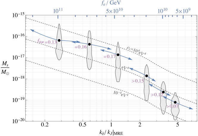
Figure 4: The mass distribution of axion stars at the final simulation times for different initial conditions, with $k_{\delta}$ the peak of the initial density power spectrum. The black dots show $\bar{M}_{s}$ defined in eq. (15); this is a weighted average that gives the typical mass of the axion stars that contain the majority of the axions that are bound in stars. The grey shapes show the distribution of axion star masses $M_{s}$, with the width of these regions proportional to $d\log n_{s}/d\log M_{s}$ where $n_{s}$ is the number density of axion stars (the area of each shape is normalised to a common, arbitrary, value). On the upper axis we indicate the axion decay constants $f_{a}$ corresponding to the different initial conditions, with the blue error bars indicating the uncertainty in relating $f_{a}$ and $k_{\delta}$. The tilt of these curves shows the resulting uncertainty in $M_{s}/M_{\odot}$ (arising because the relation between the axion star masses and $M_{\odot}$ depends on $f_{a}$). The dashed lines are contours of the corresponding central densities of the axion stars $\rho_{s}$. We also give the fraction of axions bound in axion stars at the end of the simulations, $f_{\rm star}$, which for initial $\left.k_{\delta}/k_{J}\right|_{\rm MRE}\gtrsim 2$ is still increasing.

We also show the distribution of axion star masses, $d\log n_{s}/d\log M$ where $n_{s}$ is the number density of axion stars. These results are plotted for each initial $k_{\delta}$, and related to a corresponding $f_{a}$ via Figure 2. The blue curves with arrows show the uncertainty in $f_{a}$, which is estimated from the upper and lower edges of the red band in Figure 2. Numerical simulations give the axion star masses in terms of $M_{J,{\rm MRE}}$, and the relation between this and $M_{\odot}$, given below eq. (14), depends on the value of $f_{a}$. Consequently the uncertainties in $f_{a}$ lead to overall uncertainties in $\bar{M}_{s}/M_{\odot}$ and the mass distribution, which are indicated by the vertical displacement along the blue curves. Contours of fixed $\rho_{s}$ are also plotted, obtained from eq. (13) (because the mass-central density relation of the stars that form is close to that of isolated stars). Larger initial $k_{\delta}$, corresponding to smaller $f_{a}$, leads to stars with smaller typical central densities because these form later.

By the end of the simulations $\bar{M}_{s}$ has reached an approximately constant value for initial $\left.k_{\delta}/k_{J}\right|_{\rm MRE}\leq 2.4$, consistent with $f_{\rm star}$ saturating, but $\bar{M}_{s}$ is still decreasing for larger initial $k_{\delta}$, see Figure 18 in Appendix C.3. Meanwhile, the distribution $dn/d\log M_{s}$ is still evolving at the final simulation time for all initial conditions, with axion stars of increasingly small mass continuing to form. Mergers between relatively heavy axion stars are quite rare, with only $\sim 10\%$ of the stars with mass larger than $\bar{M}_{s}/2$ having merged with another similarly heavy star prior to the end of the simulations (meanwhile, mergers between heavy and light stars are more common). We discuss the evolution of axion stars after formation further in Section 5, using analytic estimates, and leave a full numerical analysis to future work.

Note that for even larger values of $k_{\delta}/k_{J}|_{\rm MRE}$ (for which we do not have simulation results) stars will be formed even later and in smaller number, because in this case structures at $k<k_{J}$ (miniclusters) will form first and wash out smaller scale fluctuations via virialization. This is the situation for generic post-inflationary ALP dark matter (for which $k_{p}(T_{\star})\gtrsim 10H_{\star}$) and also for QCD axions with larger values of the domain wall number ($N_{\rm DW}$) if the emission from strings dominates, which leads to axion decay constants at least a factor of $N_{\rm DW}$ smaller than for the $N_{\rm DW}=1$ case that we focus on [33].

Finally, we discuss the caveats and uncertainties associated to our results. We have checked that systematic uncertainties from the lattice resolution and finite time-step are negligible compared to the other uncertainties. The finite box size introduces an uncertainty of less than 20% on $f_{\rm star}$ and $\bar{M}_{s}$, dominantly due to the shape of the initial $\mathcal{P}_{\delta}$ being slightly deformed from the infinite volume limit. Analysis of these systematical errors is provided in Appendix C.1. There is also an uncertainty associated to the definition of an axion star. Demanding that a clump’s density profile agrees with the axion star prediction to within a factor of $1.5$ rather than $2$ at $r=\lambda_{J}(\rho_{s})/4$ and $r=\lambda_{J}(\rho_{s})/2$ changes $f_{\rm star}$ and $\bar{M}_{s}$ by at most $25\%$. An alternative possible condition that $\partial_{r}\Phi$ and $\partial_{r}\Phi_{Q}$ match to within a factor $2$ at the same values of $r$ decreases $f_{\rm star}$ by at most $35\%$. A further uncertainty comes from the shape of the initial $\mathcal{P}_{\delta}$. In Appendix C.3 we show that changing the shape the peak of $\mathcal{P}_{\delta}$ by order-one amounts, keeping $k_{p}$ fixed, alters $f_{\rm star}$ and $\bar{M}$ by roughly $25\%$, which does not affect our qualitative conclusions. If $\mathcal{P}_{\delta}$ was not proportional to $k^{3}$ at $k\ll k_{p}$ this would alter the rate of hierarchical structure formation on larger spatial scales at times beyond the reach of our simulations (discussed in the next Section) but would not affect our present results. Meanwhile, the form of $\mathcal{P}_{\delta}$ at $k\gg k_{p}$ is irrelevant because the corresponding fluctuations are always prevented from collapsing by quantum pressure. As mentioned, we have neglected possible non-Gaussianities in the axion field left over from the decay of the string-wall network [56] and we have also not considered possible non-Gaussianties arising from the self-interactions at $T\sim T_{c}$. It would be interesting to investigate whether such features in the axion field could alter the number of axion stars that form, but we leave this for future work. Additionally, we reiterate that there are uncertainties in relating $f_{a}$ to the initial $k_{p}$ and $k_{\delta}$ from the earlier evolution.

5 Axion stars

As seen in the previous Sections, for any value of $f_{a}$ between $10^{10}~{}{\rm GeV}$ and $10^{11}~{}{\rm GeV}$, soon after MRE the fraction of axions contained in axion stars satisfies $0.1\lesssim f_{\rm star}\lesssim 0.2$. The actual value of $f_{a}$ mostly affects the time at which the stars form and their properties. For values of $f_{a}$ closer to $10^{11}$ GeV (corresponding to a suppressed production of axions from strings) at MRE the spectrum is slightly infrared compared to the Jeans scale and solitons form readily. At such a time the mean dark matter density is relatively large, so the axion stars in this case are comparatively dense and compact. For values of $f_{a}$ closer to $10^{10}$ GeV (associated with an enhanced production of axions from strings and favored by recent simulations [33, 34, 35, 36]) the spectrum is slightly more ultraviolet than the Jeans scale at MRE. Most solitons therefore form somewhat later, when the dark matter density has further redshifted, resulting in less compact stars. Because the initial fluctuations are on smaller comoving scales, the axion stars are also lighter in this case.

The results of the numerical simulations in Figure 4 indicate that most of the axions in stars are contained in solitons with mass given by the empirical relation

$$\bar{M}_{s}\approx 2\cdot 10^{-19}\,M_{\odot}\left(\frac{f_{a}}{10^{10}~{}{\rm GeV}}\right)^{\frac{5}{2}}\,,$$ (16)

approximately valid for $f_{a}$ between $10^{10}~{}{\rm GeV}$ and $10^{11}~{}{\rm GeV}$, with an energy density in their center

$$\bar{\rho}_{s}\approx 0.1~{}{\rm eV}^{4}\left(\frac{f_{a}}{10^{10}~{}{\rm GeV}}\right)^{4}\,,$$ (17)

and a radius

$$\bar{R}_{0.1}\approx 2.1\cdot 10^{6}~{}{\rm km}\ \left(\frac{10^{10}~{}{\rm GeV}}{f_{a}}\right)^{\frac{1}{2}}\,,$$ (18)

at which the density is a factor of ten smaller than in the center. The exact dependence on $f_{a}$ should be taken with caution given the uncertainties in relating this to the position of the peak of the density power spectrum (see e.g. Figure 4).

The axion stars therefore have a mass comparable to a mountain-size asteroid, but a radius a few times larger than the Earth-Moon distance and a density more than four orders of magnitude larger than the local dark matter density at the Sun’s location. In their gravitational ground state, the axions bound in these stars orbit with extremely low velocities

$${\bar{v}}_{b}=\frac{k_{J}(\bar{\rho}_{s})}{m}\approx 6\cdot 10^{-13}\left(\frac{f_{a}}{10^{10}~{}{\rm GeV}}\right)^{\frac{3}{2}}\sim{\rm mm/s}\,.$$ (19)

Axion stars with masses smaller than $\bar{M}_{s}$ continue to form at later times. These lighter and less dense solitons eventually dominate the number density of stars, but they remain a sub-dominant component of the dark matter energy density in stars (see e.g. Figure 17 right in Appendix C.3). Being less compact they might be more prone to tidal disruption during the subsequent evolution.

Such a large population of axion stars could have important phenomenological consequences. It is therefore crucial to understand whether they survive the cosmological evolution and what their abundance and properties would be today. Given the large hierarchies of scales involved, tracking the full evolution from matter-radiation equality until the present day is a challenging task that merits a dedicated study and is beyond the scope of our present work. We limit ourselves here to some educated estimates based on simple arguments and existing results in the literature to demonstrate the potentially interesting implications and to motivate a more systematic and precise analysis (e.g. we neglect wave effects in destruction processes [69, 70]). Several aspects of this discussion are in common with that of vector dark matter stars in ref. [51], while detailed studies for miniclusters can be found in [71, 72, 73, 74] (see also refs. [75, 76] for related analysis).

Probably the most threatening processes that could deplete our primordial axion star population are gravitational tidal disruptions among axion stars, with larger dark matter halos or with compact astrophysical objects. To estimate the importance of such events it is useful to recall that the critical distance $d_{c}$ for tidal disruption of a gravitationally bound object of mass $M_{1}$ and size $R_{1}$ (with escape velocity $v_{1}=\sqrt{2GM_{1}/R_{1}}$) off the gravitation potential of a second object of mass $M_{2}$ passing with relative velocity $v_{r}$ is given by the relation

$$\frac{d_{c}^{2}}{R_{1}^{2}}\simeq\frac{v_{1}}{v_{r}}\frac{M_{2}}{M_{1}}\,.$$ (20)

From this it follows that:

1. Two axion stars of equal masses $M_{1}=M_{2}$ can disrupt each other (i.e. $d_{c}\gtrsim R_{1}$) only if $v_{r}\lesssim v_{1}$, i.e. they are gravitationally bound to one another and they merge. This agrees with ref. [77], which finds from numerical simulations that solitons colliding with relative velocity less then the escape velocity merge into a larger star, while solitons colliding with higher velocities pass through each other basically unaffected.

2. When two axion stars of different mass (say $M_{2}>M_{1}$) get close enough, the heavier one is never disrupted while the lighter one is disrupted if $M_{2}\gtrsim M_{1}(v_{r}b^{2})/(v_{1}R_{1}^{2})$, where $b$ is the impact parameter (obtained by requiring $b\lesssim d_{c}$). Note that, as soon as larger clusters of stars form, the typical relative velocities among stars grow rapidly, hence a large hierarchy in masses is required for the less dense stars to be disrupted (typical values for $v_{r}/v_{1}$ in our galactic halo today are ${\cal O}(10^{10})$).

3. An axion star is not disrupted by other dark matter halos (such as miniclusters) if the latter are less dense than the axion star. This is indeed the typical situation in our case given that the axion stars are the first objects to form, at the locations of highest dark matter over-density. Non-solitonic halos formed at matter-radiation equality and later, while larger and more massive, are less dense. A possible caveat however is that the profiles produced during structure formation tend to develop an NFW shape with higher densities in the core, which could affect this conclusion; we discuss this further below.

4. Miniclusters are never disrupted by axion stars, passing outside them, whose mass is less than the total minicluster mass, which is also typically the case.

5. For an axion star passing in the vicinity of another compact object, such as an astrophysical star or a black hole, eq. (20) can be rewritten more conveniently using eqs. (12-13) as

   $$\frac{d_{c}^{2}}{R_{1}^{2}}\simeq\frac{GM_{2}m}{v_{r}}\qquad{\rm or}\qquad d_{c}^{2}\simeq\frac{\sqrt{G}M_{2}}{v_{r}\sqrt{\rho_{s}}}\,,$$ (21)

   where $m$ is the axion mass and $\rho_{s}$ is the axion star’s central density.

From these considerations we deduce the following evolution. After the first axion stars (which contain most of the axions that are in stars) form around matter-radiation equality, hierarchical structure formation starts. Nearby solitons begin falling into the gravitational potential of larger and larger local overdensities, accelerating toward each other and virializing into larger and larger structures. We expect that a sub-dominant portion of the initial axion star population might merge (in particular those stars that by chance are formed close enough that their relative velocity remains small when they approach each other) while the majority virializes. At this time, possible encounters among stars become irrelevant. Such a picture is compatible with what is observed in numerical simulations, where just a few stars are seen merging, although the time extent of the simulations is limited. Merging could still remain relevant for less dense axion stars, because for them this effect switches off later, when the virial velocities of structure grows above the axion stars’ mass ratios. We might therefore expect a change in the tail of the mass distribution function during hierarchical structure formation.

Because the axion stars that contain most of the dark matter (those with mass $\bar{M}_{s}$) are the most compact dark matter objects, they will not be disrupted by other dark matter halos. Indeed from the previous considerations this is probably true even for most of the rest of the axion star population. Moreover, from the estimates above, it is plausible that at least part of the fuzzy halos hosting the axion stars might also survive the hierarchical structure formation phase.

As bigger dark matter structures form, new axion stars could be created through gravitational relaxation [57]. These solitons, appearing later in the evolution, are expected to grow more massive and compact than our bulk axion star population, although they will necessarily be much rarer. It is plausible that the two different populations coexist.

During structure formation larger and larger dark matter halos develop with possibly denser cores. A virialized axion star at distance $R$ from the center of such a halo will feel a gravitational mass $M(R)=\int d^{3}x\rho(|\mathbf{x}|<R)$. Using eq. (21), tidal disruption will happen only for those stars whose central density satisfies $\rho_{s}\lesssim M(R)/R^{3}$, which is equivalent to $\rho_{s}<\rho(R)$ if the integral defining $M(R)$ is dominated by the region at $|\mathbf{x}|\simeq R$, as in the case of NFW profile (neglecting baryons, the inner NFW profiles follow the scaling $\rho(r)r=\,$const). At our position, $R\simeq 8.3$ kpc, in the Milky Way the local dark matter energy density is more than four orders of magnitude smaller than those of eq. (17), which means that this effect should not be a problem for average axion stars in typical dark matter halos. On the contrary, smaller mass axion stars are much less dense ($\rho_{s}\propto M_{s}^{4}$) so the low mass population of the axion star distribution could easily be affected. Similar conclusions follow if instead of using eq. (21) we compare the tidal force from the halo core with the gravitational force in the axion star or if we include the effects of baryons and black holes in the galactic bulge, at least for our galaxy.

Provided the arguments above are correct, we need only to worry about possible encounters between axion stars and astrophysical compact objects. Here we focus on such events within the Milky Way. Consider a typical axion star with mass $\bar{M}_{s}$ gravitationally bound in the Milky Way halo. The probability for it to be tidally disrupted by a close encounter with an astrophysical object, in particular a star, with average mass $M_{\star}$ during a crossing of the galactic disk is $P_{\times}=\sigma_{t}n_{\star}$, where $\sigma_{t}$ is the cross section for tidal disruption off an astrophysical star and $n_{\star}$ is the number density of stars per unit area on the disk. The former can be estimated simply from eq. (21)

$$\sigma_{t}=\pi d_{c}^{2}=\pi\frac{\sqrt{G}M_{\star}}{v_{r}\sqrt{\,\bar{\rho}_{s}}}\,,$$ (22)

where $v_{r}$ is now the virial velocity ${\cal O}(10^{-3})$. The latter is meanwhile given by $n_{\star}=\Sigma/M_{\star}$, where $\Sigma$ is the superficial density of stars on the galactic disk. Therefore the probability of disruption for a typical axion star crossing the galactic disk in the proximity of the Sun, where $\Sigma\simeq 50\,M_{\odot}/$pc² [78, 79], is

$$P_{\times}=\pi\frac{\sqrt{G}\,\Sigma}{v_{r}\sqrt{\,\bar{\rho}_{s}}}=6\cdot 10^{-4}\left(\frac{{\rm eV}^{4}}{\bar{\rho}_{s}}\right)^{\frac{1}{2}}\left(\frac{\Sigma}{50\,M_{\odot}/{\rm pc}^{2}}\right)\,.$$ (23)

This probability should be multiplied by the number of revolutions around the galaxy between formation and today. For low eccentricity orbits the revolution time is $T_{\rm rev.}\sim 2\pi d_{\odot}/v_{r}$ (where $d_{\odot}\simeq 8.3~{}$kpc is the distance of the Sun from the center of the galaxy), but for typical dark matter eccentricities in the halo, $e\simeq 0.9$ [80], $T_{\rm rev.}$ can be an order of magnitude larger. The average number of revolutions until today is therefore $N_{\rm rev.}\simeq{\cal O}(100)(1-e)$. The fraction of axion stars crossing the galactic disk at the Sun’s location that are tidally disrupted is therefore expected to be small with $P_{\times}N_{\rm rev.}\sim 10^{-2}\div 10^{-1}$.

We also note that the galactic dark matter halo extends much further from the center of the galaxy than the baryonic disk does, so most of the axion stars have larger orbits, with even smaller disruption probabilities, than in the estimates above. Only the tiny fraction of axion stars with very large eccentricities, again constituting a small fraction of the population, will pass close enough to the center of the galaxy (where the number density of astrophysical objects is large) to be destroyed.

We are therefore led to assume that most of the axion stars with mass of order $\bar{M}$ formed at MRE survive until today, maintaining similar properties, and in particular that this is the case for stars with orbits in the Milky Way halo comparable or larger than that of our solar system.

The local number density of such axion stars is $n_{s}=f_{\rm star}\rho_{\rm DM}^{\rm loc}/\bar{M}_{s}$, where $\rho_{\rm DM}^{\rm loc}$ is the average local dark matter density, which we take to be $0.4~{}{\rm GeV}/{\rm cm}^{3}$. Consequently, the average distance between two axion stars is

$$n_{s}^{-1/3}=1.4\cdot 10^{8}\,{\rm km}\left(\frac{\bar{M}_{s}}{10^{-19}\,M_{\odot}}\right)^{\frac{1}{3}}\left(\frac{0.1}{f_{\rm star}}\right)^{\frac{1}{3}}\,,$$ (24)

i.e. typically there are four axion stars within one astronomical unit of us and $10^{5}$ in the solar system at any given time! Consequently, the rate at which solitons pass through Earth might be non-negligible. Indeed we can estimate the average waiting time on Earth for an encounter with an axion star of mass $M_{s}$ to be $\tau_{\oplus}=1/(\sigma_{\oplus}n_{s}v_{r})$, where $\sigma_{\oplus}=\pi R^{2}$ is the geometric cross section for encountering an axion star at distance $\leq R$ from its center and $v_{r}$ the virial velocity. Substituting the relevant values we get

$$\tau_{\oplus}=5~{}{\rm yrs}\left(\frac{R_{0.1}}{R}\right)^{2}\left(\frac{0.1}{f_{\rm star}}\right)\left(\frac{\bar{M}_{s}}{10^{-19}M_{\odot}}\right)^{3}\left(\frac{10^{10}~{}{\rm GeV}}{f_{a}}\right)^{4}\,,$$ (25)

which, substituting $\bar{M}_{s}$ from eq. (16), suggests that for low $f_{a}$ the axion stars’ encounters with Earth might be interestingly frequent! Such encounters would last for an interval

$$\Delta t\simeq\frac{2R_{0.1}}{v_{r}}\sqrt{1-\frac{R^{2}}{R_{0.1}^{2}}}=8~{}{\rm hrs}\left(\frac{10^{-19}M_{\odot}}{\bar{M}_{s}}\right)\left(\frac{f_{a}}{10^{10}~{}{\rm GeV}}\right)^{2}\sqrt{1-\frac{R^{2}}{R_{0.1}^{2}}}\,,$$ (26)

which can be long compared to timescales relevant to experiments. One may wonder whether axion stars would be tidally disrupted by the Earth or the Sun before reaching the surface of the Earth. In fact an axion star passing through the Earth will be disrupted, however this would happen much after the star has left the Earth.

Given that the dark matter density inside the axion stars could be more than four orders of magnitude larger than the average local one, for axion dark matter experiments looking in this mass range, such as those in refs. [81, 82], a broadband strategy might be more competitive than a resonant one. Note also that there could be many more stars with smaller density but bigger cross sections flying around. While their survival probability is less certain, their presence could have important implications for experiments: if at least part of this population survives until today it could completely alter expectations for the local dark matter density observed on Earth, which would fluctuate continuously by orders of magnitudes over time scales of order days or more. The streams resulting from the destruction of such stars could also lead to interesting features in the dark matter density [83, 84].

6 Conclusion

To summarize, we find that in the axion post-inflationary scenario the dark matter power spectrum resulting from the decay of topological defects is peaked near the quantum Jeans scale at matter-radiation equality, almost independently of the uncertainties in the precise value of the QCD axion mass that fits the observed dark matter abundance, at least provided $f_{a}\gtrsim 10^{10}~{}{\rm GeV}$ (see Figure 2). This coincidence enhances the number of axion stars that form around the time of matter-radiation equality. Numerical simulations confirm this expectation showing that 10 to 20% of the total dark matter axions end up gravitationally bound in solitonic cores, which are surrounded by less dense halos containing a larger fraction of the remaining dark matter particles (see Figure 3). Estimates suggest that a sizable fraction of this primordial axion star population survives to the present day in our galaxy. The axion stars have a much larger density than the average local dark matter density in the neighborhood of the Sun (around four orders of magnitude for $f_{a}\simeq 10^{10}$ GeV, see eq. (17)) and one could pass though a detector on Earth every few years, see eq. (25).

There are several important directions for future work. As mentioned, perhaps the most urgent of these is a dedicated study of the evolution of the axion stars after MRE. To this end, it would be useful to carry out simulations from MRE until later times than we have been able to. This would require a greater separation between the box size and the lattice spacing, a challenge that is well suited to adaptive mesh refinement, as implemented in refs. [85, 86]. Such simulations would allow the first stages of hierarchical structure formation, as the axion stars cluster into larger objects, to be studied and precise statistics about possible soliton disruption or mergers to be obtained. It would also be interesting to analyze the evolution of the axion stars within their surrounding fuzzy-halos, for example to determine whether the stars increase in mass due to accretion or evolve towards the core-halo relation proposed in ref. [87], and to study the decay of their quasinormal modes. The dynamics of the axion stars at even later times, within the much larger halos from adiabatic perturbations, and their probability of survival in the Earth’s local environment are also critical.

Numerous possible signals of axion clumps in the post-inflationary scenario have been proposed and analyzed in the literature, and reanalysing these in light of our results would be worthwhile. Gravitational signals can arise from lensing effects [88], although in the case of femtolensing (which is the most relevant process for the axion stars themselves given the masses that we find) the sensitivity is weak due to finite source size and wave optics effects [89]. Heavier “mini-halos” from the IR part of the density power spectrum could lead to micro-lensing events [18, 19]. Particularly promising is caustic microlensing [90], which might be sensitive to axion mini-halos with masses as small as $10^{-15}M_{\odot}$. Gravitational signals of dark matter clumps inside the solar system have also recently been considered [91, 92, 93], including for clumps in the mass range we expect for axion stars; these are interesting given our prediction of a large number of axion stars. There are also possible signals arising from the solitonic nature of the axion stars (which have previously been studied assuming stars form by condensation inside miniclusters) that typically rely on the axion-photon coupling. There has been extensive work on signals from collisions between axion stars and neutron stars [94, 95, 96, 97, 98, 99, 100] or main sequence stars [101]. Other ideas include axion stars converting to photons in the Milky Way [102], monochromatic photon signals from collapsing axion stars [103, 104], and radio emission from axion stars [105]. Finally, we reiterate that a detailed analysis of the implications of our results for direct detection experiments would certainly be valuable.

Appendix A Details of the self-interactions

A.1 The non-relativistic axion field

After the string-wall network collapses at $T\simeq T_{\star}$, the axion field $\phi$ follows the Klein–Gordon equation of motion with potential $V=\frac{1}{2}m^{2}\phi^{2}-\frac{1}{4!}\lambda\phi^{4}+\dots$, with temperature-dependent (i.e. time-dependent) mass $m$ and quartic coupling $\lambda$.

In the non-relativistic limit, it is convenient to rewrite the equation of motion of $\phi$ in terms of $\psi$ defined by eq. (8) in the main text, which leads to eq. (9). The gravitational potential $\Phi$ satisfies

$$\nabla^{2}\Phi=\frac{4\pi G}{a^{3}}\frac{m}{m_{0}}\left(|\psi|^{2}-\overline{|\psi|^{2}}\right)\,,$$ (27)

where, as in the main text, an over-line denotes the spatial average ($m_{0}$ is the zero-temperature axion mass). $\Phi$ has a negligible effect in the axion field’s equation of motion deep in radiation domination, including when $T\gtrsim T_{c}$. Still considering the non-relativistic limit, the axion energy density and number density are given by, respectively,

$$\rho=\frac{1}{2}\dot{\phi}^{2}+\frac{1}{2}m^{2}\phi^{2}=\frac{m}{m_{0}}\frac{|\psi|^{2}}{a^{3}}\,,\qquad\qquad n=\frac{\rho}{m}=\frac{|\psi|^{2}}{m_{0}a^{3}}\,.$$ (28)

The spatially averaged comoving number density, $\bar{n}a^{3}=\overline{|\psi|^{2}}/m_{0}$, is conserved even when $m$ is temperature-dependent, while the average of $\rho a^{3}$ is not conserved and instead increases while $m$ is growing.

At $T\gtrsim T_{c}$, the axion mass is temperature-dependent. We model this dependence as

$$\frac{m}{m_{0}}=\left[1+\left(\frac{T}{T_{c}}\right)^{\frac{\alpha}{2r}}\right]^{-r}~{},$$ (29)

with $\alpha\simeq 8$ and $r\simeq 0.4$ providing reasonable fits to lattice data [54], where we set $T_{c}=155\,{\rm MeV}$ (note that $m^{2}\propto T^{-\alpha}$ for $T\gg T_{c}$). Although the quartic coupling at $T>T_{c}$ is not well determined from current lattice results, we assume that it takes the form

$$\lambda=c_{0}\left[1+c_{0}^{\frac{1}{2r}}\left(\frac{T}{T_{c}}\right)^{\frac{\alpha}{2r}}\right]^{-2r}\frac{m^{2}_{0}}{f_{a}^{2}}\,,$$ (30)

where $c_{0}=0.35$ and, as before, $\alpha\simeq 8$ and $r\simeq 0.4$. Eq. (30) is such that $\lambda=c(T)m^{2}/f_{a}^{2}$ with $c(T)$ interpolating between the zero temperature value from chiral perturbation theory, $c(T\ll T_{c})\simeq c_{0}$ [106], and the dilute instanton gas prediction $c(T\gg T_{c})=1$.

With the preceding axion mass temperature dependence at $T\gg T_{c}$ (and using that the effective number of relativistic degrees of freedom at $T=T_{\star}$ is $g_{\star}\simeq 60$), we obtain

$$\frac{T_{\star}}{T_{c}}\simeq 20\left(\frac{10^{10}~{}{\rm GeV}}{f_{a}}\right)^{1/6}~{}.$$ (31)

Provided that, as is expected, the string-wall network is destroyed when $m$ is roughly of order $H$, all of the strings and domain walls are destroyed soon after $T=T_{\star}$ with only a weak dependence on the particular value of $m/H$ at which the destruction happens because of the fast growth of the axion mass (simulation results find that for $\log(m_{r}/H_{\star})\simeq 6$ no strings remain after $T\simeq T_{\star}/2$ [56]).

Freely-propagating modes of momentum $k_{p}$ become non-relativistic at approximately $a/a_{\star}=\left(\left.k_{p}/H_{\star}\right|_{T=T_{\star}}\right)^{1/(\alpha/2+1)}$. Therefore, in the absence of a non-linear transient, basically all modes of interest are non-relativistic by $a/a_{\star}\simeq 2$ assuming $k_{p}(T_{\star})\sim 10H_{\star}$. The situation is more complicated in the case of a sizable non-linear transient as the axion field becomes non-relativistic, as occurs for $f_{a}\lesssim 5\times 10^{10}~{}{\rm GeV}$. In this case, the temperature of the Universe when the axion field is first non-relativistic is in the range $T_{\ell}=T_{\star}/3$ (for $f_{a}\simeq 10^{10}~{}{\rm GeV}$) and $T_{\ell}=T_{\star}/2$ (for $f_{a}\simeq 5\times 10^{10}~{}{\rm GeV}$). The axion energy spectrum is modified by such a transient, in particular its peak is shifted close to the value of the axion mass at the time when $T=T_{\ell}$. Full expressions for $T_{\ell}$ and $k_{p}$ after this transient, simulations confirming these dynamics, and fits of the order-one coefficients that appear in the analytic formulae can be found in ref. [33]. Here we simply note that (with the values of the numerical coefficients obtained in [33]) $k_{p}(T_{\ell})$ corresponds to

$$\left.\frac{k_{p}}{k_{J}}\right|_{\rm MRE}\simeq 0.4\left(\frac{10^{10}~{}{\rm GeV}}{f_{a}}\right)^{1/2}~{},$$ (32)

which is the red line in Figure 2. For sufficiently large $f_{a}$ such a non-linear transient is absent; the simulations results in [33] show that the critical value of $f_{a}$ above which there at most a minor effect on the axion spectrum is approximately $5\times 10^{10}~{}{\rm GeV}$.

We also note that, as discussed in Footnote 2, some oscillons will form during the decay of the string-wall network and will persist after $T=T_{\ell}$, however these small objects do not affect the dynamics on the larger scales.

A.2 Analytic analysis

As discussed in Section 3, self-interactions drive the peak of the axion energy spectrum towards the UV. The rate at which this occurs depends on the relative size of the gradient and self-interaction energy densities in the Hamiltonian.

Neglecting gravity, in the non-relativistic regime the equation of motion of the axion field, eq. (9), can be written in terms of its Fourier transform $\psi_{\bm{k}}(t)$ defined by $\psi(t,{\bm{x}})\!=\!\int\!\!\frac{d^{3}k}{(2\pi)^{3}}\psi_{\bm{k}}(t)e^{-i{\bm{k}}.{\bm{x}}}$ as

$$i\partial_{t}\psi_{\bm{k}}=\frac{k^{2}}{2m}\psi_{\bm{k}}-\frac{\lambda}{8m^{3}}\int\frac{d^{3}{p}\,d^{3}{q}\,d^{3}{l}}{(2\pi)^{9}}\psi_{\bm{p}}^{*}\psi_{\bm{q}}\psi_{\bm{l}}(2\pi)^{3}\delta^{(3)}({\bm{k}}+{\bm{p}}-{\bm{q}}-{\bm{l}})~{},$$ (33)

which holds regardless of the relative sizes of the gradient and self-interaction terms in the Hamiltonian.

For $(\nabla\phi)^{2}\gtrsim\lambda\phi^{4}$ the non-relativistic axion momentum modes have dispersion relation $\omega_{\bm{k}}\simeq k^{2}/(2m)$ (up to small corrections from the self-interactions) and the system is well described by kinetic theory [30, 57, 107, 108, 109]. In this limit eq. (33) implies (see e.g. [110] for a derivation)

$$\partial_{t}f_{\bm{k}}=\frac{\lambda^{2}}{32m^{4}}\int\frac{d^{3}{p}\,d^{3}{q}\,d^{3}{l}}{(2\pi)^{9}}(2\pi)^{4}\delta^{(4)}(k+p-q-l)\left((f_{\bm{k}}+f_{\bm{p}})f_{\bm{q}}f_{\bm{l}}-(f_{\bm{q}}+f_{\bm{l}})f_{\bm{k}}f_{\bm{p}}\right)~{},$$ (34)

where the mode occupations $f_{\bm{k}}\equiv|\psi_{\bm{k}}|^{2}/(mV)$ (with $V$ the system volume) such that $\bar{\rho}=m\int d^{3}k/(2\pi)^{3}f_{\bm{k}}$, and the free dispersion relation is assumed in the energy part of the delta function. Using that the typical momentum and energy scales are $k_{p}$ and $k_{p}^{2}/2m$ in eq. (34), and that $f_{\bm{k}}/(2\pi)^{3}\sim\bar{\rho}/(mk_{p}^{3})$, this leads to the estimate of the thermalisation rate given in the main text

$$\tau_{\rm therm}=\left(\frac{1}{f_{\bm{k}}}\frac{\partial f_{\bm{k}}}{\partial t}\right)^{-1}\simeq 64\frac{m^{5}k_{p}^{2}}{\lambda^{2}\bar{\rho}^{2}}~{},$$ (35)

(note that the numerical coefficient on the right hand side of eq. (35) is not sharply determined). Using the approximate relation $\lambda(T)\simeq m^{2}(T)/f_{a}^{2}$ and that the axion number density is $n=\rho/m$ we have

$$\tau_{\rm therm}H\simeq 64\frac{f_{a}^{4}k_{p}^{2}}{{n}^{2}(T_{\star}/T)^{6}}\frac{m_{\star}}{m}\left(\frac{T}{T_{\star}}\right)^{-4}~{},$$ (36)

which is valid both for the QCD axion and an ALP. The denominator in the first fraction is the axion number density redshifted back to $T_{\star}$ assuming comoving number density conservation (this will not coincide with the true axion number density at $T_{\star}$ if there is a first non-linear transient as the axion field becomes non-relativistic). For an ALP with a temperature-independent mass eq. (36) simplifies to eq. (4) in the main text. As discussed in Section 3, such a particle satisfies $(\nabla\phi)^{2}\gtrsim\lambda\phi^{4}$ for all $T<T_{\star}$ so $\tau_{\rm therm}$ is the relevant timescale for self-interactions, and moreover $\tau_{\rm therm}H\gtrsim 1$ for all $T<T_{\star}$.

Conversely, in the regime $(\nabla\phi)^{2}\ll\lambda\phi^{4}$ the gradient term in the axion’s equation of motion, eq. (9), is irrelevant compared to the self-interactions (this is similar to the situation soon after preheating, as occurs in some theories of cosmic inflation, analyzed in ref. [111]). As mentioned in the main text, in this limit the only timescale in the axion field’s equation of motion is

$$\tau_{v}=\frac{8m}{\lambda\phi^{2}}\simeq\frac{8f_{a}^{2}}{n}~{},$$ (37)

which is therefore expected to set the time for the axion spectrum to change by an order-one amount.

For the QCD axion at $T_{c}\ll T<T_{\ell}$ (where $T_{\ell}<T_{\star}$ is the temperature at which the axion field is non-relativistic after the first transient), we have $m\simeq m_{\star}(T/T_{\star})^{-4}$, $\lambda\sim m^{2}/f_{a}^{2}$ and the comoving axion number density is conserved. This leads to

$$\tau_{v}H\simeq\left(\frac{m_{\star}f_{a}^{2}}{n(T_{\star}/T)^{3}}\right)\left(\frac{T_{\star}}{T}\right)~{}.$$ (38)

Using $(T_{c}/T_{\star})\simeq(f_{a}/M_{p})^{1/6}$, and $m_{\star}/m_{0}\simeq(f_{a}/M_{p})^{2/3}$, $m_{0}\sim T_{c}^{2}/f_{a}$ we obtain

$$\tau_{v}H\sim\left(\frac{f_{a}}{M_{\rm Pl}}\right)\left(\frac{T_{c}}{T_{\rm MRE}}\right)\left(\frac{T_{c}}{T}\right)~{}.$$ (39)

Repeating this calculation including numerical factors leads to eq. (6) in the main text. We see that the axion self-interactions are relevant when the comoving axion number density is larger than the naive contribution from domain wall decay $n(T_{\star}/T)^{3}\simeq m_{\star}f_{a}^{2}$, corresponding to $f_{a}\lesssim 5\times 10^{10}~{}{\rm GeV}$. This is indeed the case if the number of strings per Hubble patch $\xi\sim 10$ at $T\simeq T_{\star}$ and a scale-invariant or IR dominated emission spectrum, as is strongly suggested by simulation results. We also note that the thermalisation timescale valid instead for $(\nabla\phi)^{2}\gtrsim\lambda\phi^{4}$ is related to $\tau_{v}$ by

$$\tau_{\rm therm}=\tau_{v}\left(\frac{k_{p}}{k_{v}}\right)^{2}~{},$$ (40)

where $k_{v}\equiv\sqrt{\lambda{\phi^{2}}}$ is the critical momentum such that $(\nabla\phi)^{2}\simeq\lambda\phi^{4}$, as described below eq. (6). As a result, the timescale $\tau_{v}$ connects to $\tau_{\rm therm}$ continuously as $k_{p}$ increases towards $k_{v}$ and the rate at which energy moves to the UV slows down for $k_{p}\gtrsim k_{v}$. Denoting comoving momenta $\tilde{k}\equiv k(a/a_{\star})$, a straightforward calculation gives

$$\tilde{k}_{v}(T)\sim 700\tilde{k}_{\star}\left(\frac{T_{c}}{T}\right)^{3/2}\left(\frac{10^{10}\,{\rm GeV}}{f_{a}}\right)^{5/6}~{},$$ (41)

where $k_{\star}\equiv H_{\star}$, for $T\gg T_{c}$ (this breaks down around $T\simeq T_{c}$ when the temperature dependence of the axion mass changes). Assuming that $f_{a}\lesssim 5\times 10^{10}~{}{\rm GeV}$ such that a first non-linear transient occurs, at $T=T_{\ell}\sim 5T_{c}$ (when the axion field becomes non-relativistic) the peak of the axion spectrum is at $\tilde{k}_{p}(T_{\ell})\simeq 200\tilde{k}_{\star}\left(10^{10}~{}{\rm GeV}/f_{a}\right)^{5/6}$ (obtained from eq. (32)). Therefore, at $T=T_{\ell}$ the spectrum peak is typically a factor of a few larger than $\tilde{k}_{v}(T_{\ell})$. From eq. (41), $\tilde{k}_{v}$ rapidly increases as the temperature drops below $T_{\ell}$ and, if the field’s evolution were not affected by the self-interactions, the regime $k_{p}\ll k_{v}$ would quickly be reached (as discussed in Section 3, see also Figure 5 below).

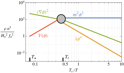
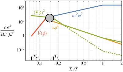
Figure 5: Left: The schematic evolution of different contributions to the total energy density of an axion-like-particle with a temperature-independent mass as a function of the temperature of the Universe $T$ (relative to $T_{c}=155~{}{\rm MeV}$). We set the axion mass such that $H=m$ at $T=T_{\star}\simeq 2~{}{\rm GeV}$. Immediately after $T=T_{\star}$ the axion field is relativistic and has field amplitude larger than $f_{a}$. Once the potential energy $V(\phi)$ is comparable to the gradient energy, at $T=T_{\ell}$, there is a non-linear transient, indicated by the grey circle. Subsequently, at $T<T_{\ell}$, the axion field is non-relativistic with the mass contribution to the energy density dominant and the gradient energy larger than the quartic self-interaction. Right: The analogous plot for the QCD axion. There is again a non-linear transient when $(\nabla\phi)^{2}\simeq V(\phi)$. Subsequently, the self-interaction energy $\lambda\phi^{4}$ decreases slower than the gradient energy $(\nabla\phi)^{2}$. In the absence of scattering processes mediated by the self-interactions, the quartic contribution to the energy density would exceed the gradient energy density soon after $T=T_{\star}$ (dashed line). However, self-interactions transfer energy to high momentum modes in such a way that $\lambda\phi^{4}\sim(\nabla\phi)^{2}$ is maintained (solid lines). This regime continues until $T\simeq T_{c}$ when the hierarchy $\lambda\phi^{4}\ll(\nabla\phi)^{2}$, as in the axion-like-particle case, is restored.

The preceding expressions for $\tau_{\rm therm}$ and $\tau_{v}$, in combination with the scalings of the gradient and self-interaction energy densities, result in the effects described in Section 3. These are illustrated in Figure 5, in which we plot the evolution of the mass, gradient and self-interaction energy densities for an ALP with constant mass (left) and the QCD axion (right). Soon after $T=T_{\star}$, for both an ALP and a QCD axion, the field amplitude is much larger than $f_{a}$, the gradient energy dominates the potential energy (bounded from above as $V(\phi)\lesssim m^{2}f_{a}^{2}$) and the axion evolves as a free relativistic field [33, 112]. Once the gradient energy has decreased sufficiently that $(\nabla\phi)^{2}\simeq V(\phi)$, the axion potential becomes relevant and there is a non-linear transient in which both $(\nabla\phi)^{2}$ and $V(\phi)$ change non-trivially. After this non-linear transient, the axion field is non-relativistic with amplitude less than $f_{a}$. For an ALP, the field is subsequently free and the comoving energy spectrum remains fixed until MRE. Meanwhile, for a QCD axion the field is free only until $(\nabla\phi)^{2}$ and $\lambda\phi^{4}$ become of the same order as a result of the rapid increase of $V(\phi)$. At this point the self-interactions become relevant and drive the peak of the axion energy spectrum close to $k_{v}$. For $f_{a}\lesssim{\rm few}\times 10^{10}~{}{\rm GeV}$ this is maintained until $T\simeq T_{c}$.

To see the effects of the self-interactions for a QCD axion in more detail, in Figure 6 we show the temperature-evolution of $\tilde{k}_{v}$ and $\tau_{v}$ for different values of $f_{a}$. These are evaluated using the expressions of $m$ and $\lambda$ in eqs. (29) and (30). As the temperature of the Universe decreases from $T_{\star}$ to $T_{c}$, the critical comoving momentum $\tilde{k}_{v}\propto T^{-3/2}$ increases and the timescale on which self-interactions affect the spectrum increases relative to Hubble as $\tau_{v}H\propto T^{-1}$. We therefore expect $\tilde{k}_{p}$ to be roughly set by the value of $\tilde{k}_{v}$ when the self-interactions freeze out, i.e. when $\tau_{v}H\simeq 1$. As can be seen from the Figure, for $f_{a}\simeq 10^{10}~{}{\rm GeV}$, $\tau_{v}H\lesssim 1$ until $T\simeq T_{c}$ (as anticipated above) and $\tilde{k}_{v}\simeq 500\tilde{k}_{\star}$ at this time. Conversely, for $f_{a}\gtrsim{\rm few}\times 10^{10}~{}{\rm GeV}$ the non-linear interactions freeze out at $T\gtrsim T_{c}$. In the extreme case $f_{a}\gtrsim 10^{11}~{}{\rm GeV}$, $\tau_{v}H\lesssim 1$ only at $T\gtrsim 5T_{c}$ and the corresponding $\tilde{k}_{v}\sim 10\tilde{k}_{\star}$, so a much less dramatic change to the initial spectrum is expected.

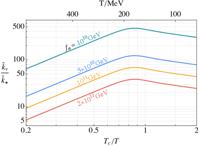
Figure 6: Left: The critical comoving momentum $\tilde{k}_{v}\equiv k_{v}(a/a_{\star})$ such that an axion field with energy spectrum sharply peaked at $k_{v}$ satisfies $(\nabla\phi)^{2}\sim\lambda\phi^{4}$ (in particular such that the contributions of these resulting terms in the axion’s equation of motion are equal). Results are shown as a function of the temperature of the Universe $T$ compared to $T_{c}=155~{}{\rm MeV}$, and for different values of $f_{a}$. Right: Comparison between the timescale $\tau_{v}=8m/(\lambda\phi^{2})$ over which the axion energy spectrum evolves while in the regime $(\nabla\phi)^{2}\ll\lambda\phi^{4}$ and the Hubble parameter $H(T)$.

A.3 Setup of simulations

We solve the equations of motion in eq. (9) in comoving coordinates on a discrete lattice using a second order pseudo-spectral algorithm as described in [113, 86], see also [57]. This algorithm (as with its sixth order version, which we find has similar efficiency) has the benefit of preserving the comoving axion number density $\bar{n}a^{3}$ to high precision as well as being fairly fast. For simplicity, we assume that the number of degrees of freedom $g_{s}$ is constant for $T_{c}\lesssim T\lesssim T_{\star}$, so that $T/T_{c}=a(T_{c})/a$. In particular, we set $g_{s}=25$, which is the value appropriate to temperature slightly above $T_{c}$ (we expect that including the full temperature dependence would have at most a minor effect on our results). Moreover, we assume the axion mass and quartic have the form in eqs. (29) and (30), with the parameter values quoted there (we have checked that changing $r$ by an order one factor and varying $\alpha$ in the range $[6,10]$ does not substantially affect the final position of the peak of the axion spectrum once the self-interactions freeze out at $T\lesssim T_{c}$).

We start cosmological simulations at the time when $T=5T_{c}$, which is a reasonable estimate of when the axion field is first non-relativistic for the $f_{a}\in[10^{10},10^{11}]~{}{\rm GeV}$ that we consider. We have checked that our results do not change substantially (compared to the uncertainties we estimate in Figure 2) if the initial $T/T_{c}$ is varied by a factor of $2$ in either direction. We fix the axion field in the initial conditions to have a Gaussian distribution with power spectrum

$$\mathcal{P}_{\dot{\phi}}(k)=m^{2}\mathcal{P}_{\phi}=\frac{\partial\rho}{\partial\log k}\propto\left(\frac{k}{k_{p}}\right)^{4}\left[1+4\left(\frac{k}{k_{p}}\right)^{\frac{5}{s}}\right]^{-s}\ ,$$ (42)

and for each $f_{a}$ we carry out simulations with different peak locations $k_{p}$. The parameter $s$ in the ansatz in eq. (42) parameterizes the shape of the spectrum. For $s\simeq 4$, the shape is a good match to that emerging from the non-linear transient as the axion field becomes non-relativistic, as occurs for $f_{a}\lesssim 5\times 10^{10}~{}{\rm GeV}$ [33]. We assume that this shape is a reasonable fit to the initial spectrum also for larger $f_{a}$ (in which case it is directly determined by the string-wall decay). The uncertainties arising from our limited knowledge of the initial spectrum are discussed in Appendix A.4.

Systematic uncertainties in our numerical simulations arise from the finite time-step, the finite box size, and the finite lattice spacing. We have tested the impact of these for each $f_{a}$ and initial $k_{p}$ (different simulation parameters are required to avoid systematic uncertainties in each case). The time-step is chosen sufficiently small that it introduces at most order $\%$ level uncertainty. We fix the box size $L$ large enough that the peak of the axion energy spectrum is well captured with $2\pi/L\lesssim k_{p}/3$ (we have tested that the results are unchanged for bigger $L$). The number of lattice points that we have sufficient computing resources to evolve, $N^{3}\lesssim 512^{3}$, then limits the lattice spacing. In Figure 7 left we plot the axion energy spectrum at the final simulation time in cosmological simulations starting from the same initial conditions for different lattice spacing. The finite lattice spacing leads to an unphysical peak in the axion energy spectrum, at momentum modes within a factor of $2$ of the lattice spacing scale, forming during the evolution. As expected, the fraction of the total energy in this unphysical peak decreases as the lattice spacing is decreased. If such a peak contains more than approximately $25\%$ of the total energy or is not well-separated from the main peak, the shape and evolution of the main, physical, part of the spectrum is affected (i.e. there are significant systematic uncertainties from the finite lattice spacing). We therefore consider results from flat-space simulations only prior to too much energy reaching the lattice scale. Meanwhile for cosmological simulations we only consider initial values of $k_{p}$ such that less than approximately $25\%$ of the total energy reaches modes within a factor of 2 of the lattice spacing before the self-interactions freeze out and the spectrum reaches its final form at $T\lesssim T_{c}$.

Figure 7: Left: The comoving axion energy density spectrum at the initial (black) and final simulation times, when $T=5T_{c}$ and $T=T_{c}/2$ respectively, for $f_{a}=5\times 10^{10}~{}{\rm GeV}$ and initial $\tilde{k}_{p}\simeq 50\tilde{k}_{\star}$. To test the impact of the finite lattice spacing systematic uncertainties, we carry out simulations with the same comoving box size $L$ and different comoving lattice spacing $L/N$ where $N^{3}$ is the number of lattice points. For $N^{3}\leq 256^{3}$ energy that accumulates at the lattice spacing scale affects the shape of the spectrum around its peak substantially, but for $N^{3}\geq 384^{3}$ the main part of the spectrum in approximately independent of $N$ and free of systematic errors. Right: The axion energy spectra at the initial and final simulation times, dashed and solid lines respectively, for $f_{a}=5\times 10^{10}~{}{\rm GeV}$. Results are shown for different initial shaped spectra, parameterized by $s$ in eq. (42), with all spectra having initial $\tilde{k}_{p}\simeq 50\tilde{k}_{\star}$. Order-one changes to the initial spectrum only have a relatively minor effect on the final spectrum.

A.4 Results from simulations

Flat space-time simulations

In order to confirm the validity of $\tau_{v}$ in eq. (5), we present results from simulations in flat space-time, $a=1$, with $m$ and $\lambda$ time-independent so $k_{v}$ and $\tau_{v}$ are constant (normalizing length scales to $k_{v}$ and time to $\tau_{v}$, the non-relativistic equations of motion are then independent of $\bar{|\psi|^{2}}$). In Figure 8 we show the evolution of the energy density spectrum $\frac{1}{\bar{\rho}}\frac{\partial\rho}{\partial\log k}$ as a function of time for initial $k_{p}\ll k_{v}$ (left) and for $k_{p}\simeq k_{v}$ (right); as in the main text, $\rho$ is the total axion energy density, which is dominated by the mass energy such that $\frac{\partial\rho}{\partial\log k}\propto\frac{\partial n}{\partial\log k}$ with $n$ the axion number density. In the case $k_{p}\ll k_{v}$, energy shifts to the UV on time-scale of order $\tau_{v}$, with $k_{p}$ increasing by a factor of $10$ by $t\simeq\tau_{v}$ regardless of the particular initial value of $k_{p}$ (we only plot results up to $1.5\tau_{v}$ because after this so much energy is at the lattice spacing scale that systematic uncertainties become significant). Conversely, for $k_{p}\simeq k_{v}$ there is only an order-one change in the spectrum between $t=0$ and $5\tau_{v}$. Subsequently, the spectrum is approximately constant on timescales of order $\tau_{v}$. This is consistent with the analytic scattering calculation, expected to be valid in this regime, which gives $\tau_{\rm therm}\simeq\tau_{v}(k/k_{v})^{2}$ for $k\gtrsim k_{v}$.

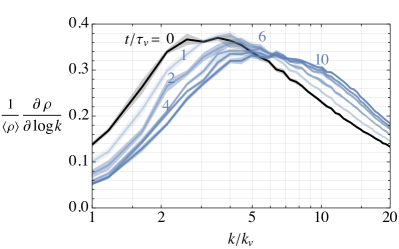
Figure 8: Left: The time-evolution of the axion energy density spectrum in flat space-time simulations with energy density spectrum initially peaked at $k_{p}\ll k_{v}$. On timescales of order $\tau_{v}$ axion self-interactions drive the energy into the UV, to momenta much larger than $k_{p}(0)$. Right: Analogous to the left plot but with initial $k_{p}\simeq k_{v}$. Between $t=0$ and $t\simeq 5\tau_{v}$ the spectrum moves slightly towards the UV, and subsequently its rate of change decreases.

As further confirmation, in Figure 9 we plot the time-evolution of the spectrum peak $k_{p}$ for different initial $k_{p}$, again in flat space-time simulations. As expected, while $k_{p}\ll k_{v}$ the axion spectrum moves towards the UV on timescales of order $\tau_{v}$. (For initial $k_{p}\ll k_{v}$, between $t=0$ and $t=\tau_{v}/2$ the shape of the spectrum changes without the location of the peak moving too much, which accounts for the plateaus in the plot at these times.) Meanwhile, for initial $k_{p}\gtrsim 3k_{v}$ the spectrum peak moves at a much slower rate.

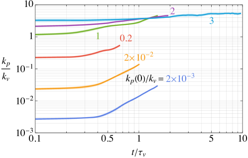
Figure 9: The time-evolution of the peak position $k_{p}$ of the axion energy density spectrum $\partial\rho/\partial\log k$ in flat space-time simulations, starting from different initial $k_{p}$ (labelled $k_{p}(0)$). Momenta are normalized relative to the critical momentum $k_{v}$ such that $(\nabla\phi)^{2}=\lambda\phi^{4}$ and times are normalized relative to $\tau_{v}=8m/(\lambda\phi^{2})$.

Cosmological simulations

Cosmological simulations of the axion field from from $T\simeq T_{\ell}$ to $T\lesssim T_{c}$ show that the energy spectrum evolves in the way expected from the analytic analysis and the flat space-time results. First, in Figure 10 we plot the energy spectrum at different $T$ for $f_{a}=10^{10}~{}{\rm GeV}$ and $f_{a}=10^{11}~{}{\rm GeV}$, with initial $k_{p}$ set to the physically expected values (from the preceding relativistic transient and from string decay for the two $f_{a}$, respectively).

Figure 10: Left: The evolution of the axion energy spectrum due to self-interactions between $T=5T_{c}$ (roughly when the field is first non-relativistic) and $T/T_{c}=1/2$ (after which spectrum is close to constant), for $f_{a}=10^{10}\,{\rm GeV}$. The initial conditions have comoving $\tilde{k}_{p}\simeq 200\tilde{k}_{\star}$, as expected after the preceding non-linear relativistic transient. The self-interactions have a substantial effect, driving $\tilde{k}_{p}$ towards the UV. Right: Analogous plot for $f_{a}=10^{11}~{}{\rm GeV}$ with initial $\tilde{k}_{p}\simeq 20\tilde{k}_{\star}$. In this case the axion self-interactions have a less dramatic impact.

For $f_{a}=10^{10}~{}{\rm GeV}$ the axion self-interactions have a substantial effect between $T=5T_{c}$ and $T\simeq T_{c}$ increasing $\tilde{k}_{p}\equiv k_{p}(a/a_{\star})$ by about a factor of $4$ and broadening the peak. The final $\tilde{k}_{p}$, once the self-interactions have frozen out, is a factor of a few larger than a naive estimate from the analytic results in Figure 6. This is consistent with the flat space results of Figure 9 in which $k_{p}$ changes by order-one amounts in times $\tau_{v}$ for $k_{p}\lesssim 5k_{v}$. Meanwhile for $f_{a}=10^{11}~{}{\rm GeV}$ the effect of the self-interactions is somewhat smaller with only, roughly, a factor of $2$ change in $\tilde{k}_{p}$. In this case, the change in the spectrum mostly takes place while $T\gtrsim 2T_{c}$ (which is consistent with our analytic expectation in Figure 6).

To obtain more general predictions, we carry out simulations with a range of initial $\tilde{k}_{p}$ for different $f_{a}$. The results are summarized in Figure 11,

Figure 11: The final position of the peak of the comoving axion energy spectrum, $\tilde{k}_{p}(t_{f})$, once the axion self-interactions have frozen out (when $T<T_{c}$) as a function of its initial position, $\tilde{k}_{p}(t_{i})$ for different $f_{a}$. The approximate $\tilde{k}_{p}(t_{i})$ expected from the preceding dynamics for each $f_{a}$ is indicated with stars. The resulting values of $\tilde{k}_{p}(t_{f})$ are used to obtain the predictions for $k_{p}/k_{J}|_{\rm MRE}$ in Figure 2 of the main text, while the uncertainties in that Figure are obtained by varying the initial $k_{p}$ over the range expected from the previous evolution (for $f_{a}\lesssim 10^{10}~{}{\rm GeV}$ this requires a small extrapolation in $\tilde{k}_{p}(t_{i})$).

in which we plot the final value of $\tilde{k}_{p}$ as a function of the initial $\tilde{k}_{p}$ for different $f_{a}$. In that plot we also highlight the results corresponding to the physically expected initial $\tilde{k}_{p}$ (which, with our available computing resources, we can simulate for all $f_{a}\gtrsim 5\times 10^{9}~{}{\rm GeV}$ without significant systematic uncertainties). For $f_{a}\lesssim 5\times 10^{10}~{}{\rm GeV}$ the attractor-like behaviour is evident with the final $\tilde{k}_{p}$ approximately independent of the initial conditions provided these have $\tilde{k}_{p}\lesssim\tilde{k}_{v}(T_{c})$. For larger initial $\tilde{k}_{p}$, there is only a slight drift of the peak towards the UV. Meanwhile, for $f_{a}\gtrsim 10^{11}~{}{\rm GeV}$ $\tilde{k}_{p}$ only changes by a factor of a few regardless of the initial conditions because $\tau_{v}H\gtrsim 1$ at all $T<T_{\star}$.

Finally, to give an indication of the dependence of the final spectrum on the shape of the initial spectrum, in Figure 7 right we plot results from simulations starting from initial conditions with the same $\tilde{k}_{p}$ but different parameters $s$ in the ansatz in eq. (42). We fix $f_{a}=5\times 10^{10}~{}{\rm GeV}$ and initial $\tilde{k}_{p}=50\tilde{k}_{\star}$, for which the axion self-interactions have a substantial effect (the results are similar for other choices). Varying the initial shape by order-one amounts, by changing $s$ from $1$ to $10$, only changes the final $\tilde{k}_{p}$ by less than approximately $25\%$. Moreover, the overall shape of the final spectra are similar and almost independent of the initial $s$, being well fitted by eq. (42) with $s$ in the range $4$ to $6$. This partially ameliorates the uncertainty from the initial conditions.

Appendix B Quantum pressure and axion stars

The relevance of the quantum Jeans scale $k_{J}$ in the evolution of axion overdensities is most easily seen by transforming the Schroedinger–Poisson system to the Madelung form. This is done by defining density and velocity fields $\rho$ and ${\bm{v}}$ with $\psi=\sqrt{a^{3}\rho}e^{i\theta}$ and ${\bm{v}}=(am)^{-1}\nabla\theta$. The Schroedinger equation then reduces to the form of the continuity and Euler equations for a perfect fluid:

$$\partial_{t}\rho+3H\rho+a\nabla\cdot(\rho{\bm{v}})= \ 0$$ (43)

$$\partial_{t}{\bm{v}}+H{\bm{v}}+({\bm{v}}\cdot\nabla){\bm{v}}= -(\nabla\Phi+\nabla\Phi_{Q})$$ (44)

$$\nabla^{2}\Phi= \ 4\pi G(\rho-\bar{\rho})\ ,$$ (45)

where the ‘quantum’ pressure potential is

$$\Phi_{Q}\equiv-\frac{1}{2m^{2}}\frac{\nabla^{2}\sqrt{\rho}}{\sqrt{\rho}}\ .$$ (46)

Given the minus sign in eq. (46), quantum pressure opposes gravitational collapse of overdensities, and $k_{J}$ is the scale at which $|\nabla\Phi|=|\nabla\Phi_{Q}|$. In axion stars $\nabla{\Phi}$ in eq. (44) is fully balanced by $\nabla{\Phi_{Q}}$ (with the velocity terms being zero), while for a conventional halo $|\nabla\Phi_{Q}|\ll|\nabla{\Phi}|$.

Axion self-interactions can modify the structure and stability of axion stars. In the presence of an attractive self-interaction $V\supset-\frac{1}{4!}c_{0}m^{2}\phi^{4}/f_{a}^{2}$ there is a maximum stable axion star mass $M_{\rm crit}\simeq 50(f_{a}M_{\rm Pl})/(m\sqrt{c_{0}})$ (consistent with the naive expectation from comparing the third and fourth terms in eq. (9) on the axion star solution) [66], which for the QCD axion is given by

$$M_{\rm crit}\simeq 10^{-15}M_{\odot}\left(\frac{10^{-3}~{}{\rm eV}}{m}\right)^{2}~{}.$$ (47)

The self-interactions are negligible in stars with mass $M\ll M_{\rm crit}$, which is the case for all stars that form in simulations. This is consistent with our finding, mentioned in Section 4.1, that simulations of the evolution through MRE carried out with and without self-interactions lead to practically identical results.

Appendix C Simulations around matter-radiation equality

Our simulations of the axion field through MRE are set up analogously to those around the time $T\simeq T_{c}$, except with gravitational potential included (this is straightforwardly calculated from eq. (27) at every time-step). The initial conditions consist of a Gaussian axion field with spectrum given by eq. (42), and for our main data sets we fix $s=4$.

C.1 Tests of systematic uncertainties

Systematic uncertainties in simulations through MRE arise from: i) the finite timestep, ii) the finite lattice spacing, iii) the finite box size. Our simulations are carried out in terms of the dimensionless time $d{t^{\prime}}=dt/T_{0}$ where $t$ is the cosmic time and $T_{0}=4\pi^{2}/(16\pi G\bar{\rho}_{\rm MRE})^{1/2}$. At the final simulation time, when the scale factor $a=a_{\rm max}$, the physical lattice spacing $\Delta_{x}=L/N$ must be less than $\lambda_{J}(\rho_{s})$ where $\rho_{s}$ is the central density of the heaviest, and therefore smallest, axion star. Meanwhile, in order that the peak of $\mathcal{P}_{\delta}$ is captured in the initial conditions, $Lk_{\delta}\gg 2\pi$ at the initial simulation time, and to avoid box-sized modes being non-linear $\mathcal{P}_{\delta}(2\pi/L)\lesssim 1$ at the final time.

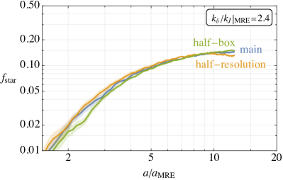
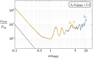
Figure 12: Left: The fraction of dark matter in axion stars for initial conditions with $\left.k_{\delta}/k_{J}\right|_{\rm MRE}=2.4$ in our main simulation runs (‘main’) and simulations with the comoving box size reduced by a factor of $2$ (‘half-box’) and with the comoving lattice spacing increased by a factor of $2$ (‘half-resolution’). Right: The maximum density obtained in simulations with initial $\left.k_{\delta}/k_{J}\right|_{\rm MRE}=2.4$ for simulations using the timestep of our main runs (‘$\Delta_{{t^{\prime}}}$’) and using a timestep that is a factor of $3$ smaller (‘$\Delta_{{t^{\prime}}}$/3’).

The values of $Lk_{\delta}$, $\Delta_{t}$, $N$ and $a_{\rm max}$ required to avoid significant systematic uncertainties depend on the initial $k_{\delta}$ because this determines e.g. when overdensities collapse. We have analyzed the uncertainties for each initial $k_{\delta}$; here we simply report a representative example for $\left.k_{\delta}/k_{J}\right|_{\rm MRE}=2.4$. In Figure 12 left, we plot $f_{\rm star}$ for our main data set (with initial $Lk_{\delta}=24$, timestep $\Delta_{{t^{\prime}}}=0.00015$ and $N^{3}=1152^{3}$) and also with $L$ smaller by a factor of $2$ (with $L/N$ unchanged) and with comoving lattice spacing a factor of $2$ larger. The data obtained with smaller $L$ agrees well with the main data set. The results with the comoving lattice spacing twice as large agree with the main data up to $a/a_{\rm MRE}\simeq 10$ after which there is a deviation. Given that finite lattice spacing effects are expected to enter via the combination $\Delta_{x}/\lambda_{J}(\rho_{s})$ (where $\lambda_{J}(\rho_{s})$ is the quantum Jeans length in the core of an axion star), this suggests that our main data set is safe up to $a/a_{\rm MRE}\simeq 20$. Meanwhile in Figure 12 right we show the maximum density in simulations carried out with our main timestep $\Delta_{{t^{\prime}}}$ and with the timestep a factor of $3$ smaller, with both starting from identical initial conditions. We only have sufficient computational resources to evolve the simulation with $\Delta_{{t^{\prime}}}/3$ to $a/a_{\rm MRE}=6$, but up to this time the differences between the two runs are small and do not accumulate.

We have also checked that starting simulations at $a/a_{\rm MRE}=0.001$ or $0.1$, an order of magnitude smaller or larger than used in our main runs, does not change the results.

C.2 Additional uncertainties

In our simulations around MRE we take the initial axion energy spectrum to be given by eq. (42) with shape parameter $s=4$. To estimate the uncertainty from this assumption, we carry out simulations with initial $\left.k_{p}/k_{J}\right|_{\rm MRE}=0.55$ and with parameters $s=2$ and $6$ (this $k_{p}$ corresponds to initial $\left.k_{\delta}/k_{J}\right|_{\rm MRE}=1.2$ for $s=4$ and slightly different $k_{\delta}$ for the other $s$). In Figure 13 left we plot the corresponding initial $\mathcal{P}_{\delta}$ while in the right panel we show the resulting $f_{\rm star}$. The order-one differences in the initial $\mathcal{P}_{\delta}$ change the asymptotic $f_{\rm star}$ by approximately $25\%$. Meanwhile, the mass of the axion stars that the majority of the bound axions are in, $\bar{M}$, differ by approximately $10\%$ between the different $s$. Thus our main qualitative conclusions are robust against the details of the shape of the initial spectrum for a particular $k_{p}$.

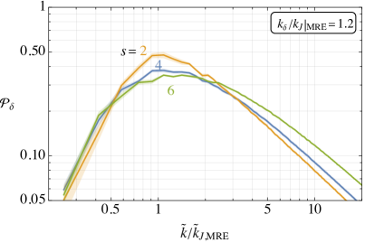
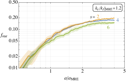
Figure 13: Left: The initial axion density power spectrum $\mathcal{P}_{\delta}$ for initial conditions with different shape parameters $s=2,4,6$ in eq. (42). In each case $\left.k_{p}/k_{J}\right|_{\rm MRE}=0.55$. Right: The fraction of axions in stars $f_{\rm star}$ in simulations starting from the initial conditions in the left panel, with statistical uncertainties.

Another uncertainty comes from our criteria for classifying a collapsed object as an axion star. As discussed in Section 4.1, for our main plots we demand that an object’s spherically averaged density profile matches the soliton form within a factor of $2$ at a distance $r$ of $\lambda_{J}(\rho_{c})/4$ and $\lambda_{J}(\rho_{c})/2$ from the star center. In Figure 14, we compare the inferred $f_{\rm star}$ with that obtained using different criteria (in particular, requiring that at the same $r$ the density profile matches the star form within a factor $1.5$ or that the radial derivative of the quantum pressure matches that of the gravitational potential to within a factor of $2$). The resulting change in $f_{\rm star}$ is typically $25\%$, and possibly as large as $50\%$ for initial $\left.k_{\delta}/k_{J}\right|_{\rm MRE}=0.3$. Although not negligible, this does not significantly affect our main conclusions. We also expect that objects in which quantum pressure is relevant will evolve towards ground state axion stars at times beyond the range of simulations, e.g. as quasi-normal modes decay.

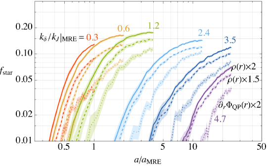
Figure 14: $f_{\rm star}$ obtained with different criteria for identifying stars: “$\rho(r)\times 2$” by demanding that the spherically averaged density profile $\rho(r)$ agrees with the soliton prediction within a factor of $2$ at radius $\lambda_{J}(\rho_{c})/4$ and $\lambda_{J}(\rho_{c})/2$ (as used for our results in the main text); “$\rho(r)\times 1.5$” similar but demanding agreement within a factor of $1.5$ at the same radius; “$\partial_{r}\Phi_{\rm QP}\times 2$” requiring that the radial derivative of the spherically averaged quantum pressure $|\partial_{r}\Phi_{\rm QP}|$ matches the radial derivative of the gravitational potential within a factor of $2$ at the same points.

C.3 Further results from simulations

Here we present additional results from numerical simulations of the axion field around MRE, which support our discussion in Section 4.1.

C.3.1 Collapse of overdensities

In Figure 15 left we plot the maximum energy density in a single simulation run as a function of $a/a_{\rm MRE}$ for each initial $k_{\delta}$ (and also for initial $\left.k_{\delta}/k_{J}\right|_{\rm MRE}=0.15$ smaller than in our other plots, for which resolution of the collapsed objects is lost soon after formation). This is not a well-defined physical observable because the results depend on the simulation volume, but it gives useful intuition. As expected, quantum pressure delays the collapse of overdensities until progressively later times for larger initial $k_{\delta}$, playing a role even for $\left.k_{\delta}/k_{J}\right|_{\rm MRE}=0.3$. At collapse there is a factor of $10$ to $100$ increase in the maximum density, which is subsequently approximately constant and decoupled from the Hubble expansion. This corresponds to the center of the most dense object, with oscillations due to the excited quasi-normal modes of the axion stars.

In Figure 15 right we plot the mean spherically averaged density profile of all objects identified as axion stars for different initial conditions. Prior to averaging, the profile of each object is normalized to its central density $\rho_{s}$ and the associated quantum Jeans length $\lambda_{J}(\rho_{s})$, such that an axion star’s profile takes a universal form independent of its mass. All the averaged profiles match the axion star prediction closely for $r\lesssim 0.75\lambda_{J}(\rho_{s})$, but deviate at larger $r$. For initial $\left.k_{\delta}/k_{J}\right|_{\rm MRE}\gtrsim 2$ the averaged density profiles take a remarkably consistent form with the results for $\left.k_{\delta}/k_{J}\right|_{\rm MRE}=2.4,~{}3.5,~{}4.7$ basically coinciding and having a power law dependence at $r\gtrsim\lambda_{J}(\rho_{s})$. For smaller initial $k_{\delta}$ the averaged density profile switches to a power law form at increasingly small $r/\lambda_{J}(\rho_{s})$. For all initial conditions, the power law is well fit by $\rho(r)\propto r^{-2.5}$, however our results are not sufficient to distinguish between this and e.g. an NFW profile.

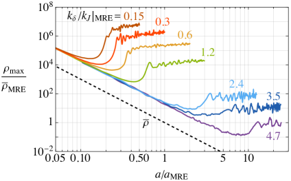
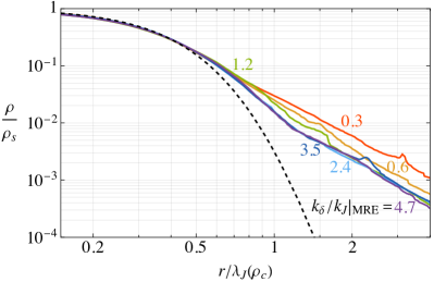
Figure 15: Left: The maximum density in a particular simulation $\rho_{\rm max}$ compared to the mean dark matter density at MRE $\bar{\rho}_{\rm MRE}$. The mean dark matter density $\bar{\rho}(a)$ is also plotted. The collapse of overdensities into gravitationally bound objects decoupled from the Hubble expansion is evident. Right: The average density profile of objects identified as axion stars for different initial conditions, normalized to the objects’ central densities $\rho_{s}$ and the associated quantum Jeans length $\lambda_{J}(\rho_{s})$. Results are shown at the final simulation time for each set of initial conditions. In this way, the axion star profile takes a universal form, plotted in black.

In Figure 16 we plot the comoving axion density power spectrum $\mathcal{P}_{\delta}(\tilde{k})$ at different times for initial conditions with $\left.k_{\delta}/k_{J}\right|_{\rm MRE}=0.3$ and $4.7$.

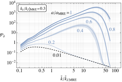
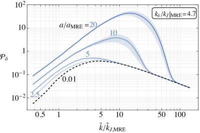
Figure 16: Left: The comoving axion density power spectrum $\mathcal{P}_{\delta}(\tilde{k})$ at different times for initial conditions with $\left.k_{\delta}/k_{J}\right|_{\rm MRE}=0.3$, where $\tilde{k}_{J,{\rm MRE}}$ is the comoving momentum corresponding to the quantum Jeans momentum at MRE. Right: As in the left panel but with initial $\left.k_{\delta}/k_{J}\right|_{\rm MRE}=4.7$, in which case quantum pressure delays gravitational collapse of overdensities until $a/a_{\rm MRE}\simeq 5$.

For initial $\left.k_{\delta}/k_{J}\right|_{\rm MRE}=0.3$, $\mathcal{P}_{\delta}$ starts to increase already at $a/a_{\rm MRE}=0.2$ corresponding to collapse of overdensities evident by $a/a_{\rm MRE}=0.4$ (consistent with the results in Figure 15 left). Meanwhile, for initial $\left.k_{\delta}/k_{J}\right|_{\rm MRE}=4.7$ quantum pressure results in $\mathcal{P}_{\delta}$ remaining frozen until $a/a_{\rm MRE}\simeq 5$ at which time the comoving quantum Jeans length locally to the largest overdensities has decreased enough for them to collapse.

C.3.2 Properties of the axion stars

To further analyze the formation of stars, in Figure 17 left we plot the distribution of $f_{\rm star}$ with axion star mass: $df_{\rm star}/d\log_{10}M_{s}$ at different times for initial conditions with $\left.k_{\delta}/k_{J}\right|_{\rm MRE}=2.4$.

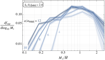
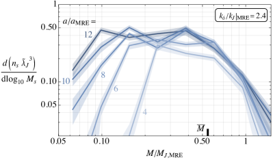
Figure 17: Left: The distribution of the fraction of dark matter bound in axion stars per logarithmic interval of axion star mass, $df_{\rm star}/d\log_{10}M_{s}$, at different times for initial conditions with $\left.k_{\delta}/k_{J}\right|_{\rm MRE}=2.4$. The bands are the statistical uncertainties on the results. Right: The distribution of the axion star number density $n_{s}$ (normalised to $\tilde{\lambda}_{J}^{3}\equiv\lambda_{J,{\rm MRE}}^{3}(a/a_{\rm MRE})^{-3}$, i.e. the comoving volume equal to a quantum Jeans volume at MRE) with axion star mass $M_{s}$. As in the left panel, results are shown at different times with initial conditions with $\left.k_{\delta}/k_{J}\right|_{\rm MRE}=2.4$, with statistical uncertainties.

A burst of relatively heavy stars with masses $\simeq M_{J,{\rm MRE}}/2$ form at $2\lesssim a/a_{\rm MRE}\lesssim 4$ corresponding to the collapse of order-one overdensities (these make up a substantial fraction of the asymptotic $f_{\rm star}$, c.f. Figure 3). Subsequently, $df_{\rm star}/d\log_{10}M_{s}$ is almost time-independent at such masses. However, progressively smaller mass axion stars continue to form due to the collapse of overdensities on smaller scales as $\tilde{k}_{J}(\bar{\rho})$ slowly increases (these do not contribute much to the total $f_{\rm star}$). This can be seen clearly in Figure 17 right, in which we plot the distribution of axion star number density with axion star mass. Although $f_{\rm star}$ is dominated by high masses, smaller and smaller mass stars continue to form and reach number densities comparable to those of the heavy stars.

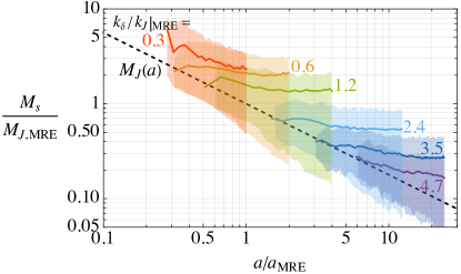
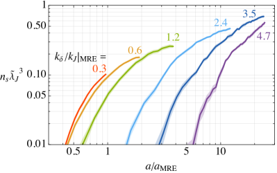
Figure 18: Left: The evolution of $\bar{M}_{s}$, defined by eq. (15), which measures the typical mass of the axion stars that contain the majority of bound axions. The colored bands show the interval containing $90\%$ of axion stars by number (with $5\%$ of stars are more massive and $5\%$ less massive. Right: The number density of identified axion stars per comoving volume $n_{s}$ normalised to $\tilde{\lambda}_{J}^{3}\equiv\lambda_{J,{\rm MRE}}^{3}(a/a_{\rm MRE})^{-3}$, with statistical uncertainties.

Meanwhile, in Figure 18 left, we plot $\bar{M}$, defined in eq. (15), as a function of time for different initial conditions. The colored bands in this plot indicate the distribution of axion star masses with $5\%$ of stars having mass greater than the upper edge of the bands and $5\%$ having mass smaller than the lower edge. For initial $\left.k_{\delta}/k_{J}\right|_{\rm MRE}\in[0.6,3.5]$, $\bar{M}$ reaches an approximately constant value by the final simulation time, which is consistent with $f_{\rm star}$ saturating. Nevertheless, the lower edges of the bands still decrease as successively lighter axion stars continue to form. For initial $\left.k_{\delta}/k_{J}\right|_{\rm MRE}=0.3$ resolution of the axion star cores is lost before $\bar{M}$ and $f_{\rm star}$ presumably reach constant values, while for $\left.k_{\delta}/k_{J}\right|_{\rm MRE}=4.7$ we do not have sufficient computational resources to evolve until $\bar{M}$ reaches a constant value at $a/a_{\rm MRE}\gtrsim 20$. For initial $\left.k_{\delta}/k_{J}\right|_{\rm MRE}\gtrsim 1$, $\bar{M}_{s}$ roughly matches the prediction in eq. (14) with $\delta\simeq 10$. Meanwhile, for initial $\left.k_{\delta}/k_{J}\right|_{\rm MRE}\lesssim 1$, $\bar{M}_{s}$ is smaller than this estimate, which is consistent with a smaller fraction of the axions in the original overdensity being in the central axion star in this case.

Finally, in Figure 18 right we plot the number of axion stars per comoving $\lambda_{J,{\rm MRE}}^{3}(a/a_{\rm MRE})^{-3}$ volume as a function of time. This continues to grow throughout the simulations for all initial conditions. The rate of increase of the number of axion stars slows towards the final simulation times for initial $0.6\lesssim\left.k_{\delta}/k_{J}\right|_{\rm MRE}\lesssim 3.5$. Consistent with our analysis in Section 3, this suggests that the majority of the initially order-one overdensities on length scales of order $k_{p}^{-1}$ have collapsed by the end of the simulations for such initial conditions (with only a few additional, lower mass, stars continuing to form). For initial $\left.k_{\delta}/k_{J}\right|_{\rm MRE}=4.7$ the number of axion stars is still increasing fast at the final simulation time, which is consistent with our expectation that the fraction of axions bound in stars $f_{\rm star}$ will continue to increase beyond the range of simulations in this case. Additionally, for $\left.k_{\delta}/k_{J}\right|_{\rm MRE}=0.3$ the increase in the number of stars shows no sign of slowing before the end of the simulations.

References

- [1] R.. Peccei and Helen R. Quinn “CP Conservation in the Presence of Instantons” In Phys. Rev. Lett. 38, 1977, pp. 1440–1443 DOI: 10.1103/PhysRevLett.38.1440
- [2] Steven Weinberg “A New Light Boson?” In Phys. Rev. Lett. 40, 1978, pp. 223–226 DOI: 10.1103/PhysRevLett.40.223
- [3] Frank Wilczek “Problem of Strong and Invariance in the Presence of Instantons” In Phys. Rev. Lett. 40, 1978, pp. 279–282 DOI: 10.1103/PhysRevLett.40.279
- [4] John Preskill, Mark B. Wise and Frank Wilczek “Cosmology of the Invisible Axion” In Phys. Lett. B 120, 1983, pp. 127–132 DOI: 10.1016/0370-2693(83)90637-8
- [5] L.. Abbott and P. Sikivie “A Cosmological Bound on the Invisible Axion” In Phys. Lett. B 120, 1983, pp. 133–136 DOI: 10.1016/0370-2693(83)90638-X
- [6] Michael Dine and Willy Fischler “The Not So Harmless Axion” In Phys. Lett. B 120, 1983, pp. 137–141 DOI: 10.1016/0370-2693(83)90639-1
- [7] P. Sikivie “Of Axions, Domain Walls and the Early Universe” In Phys. Rev. Lett. 48, 1982, pp. 1156–1159 DOI: 10.1103/PhysRevLett.48.1156
- [8] A. Vilenkin and A.E. Everett “Cosmic Strings and Domain Walls in Models with Goldstone and PseudoGoldstone Bosons” In Phys. Rev. Lett. 48, 1982, pp. 1867–1870 DOI: 10.1103/PhysRevLett.48.1867
- [9] Richard Lynn Davis “Cosmic Axions from Cosmic Strings” In Phys. Lett. B 180, 1986, pp. 225–230 DOI: 10.1016/0370-2693(86)90300-X
- [10] Diego Harari and P. Sikivie “On the Evolution of Global Strings in the Early Universe” In Phys. Lett. B 195, 1987, pp. 361–365 DOI: 10.1016/0370-2693(87)90032-3
- [11] Andrei D. Linde and David H. Lyth “Axionic domain wall production during inflation” In Phys. Lett. B 246, 1990, pp. 353–358 DOI: 10.1016/0370-2693(90)90613-B
- [12] David H. Lyth and Ewan D. Stewart “Axions and inflation: String formation during inflation” In Phys. Rev. D 46, 1992, pp. 532–538 DOI: 10.1103/PhysRevD.46.532
- [13] Peter W. Graham et al. “Experimental Searches for the Axion and Axion-Like Particles” In Ann. Rev. Nucl. Part. Sci. 65, 2015, pp. 485–514 DOI: 10.1146/annurev-nucl-102014-022120
- [14] C.. Hogan and M.. Rees “Axion Miniclusters” In Phys. Lett. B 205, 1988, pp. 228–230 DOI: 10.1016/0370-2693(88)91655-3
- [15] Edward W. Kolb and Igor I. Tkachev “Axion miniclusters and Bose stars” In Phys. Rev. Lett. 71, 1993, pp. 3051–3054 DOI: 10.1103/PhysRevLett.71.3051
- [16] Edward W. Kolb and Igor I. Tkachev “Large amplitude isothermal fluctuations and high density dark matter clumps” In Phys. Rev. D 50, 1994, pp. 769–773 DOI: 10.1103/PhysRevD.50.769
- [17] Kathryn M. Zurek, Craig J. Hogan and Thomas R. Quinn “Astrophysical Effects of Scalar Dark Matter Miniclusters” In Phys. Rev. D 75, 2007, pp. 043511 DOI: 10.1103/PhysRevD.75.043511
- [18] Malcolm Fairbairn, David J.. Marsh and Jérémie Quevillon “Searching for the QCD Axion with Gravitational Microlensing” In Phys. Rev. Lett. 119.2, 2017, pp. 021101 DOI: 10.1103/PhysRevLett.119.021101
- [19] Malcolm Fairbairn, David J.. Marsh, Jérémie Quevillon and Simon Rozier “Structure formation and microlensing with axion miniclusters” In Phys. Rev. D 97.8, 2018, pp. 083502 DOI: 10.1103/PhysRevD.97.083502
- [20] Benedikt Eggemeier et al. “First Simulations of Axion Minicluster Halos” In Phys. Rev. Lett. 125.4, 2020, pp. 041301 DOI: 10.1103/PhysRevLett.125.041301
- [21] Huangyu Xiao, Ian Williams and Matthew McQuinn “Simulations of axion minihalos” In Phys. Rev. D 104.2, 2021, pp. 023515 DOI: 10.1103/PhysRevD.104.023515
- [22] David Ellis et al. “Structure of axion miniclusters” In Phys. Rev. D 106.10, 2022, pp. 103514 DOI: 10.1103/PhysRevD.106.103514
- [23] Benedikt Eggemeier et al. “Axion minivoids and implications for direct detection” In Phys. Rev. D 107.8, 2023, pp. 083510 DOI: 10.1103/PhysRevD.107.083510
- [24] Giovanni Pierobon et al. “Miniclusters from axion string simulations”, 2023 arXiv:2307.09941 [hep-ph]
- [25] Benedikt Eggemeier, Ananthu Krishnan Anilkumar and Klaus Dolag “Evidence for axion miniclusters with an increased central density”, 2024 arXiv:2402.18221 [astro-ph.CO]
- [26] Philippe Jetzer “Boson stars” In Phys. Rept. 220, 1992, pp. 163–227 DOI: 10.1016/0370-1573(92)90123-H
- [27] Jens C. Niemeyer “Small-scale structure of fuzzy and axion-like dark matter”, 2019 DOI: 10.1016/j.ppnp.2020.103787
- [28] I.. Tkachev “On the possibility of Bose star formation” In Phys. Lett. B 261, 1991, pp. 289–293 DOI: 10.1016/0370-2693(91)90330-S
- [29] Edward Seidel and Wai-Mo Suen “Formation of solitonic stars through gravitational cooling” In Phys. Rev. Lett. 72, 1994, pp. 2516–2519 DOI: 10.1103/PhysRevLett.72.2516
- [30] D.. Semikoz and I.. Tkachev “Condensation of bosons in kinetic regime” In Phys. Rev. D 55, 1997, pp. 489–502 DOI: 10.1103/PhysRevD.55.489
- [31] Benedikt Eggemeier and Jens C. Niemeyer “Formation and mass growth of axion stars in axion miniclusters” In Phys. Rev. D 100.6, 2019, pp. 063528 DOI: 10.1103/PhysRevD.100.063528
- [32] Marco Gorghetto, Edward Hardy and Giovanni Villadoro “Axions from Strings: the Attractive Solution” In JHEP 07, 2018, pp. 151 DOI: 10.1007/JHEP07(2018)151
- [33] Marco Gorghetto, Edward Hardy and Giovanni Villadoro “More axions from strings” In SciPost Phys. 10.2, 2021, pp. 050 DOI: 10.21468/SciPostPhys.10.2.050
- [34] Malte Buschmann et al. “Dark matter from axion strings with adaptive mesh refinement” In Nature Commun. 13.1, 2022, pp. 1049 DOI: 10.1038/s41467-022-28669-y
- [35] Ken’ichi Saikawa, Javier Redondo, Alejandro Vaquero and Mathieu Kaltschmidt “Spectrum of global string networks and the axion dark matter mass”, 2024 arXiv:2401.17253 [hep-ph]
- [36] Heejoo Kim, Junghyeon Park and Minho Son “Axion Dark Matters from Cosmic String Network”, 2024 arXiv:2402.00741 [hep-ph]
- [37] C. Hagmann and P. Sikivie “Computer simulations of the motion and decay of global strings” In Nucl. Phys. B 363, 1991, pp. 247–280 DOI: 10.1016/0550-3213(91)90243-Q
- [38] R.A. Battye and E.P.S. Shellard “Global string radiation” In Nucl. Phys. B 423, 1994, pp. 260–304 DOI: 10.1016/0550-3213(94)90573-8
- [39] Masahide Yamaguchi, M. Kawasaki and Jun’ichi Yokoyama “Evolution of axionic strings and spectrum of axions radiated from them” In Phys. Rev. Lett. 82, 1999, pp. 4578–4581 DOI: 10.1103/PhysRevLett.82.4578
- [40] C. Hagmann, Sanghyeon Chang and P. Sikivie “Axion radiation from strings” In Phys. Rev. D 63, 2001, pp. 125018 DOI: 10.1103/PhysRevD.63.125018
- [41] Takashi Hiramatsu et al. “Improved estimation of radiated axions from cosmological axionic strings” In Phys. Rev. D 83, 2011, pp. 123531 DOI: 10.1103/PhysRevD.83.123531
- [42] Takashi Hiramatsu, Masahiro Kawasaki, Ken’ichi Saikawa and Toyokazu Sekiguchi “Production of dark matter axions from collapse of string-wall systems” [Erratum: Phys.Rev.D 86, 089902 (2012)] In Phys. Rev. D 85, 2012, pp. 105020 DOI: 10.1103/PhysRevD.85.105020
- [43] Masahiro Kawasaki, Ken’ichi Saikawa and Toyokazu Sekiguchi “Axion dark matter from topological defects” In Phys. Rev. D 91.6, 2015, pp. 065014 DOI: 10.1103/PhysRevD.91.065014
- [44] Leesa Fleury and Guy D. Moore “Axion dark matter: strings and their cores” In JCAP 01, 2016, pp. 004 DOI: 10.1088/1475-7516/2016/01/004
- [45] Vincent B. Klaer and Guy D. Moore “How to simulate global cosmic strings with large string tension” In JCAP 10, 2017, pp. 043 DOI: 10.1088/1475-7516/2017/10/043
- [46] Vincent B.. Klaer and Guy D. Moore “The dark-matter axion mass” In JCAP 11, 2017, pp. 049 DOI: 10.1088/1475-7516/2017/11/049
- [47] Masahiro Kawasaki, Toyokazu Sekiguchi, Masahide Yamaguchi and Jun’ichi Yokoyama “Long-term dynamics of cosmological axion strings” In PTEP 2018.9, 2018, pp. 091E01 DOI: 10.1093/ptep/pty098
- [48] Vincent B. Klaer and Guy D. Moore “Global cosmic string networks as a function of tension” In JCAP 06, 2020, pp. 021 DOI: 10.1088/1475-7516/2020/06/021
- [49] M.. Khlopov, B.. Malomed, Ia.. Zeldovich and Ya.. Zeldovich “Gravitational instability of scalar fields and formation of primordial black holes” In Mon. Not. Roy. Astron. Soc. 215.4, 1985, pp. 575–589 DOI: 10.1093/mnras/215.4.575
- [50] Wayne Hu, Rennan Barkana and Andrei Gruzinov “Cold and fuzzy dark matter” In Phys. Rev. Lett. 85, 2000, pp. 1158–1161 DOI: 10.1103/PhysRevLett.85.1158
- [51] Marco Gorghetto et al. “Dark photon stars: formation and role as dark matter substructure” In JCAP 08.08, 2022, pp. 018 DOI: 10.1088/1475-7516/2022/08/018
- [52] Marco Gorghetto and Edward Hardy “Post-inflationary axions: a minimal target for axion haloscopes” In JHEP 05, 2023, pp. 030 DOI: 10.1007/JHEP05(2023)030
- [53] David J. Gross, Robert D. Pisarski and Laurence G. Yaffe “QCD and Instantons at Finite Temperature” In Rev. Mod. Phys. 53, 1981, pp. 43 DOI: 10.1103/RevModPhys.53.43
- [54] Sz. Borsanyi et al. “Calculation of the axion mass based on high-temperature lattice quantum chromodynamics” In Nature 539.7627, 2016, pp. 69–71 DOI: 10.1038/nature20115
- [55] Edward W. Kolb and Igor I. Tkachev “Nonlinear axion dynamics and formation of cosmological pseudosolitons” In Phys. Rev. D 49, 1994, pp. 5040–5051 DOI: 10.1103/PhysRevD.49.5040
- [56] Alejandro Vaquero, Javier Redondo and Julia Stadler “Early seeds of axion miniclusters” In JCAP 04, 2019, pp. 012 DOI: 10.1088/1475-7516/2019/04/012
- [57] D.. Levkov, A.. Panin and I.. Tkachev “Gravitational Bose-Einstein condensation in the kinetic regime” In Phys. Rev. Lett. 121.15, 2018, pp. 151301 DOI: 10.1103/PhysRevLett.121.151301
- [58] P. Sikivie and Q. Yang “Bose-Einstein Condensation of Dark Matter Axions” In Phys. Rev. Lett. 103, 2009, pp. 111301 DOI: 10.1103/PhysRevLett.103.111301
- [59] Jonas Enander, Andreas Pargner and Thomas Schwetz “Axion minicluster power spectrum and mass function” In JCAP 12, 2017, pp. 038 DOI: 10.1088/1475-7516/2017/12/038
- [60] Lam Hui “Wave Dark Matter” In Ann. Rev. Astron. Astrophys. 59, 2021, pp. 247–289 DOI: 10.1146/annurev-astro-120920-010024
- [61] P. Meszaros “The behaviour of point masses in an expanding cosmological substratum.” In aap 37.2, 1974, pp. 225–228
- [62] Julio F. Navarro, Carlos S. Frenk and Simon D.. White “The Structure of cold dark matter halos” In Astrophys. J. 462, 1996, pp. 563–575 DOI: 10.1086/177173
- [63] Mateja Gosenca, Julian Adamek, Christian T. Byrnes and Shaun Hotchkiss “3D simulations with boosted primordial power spectra and ultracompact minihalos” In Phys. Rev. D 96.12, 2017, pp. 123519 DOI: 10.1103/PhysRevD.96.123519
- [64] Remo Ruffini and Silvano Bonazzola “Systems of selfgravitating particles in general relativity and the concept of an equation of state” In Phys. Rev. 187, 1969, pp. 1767–1783 DOI: 10.1103/PhysRev.187.1767
- [65] M. Membrado, A.. Pacheco and J. Sañudo “Hartree solutions for the self-Yukawian boson sphere” In Phys. Rev. A 39 American Physical Society, 1989, pp. 4207–4211 DOI: 10.1103/PhysRevA.39.4207
- [66] Pierre-Henri Chavanis and Luca Delfini “Mass-radius relation of Newtonian self-gravitating Bose-Einstein condensates with short-range interactions. II. Numerical results” In Physical Review D 84.4 American Physical Society (APS), 2011 DOI: 10.1103/physrevd.84.043532
- [67] F.. Guzman “Oscillation modes of ultralight BEC dark matter cores” In Phys. Rev. D 99.8, 2019, pp. 083513 DOI: 10.1103/PhysRevD.99.083513
- [68] James Hung-Hsu Chan, Sergey Sibiryakov and Wei Xue “Boson star normal modes” In JHEP 08, 2023, pp. 045 DOI: 10.1007/JHEP08(2023)045
- [69] Xiaolong Du, Bodo Schwabe, Jens C. Niemeyer and David Bürger “Tidal disruption of fuzzy dark matter subhalo cores” In Phys. Rev. D 97.6, 2018, pp. 063507 DOI: 10.1103/PhysRevD.97.063507
- [70] Virgile Dandoy, Thomas Schwetz and Elisa Todarello “A self-consistent wave description of axion miniclusters and their survival in the galaxy” In JCAP 09, 2022, pp. 081 DOI: 10.1088/1475-7516/2022/09/081
- [71] V.. Dokuchaev, Yu.. Eroshenko and I.. Tkachev “Destruction of axion miniclusters in the Galaxy” In J. Exp. Theor. Phys. 125.3, 2017, pp. 434–442 DOI: 10.1134/S1063776117080039
- [72] Bradley J. Kavanagh, Thomas D.. Edwards, Luca Visinelli and Christoph Weniger “Stellar disruption of axion miniclusters in the Milky Way” In Phys. Rev. D 104.6, 2021, pp. 063038 DOI: 10.1103/PhysRevD.104.063038
- [73] Xuejian Shen, Huangyu Xiao, Philip F. Hopkins and Kathryn M. Zurek “Disruption of Dark Matter Minihalos in the Milky Way Environment: Implications for Axion Miniclusters and Early Matter Domination” In Astrophys. J. 962.1, 2024, pp. 9 DOI: 10.3847/1538-4357/ad12c6
- [74] Ian DSouza and Chris Gordon “The Disruption of Dark Matter Minihalos by Successive Stellar Encounters”, 2024 arXiv:2402.03236 [astro-ph.GA]
- [75] Xiaolong Du et al. “Soliton merger rates and enhanced axion dark matter decay” In Phys. Rev. D 109.4, 2024, pp. 043019 DOI: 10.1103/PhysRevD.109.043019
- [76] Dennis Maseizik and Günter Sigl “Distributions and Collision Rates of ALP Stars in the Milky Way”, 2024 arXiv:2404.07908 [astro-ph.CO]
- [77] Bodo Schwabe, Jens C. Niemeyer and Jan F. Engels “Simulations of solitonic core mergers in ultralight axion dark matter cosmologies” In Phys. Rev. D 94.4, 2016, pp. 043513 DOI: 10.1103/PhysRevD.94.043513
- [78] K. Kuijken and G. Gilmore “The Mass Distribution in the Galactic Disc - Part Two - Determination of the Surface Mass Density of the Galactic Disc Near the Sun” In Mon. Not. Roy. Astron. Soc. 239, 1989, pp. 605
- [79] Chris Flynn et al. “On the mass-to-light ratio of the local Galactic disc and the optical luminosity of the Galaxy” In Mon. Not. Roy. Astron. Soc. 372, 2006, pp. 1149–1160 DOI: 10.1111/j.1365-2966.2006.10911.x
- [80] Andrew J. Benson “Orbital parameters of infalling dark matter substructures” [Erratum: Mon.Not.Roy.Astron.Soc. 364, 1104 (2005)] In Mon. Not. Roy. Astron. Soc. 358, 2005, pp. 551–562 DOI: 10.1111/j.1365-2966.2005.08788.x
- [81] P. Brun “A new experimental approach to probe QCD axion dark matter in the mass range above 40 eV” In Eur. Phys. J. C 79.3, 2019, pp. 186 DOI: 10.1140/epjc/s10052-019-6683-x
- [82] Jesse Liu “Broadband solenoidal haloscope for terahertz axion detection”, 2021 arXiv:2111.12103 [physics.ins-det]
- [83] Peter Tinyakov, Igor Tkachev and Konstantin Zioutas “Tidal streams from axion miniclusters and direct axion searches” In JCAP 01, 2016, pp. 035 DOI: 10.1088/1475-7516/2016/01/035
- [84] Ciaran A.. O’Hare, Giovanni Pierobon and Javier Redondo “Axion minicluster streams in the solar neighbourhood”, 2023 arXiv:2311.17367 [hep-ph]
- [85] Hsi-Yu Schive, Tzihong Chiueh and Tom Broadhurst “Cosmic Structure as the Quantum Interference of a Coherent Dark Wave” In Nature Phys. 10, 2014, pp. 496–499 DOI: 10.1038/nphys2996
- [86] Bodo Schwabe et al. “Simulating mixed fuzzy and cold dark matter” In Phys. Rev. D 102.8, 2020, pp. 083518 DOI: 10.1103/PhysRevD.102.083518
- [87] Hsi-Yu Schive et al. “Understanding the Core-Halo Relation of Quantum Wave Dark Matter from 3D Simulations” In Phys. Rev. Lett. 113.26, 2014, pp. 261302 DOI: 10.1103/PhysRevLett.113.261302
- [88] Edward W. Kolb and Igor I. Tkachev “Femtolensing and picolensing by axion miniclusters” In Astrophys. J. Lett. 460, 1996, pp. L25–L28 DOI: 10.1086/309962
- [89] Andrey Katz, Joachim Kopp, Sergey Sibiryakov and Wei Xue “Femtolensing by Dark Matter Revisited” In JCAP 12, 2018, pp. 005 DOI: 10.1088/1475-7516/2018/12/005
- [90] Liang Dai and Jordi Miralda-Escudé “Gravitational Lensing Signatures of Axion Dark Matter Minihalos in Highly Magnified Stars” In Astron. J. 159.2, 2020, pp. 49 DOI: 10.3847/1538-3881/ab5e83
- [91] Michal Cuadrat-Grzybowski et al. “Probing Primordial Black Holes and Dark Matter Clumps in the Solar System with Gravimeter and GNSS Networks”, 2024 arXiv:2403.14397 [astro-ph.CO]
- [92] Joerg Jaeckel, Sebastian Schenk and Michael Spannowsky “Probing dark matter clumps, strings and domain walls with gravitational wave detectors” In Eur. Phys. J. C 81.9, 2021, pp. 828 DOI: 10.1140/epjc/s10052-021-09604-9
- [93] Hyungjin Kim “Gravitational interaction of ultralight dark matter with interferometers” In JCAP 12, 2023, pp. 018 DOI: 10.1088/1475-7516/2023/12/018
- [94] I.. Tkachev “Fast Radio Bursts and Axion Miniclusters” In JETP Lett. 101.1, 2015, pp. 1–6 DOI: 10.1134/S0021364015010154
- [95] Aiichi Iwazaki “Fast Radio Bursts from Axion Stars”, 2014 arXiv:1412.7825 [hep-ph]
- [96] Stuart Raby “Axion star collisions with Neutron stars and Fast Radio Bursts” In Phys. Rev. D 94.10, 2016, pp. 103004 DOI: 10.1103/PhysRevD.94.103004
- [97] Yang Bai and Yuta Hamada “Detecting Axion Stars with Radio Telescopes” In Phys. Lett. B 781, 2018, pp. 187–194 DOI: 10.1016/j.physletb.2018.03.070
- [98] James H. Buckley, P.. Dev, Francesc Ferrer and Fa Peng Huang “Fast radio bursts from axion stars moving through pulsar magnetospheres” In Phys. Rev. D 103.4, 2021, pp. 043015 DOI: 10.1103/PhysRevD.103.043015
- [99] Samuel J. Witte et al. “Transient radio lines from axion miniclusters and axion stars” In Phys. Rev. D 107.6, 2023, pp. 063013 DOI: 10.1103/PhysRevD.107.063013
- [100] Chris Kouvaris, Tao Liu and Kun-Feng Lyu “Radio signals from axion star-neutron star binaries” In Phys. Rev. D 109.2, 2024, pp. 023008 DOI: 10.1103/PhysRevD.109.023008
- [101] Aiichi Iwazaki “Radiation burst by axion star collision with star in the Andromeda Galaxy” In Phys. Lett. B 829, 2022, pp. 137089 DOI: 10.1016/j.physletb.2022.137089
- [102] A. Kyriazis “Dilute axion stars converting to photons in the Milky Way’s magnetic field” In JHEP 12, 2023, pp. 164 DOI: 10.1007/JHEP12(2023)164
- [103] Thomas W. Kephart and Thomas J. Weiler “Stimulated radiation from axion cluster evolution” In Phys. Rev. D 52, 1995, pp. 3226–3238 DOI: 10.1103/PhysRevD.52.3226
- [104] Eric Braaten, Abhishek Mohapatra and Hong Zhang “Emission of Photons and Relativistic Axions from Axion Stars” In Phys. Rev. D 96.3, 2017, pp. 031901 DOI: 10.1103/PhysRevD.96.031901
- [105] D.. Levkov, A.. Panin and I.. Tkachev “Radio-emission of axion stars” In Phys. Rev. D 102.2, 2020, pp. 023501 DOI: 10.1103/PhysRevD.102.023501
- [106] Giovanni Grilli di Cortona, Edward Hardy, Javier Pardo Vega and Giovanni Villadoro “The QCD axion, precisely” In JHEP 01, 2016, pp. 034 DOI: 10.1007/JHEP01(2016)034
- [107] Jiajun Chen, Xiaolong Du, Erik Lentz and David J.. Marsh “Relaxation times for Bose-Einstein condensation by self-interaction and gravity” In Phys. Rev. D 106.2, 2021, pp. 023009 DOI: 10.1103/PhysRevD.106.023009
- [108] Kay Kirkpatrick, Anthony E. Mirasola and Chanda Prescod-Weinstein “Analysis of Bose-Einstein condensation times for self-interacting scalar dark matter” In Phys. Rev. D 106.4, 2022, pp. 043512 DOI: 10.1103/PhysRevD.106.043512
- [109] Mudit Jain, Wisha Wanichwecharungruang and Jonathan Thomas “Kinetic relaxation and nucleation of Bose stars in self-interacting wave dark matter” In Phys. Rev. D 109.1, 2024, pp. 016002 DOI: 10.1103/PhysRevD.109.016002
- [110] Mudit Jain, Mustafa A. Amin, Jonathan Thomas and Wisha Wanichwecharungruang “Kinetic relaxation and Bose-star formation in multicomponent dark matter” In Phys. Rev. D 108.4, 2023, pp. 043535 DOI: 10.1103/PhysRevD.108.043535
- [111] Raphael Micha and Igor I. Tkachev “Turbulent thermalization” In Phys. Rev. D 70, 2004, pp. 043538 DOI: 10.1103/PhysRevD.70.043538
- [112] Marco Gorghetto, Edward Hardy and Horia Nicolaescu “Observing invisible axions with gravitational waves” In JCAP 06, 2021, pp. 034 DOI: 10.1088/1475-7516/2021/06/034
- [113] Faber Edwards, Emily Kendall, Shaun Hotchkiss and Richard Easther “PyUltraLight: A Pseudo-Spectral Solver for Ultralight Dark Matter Dynamics” In JCAP 10, 2018, pp. 027 DOI: 10.1088/1475-7516/2018/10/027