An LSTM Feature Imitation Network for Hand Movement Recognition from sEMG Signals

Abstract

Surface Electromyography (sEMG) is a non-invasive signal that is used in the recognition of hand movement patterns, the diagnosis of diseases, and the robust control of prostheses. Despite the remarkable success of recent end-to-end Deep Learning approaches, they are still limited by the need for large amounts of labeled data. To alleviate the requirement for big data, researchers utilize Feature Engineering, which involves decomposing the sEMG signal into several spatial, temporal, and frequency features. In this paper, we propose utilizing a feature-imitating network (FIN) for closed-form temporal feature learning over a 300ms signal window on Ninapro DB2, and applying it to the task of 17 hand movement recognition. We implement a lightweight LSTM-FIN network to imitate four standard temporal features (entropy, root mean square, variance, simple square integral). We then explore transfer learning capabilities by applying the pre-trained LSTM-FIN for tuning to a downstream hand movement recognition task. We observed that the LSTM network can achieve up to 99% R2 accuracy in feature reconstruction and 80% accuracy in hand movement recognition. Our results also showed that the model can be robustly applied for both within- and cross-subject movement recognition, as well as simulated low-latency environments. Overall, our work demonstrates the potential of the FIN modeling paradigm in data-scarce scenarios for sEMG signal processing.

I Introduction

The Surface Electromyography (sEMG) signal is a highly valuable indicator of electro-physiological activity in both the medical and engineering fields [1]. As a non-invasive method, it can be easily measured using electrodes and is widely used in human-computer interfaces as a control input, such as in the control of prostheses [2]. However, interpreting sEMG signals to determine a subject’s movement intention can be challenging. Surface EMG signals are non-linear, variable [3], and can be easily contaminated by electromagnetic noise, baseline drift, and noise from electronic components [4]. Additionally, inaccuracies in electrode placement can also affect the accuracy of sEMG measurements [5], and introduce sensitivies to environmental changes [6].

A typical procedure for utilizing sEMG in machine learning consists of: (1) data pre-processing [7], which includes denoising and normalization while preserving as much of the original information as possible, (2) feature extraction, which involves identifying useful time [8], frequency [9], time-frequency [10], and spatial features [8] from the sEMG signal; (3) classification/regression, in which the extracted features are mapped to a label (such as hand gesture recognition).

Feature engineering has led foundational improvements in recognition quality through extracting mathematically defined (and meaningful) representations from the original signal [11]; in general, better quality features often results in better performing models. Traditional time-domain features that are frequently used include Zero-Crossing (ZC), Mean Absolute Variance (MAV), and Root Mean Square (RMS) [12]. Frequency domain features include Median Frequency (MDF) [13] and Fast Fourier Transform (FFT) [14]. Common techniques for feature extraction in the Time-frequency Domain (TFD) include the Wavelet Transform (WT) and short-time Fourier Transform (STFT) [15].

However, the learning quality of feature engineering is directly dependent on the feature selection process [16]. Unlike feature engineering, the feature representations in deep learning methods are automatically (implicitly) learned in the network’s hidden layers. These techniques train the model end-to-end, specifically, learning the mapping from original data to classification labels directly, bypassing the feature-selection and feature-classification mapping procedures of conventional methods [17]. Deep learning networks have the natural advantage of automatically learning feature representations using a variety of network architectures (convolutional, recurrent, feedforward, capsule [18], and transformer neural network architectures [19]). The learned feature representations are abstract and typically beyond a closed-form mathematical description (i.e. uninterpretable) [20, 21, 22]. In this work, we aim to demonstrate the viability of pre-training networks with an explicit set of manually selected time-domain features, taking advantage of knowledge distilled from feature engineering efforts while also balancing the flexibility provided by deep learning methods to tune and adapt learned representations.

Contemporary research efforts have focused on end-to-end training approaches [23], yet a common concern of end-to-end training approaches is that it is highly data-intensive [12]. The end-to-end model is expected to adapt to various environmental scenarios such as electrode shifts [24], muscle fatigue [25], and variations between subjects [25]. However, each scenario requires re-sampling and re-training. Obtaining such large datasets can be a significant challenge due to the logistics required to recruit human subjects and configure the experiment, which makes data collection difficult to scale.

A common solution to data scarcity is to replace the end-to-end training paradigm with feature-to-end transfer learning [13]. The model’s parameters are trained on feature representations directly on one domain and then transferred and tuned for classification and reconstruction tasks, reducing the need for large amounts of training data and time [26]. While the feature-to-end transfer learning approach has been actively explored, the end-to-feature modeling paradigm has been less explored, but is increasingly finding appeal in the context of self-supervised learning [27]. A novel approach in this domain are Feature Imitation Networks (FIN), which have shown state-of-the-art performance on several biomedical signal and image processing tasks [28]. However, there has been no prior work to evaluate the potential of FINs for sEMG signal processing tasks. In this paper, our aim is to explore the end-to-feature learning approach by utilizing a set of established time-domain sEMG features (we emphasize that this is distinct from the conventional end-to-end or feature-to-end learning approaches). Specifically, our aim is to apply a temporal network architecture, in the form of a FIN, to imitate time-domain features [28]. The pre-trained FINs are then fine-tuned for downstream classification tasks (by feeding into a feature-to-end model).

I-A Contributions

Our work has four contributions to the domain of deep learning and sEMG signal processing: (1) we propose an LSTM-based FIN for closed-form temporal feature learning and demonstrate its ability to learn closed-form feature representations, including Entropy (ENT), Root Mean Square (RMS), Variance (VAR), and Simple Square Integral (SSI). (2) We demonstrate the applicability of our LSTM-FIN on a downstream hand movement classification task, outperforming the baseline CNN classifier using ground-truth features. (3) We evaluate the transfer learning capabilities of the LSTM-FIN to unseen subjects. (4) We explore generating future feature values from current time windows to evaluate overall model classification performance in a simulated low-latency scenario.

Novelty: The novelty of this work presents itself in an LSTM FIN that learns closed-form temporal feature representations, that can be flexibly tuned for downstream classification tasks; we demonstrate that the LSTM FIN enhances classification task performance, robustly transfers to unseen subjects, and generates features more applicable to low-latency scenarios compared to conventional neural learning approaches.

II Data and Methods

II-A Data Acquisition

In order to compare our work with published benchmarks, we utilized the widely-used NinaPro dataset as our primary data source [29]. Specifically, we selected Exercise B of the DB2 database, which includes 8 isometric and isotonic hand configurations and 9 basic movements of the wrist (excluding rests), for a total of 17 movements. The dataset includes sEMG data collected from 12 electrodes placed on the right forearm of 40 intact subjects; 12 female and 28 male subjects. Each movement was repeated 6 times, with a 5-second hold, and a 3-second rest period between repetitions. The data was collected at a 2 kHz sampling rate, with a total sampling duration of over 500 seconds for each subject.

II-B Target Variable

We were interested in classifying hand movements from 17 hand movements recorded in the data; therefore, the target variable was a one-hot vector, representing the hand movements (i.e. 1 of 17 classes).

II-C Data Splits

To maintain consistency with the data split method of the dataset [29], where repetitions 2 and 5 were designated as the test set, while repetitions 1, 3, 4, and 6 were allocated for the training set. We followed this method as a fundamental framework and further subdivided the training set into pre-training and fine-tuning subsets. In order to explore the model’s transfer learning ability across subjects, we subsequently divided a “within-subjects”(1-25) and a “cross-subjects” (26-40). Specifically, repetitions 1, 3, and 4 of subjects 1-25 were used for pre-training, and repetition 6 was employed for fine-tuning. For subjects 26-40, repetitions 1, 3, 4, and 6 were utilized for fine-tuning. Repetitions 2 and 5 of all subjects were collectively employed as the test set. The intuitive representation of the data split is shown in the figure 1.

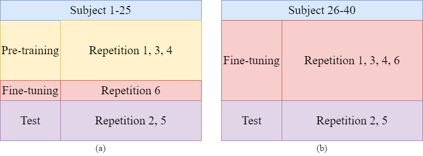
Figure 1: Data split using NinaPro DB2. The yellow section is the pre-training set, the pink section is the fine-tuning set, and the purple section is the test set. Rows are the repetitions while columns are the subject IDs.

II-D Data Normalization

To ensure that the sEMG signals recorded across the different channels were within a similar scale, zero-mean and unit-variance (i.e. Z-score) normalization was applied to each channel [30].

II-E Input structure

The model data inputs were generated using a sliding window of 300ms with a stride of 10ms. A 300ms window size is commonly used in the literature [31, 30], as it strikes a balance between providing enough continuous data for a network to learn patterns while minimizing perceptible delays when a model is deployed for real-time human interaction scenarios [32]. Given the sampling rate of 2KHz, a 300ms window resulted in 600 sample points per window and 20 sample points per stride. A final window size of 600x12 was utilized, where 12 represents the 12 electrode channels.

II-F Features

A wide range of time-domain features have been successfully applied to sEMG signals for gesture prediction. Many of these features capture correlating information, thus utilizing just a subset of features quickly saturates model performance [12]. Furthermore, studies have shown that time domain features are often redundant for the task [17]. Therefore, our work focuses on four widely explored features that capture complementary information, and which have also been shown to be independently predictive: Entropy (ENT), Root Mean Square (RMS), Variance (VAR), and Simple Square Integral (SSI) [12].

The motivation for choosing these 4 features is to suggest to the network what features have the most significant impact on classification accuracy. In which RMS is a representation of constant force and non-fatiguing contraction in the signal [33]; VAR measures the degree to which the signal varies within a small window, with higher values indicating greater signal vibration[34]; Entropy represents the irregularity of a specific signal, with higher values indicating higher irregularity[35]; SSI represents the accumulated energy in a single window, with higher values indicating more energy concentrated in that channel [36]. It should be noted that these four features are on different scales, therefore, we apply zero-mean unit-variance normalization (i.e. z-score) to each feature set.

III Model Architecture

In this study, the architecture is divided into two parts: the upstream part is a bi-directional LSTM FIN that approximates time-domain features. The downstream part is a classifier that maps the features to hand movement.

Figure 2: Bi-directional Feature Imitating LSTM Neural Network; 3-layer structure, each layer has 600 forward-backward connected LSTM cells. Each LSTM-FIN learns to generate one of four features (RMS, VAR, ENT, SSI).

III-A Baseline Feature Imitating LSTM

LSTMs have been widely used for extracting temporal features in time series regression tasks [37, 30, 38]. Bidirectional LSTMs (Bi-LSTM) further improve upon LSTMs by learning both forward and backward relationships [39], and has been shown to handle data where inputs and targets are not perfectly aligned point-wise [40]. Hence, we utilize Bi-LSTMs as the FIN architecture since the closed-form representations the model would learn are time-domain features (not frequency-domain features for which CNNs excel at learning [41]).

The baseline LSTM-FIN model is designed as a 3-layer bidirectional LSTM model, with 600x2 LSTM cells in each layer and 32 hidden units in each cell. Parameters are optimized with grid search. Since the goal is to imitate the features of a given channel, the input dimension is set to 1. The output of the LSTM is taken from the hidden size of the last cell of the last layer and then fed into a fully connected perceptron that generates one feature output. The LSTM-FIN structure is illustrated in figure 2. The total number of trainable parameters in the LSTM is 22,508.

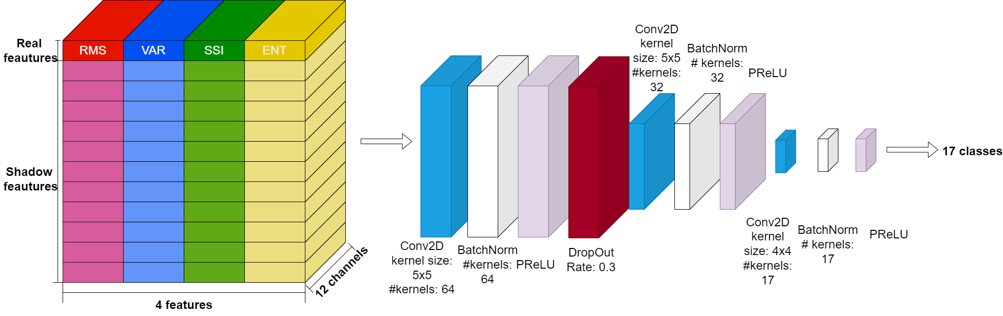
Figure 3: Downstream neural network architecture for hand movement recognition. The input is composed of ground-truth features and their shadow variations (via gaussian perturbation) for CNN-pre-training.

III-B Feature Augmentation

The function of the downstream classifier is to map the imitated features to the subject’s hand movement (i.e. gesture). However, due to the scarce nature of the imitated feature matrix ($4\times 12$ feature matrix), to improve the classifier’s accuracy and robustness, a feature augmentation method is introduced before the classifier.

In the context of feature augmentation, due to the significant differences in absolute values among the four features, we treat them as four distinct channels. For each sampling window, we generate 12 one-dimensional corresponding features for each feature channel based on the sampling electrodes. Typically, for one-dimensional features, we employ the practice of adding random noise to augment the features [42]. Therefore, for each feature, we replicate it an additional 11 times and introduce Gaussian noise with a mean of 0 and a standard deviation of 0.01. These augmented features are then stacked along the dimension of the original feature, resulting in the creation of a two-dimensional $12\times 12$ feature matrix for each feature. By doing so, we expand the feature matrices into a $4\times 12\times 12$ tensor, making them suitable for subsequent use with neural networks designed for image processing and classification.

III-C Downstream Classifier

The augmented feature tensor is then trained using a three-layer network, where each layer contains a 2D convolutional layer, a batch normalizing layer, and a PReLU activation layer. A dropout layer with a rate of 0.3 is added between the first and second modules to discard outlier features randomly. Finally, we produce an output layer consisting of 17 neurons, corresponding to movements 1 through 17 (figure 3).

IV Experiments

In this section, we discuss configurations of experiments for (1) training and evaluating the LSTM-FIN network, (2) applying the trained LSTM-FIN to hand movement classification tasks, (3) configuring tasks to predict “forward-in-time”, and (4) baseline models.

IV-A Exp. $\#$1: Feature Imitating Experiment

For training the LSTM-FIN, an early stopping procedure was applied once the training converged to prevent overfitting; the Adam optimizer was used during training with an initial learning rate of 0.001 and weight decay of $2\times 10^{-5}$.

For evaluation, we compared the model’s output with the closed-form (ground truth) feature values and assessed accuracy using two metrics: R-squared (R²) and Mean Absolute Percentage (MAP). The former metric shows how well the data fit the regression model; the closer from 1, the better the regression is. While the latter metric offers an intuitive difference comparison between imitated feature and ground truth by proportion.

IV-B Exp. $\#$2: Forward-in-time Prediction

To experimentally assess the LSTM-FIN’s ability to predict future feature values, we varied the prediction window stride, considering future prediction horizons of: 50ms, 100ms, 150ms, 200ms, 250ms, and 300ms.

IV-C Exp. $\#$3: Downstream CNN Training

In order to examine the CNN’s ability to classify based on the FIN-extracted features and evaluate its performance in a subject-specific manner, two scenarios were designed to test the CNN’s classification ability based on the extracted features.

Scenario 1 involved training the CNN using the training set and the fine-tuning set, which consisted of repetitions 1, 3, 4, and 6 from subjects 1 to 25. The testing set, on the other hand, comprised repetitions 2 and 5 of subjects 1 to 40. During testing, subject-by-subject evaluation was conducted to quantify model performance for each individual subject. We term this as “multi-subject” training.

Scenario 2 involved tuning the CNN using the fine-tuning set from scratch. The initial training was performed across the whole training set (and excluded the fine-tuning set), while tuning and testing were performed subject-by-subject to quantify model performance for each individual subject. We term this as “single-subject” training.

IV-D Exp. #4: Downstream Fine-tuning Experiments

For this experiment, our aim was to combine these two models (LSTM-FIN and CNN). We first pre-trained the LSTM-FIN and downstream CNN classifier separately with the original data and the calculated ground-truth features on the training set. Subsequently, we performed fine-tuning on this combined model with the fine-tuning set.

As for the fine-tuning part, we initialized the encoder (LSTM-FIN) and decoder (CNN) models with their respective pre-trained weights obtained from the training on the corresponding subjects. We then integrated the encoder and decoder models and enabled weight back-propagation on both parts of the network. Next, we reloaded the fine-tuning set (repetition 6 of subjects 1 to 25 and repetitions 1, 3, 4, and 6 of subjects 26 to 40), and fine-tuned the model as a whole. During the fine-tuning, the model would learn to adapt to a specific subject, so as to increase the accuracy of the classification tasks.

TABLE I: LSTM-FIN Model Performance Results

Feature	$R^{2}$	MAP
ENT	0.98 (±0.10)	95.17% (±11.78%)
RMS	0.99 (±0.08)	95.33% (±9.47%)
SSI	0.96 (±0.14)	88.62% (±14.43%)
VAR	0.98 (±0.12)	92.97% (±1306%)

Figure 4: Boxplot of $R^{2}$ accuracy distribution of LSTM-FIN model.

V Results and Discussion

V-A Feature Imitating Network Performance

The feature imitating capability of the LSTM-FIN is characterized by the MAP and $R^{2}$ accuracy, which were evaluated on the test set. The distribution of the $R^{2}$ accuracy is illustrated in Figure 4(a).

From the statistical results, we observe that the FIN exhibits strong feature imitation capabilities for the four temporal features ($R^{2}$ $>$ 0.96 and MAP $>$ 88%). Furthermore, from the distribution plots, we can observe that the accuracy distribution for all 4 features are centered close to 1, indicating that FIN can imitate the features extremely well. However, beyond the plots, we observe most outliers are centered near 0, suggesting that in some cases, the FIN may incorrectly imitate the features, and when it does so, it is almost completely incorrect. There is a minimal occurrence of intermediate values between perfect imitation and complete mismatch. The result in turn shows the overall robustness of LSTM-FINs in learning feature representations.

V-B Downstream Classification Performance

Next, we will discuss the performance of three classification models. We examined four scenarios: (1) SVM model with a Gaussian kernel using the ground-truth features, CNN models trained on ground-truth features using either, (2) multi-subject training (denoted CNN-I), or (3) single-subject training (denoted CNN-II), (4) LSTM + CNN-II model trained using the raw sEMG data, and (5) LSTM-FIN + CNN-II model, which involved feature imitation using FINs trained on the raw sEMG data and fine-tuning it on the fine-tuning set. For the final two models, CNN-II was utilized as a pre-trained model.

We evaluate the accuracy of these models in within-subject recognition and cross-subject recognition based on 100% usage of the fine-tuning set data. The results of these evaluations are presented in table II.

The results in table II provide insights into the performance of each model in different scenarios. The accuracy values indicate the model’s ability to correctly classify the 17 hand movements within the same subject group (within-subject recognition) and across different subject groups (cross-subject recognition).

TABLE II: Machine Learning Model Performance Results

Feature Inputs	Model	Accuracy
		(mean ± std)
Within-Subject (1-25)
ENT, RMS, SSI, VAR	CNN-I	29.40% ± 2.00%
ENT, RMS, SSI, VAR	CNN-II	64.64% ± 7.70%
ENT, RMS, SSI, VAR	SVM	53.59% ± 6.47%
Raw sEMG	LSTM + CNN-II	34.57% ± 8.35%
Raw sEMG	LSTM-FIN + CNN-II	65.70% ± 7.50%
Cross-Subject (26-40)
ENT, RMS, SSI, VAR	CNN-I	25.13% ± 1.94%
ENT, RMS, SSI, VAR	CNN-II	77.90% ± 7.19%
ENT, RMS, SSI, VAR	SVM	52.91% ± 7.70%
Raw sEMG	LSTM + CNN-II	45.41% ± 6.33%
Raw sEMG	LSTM-FIN + CNN-II	80.06% ± 6.21%
All-Subject (1-40)
ENT, RMS, SSI, VAR	CNN-I	27.80% ± 1.98%
ENT, RMS, SSI, VAR	CNN-II	69.61% ± 9.86%
ENT, RMS, SSI, VAR	SVM	52.94% ± 8.42%
Raw sEMG	LSTM + CNN-II	38.64% ± 9.25%
Raw sEMG	LSTM-FIN + CNN-II	71.8% ± 9.89%

Notably, we observe that the CNN-II, LSTM + CNN-II, and LSTM-FIN + CNN-II models performed significantly better in the cross-subject split relative to the within-subject split; 77.90% vs. 64.64%, 45.41% vs. 34.57%, and 80.06% vs. 65.70%, respectively. This may be because more repetitions were included in the cross-subject experiments, which provided more variety of data, improving the model’s generalizability of recognizing inter-repetition samples. The result, in turn, demonstrates the viability of implementing transfer learning for cross-subject recognition.

When comparing the performance of models that derived their representations from the raw sEMG signal we observe that the LSTM model outperforms (by 2+%) the other models when pre-trained as a FIN, however, when trained to automatically learn representations from scratch, the LSTM + CNN-II significantly under-performs (by 14+%) models trained with the ground-truth features directly as input (CNN-II, SVM). In both cases, the LSTM + CNN-II models had the same architecture, so the difference in performance may be because imitating features (defined due to years of feature engineering efforts [11], and of predictive value as evidenced by the SVM performance) significantly decreases the search space, making it easier for the model to learn these representations directly than trying to learn them for scratch while optimizing for the downstream classification task.

V-B1 Model Training Time

We also compared the training performance of the model in pre-training and fine-tuning, as shown in table III. CNN-I and CNN-II are not included in the fine-tuning process since they are directly trained. FIN represents its pre-training process, while FIN+CNN represents the fine-tuning process when the LSTM-FIN and CNN-II are combined. From the data in the table, we observe that the FIN has a relatively large number of parameters, so it needs a longer time for pre-training. However, it converges within the smallest number of epochs (3 epochs). CNN-II only uses data from a single subject, so its training speed is significantly faster; 0.46s per epoch. CNN-II also converges within a relatively smaller number of epochs (12 epochs) compared to CNN-I (31 epochs). As for the fine-tuning process of the FIN-CNN, it converges within a relatively short number of epochs (4 epochs) and in less than four minutes. This relatively short-time for tuning makes the FIN-CNN applicable to practical problems that require rapid adaptation for single-subject use.

TABLE III: Average number of epochs to converge and average epoch time

Model	# Epoch to Converge	Epoch time
CNN-I	31	12s
CNN-II	12	0.46s
LSTM + CNN-II	5	26s
LSTM-FIN + CNN-II	4	58s
LSTM-FIN	3	98s

V-C Fine-tuning Model Performance

Figure 6 illustrates the average performance of the FIN-CNN network in real-time, i.e., without predicting future features, with different proportions of training data. The percentages represent the actual number of data windows used for fine-tuning as a percentage of the total number of windows in the fine-tuning set. It is important to note that in the fine-tuning process, three additional repetitions, namely repetitions 1,3, and 4, were predominantly used for across-subjects fine-tuning. Therefore, the actual data used in across-subjects was nearly 3 times more than the within-subjects set given the same percentage. However, even though across-subjects contained more repetitions, 100% data usage of the within-subject set is still more than 20% of data usage of the across-subject set. In summary, incorporating more repetitions is far more effective than stacking data from single repetitions; on the other hand, the accuracy is less subjective to the data usage proportion, which guarantees the performance under scarce labeled data circumstances.

V-D Forward-in-time Classification

In our experiments, we also considered the possibility of predicting future actions. Therefore, we trained the models for different prediction time steps and evaluated their ability to predict future actions. For the CNN-II model, the results are presented in figure 5(a) and figure 5(b). Figure 5(a) displays the average prediction accuracy on the across-subjects data that was trained using multiple repetitions, while figure 5(b) illustrates the average prediction accuracy for all 40 subjects.

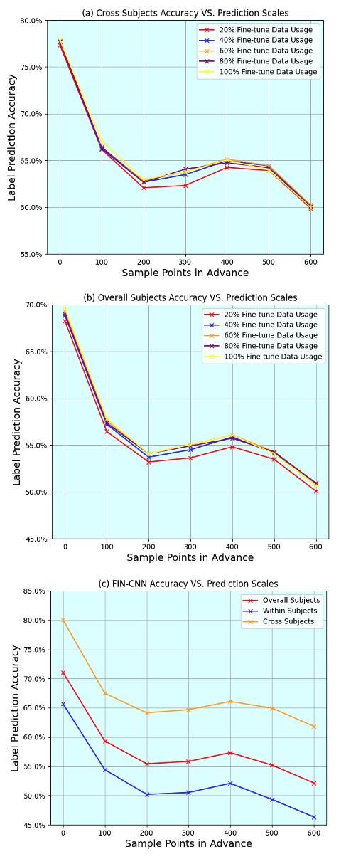
Figure 5: Mean accuracy of FIN-CNN model, x-axis represents the sample points the model is predicting ahead (100 points is 50ms), y-axis represents model classification accuracy. Sub-figure (a) shows the accuracy variation on subjects 26-40; Sub-figure (b) shows the overall accuracy variation on subjects 1-40; Sub-figure (c) enumerates the model’s performance based on different test sets.

In the plots, accuracy curves with different data usage proportions generally overlap each other, indicating again that the CNN model is not sensitive to the proportion of data usage. However, the across-subjects set achieved higher accuracy as the set contains more variations of repetitions. This highlights the importance of utilizing a diverse range of repetitions during training, as it enables the model to learn more comprehensive and representative patterns within the data.

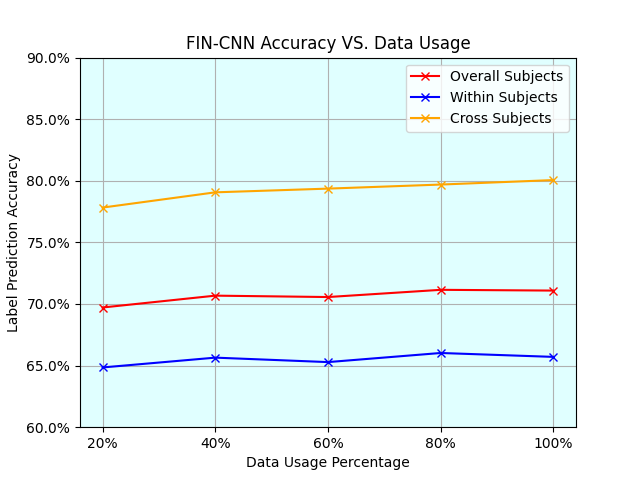
Figure 6: Mean accuracy of LSTM-FIN + CNN-II model, showing percentage of data used (x-axis) during training versus model classification accuracy (y-axis).

We also conducted similar experiments for the FIN-CNN model. The accuracy-proportion curve in figure 6 shows a nearly flat trend. Similar to the CNN model (figure 5(a) and figure 5(b)), increasing the amount of data from existing repetitions has minimal impact on the accuracy. However, when we refer to test sets that incorporated different repetitions (figure 5(c)), the curve shows significant gaps while maintaining the same trend. This further confirms our observation that even with limited data availability, the FIN-CNN model performs well in the classification task. However, to improve the accuracy, it is necessary to incorporate more repetitions into the training process. When predicting hand movements up to 600 points (300ms) into the future, we observe a general degradation in performance (from approximately 70% to 50% accuracy overall); however, for scenarios where near real-time prediction is more important than accuracy, or for which predictions may be retrospectively corrected, such a level of performance may still be meaningful.

VI Conclusion

In this paper, we explore the application of FINs to represent four temporal sEMG signal features. We augmented the temporal features using shadow dilation and used them to learn a mapping to hand movement classification using a CNN model. The experiments demonstrated that the FIN, implemented as an LSTM, could accurately simulate temporal features with a strong accuracy exceeding 96% R2 and 88% MAP. The CNN classifier with feature dilation outperformed traditional SVM classifiers in terms of recognition accuracy. Furthermore, when leveraging the enhanced generalization capability of FIN, we observed that the FIN-CNN hybrid model (with transferred FIN model and fine-tuning) achieved superior classification performance compared to using a CNN alone.

We also investigated scenarios of models trained with partial amounts of data. The results confirmed that even with limited labeled data, the model was still able to perform well in the downstream classification task. However, incorporating more repetitions was necessary to improve the model’s accuracy further. We also observed that our models were robust at recognizing both within- and cross-subject hand movements. Additionally, we examined the model’s ability to predict movements in the short-term future (up to 300ms), and while the prediction accuracy was lower than real-time accuracy, the model still exhibited partial capability in this regard. Our work demonstrates the performance of a pre-trained FIN model and its application to a downstream task (via transfer learning) while also addressing issues related to data scarcity and simulated low-latency environments.

For future work, we propose exploring (1) the use of other neural network structures (e.g. CNN, feedforward) as FINs, (2) learning to imitate other time-frequency features, with the aim of creating robust and interpretable neural network models. We propose (3) investigating the proposed approach for transfer learning between intact and amputated populations, a challenging transfer learning task, as well as (4) evaluating the forward-in-time classification model with end-users to assess the responsiveness of our approach to real-world use-cases.

References

- [1] R. Merletti and C. J. De Luca, “New techniques in surface electromyography,” Computer Aided EMG and Expert Sys., vol. 9, no. 3, pp. 115–124, 1989.
- [2] X. Navarro, T. B. Krueger, N. Lago, S. Micera, T. Stieglitz, and P. Dario, “A critical review of interfaces with the peripheral nervous system for the control of neuroprostheses and hybrid bionic systems,” J. Peripheral Nervous Sys., vol. 10, no. 3, pp. 229–258, 2005.
- [3] K. A. Farry, I. D. Walker, and R. G. Baraniuk, “Myoelectric teleoperation of a complex robotic hand,” IEEE Trans. on Robotics and Automation, vol. 12, no. 5, pp. 775–788, 1996.
- [4] C. Li, D. Cao, and Y. Yuan, “Research on improved wavelet denoising method for semg signal,” in 2019 Chinese Automation Congress, pp. 5221–5225, IEEE, 2019.
- [5] A. Moin, A. Zhou, A. Rahimi, S. Benatti, A. Menon, S. Tamakloe, J. Ting, N. Yamamoto, Y. Khan, F. Burghardt, et al., “An emg gesture recognition system with flexible high-density sensors and brain-inspired high-dimensional classifier,” in IEEE ISCAS, pp. 1–5, IEEE, 2018.
- [6] M. Simao, N. Mendes, O. Gibaru, and P. Neto, “A review on electromyography decoding and pattern recognition for human-machine interaction,” IEEE Access, vol. 7, pp. 39564–39582, 2019.
- [7] U. BAŞPINAR, V. Y. ŞENYÜREK, B. DOĞAN, and H. S. VAROL, “A comparative study of denoising semg signals,” Turkish Journal of Electrical Eng. and Computer Sciences, vol. 23, no. 4, pp. 931–944, 2015.
- [8] Y. Zhang, Y. Chen, H. Yu, X. Yang, and W. Lu, “Learning effective spatial–temporal features for semg armband-based gesture recognition,” IEEE Internet of Things J., vol. 7, no. 8, pp. 6979–6992, 2020.
- [9] U. C. Allard, F. Nougarou, C. L. Fall, P. Giguère, C. Gosselin, F. Laviolette, and B. Gosselin, “A convolutional neural network for robotic arm guidance using semg based frequency-features,” in IEEE/RSJ IROS, pp. 2464–2470, IEEE, 2016.
- [10] S. Karheily, A. Moukadem, J.-B. Courbot, and D. O. Abdeslam, “semg time–frequency features for hand movements classification,” Expert Sys. with App., vol. 210, p. 118282, 2022.
- [11] A. Phinyomark and E. Scheme, “Emg pattern recognition in the era of big data and deep learning,” Big Data and Cognitive Comp/, vol. 2, no. 3, p. 21, 2018.
- [12] A. Waris and E. N. Kamavuako, “Effect of threshold values on the combination of emg time domain features: Surface versus intramuscular emg,” Biomedical Signal Processing and Control, vol. 45, pp. 267–273, 2018.
- [13] F. Zhuang, Z. Qi, K. Duan, D. Xi, Y. Zhu, H. Zhu, H. Xiong, and Q. He, “A comprehensive survey on transfer learning,” Proceedings of the IEEE, vol. 109, no. 1, pp. 43–76, 2020.
- [14] P. Geethanjali, “Myoelectric control of prosthetic hands: state-of-the-art review,” Medical Devices: Evidence and Research, pp. 247–255, 2016.
- [15] A. Waris, M. Zia ur Rehman, I. K. Niazi, M. Jochumsen, K. Englehart, W. Jensen, H. Haavik, and E. N. Kamavuako, “A multiday evaluation of real-time intramuscular emg usability with ann,” Sensors, vol. 20, no. 12, p. 3385, 2020.
- [16] W. Wei, X. Hu, H. Liu, M. Zhou, Y. Song, et al., “Towards integration of domain knowledge-guided feature engineering and deep feature learning in surface electromyography-based hand movement recognition,” Comp. Intelligence and Neuroscience, vol. 2021, 2021.
- [17] A. Phinyomark, P. Phukpattaranont, and C. Limsakul, “Feature reduction and selection for emg signal classification,” Expert systems with applications, vol. 39, no. 8, pp. 7420–7431, 2012.
- [18] W. Wang, W. You, Z. Wang, Y. Zhao, S. Wei, et al., “Feature fusion-based improved capsule network for semg signal recognition,” Comp. Intell. and Neuro., vol. 2022, 2022.
- [19] M. Montazerin, E. Rahimian, F. Naderkhani, S. F. Atashzar, S. Yanushkevich, and A. Mohammadi, “Transformer-based hand gesture recognition from instantaneous to fused neural decomposition of high-density emg signals,” Scientific reports, vol. 13, no. 1, p. 11000, 2023.
- [20] S.-H. Park and S.-P. Lee, “Emg pattern recognition based on artificial intelligence techniques,” IEEE Trans. on Rehabilitation Engineering, vol. 6, no. 4, pp. 400–405, 1998.
- [21] V. Srhoj-Egekher, M. Cifrek, and S. Peharec, “Feature modeling for interpretable low back pain classification based on surface emg,” IEEE Access, vol. 10, pp. 73702–73727, 2022.
- [22] X. Li, H. Xiong, X. Li, X. Wu, X. Zhang, J. Liu, J. Bian, and D. Dou, “Interpretable deep learning: Interpretation, interpretability, trustworthiness, and beyond,” Knowledge and Information Systems, vol. 64, no. 12, pp. 3197–3234, 2022.
- [23] J. Liu, X. Zhou, B. He, P. Li, C. Wang, and X. Wu, “A novel method for detecting misclassifications of the locomotion mode in lower-limb exoskeleton robot control,” IEEE RA-L, vol. 7, no. 3, pp. 7779–7785, 2022.
- [24] L. Hargrove, K. Englehart, and B. Hudgins, “The effect of electrode displacements on pattern recognition based myoelectric control,” in 2006 IEEE EMBC, pp. 2203–2206, IEEE, 2006.
- [25] A. Phinyomark, F. Quaine, S. Charbonnier, C. Serviere, F. Tarpin-Bernard, and Y. Laurillau, “Emg feature evaluation for improving myoelectric pattern recognition robustness,” Expert Sys. with App., vol. 40, no. 12, pp. 4832–4840, 2013.
- [26] J. Maggu, E. Chouzenoux, G. Chierchia, and A. Majumdar, “Convolutional transform learning,” in ICONIP, Siem Reap, Cambodia, December 13–16, 2018, Proceedings, Part III 25, pp. 162–174, Springer, 2018.
- [27] A. Mohamed, H.-y. Lee, L. Borgholt, J. D. Havtorn, J. Edin, C. Igel, K. Kirchhoff, S.-W. Li, K. Livescu, L. Maaløe, et al., “Self-supervised speech representation learning: A review,” IEEE Journal of Selected Topics in Signal Processing, vol. 16, no. 6, pp. 1179–1210, 2022.
- [28] S. Saba-Sadiya, T. Alhanai, and M. M. Ghassemi, “Feature imitating networks,” in ICASSP 2022-2022 IEEE ICASSP, pp. 4128–4132, IEEE, 2022.
- [29] M. Atzori, A. Gijsberts, C. Castellini, B. Caputo, A.-G. M. Hager, S. Elsig, G. Giatsidis, F. Bassetto, and H. Müller, “Electromyography data for non-invasive naturally-controlled robotic hand prostheses,” Scientific data, vol. 1, no. 1, pp. 1–13, 2014.
- [30] T. Sun, Q. Hu, P. Gulati, and S. F. Atashzar, “Temporal dilation of deep lstm for agile decoding of semg: Application in prediction of upper-limb motor intention in neurorobotics,” IEEE RA-L, vol. 6, no. 4, pp. 6212–6219, 2021.
- [31] H. F. Hassan, S. J. Abou-Loukh, and I. K. Ibraheem, “Teleoperated robotic arm movement using electromyography signal with wearable myo armband,” Journal of King Saud University-Engineering Sciences, vol. 32, no. 6, pp. 378–387, 2020.
- [32] K. Englehart and B. Hudgins, “A robust, real-time control scheme for multifunction myoelectric control,” IEEE Trans. on Biomedical Eng., vol. 50, no. 7, pp. 848–854, 2003.
- [33] J. L. Gennisson, C. Cornu, S. Catheline, M. Fink, and P. Portero, “Human muscle hardness assessment during incremental isometric contraction using transient elastography,” J. of Biomechanics, vol. 38, no. 7, pp. 1543–1550, 2005.
- [34] S. Negi, Y. Kumar, and V. Mishra, “Feature extraction and classification for emg signals using linear discriminant analysis,” in ICACCA, pp. 1–6, IEEE, 2016.
- [35] Y. Cao, W.-w. Tung, J. Gao, V. A. Protopopescu, and L. M. Hively, “Detecting dynamical changes in time series using the permutation entropy,” Physical Review E, vol. 70, no. 4, p. 046217, 2004.
- [36] S. Du and M. Vuskovic, “Temporal vs. spectral approach to feature extraction from prehensile emg signals,” in IRI 2004, pp. 344–350, IEEE, 2004.
- [37] P. Sedighi, X. Li, and M. Tavakoli, “Emg-based intention detection using deep learning for shared control in upper-limb assistive exoskeletons,” IEEE RA-L, vol. 9, no. 1, pp. 41–48, 2024.
- [38] T. Sun, Q. Hu, J. Libby, and S. F. Atashzar, “Deep heterogeneous dilation of lstm for transient-phase gesture prediction through high-density electromyography: Towards application in neurorobotics,” IEEE RA-L, vol. 7, no. 2, pp. 2851–2858, 2022.
- [39] K. Subhash, J. K. Paul, and P. Pournami, “Bi-directional lstm for monitoring biceps brachii muscle activity of healthy subjects using semg signals,” in Intelligent Sys. Conf., pp. 487–499, Springer, 2023.
- [40] C. Ma, C. Lin, O. W. Samuel, W. Guo, H. Zhang, S. Greenwald, L. Xu, and G. Li, “A bi-directional lstm network for estimating continuous upper limb movement from surface electromyography,” IEEE RA-L, vol. 6, no. 4, pp. 7217–7224, 2021.
- [41] Z. Wang, W. Yan, and T. Oates, “Time series classification from scratch with deep neural networks: A strong baseline,” in IJCNN, pp. 1578–1585, IEEE, 2017.
- [42] F. Wang, S.-h. Zhong, J. Peng, J. Jiang, and Y. Liu, “Data augmentation for eeg-based emotion recognition with deep convolutional neural networks,” in MMM Part II 24, pp. 82–93, Springer, 2018.