ACE: A general-purpose non-Markovian open quantum systems simulation toolkit based on process tensors

Abstract

We describe a general-purpose computational toolkit for simulating open quantum systems, which provides numerically exact solutions for composites of zero-dimensional quantum systems that may be strongly coupled to multiple, quite general non-Markovian environments. It is based on process tensor matrix product operators (PT-MPOs), which efficiently encapsulate environment influences. The code features implementations of several PT-MPO algorithms, in particular, Automated Compression of Environments (ACE) for general environments comprised of independent modes as well as schemes for generalized spin boson models. The latter includes a divide-and-conquer scheme for periodic PT-MPOs, which enable million time step simulations for realistic models. PT-MPOs can be precalculated and reused for efficiently probing different time-dependent system Hamiltonians. They can also be stacked together and combined to provide numerically complete solutions of small networks of open quantum systems. The code is written in C++ and is fully controllable by configuration files, for which we have developed a versatile and compact human-readable format.

I Introduction

Many problems in quantum chemistry [1, 2], quantum optics [3, 4], condensed matter physics [5], and quantum information theory [6] take the form of (zero-dimensional) few-level open quantum systems coupled to some environment. If the coupling is weak, standard perturbative and Born-Markov treatments can be employed to derive time-local Lindblad master equations [7, 8], which are straightforward to solve numerically using standard differential equation algorithms [9] or using convenient toolkits such as QuTiP [10] or QuantumOptics.jl [11].

The situation is more challenging when the system-environment coupling is strong and non-Markovian memory effects have to be accounted for [12]. Then, an accurate treatment of environment effects requires modeling—explicitly or implicitly—the quantum dynamical evolution of the environment. Because real environments typically consist of a (quasi)continuum of degrees of freedom or modes, a many-body quantum systems arises, whose direct solution is in general intractable. Most methods for non-Markovian open quantum systems tackle this challenge by focusing on a particular class of problems and make use of the particularities to reduce the problem complexity.

For example, if the environment is one-dimensional [13] or can be mapped onto one dimension [2, 14], tensor network structures like matrix product states (MPSs) and operators (MPOs) [15] provide very efficient numerically tractable representations of the state of the environment. Larger-dimensional environments are often accurately modeled using mean-field or cumulant expansion techniques [16, 17] or treatments motivated by perturbation theory [18].

One of the most widely studied classes of open quantum systems is the spin-boson model, which describes (bio-)molecules [1, 2], resonant nanojunctions [19], as well as semiconductor nanostructures like quantum dots (QDs) [20]. The particular Gaussian character of the linear coupling to a bath of harmonic oscillators enables a treatment using path integrals [21], which has been the basis of, on the one hand, hierarchical equations of motion (HEOM) [22, 23] and, on the other hand, the iterative path integral scheme QUAPI [24, 25]. Both techniques have been further developed [26] and implemented in computer codes like HierarchicalEOM.jl [27] and PathSum [28], respectively.

Only recently a new strategy to describe open quantum systems has emerged: the process tensor (PT) formalism [6, 29]. Here, environment influences are encapsulated and represented in efficient tensor network structures called process tensor matrix product operators (PT-MPOs) [30]. PT-MPOs can be constructed to depend only on the environment Hamiltonian and the system-environment interaction, and describe the impact of the environment irrespective of interventions performed on the system, such as unitary time evolution due to a time-dependent system Hamiltonian or measurements [6] [see Fig. 1(a)]. This has many advantages: First, the numerically challenging part, the PT-MPO calculation, has to be performed only once and the resulting PT-MPO can be reused many times, e.g., to optimize parameters or driving protocols for open quantum systems [31]. Second, the allowed interventions on the system include those needed to extract multi-time correlation functions. This is particularly useful for non-Markovian open quantum systems when the quantum regression theorem no longer holds [32]. Finally, a quantum system coupled to two or more environments can be simulated using two PT-MPOs calculated independently of each other. The result remains numerically exact [33, 30]. This fact can be used to investigate non-additive multi-environment effects [34, 35] [see Fig. 1(b)] as well as cooperative effects in multi-site quantum systems where each site is coupled to a local non-Markovian environment [36]. Due to the modularity and separation of concerns, PT-MPOs are promising for scalable schemes to simulate small to medium-sized quantum networks [37].

The first algorithms to calculate PT-MPOs [29] started from a tensor network derived from path integrals [38], and were thus restricted to Gaussian environments like generalized spin-boson models. These are now implemented in the Python package OQuPy [39]. Subsequently, progress was made in two directions: First, new schemes provide orders-of-magnitude speed-up by employing a divide-and-conquer strategy [40] and periodic PT-MPOs [40, 41]. Second, algorithms for different [42] and more general [33] types of environments have become available. Specifically, in Ref. [33], we introduced the algorithm Automated Compression of Environments (ACE), which is applicable to any environment that can be described in terms of $N_{E}$ independent modes, such as phonon, photon, fermion, spin, and anharmonic environments. Moreover, the environment modes themselves may be subject to Markovian losses and they may be time-dependently driven. Changing the contraction order of the tensor network and employing an efficient ‘preselection’ scheme for the combination of PT-MPOs with large inner bonds yields a variant of ACE which is about one to two orders of magnitude faster [43].

In this article, we describe our accompanying eponymous numerical toolkit ACE [44], which implements the ACE method as well as other PT-MPO techniques. It is designed to allow users to profit from the efficiency, modularity, and generality of PT-MPO techniques without requiring any programming. The physical problem is instead defined in human-readable configuration files, where one specifies the microscopic Hamiltonians, initial states, as well as a set of control and convergence parameters. For convenience, shortcut notations are available for some special and recurring problem classes. One can also easily switch between several algorithms and thus quickly compare their performance and accuracy.

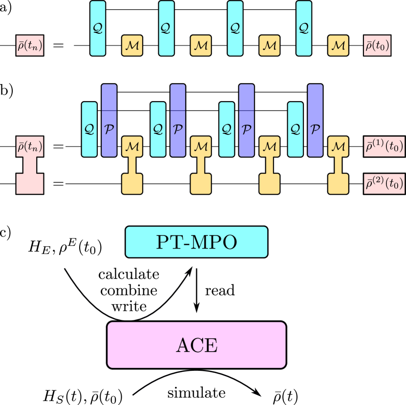
Figure 1: (a): Propagation of a quantum system (reduced density matrix $\bar{\rho}$) coupled to an environment described by a PT-MPO (set of $\mathcal{Q}$’s) and subject to a free system propagator $\mathcal{M}$, which depends on the system Hamiltonian. (b): Example for composition of open quantum systems. Depicted is a bipartite quantum system of interest, whose parts are coupled via the free system propagator $\mathcal{M}$. The upper part of the system is coupled to two (in general non-Markovian) environments, each described by a PT-MPO. (c): Workflow of the ACE code. First, the ACE code can be used calculate a PT-MPO from the microscopic environment Hamiltonian and the initial state of the environment. Optionally the PT-MPO can be written to a file, read from file, and combined with other PT-MPOs. Then, for a given system Hamiltonian and initial state, the reduced density matrix and thereby all system observables can be extracted.

The article is structured as follows: In Sec. II, we summarize the fundamentals of PT-MPOs as well as the implemented methods. In Sec. III, we describe the general usage of the ACE code, which is followed by a series of concrete examples in Sec. IV. A summary of available commands for configuration files is provided in the appendix A.

II Implemented methods 

II.1 PT-MPOs: General principles

The ACE code uses PT-MPOs to numerically exactly simulate non-Markovian open quantum systems. We therefore first sketch the key concepts of PT-MPOs. A more detailed derivation can be found in Ref. [30].

The time evolution of a system (S) together with its environment (E) is formally given by

$$\rho(t)= \overleftarrow{T}\exp\bigg{(}{\int\limits_{0}^{t}d\tau\,\mathcal{L}(\tau)}\bigg{)}\rho(0),$$ (1)

where $\overleftarrow{T}$ is the time ordering operator and $\mathcal{L}$ is the total Liouvillian, which determines the time evolution $\dot{\rho}(t)=\mathcal{L}(t)\rho(t)$, e.g., $\mathcal{L}\rho=-\frac{i}{\hbar}[H,\rho]$ with total Hamiltonian $H$. The total Liouvillian

$$\mathcal{L}= \mathcal{L}_{S}+\mathcal{L}_{E}$$ (2)

is split into a part $\mathcal{L}_{S}$, which only affects system degrees of freedom, and an environment part $\mathcal{L}_{E}$, which affects both, the environment and the system, as it also includes the system-environment interaction. Next, one introduces a time grid $t_{j}=t_{0}+j\Delta t$ with steps $\Delta t$, which is chosen small enough to ensure (i) that $\mathcal{L}$ can be considered constant in time over the time step $\Delta t$ and (ii) that the error of the Trotter splitting

$$e^{\mathcal{L}\Delta t}=e^{\mathcal{L}_{E}\Delta t}e^{\mathcal{L}_{S}\Delta t}+\mathcal{O}(\Delta t^{2})$$ (3)

is small enough. Tracing over the environment at the final time step $t_{n}=t$ yields the reduced system density matrix $\bar{\rho}(t)=\textrm{Tr}_{E}\big{\{}\rho(t)\big{\}}$

$$\bar{\rho}(t)= \textrm{Tr}_{E}\Big{\{}e^{\mathcal{L}_{E}\Delta t}e^{\mathcal{L}_{S}\Delta t}\dots e^{\mathcal{L}_{E}\Delta t}e^{\mathcal{L}_{S}\Delta t}\bar{\rho}(0)\otimes\rho^{E}(0)\Big{\}},$$ (4)

where we additionally assume that the total system initially factorizes $\rho(0)=\bar{\rho}(0)\otimes\rho^{E}(0)$ in system and environment parts. Collecting all terms relating to the environment, we rewrite Eq. (4) as

$$\bar{\rho}_{\alpha_{n}}= \sum_{\begin{subarray}{c}\alpha_{n-1},\ldots,\alpha_{0}\\ \alpha^{\prime}_{n},\ldots,{\alpha}^{\prime}_{1}\end{subarray}}\mathcal{I}^{(\alpha_{n},{\alpha}^{\prime}_{n})\ldots(\alpha_{1},{\alpha}^{\prime}_{1})}\bigg{(}\prod_{l=1}^{n}\mathcal{M}^{\alpha^{\prime}_{l}\alpha_{l-1}}\bigg{)}\bar{\rho}_{\alpha_{0}},$$ (5)

where we have introduced the notation that left and right system indices $\nu_{j},\mu_{j}$ on the density matrix at time $t_{j}$ are combined to a single Liouville space index $\alpha_{j}=(\nu_{j},\mu_{j})$ and the time argument is implied in the sub-index, e.g, $\bar{\rho}_{\alpha_{j}}=\bar{\rho}_{\nu_{j},\mu_{j}}(t_{j})$. Furthermore, $\mathcal{M}^{\alpha^{\prime}_{l}\alpha_{l-1}}=\big{(}e^{\mathcal{L}_{S}\Delta t}\big{)}_{(\nu^{\prime}_{l},\mu^{\prime}_{l}),(\nu_{l-1},\mu_{l-1})}$ is the explicit matrix representation of the system propagator $e^{\mathcal{L}_{S}\Delta t}$ and $\mathcal{I}^{(\alpha_{n},{\alpha}^{\prime}_{n})\ldots(\alpha_{1},{\alpha}^{\prime}_{1})}$ is the generalized Feynman-Vernon influence functional [21].

Eq. (5) is universally valid and exact up to the (controllable) Trotter error, but it suffers from exponential scaling of the number of summands with the number of time steps. PT-MPOs address this by representing the generalized influence functional in matrix product operator form

$$\mathcal{I}^{(\alpha_{n},\alpha^{\prime}_{n})\ldots(\alpha_{1},\alpha^{\prime}_{1})}$$

$$\quad\quad\;=\sum_{d_{n},\dots,d_{0}}\mathcal{Q}^{(\alpha_{n},\alpha^{\prime}_{n})}_{d_{n}d_{n-1}}\mathcal{Q}^{(\alpha_{n-1},\alpha^{\prime}_{n-1})}_{d_{n-1}d_{n-2}}\ldots\mathcal{Q}^{(\alpha_{1},\alpha^{\prime}_{1})}_{d_{1}d_{0}},$$ (6)

which can be viewed as a series of matrix products with respect to inner bonds $d_{l}$. On the edges, the inner bonds only take one value $d_{n}=d_{0}=0$.

Then, Eq. (5) becomes

$$\bar{\rho}_{\alpha_{n}}= \sum_{d_{n}}q_{d_{n}}\bigg{(}\prod_{l=1}^{n}\sum_{\alpha^{\prime}_{l},\alpha_{l-1},d_{l-1}}\!\!\!\mathcal{Q}^{(\alpha_{l},{\alpha}^{\prime}_{l})}_{d_{l},d_{l-1}}\mathcal{M}^{\alpha^{\prime}_{l}\alpha_{l-1}}\bigg{)}\bar{\rho}_{\alpha_{0}}\delta_{d_{0},0},$$ (7)

which can be propagated time step by time step, and thus reduces the numerical complexity from exponential to polynomial in the number of time steps. The reduced system density matrix at intermediate time steps can be obtained my contracting the inner bond $d_{n}$ with the closure $q_{d_{n}}$, which can be calculated from the PT-MPO as discussed in Ref. [33]. Equation (7) is visualized in Fig. 1(a).

In principle, Eq. (7) reproduces Eq. (4) if one identifies the PT-MPO matrices $\mathcal{Q}$ with the environment propagators $e^{\mathcal{L}_{E}\Delta t}$. However, this choice would entail dimensions of inner bonds of the size of the full environment Liouville space. This is numerically intractable, especially for environments consisting of a continuum of modes. The advantange of MPO representations is that efficient compression schemes are available that reduce the inner bond dimensions while conserving the action on the outer bonds. This is achieved by sweeping across the MPOs while performing singular value decompositions (SVDs) and keeping only large singular values $\sigma_{k}\geq\epsilon\sigma_{0}$, where $\sigma_{0}$ is the largest singular value and $\epsilon$ defines the threshold.

Thus, when the environment influences are represented as a two-dimensional tensor network, this network can be sequentially contracted row by row to eventually yield a PT-MPO describing the full influence. After each contraction step, line sweeps (forward and backward) are performed to keep the bond dimensions tractable at all times. Different initial tensor networks are considered in different algorithms, and also blockwise combination is considered as an alternative to sequential contraction.

In recent work [30] we showed that the PT-MPO matrices $\mathcal{Q}$ can be viewed as the environment propagator $e^{\mathcal{L}_{E}\Delta t}$ projected onto a subspace of environment excitations $\mathcal{Q}=\mathcal{T}e^{\mathcal{L}_{E}\Delta t}\mathcal{T}^{-1}$ with lossy compression matrices $\mathcal{T}$ and their pseudo-inverses $\mathcal{T}^{-1}$. The role of MPO compression is that it leads to the automatic selection of the most relevant subspace required for an accurate description of the systems dynamics.

This concept also explains why one obtains numerically exact solutions for systems coupled to multiple environments when the corresponding PT-MPOs are stacked together as depicted in Fig. 1(b). The same panel further shows how composite quantum systems can be propagated with PT-MPOs that have been calculated assuming coupling of only one part of the system to the environment. This provides the basis for numerically complete simulations for small networks of open quantum systems [37, 36].

With the methodological background clarified, the workflow of the ACE code, which is depicted in Fig. 1(c), is now easy to understand: Before a non-Markovian open quantum system can be simulated, one first has to obtain the corresponding PT-MPO(s). Several algorithms (see below) to this end are implemented. PT-MPOs can be calculated on the fly, i.e. kept only in working memory, and used for a single simulation run. Alternatively, it can be written to a file and reused for many simulations with different system Hamiltonians, e.g. for optimizing system parameters, for identifying optimal driving protocols [31], or for combining multiple PT-MPOs in multi-environment simulations [36]. Eventually, the open quantum system is propagated using Eq. (7).

The following schemes for calculating PT-MPOs are implemented:

II.2 Automated Compression of Environments

The ACE algorithm [33] is extremely general. It can be applied to general environments that consist of $N_{E}$ independent modes. Consequently, the environment Liouvillian can be decomposed as

$$\mathcal{L}_{E}=\sum_{k=1}^{N_{E}}\mathcal{L}_{E}^{(k)},$$ (8)

where $\mathcal{L}_{E}^{(k)}$ only affect the system and the $k$-th environment mode. Similarly, the initial states of the modes are uncorrelated $\rho^{E}(t_{0})=\prod_{k=1}^{N_{E}}\rho^{E,(k)}(t_{0})$. Then, PT-MPOs are calculated for each environment mode independently by identifying the PT-MPO matrices $\mathcal{Q}$ with the propagators $e^{\mathcal{L}_{E}^{(k)}\Delta t}$, multiplying with $\rho^{E,(k)}(t_{0})$ in the first step and taking the trace in the last step [33, 30]. Then, the PT-MPOs for the individual environment modes are combined together one after the other, while after each combination the joint PT-MPO is compressed using sweeps with truncated SVDs. Eventually, one ends up with a PT-MPO containing the influences of all modes.

In Ref. [43], we demonstrated a variant of ACE which is typically one to two orders of magnitude faster than the original ACE algorithm. While in the original ACE algorithm the modes are sequentially incorporated into a single growing PT-MPO, one can instead combine PT-MPOs corresponding to neighboring modes pairwise. The resulting PT-MPOs are again combined pairwise, so an overall ordering of the form of a binary tree emerges [43]. The speed-up arises from the fact that most PT-MPO combination steps involve smaller inner bond dimensions. However, the last few combination steps involve PT-MPOs with large dimensions, for which the usual compression schemes [15] would be prohibitively demanding. This can be addressed by employing a preselection step based on SVDs of the individual PT-MPOs that are combined [40]. The massive reduction of computation times come at the cost of increased error accumulation, which however can be counteracted by fine-tuning convergence parameters. This fine-tuning is discussed in Sec. IV.4.

II.3 PT-MPOs for the spin-boson model

One of the most frequently studied open quantum systems models is the (generalized) spin-boson model defined by the environment Hamiltonian

$$H_{E}=\sum_{k}\hbar\omega_{k}b^{\dagger}_{k}b_{k}+\sum_{k}\hbar(g^{*}_{k}b^{\dagger}_{k}+g_{k}b_{k})\hat{A}+\Delta H_{PS},$$ (9)

where $b^{\dagger}_{k}$ and $b_{k}$ are boson creation an annihilation operators, $\omega_{k}$ is the frequency of mode $k$, and $g_{k}$ is the corresponding coupling constant. The general Hermitian operator $\hat{A}$ acts only on the system Hilbert space. The term $\Delta H_{PS}=\sum_{k}(|g_{k}|^{2}/\omega_{k})\hat{A}^{2}$ is usually added to subtract the polaron shift, i.e. absorb the energy renormalization caused by the system-environment interaction into a redefinition of system energies.

If the initial state of the environment is thermal with temperature $T$, the spin-boson model is completely defined by the operator $\hat{A}$ and the spectral density $J(\omega)=\sum_{k}|g_{k}|^{2}\delta(\omega-\omega_{k})$. In particular, the bosonic environment has Gaussian statistics, i.e. all environment correlation functions can be reduced to the two-time correlation function $C(t)=\sum_{k}|g_{k}^{2}|\langle b^{\dagger}_{k}(t)b_{k}(0)\rangle$, which can be expressed as

$$C(t)= \int\limits_{0}^{\infty}d\omega\,J(\omega)\big{[}\coth(\beta\hbar\omega/2)\cos(\omega t)-i\sin(\omega t)\big{]}.$$ (10)

The Gaussian character of the spin-boson environment facilitates the derivation of an explicit expression of the Feynman-Vernon influence functional via path integrals [21]. This has been used in the iterative path integral method QUAPI [24, 25], which relies on the fact that the memory of the environment, i.e. the support of the bath correlation function, is often finite and contained within a few ($n_{c}$) timesteps. To combat the exponential scaling of QUAPI with the number of memory timesteps $n_{\textrm{mem}}$, Ref. [38] cast the QUAPI approach into a matrix product operator form, yielding the TEMPO algorithm. There the influence functional for a generalized spin-boson model was represented as a tensor network. Shortly after, Jørgensen and Pollock [29] realized that the same tensor network representation of the influence functional that also appears in TEMPO can be contracted to yield a PT-MPO. Thereby they derived the first and currently most commonly used PT-MPO method, which is implemented in the ACE code and also, e.g., in the OQuPy code [39].

Recently [40], we developed a divide-and-conquer scheme to contract the tensor network for Gaussian environments. While the approach by Jørgensen and Pollock [29] requires $\mathcal{O}(n^{2})$ SVDs without memory truncation and $\mathcal{O}(nn_{\textrm{mem}})$ SVDs with memory truncation, the divide-and-conquer scheme is quasi-linear $\mathcal{O}(n\log n)$ if no memory truncation is used. Moreover, if the memory can be truncated after $n_{\textrm{mem}}$ steps, it is possible to calculate a periodically repeating block of PT-MPO matrices with $\mathcal{O}(n_{\textrm{mem}}\log n_{\textrm{mem}})$ SVDs, which is independent of the total propagation time $n$. However, these methods require the preselection approach for combining PT-MPOs with large inner dimensions and hence may need fine-tuning of convergence parameters for optimal results (see Sec. IV.4). Using them, solution of multi-scale problems involving propagation over millions of time steps have been demonstrated in Ref. [40].

All of the above variants to calculate PT-MPOs for Gaussian environments as well as the conventional QUAPI and original TEMPO algorithms are included and available within our ACE code. By contrast, the recent method by Link, Tu, and Strunz [41] for PT-MPOs consisting of a single repeating block has not yet been implemented.

II.4 Outer bond reduction

An important aspect that affects the performance of PT-MPO techinques is the scaling with the dimension $D$ of the system Hilbert space. The outer bonds of the PT-MPO matrices $\mathcal{Q}^{(\alpha_{l},\alpha^{\prime}_{l})}_{d_{l},d_{l-1}}$, namely the set $\beta_{l}:=(\alpha_{l},\alpha^{\prime}_{l})$, spans $D^{4}$ entries. Thus, a naive implementation keeping all of these entries explicitly restricts PT-MPO techniques to very small system size. In particular, the $\mathcal{O}(D^{4})$ scaling is then a major obstacle for ‘larger’ systems because the total system dimension $D$ of composite systems scales exponentially with the number of its parts.

Our strategy to deal with large outer bonds is to use the fact that in many situations there are several values of $\beta_{l}$ where $\mathcal{Q}^{\beta_{l}}_{d_{l},d_{l-1}}=0$ for all combinations of $d_{l}$ and $d_{l-1}$, or where several $\mathcal{Q}^{\beta_{l}}_{d_{l},d_{l-1}}=\mathcal{Q}^{\beta^{\prime}_{l}}_{d_{l},d_{l-1}}$ for different $\beta_{l}\neq\beta^{\prime}_{l}$. An example of the former is the case of the spin-boson model when the system coupling operator $\hat{A}$ in Eq. (9) is diagonal. Then, the PT-MPO matrices cannot directly induce transitions between system states and $\mathcal{Q}^{(\alpha_{l},\alpha^{\prime}_{l})}_{d_{l},d_{l-1}}\propto\delta_{\alpha_{l},\alpha^{\prime}}$, which reduces the number of values of the outer bond indices to at most $D^{2}$. The situation where PT-MPO matrices with different values of $\beta_{l}$ are identical has also been discussed for QUAPI simulations in Ref. [46]. Translating these dicussions to PT-MPO techiques corresponds to utilizing degeneracies of eigenvalues of the spin-boson system coupling operator $\hat{A}$. These degeneracies arise trivially when the environment is coupled only to one subsystem of a composite open quantum system, e.g., for quantum dots coupled to an optical microcavity as well as to a non-Markovian phonon bath [47, 48, 49]. Moreover, degeneracies appear when there are decoherence-free subspaces, e.g. in the case of the biexciton-exciton diamond-shaped four-level system in a quantum dot, where the two excitonic states with different spin selection rules couple identically to the local phonon bath [50, 51].

In the ACE code, we therefore only store and operate on a single non-zero representation of $\mathcal{Q}^{\beta_{l}}_{d_{l},d_{l-1}}=0$, where $\beta_{l}$ is viewed as a dictionary mapping the combination of physical indices $(\alpha_{l},\alpha^{\prime}_{l})$ to matrices (with respect to $d_{l}$ and $d_{l-1}$) $\mathcal{Q}^{\beta_{l}}_{d_{l},d_{l-1}}$. In particular for the spin-boson model, the Hermitian coupling operator $\hat{A}$ is first diagonalized, the eigenvalues are checked for degeneracies, the PT-MPO is calculated for the reduced set of outer bonds, and—if $\hat{A}$ was not diagonal from the start—the outer bonds are expanded and rotated back to the original frame undoing the diagonalization. Moreover, the code provides the option to expand the outer bond dimensions temporarily to facilitate the simulation of a composite open quantum system when the PT-MPO was calculated only accounting for the concrete subsystem the environment is coupled to directly. This is key for making PT-MPO methods tractable for larger multi-level systems as well as for small quantum networks.

III ACE Code

III.1 General structure and usage

The ACE code is written in C++11 and can be fully controlled by configuration files. Thus, it only has to be compiled once, and no C++ programming skills are required for operation. The ACE code is freely and publicly available in Ref. [44].

The only system requirement is that the header files of Eigen [52] are present. The code can optionally be linked against LAPACK, which we find to be highly advantageous, especially when the implementation by Intel MKL is used. A Makefile is available to facilitate compilation on Linux operating systems. Compilation has been tested on the Windows Subsystem for Linux and on macOS as well.

The code itself is composed of a library, whose functions are called by several binaries. In addition to the main binary ACE we provide a set of tools, e.g., to analyze or modify PT-MPOs. The binaries are controlled by command line options and/or configuration files. For example, running ACE example.param -dt 0.01 from command line instructs the code to process the file example.param (optional first argument; file name must not begin with a dash) and override the parameter dt, which describes the width of the time step, with the value 0.01. Alternatively, the time step could be specified in the configuration file example.param by adding a line dt 0.01 (without the dash used for command line arguments). Any number of white spaces between parameter name and value are allowed. These conventions facilitate running and processing a series of simulations with scripting languages including (Bash) shell scripts, PERL, and Python.

Before we explain the usage of the code on various examples, we cover two general aspects: Parameters given as matrix-valued expressions and the format of input and output files.

III.2 Matrix-valued expressions

The broad scope of ACE entails that a flexible way to specify Hamiltonians, initial states, observables, and other matrix-valued inputs is needed. To this end, we developed a versatile notation for specifying matrix-valued expressions as text in input files or as command line arguments, which can still be parsed with reasonable effort by the C++ program. Our notation is inspired by standard mathematical notation for problems in quantum optics, Dirac’s bra-ket notation, and second quantization.

Expression	Value
+, -, *, /	Basic mathematical operations. Use * also for matrix-matrix multiplications.
(...)	Parentheses
pi	$\pi=3.1415...$
hbar	reduced Planck constant $\hbar=0.658..$ meVps
kB	Boltzmann constant $k_{B}=0.0861..$ meV/K
wn	Translation factor from wavenumbers to angular frequencies 0.188… cm/ps
sqrt(...)	Square root function $\sqrt{...}$
exp(...)	Exponential function $e^{...}$
otimes	Kronecker product $\otimes$
|i><j|_D	Dirac operator $|i\rangle\langle j|$ on a $D$-dimensional Hilbert space; $i,j\in\{0,1,\dots,D-1\}$
Id_D	$D$-dimensional identity matrix
sigma_x	Pauli matrix $\sigma_{x}$
sigma_y	Pauli matrix $\sigma_{y}$
sigma_z	Pauli matrix $\sigma_{z}$
bdagger_D, b_D	Bosonic creation and annihilation operators truncated at Hilbert space dimension $D$
n_D	Bosonic occupation number bdagger_D*b_D

Table 1: Interpreted terms in matrix-valued expressions.

Matrix-valued expressions are enclosed in curly braces. For example {|0><1|_2} represents the Dirac operator $|0\rangle\langle 1|$, which transfers the excitation from the excited state $|1\rangle$ to a ground state $|0\rangle$, in a two-level system. These operators can be scaled and added as in {hbar/2*(|0><1|_2 + |1><0|_2)}, which represents the spin operator $\frac{\hbar}{2}\sigma_{x}$, where $\sigma_{x}$ is the usual Pauli matrix. Some constants like pi=$\pi$ and hbar=$\hbar$ (meV ps) as well as functions and matrices are prefined. These are listed in Tab. 1.

The composition of operators acting on two subsystems or on a system and its environment is facilitated by otimes. For example, the interaction part of the Jaynes-Cummings Hamiltonian with a 5-dimensional bosonic Hilbert space is written as {|0><1|_2 otimes bdagger_5+|1><0|_2 otimes b_5}.

The default units are assumed to be ps for time units, ps^-1 for rates and frequencies, meV for energy units, and K for temperatures. These are suitable units for many platforms for quantum technologies like solid state quantum emitters or molecules. Simulations for dimensionless problems are realized by multiplying all energy parameters with hbar and temperatures with hbar/kB.

Parameters consisting of single floating point numbers can be specified as matrix-valued expressions for a 1x1 matrix, from which the real part is extracted. For example, one can set the final time of a simulation to $2\pi$ by specifying te {2*pi}.

Finally, it should be noted that providing matrix-valued expression via the command line may require putting the expression additionally in double quotes, e.g., to prevent the shell from parsing symbols like less < and greater > symbols. The validity of a matrix-valued expression can be checked on the command line using the binary readexpression followed by an expression in double quotes and curly braces.

III.3 Input and output files

Some parts of the problem specification may be described by functions, such as pulse envelopes, spectral densities of environments, etc. Moreover, the simulation results—operator averages as a function of time—are stored in files. For both, input and output, we use whitespace-separated plain text files organized in columns of floating point numbers in standard C/C++ format. Any content after the symbol # is regarded as a comment and thus ignored. This format allows the data to be displayed directly with gnuplot [53].

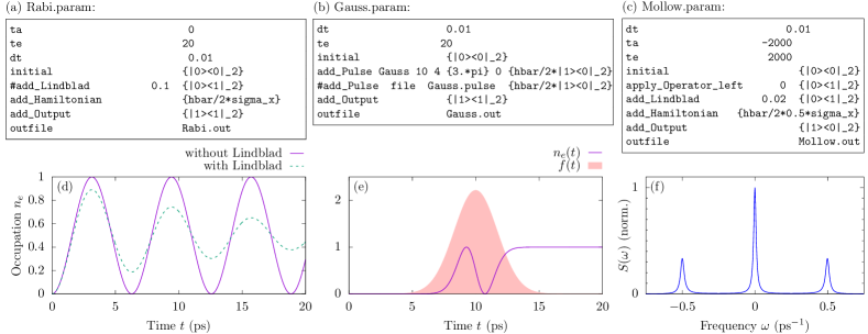
Figure 2: (a)-(c): Configuration files and (d)-(f): simulation results for examples of closed and Markovian quantum systems. (a) and (d): Rabi oscillations of a continuously driven two-level system with and without Lindbladian damping. (b) and (e): Two-level system driven with a Gaussian $3\pi$ pulse. (c) and (f): Extraction of first-order coherence and its Fourier transform for a driven two-level system, giving rise to a Mollow triplet in the emission spectrum.

For example, files containing pulse envelopes $f(t)$ are expected to contain times $t_{j}$ in the first column and real and imaginary parts of $f(t_{j})$ in the second and third column, respectively. Files for spectral densities $J(\omega)$, which describe how strongly Gaussian baths are coupled to the system at a given frequency $\omega$, have to contain two columns: the first containing frequencies $\omega_{j}$ and the second containing the (real) value of $J(\omega_{j})$, both in ps^-1.

Output files contain time points $t_{j}$ in the first column. For each observable specified using add_Output, the operator average $\langle A(t)\rangle=\textrm{Tr}(A\rho(t))$ is extracted and represented as two columns in the output file, corresponding to real and imaginary parts, respectively. Due to their size PT-MPOs are stored as binary files and may be split into several files each containing a block of at most $B$ PT-MPO matrices, where $B$ is specified by buffer_blocksize.

IV Examples

IV.1 Closed and Markovian quantum systems

We begin with a simple example for the usage of the ACE code, starting with a continuously driven closed two-level system without any environment. To this end, we run ACE Rabi.param with the configuration file shown in Fig. 2(a). There, the time grid is set to go from time ta=0 to te=20 ps in steps of dt=0.01 ps. The initial state (parameter initial) is set to the ground state $\bar{\rho}(0)=|0\rangle\langle 0|$ of a two-level system, which is specified as a matrix-valued expression. We consider resonant Rabi driving using the Hamiltonian $H_{S}=\frac{\hbar}{2}(1\textrm{ ps}^{-1})\sigma_{x}$, where we use the constant hbar to convert frequencies in ps^-1 to energies in meV. The observable we are interested in is the occupation $n_{e}(t)=\textrm{Tr}(|1\rangle\langle 1|\bar{\rho}(t))$. This is specified using add_Output, and the outfile parameter instructs to code to save this observable in the output file Rabi.out.

Optionally, we add radiative loss modeled by the Lindbladian $(0.1\textrm{ ps}^{-1})\mathcal{D}_{|0\rangle\langle 1|}[\bar{\rho}]$ with

$$\mathcal{D}_{\hat{A}}[\bar{\rho}]=\hat{A}\bar{\rho}\hat{A}^{\dagger}-\frac{1}{2}(\hat{A}^{\dagger}\hat{A}\bar{\rho}+\bar{\rho}\hat{A}^{\dagger}\hat{A}).$$ (11)

This term is commented out in the configuration file in Fig. 2(a), as all characters in a line after the symbol # are ignored. Thus, removing this symbol we simulate the corresponding Markovian open quantum system. The results with and without Lindblad term are depicted in Fig. 2(d) and show the expected (damped) Rabi oscillations.

More generally, quantum systems can be driven with pulses, i.e., with time-dependent system Hamiltonians $H_{S}(t)$. In Fig. 2(b) and (e), we demonstrate the simulation of a two-level system driven with a strong Gaussian pulse. Concretely, we apply a system Hamiltonian

$$H_{S}(t)=(f(t)\hat{d}+f^{*}(t)\hat{d}^{\dagger})$$ (12)

with a scalar function $f(t)$ and an operator $\hat{d}$ acting on the system Hilbert space. We choose a Gaussian pulse

$$f(t)= \frac{A}{\sqrt{2\pi}\sigma}e^{-\frac{1}{2}\frac{(t-t_{c})^{2}}{\sigma^{2}}}e^{-i(\delta/\hbar)t},$$ (13)

with pulse area $A=3\pi$, pulse center $t_{c}=10$ ps, standard deviation $\sigma=\tau_{\textrm{FWHM}}/(2\sqrt{2\ln 2})$ with pulse duration $\tau_{\textrm{FWHM}}=4$ ps, and detuning $\delta=0$ meV. Furthermore, we use the coupling operator $\hat{d}=(\hbar/2)|1\rangle\langle 0|$.

The time-dependent driving can be specified as indicated in Fig. 2(b), in one of two ways. Either one can use a predefined add_Pulse command. Here, Gauss takes parameters in the following order: $t_{c}$, $\tau_{\textrm{FWHM}}$, $A$, $\delta$, and $\hat{d}$. Alternatively, as in the out-commented line in Fig. 2(b), a pulse can be read from a file (here: file name Gauss.pulse) with three columns: time points $t_{j}$ and real and imaginary parts of $f(t_{j})$. The Hermitian conjugate part is added automatically. This makes it possible to create completely arbitrary pulse shapes.

Finally, sometimes not only the density matrix is of interest but also multi-time correlation functions. For example, the emission spectrum of a two-level system is related to the first-order coherences $g^{(1)}(t,\tau)=\langle\sigma^{+}(t+\tau)\sigma^{-}(t)\rangle$ by

$$S(\omega)=\textrm{Re}\int\limits_{0}^{\infty}d\tau\,\big{[}g^{(1)}(t,\tau)-g^{(1)}(t,\infty)\big{]}e^{-i\omega\tau}.$$ (14)

To evaluate the first-order coherences, we have to first propagate the system until it reaches a stationary state at time $t$, then apply the operator $\sigma^{-}=|0\rangle\langle 1|$ and propagate for another time $\tau$, where the observable $\sigma^{+}=|1\rangle\langle 0|$ is extracted. In Fig. 2(c), we depict the configuration file for simulating a continuously driven two-level system from time ta=-2000 ps to time te=2000 ps. At time $t=0$, the operator $|0\rangle\langle 1|$ is applied from the left onto the density matrix, which is instructed with the command apply_Operator_left, whose first argument is the time of application and the second argument is the operator to be applied. In Fig. 2(f), we present $S(\omega)$, which we obtain by Fourier transforming the second and third columns (real and imaginary parts) of the output file after cutting off all data in the output file prior to time $t$ and subtracting the stationary part according to Eq. (14). A Mollow triplet is observed with the side peaks at the Rabi frequency $\Omega=0.5$ ps^-1.

IV.2 Usage of the ACE algorithm

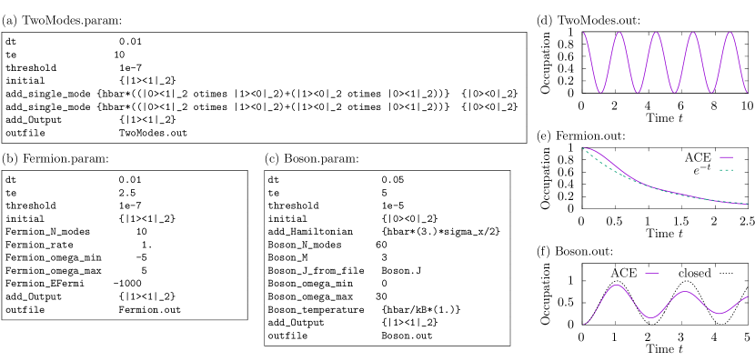
Figure 3: Configuration files [(a),(b), and (c)] and results [(d), (e), and (f)] of examples using ACE: (a) and (d): Two-level system coupled to two environment modes, which are specified explicitly. (b) and (e): Resonant level model with $N_{E}=10$ fermionic environment modes with Markov approximation $e^{-t}$ for reference. (c) and (f): Driven two-level system with and without spin-boson environment. The Ohmic spectral density is specified in file Boson.J.

Having described how closed and Markovian quantum systems can be simulated using the ACE code, we now turn to non-Markovian open quantum systems. As shown in Fig. 3, there are several ways to use the ACE algorithm [33] to construct PT-MPOs from the explicit microscopic Hamiltonians of a set of $N_{E}$ environment modes and to obtain the exact system dynamics up to an MPO compression error controlled by the threshold $\epsilon$ and Trotter error controlled by dt.

The first is to specify individual modes with the add_single_mode command, as depicted in Fig. 3(a). The two arguments are matrix-valued expressions for the mode Hamiltonian and for the initial state of the mode. Note that the mode Hamiltonian includes the coupling to the system and thus acts on the space $\mathcal{H}_{S}\otimes\mathcal{H}_{E}^{(k)}$, while the inital state is a density matrix acting on the mode Hilbert space $\mathcal{H}_{E}^{(k)}$ alone. In the example in Fig. 3(a), we couple a two-level system to two identical modes via Hamiltonians $H_{E}^{(k)}=\hbar g(\sigma^{-}c^{\dagger}_{k}+\sigma^{+}c_{k})$, where $\sigma^{\pm}$ excite and destroy excitations in the central two-level system and $c^{\dagger}_{k}$ and $c_{k}$ do the same for the $k$-th environment mode, which is also a two-level system. The coupling constant is set to $g=1$ (technically in ps^-1, but identified with a dimensionless value). The central two-level system is initially occupied while the environment modes are initially empty. The result is depicted in Fig. 3(d), where one observes coherent oscillations between the central two-level systems and the symmetric linear combination of the two environment modes.

Alternatively, for some frequently occuring environment models, the ACE code offers generators, which facilitate the convenient specification of a quasi-continuum of environment modes. In Fig. 3(b) and (c), we use the Fermion and Boson generators, respectively. Both require a series of similar commands starting with Fermion_ and Boson_, respectively. For example, ...N_modes defines the number of modes used for discretizing the continuum on a frequency interval defined by the limits ...omega_min and ...omega_max. In the bosonic case in Fig. 3(c), the parameter Boson_M determines the size of the truncated Hilbert space per bosonic mode. For both types of environments, the ...temperature can be set by the corresponding command. If not set explicitly, a default value of $T=0$ is taken. The specified value is assumed be given in units of Kelvin. An effectively dimensionless specification (typically denoted by $1/\beta$ in statistical physics) is achieved by mapping all energies to units of ps^-1, which we do in Fig. 3(c) by multiplying with $\hbar$ (in meV ps) and dividing by the Boltzmann constant $k_{B}$ (in meV/K). In the fermionic case in Fig. 3(b), the Fermi energy is specified by Ferion_E_Fermi.

The system-environment coupling operator $\hat{A}$ can be specified as matrix-valued expression using Fermion_SysOp and Boson_SysOp, respectively. The mode Hamiltonian is then set to

$$H_{E}^{(k)}= \sum_{k}\hbar\omega_{k}b^{\dagger}_{k}b_{k}+\sum_{k}\hbar g_{k}(\hat{A}b^{\dagger}_{k}+\hat{A}^{\dagger}b_{k}),$$ (15)

for the Boson generator and equivalent with boson operators replaced by fermion operators for the Fermion generator. This contains several often-used models: The default value for Fermion_SysOp is |0><1|_2, which corresponds to the resonant-level model describing a particle number conserving hopping processes. The default value for Boson_SysOp is |1><1|_2, the projection onto the excited state, which describes a spin-boson model for a two-level system. The Jaynes-Cummings model is obtained by setting Boson_SysOp to |0><1|_2. Note that for the Boson generator automatically subtracts the polaron shift or reorganization energy [see discussion of Eq. (9)]. If this is not desired, it can be switched off by the command Boson_subtract_polaron_shift false.

There are also several ways to specify the coupling constant to each of the bath modes. If the coupling to all modes is identical, one can provide the value of $g$ via Fermion_g. However, if the modes discretize a continuum, it is instructive to instead supply the rate $\Gamma$ expected in the Markov limit by Fermi’s Golden Rule. This is set by Fermion_rate in Fig. 3(b) and determines the coupling constants by $g=\sqrt{\Gamma(\omega_{\textrm{max}}-\omega_{\textrm{min}})/(2\pi N_{E})}$. Note that for any finite bandwidth $\omega_{\textrm{max}}-\omega_{\textrm{min}}$ the exact dynamics deviates from the Markovian dynamics—here $e^{-t}$—which is also shown in the results in Fig. 3(e).

When the system-environment coupling varies with frequency, one can instead supply a spectral density defined by $J(\omega)=\sum_{k}|g_{k}|^{2}\delta(\omega-\omega_{k})$. This is used in the the example of a spin-boson model in Fig. 3(c) and (f). In the configuration file in panel (c), the command Boson_J_from_file instructs the code to read the spectral density from the file Boson.J, in which we stored (frequency $\omega_{j}$ in the first column; value of $J(\omega_{j})$ in the second column) an ohmic spectral density $J(\omega)=0.2\,\omega\exp({-\omega/(3\textrm{ ps}^{-1})})$. The coupling to this bosonic environment results in damping of Rabi rotations as shown in Fig. 3(f).

IV.3 Selection of methods

Whenever single modes or a corresponding generator is provided (the ..._N_modes parameter set to a positive value), the default behavior of the code is to calculate the corresponding PT-MPO using the ACE algorithm of Ref. [33]. As discussed in the method section II the ACE code also supports the tree-like contraction scheme of Ref. [43], which is used when the command use_combine_tree true is found in the configuration file.

The methods utilizing the Gaussian property of the spin-boson model can be switched on by stating use_Gaussian true. They then process the same parameters as the Boson mode generator, such as the spectral density, temperature, minimum and maximum frequency defining the frequency range, and whether or not to subtract the polaron shift. The default Gaussian method is the one by Jørgensen and Pollock in Ref. [29]. The divide-and-conquer scheme of Ref. [40] is switched on by use_Gaussian_divide_and_conquer true. Periodic PT-MPOs, also derived in Ref. [40], are used when one sets use_Gaussian_periodic true.

The Gaussian methods allow for memory truncation, i.e. neglecting the bath correlation function beyond $n_{\textrm{mem}}=t_{\textrm{mem}}/\Delta t$ time steps. The memory time can be set in the configuration file by the parameter t_mem. Note that one should set the memory cut-off $n_{\textrm{mem}}$ to a power of two for the divide-and-conquer as well as for the periodic PT-MPO method. Generally, the computation time does not monotonically decrease when the memory time is reduced. This is likely due to the fact that a sudden jump to zero in the effective bath correlation function results in spurious long-range temporal correlations that increase the inner bond dimensions of the PT-MPOs. Heurestically, we suggest starting with a value of $t_{\textrm{mem}}$ which is about a factor 4 longer than the time scale on which the bath correlation function is found to drop to zero by visual inspection, and then varying the memory time to find an optimum in computation time.

All the PT-MPO-based methods are implemented within the ACE binary. Our framework further provides binaries QUAPI and TEMPO, which implement the path integral methods of Refs. [24, 25, 46] and Ref. [38], respectively. Both parse the same configuration file containing parameters of the Boson generator. Note that the memory consumption of QUAPI scales exponentially with the number of memory time steps $n_{\textrm{mem}}$, so the corresponding parameter should not exceed $\sim 12$, even for small, e.g., two-level systems.

IV.4 Convergence and fine tuning

Several convergence parameters exist that control the accuracy as well as the computation time of ACE and other PT-MPO techniques, such as the width of the time steps $\Delta t$ and MPO compression threshold $\epsilon$. As described above, these are set via parameters dt and threshold.

First, it should be noted that the compression error for a given threshold $\epsilon$ strongly depends on $\Delta t$ and thus comparing simulations with equal $\epsilon$ but different $\Delta t$ is not advised [33]. The maximal inner bond dimension of the respective final PT-MPOs tends to be a more stable indicator of the absolute compression error when the time steps $\Delta t$ are changed [33]. The inner bonds can be extracted from a process tensor file using the binary PTB_analyze -read_PT FILE.pt. Thus, to gauge the convergence with respect to both parameters, it is instructive to perform simulations where, for several values of the time step $\Delta t$, a series of values for the threshold spanning several orders of magnitude are tested and the impact on the observables is checked. Only after the compression error for fixed $\Delta t$ is understood, the Trotter error due to the finite time step $\Delta t$ can be checked reliably.

Moreover, if the environment modes in the ACE algorithm arise from discretizing a continuum, the number of modes $N_{E}$ (e.g., Boson_N_modes) and the bandwidth $\omega_{\textrm{max}}-\omega_{\textrm{min}}$ (e.g., Boson_omega_max and Boson_omega_min) constitute additional convergence parameters. For a given bandwidth, the optimal value of $N_{E}$ depends on the total propagation time $t_{e}-t_{a}$ via energy-time uncertainty. We recommend the choice $N_{E}=0.4(\omega_{\textrm{max}}-\omega_{\textrm{min}})(t_{e}-t_{a})$, where $0.4$ is a heuristic factor [33]. Note also that increasing the number of modes for a fixed bandwidth results in weaker coupling $g_{k}$ per mode. This again affects how the compression error on observables scales with the threshold $\epsilon$, and thus simulations with equal thresholds but different number of modes per bandwidth are not directly comparable.

For methods relying on the preselection approach for the PT-MPO combination, it is important to keep in mind that the corresponding compression can be significantly suboptimal, resulting in larger inner bond dimensions compared to other methods and also in more severe error accumulation. Especially in cases where very small time steps are used, simulations have been found to not converge with decreasing threshold [40, 43]. However, this can be mitigated by fine-tuning the compression.

To this end, several strategies have been explored: First, the divide-and-conquer and the periodic PT-MPO methods of Ref. [40] often profit from using a smaller threshold for singular value selection and backward sweep compared to the forward sweep. This is because the selection and backward sweep provides a less controlled truncation than the forward sweep, and the forward sweeps with coarser threshold partially remove spurious singular values introduced by the former. While the parameter threshold is used as a base value for the threshold, with parameters forward_threshold_ratio and backward_threshold_ratio one can set different thresholds for the two directions relative to the base value. Moreover, the parameter select_threshold_ratio specifically changes the threshold used in the preselection step. For example, in Ref. [40], we found backward_threshold_ratio 0.2 to result in reduced computation times for PT-MPOs describing the effects of phonons on semiconductor quantum dots.

For the tree-like ACE contraction scheme [43], we found it beneficial to employ a dynamically increasing threshold, where we keep the same thresholds for forward and backward sweeps within each pair of sweeps after a PT-MPO combination step but we gradually increase the threshold as the PT-MPO grows. Specifically, we start with a small threshold $\epsilon_{\textrm{min}}=\epsilon/r$ for the first PT-MPO combination and exponentially increase (linear interpolation of $\log\epsilon$) the threshold such that the compression after the final combination step occurs with threshold $\epsilon_{\textrm{max}}=\epsilon$. The factor $r$ is specified by threshold_range_factor. A value of $r=10$ to $r=100$ is often useful [43]. This fine-tuning strategy turns out to be useful also for Gaussian PT-MPO methods (see example in Sec. IV.7).

IV.5 Trotter Errors

The decomposition of the total propagator into system and envrionment parts in Eq. (4) has been derived using the asymmetric (first-order) Trotter decomposition $e^{\mathcal{L}\Delta t}=e^{\mathcal{L}_{E}\Delta t}e^{\mathcal{L}_{S}\Delta t}+\mathcal{O}(\Delta t^{2})$ in Eq. (3). The Trotter error can be reduced by using instead the symmetric (second order) Trotter decomposition $e^{\mathcal{L}\Delta t}=e^{\mathcal{L}_{S}\Delta t/2}e^{\mathcal{L}_{E}\Delta t}e^{\mathcal{L}_{S}\Delta t/2}+\mathcal{O}(\Delta t^{3})$. The use of the symmetric Trotter decomposition is now in fact the default behavior setting in our code.

However, for simulations with more than one PT-MPO with mutually non-communiting interaction Hamiltonians, we suggest an alternative decomposition, where the order of applying the PT-MPO matrices (with respect to outer index multiplication) alternates. Here, the understanding of PT-MPO matrices as compressed environment propagators is useful [30]. For example, if there are two environment propagators $e^{\mathcal{L}_{E}^{(1)}\Delta t}$ and $e^{\mathcal{L}_{E}^{(2)}\Delta t}$ in addition to the system propagator $e^{\mathcal{L}_{S}\Delta t}$, the propagation over two time steps is given by

$$e^{\mathcal{L}_{S}\Delta t}e^{\mathcal{L}_{E}^{(1)}\Delta t}e^{\mathcal{L}_{E}^{(2)}\Delta t}e^{\mathcal{L}_{E}^{(2)}\Delta t}e^{\mathcal{L}_{E}^{(1)}\Delta t}e^{\mathcal{L}_{S}\Delta t},$$ (16)

which describes a symmetric Trotter decomposition of the joint environment propagator over two time steps

$$e^{(\mathcal{L}_{E}^{(1)}+\mathcal{L}_{E}^{(2)})(2\Delta t)}=e^{\mathcal{L}_{E}^{(1)}\Delta t}e^{\mathcal{L}_{E}^{(2)}(2\Delta t)}e^{\mathcal{L}_{E}^{(1)}\Delta t}+\mathcal{O}(\Delta t^{3})$$ (17)

followed by a symmetric Trotter decomposition between system and the joint environment

$$e^{(\mathcal{L}_{S}+\mathcal{L}_{E}^{(1)}+\mathcal{L}_{E}^{(2)})(2\Delta t)}$$

$$=e^{\mathcal{L}_{S}\Delta t}e^{(\mathcal{L}_{E}^{(1)}+\mathcal{L}_{E}^{(2)})(2\Delta t)}e^{\mathcal{L}_{S}\Delta t}+\mathcal{O}(\Delta t^{3}).$$ (18)

This feature is turned on in the code on by setting the parameter propagate_alternate true, which overrides the use of the symmetric Trotter decomposition. Alternating the propagation order can lead to zigzagging behavior in the output, as observables at odd time steps have a larger Trotter error order than at even time steps. One should then keep only the values at even time steps (counting from zero). The difference between odd and even time steps can be used as an indicator for the Trotter error.

IV.6 Example: Composite system of QD and microcavity

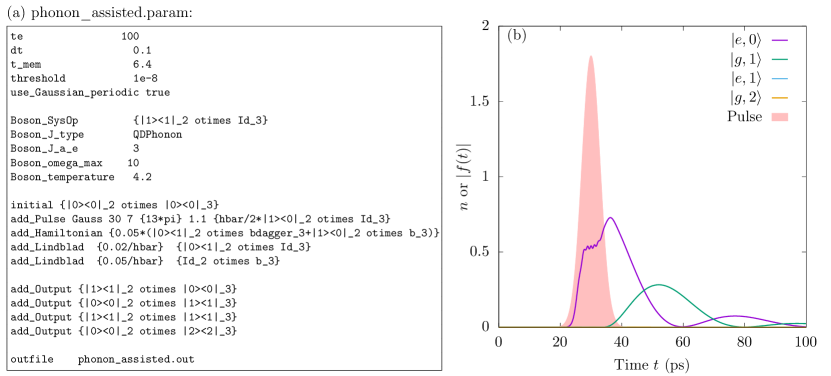
Figure 4: (a) Configuration file and (b) simulation results for phonon-assisted single-photon generation using a QD strongly coupled to an optical microcavity.

We now provide further examples to demonstrate some of the features mentioned previously. First, we consider a bipartite open quantum system, namely a semiconductor QD strongly coupled to longitudinal acoustic phonons as well as strongly coupled to an optical single-mode microcavity. The QD and the cavity are treated as part of the system. The phonon environment only couples to the QD part of the system. For semiconductor QDs, the coupling between electronic excitations and phonons can be derived from microscopic considerations [20]. In particular, assuming infinite-potential confinement along the growth direction and parabolic confinement in the in-plane directions, the electron-phonon coupling gives rise to a spin-boson model with spectral density

$$J(\omega)= \frac{\omega^{3}}{4\pi^{2}\rho\hbar c_{s}^{5}}\bigg{(}D_{e}e^{-\omega^{2}a_{e}^{2}/(4c_{s}^{2})}-D_{h}e^{-\omega^{2}a_{h}^{2}/(4c_{s}^{2})}\bigg{)}^{2},$$ (19)

where, for a QD in a GaAs matrix, the mass density is $\rho=5370$ kg/m³, the speed of sound is $c_{s}=5110$ m/s, and the electron and hole deformation potential constants are $D_{e}=7.0$ eV and $D_{h}=-3.5$ eV, respectively [20]. The lengths $a_{e}$ and $a_{h}$ are the electron and hole radii, respectively.

Because of the importance of QDs for quantum technology, we have implemented as a convenience option the specification of the spectral density in Eq. (19). As show in the configuration file in Fig. 4(a), this spectral density is chosen by setting Boson_J_type QDPhonon. The electron and hole radii can be set by Boson_J_a_e and Boson_J_a_h, respectively. If not set explicitly, $a_{e}$ has the value 4 nm and $a_{h}=a_{e}/1.15$. Moreover in Fig. 4(a) we set use_Gaussian_periodic true to generate a periodic PT-MPO. This requires a memory cutoff $n_{\textrm{mem}}$ which is a power of 2 times the time step $\Delta t=0.1$ ps, for which we set the parameter t_mem to 6.4 ps.

The concrete situation modeled in Fig. 4 is phonon-assisted state preparation for a QD strongly coupled to a microcavity, reproducing the example in Ref. [47]. There, the coupled system is driven by a blue-detuned (1.1 meV with respect to the two-level transition energy) Gaussian laser pulse. The cavity mode is on resonance with the two-level system. The QD-cavity coupling has a strength of $\hbar g=0.05$ meV, the cavity is lossy with loss rate $\kappa=0.05\textrm{ meV}/\hbar$, and two-level excitations decay radiatively with loss rate $\gamma=0.02\textrm{ meV}/\hbar$.

Note that the system initial state, Hamiltonians (pulses), Lindblandians, observables, and the system-environment coupling operator Boson_SysOp all act on the 6-dimensional composite system Hilbert space containing both QD and the truncated cavity mode. However, because the system-environment coupling operator is highly degenerate—which is automatically identified by the code—the PT-MPO calculation is only as difficult as that for an isolated two-level system.

The dynamics depicted in Fig. 4(b) can be understood in terms of adiabatic undressing [54]: The strong pulse leads to laser-dressing of states, such that (i) phonon-assisted transitions between dressed states are possible and lead to fast thermalization towards the lower dressed state, and (ii) the lower dressed states adiabatically evolves into the excited state as the pulse vanishes. A corresponding jump in the occupations of state $|e,0\rangle$ (excited states with zero photons in the cavity) is observed at the end of the pulse. The excitation is then transfered to the cavity via the QD-cavity coupling and then out-coupled from the cavity via cavity losses. Moreover, during the pulse, the dressing detunes the QD from the cavity frequency, which suppresses emission during the pulse and thereby reduces reexcitation. Because the laser is also off-resonant from the cavity, the phonon-assisted scheme combines several important features of single-photon generation: high single-photon purity, seperability of emitted photons from stray laser photons, and relatively high brightness. Because of these advantages, the phonon-assisted scheme is used in practical implementations of single-photon sources [55].

IV.7 Example: Photon coincidences from superradiant QDs

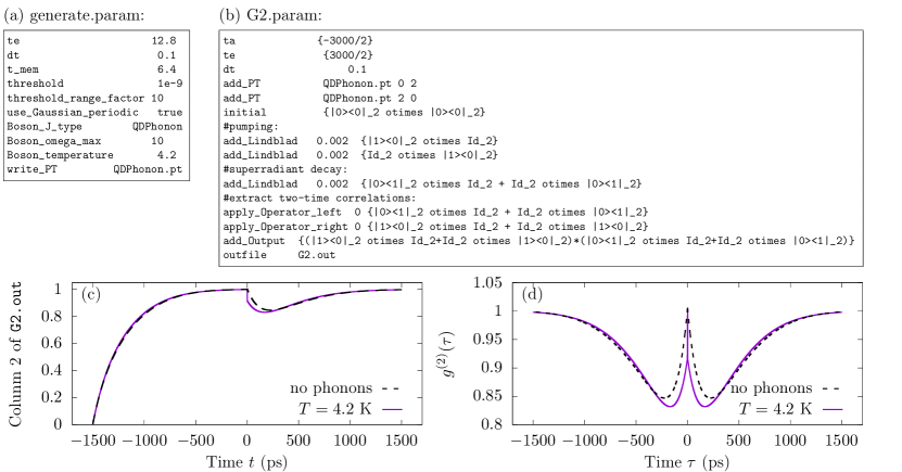
Figure 5: Configuration files for (a) PT-MPO generation and (b) simulation of photon coincidences from two incoherently driven superradiant quantum strongly coupled to local phonon baths. (c) Generated output with and without accounting for phonons. (d) Photon coincidences.

Our final example illustrates the use of multiple PT-MPOs at the same time. Motivated by recent experiments, which demonstrated cooperative emission from indistinguishable QDs [56, 57, 58, 59], we consider two QDs each coupled to a local non-Markovian phonon bath and both QDs coherently coupled to the electromagnetic environment.

Assuming a flat spectral density of the eletromagnetic environment, the latter can be described by a Lindblad term for the joint radiative decay [60, 35]. If the QDs have identical energies, the radiative decay is enhanced with respect to the emission from individual or distinguishable QDs, which is described by Lindbald terms involving the symmetric linear combination of dipole operators [4] $2\kappa\mathcal{D}_{\sigma^{-}_{S}}[\bar{\rho}]$, where

$$\sigma^{\pm}_{S}=\frac{1}{\sqrt{2}}(\sigma^{\pm}_{1}+\sigma^{\pm}_{2})$$ (20)

and $\kappa$ is the radiative decay of a single QD. We further assume the QDs to be independently pumped with a pump rate $\gamma_{p}$, which is described by Lindbladians $\gamma_{p}\mathcal{D}_{\sigma_{1}^{+}}[\bar{\rho}]+\gamma_{p}\mathcal{D}_{\sigma_{2}^{+}}[\bar{\rho}]$. Here, we set $\kappa=\gamma_{p}=1/(0.5\textrm{ ns})$.

To reveal collective effects in few-emitter systems, one often measures photon coincidences [56, 57, 58]

$$g^{(2)}(t,\tau)= \frac{G^{(2)}(t,\tau)}{I(t)I(t+\tau)},$$ (21)

where $I(t)=\langle\sigma^{+}_{S}(t)\sigma^{-}_{S}(t)\rangle$ is the intensity and

$$G^{(2)}(t,\tau)=\langle\sigma^{+}_{S}(t)\sigma^{+}(t+\tau)\sigma^{-}(t+\tau)\sigma^{-}(t)\rangle$$

$$=\textrm{Tr}\big{[}\big{(}\sigma^{+}(t+\tau)\sigma^{-}_{S}(t+\tau)\big{)}\big{(}\sigma^{-}_{S}(t)\rho(0)\sigma^{+}_{S}(t)\big{)}\big{]}$$ (22)

are the unnormalized coincidences. From the last line of Eq. (22), it is clear that $G^{(2)}$ can be obtained by propagating the open quantum system over a time $t$, then applying operator $\sigma^{-}_{S}$ from the left and $\sigma^{+}_{S}$ from the right, propagating further over time $\tau$, and finally evaluating the observable $\sigma^{+}\sigma^{-}$. This is precisely how we evaluate $G^{(2)}$ using the ACE code with the configuration file in Fig. 5(b), where we chose $t=0$.

Note that of the output, which is shown in Fig. 5(c), only the data points at strictly positive times $\tau>0$ are related to $G^{(2)}$ while data points at previous time steps describe the evolution of the intensity $I(t)$. Therefore, in Fig. 5(d), we mirror the results to also plot coincidences for negative delay times $\tau$ and zoom into the relevant range.

To account for phonon effects, we add two PT-MPOs to the simulation. This is done using the add_PT command, whose first argument is the name of the corresponding PT-MPO file, while the second and third arguments are optional parameters that denote whether the outer bonds of the PT-MPOs shall be temporarily (no change to file occurs) extended to support a larger composite system Hilbert space. Concretely, outer bonds calculated for a Hilbert space $\mathcal{H}^{(0)}_{S}$ are extended to support a composite space $\mathcal{H}_{\textrm{left}}\otimes\mathcal{H}^{(0)}_{S}\otimes\mathcal{H}_{\textrm{right}}$, where the second argument of the add_PT command denotes the dimension of $\mathcal{H}_{\textrm{left}}$ and the third argument is the dimension of $\mathcal{H}_{\textrm{right}}$. Hence, the first line in Fig. 5(b) containing add_PT indicates the PT-MPO that acts on the first QD and the next line describes the PT-MPO acting of the second QD.

Here, we use the same PT-MPO for both QDs, which is precalculated using the configuration file in Fig. 5(a). Again, we calculate a periodic PT-MPO and employ fine-tuning using the threshold range factor $r=10$ to slightly reduce the bond dimension. The command write_PT instructs the ACE code to write the calculated PT-MPO to the corresponding file. Generally, more than one PT-MPO file may be created, whose names start with the provided name. This is done to facilitate buffering, i.e. reading and writing from and to files. For example, a PT-MPO may be split up into several files each containing $B$ blocks of the PT-MPO using the command buffer_blocksize followed by the number $B$. This is useful when the full PT-MPO does not fit into working memory. Instead of add_PT, one can also load PT-MPOs using initial_PT. The difference is that the latter can only use at most one PT-MPO and potentially modifies it. For example, using initial_PT, combined with add_single_mode, and write_PT modifies an existing PT-MPO to include the effects of another single environment mode.

The explanation of the physics of the results in Fig. 5(d) follows along the lines of the analysis in Refs. [4, 36, 35]. First, photon coincidences without phonons can be derived analytically [4]. The exact dynamics and the value of $g^{(2)}(\tau=0)$ depend on the details, such as the ratio between pump strength and radiative decay. In any case, one observes a peak with a value of $g^{(2)}(\tau=0)$ significantly larger than 0.5, which is the limit for photon coincidences from distinguishable, uncorrelated emitters. The excess $g^{(2)}$ is directly related to inter-emitter coherences. Second, when a two-level system subject to a spin-boson interaction is not driven (no Hamiltonian term), one obtains an independent-boson model, which can be solved analytically [7]. For an independent-boson model with super-Ohmic spectral density, coherences initially drop but then remain constant. This behavior of the two-level system also translates to inter-emitter coherences of QDs coupled to two phonon baths [36], where phonons are found to also result in an initial fast drop in $g^{(2)}$ but after a few ps the dynamics with phonons decays and restores in parallel with the phonon-free case.

This example demonstrates how the ACE code can solve a multi-partite, non-Markovian multi-environment, and multi-scale problem in a numerically complete way with only few lines in the configuration files and no further programming required.

V Summary

We have described the ACE code [44], which is a versatile solver for non-Markovian open quantum systems based on PT-MPOs. The concrete physical problem is specified in configuration files. The corresponding commands and parameters are discussed on a series of examples from simple closed systems to multi-partite multi-environment problems.

The ACE code implements several methods to calculate PT-MPOs and allows PT-MPOs to be stored in files, manipulated, combined with other PT-MPOs, and read again to efficiently scan simulation results for different time-dependent system Hamiltonians. When the environment is of the form of a Gaussian spin-boson model, one can use the algorithm by Jørgensen and Pollock [29], the divide-and-conquer algorithm of Ref. [40], or periodic PT-MPOs. If the environment is more generally composed of independent modes, the ACE algorithm of Ref. [33] as well as an enhanced version with a tree-like combination scheme [43] is available. Moreover, it is possible to compose open quantum system and use several PT-MPOs to describe environment influences. This makes the code extremely versatile, and it demonstrates the core idea for the development of a universal numerically exact solver for networks of non-Markovian open quantum systems based on PT-MPOs.

A current limitation of the code is the size of the open quantum system network because the propagation of a multi-partite system with several PT-MPOs by the analog of Eq. (7) involves the multiplication of matrices, whose dimensions are the products of the individual system Liouville space dimensions and the inner bonds of the PT-MPOs. Future work will be directed towards tackling the exponential scaling with the number of constituent parts of the quantum networks.

Appendix A Summary of commands and arguments

Command	Arguments	Comments
Basic controls:
dt	float	Time step $\Delta t$ (unit: ps, default value: 0.01)
ta	float	Initial time of simulation $t_{a}$ (unit: ps, default value: 0)
te	float	Final time of simulation $t_{e}$ (unit: ps, default value: 10)
outfile	string	Name of output file to be created
use_symmetric_Trotter	bool	Switches on second order (as opposed to first-order) Trotter splittings between system propagators and PT-MPO matrices (default value: true).
propagate_alternate	bool	Switches on alternating order for system and envrionment propagators for multi-environment simulations (overrides use_symmetric_Trotter; default value: false).
System parameters:
initial	matrix	Initial system density matrix.
add_Hamiltonian	matrix	Adds [argument] to the (time-constant) system Hamiltonian.
add_Pulse	string […]	Adds time-dependent part of system Hamiltonian. The first arguments determines the type of pulse, e.g., file for reading pulses from a file or Gauss for using a predefined Gaussian pulse. The remaining parameters depend on this choice [see example in Fig. 2(b)].
add_Lindblad	float matrix	Adds a Lindblad term to the free system propagator. The first argument is the rate in ps-1, the second argument is the collapse operator.
apply_Operator_left	float matrix	Multiplies the system density matrix at time [first argument] with an operator [second argument] from the left, e.g., to extract multitime correlation functions.
apply_Operator_right	float matrix	Multiplies the system density matrix at time [first argument] with an operator [second argument] from the right.
add_Output	matrix	Specifies an observable [argument] to be extracted from the reduced system density matrix. Every occurrence of add_Output results in the addition of two columns to the outfile, corresponding to real and imaginary parts of the observable.
Handling of PT-MPOs and compression:
threshold	float	Base MPO compression threshold; relative to largest SVD (default value: 0=no truncation)
t_mem	float	Memory time used for memory truncation $t_{\textrm{mem}}$ (ps)
n_mem	float	Memory cut-off (number of steps) used for memory truncation. Overrides t_mem.
forward_threshold_ratio	float	When sweeping in forward direction (from $t=t_{a}$ to $t=t_{e}$), the compression threshold is multiplied by this value (default value: 1).
backward_threshold_ratio	float	When sweeping in backward direction (from $t=t_{e}$ to $t=t_{a}$), the compression threshold is multiplied by this value (default value: 1).
select_threshold_ratio	float	When using preselection for PT-MPO combination, the compression threshold is multiplied by this value (default value: 1). Note that forward_threshold_ratio or backward_threshold_ratio also apply depending on the sweep direction.
final_sweep_n	int	[argument] additional pairs of line sweeps are performed at the end of the PT-MPO generation (default value: 0)
final_sweep_threshold	float	Explicitly sets the threshold for final sweeps (default value: value of threshold)
add_PT	string [int] [int]	Read (read-only) PT-MPO from file (first argument = file name). Optionally, extend outer bond dimensions by a Hilbert space of dimension=[second argument] to the left and dimension=[third argument] to the right.
initial_PT	string	Read and modify PT-MPO from file [argument]
write_PT	string	Write generated or modified PT-MPO to file [argument]
buffer_blocksize	int	Break up PT-MPO in blocks of size [argument]

Table 2: List of commands that can be specified in configuration files. For more commands for PT-MPO generation see Tab. 3. The second column lists the type and order of arguments of the respective command, which are described in the third column. Multiple arguments are separated by white spaces. Types are either text strings (string; must not contain whitespaces), floating point numbers (float), integers (int), matrix-valued expressions (matrix) as described in Sec. III.2, or boolean values (bool). Floating point numbers can also be specified as 1x1 matrix-valued expressions. Arguments in square brackets are optional.

Command	Arguments	Comments
PT-MPO method selection:
use_combine_tree	bool	Selects the tree-like contraction scheme for ACE in Ref. [43] (default value: false)
use_Gaussian	bool	Selects the algorithm by Jørgensen and Pollock [29] for the generalized spin-boson model. All Gaussian methods use parameters of the Boson_... generator (default value: false)
use_Gaussian_divide_and_conquer	bool	Selects the divide-and-conquer scheme of Ref. [40] for the generalized spin-boson model. (default value: false)
use_Gaussian_periodic	bool	Selects the periodic PT-MPO scheme of Ref. [40] for the generalized spin-boson model. Note that the memory time t_mem should be specified (default value: false)
Environment mode specification:
add_single_mode	matrix matrix	A single environment mode is specified. The first argument contains the environment Hamiltonian $H_{E}$ on the Hilbert space $\mathcal{H}_{S}\otimes\mathcal{H}_{\textrm{mode}}$. The second argument is the initial density matrix of the mode on $\mathcal{H}_{\textrm{mode}}$.
add_single_mode_from_file	string matrix	A single environment mode is added, where the environment mode propagator is specified in the file [first argument]. The file has the format of a usual configuration file, where add_Hamiltonian, add_Pulse, add_Lindblad, and apply_Operator_... are interpreted as acting on the composite Hilbert space $\mathcal{H}_{S}\otimes\mathcal{H}_{\textrm{mode}}$. The second argument is the initial mode density matrix.
Boson generator:
Boson_N_modes	int	Number of modes used to discretize the bosonic continuum. Ignored if any of the Gaussian methods are used.
Boson_M	int	Hilbert space dimension per mode. Ignored if any of the Gaussian methods are used.
Boson_SysOp	matrix	System operator in the system-environment interaction. See discussion of Eq. (15).
Boson_J_from_file	string	Coupling constants are defined by discretizing a spectral density provided in file [argument]. See discussion of Fig. 3(c).
Boson_J_type	string […]	Use a predefined spectral density. See discussion of Fig. 4(a).
Boson_g	float	Coupling constant to all modes is set equal to [argument] (units: ps-1). See discussion of Fig. 3.
Boson_rate	float	Coupling constant to all modes is set by matching the Markovian rate to [argument] (units: ps-1). See discussion of Fig. 3.
Boson_omega_min	float	Lower frequency limit of mode continuum (unit: ps-1; default value=0).
Boson_omega_max	float	Upper frequency limit of mode continuum (unit: ps-1; default value=0).
Boson_temperature	float	Sets the initial state of the bath as a thermal state with temperature [first argument] (units: K; default value: 0).
Boson_subtract_polaron_shift	bool	Absorbs the polaron shift into a redefinition of system energies (default value: true).
Fermion generator:
Fermion_...	…	Same as the corresponding commands for the Boson generator, except for the following commands.
Fermion_EFermi	float	Initial Fermi energy (units: meV; default value: -106 meV)

Table 3: More control commands for PT-MPO generation. Same format as Tab. 2.

In Tab. 2, we provide a summary of commands to control the propagation of the open quantum system, the system propagator, and the handling of PT-MPOs. Further commands for controlling PT-MPO generation are listed in Tab. 3.

References

- Kundu, Dani, and Makri [2022] S. Kundu, R. Dani, and N. Makri, “Tight inner ring architecture and quantum motion of nuclei enable efficient energy transfer in bacterial light harvesting,” Science Advances 8, eadd0023 (2022).
- Tamascelli et al. [2019] D. Tamascelli, A. Smirne, J. Lim, S. F. Huelga, and M. B. Plenio, “Efficient simulation of finite-temperature open quantum systems,” Phys. Rev. Lett. 123, 090402 (2019).
- Carmichael [1993] H. Carmichael, An Open Systems Approach to Quantum Optics (Springer Berlin Heidelberg, 1993).
- Cygorek et al. [2023] M. Cygorek, E. D. Scerri, T. S. Santana, Z. X. Koong, B. D. Gerardot, and E. M. Gauger, “Signatures of cooperative emission in photon coincidence: Superradiance versus measurement-induced cooperativity,” Phys. Rev. A 107, 023718 (2023).
- Reiter, Kuhn, and Axt [2019] D. E. Reiter, T. Kuhn, and V. M. Axt, “Distinctive characteristics of carrier-phonon interactions in optically driven semiconductor quantum dots,” Advances in Physics: X 4, 1655478 (2019).
- Pollock et al. [2018] F. A. Pollock, C. Rodríguez-Rosario, T. Frauenheim, M. Paternostro, and K. Modi, “Non-markovian quantum processes: Complete framework and efficient characterization,” Phys. Rev. A 97, 012127 (2018).
- Breuer and Petruccione [2002] H.-P. Breuer and F. Petruccione, The Theory of Open Quantum Systems (Oxford University Press, Oxford, 2002).
- Lindblad [1976] G. Lindblad, “On the generators of quantum dynamical semigroups,” Communications in Mathematical Physics 48, 119–130 (1976).
- Press et al. [1992] W. H. Press, S. A. Teukolsky, W. T. Vetterling, and B. P. Flannery, Numerical Recipes in C, 2nd ed. (Cambridge University Press, Cambridge, USA, 1992).
- Johansson, Nation, and Nori [2012] J. Johansson, P. Nation, and F. Nori, “QuTiP: An open-source Python framework for the dynamics of open quantum systems,” Computer Physics Communications 183, 1760–1772 (2012).
- Krämer et al. [2018] S. Krämer, D. Plankensteiner, L. Ostermann, and H. Ritsch, “Quantumoptics. jl: A julia framework for simulating open quantum systems,” Computer Physics Communications 227, 109–116 (2018).
- de Vega and Alonso [2017] I. de Vega and D. Alonso, “Dynamics of non-markovian open quantum systems,” Rev. Mod. Phys. 89, 015001 (2017).
- Brenes et al. [2020] M. Brenes, J. J. Mendoza-Arenas, A. Purkayastha, M. T. Mitchison, S. R. Clark, and J. Goold, “Tensor-network method to simulate strongly interacting quantum thermal machines,” Phys. Rev. X 10, 031040 (2020).
- Chin et al. [2010] A. W. Chin, A. Datta, F. Caruso, S. F. Huelga, and M. B. Plenio, “Noise-assisted energy transfer in quantum networks and light-harvesting complexes,” New J. Phys. 12, 065002 (2010).
- Schollwöck [2011] U. Schollwöck, “The density-matrix renormalization group in the age of matrix product states,” Ann. Phys. (N.Y.) 326, 96 – 192 (2011).
- Rossi and Kuhn [2002] F. Rossi and T. Kuhn, “Theory of ultrafast phenomena in photoexcited semiconductors,” Rev. Mod. Phys. 74, 895–950 (2002).
- Cygorek et al. [2017a] M. Cygorek, F. Ungar, P. I. Tamborenea, and V. M. Axt, “Influence of nonmagnetic impurity scattering on spin dynamics in diluted magnetic semiconductors,” Phys. Rev. B 95, 045204 (2017a).
- Axt and Stahl [1994] V. M. Axt and A. Stahl, “A dynamics-controlled truncation scheme for the hierarchy of density matrices in semiconductor optics,” Zeitschrift für Physik B Condensed Matter 93, 195–204 (1994).
- Thomas et al. [2019] J. O. Thomas, B. Limburg, J. K. Sowa, K. Willick, J. Baugh, G. A. D. Briggs, E. M. Gauger, H. L. Anderson, and J. A. Mol, “Understanding resonant charge transport through weakly coupled single-molecule junctions,” Nature Communications 10, 4628 (2019).
- Krummheuer et al. [2005] B. Krummheuer, V. M. Axt, T. Kuhn, I. D’Amico, and F. Rossi, “Pure dephasing and phonon dynamics in gaas- and gan-based quantum dot structures: Interplay between material parameters and geometry,” Phys. Rev. B 71, 235329 (2005).
- Feynman and Vernon [1963] R. Feynman and F. Vernon, “The theory of a general quantum system interacting with a linear dissipative system,” Ann. Phys. (N.Y.) 24, 118 – 173 (1963).
- Tanimura and Kubo [1989] Y. Tanimura and R. Kubo, “Time evolution of a quantum system in contact with a nearly Gaussian-Markoffian noise bath,” J. Phys. Soc. Jpn. 58, 101–114 (1989).
- Tanimura [1990] Y. Tanimura, “Nonperturbative expansion method for a quantum system coupled to a harmonic-oscillator bath,” Phys. Rev. A 41, 6676–6687 (1990).
- Makri and Makarov [1995a] N. Makri and D. E. Makarov, “Tensor propagator for iterative quantum time evolution of reduced density matrices. I. Theory,” J. Chem. Phys. 102, 4600–4610 (1995a).
- Makri and Makarov [1995b] N. Makri and D. E. Makarov, “Tensor propagator for iterative quantum time evolution of reduced density matrices. II. Numerical methodology,” J. Chem. Phys. 102, 4611–4618 (1995b).
- Makri [2020] N. Makri, “Small matrix disentanglement of the path integral: Overcoming the exponential tensor scaling with memory length,” The Journal of Chemical Physics 152, 041104 (2020).
- Huang et al. [2023] Y.-T. Huang, P.-C. Kuo, N. Lambert, M. Cirio, S. Cross, S.-L. Yang, F. Nori, and Y.-N. Chen, “An efficient julia framework for hierarchical equations of motion in open quantum systems,” Communications Physics 6, 313 (2023).
- Kundu and Makri [2023] S. Kundu and N. Makri, “Pathsum: A c++ and fortran suite of fully quantum mechanical real-time path integral methods for (multi-)system + bath dynamics,” J. Chem. Phys. 158 (2023).
- Jørgensen and Pollock [2019] M. R. Jørgensen and F. A. Pollock, “Exploiting the causal tensor network structure of quantum processes to efficiently simulate non-markovian path integrals,” Phys. Rev. Lett. 123, 240602 (2019).
- Cygorek and Gauger [2024] M. Cygorek and E. M. Gauger, “Understanding and utilizing the inner bonds of process tensors,” (2024), arXiv:2404.01287 [quant-ph] .
- Fux et al. [2021] G. E. Fux, E. P. Butler, P. R. Eastham, B. W. Lovett, and J. Keeling, “Efficient exploration of hamiltonian parameter space for optimal control of non-markovian open quantum systems,” Phys. Rev. Lett. 126, 200401 (2021).
- Cosacchi et al. [2021a] M. Cosacchi, T. Seidelmann, M. Cygorek, A. Vagov, D. E. Reiter, and V. M. Axt, “Accuracy of the quantum regression theorem for photon emission from a quantum dot,” Phys. Rev. Lett. 127, 100402 (2021a).
- Cygorek et al. [2022] M. Cygorek, M. Cosacchi, A. Vagov, V. M. Axt, B. W. Lovett, J. Keeling, and E. M. Gauger, “Simulation of open quantum systems by automated compression of arbitrary environments,” Nat. Phys. 18, 662–668 (2022).
- Gribben et al. [2022] D. Gribben, D. M. Rouse, J. Iles-Smith, A. Strathearn, H. Maguire, P. Kirton, A. Nazir, E. M. Gauger, and B. W. Lovett, “Exact dynamics of nonadditive environments in non-markovian open quantum systems,” PRX Quantum 3, 010321 (2022).
- Wiercinski, Cygorek, and Gauger [2024] J. Wiercinski, M. Cygorek, and E. M. Gauger, “The role of polaron dressing in superradiant emission dynamics,” (2024), arXiv:2403.05533 [quant-ph] .
- Wiercinski, Gauger, and Cygorek [2023] J. Wiercinski, E. M. Gauger, and M. Cygorek, “Phonon coupling versus pure dephasing in the photon statistics of cooperative emitters,” Phys. Rev. Res. 5, 013176 (2023).
- Fux et al. [2023] G. E. Fux, D. Kilda, B. W. Lovett, and J. Keeling, “Tensor network simulation of chains of non-markovian open quantum systems,” Phys. Rev. Res. 5, 033078 (2023).
- Strathearn et al. [2018] A. Strathearn, P. Kirton, D. Kilda, J. Keeling, and B. W. Lovett, “Efficient non-markovian quantum dynamics using time-evolving matrix product operators,” Nat. Commun. 9, 3322 (2018).
- The TEMPO collaboration [2020] The TEMPO collaboration, “OQuPy: A Python 3 package to efficiently compute non-Markovian open quantum systems.” (2020), DOI: 10.5281/zenodo.4428316.
- Cygorek et al. [2024a] M. Cygorek, J. Keeling, B. W. Lovett, and E. M. Gauger, “Sublinear scaling in non-markovian open quantum systems simulations,” Phys. Rev. X 14, 011010 (2024a).
- Link, Tu, and Strunz [2024] V. Link, H.-H. Tu, and W. T. Strunz, “Open quantum system dynamics from infinite tensor network contraction,” Phys. Rev. Lett. 132, 200403 (2024).
- Ye and Chan [2021] E. Ye and G. K.-L. Chan, “Constructing tensor network influence functionals for general quantum dynamics,” The Journal of Chemical Physics 155, 044104 (2021).
- Cygorek et al. [2024b] M. Cygorek, B. W. Lovett, J. Keeling, and E. M. Gauger, “Tree-like process tensor contraction for automated compression of environments,” (2024b), arXiv:2405.16548 [quant-ph] .
- Cygorek [2024] M. Cygorek, “Ace code release v1.2.0,” (2024), DOI: 10.5281/zenodo.11383867.
- Note [1] Feynman and Vernon assume in Ref. [21] that the system of interest couples to the bath via the position coordinate. This corresponds to a diagonalizable coupling as, e.g., in the spin-boson model, but does not capture more general couplings via a sum of terms, where the system operators cannot be simultaneously diagonalized. In the latter case, the influence functional must be able to induce transitions between states, which corresponds to entries with index combinations for . If the coupling is diagonal, i.e. , then a single index per time step is sufficient, and one obtains the original form of the Feynman-Vernon influence functional in Ref. [21].
- Cygorek et al. [2017b] M. Cygorek, A. M. Barth, F. Ungar, A. Vagov, and V. M. Axt, “Nonlinear cavity feeding and unconventional photon statistics in solid-state cavity qed revealed by many-level real-time path-integral calculations,” Phys. Rev. B 96, 201201 (2017b).
- Cosacchi et al. [2019] M. Cosacchi, F. Ungar, M. Cygorek, A. Vagov, and V. M. Axt, “Emission-frequency separated high quality single-photon sources enabled by phonons,” Phys. Rev. Lett. 123, 017403 (2019).
- Cosacchi et al. [2020] M. Cosacchi, J. Wiercinski, T. Seidelmann, M. Cygorek, A. Vagov, D. E. Reiter, and V. M. Axt, “On-demand generation of higher-order fock states in quantum-dot–cavity systems,” Phys. Rev. Research 2, 033489 (2020).
- Cosacchi et al. [2021b] M. Cosacchi, T. Seidelmann, J. Wiercinski, M. Cygorek, A. Vagov, D. E. Reiter, and V. M. Axt, “Schrödinger cat states in quantum-dot-cavity systems,” Phys. Rev. Res. 3, 023088 (2021b).
- Seidelmann et al. [2019] T. Seidelmann, F. Ungar, A. M. Barth, A. Vagov, V. M. Axt, M. Cygorek, and T. Kuhn, “Phonon-induced enhancement of photon entanglement in quantum dot-cavity systems,” Phys. Rev. Lett. 123, 137401 (2019).
- Cygorek et al. [2018] M. Cygorek, F. Ungar, T. Seidelmann, A. M. Barth, A. Vagov, V. M. Axt, and T. Kuhn, “Comparison of different concurrences characterizing photon pairs generated in the biexciton cascade in quantum dots coupled to microcavities,” Phys. Rev. B 98, 045303 (2018).
- Guennebaud, Jacob et al. [2010] G. Guennebaud, B. Jacob, et al., “Eigen v3,” http://eigen.tuxfamily.org (2010).
- Williams, Kelley, and many others [2013] T. Williams, C. Kelley, and many others, “Gnuplot 4.6: an interactive plotting program,” http://gnuplot.sourceforge.net/ (2013).
- Barth et al. [2016] A. M. Barth, S. Lüker, A. Vagov, D. E. Reiter, T. Kuhn, and V. M. Axt, “Fast and selective phonon-assisted state preparation of a quantum dot by adiabatic undressing,” Phys. Rev. B 94, 045306 (2016).
- Thomas et al. [2021] S. E. Thomas, M. Billard, N. Coste, S. C. Wein, Priya, H. Ollivier, O. Krebs, L. Tazaïrt, A. Harouri, A. Lemaitre, I. Sagnes, C. Anton, L. Lanco, N. Somaschi, J. C. Loredo, and P. Senellart, “Bright polarized single-photon source based on a linear dipole,” Phys. Rev. Lett. 126, 233601 (2021).
- Kim et al. [2018] J.-H. Kim, S. Aghaeimeibodi, C. J. K. Richardson, R. P. Leavitt, and E. Waks, “Super-radiant emission from quantum dots in a nanophotonic waveguide,” Nano Letters 18, 4734–4740 (2018).
- Grim et al. [2019] J. Q. Grim, A. S. Bracker, M. Zalalutdinov, S. G. Carter, A. C. Kozen, M. Kim, C. S. Kim, J. T. Mlack, M. Yakes, B. Lee, and D. Gammon, “Scalable in operando strain tuning in nanophotonic waveguides enabling three-quantum-dot superradiance,” Nature Materials 18, 963–969 (2019).
- Koong et al. [2022] Z. X. Koong, M. Cygorek, E. Scerri, T. S. Santana, S. I. Park, J. D. Song, E. M. Gauger, and B. D. Gerardot, “Coherence in cooperative photon emission from indistinguishable quantum emitters,” Science Advances 8, eabm8171 (2022).
- Tiranov et al. [2023] A. Tiranov, V. Angelopoulou, C. J. van Diepen, B. Schrinski, O. A. D. Sandberg, Y. Wang, L. Midolo, S. Scholz, A. D. Wieck, A. Ludwig, A. S. Sørensen, and P. Lodahl, “Collective super- and subradiant dynamics between distant optical quantum emitters,” Science 379, 389–393 (2023).
- McCauley et al. [2020] G. McCauley, B. Cruikshank, D. I. Bondar, and K. Jacobs, “Accurate lindblad-form master equation for weakly damped quantum systems across all regimes,” npj Quantum Information 6, 74 (2020).