Higgs Physics at a $\sqrt{s}=3$ TeV Muon Collider with detailed detector simulation

Abstract

The Muon Collider is one of the most promising future collider facilities with the potential to reach multi-TeV center-of-mass energy and high luminosity. Due to the significant Higgs boson production cross section in muon collisions at these high energies, the collider can be considered a Higgs factory. It holds the capability to significantly advance our understanding of the Higgs sector to an unprecedented level of precision. However, the presence of beam-induced background resulting from the decay of the beam muons poses unique challenges for detector development and event reconstruction. In this paper, the prospects for various measurements of the Higgs boson production cross sections at a $\sqrt{s}=3$ TeV collider are presented using a detailed detector simulation in a realistic environment. The study demonstrates the feasibility of achieving high precision measurements of the Higgs boson production cross sections with the current state-of-the-art detector design. In addition, the paper discusses the detector requirements necessary for obtaining such resolutions and for measuring the Higgs trilinear self-coupling.

1 Introduction

The Higgs boson ($H$) is considered a portal to new physics, because it is connected to some of the fundamental questions about the Universe [1], including the mechanism of Electroweak Symmetry Breaking (EWSB), the origin of the masses, the matter-antimatter asymmetry, and the nature of dark matter. The EWSB [2, 3, 4, 5] is formulated via the scalar potential, which is written below in a form that includes possible deviations from the Standard Model (SM):

$$V(h)=\frac{1}{2}m_{H}^{2}h^{2}+\lambda_{3}vh^{3}+\frac{1}{4}\lambda_{4}h^{4}+\mathcal{O}(h^{4}),$$ (1)

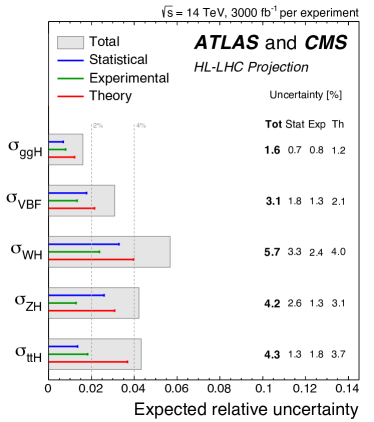
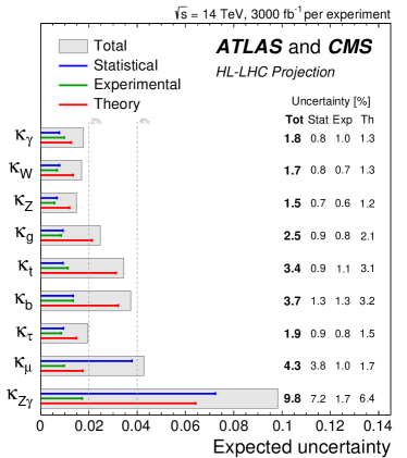
where $h$ represents the field of the physical Higgs boson, which is what remains after the EWSB. The Higgs boson mass is $m_{H}=\sqrt{2}\lambda v\simeq 125$ GeV, $v=\frac{1}{\sqrt{\sqrt{2}G_{F}}}\simeq 246$ GeV is the vacuum expectation value, and $G_{F}$ is the Fermi constant. In the SM, $\lambda_{3}=\lambda_{4}=\lambda=m_{H}^{2}/(2\,v^{2})$ represents the strength of the coupling of the Higgs boson to itself. The couplings of the Higgs boson to the elementary fermions and bosons generate the particle masses. The most recent review of the expected experimental precision on such couplings, including projections for the High-Luminosity LHC (HL-LHC), is presented in the Snowmass Energy Frontier report [6]. Figure 1 summarises the expected precision on the Higgs production cross sections and coupling modifiers $\kappa_{i}$ [7] with 3000 fb^-1 of data that will be collected by ATLAS and CMS at the end of HL-LHC.

In the case of the Higgs self-interaction, the 95% C.L. limits on the coupling modifier $\kappa_{\lambda_{3}}=\frac{\lambda_{3}}{\lambda_{3}^{\mathrm{SM}}}$ (with $\lambda_{3}^{\mathrm{SM}}$ being the expected SM value) are $-0.6<\kappa_{\lambda_{3}}<6.6$ for ATLAS [8] and $-1.24<\kappa_{\lambda_{3}}<6.49$ for CMS [9] with the current LHC data. With HL-LHC data, a 50% precision on the SM value of the self-coupling is expected, which is not sufficient to determine the potential shape.

Figure 1: Projections of the expected precision of the ATLAS and CMS combination on the Higgs production cross sections (left) and $\kappa_{i}$ coupling modifiers (right) including HL-LHC [1] data.

In order to reveal new physics in the Higgs sector, it is necessary to determine the Higgs couplings to elementary fermions and bosons with a percent-level precision and achieve a few percent precision in the measurement of the Higgs self-coupling. This underscores the need for a dedicated Higgs factory.

Linear and circular $e^{+}e^{-}$ machines have been the subject of debate for a long time as well as $\mu^{+}\mu^{-}$ colliders. Recently $\mu^{+}\mu^{-}$ collisions are regaining attention on the international scene, thanks to the impressive physics potential and to new studies on technical feasibility [10].

A Muon Collider (MuC) is a proposed future accelerator in which $\mu^{+}$ and $\mu^{-}$ beams collide at very high center-of-mass energies in a circular machine, thanks to the negligible energy loss of muons due to synchrotron radiation. The current proposal of the International Muon Collider Collaboration (IMCC) [11] aims at 10 TeV center-of-mass energy collisions, with a possible initial phase at 3 TeV [10]. A comprehensive review of the physics potential of MuC experiments at both $\sqrt{s}=3$ and $\sqrt{s}=10$ TeV can be found in Refs. [12, 10, 13].

The determination of the Higgs couplings and self-coupling with an unprecedented accuracy will be feasible with 10 TeV center-of-mass muon collisions. However, the possibility of a $\sqrt{s}=3$ TeV run presents a valuable opportunity for Higgs boson research. Indeed, a MuC can already be viewed as a Higgs factory at $\sqrt{s}=3$ TeV, thanks to the high Higgs boson production cross section and machine luminosity (Sec. 2) and to the detector performance (Sec. 3).

This paper presents the results on the Higgs boson studies obtained at a $\sqrt{s}=3$ TeV MuC with a detailed detector simulation and including the beam-induced background (BIB). The BIB presents a challenge to extracting the physics in a MuC experiment. However, as will be shown in the next sections, the precision achieved is comparable to that claimed by MuC parametric simulation studies that do not take the BIB into account. In these parametric simulations, the detector response is described by functions defined with some assumptions, discussed later in the paper, and applied directly to generator-level quantities.

The experimental facility is introduced in Sec. 2, focusing on the interaction region and the detector shielding. The paper, then, describes the generation of physics and background samples, the detector model and the detector simulation, and the event reconstruction in the presence of the BIB (Sec. 3). The results obtained for the Higgs boson production cross sections times the branching ratio for several decay channels are discussed in detail in Secs. 4.1-4.5, and are compared to other parametric simulation studies in Sec. 4.6. The double Higgs production cross section and the self-coupling precision determination are presented in Secs. 6.1 and 6.2, respectively. The lessons learned on the detector requirements that are necessary for Higgs physics are reported in Sec. 7. Finally, Sec. 8 summarizes the prospects for Higgs physics with a MuC.

2 Experimental environment

A MuC facility consists of several sub-systems, which are described in detail in Refs. [10] and [14]. Here, the main components of a $\sqrt{s}=3$ TeV MuC complex, relevant for evaluating the background effects on the detector, are briefly outlined. The structure includes the elements discussed in Ref. [10] in the exact same sequence: a muon injector, an acceleration ring, and a collision ring. Muons are produced in the decay of pions generated by a high-intensity proton beam impinging on a target with high power (in the order of megawatts). The original muon beam, which has large longitudinal and transverse emittances, is organized in bunches and is directed into a cooling channel. The choice of the technique for cooling the muon beams is dictated by the short lifetime of the muon. The proposed technique is the ionization cooling, currently under investigation [15]. The next step is the beam acceleration. A ring will be dedicated to that operation with a size that can vary depending on the final center-of-mass energy, on the magnet technology available at the time of construction, and on the availability of existing tunnels. Finally, the two muon beams are injected into the collider ring.

2.1 Interaction region and beam-induced background

Figure 2: Left: Arrival times of the main BIB components at the detector relative to the bunch crossing. The light gray band between -1 and 15 ns indicates the assumed readout window for the detector. Right: Energy spectra of the BIB particles that reach the detector within the readout window. The solid and dashed lines refer to the center-of-mass energy of 3 TeV and 1.5 TeV, respectively.

Interaction regions (IR) for a muon collider have been designed by the Muon Accelerator Program (MAP) [16] in the US for different center-of-mass energies: 125 GeV, 1.5 TeV, 3 TeV, and 6 TeV [17]. The studies presented in this paper are based on MAP’s configuration at $\sqrt{s}=1.5$ TeV, since a BIB sample for $\sqrt{s}=3$ TeV was not available at the start of the Higgs analyses. Later in this section, a cross-check for validating this approximation is presented.

This IR was optimized by MAP [18] to maximize the achievable luminosity while minimizing the fluxes of background particles that are produced by the decay of muons in the beams and reach the detector region. In fact, at the center-of-mass energy of 1.5 TeV, the dominant source of background is constituted by electromagnetic showers generated by the interactions of high-energy electrons and positrons with the machine elements. The solution devised by MAP to shield the detector from this irreducible background involves the use of two cone-shaped tungsten absorbers (referred to as “nozzles” throughout the paper), positioned inside the detector along the beam pipe on both sides of the interaction point (IP). The dimensions, shape, and materials of the nozzles have been carefully chosen to maximize the absorption of these particle fluxes while maintaining a high detector acceptance.

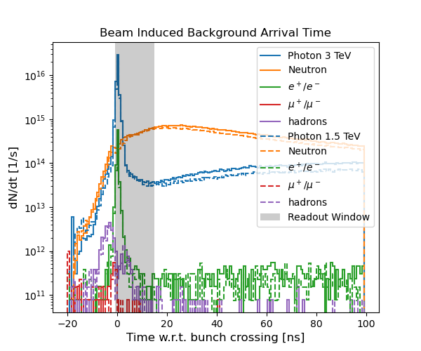
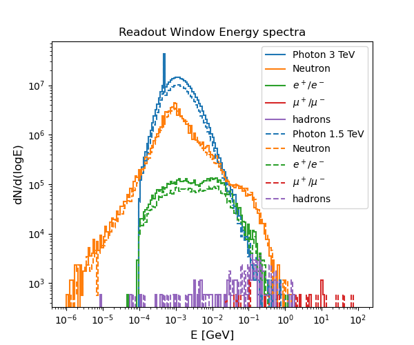
Despite the nozzles, large fluxes of secondary and tertiary particles still reach the detector, but their kinematical properties are such that their effects on the detector can be managed with proper sensor design and advanced event reconstruction methods. Figure 2 shows the main features of particles produced by the in-flight decays of muons and subsequent interactions with the machine, as they enter the detector outer surface. The detector surface is defined as a box containing the detector, which also includes the nozzles and beam pipe boundaries. The distributions are presented for the BIB generated by MAP at $\sqrt{s}=1.5$ TeV with the MARS15 software [19]. In order to cross-check the differences between the $\sqrt{s}=1.5$ TeV and $\sqrt{s}=3$ TeV cases, another BIB sample has been generated at $\sqrt{s}=3$ TeV using the same IR configuration optimized for $\sqrt{s}=1.5$ TeV. This second sample has been generated with FLUKA [20], as described in Ref. [21], and is presented in the same figure. Figure 2 (left) illustrates the arrival time of the background particles at the detector for center-of-mass energies of 1.5 and 3 TeV: a significant fraction of them are outside the assumed detector readout window of [-1, 15] ns (with $t=0$ as bunch-crossing time) and will therefore be rejected. The energy spectra of the particles entering the detector within the readout window are shown in the right panel of Fig. 2. These particles predominantly have momenta below 1 GeV and are expected to primarily affect the detector elements closer to the background entry points.

The differences in the background between the two center-of-mass energies are minimal. The studies described in the remainder of the paper are conducted using signal and physics background samples generated at $\sqrt{s}=3$ TeV. However, as stated before, they utilize the nozzle configuration designed for $\sqrt{s}=1.5$ TeV and the BIB samples generated at the same center-of-mass energy. This is considered a conservative approximation, as preliminary studies indicate the potential to reduce the volume of the nozzles while maintaining the same level of beam-induced background in the detector.

The BIB sample was generated by MAP using a detector solenoidal magnetic field of 3.57 T, which is hence employed also in the current detector model. The BIB particles, given at the detector entry point with their initial kinematical properties and spatial distributions, are propagated into the detector and made interact with each sub-detector by GEANT4 [22]. The detector hits resulting from the BIB particle interactions are stored on disk and then overlaid onto the hits produced by the signals and physics backgrounds to create realistic events. More details about the BIB generation and simulation are reported in Ref. [10].

3 Simulation and reconstruction for signal and background samples

The analysis strategy for measuring the single and double Higgs boson production cross sections is driven by their respective production mechanisms. These mechanisms determine the kinematic properties of the events as well the contributing physics background processes.

In Sec. 3.1, the generation of physics signal and background processes is described. The detector used in the detailed simulation is presented in Sec. 3.2, along with the simulation framework. Section 3.3 explains the digitisation procedure, while Sec. 3.4 discusses the reconstruction algorithms employed.

In this paper, a right-handed reference system is assumed with the origin at the center of the detector, the nominal collision point: the $z$ axis is parallel to the beam direction, the $y$ axis is vertical, and the $x$ axis points to the center of the collider ring.

The MuC software framework [23], based on the ILCSoft [24] framework, has been employed for the detector simulation studies in this paper.

3.1 Signal and background physics processes

3.1.1 Higgs boson production and decay

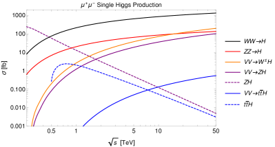
In muon collisions at a center-of-mass energy of 3 TeV with unpolarized beams, the Higgs boson production is dominated by the vector boson fusion (VBF) process, as discussed in Ref. [25]. As shown in Fig. 3, the $\mu^{+}\mu^{-}\to W^{+}W^{-}\nu_{\mu}\bar{\nu}_{\mu}\rightarrow H\nu_{\mu}\bar{\nu}_{\mu}$ process provides the highest contribution, followed by the $\mu^{+}\mu^{-}\rightarrow ZZ\mu^{+}\mu^{-}\rightarrow H\mu^{+}\mu^{-}$ process.

Figure 3: Cross sections for the most important single-Higgs production processes as a function of the center-of-mass energy [25]. The $ZH$ and $t\bar{t}H$ production proceeds via the $s$-channel $\mu^{+}\mu^{-}$ annihilation, while all the other production channels are vector-bosons-fusion processes.

The Higgs decay modes considered in this paper are:

• $H\rightarrow b\bar{b}$,

• $H\rightarrow WW^{*}$,

• $H\rightarrow ZZ^{*}$,

• $H\rightarrow\mu^{+}\mu^{-}$,

• $H\rightarrow\gamma\gamma$.

The sum of their branching ratios is approximately 82%. The $H\rightarrow\tau^{+}\tau^{-}$, $H\rightarrow c\bar{c}$, $H\rightarrow Z\gamma$ modes and the $t\bar{t}H$ production will be the subject of future studies. Each decay mode is affected by different physics backgrounds, which are discussed in the sections dedicated to the corresponding analyses.

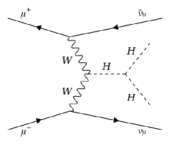
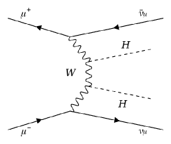
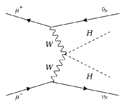
The double-Higgs production at $\sqrt{s}=3$ TeV is illustrated by the Feynman diagrams in Fig. 4, where the dominant tree-level processes are depicted. The diagram on the left is directly related to the $\lambda_{3}$ parameter (see Eq. 1). The two Higgs bosons in the final state are reconstructed in the decay mode $H\rightarrow b\bar{b}$, therefore the major physics background contribution comes from the inclusive process $\mu^{+}\mu^{-}\rightarrow b\bar{b}b\bar{b}$.

Figure 4: Feynman tree-level diagrams representing the major contributions to the double-Higgs production at $\sqrt{s}=3$ TeV. The first diagram on the left represents the process directly related to the Higgs self-coupling.

3.1.2 Event generation

Process	Generator	Kinematical requirements
$\mu^{+}\mu^{-}\to H\nu_{\mu}\bar{\nu}_{\mu};\>H\to b\bar{b}$	WHIZARD	-
$\mu^{+}\mu^{-}\to H\nu_{\mu}\bar{\nu}_{\mu};\>H\to WW^{*}\to q\bar{q}\mu\nu_{\mu}$	WHIZARD	$M(q,\bar{q})>10$ GeV
$\mu^{+}\mu^{-}\to H\nu_{\mu}\bar{\nu}_{\mu};\>H\to\tau^{+}\tau^{-}$	WHIZARD	-
$\mu^{+}\mu^{-}\to H\nu_{\mu}\bar{\nu}_{\mu};\>H\to\mu^{+}\mu^{-}$	MadGraph	-
$\mu^{+}\mu^{-}\to HH\nu_{\mu}\bar{\nu}_{\mu};\>H\to b\bar{b},H\to b\bar{b}$	WHIZARD	-
$\mu^{+}\mu^{-}\to H\mu^{+}\mu^{-};\>H\to WW^{*}\to q\bar{q}\mu\nu_{\mu}$	WHIZARD	$M(q,\bar{q})>10$ GeV
$\mu^{+}\mu^{-}\to H\mu^{+}\mu^{-};\>H\to\mu^{+}\mu^{-}$	MadGraph	$M(\mu,\mu)>100$ GeV
$\mu^{+}\mu^{-}\to H\nu_{\mu}\bar{\nu}_{\mu};\>H\to\gamma\gamma$	MadGraph	$P_{\mathrm{T}}^{\gamma}>10$ GeV, $|\eta^{\gamma}|<2.436$
$\mu^{+}\mu^{-}\to ZZ\nu_{\mu}\bar{\nu}_{\mu};\>Z\to\mu^{+}\mu^{-},Z\to q\bar{q}$	MadGraph	$P_{\mathrm{T}}^{\mu}$ > 1 GeV, $|\eta^{\mu}|$ < 3
		$P_{\mathrm{T}}^{q}$ > 5 GeV, $|\eta^{q}|$ < 3
		$\Delta R(q,\bar{q})$ > 0.2, $\Delta R(q,\mu)>0.05$
$\mu^{+}\mu^{-}\to ZH\nu_{\mu}\bar{\nu}_{\mu};\>Z\to\mu^{+}\mu^{-},H\to b\bar{b}$	MadGraph	$P_{\mathrm{T}}^{\mu}$ > 1 GeV, $|\eta^{\mu}|$ < 3
		$P_{\mathrm{T}}^{q}$ > 5 GeV, $|\eta^{q}|$ < 3
		$\Delta R(q,\bar{q})$ > 0.2, $\Delta R(q,\mu)>0.05$
$\mu^{+}\mu^{-}\to W^{\pm}Z\mu\nu_{\mu};\>W^{\pm}\to q\bar{q},Z\to\mu^{+}\mu^{-}$	MadGraph	$P_{\mathrm{T}}^{\mu}$ > 10 GeV
		$P_{\mathrm{T}}^{q}$ > 5 GeV, $|\eta^{q}|$ < 3
		$\Delta R(q,\bar{q})$ > 0.2, $\Delta R(q,\mu)>0.05$
$\mu^{+}\mu^{-}\to q\bar{q}\nu_{\mu}\bar{\nu}_{\mu}$	WHIZARD	$M(q,\bar{q})>10$ GeV
$\mu^{+}\mu^{-}\to q\bar{q}l\nu$	WHIZARD	$M(q,\bar{q})>10$ GeV
$\mu^{+}\mu^{-}\to Hq\bar{q}\nu\bar{\nu};\>H\to b\bar{b}$	WHIZARD	$M(q,\bar{q})>10$ GeV
$\mu^{+}\mu^{-}\to q\bar{q}q\bar{q}\nu\bar{\nu}$	WHIZARD	$M(q,\bar{q})>10$ GeV
$\mu^{+}\mu^{-}\to HZ;\>H\to WW^{*}\to q\bar{q}\mu\nu_{\mu},Z\to\mu^{+}\mu^{-}$	WHIZARD	$M(q,\bar{q})>10$ GeV
$\mu^{+}\mu^{-}\to\nu_{\mu}\bar{\nu}_{\mu}\mu^{+}\mu^{-}q\bar{q}$	WHIZARD	10 GeV < $M(q,\bar{q})$ < 150 GeV
		$|\eta^{\mu}|$ < 2.5, $|\eta^{q}|$ < 2.5
		$P_{\mathrm{T}}^{\mu}$ > 5 GeV, $P_{\mathrm{T}}^{q}$ > 5 GeV
		$\Delta R(q,\bar{q})$ > 0.3
$\mu^{+}\mu^{-}\to\mu^{+}\mu^{-}\nu_{\mu}\bar{\nu}_{\mu}$	MadGraph	$100<M(\mu,\mu)<150$ GeV,
		$|\eta^{\mu}|<2.66$
$\mu^{+}\mu^{-}\to\mu^{+}\mu^{-}\mu^{+}\mu^{-}$	MadGraph	$100<M(\mu,\mu)<150$ GeV,
		$|\eta^{\mu}|<2.66$
$\mu^{+}\mu^{-}\to t\bar{t};\>t\to Wb,W\to\mu\bar{\nu}_{\mu}$	MadGraph	$M(\mu,\mu)>50$ GeV
$\mu^{+}\mu^{-}\to\gamma\gamma\nu_{\mu}\bar{\nu}_{\mu}$	Madgraph	$P_{\mathrm{T}}^{\gamma}>10$ GeV, $|\eta^{\gamma}|<2.436$
$\mu^{+}\mu^{-}\to ll\gamma$	Madgraph	$P_{\mathrm{T}}^{\gamma}>10$ GeV, $|\eta^{\gamma}|<2.436$
$\mu^{+}\mu^{-}\to ll\gamma\gamma$	Madgraph	$P_{\mathrm{T}}^{\gamma}>10$ GeV, $|\eta^{\gamma}|<2.436$
$\mu^{+}\mu^{-}\to\gamma\gamma$	Madgraph	$P_{\mathrm{T}}^{\gamma}>10$ GeV, $|\eta^{\gamma}|<2.436$

Table 1: Summary of the generated samples indicating the Monte Carlo generator used and the kinematical requirements applied to the final-state particles. $M$ represents the invariant mass of the objects indicated in parentheses. The symbol $q$ stands for $u$, $d$, $s$, $c$, or $b$ quarks, while $l$ stands for electron or muon. If $q\bar{q}$ is present, all possible combination of quark flavours, even different flavours, are considered by WHIZARD/Madgraph. The line in the middle of the table separates the Higgs signal from background processes. If the Higgs boson is not indicated in the process, Yukawa couplings are switched off.

Signal and background samples were produced at leading order with the Monte Carlo event generators MadGraph5_aMC@NLO [26], hereinafter referred to as Madgraph, and WHIZARD [27]. The particle hadronization and showering are performed with PYTHIA version 8.2.0.0 [28].

Recently, WHIZARD authors made available a version with corrections at the next-to-leading order [29] for multi-boson processes, but the VBF processes are not yet ready to be used. An evaluation of the impact of such corrections on the signal to noise ratio for the processes considered in this paper will be the subject of future work.

In this paper, the $Z$-boson and $W$-boson fusion processes are not distinguished experimentally, since such a separation would require the capability to detect the muons of Z-boson fusion that are scattered in the very forward regions of the detector. Moreover, with the requirements of Higgs analyses, the event kinematics is compatible between $Z$-boson and $W$-boson fusion productions [30]. For this reason, in most of the cases, events were generated in the $W$-boson fusion channel, which dominates the production cross sections at this center-of-mass energy. When relevant, the contribution of the $Z$-boson fusion process is evaluated by scaling the process cross section, as explained in Sec. 3.5.

Minimal requirements were applied to the sample generation, in order to speed-up the process without biasing the kinematic properties of the events, whose characteristics at this energy are not yet tested experimentally. Table 1 summarises the requirements applied at generator level for each final state produced.

The generation requirements are applied to $P_{\mathrm{T}}^{i}$, the transverse momentum with respect to the $z$-axis (where $i$ is the particle type), to the invariant mass of two particles $M(i,j)$, to the pseudorapidity $\eta^{i}$ or to the distance between two particles in the $\eta$-$\phi$ space, $\Delta R(i,j)=\sqrt{(\Delta\eta)^{2}+(\Delta\phi)^{2}}$, where $\phi$ is the angle with respect to the $x$-axis in the $x$-$y$ plane.

3.2 Detector simulation

The detector model implemented in the detailed simulation is described in Ref. [10], and here, the main characteristics relevant for the analysis are summarised. The MuC detector is derived from the CLIC Collaboration’s detector concept [31], optimized for $\sqrt{s}=3$ TeV $e^{+}e^{-}$ collisions, and has been modified to incorporate the nozzles.

It consists of a silicon-based tracking system surrounded by electromagnetic and hadronic calorimeters, all immersed in a 3.57 T magnetic field provided by a superconducting solenoid. The magnet iron yoke, designed to contain the return flux of the magnetic field, is instrumented with muon chambers.

Figure 5: The detector model used in the detailed simulation, view in the $y$-$z$ plane. From the innermost to the outermost regions, it includes a tracking system (green), an electromagnetic calorimeter (yellow), a hadronic calorimeter (magenta), a superconducting solenoid (light blue), barrel (light green) and endcap (blue) muon detectors. The nozzles are shown in cyan.

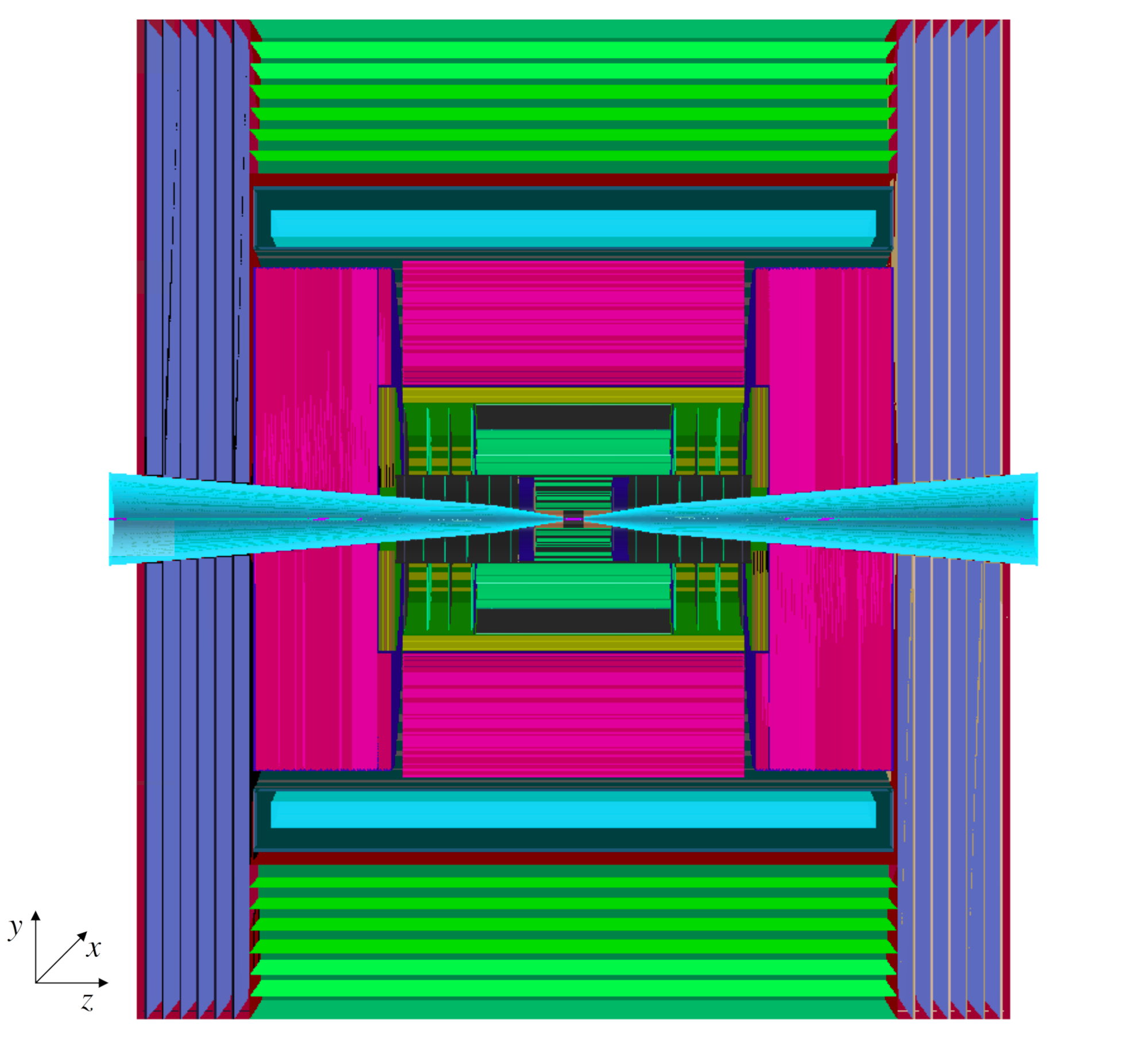
Figure 5 shows the $y$-$z$ view of the detector including the nozzles. From the innermost to the outermost regions with respect to the IP, it features the following components:

• a vertex detector made of double sensor layers of $25\times 25\leavevmode\nobreak\ \mu\mathrm{m}^{2}$ silicon pixels, composed of four central barrel cylinders and four endcap disks on both sides of the barrel;

• an inner tracker with three barrel layers and seven endcap disks on each side made of silicon macropixels with a size of $50\leavevmode\nobreak\ \mu\mathrm{m}\times 1\leavevmode\nobreak\ \mathrm{mm}$;

• an outer tracker composed of three barrel layers and four endcap disks per side of silicon microstrips with a size of $50\leavevmode\nobreak\ \mu\mathrm{m}\times 10\leavevmode\nobreak\ \mathrm{mm}$;

• an electromagnetic calorimeter (ECAL), formed by 40 alternating layers of tungsten absorber and silicon sensors as active material, for a total of 22 radiation lengths, the cell granularity is $5\times 5$ mm²;

• a hadronic calorimeter (HCAL) with 60 alternating layers of steel absorber and scintillating-pad active material, for a total of 7.5 interactions lengths, the cell size is $30\times 30$ mm²;

• a superconductive solenoid generating a magnetic field of $B=3.57$ T;

• an iron return yoke equipped with resistive-plate chambers for muon detection, with seven layers in the barrel and six layers in the endcap, each cell having an area of $30\times 30$ mm².

The simulation of the detector response to particle passage is performed using GEANT4, which is accessed through the MuC software framework [23].

3.3 Digitisation

A MuC event is defined as a generated signal or physics background process with the BIB particles produced in a bunch crossing overlaid. The merging is performed at the level of detector hits, ensuring that both contributions, the signal or the physics background and the BIB, undergo hit digitization in each sensor of the sub-detectors simultaneously. This simulates the process as it would occur during data collection. Marlin [32], one of the packages of the MuC software framework, performs these actions.

A digitisation algorithm is used for the tracker: hit positions and times are smeared with Gaussian distributions representing the spatial and timing resolutions. For ECAL, HCAL, and the Muon System, a digitization is applied where the energies of hits in the same cell are summed up, and the time of the earliest hit is assigned as the time of the digitized hit.

Only hits with arrival times within a specified range relative to the bunch-crossing time ($t=0$) are retained for each sensor to reduce the impact of the BIB component. These time windows are applied on the normalized hit time, defined as $t_{N}=t-D/c$, where $t$ is the absolute time of the hit, $D$ is the distance of the sensor from the interaction point, and $c$ is the speed of light. The time windows are: $[-90,150]$ ps for the vertex detector and $[-180,300]$ ps for the other tracking systems, while for ECAL, HCAL and Muon System hits the range is $\pm 250$ ps. To meet these time requirements, an excellent time resolution is essential. A resolution of 30 (60) ps for the vertex (tracking) system and 100 ps for the calorimeters is assumed in the detailed detector simulation. These time resolutions are expected to be achievable with the technologies developed for HL-LHC, as described in Ref. [10].

3.4 Event reconstruction

The reconstruction algorithms of the physics objects inherited from the ILCSoft package [24] have been adapted for the MuC background conditions, although a complete optimization is still in progress. The Marlin software is employed for the reconstruction of the physics objects. Marlin also makes use of other packages for specific reconstruction tasks, such as the PandoraPFA package [33], which is used for particle flow techniques. A brief description of the utilized algorithms is provided below:

• Tracks: The trajectories of charged particles are reconstructed from the positions of the hits in the silicon tracking stations. Hits are clustered into tracks using two different algorithms. The first one is the Conformal Tracking (CT) [34], the second one makes use of the Combinatorial Kalman Filter, referred to here as the CKF algorithm [35]. The CT algorithm was originally designed for the clean environment of electron-positron collisions and has long running times (order of hours per event with the available computational resources) in the MuC environment due to the presence of the BIB hits. For this reason, it is usually applied to pre-selected hits in regions of interests, e.g. inside calorimetric jet cones or around reconstructed segments of the muon detectors. The CKF algorithm was developed for the proton-proton collision environment and can be executed in the MuC environment in a shorter time (order of minutes per event). The uncertainty on the transverse momentum, $\Delta p_{\mathrm{T}}$, obtained with the CT and CKF algorithms goes from $\Delta p_{\mathrm{T}}/p^{2}_{\mathrm{T}}\approx 1\cdot 10^{-1}$ $(5\cdot 10^{-3})$ GeV^-1 for muons with momentum $p=1$ (100) GeV and polar angle $\theta=13^{\circ}$, to $\Delta p_{\mathrm{T}}/p^{2}_{\mathrm{T}}\approx 5\cdot 10^{-2}$ $(4\cdot 10^{-5})$ GeV^-1 for muons with $p=1$ (100) GeV and $\theta=89^{\circ}$. The track reconstruction efficiency with the CT algorithm is approximately 75% at $\theta=13^{\circ}$ and close to 100% at $\theta=89^{\circ}$. In this paper, the CT algorithm is used for the $H\to WW^{*}$ and $H\to\mu^{+}\mu^{-}$ analyses, whereas the CKF algorithm is employed for the $H\to b\bar{b}$, $H\to ZZ^{*}$, $HH\to b\bar{b}b\bar{b}$, and Higgs width analyses.

• Photons: Photons are defined as clusters of ECAL hits that are not matched to tracks. The PandoraPFA algorithm, which is used for photon reconstruction, takes tracks and calorimeter hits as inputs. Tracks are reconstructed with the CKF algorithm and a track quality filter is applied [10]. An energy threshold of 2 MeV is applied to the calorimeter hits to reduce the BIB contamination. This threshold has a significant impact on the reconstruction of the jets, as will be discussed later. The photon reconstruction efficiency is about 78% for energies below 50 GeV and about 98% for energies above 300 GeV. The photon energy resolution is approximately 13% for energies below 50 GeV and 1.5% for energies above 400 GeV.

• Muons: The PandoraPFA algorithm is also used for muon reconstruction and identification: the tracks reconstructed with either the CT or CKF algorithm are matched to stubs in the muon system. The reconstruction requirements suppress the BIB contamination, at the cost of a low reconstruction and identification efficiency in the forward and backward regions. The efficiency, evaluated in this paper for the CKF tracking algorithm, is about 20$\%$ in the angular regions $10^{\circ}<\theta<20^{\circ}$ and $160^{\circ}<\theta<170^{\circ}$, while it is close to 100$\%$ for $40^{\circ}<\theta<140^{\circ}$. The uncertainty on the muon transverse momentum goes from $\Delta p_{\mathrm{T}}/p^{2}_{\mathrm{T}}\approx 2.1\cdot 10^{-3}$ GeV^-1 for muons with $p_{\mathrm{T}}=2.5$ GeV to $\Delta p_{\mathrm{T}}/p^{2}_{\mathrm{T}}\approx 1\cdot 10^{-4}$ GeV^-1 for muons with $p_{\mathrm{T}}>25$ GeV. The choice of the tracking algorithm employed in a specific Higgs analysis, CT or CKF, depends mainly on the available computing time for each study.

• Jets: Hadronic jets are reconstructed with the following procedure:

  1. tracks are reconstructed as described above and filtered to remove combinatorial background by requiring a minimum number of hits on different tracking layers [10];

  2. calorimeter hits are selected requiring an energy threshold of 2 MeV to remove spurious BIB hits, as in photon reconstruction;

  3. tracks and calorimeter hits are used as inputs to the PandoraPFA algorithm to obtain the reconstructed physics objects;

  4. the $k_{t}$ jet algorithm [36] with a radius parameter of 0.5 is used to cluster the reconstructed physics objects into jets.

  This reconstruction procedure has a jet finding efficiency of $85\%$ for a jet $p_{\mathrm{T}}$ around 20 GeV, and $90\%$ for a jet $p_{\mathrm{T}}$ around 200 GeV. On average, with a $p_{\mathrm{T}}$ threshold of 10 GeV, 13 fake jets are reconstructed per event due to the BIB contribution. Each Higgs analysis involving jets in the final state applies cleaning requirements to minimize the fake rate. More information about fake jets and their mitigation can be found in Ref. [10].

  The jet 4-momentum is calculated by summing the 4-momenta of the clustered physics objects, and the jet direction is defined by the jet momentum direction. A correction is applied to the reconstructed jet energy to take into account detector effects and inefficiencies. This correction is calculated as a function of jet $p_{\mathrm{T}}$ and $\theta$ by comparing reconstructed jets with corresponding truth-level jets (i.e. jets clustered starting from generator-level stable particles). The jet $p_{\mathrm{T}}$ resolution is $35\%$ for a jet $p_{\mathrm{T}}$ around 20 GeV, and above $20\%$ for a jet $p_{\mathrm{T}}$ around 200 GeV.

• $\bm{b}$-tagging: The identification of jets originating from $b$ quarks and their separation from $c$- and light-quark jets is performed by searching for displaced secondary vertices (SV) within the jets [37]. The CT algorithm is used to reconstruct tracks inside the jet cone. A jet is identified as a $b$ jet if a secondary vertex is found with a proper lifetime $\tau=L\,m/P$ greater than 0.2 ps, where $L$ is the distance between the primary and the secondary vertices, $m$ is the mass of the SV, and $P$ is the momentum associated to the SV, calculated as the sum of the momenta of the tracks associated to it. The $b$-jet identification efficiency and misidentification rate have been determined as a function of the jet $p_{\mathrm{T}}$ and $\theta$ with independent samples of $b\bar{b}$, $c\bar{c}$ and light-quark jets [10]. The tagging algorithm has an efficiency of about $45\%$ for a $b$-jet $p_{\mathrm{T}}$ around 20 GeV, and of about $70\%$ for a $b$-jet $p_{\mathrm{T}}$ around 140 GeV with a misidentification rate of about $20\%$ for $c$-jets and from $1\%$ to $5\%$ for light-quark jets. It should be noted that the fake rate in the case of tagged jets is negligible. The algorithm used in the analyses presented in this paper is very simple, a much more advanced algorithm based on artificial-intelligence methods is planned for future updates.

A detailed discussion of the reconstruction performance of these objects can be found in Ref. [10]. Other physics objects, like electrons or $\tau$ leptons, are not treated in this paper due to the lack of personnel. Studies are planned to assess the statistical sensitivity of production cross-section measurements for $H\to e^{+}e^{-}$ and $H\to\tau^{+}\tau^{-}$.

3.5 Analysis path

In multi-TeV muon collisions, Higgs bosons are mainly produced via $W$- or $Z$-boson fusion, i.e. $\mu^{+}\mu^{-}\rightarrow H\nu_{\mu}\bar{\nu}_{\mu}$ or $\mu^{+}\mu^{-}\rightarrow H\mu^{+}\mu^{-}$, respectively. A method to experimentally distinguish the two production modes, which relies on the identification of the forward-scattered muons of the ZZ fusion, is an item for future studies and is not used in this paper. For this reason, in the following analyses, the physics signals are referred to using the compact notation $\mu^{+}\mu^{-}\rightarrow HX$, where $X=\nu_{\mu}\bar{\nu}_{\mu}$ or $\mu^{+}\mu^{-}$.

The kinematic properties of $\mu^{+}\mu^{-}\rightarrow H\nu_{\mu}\bar{\nu}_{\mu}$ and $\mu^{+}\mu^{-}\rightarrow H\mu^{+}\mu^{-}$ are found to be compatible at $\sqrt{s}=3$ TeV. Hence, only the $\mu^{+}\mu^{-}\rightarrow H\nu_{\mu}\bar{\nu}_{\mu}$ process has been generated for the signal samples, the kinematic distributions of which are considered representative of the entire signal. The total signal cross section is then obtained by scaling the $W$-fusion cross section by the $W$-fusion/$Z$-fusion cross-section ratio ($f$):

$$\sigma_{H}=\sigma(\mu^{+}\mu^{-}\rightarrow HX)=\\ \sigma(\mu^{+}\mu^{-}\rightarrow H\nu_{\mu}\bar{\nu}_{\mu})\cdot\left(1+\frac{1}{f}\right).$$ (2)

The factor $\left(1+\frac{1}{f}\right)$ is found to be 1.09 using both WHIZARD and Madgraph. Exceptions to this procedure will be explained in the text.

The integrated luminosity is assumed to be $\mathcal{L}=1$ ab^-1, which is expected to be collected in 5 years of data-taking by a single experiment [10]. It should also be noted that a longer run of 10 years is under discussion, with the goal of collecting $\mathcal{L}=2$ ab^-1. However, the extrapolation of the results to this scenario is beyond the scope of this paper.

The signal and background selection efficiencies ($\epsilon$) are defined as the the ratio between the number of events passing the selection requirements and the corresponding number of generated events. The number $N_{\mathrm{exp}}$ of expected signal and background events is determined with the formula:

$$N_{\mathrm{exp}}=\epsilon\cdot\sigma\cdot\cal{L}\ ,$$ (3)

where $\sigma$ is the production cross section given by the event generator.

The following studies on the Higgs boson cross sections estimate the statistical sensitivity on the production cross section times the branching fraction $\sigma_{H}\times BF(H\to xx)$, where $xx$ denotes any considered final state. The quantity $\sigma_{H}\times BF(H\to xx)$ is indicated with $\sigma(H\to xx)$, and the corresponding uncertainty with $\Delta\sigma(H\to xx)$. It is important to note that in the studies the systematic uncertainties on the luminosity and efficiency are considered negligible: only the statistical sensitivity, resulting from the number of events collected in the data taking, is evaluated.

In several Higgs analyses, machine-learning methods such as Boosted Decision Trees (BDTs) [38] and Multi Layer Perceptrons (MLPs) are employed to enhance the separation between the signal and the physics backgrounds. The BDTs and MLPs have been trained and applied with the TMVA package [39] from the ROOT software suite [40]. Their configuration parameters are set to the default values as defined by TMVA.

4 Determination of Higgs boson cross sections times branching ratios

4.1 $H\to b\bar{b}$ cross section

This section is dedicated to the determination of the statistical sensitivity on the measurement of the $H\rightarrow b\bar{b}$ cross section. Samples of $\mu^{+}\mu^{-}\rightarrow H(\rightarrow b\bar{b})X$ signal events and $\mu^{+}\mu^{-}\to q_{h}\bar{q_{h}}X$, $q_{h}=b,c$ background events have been generated following the prescription of Tab. 1.

Jets are reconstructed as explained in Sec. 3.4 using the CKF algorithm for the input tracks. Jets with $p_{\mathrm{T}}>40$ GeV and $|\eta|<2.5$ are selected to maximize the reconstruction performance and minimize the BIB effects. Both jets from the Higgs decay are required to be identified as $b$-jets, i.e. they have to be associated to a displaced SV. However, applying this requirement directly to the signal and background samples would significantly affect their statistics. Instead, the identification efficiencies and misidentification rates have been determined as a function of jet $p_{\mathrm{T}}$ and $\theta$ (Sec. 3.4) and applied to the signal and background samples as event weights. The light-quark jet misidentification rate has been found negligible, and for this reason light-quark jets have not been included in the background processes. Also the fake jet rate is negligible after the SV requirement.

The expected number of signal and background events is determined with Eq. 3: 59.5k $H\rightarrow b\bar{b}$ events and 65.4k background events are estimated to be collected in 1 ab^-1, as reported in Tab. 2. The di-jet invariant-mass distributions for signal and background are fitted with a double-Gaussian function to obtain models for signal and background.

Process	$\epsilon[\%]$	$\sigma\ [\mathrm{fb}]$	$N_{exp}$
$\mu^{+}\mu^{-}\to H(\to b\bar{b})X$	$19.3$	$308$	$59500$
$\mu^{+}\mu^{-}\to q_{h}\bar{q}_{h}X,\>q_{h}=b,c$	$11.2$	$584$	$65400$

Table 2: Selection efficiency, theoretical cross section, and expected events for the signal and background processes in the $H\to b\bar{b}$ analysis for $\mu^{+}\mu^{-}$ collisions at 3 TeV and $\mathcal{L}=1$ ab^-1.

The signal and background models are used to build a likelihood function and generate samples of pseudo-data according to the expected number of events. An unbinned maximum-likelihood fit is then performed on the invariant-mass distributions of the pseudo-experiments, allowing the signal and background yields to float. In this way, the average $H\rightarrow b\bar{b}$ yield and its uncertainty are extracted. An example of one of the fits is shown in Fig. 6. Due to the limited jet energy resolution, the di-jet invariant mass distribution shows a significant overlap between the Higgs signal and the background, consisting mainly of $Z$ boson decays to $b\bar{b}$ and $c\bar{c}$ pairs. In any case, the number of events is sufficiently high to disentangle the two components on a statistical basis. The $H/Z$ separation will be improved by utilizing a jet reconstruction algorithm that is specifically tuned and optimized for MuC.

The cross section is estimated as follows:

$$\sigma(H\to b\bar{b})=\frac{N_{S}}{\epsilon\cdot\cal{L}}\ ,$$ (4)

where $N_{S}$ is the expected number of signal events and $\epsilon$ is the total signal selection efficiency. Assuming the uncertainties on the efficiency and the luminosity negligible, the statistical uncertainty on the cross section is dominated by the uncertainty on the signal yield. By averaging the results of several pseudo-experiments, the estimated uncertainty on the production cross section is:

$$\frac{\Delta\sigma(H\to b\bar{b})}{\sigma(H\to b\bar{b})}=0.75\%\ .$$ (5)

Figure 6: Example of the di-jet invariant mass fit for one of the pseudo-experiments used to extract the $H\rightarrow b\bar{b}$ yield and uncertainty. Pseudo-data are obtained assuming $\mu^{+}\mu^{-}$ collisions at 3 TeV and $\mathcal{L}=1$ ab^-1 [41].

4.2 $H\rightarrow WW^{*}$ cross section

Figure 7: Distributions of the BDT outputs to separate the $H\to WW^{*}$ signal from the background processes without a Higgs bosons (left) and with a Higgs boson (right). Signal and backgrounds are presented with stacked histograms, normalized to the expected number of events. The black vertical lines indicate the threshold for achieving the optimal signal significance.

The $H\to WW^{*}$ decay is reconstructed in the semileptonic final state, where one $W$ boson decays into a muon and a neutrino and the other one decays hadronically into two jets ($H\to WW^{*}\to qq^{\prime}\mu\nu$) [30]. This final-state has been chosen for its good signal-over-background ratio. In fact, the selection of a high-momentum muon significantly reduces the background from full hadronic final states. On the other hand, the $W$ boson decay to jets has a high branching ratio, hence the semileptonic final state has a higher statistics than the full leptonic final state.

Signal and background samples have been generated as summarized in Tab. 1. Among the physics background processes that could mimic the signal signature, only those with significant cross sections have been considered. They have been grouped into two sets, depending on the presence of the Higgs boson along the process:

1. background processes without a Higgs boson: $\mu^{+}\mu^{-}\to\mu\nu qq^{\prime}$, $\mu^{+}\mu^{-}\to qq^{\prime}l^{+}l^{-}$ and $\mu^{+}\mu^{-}\to qq^{\prime}\nu\bar{\nu}$, with $q=u,d,c,s$ and $l=e,\mu,\tau$;

2. background processes with a Higgs boson: $\mu^{+}\mu^{-}\to H(\to WW^{*}\to qq^{\prime}qq^{\prime})X$, $\mu^{+}\mu^{-}\to H(\to b\bar{b})X$ and $\mu^{+}\mu^{-}\to H(\to\tau^{+}\tau^{-})X$.

In this analysis, jets are first clustered using calorimeter hits, then tracks are reconstructed with the CT algorithm in regions of interest defined by the calorimetric jet cones. Tracks obtained in this way, together with calorimeter clusters, are given as input to the final jet reconstruction. Muons are reconstructed using CT tracks as input. In order to speed-up the muon reconstruction, BIB hits are neglected for this specific task: this approximation does not bias the result since the muon reconstruction requirements suppress the BIB contribution, at the cost of a low efficiency in the forward and backward regions (Sec. 3.4). Signal candidates are formed by combining two reconstructed jets and one muon. The muon is required to have $p_{\mathrm{T}}>10$ GeV and $|\eta|<2.44$ (corresponding to $10^{\circ}<\theta<170^{\circ}$). The two jets must be central with $|\eta|<2.5$ and $p_{\mathrm{T}}>20$ GeV. Requirements are applied to remove fake jets from the analysis: the number of the jet constituents must be greater than two, and the maximum fraction of the jet momentum carried by a single constituent is required to be greater than 0.8. Further details on this prescription can be found in Ref. [30].

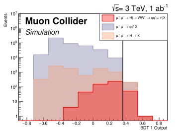
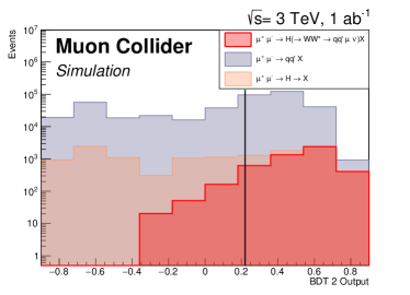
In order to separate signal from backgrounds, two BDTs have been trained: the first to separate the $H\to WW^{*}$ signal from the background processes without a Higgs bosons (listed above in bullet 1), the second to separate the signal from the processes with a Higgs boson (bullet 2). The BDTs have the following observables as inputs:

• the $p_{T}$ and $\theta$ of the selected muon;

• the invariant mass, $p_{T}$, and $\theta$ of the $W\to qq^{\prime}$ candidate formed by two jets;

• the invariant mass, $p_{T}$, and $\theta$ of the Higgs boson candidate;

• the missing transverse momentum, defined as $P^{\mathrm{miss}}_{T}=-\sqrt{P_{x}^{2}+P_{y}^{2}}$ with $P_{x,y}=\sum_{i}p_{x,y}^{\mu_{i}}+\sum_{i}p_{x,y}^{\mathrm{jet}_{i}}$, where the momentum components $p_{x}$ and $p_{y}$ are summed over all reconstructed muons and jets in the event;

• the number of isolated muons in the event, i.e. the muons with $\Delta R=\sqrt{\Delta\phi^{2}+\Delta\eta^{2}}>0.5$ with respect to any jet in the event;

• three acollinearity angles, defined between the momenta $\vec{p}_{i}$ and $\vec{p}_{j}$ of two particles as:

  $$\theta_{\mathrm{acoll}}(i,j)=\pi-\mathrm{acos}\left(\frac{\vec{p}_{i}\cdot\vec{p}_{j}}{p_{i}p_{j}}\right)\ ,$$ (6)

  where $p_{i,j}=|\vec{p}_{i,j}|$ and $i$ and $j$ are: the Higgs boson candidate, the $W\to qq^{\prime}$ candidate, and the selected muon. Hence, the three acollinearity angles are $\theta_{\mathrm{acoll}}(H,\mu)$, $\theta_{\mathrm{acoll}}(H,W\to qq^{\prime})$, and $\theta_{\mathrm{acoll}}(W\to qq^{\prime},\mu)$.

More details on the BDT input variables can be found in Ref. [30]. The output of the BDTs for the signal and backgrounds is shown in Fig. 7. The outputs of the two BDTs are required to be above thresholds determined by maximizing the signal significance

$$\mathcal{S}=\frac{S}{\sqrt{S+B}}\ ,$$ (7)

where $S$ and $B$ are the expected number of signal and background events, respectively, calculated using Eq. 3. Table 3 summarises the efficiencies, theoretical cross sections, and expected number of events passing the selection described. After the event selection, the dominant physics background is the process $\mu^{+}\mu^{-}\to qq^{\prime}\mu\nu$.

Process	$\epsilon[\%]$	$\sigma\ [\mathrm{fb}]$	$N_{exp}$
$\mu^{+}\mu^{-}\to H(\to WW^{*}\to qq^{\prime}\mu\nu)X$	$14.1$	$17.3$	$2430$
$\mu^{+}\mu^{-}\to qq^{\prime}\mu\nu$	$0.05$	5020	2600
$\mu^{+}\mu^{-}\to qq^{\prime}l^{+}l^{-}$	$<0.01$	1040	$<100$
$\mu^{+}\mu^{-}\to qq^{\prime}\nu\bar{\nu}$	$<0.01$	1560	$<100$
$\mu^{+}\mu^{-}\to HX\to WW^{*}X\to qq^{\prime}qq^{\prime}X$	$<0.01$	$108$	$<10$
$\mu^{+}\mu^{-}\to HX\to b\bar{b}X$	$<0.05$	$313$	$<150$
$\mu^{+}\mu^{-}\to HX\to\tau^{+}\tau^{-}X$	$<0.01$	$34.3$	$<4$

Table 3: Selection efficiencies, theoretical cross sections, and expected number of events for signal and background processes in the $H\to WW^{*}$ analysis, with $\mu^{+}\mu^{-}$ collisions at 3 TeV and $\mathcal{L}=1$ ab^-1. The upper limits are determined at $68\%$ Confidence Level.

The statistical sensitivity on the cross section is determined considering this case as a counting experiment. Thus, assuming that the uncertainties on the efficiency and the integrated luminosity are negligible, the error on the $H\to WW^{*}$ cross section is given by:

$$\frac{\Delta\sigma(H\to WW^{*})}{\sigma(H\to WW^{*})}=\frac{\sqrt{S+B}}{S}\ ,$$ (8)

where the formula is derived considering the properties of the Poisson statistics. The statistical sensitivity resulting from the numbers in Tab. 3 is:

$$\frac{\Delta\sigma(H\to WW^{*})}{\sigma(H\to WW^{*})}=2.9\%\ .$$ (9)

4.3 $H\rightarrow ZZ^{*}$ cross section

As with the $H\to WW^{*}$ channel, the $H\to ZZ^{*}$ production has been studied in the semileptonic final state, where one $Z$ boson decays into two muons and the other into two jets, i.e. $\mu^{+}\mu^{-}\to H(\to ZZ^{*})X\to q\bar{q}\mu^{+}\mu^{-}X$. Differently from the $H\to WW^{*}$ analysis, the $Z\to\mu\mu$ decay is fully reconstructed, therefore the background processes in Tab. 3 are considered negligible after applying the selection requirements described below. On the other hand, the $H\to ZZ^{*}$ branching ratio is 10 times lower than $H\to WW^{*}$, and in this measurement the irreducible background $\mu^{+}\mu^{-}\to qq\mu^{+}\mu^{-}X$ becomes the dominant one.

The input tracks of jets and muons have been reconstructed by employing the CKF tracking algorithm. To minimize the number of fake jets, at least one track is required in the jets. Jets must have transverse momentum $p_{\mathrm{T}}>$15 GeV and $|\eta|<1.32$ (corresponding to $30^{\circ}<\theta<150^{\circ}$). Muons are selected with $p_{\mathrm{T}}>10$ GeV. A signal candidate is formed by the combination of two jets and two opposite-charge muons. In order to remove background processes where muons are produced in the jet fragmentation, the distance $\Delta R$ between muons and jets for each combination, which is defined as the distance in the $\eta$-$\phi$ space, must be greater than 0.5. If more than one combination per event is found, the candidate with the invariant mass closer to the Higgs boson mass is selected.

A BDT is used to remove the irreducible background $\mu^{+}\mu^{-}\to qq\mu^{+}\mu^{-}X$. This BDT uses the following inputs: the invariant mass of the Higgs and $Z$ bosons candidates; the angle between the two $Z$ bosons in the laboratory frame; the angles between the muons boosted in the $Z$ boson frame and the flight direction of the $Z$ boson in the laboratory frame; the angles between the $Z$ bosons boosted in the Higgs boson frame and the flight direction of the Higgs boson in the laboratory frame. The simulated signal and background samples are used in the training.

A threshold on the BDT output is determined in order to maximize the signal significance of Eq. 7. The number of expected events after the preselection and the BDT threshold requirement is reported in Tab. 4.

Process	$\epsilon[\%]$	$\sigma\ [\mathrm{fb}]$	$N_{exp}$
$\mu^{+}\mu^{-}\to H(\to ZZ^{*})X\to q\bar{q}\mu^{+}\mu^{-}X$	$15.9$	$0.376$	$60$
$\mu^{+}\mu^{-}\to qq\mu^{+}\mu^{-}X$	$0.69$	$6.18$	$42$

Table 4: Selection efficiency, theoretical cross section, and expected events for signal and background processes in the $H\to ZZ^{*}$ analysis, with $\mu^{+}\mu^{-}$ collisions at 3 TeV and $\mathcal{L}=1$ ab^-1.

As with the $H\to WW^{*}$ analysis, the counting experiment procedure is followed, assuming that the uncertainties on the efficiency and the integrated luminosity are negligible. This yields:

$$\frac{\Delta\sigma(H\to ZZ^{*})}{\sigma(H\to ZZ^{*})}=\frac{\sqrt{S+B}}{S}\ .$$ (10)

Finally, the estimated statistical sensitivity is:

$$\frac{\Delta\sigma(H\to ZZ^{*})}{\sigma(H\to ZZ^{*})}=17\%\ .$$ (11)

4.4 $H\rightarrow\mu^{+}\mu^{-}$ cross section

This section presents the study of the statistical sensitivity on the $H\to\mu^{+}\mu^{-}$ production cross section [42]. The Monte Carlo samples used in the analysis were produced with the MadGraph generator. Two production processes of the Higgs boson are generated: $\mu^{+}\mu^{-}\rightarrow H(\rightarrow\mu^{+}\mu^{-})\nu_{\mu}\bar{\nu}_{\mu}$ and $\mu^{+}\mu^{-}\rightarrow H(\rightarrow\mu^{+}\mu^{-})\mu^{+}\mu^{-}$ featuring two muons and two muonic neutrinos and four muons in the final state, respectively. The main background processes with the same final states as the sought signals are the inclusive channels $\mu^{+}\mu^{-}\rightarrow\mu^{+}\mu^{-}\nu_{\mu}\bar{\nu}_{\mu}$ and $\mu^{+}\mu^{-}\rightarrow\mu^{+}\mu^{-}\mu^{+}\mu^{-}$, from which the contributions from the signal are removed, and $\mu^{+}\mu^{-}\rightarrow t\bar{t}\rightarrow W^{+}W^{-}b\bar{b}$ ($W^{\pm}\rightarrow\mu^{\pm}\nu_{\mu}[\bar{\nu}_{\mu}]$). In order to reduce the computational time of the event simulation and reconstruction, the BIB was not overlaid to the physical processes, since it was shown to have a minimal impact on the muon reconstruction [10]. A cross-check was performed to verify this assumption, as explained later in this section.

The $H\to\mu^{+}\mu^{-}$ analysis proceeds in two steps. First, a loose preselection is applied to identify events with a potential Higgs boson candidate and to suppress part of the low-energy background, then a final event selection is performed using two BDTs. In order to remove a fraction of the physics backgrounds, two opposite-charge muons are required with $p_{\mathrm{T}}>5$ GeV in the angular region $|\eta|<2.44$. Further requirements are applied to the dimuon invariant mass and momenta: $105<m_{\mu\mu}<145$ GeV, $p_{\mathrm{T}}(\mu^{+}\mu^{-})>30$ GeV, and $p_{\mathrm{T}}(\mu^{+})+p_{\mathrm{T}}(\mu^{-})>50$ GeV.

Figure 8: Stack of the $m_{\mu\mu}$ distributions for the selected signal and background events [41]. The distributions have been normalized to the expected number of events with $\mu^{+}\mu^{-}$ collisions at 3 TeV and $\mathcal{L}=1$ ab^-1, reported in Tab.5.

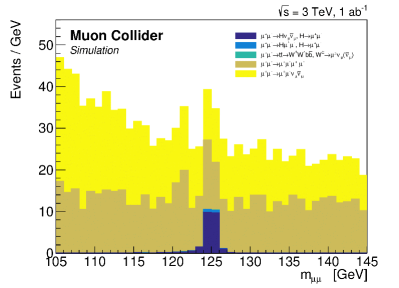
After this preselection, a BDT classifier is trained to discriminate the total signal from the background $\mu^{+}\mu^{-}\rightarrow\mu^{+}\mu^{-}\nu_{\mu}\bar{\nu}_{\mu}$. A second BDT classifier is trained independently for separating the signal from the background $\mu^{+}\mu^{-}\rightarrow\mu^{+}\mu^{-}\mu^{+}\mu^{-}$. The BTDs exploit observables of the two final-state muons (the $p_{\mathrm{T}}$ scalar sum, the angular separation $\Delta R=\sqrt{\Delta\phi^{2}+\Delta\theta^{2}}$, the cosine of the angle between the three-momenta, the cosine of the angle of $\mu^{-}$ momentum in the dimuon rest frame with respect to the dimuon-system direction in the laboratory frame), of the dimuon system (the boost $\beta_{\mu\mu}$, the transverse momentum, the polar angle and the modulus of the three-momentum, the recoil mass), and event observables (the total visible energy, the total visible energy minus the dimuon-system energy, the missing transverse momentum). A cut on the BDT scores is used to select the final samples. The cut values are chosen to maximize the signal significance $\mathcal{S}$, as defined in Eq. 7, and events are required to satisfy at least one of the two BDT requirements.

Process	$\epsilon[\%]$	$\sigma\ [\mathrm{fb}]$	$N_{exp}$
$\mu^{+}\mu^{-}\rightarrow H(\rightarrow\mu^{+}\mu^{-})\nu_{\mu}\bar{\nu}_{\mu}$	$22.12$	0.109	24.2
$\mu^{+}\mu^{-}\rightarrow H(\rightarrow\mu^{+}\mu^{-})\mu^{+}\mu^{-}$	$16.31$	0.010	1.63
$\mu^{+}\mu^{-}\rightarrow\mu^{+}\mu^{-}\nu\bar{\nu}_{\mu}$	$5.74$	11.09	637
$\mu^{+}\mu^{-}\rightarrow\mu^{+}\mu^{-}\mu^{+}\mu^{-}$	$0.160$	297.40	476
$\mu^{+}\mu^{-}\rightarrow t\bar{t}\rightarrow W^{+}W^{-}b\bar{b},$ $W^{\pm}\rightarrow\mu^{\pm}\nu_{\mu}(\bar{\nu}_{\mu})$	$0.34$	0.32	1.1

Table 5: Selection efficiency, theoretical cross section, and expected events for signal and background processes in the $H\to\mu^{+}\mu^{-}$ analysis, with $\mu^{+}\mu^{-}$ collisions at 3 TeV and $\mathcal{L}=1$ ab^-1.

In Fig. 8 is shown the distribution of the dimuon mass $m_{\mu\mu}$ for the expected signal and background events in 1 ab^-1 of data. The corresponding yields are listed in Tab. 5.

The number of signal events $N_{S}$, which is used to calculate the production cross section in Eq .4, can be determined with a fit to the $m_{\mu\mu}$ distribution. The expected uncertainty on $N_{S}$ is estimated with a toy Monte Carlo study. The signal and background models are build from a parameterization of the distributions of Fig. 8. $N_{S}$ is then determined with an unbinned extended maximum-likelihood fit in 10000 pseudo experiments: the $N_{S}$ distribution is centered around 25.8 with an RMS of 9.9. Assuming negligible uncertainties on the selection efficiency and on the integrated luminosity, the relative uncertainty on $N_{S}$ can be considered as the statistical uncertainty of the cross-section measurement:

$$\frac{\Delta\sigma(H\rightarrow\mu^{+}\mu^{-})}{\sigma(H\rightarrow\mu^{+}\mu^{-})}=38\%\ .$$ (12)

It is worth noting that the possibility of identifying the $ZZ$-fusion processes, as outlined in Sec. 3.5, would significantly reduce the $\mu^{+}\mu^{-}\rightarrow\mu^{+}\mu^{-}\mu^{+}\mu^{-}$ background and improve the cross-section sensitivity. To get a rough assessment of the BIB impact to this study, the signal sample $\mu^{+}\mu^{-}\rightarrow H\nu_{\mu}\bar{\nu}_{\mu}$ was reconstructed with the BIB superimposed and compared to the case without BIB at the preselection level of the analysis. The $H\rightarrow\mu^{+}\mu^{-}$ selection efficiency results reduced by about 2%, while the width of the dimuon mass peak degrades only by a few percent which is within the reached precision.

4.5 $H\to\gamma\gamma$ cross section

The experimental signature for the process $\mu\mu\to H(\to\gamma\gamma)X$ consists of two high-$p_{\mathrm{T}}$ photons with an invariant mass compatible with the Higgs boson mass. The signal and physics background processes are generated with MadGraph. The list of the considered backgrounds and their production cross sections is reported in Tab. 6, where only processes with photons in the final state and the highest cross sections are taken into account. The processes with leptons in the final state can pass the event selection because of photon misidentification.

Events are selected with at least two reconstructed photons having $E>15$ GeV, $p_{\mathrm{T}}>10$ GeV, and $|\eta|<2.436$. The most energetic photon must have a $p_{\mathrm{T}}>40$ GeV. If more than two photons in the event fulfill these requirements, the two with the highest energy are selected. The invariant mass of the two photons must satisfy the condition $m_{\gamma\gamma}>40$ GeV.

After the preselection, signal and background events are classified using a BDT. The following variables are used for the classification: the invariant mass $m_{\gamma\gamma}$ and the transverse momentum $p_{\mathrm{T}}(\gamma\gamma)$ of the di-photon system; $p_{\mathrm{T}}$ of the two photons; $\Delta\theta$ and $\Delta\phi$ between the two photons; the acollinearity between the two photons (Eq. 6); the acollinearity between each photon and the Higgs candidate. The BDT is trained by using the signal sample and a mixture of the background samples, merged together with equal weights. The distributions of the BDT output are shown in Fig. 9.

Figure 9: Distribution of the BDT output of the signal and major physics background process. The distributions are stack and normalized to the expected number of events with $\mu^{+}\mu^{-}$ collisions at 3 TeV and $\mathcal{L}=1$ ab^-1 after the preselection cuts. The black vertical line indicates the value of the BDT cut.

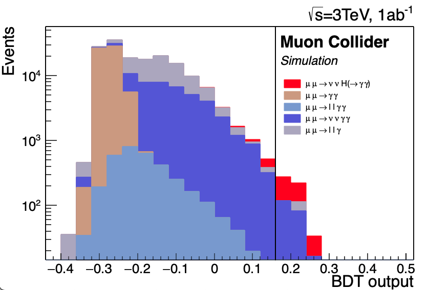
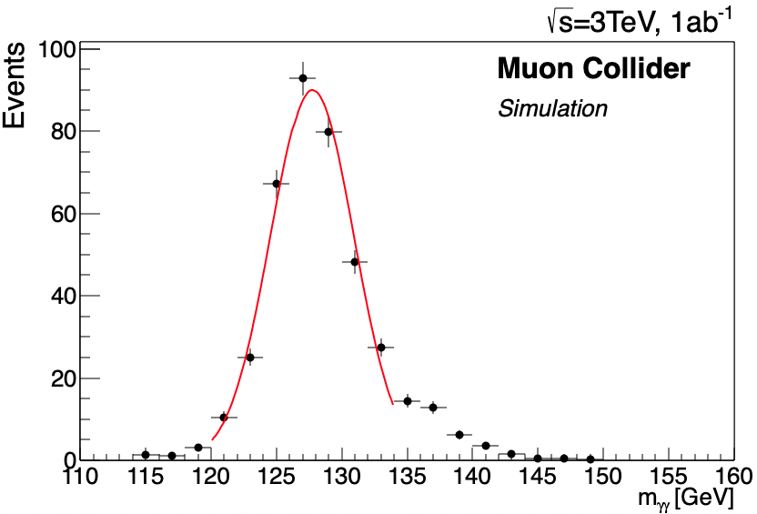
A cut on the BDT output is applied to maximize the significance of Eq.7. The expected number of signal and background events after the BDT requirement are reported in Tab. 6. Fig. 10 shows the invariant mass of the Higgs candidates, with no physics background, after the preselection and the BDT cut. A Gaussian fit of the invariant mass distribution gives a mass resolution of 3.2 GeV for the signal sample.

Figure 10: Distribution of reconstructed $m_{\gamma\gamma}$ for the selected $H\to\gamma\gamma$ events, with no physics background, overlaid with a Gaussian fit. The distribution is normalized to the expected number of events with $\mu^{+}\mu^{-}$ collisions at 3 TeV and $\mathcal{L}=1$ ab^-1.

Process	$\epsilon[\%]$	$\sigma\ [\mathrm{fb}]$	$N_{exp}$
$\mu^{+}\mu^{-}\to H(\to\gamma\gamma)X$	$43.9$	0.91	$396$
$\mu^{+}\mu^{-}\to\nu_{\mu}\bar{\nu}_{\mu}\gamma\gamma$	$1.1$	81.98	$442$
$\mu^{+}\mu^{-}\to l^{+}l^{-}\gamma\gamma$	$0.3$	4.41	$11$
$\mu^{+}\mu^{-}\to l^{+}l^{-}\gamma$	$0.06$	159.01	$31$
$\mu^{+}\mu^{-}\to\gamma\gamma$	$<0.02$	60.15	$<12$

Table 6: Selection efficiencies, theoretical cross sections, and expected events for signal and physics background processes that have a final state with two high energy photons in $\mu^{+}\mu^{-}$ collisions at 3 TeV and $\mathcal{L}=1$ ab^-1.

Assuming that the signal yield is obtained by subtracting the expected number of background events from the observed number of events, after the BDT cut, and assuming a negligible uncertainty on the luminosity and on the signal selection efficiency, the statistical sensitivity on the measurement of the $H\to\gamma\gamma$ cross section can be evaluated as:

$$\frac{\Delta\sigma(H\to\gamma\gamma)}{\sigma(H\to\gamma\gamma)}=\frac{\sqrt{S+B}}{S}\ .$$ (13)

With the expected number of events reported in Tab. 6, the estimated statistical sensitivity is:

$$\frac{\Delta\sigma(H\to\gamma\gamma)}{\sigma(H\to\gamma\gamma)}=7.6\%\ .$$ (14)

4.6 Comparison of results obtained with detailed and parametric simulations

The results presented in the preceding sections are compared with those derived from a parametric description of the detector response and the effects of the BIB, whenever feasible. Given that the BIB represents the primary constraint for physics measurements, it is crucial to demonstrate that suitable detector design and reconstruction algorithms can overcome this limitation.

Furthermore, performing a detailed detector simulation for each physics channel of interest may prove challenging due to the extensive computational times and the consequently significant resources required. This validation provides confidence that the outcomes obtained from parametric simulations remain valid for other physics channels exhibiting similar final states.

To date, the most comprehensive study of Higgs physics at MuC utilizing parametric simulations can be found in Ref. [25]. The detector response has been reproduced by means of the DELPHES [43] program by using parametric functions in the “DELPHES card”. The MuC detector card in DELPHES is a hybrid between CLIC and FCC-hh cards, it is not derived from MuC detector studies. The parametric study considers both the signal and the primary physics background channels, with fiducial requirements adjusted to the detector acceptance to account for the presence of the nozzles.

For the Higgs cross sections, the expected statistical uncertainties have been obtained for $\sqrt{s}=3$ TeV and $\sqrt{s}=10$ TeV collisions, assuming a dataset of 1 and 10 ab^-1, respectively. The former are compared with the results obtained with the detailed simulation and described in this section. The comparison is presented in Tab. 7.

Process	Detailed sim.	Parametric sim.
	$\frac{\Delta\sigma}{\sigma}[\%]$	$\frac{\Delta\sigma}{\sigma}[\%]$
$H\to b\bar{b}$	0.75	0.76
$H\to WW^{*}$	2.9	1.7
$H\to ZZ^{*}$	17	11
$H\to\mu^{+}\mu^{-}$	38	40
$H\to\gamma\gamma$	7.6	6.1

Table 7: Comparison of statistical sensitivities for Higgs boson production cross sections at a $\sqrt{s}=3$ TeV Muon Collider with $\mathcal{L}=1$ ab^-1, obtained with a detailed detector simulation in this paper and a parametric simulation in Ref. [25].

It should be noted that the $H\to b\bar{b}$, $H\to\mu^{+}\mu^{-}$ and $H\to\gamma\gamma$ analyses in Ref. [25] have similar requirements with respect to the detailed simulation studies, and the cross section uncertainties are very close. The $H\to WW^{*}$ and $H\to ZZ^{*}$ analyses in Ref. [25] include additional final states of the considered processes, while this paper focuses only on the final state that contributes most to the sensitivity. Even with these differences, the $H\to WW^{*}$ and $H\to ZZ^{*}$ results are comparable in both frameworks. These comparisons indicate that the proposed detector under realistic conditions, even before full optimization, is already capable of achieving results that are consistent with those of the parametric simulations.

5 Higgs boson width

The Higgs width ($\Gamma_{H}$) is a fundamental parameter of Higgs boson physics, since it is closely connected to the broader picture of the Higgs couplings. The expected value in the SM is $\Gamma_{H}=4.07$ MeV for a 125 GeV Higgs boson [44], a deviation from this value would be a clear indication of new physics in the Higgs sector. Moreover, a model-independent measurement of $\Gamma_{H}$ is an essential input to the Higgs couplings fit, which considers the probability of Higgs boson decays to invisible final states as a free parameter. The proposed method to measure the Higgs width at the HL-LHC is to extract $\Gamma_{H}$ from the interference between the off-shell Higgs boson production and the full amplitude in the $ZZ\to 4l$ channel [1]. The projection for the combined result of the ATLAS and CMS experiments is $\Gamma_{H}=4.1^{+0.7}_{-0.8}$ MeV with about a 17% accuracy [45]. At $e^{+}e^{-}$ colliders, the $e^{+}e^{-}\to HZ$ process with full reconstructed $Z$ bosons allows for the determination of the Higgs boson kinematics independently of the Higgs decay channel [1]. This process provides the primary contribution to the sensitivity on the $\Gamma_{H}$ parameter in global Higgs fits at $e^{+}e^{-}$ colliders. The FCC-ee program, combined with the HL-LHC, expects a $1\%$ precision on the $\Gamma_{H}$ measurement [46], while the expected precision for ILC is at the 2$\%$ level with only the $\sqrt{s}=250$ GeV stage [47]. The projection for the full CLIC program is a sensitivity of 3.5% [48].

At a 3 TeV MuC, the $HZ$ production cross section is relatively small (see Fig.3), therefore the proposed method for the $e^{+}e^{-}$ colliders is not a viable option. Instead, the approach considered for HL-LHC, where $\Gamma_{H}$ is obtained by studying the kinematics of the full $ZZ$ process, is used in this paper [49]. Hence, the pair production of on-shell $Z$ bosons via the VBF process $\mu^{+}\mu^{-}\rightarrow\nu_{\mu}\bar{\nu}_{\mu}ZZ$ is simulated in the detector and reconstructed for the determination of $\Gamma_{H}$. This final state has a contribution coming from the decay of an off-shell Higgs boson, as shown in Fig. 11, therefore the process is sensitive to the couplings of the Higgs boson to $Z$ bosons.

Figure 11: Feynman diagram for on-shell $ZZ$ production via VBF, occurring with an off-shell Higgs propagator.

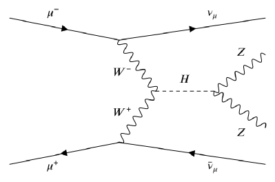
Thanks to the contribution of this process, the production of a pair of $Z$ bosons can be used directly to extract the modifier $\kappa$ of the couplings between Higgs boson and vector bosons, assuming it to be the same for both $Z$ and $W^{\pm}$:

$$\kappa=\frac{g_{HZZ}}{g_{HZZ}^{SM}}=\frac{g_{HWW}}{g_{HWW}^{SM}}\ .$$ (15)

To obtain $\Gamma_{H}$, the measurement of the $H\rightarrow ZZ^{*}$ cross section is also needed (Sec. 4.3). Indeed, the following equation holds [50]:

$$\frac{\sigma(H\rightarrow ZZ^{*})}{\sigma^{SM}(H\rightarrow ZZ^{*})}\propto\frac{\kappa^{4}}{\Gamma_{H}/\Gamma_{H}^{SM}}\ ,$$ (16)

where $\sigma^{SM}(H\rightarrow ZZ^{*})$ and $\Gamma_{H}^{SM}$ are the expected SM values for the $W^{+}W^{-}\rightarrow H\rightarrow ZZ^{*}$ cross section and Higgs boson width, respectively. With $\kappa$ obtained from the $ZZ$ production and the measurement of the $H\rightarrow ZZ^{*}$ cross section (Sec. 4.3), the determination of $\Gamma_{H}$ is finally possible.

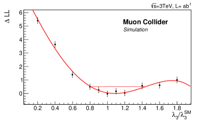
The approach considered for measuring $\kappa$ is to compare the data with different simulation samples generated by varying $\kappa$, and subsequently find the best $\kappa$ value with a likelihood scan. The $\mu^{+}\mu^{-}q\bar{q}$ final state, where $q$ is any quark, has been chosen as a compromise between event counts and precision in the reconstruction of the final state. The relevant processes come from VBF di-boson production with the $\mu^{+}\mu^{-}qq^{\prime}$ final state, namely: $\mu^{+}\mu^{-}\rightarrow\nu_{\mu}\bar{\nu}_{\mu}Z(\rightarrow\mu^{+}\mu^{-})Z(\rightarrow q\bar{q})$, $\mu^{+}\mu^{-}\rightarrow\nu_{\mu}\bar{\nu}_{\mu}H(\rightarrow b\bar{b})Z(\rightarrow\mu^{+}\mu^{-})$, and $\mu^{+}\mu^{-}\rightarrow\nu_{\mu}\mu^{\pm}W^{\pm}(\rightarrow qq^{\prime})Z(\rightarrow\mu^{+}\mu^{-})$. The first two are $WW$-fusion processes and are the ones with the largest dependence on $\kappa$. The latter is a $WZ$-boson fusion process, where the first muon is usually undetected, since it is emitted at very small polar angles. In Ref. [51], it has been verified that the $ZZ$-fusion contribution to the $\Gamma_{H}$ sensitivity is negligible, therefore it is not considered in this analysis.

Several high-statistics simulation samples corresponding to different $\kappa$ values should be produced for determining the uncertainty on $\kappa$. The task of performing the detailed simulation for all these samples is excessively computing intensive and time demanding with the resources available for this study. For this reason a hybrid fast-simulation/full-simulation approach has been used:

• A sample of $\mu^{+}\mu^{-}qq^{\prime}$ events has been generated with Madgraph with $k=1.0$ and processed with the detailed detector simulation. This sample has been used to determine the reconstruction efficiencies and momentum resolutions for jets and muons, as well as their dependence on the kinematics.

• $\mu^{+}\mu^{-}qq^{\prime}$ samples have been generated with Madgraph, corresponding to 17 values of $\kappa$ ranging form $-0.2$ to $2.0$, to which the resolutions and efficiencies obtained with the detailed simulation have been applied. Resolutions are applied as smearing factors and efficiencies as event weights. The dependence on the kinematics is taken into account.

• These fast-simulation samples are then used to perform the likelihood scan for the determination of the uncertainty on $\kappa$.

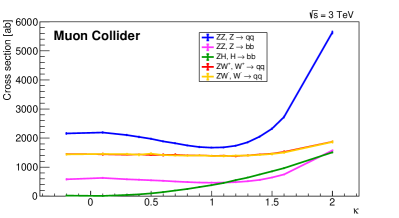
The cross sections, calculated with Madgraph, of the main processes that contribute to $\mu^{+}\mu^{-}qq^{\prime}$ are shown in Fig. 13 as a function of $\kappa$. It is evident that $\mu^{+}\mu^{-}\rightarrow\nu_{\mu}\bar{\nu}_{\mu}Z(\rightarrow\mu^{+}\mu^{-})Z(\rightarrow q\bar{q})$ is the most sensitive process to $\kappa$.

Figure 12: Cross sections obtained with Madgraph for the processes considered in the determination of the Higgs coupling modifier $\kappa$.

In this analysis, jets and muons are reconstructed as in Sec. 4.3. Events are selected requiring at least two opposite-charge muons with $p_{\mathrm{T}}>15$ GeV and at least two jets with $p_{\mathrm{T}}>20$ GeV. The positive and negative muons with the highest $p_{\mathrm{T}}$ are selected and required to have an invariant mass between 85 and 97 GeV. Jets with a $\Delta R<0.5$ with respect to any of the two selected muons are discarded. To remove fake jets from the BIB, jets are required to contain at least one track. After this requirement fake jets are assumed to be negligible and they are not considered in the analysis. Finally, the two jets with the highest $p_{\mathrm{T}}$ are selected and required to have an invariant mass greater than 50 GeV. The invariant mass $M_{\mu\mu qq}$ of all selected final state objects ($\mu^{+}$, $\mu^{-}$ and the two jets) is required to be between 180 and 1800 GeV.

Likelihood values are calculated comparing 2-dimensional distributions of $M_{\mu\mu qq}$ and $\theta_{ZZ}$ (i.e. the angle between the reconstructed $Z$ bosons in the laboratory frame) between data and simulation. Pseudo-datasets are generated from the distribution with $\kappa=1$. For each pseudo-dataset, the likelihood difference $-2\Delta\log(L)$ as a function of $\kappa$ is obtained. These values are fitted to a 6^th degree polynomial, and the $1\,\sigma$ interval is estimated as the interval around $\kappa=1$ where the fitted polynomial has a value below 1. For each pseudo-dataset, upper and lower bounds are found, and the final result is given by the average of 50 pseudo-datasets. The obtained likelihood scans are shown in Fig. 13. The final result on the $\kappa$ uncertainty interval is $\kappa=1^{+17\%}_{-12\%}$.

Figure 13: Likelihood for th determination of $\kappa$, fitted with a 6^th degree polynomial. Likelihood scans for 50 pseudo-experiments are overlaid (red lines), the points represent the average and standard deviations of $-2\Delta\log(L)$ for the considered $\kappa$ values.

Starting from Eq. 16, it can be written as:

$$\Delta\Gamma_{H}=\Delta\sigma(H\rightarrow ZZ^{*})\oplus(4\,\Delta\kappa)\ ,$$ (17)

where the $\oplus$ symbol means squared sum. Taking $\Delta\sigma(H\rightarrow ZZ^{*})$ from Sec. 4.3, the final result is found to be

$$\frac{\Gamma_{H}}{\Gamma_{H}^{SM}}=1^{+71\%}_{-88\%}\ .$$ (18)

As was done for the Higgs boson cross sections in Sec. 4.6, the result on the Higgs width is compared with that obtained with a parametric simulation. In particular, it has been compared with the study presented in Ref. [51], where the detector effects are taken into account with a fast simulation based on DELPHES, which uses the MuC detector card discussed in Sec. 4.6. In the article cited above, the precision on the Higgs width, obtained with a fully general $\kappa$-fit, is 24$\%$. However, the contribution obtained by exploiting only the $\mu^{+}\mu^{-}\rightarrow\nu_{\mu}\bar{\nu}_{\mu}ZZ$ and $\mu^{+}\mu^{-}\rightarrow\nu_{\mu}\bar{\nu}_{\mu}W^{+}W^{-}$ channels is 58$\%$ [52]. The latter result includes different final states ($4q$, $2q2l$, and $l\nu qq$) and is of the same order as the one presented in this section ($\Delta\Gamma_{H}\sim 80\%$), which uses only $2q2\mu$ events and is based on the detailed detector simulation. Furthermore, the aforementioned paper [51] obtained an uncertainty of $\Delta\Gamma_{H}=3.4\%$ for the case of $\sqrt{s}=10$ TeV muon collisions: future simulation studies with the $\sqrt{s}=10$ TeV detector will be necessary to confirm these statements. We notice also that the study presented in Ref. [50] shows how the introduction of a system for tagging forward muons up to $|\eta|<6$ could enable a Higgs width precision up to $1^{+2.1\%}_{-0.4\%}$ at a $\sqrt{s}=10$ TeV muon collider, which is competitive with the expectation from FCC-ee combined with HL-LHC [46]. Again, these results should be validated with the detector simulation that includes a forward muon tagging system.

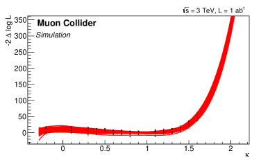
6 Trilinear coupling

In this section, the measurement of the trilinear coupling at a $\sqrt{s}=3$ TeV MuC is studied with the detailed detector simulation. The state-of-the-art projections on the $\kappa_{\lambda_{3}}$ sensitivity obtained with MuC parametric simulations are reported in Refs. [13, 10]. In those studies, the 68$\%$ confidence-level bound, obtained with $\mathcal{L}=1$ ab^-1 of data collected at $\sqrt{s}=3$ TeV, is composed of two intervals, corresponding to two different likelihood minima: $0.73<\kappa_{\lambda_{3}}<1.35$ and $1.85<\kappa_{\lambda_{3}}<1.94$. It is also stated that the second minimum can be removed by collecting $\mathcal{L}=2$ ab^-1, leading to a 68$\%$ confidence level of $0.85<\kappa_{\lambda_{3}}<1.16$. In the following, the case with $\mathcal{L}=1$ ab^-1 is considered for the detailed simulation, but just the first minimum, closer to the SM value, is studied and compared with the parametric simulation.

Sec. 6.1 describes the measurement of the double Higgs production ($HH$), which is the first step towards a measurement of the trilinear coupling. Then, the trilinear coupling extraction is presented in Sec. 6.2.

6.1 $HH\rightarrow b\bar{b}b\bar{b}$ cross section determination

The $HH$ production is studied using the $H\to b\bar{b}$ decay for both Higgs bosons, since this final state exhibits the highest branching ratio, and the channel with four $b$ quarks provides the highest statistics [53, 54]. The contribution of other final states, like $HH\to b\bar{b}\gamma\gamma$, will be investigated in future studies.

In this analysis, at least four reconstructed jets are required in the event with a minimum $p_{\mathrm{T}}$ of 20 GeV. Input tracks for jets are obtained with the CKF algorithm. The $b$-jet identification efficiencies and the misidentification rates presented in Sec. 3.4, have been applied to the reconstructed jets as a function of the jet $p_{\mathrm{T}}$ and taking into account the flavour composition of the final state, as with the $H\to b\bar{b}$ analysis in Sec. 4.1. This procedure replaces the direct application of the tagging algorithms to the simulated samples with the BIB overlaid, which requires computing resources not currently available.

To reconstruct the $HH$ events, all possible two-jet combinations are formed, in which at least one jet is requested to be identified as a $b$-jet. Two Higgs boson candidates are then built from the two jet pairs whose invariant masses $m_{12}$ and $m_{34}$ minimize the figure of merit:

$$F=\sqrt{(m_{12}-m_{H})^{2}+(m_{34}-m_{H})^{2}}\ ,$$ (19)

where $m_{H}$ is the nominal Higgs boson mass.

The main physics background contribution comes from processes with four heavy-quark jets in the final state, $\mu^{+}\mu^{-}\to q_{h}\bar{q}_{h}q_{h}\bar{q}_{h}X$ ($q_{h}=b$ or $c$), which comprise multiple intermediate electroweak gauge bosons. The other important source of background is the process $\mu^{+}\mu^{-}\to Hq_{h}\bar{q}_{h}X\to b\bar{b}q_{h}\bar{q}_{h}X$ where the $HHH$ vertex is not present. Physics backgrounds resulting from light quarks and fake jets are assumed negligible. The rationale for this assumption is that advanced tagging methods, based on machine learning techniques, should be capable of rejecting these events while keeping the signal, as discussed later in Sec. 6.2. A summary table presenting the signal and background processes, along with their cross sections and expected event yields, is provided in Tab. 8.

Process	$\epsilon[\%]$	$\sigma\ [\mathrm{fb}]$	$N_{exp}$
$\mu^{+}\mu^{-}\to HHX\to b\bar{b}b\bar{b}X$	$27.5$	0.31	$84$
$\mu^{+}\mu^{-}\to H(\to b\bar{b})q_{h}\bar{q}_{h}X$	$24.72$	3.1	$761$
$\mu^{+}\mu^{-}\to q_{h}\bar{q}_{h}q_{h}\bar{q}_{h}X$	$18.1$	5.9	$1066$

Table 8: Selection efficiencies, theoretical cross sections, and expected events for signal and background processes in the $HH\rightarrow b\bar{b}b\bar{b}$ analysis, with $\mu^{+}\mu^{-}$ collisions at 3 TeV and $\mathcal{L}=1$ ab^-1.

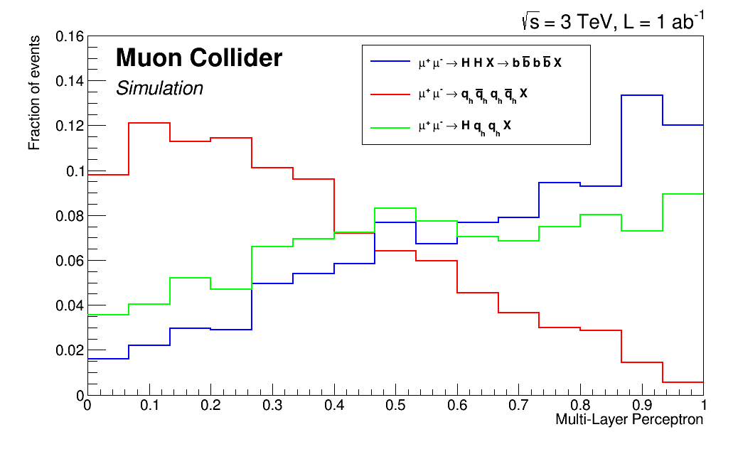
A Multilayer Perceptron (MLP) [39] has been trained on twelve observables to separate the signal events from the physics background $\mu^{+}\mu^{-}\to q_{h}\bar{q}_{h}q_{h}\bar{q}_{h}X$:

• the invariant masses of the jet pairs with the highest (leading candidate) and the lowest (sub-leading candidate) transverse momentum;

• the module of the vectorial sum of the four jet momenta;

• the sum of the four jet energies;

• the angle between the two jets relative to the leading candidate;

• the maximum separation angle between the jets in the event;

• the angle between the highest-$p_{\mathrm{T}}$ jet in the pair relative to the leading candidate, and the angle between the highest-$p_{\mathrm{T}}$ jet in the pair relative to the sub-leading candidate, with respect to the $z$-axis;

• the four jet transverse momenta.

The MLP output distributions for the $HH$ signal and background samples are shown in Fig. 14. It can be observed that a good separation between the $HH$ and $q_{h}\bar{q}_{h}q_{h}\bar{q}_{h}X$ processes is achieved. It has been verified that an additional MLP to separate the signal from the $\mu^{+}\mu^{-}\to H(\to b\bar{b})q_{h}\bar{q}_{h}X$ background does not improve significally the measurement, since the kinematic properties of this process are very similar to those of the signal.

Using the MLP output distributions, pseudo-datasets have been generated according to the expected number of events. The yield of the $HH$ signal is extracted by fitting the MLP distribution: an average statistical uncertainty of approximately 33% is obtained on the signal yield. The $HH$ cross section is calculated with Eq. 4. Therefore, assuming negligible uncertainties on the selection efficiency and integrated luminosity, the statistical uncertainty on the double-Higgs production cross section is:

$$\frac{\Delta\sigma(HH\rightarrow b\bar{b}b\bar{b})}{\sigma(HH\rightarrow b\bar{b}b\bar{b})}=33\%\ .$$ (20)

Figure 14: Distributions of the MLP output for the $HH$ signal and the main background contributions. The distributions are normalized to unit area.

At this time, there is no estimate of the statistical sensitivity on the $HH$ cross section based on a parametric simulation of the detector. Reference [55] reports only the expected uncertainty on the trilinear coupling without considering detector effects, as explained in the next section.

6.2 Trilinear Higgs coupling precision determination

The evaluation of the uncertainty on the trilinear Higgs boson self-coupling has been conducted using the simulated sample $\mu^{+}\mu^{-}\to HHX\to b\bar{b}b\bar{b}X$, described in Sec. 6.1. The total double-Higgs production cross section is sensitive to the value of the trilinear self-coupling: Fig. 4 shows the three Feynman diagrams that primarily contribute to the double-Higgs production. The one on the left, where two Higgs bosons are produced via an off-shell Higgs ($H^{*}$), is the only process directly influenced by the value of the trilinear Higgs self-coupling. The different kinematics of the $HH$ events coming from $H^{*}$ is exploited to extract the value of $\lambda_{3}$. The strategy employed to estimate the uncertainty on the trilinear Higgs self-coupling is as follows:

• Samples of double-Higgs events are generated with WHIZARD for different values of $\kappa_{\lambda_{3}}=\lambda_{3}/\lambda_{3}^{SM}$: 0.2, 0.4, 0.6, 0.8, 0.9, 1.0, 1.1, 1.2, 1.4, 1.6, 1.8. Subsequently, the samples are simulated and reconstructed with the procedure described in Sec. 6.1. The $\kappa_{\lambda_{3}}=1$ case represents the SM signal. Tab. 9 shows the expected number of $HH$ events for different $\kappa_{\lambda_{3}}$ hypotheses;

  $\kappa_{\lambda_{3}}$	$\sigma$ [fb]	$\epsilon$ [%]	Nevents
  0.2	0.52	30.1	169
  0.4	0.48	29.3	141
  0.6	0.41	28.1	116
  0.8	0.35	27.5	97
  0.9	0.33	27.6	92
  1.0	0.31	27.2	84
  1.1	0.29	25.7	74
  1.2	0.27	25.7	71
  1.4	0.25	26.5	68
  1.6	0.24	25.1	61
  1.8	0.25	24.8	61

  Table 9: Theoretical cross section values, selection efficiencies, and expected number of $HH\to b\bar{b}b\bar{b}$ events for all $\kappa_{\lambda_{3}}$ hypotheses, assuming 1 ab^-1 of integrated luminosity at $\sqrt{s}=3$ TeV.

• Two MLPs are trained independently:

  1. The first MLP is the same as the one used for the $HH$ cross section determination in Sec. 6.1 to separate the SM signal ($\kappa_{\lambda_{3}}=1$) from the physics background.

  2. The other MLP is trained on four variables to differentiate between the $\mu^{+}\mu^{-}\to HH\nu_{\mu}\bar{\nu}_{\mu}\to b\bar{b}b\bar{b}\nu_{\mu}\bar{\nu}_{\mu}$ process, where the Higgs pair is produced exclusively via an off-shell $H^{*}$ (left diagram in Fig. 4), and the other two contributions. The rationale behind this approach is to construct a MLP that leverages the kinematic properties specific to the production of Higgs pairs via an off-shell Higgs boson, which is indicative of the trilinear Higgs self-coupling. This allows for the separation of this process from other double-Higgs production processes. The variables that allow the best separation are: the angle between the two Higgs boson momenta in the laboratory frame, the angle between the highest-$p_{T}$ jet momenta of each pair with respect to the $z$ axis, and the helicity angle of the two Higgs boson candidates.

• The scores of the two MLPs for the considered samples have been arranged in 2-dimensional histograms. To obtain the expected data distribution, 2-dimensional templates of the signal and background components are built for each $\kappa_{\lambda_{3}}$ hypothesis. Signal and background yields calculated in Tabs. 8 and 9 are used to weight the templates.

• Pseudo-datasets are generated with the total 2D template for the $\kappa_{\lambda_{3}}=1$ hypothesis. For each pseudo-experiment, the likelihood difference $-\Delta\mathrm{log}(L)$ is calculated as a function of $\kappa_{\lambda_{3}}$ by comparing the pseudo-data distribution to the $\kappa_{\lambda_{3}}$ templates.

• The log-likelihood profile has been fitted with a polynomial function of fourth degree. The uncertainty on $\kappa_{\lambda_{3}}$ at 68% C.L. is estimated as the interval around $\kappa_{\lambda_{3}}=1$ where the fitted polynomial has a value below 0.5.

As shown in Tab. 9, the expected production cross sections for $\kappa_{\lambda_{3}}>1$ are very similar. Distinguishing between them requires a signal-to-noise separation better than what is currently achievable. Therefore, the result achievable with the detailed detector simulation, including the BIB overlay, and the current version of the reconstruction algorithms, is significantly biased due to the non-optimized algorithms. This result does not provide an adequate representation of the true potential of MuC for this measurement. Although many improvements are currently in progress, they are not yet ready to be applied to the analysis. Nevertheless, it is possible to assess the impact of the new algorithms on the measurement, as discussed in the following:

• With a dedicated machine-learning algorithm that exploits the jet sub-structure, it is possible to identify $b$-jets with a performance comparable to that of hadron colliders. Machine-learning algorithms that exploit information about the jet sub-structure are currently employed at LHC to enhance the performance of jet flavor identification both in the central region of $pp$ collisions, like the DeepJet algorithm [56] at CMS, and in the forward region at LHCb [57]. At a MuC, $b$-jets from $HH$ are expected to be produced predominantly in the forward region, and an excellent vertex detector is considered for the MuC detector, as the one of LHCb that is optimized for having the best vertex reconstruction performance. For these reasons, the LHCb tagging capabilities are assumed for the MuC expectation: the $b$-tagging efficiency and $c$-mistag are taken from Ref. [57], while light jet mistag is assumed negligible, as expected from LHCb data. A working point for the $HH$ analysis has been determined by maximizing the significance ($S/\sqrt{S+B}$) of $HH$ events across various configurations of LHCb $b$-tagging and $c$-mistag performance. The optimal configuration, yielding the highest significance, requires: 3 tagged jet, a total $b$-tagging efficiency of 76$\%$ and a $c$-mistag rate of 20$\%$. Simulated events for $HH$ signal and background processes are re-weighted according to these efficiencies.

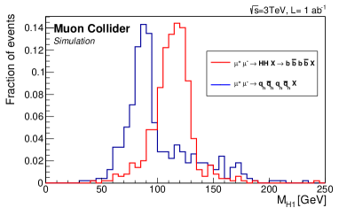
• Several developments are currently underway to minimize the impact of the BIB on both jet reconstruction efficiency and jet energy resolution, aiming to reduce it to a negligible level. For example, the number of BIB hits in the tracker system could be reduced by applying a cutting-edge clustering algorithm capable of identifying and rejecting hits associated with low-momentum BIB particles, which tend to deposit more ionization energy. This strategy aims to decrease the occurrence of spurious tracks, thereby enhancing the overall tracking performance. The impact of such an algorithm is evaluated by studying the jet reconstruction performance without overlaying the BIB in the analysis, and reducing the calorimeter energy thresholds from 2 MeV to 200 KeV. The last assumption leads to an improvement in the jet energy resolution, as already demonstrated in Ref. [10]. The impact of the jet energy resolution improvements on the $HH$ analysis can be understood by comparing the invariant mass distribution of the leading Higgs candidate in $HH$ events to that of $q_{h}\bar{q}_{h}q_{h}\bar{q}_{h}$ events, both without the BIB overlay, Fig. 15 (left). The improved separation between the Higgs and $Z$ boson resonances with respect to what has been obtained in Fig. 6 is evident. The jet momentum resolution in the case without the BIB overlay is in the order of 10%, while the resolution with the BIB is of about 15%. This 10% resolution is used in the analysis to evaluate the trilinear coupling precision.

Figure 15: Left: Invariant mass of the leading Higgs candidate compared between $HH$ events and $q_{h}\bar{q}_{h}q_{h}\bar{q}_{h}$ events, with samples reconstructed without the BIB. Right: $\Delta LL$ as a function of $\kappa$ hypothesis for samples reconstructed without the BIB, selected by assuming LHCb tagging performance ($b$-tagging efficiency of 76$\%$ and $c$-mistag rate of 20$\%$), by requiring three tagged jets in the event.

The likelihood scan obtained with the previous assumptions on the tagging efficiencies and jet momentum resolution is shown in Fig. 15 (right). The uncertainty on the trilinear Higgs self-coupling is found to be $0.81<\kappa_{\lambda_{3}}<1.44$ at 68 $\%$ confidence level. It could be noticed that the upper bound is higher since the number of signal events as a function of $\kappa_{\lambda_{3}}$ varies slowly for $\kappa_{\lambda_{3}}>1.0$, as can be seen in Tab. 9.

The result obtained with the detailed detector simulation can be compared with the first minimum determined with the parametric simulation at the same luminosity of $\mathcal{L}=1$ ab^-1 [13, 10], $0.73<\kappa_{\lambda_{3}}<1.35$. The two results are of the same order.

7 Lesson learned: requirements for Higgs measurements

The Higgs studies presented in this paper allow to establish the detector requirements needed to improve Higgs knowledge. Sec. 4.6 demonstrates that the results obtained for a $\sqrt{s}=3$ TeV MuC with the detailed detector simulation are compatible with the ones determined with the MuC DELPHES card in Ref. [25]. In the same article, it is shown that including those results from parametric simulations in the Higgs couplings fit, together with HL-LHC measurements, improves the overall precision with respect to the HL-LHC-only case.

In general, Sec. 4 has shown how the detector and reconstruction algorithms, discussed in Sec. 3, are sufficient to achieve the precision on single Higgs cross sections obtained with parametric simulations. This has been demonstrated for final states with jets, photons, and muons.

On the other hand, Sec. 6.2 has shown how several improvements on jet reconstruction and identification are needed to improve the precision on the Higgs trilinear coupling with respect to HL-LHC. In fact, the projection for HL-LHC is a precision of about 50% on $\kappa_{\lambda_{3}}$ [1], while $0.81<\kappa_{\lambda_{3}}<1.44$ is expected with the $\sqrt{s}=3$ TeV MuC detector and $\mathcal{L}=1$ ab^-1.

With the previous considerations, the requirements, reported in Tab. 10, are determined in the following way:

• For muons, photons, jets, and $b$-jets the resolution requirements are taken from the performance of the reconstruction described in Sec. 3, and evaluated for objects with $p_{\mathrm{T}}=100$ GeV. The value of $p_{\mathrm{T}}=100$ GeV is chosen because it is the peak of Higgs daughters $p_{\mathrm{T}}$ distribution in 2-body Higgs decays (Fig. 16). For $b$-jets the identification efficiencies and the $c$-mistag rate are also quoted. The motivation for determining the requirements in this way is that these performance is sufficient to achieve results on the cross-section statistical sensitivity comparable with those obtained with the parametric simulations.

• For the measurement of $\lambda_{3}$, the performance of Sec. 3 is not enough to achieve a result that surpasses HL-LHC and of the same order of the parametric simulation. Hence, just for this measurement, the requirements on $b$-jets $p_{\mathrm{T}}$ resolution and identification are taken from the performance described in Sec. 6.2, obtained with reasonable assumptions and that allows a competitive precision.

In Tab, 10, the performance requirements are summarized.

Object	Requirements
muons	$\frac{\Delta p_{T}}{p_{T}}=0.4\%$
photons	$\frac{\Delta E}{E}=3\%$
jets	$\frac{\Delta p_{T}}{p_{T}}=15\%$
$b$-jets	$\frac{\Delta p_{T}}{p_{T}}=15\%$
	$b$ efficiency = 60 %
	$c$ mistag = 20 %
$b$-jets	$\frac{\Delta p_{T}}{p_{T}}=10\%$
(for $\lambda_{3}$)	$b$ efficiency = 76 %
	$c$ mistag = 20%

Table 10: Detector and reconstruction requirements for Higgs physics at the muon collider, determined with the detailed detector simulation studies. The values have been obtained for objects with $p_{T}$ of about 100 GeV, which is the average transverse momentum of the particles from the 2-body decay of the Higgs boson with $\sqrt{s}=3$ TeV. The first set of requirements is intended for single Higgs boson measurements, while more stringent requirements are presented for the trilinear coupling determination with the four-$b$-jet final state.

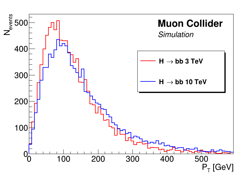
The detector requirements determined for a $\sqrt{s}=3$ TeV MuC case are also fundamental for designing the $\sqrt{s}=10$ TeV detector. Fig. 16 presents the transverse momentum of $b$-quarks from $H\to b\bar{b}$ decay at $\sqrt{s}=3$ and $\sqrt{s}=10$ TeV: it is evident that the distributions are very similar, with a peak around $p_{\mathrm{T}}\sim 100$ GeV. Therefore, for Higgs physics, similar requirements are expected for $\sqrt{s}=3$ TeV and $\sqrt{s}=10$ TeV cases.

Figure 16: Transverse momenta of $b$-quarks from the $H\rightarrow b\bar{b}$ decay, at $\sqrt{s}=3$ and $\sqrt{s}=10$ TeV muon-muon collisions, determined with Madgraph [58].

8 Outlook

The studies presented in this paper demonstrate that at a $\sqrt{s}=3$ TeV MuC, a state-of-the-art detector enables high-precision measurements of Higgs cross sections, including that of double Higgs production. This allows for the determination of the Higgs trilinear self-coupling with an accuracy that surpasses that of the HL-LHC, with only one experiment and 1 ab^-1 of data. The estimates have been performed using a detailed detector simulation, which includes the beam-induced background [21]. For each analysis, the events of the Higgs boson signal and corresponding physics backgrounds have been fully simulated and reconstructed (Sec. 3). The statistical sensitivities on the Higgs cross sections measurements (Sec. 4) for the considered Higgs decay channels ($H\rightarrow b\bar{b}$, $H\rightarrow WW^{*}$, $H\rightarrow ZZ^{*}$, $H\rightarrow\mu^{+}\mu^{-}$, and $H\rightarrow\gamma\gamma$) are consistent with those obtained using parametric detector simulations. This consistency underscores the capability of the detector design and reconstruction algorithms to effectively manage the effects of the beam-induced background. The 3 TeV center-of-mass energy is not optimal for measuring the Higgs width, as indicated by Refs. [51, 50] and the analysis presented here in Sec. 5. The limitation is due to the production mechanism and therefore cannot be overcome.

The estimated precision on the Higgs trilinear self-coupling (discussed in Sec. 6) is currently affected by the performance of the simplified algorithms employed in event reconstruction. The impact of planned improvements have been assessed, bringing the precision to a level compatible with that obtained with the parametric studies in Refs. [13, 10]. This also provides confidence in the prospects obtained in Ref. [13] for a measurement of the trilinear self-coupling at a center-of-mass energy of 10 TeV. Running a MuC at $\sqrt{s}=10$ TeV for 5 years is expected to achieve an uncertainty of approximately 4% with 10 ab^-1, which represents the best precision attainable by any future collider.

Another important outcome of this paper is the determination of detector requirements for Higgs physics (Sec. 7), derived from detailed analyses that utilize various physics objects. These requirements (Tab. 10), found to be applicable also at higher center-of-mass energies, serve as the foundation for detector design.

In fact, the average transverse momentum of particles from Higgs decays is of the same order ($\sim$$100$ GeV) at both $\sqrt{s}=3$ TeV and $\sqrt{s}=10$ TeV [58]. Moreover, the impact of beam-induced background on the detector at $\sqrt{s}=10$ TeV is expected to be similar to that at $\sqrt{s}=3$ TeV [21]. For these reasons, the detector is anticipated to provide the desired performance at the higher center-of-mass energy, where a MuC can achieve a precision on the Higgs sector unreachable by other proposed facilities.

Future work with the detailed detector simulation should consider: the decay channels not yet studied (e.g. $H\to\tau^{+}\tau^{-}$), for the determination of additional Higgs couplings with fermions and bosons; an optimization of the algorithms for the measurement of the trilinear Higgs self-coupling; a first study on the measurement of the quartic self-coupling at $\sqrt{s}=10$ TeV.

References

- \bibcommenthead
- Dawson et al. [2022] Dawson, S., et al.: Report of the Topical Group on Higgs Physics for Snowmass 2021: The Case for Precision Higgs Physics (2022) arXiv:arXiv:2209.07510 [hep-ph]
- Higgs [1964] Higgs, P.W.: Broken symmetries, massless particles and gauge fields. Phys. Lett. 12, 132–133 (1964) https://doi.org/10.1016/0031-9163(64)91136-9
- Higgs [1966] Higgs, P.W.: Spontaneous Symmetry Breakdown without Massless Bosons. Phys. Rev. 145, 1156–1163 (1966) https://doi.org/10.1103/PhysRev.145.1156
- Englert and Brout [1964] Englert, F., Brout, R.: Broken Symmetry and the Mass of Gauge Vector Mesons. Phys. Rev. Lett. 13, 321–323 (1964) https://doi.org/10.1103/PhysRevLett.13.321
- Guralnik et al. [1964] Guralnik, G.S., Hagen, C.R., Kibble, T.W.B.: Global Conservation Laws and Massless Particles. Phys. Rev. Lett. 13, 585–587 (1964) https://doi.org/10.1103/PhysRevLett.13.585
- [6] Narain, M., Reina, L., Tricoli, A., et al.: The Future of US Particle Physics – The Snowmass 2021 Energy Frontier Report https://doi.org/10.48550/arXiv.2211.11084 arXiv:arXiv:2211.11084 [hep-ex]
- LHC Higgs Cross Section Working Group [2013] LHC Higgs Cross Section Working Group: Handbook of LHC Higgs Cross Sections: 3. Higgs Properties (2013) https://doi.org/10.5170/CERN-2013-004 arXiv:arXiv:1307.1347 [hep-ph]
- Aad et al. [2023] Aad, G., et al.: Constraints on the Higgs boson self-coupling from single- and double-Higgs production with the ATLAS detector using pp collisions at TeV. Phys. Lett. B 843, 137745 (2023) https://doi.org/10.1016/j.physletb.2023.137745 arXiv:arXiv:2211.01216 [hep-ex]
- Tumasyan et al. [2022] Tumasyan, A., et al.: A portrait of the Higgs boson by the CMS experiment ten years after the discovery. Nature 607(7917), 60–68 (2022) https://doi.org/10.1038/s41586-022-04892-x arXiv:arXiv:2207.00043 [hep-ex]. [Erratum: Nature 623, (2023)]
- Accettura et al. [2023] Accettura, C., et al.: Towards a Muon Collider. Eur. Phys. J. C 83 (2023) https://doi.org/10.1140/epjc/s10052-023-11889-x arXiv:2303.08533
- [11] Muon Accelerator Program http://map.fnal.gov
- Ali et al. [2022] Ali, H.A., et al.: The muon smasher’s guide. Rep. Prog. Phys. (85), 084201 (2022) https://doi.org/10.1088/1361-6633/ac6678 arXiv:2103.14043
- de Blas et al. [2022] Blas, J., et al.: The physics case of a 3 TeV muon collider stage (2022) arXiv:2203.07261 [hep-ph]
- [14] Palmer, M., et al.: Muon Accelerators for Particle Physics (MUON). https://iopscience.iop.org/journal/1748-0221/page/extraproc46
- Bogomilov et al. [2020] Bogomilov, M., et al.: Demonstration of cooling by the Muon Ionization Cooling Experiment. Nature 578(7793), 53–59 (2020) https://doi.org/10.1038/s41586-020-1958-9 arXiv:arXiv:1907.08562 [physics.acc-ph]
- [16] Intenational Muon Collider Collaboration https://muoncollider.web.cern.ch
- [17] Alexahin, Y., Gianfelice-Wendt, E., Kapin, V.: Muon collider lattice concepts. 2018 JINST 13, 11002 https://doi.org/10.1088/1748-0221/13/11/P11002 arXiv:1806.08717
- [18] Di Benedetto, V., et al.: A study of muon collider background rejection criteria in silicon vertex and tracker detectors. 2018 JINST 13, 09004 https://doi.org/10.1088/1748-0221/13/09/P09004 arXiv:1807.00074
- Mokhov and Striganov [2007] Mokhov, N.V., Striganov, S.I.: MARS15 Overview. AIP Conf. Proc. 896(1), 50–60 (2007) https://doi.org/10.1063/1.2720456
- Ahdida et al. [2022] Ahdida, C., et al.: New Capabilities of the FLUKA Multi-Purpose Code. Front. in Phys. 9, 788253 (2022) https://doi.org/10.3389/fphy.2021.788253
- Lucchesi et al. [2024] Lucchesi, D., et al.: Machine-Detector interface for multi-TeV Muon Collider. PoS EPS-HEP2023, 630 (2024) https://doi.org/10.22323/1.449.0630
- Agostinelli et al. [2003] Agostinelli, S., et al.: Geant4—a simulation toolkit. Nucl. Instrum. Methods A 506(3), 250–303 (2003) https://doi.org/10.1016/S0168-9002(03)01368-8
- [23] Muon Collider Software https://github.com/MuonColliderSoft
- [24] ILC Soft. https://ilcsoft.desy.de/portal
- Forslund and Meade [2022] Forslund, M., Meade, P.: High precision higgs from high energy muon colliders. J. High Energ. Phys. 2022(8), 185 (2022) https://doi.org/10.1007/jhep08(2022)185 arXiv:2203.09425
- Alwall et al. [2014] Alwall, J., et al.: The automated computation of tree-level and next-to-leading order differential cross sections, and their matching to parton shower simulations. JHEP 07, 079 (2014) https://doi.org/10.1007/JHEP07(2014)079 arXiv:arXiv:1405.0301 [hep-ph]
- Kilian et al. [2011] Kilian, W., Ohl, T., Reuter, J.: WHIZARD: Simulating Multi-Particle Processes at LHC and ILC. Eur. Phys. J. C 71, 1742 (2011) https://doi.org/10.1140/epjc/s10052-011-1742-y arXiv:0708.4233
- Sjöstrand et al. [2015] Sjöstrand, T., et al.: An introduction to PYTHIA 8.2. Comput. Phys. Commun. 191, 159–177 (2015) https://doi.org/10.1016/j.cpc.2015.01.024 arXiv:1410.3012
- Bredt et al. [2022] Bredt, P.M., Kilian, W., Reuter, J., Stienemeier, P.: NLO electroweak corrections to multi-boson processes at a muon collider. JHEP 12, 138 (2022) https://doi.org/10.1007/JHEP12(2022)138 arXiv:2208.09438
- Castelli [2022] Castelli, L.: Study of reconstruction and coupling precision determination at Muon Collider. Master’s thesis, University of Padua, Padua, Italy (2022)
- [31] Linssen, L., Miyamoto, A., Stanitzki, M., (editors), H.W.: Physics and Detectors at CLIC: CLIC Conceptual Design Report https://doi.org/10.48550/arXiv.1202.5940 arXiv:arXiv:1202.5940 [physics.ins-det]
- [32] Marlin framework https://ilcsoft.desy.de
- Thomson [2009] Thomson, M.A.: Particle flow calorimetry and the PandoraPFA algorithm. Nucl. Instrum. Methods A 611(1), 25–40 (2009) https://doi.org/10.1016/j.nima.2009.09.009 arXiv:0907.3577
- Brondolin et al. [2020] Brondolin, E., et al.: Conformal tracking for all-silicon trackers at future electron–positron colliders. Nucl. Instrum. Methods A 956, 163304 (2020) https://doi.org/10.1016/j.nima.2019.163304 arXiv:1908.00256
- Billoir and Qian [1990] Billoir, P., Qian, S.: Simultaneous pattern recognition and track fitting by the Kalman filtering method. Nucl. Instrum. Methods A 294(1), 219–228 (1990) https://doi.org/10.1016/0168-9002(90)91835-Y
- Catani et al. [1993] Catani, S., Dokshitzer, Y.L., Seymour, M.H., Webber, B.R.: Longitudinally-invariant -clustering algorithms for hadron-hadron collisions. Nucl. Phys. B 406, 187–224 (1993) https://doi.org/10.1016/0550-3213(93)90166-M
- Da Molin [2021] Da Molin, G.: Study of b- and c- jets identification for Higgs coupling measurement at muon collider. Master’s thesis, University of Padua, Padua, Italy (2021)
- Roe et al. [2005] Roe, B.P., et al.: Boosted decision trees as an alternative to artificial neural networks for particle identification. Nucl. Instrum. Methods A 543(2), 577–584 (2005) https://doi.org/10.1016/j.nima.2004.12.018 arXiv:physics/0408124
- Hoecker et al. [2009] Hoecker, A., et al.: TMVA - Toolkit for Multivariate Data Analysis (2009) arXiv:arXiv:physics/0703039 [physics.data-an]
- Brun and Rademakers [1997] Brun, R., Rademakers, F.: ROOT: An object oriented data analysis framework. Nucl. Instrum. Meth. A 389, 81–86 (1997) https://doi.org/10.1016/S0168-9002(97)00048-X
- Casarsa et al. [2023] Casarsa, M., Lucchesi, D., Sestini, L.: Experimentation at a muon collider (2023) https://doi.org/10.1146/annurev-nucl-102622-011319 arXiv:2311.03280 [hep-ex]
- Montella [2021] Montella, A.: Study of the Physics Potential of the Direct Decay Channel at a 3 TeV Muon Collider. Master’s thesis, University of Trieste, Trieste, Italy (2021)
- de Favereau et al. [2014] Favereau, J., Delaere, C., Demin, P., Giammanco, A., Lemaître, V., Mertens, A., Selvaggi, M.: DELPHES 3: a modular framework for fast simulation of a generic collider experiment. JHEP 02, 057 (2014) https://doi.org/10.1007/JHEP02(2014)057 arXiv:arXiv:1307.6346 [hep-ex]
- Particle Data Group [2022] Particle Data Group: Review of Particle Physics. Prog. Theor. Exp. Phys. 2022, 083–01 (2022) https://doi.org/10.1093/ptep/ptac097
- ATLAS and CMS collaborations [2022] ATLAS and CMS collaborations: Snowmass White Paper Contribution: Physics with the Phase-2 ATLAS and CMS Detectors. ATL-PHYS-PUB-2022-018, CMS PAS FTR-22-001 (2022)
- Bernardi et al. [2022] Bernardi, G., et al.: The Future Circular Collider: a Summary for the US 2021 Snowmass Process (2022) arXiv:arXiv:2203.06520 [hep-ex]
- Aryshev et al. [2022] Aryshev, A., et al.: The International Linear Collider: Report to Snowmass 2021 (2022) arXiv:arXiv:2203.07622 [physics.acc-ph]
- Abramowicz et al. [2017] Abramowicz, H., et al.: Higgs physics at the CLIC electron–positron linear collider. Eur. Phys. J. C 77(7), 475 (2017) https://doi.org/10.1140/epjc/s10052-017-4968-5 arXiv:arXiv:1608.07538 [hep-ex]
- Giambastiani [2024] Giambastiani, L.: Study of Z boson production in association with jets at LHCb and at a future Muon Collider. PhD thesis, University of Padua, Padua, Italy (2024)
- Li et al. [2024] Li, P., Liu, Z., Lyu, K.-F.: Higgs boson width and couplings at high energy muon colliders with forward muon detection. Phys. Rev. D 109(7), 073009 (2024) https://doi.org/10.1103/PhysRevD.109.073009 arXiv:2401.08756 [hep-ph]
- Forslund and Meade [2024] Forslund, M., Meade, P.: Precision Higgs width and couplings with a high energy muon collider. JHEP 01, 182 (2024) https://doi.org/10.1007/JHEP01(2024)182 arXiv:arXiv:2308.02633 [hep-ph]
- Forslund [2022] Forslund, M.: Single Higgs Precision at a Muon Collider. In: Muon Collider Physics and Detector Workshop, Fermilab, Batavia IL, USA (2022)
- Buonincontri [2020] Buonincontri, L.: Study of mitigation strategies of beam-induced background and Higgs boson couplings measurements at a muon collider. Master’s thesis, University of Padua, Padua, Italy (2020)
- Buonincontri [2023] Buonincontri, L.: Search for heavy flavour Higgs boson decays at hadron and future Muon Collider. PhD thesis, University of Padua, Padua, Italy (2023)
- Han et al. [2021] Han, T., et al.: Precision test of the muon-higgs coupling at a high-energy muon collider. JHEP 12, 162 (2021) https://doi.org/10.1007/jhep12(2021)162 arXiv:2108.05362
- [56] Bols, E., et al.: Jet Flavour Classification Using DeepJet. 2020 JINST 15(12), 12012 https://doi.org/10.1088/1748-0221/15/12/P12012 arXiv:arXiv:2008.10519 [hep-ex]
- LHCb collaboration [2023] LHCb collaboration: Performance of new jet techniques based on machine learning for and searches. LHCB-FIGURE-2023-029 (2023)
- Sestini [2024] Sestini, L.: R&D towards the detector for the Muon Collider. PoS EPS-HEP2023, 552 (2024) https://doi.org/10.22323/1.449.0552