A quantum implementation of high-order power method for estimating geometric entanglement of pure states

Abstract

Entanglement is one of the fundamental properties of a quantum state and is a crucial differentiator between classical and quantum computation. There are many ways to define entanglement and its measure, depending on the problem or application under consideration. Each of these measures may be computed or approximated by multiple methods. However, hardly any of these methods can be run on near-term quantum hardware. This work presents a quantum adaptation of the iterative higher-order power method for estimating the geometric measure of entanglement of multi-qubit pure states using rank-1 tensor approximation. This method is executable on current (hybrid) quantum hardware and does not depend on quantum memory. We study the effect of noise on the algorithm using a simple theoretical model based on the standard depolarising channel. This model allows us to post hoc mitigate the effects of noise on the results of the computation.

1 Introduction

For a quantum algorithm to provide advantage over a classical alternative, entanglement [1] is a necessary ingredient. Not only the presence but the “degree” of entanglement in a quantum state is an important property for many applications [2], for example quantum information technologies [3], quantum teleportation and quantum communication [1] and quantum cryptography [4]. On the one hand, if there is not “enough” entanglement a quantum circuit can be efficiently simulated by classical devices [5]. On the other hand, some systems with “maximally” entangled states, such as stabilizer codes [6], admit efficient classical simulations [7, 8]. Also, highly entangled states are not useful as computational resources in the measurement based computing paradigm [9]. In the setting of parameterised quantum circuits, entanglement contributes to “barren plateaus” in the cost function landscape that make training a challenge [10, 11].

Consequently, there has been an effort to define and quantify [2] entanglement with different methods [12] being favoured depending on the application. Some definitions, (for example, quantum mutual information or von Neumann entropy [1]) are measures of bipartite entanglement only and are computationally expensive for mixed states. Others, such as concurrence [13], have no unique definition for higher ($>2$) dimensional systems [14, 15]. In fact, the very concept of $n$-partite (multi-qubit) entanglement is still not clearly understood [16].

The geometric measure of entanglement ($E_{G}$) [17, 18, 19] is a popular multi-partite entanglement metric with a clear geometric interpretation, which naturally extends to the $n$-partite case and to mixed states [19]. Geometric entanglement is, among other applications, useful to define entanglement witnesses [19] which are used as a positive indicator of entanglement for a subset of quantum states.

The first algorithm to compute $E_{G}$ used it (under the name of “the Groverian measure of entanglement”) to assess the probability of success for an initial state in Grover’s Algorithm [20, 21]. This method was rephrased in terms of eigenvalues and Singular Value Decomposition (SVD) and extended for mixed states [22]. A similar method was formulated in terms of Tucker decomposition [23] using the Higher Order Orthogonal Iteration (HOOI) algorithm [24]. A parallel strand of work [25, 26], based on the fundamental connection between geometric entanglement and tensor theory, introduced a series of algorithms to approximate $E_{G}$ [27, 28, 29]. These approaches can be considered as generalizations of the popular power methods (e.g. the Lanczos method and Arnoldi iterations) used for studying the eigenvalues of matrices (for example see [30]).

With accessible quantum hardware, measuring entanglement on a physical device becomes a problem of interest. The algorithms mentioned above are all intended to be executed on classical machines. Naïvely, we would have to do full-state tomography to reconstruct the quantum state in a classical computer to calculate its entanglement. As the number of qubits increases the amount of measurements required for tomography rises exponentially. Alternatively, if we know the quantum state in advance we can prepare the appropriate entanglement witness [3]. However, the latter method does not allow one to get the measure of entanglement itself. Recently variational quantum circuits (VQC) have been suggested to compute geometric entanglement of pure states on a quantum computer [31, 32]. VQC algorithms, unfortunately, suffer from “barren plateaus” [10, 11] which hinders the scalability of the approach.

In this paper, we present an iterative quantum algorithm for computing the geometric entanglement of pure quantum states. The algorithm is a quantum adaptation of the Higher Order Power Method (HOPM) [24] for estimating Rank-1 Tensor Approximation (RTA). We show how to implement crucial steps of HOPM in the quantum domain and analyse their robustness w.r.t. noise. Our aim is to measure entanglement on near-term quantum devices more time efficiently than full-state tomography and more space efficiently (qubits vs classical memory) than executing HOPM on a classical device.

Our paper is structured as follows. First, we formally define geometric entanglement and its connection to RTA and recall the HOPM algorithm for this problem. Next, we present our quantum implementation of HOPM. Then we show some simulation results exploring the robustness of the algorithm to noise and discuss some simple ways to mitigate it. Finally, we discuss some future directions and unresolved questions.

2 Results

2.1 Preliminaries: Geometric Entanglement in terms of rank-1 tensor approximation

Definition 1 (Fully separable and entangled states).

Let $\mathbb{H}^{n}$ be an $n$-qubit Hilbert space. A pure $n$-partite state $\ket{\phi}\in\mathbb{H}^{n}$ is fully separable if and only if it is a product state of 1-qubit states $\ket{{\bf v}_{i}}\in\mathbb{H}$ [1]:

$$\ket{\phi}=\ket{{\bf v}_{1}}\otimes\cdots\otimes\ket{{\bf v}_{n}}.$$ (1)

We say an $n$-partite pure state is entangled if it is not fully separable. Let $S_{n}\subseteq\mathbb{H}^{n}$ denote the set of fully separable states.

Definition 2 (Geometric measure of entanglement [17, 18, 19]).

Let the geometric measure of entanglement of a pure state $\ket{\psi}$ be

$$E_{G}(\ket{\psi})=1-\max_{\ket{\phi}\in S_{n}}|\langle\phi|\psi\rangle|^{2},$$ (2)

where $\tilde{\lambda}=\max\limits_{\ket{\phi}\in S_{n}}|\langle\phi|\psi\rangle|$ is called the entanglement eigenvalue.

One approach to compute the value of $\tilde{\lambda}$ is to solve the problem of finding the “closest” fully separable state (CSS) $\ket{\phi}$ to the state $\ket{\psi}$. CSS is formally stated as a minimization problem over $\ket{\phi}\in S_{n}$ with the objective function being the distance between $\ket{\psi}$ and $\ket{\phi}$:

$$\min_{\ket{\phi}\in S_{n}}d(\ket{\psi},\ket{\phi}),$$ (3)

where $d(a,b)=\|a-b\|_{F}$ is the reference distance with $a,b\in\mathbb{H}^{n}$ and $\|\cdot\|_{F}$ being the Frobenius norm (we will omit the subscript $F$ in what follows). We note that the minimizer of Eq. (3) exists (but may not be unique) since the set of fully separable states $S_{n}$ is the classical Segre variety [33, 34, 35], which is closed in Zariski and Euclidean topology when defined over the complex numbers. Minimizing the distance from a variety is a problem well studied from different perspectives, for example in the context of algebraic geometry the concept of Euclidean Distance Degree has been introduced [36]. In the present work we deal with the minimization of Eq. (3) in terms of a system of nonlinear equations with $\lambda$ being a Lagrange multiplier (see [26, 19, 29]):

$$T_{\psi}\times_{\hat{i}}\left({\bf v}_{1}^{\ast},\ldots,{{\bf v}_{i-1}^{\ast}},{\bf v}_{i+1}^{\ast},\ldots,{\bf v}_{n}^{\ast}\right)=\lambda{\bf v}_{i},$$ (4)

$$T_{\psi}^{*}\times_{\hat{i}}\left({{\bf v}_{1}},\ldots,{{\bf v}_{i-1}},{{\bf v}_{i+1}},\ldots,{{\bf v}_{n}}\right)=\lambda{\bf v}_{i}^{\ast},$$

$$\|{\bf v}_{i}\|=\sum_{b_{i}}|v_{i,b_{i}}|^{2}=1,\quad i\in\{1,\ldots,n\}$$

$$\lambda\in\mathbb{R},$$

where $T_{\psi}\in\mathbb{C}_{2}^{\otimes n}$ ($\mathbb{C}_{2}=\mathbb{C}\times\mathbb{C}$ is a two-dimensional complex vector space) is a tensor representation of $\ket{\psi}$ in the basis $\ket{b_{1},\ldots,b_{n}}=\otimes_{i}\ket{b_{i}}$ with components $\psi_{b_{1},\ldots,b_{n}}\in\mathbb{C}$ defined as:

$$\ket{\psi}=\sum_{b_{1},\ldots,b_{n}}\psi_{b_{1},\ldots,b_{n}}\ket{b_{1},\ldots,b_{n}},$$

and ${\bf v}_{i}=(v_{i,0},v_{i,1})^{\rm T}\in\mathbb{C}_{2}$ is a vector of components of the one-qubit states $\ket{{\bf v}_{i}}$, defined in Eq. (1), in the same basis; the asterisk means complex conjugate; the symbol $\times_{\hat{i}}$ is $n$-mode vector product over all modes except the $i$-th one, which is a contraction of a tensor on the left with the tuple of vectors on the right, skipping the $i$-th index (mode) of the tensor (when the subscript is not given none of the modes are skipped). In tensor analysis, the problem of finding a solution to a system of equations such as Eq. (4) is usually referred to as the $U$-eigenpair problem for the tensor $T_{\psi}$. One way to solve this problem is by using RTA [26, 29].

The problem of RTA for a particular tensor is $\mathsf{NP}$-hard [37] and so exact or global techniques such as homotopy continuation methods [38] may take exponential time or fail to converge. Alternatively, approximate techniques may run quickly but may return a local minima. Some of the well-known algorithms that can be used for approximating RTA are Higher-Order Singular Value Decomposition (HOSVD) [39], HOPM and HOOI [24]. In the particular case of tensors representing the pure quantum state of a finite system of qubits, both HOSVD and HOOI simplify to the HOPM algorithm, which is based upon the Alternating Least Squares (ALS) approach [24, 40] for solving non-linear systems of equations.

The application of HOPM to the first sub-system of equations in Eq. (4) is presented in pseudocode in Algorithm 1. (Note, that this is a known technique [24, 22, 26, 28, 29]).

Algorithm 1 HOPM algorithm for estimating RTA of $T_{\psi}$ with absolute accuracy $\epsilon$ [24].

HOPM$T_{\psi}$, $\epsilon$

1:Let $(\mathbf{v}_{1}^{(0)},\ldots,\mathbf{v}_{n}^{(0)})$ be a tuple of some $n$ one-qubit state vectors

2:initialise $k$ to $0$ $\mid\lambda^{(k+1)}-\lambda^{(k)}\mid\ >\epsilon$ $i\in{1,\ldots,n}$

3:

4:${\bf u}^{(k+1)}_{i}=T_{\psi}\times_{\hat{i}}\left({{\bf v}^{(k+1)^{\ast}}_{1}},\ldots,{{\bf v}^{(k+1)^{\ast}}_{i-1}},{\bf v}^{(k)^{\ast}}_{i+1},\ldots,{\bf v}^{(k)^{\ast}}_{n}\right)$

5:

6:${\bf v}^{(k+1)}_{i}={\bf u}^{(k+1)}_{i}/\|{\mathbf{u}}_{i}^{(k+1)}\|$

7:

8:$\lambda^{(k+1)}=\left|T_{\psi}\times\left({{\bf v}^{(k+1)^{\ast}}_{1}},\ldots,{\bf v}^{(k+1)^{\ast}}_{n}\right)\right|$

9:

10:increment $k$ $\lambda^{(k+1)}$ and $(\mathbf{v}_{1}^{(k+1)},\ldots,\mathbf{v}_{n}^{(k+1)})$

Remark 3.

The global phase of $\ket{{\bf v}_{i}}$ and the chosen computational basis do not affect the result for $\lambda$ and convergence of Algorithm 1.

Indeed from line 8 of Algorithm 1 it is evident that global phase prefactors $e^{i\alpha_{j}}$ ($\alpha_{j}\in\mathbb{R}$) of ${{\bf v}^{(k)}_{j}}$ do not affect the result $\lambda$ of the algorithm on any iteration $k$. From the same line we see that the change of basis does not change $\lambda$, since the inner product of $T_{\psi}$ with all the vectors ${\bf v}_{i}$ on $k$-th iteration is basis invariant. This also means that the convergence of the algorithm, which is determined by $\lambda$ (see line 2), is also not affected.

2.2 Quantum implementation of HOPM for estimating the entanglement eigenvalue

In this section we present an iterative quantum algorithm, which is a HOPM approach for approximating RTA with its crucial steps (lines 4-8 in Algorithm 1) performed on a quantum device. We will refer to this algorithm as QHOPM. The input for the algorithm is an $n$-qubit quantum circuit $U_{\psi}$ that prepares the target state $\ket{\psi}=U_{\psi}\ket{\bf 0}\in\mathbb{H}^{n}$, where $\ket{\bf 0}=\ket{0}^{\otimes n}$ is the initial state of the system. The separable state $\ket{\phi}\in S_{n}$ is encoded as a tensor product of one-qubit $x$ and $z$ rotations acting on $\ket{\bf 0}$:

$$\ket{\phi}=\bigotimes_{i=1}^{n}\ket{{\bf v}_{i}}=\bigotimes_{i=1}^{n}R_{z}(\varphi_{i})R_{x}(\vartheta_{i})\ket{\bf 0},$$ (5)

where $\ket{\mathbf{v}_{i}}$ are one-qubit states and $\vartheta\in[0,\pi),\varphi\in[0,2\pi)$. This choice of encoding of $\ket{\mathbf{v}_{i}}$ differs from any other encoding only by global phase and therefore is valid due to Remark 3. We choose an initial separable state $\ket{\phi^{(0)}}$ by randomly choosing the angles $(\vartheta_{i}^{(0)},\varphi_{i}^{(0)})$ as a starting point for the approximation.

The first key steps of Algorithm 1 are lines 4 and 6 (consisting of the $n$-mode product and normalization) which yield an updated version of $\ket{\mathbf{v}_{i}}$.

& n V_i^(k) = & R_x(ϑ_1^(k)) R_z(φ_1^(k))
n ⋮ n n
R_x(ϑ_i-1^(k)) R_z(φ_i-1^(k))

R_x(ϑ_i+1^(k-1)) R_z(φ_i+1^(k-1))
n ⋮ n n
R_x(ϑ_n^(k-1)) R_z(φ_n^(k-1))

Figure 1: Circuit representation of a separable state used for the $i$th mode update. The sub-circuit implements $V_{i}^{(k)}$ (see Eq. (8)), the vector part of the $n$-mode vector product for line 4 of Algorithm 1.

Proposition 4.

Lines 4 and 6 of Algorithm 1 for the state $\ket{\psi}=U_{\psi}\ket{\bf 0}$ at any iteration $k>0$ are equivalent, up to a global phase, to the following update of $\ket{\mathbf{v}_{i}^{(k+1)}}$:

$$\ket{{\bf v}_{i}^{(k+1)}}=\sum_{b}v_{i,b}^{(k+1)}\ket{b}=\frac{\sum_{b}u_{i,b}^{(k+1)}\ket{b}}{\sqrt{\sum_{b}|u_{i,b}^{(k+1)}|^{2}}},$$ (6)

where

$$u_{i,b}^{(k+1)}=\left(\bra{0}^{\otimes(n-i)}\otimes\bra{b}\otimes\bra{0}^{\otimes(i-1)}\right){V_{i}^{(k+1)}}^{\dagger}U_{\psi}\ket{\bf 0}$$ (7)

is the $b$-th component of the $n$-mode vector product in line 4 having

$$\begin{split}V_{i}^{(k+1)}=&\left[\bigotimes_{l=i+1}^{n}R_{z}(\varphi_{l}^{(k+1)})R_{x}(\vartheta_{l}^{(k+1)})\right]\\ &\otimes I\otimes\\ &\left[\bigotimes_{l=1}^{i-1}R_{z}(\varphi_{l}^{(k)})R_{x}(\vartheta_{l}^{(k)})\right],\end{split}$$ (8)

(see Fig. 1) and $\ket{b}$ is a one-qubit computational basis.

Proof.

We start with line 4 Algorithm 1 where we calculate the updated ${\bf u}_{i}^{(k)}$, the $b$-th component of which is

$$u_{i,b}^{(k+1)}=T_{\psi}\times\left({\textbf{v}_{1}^{(k+1)}}^{\ast},\ldots,{\textbf{v}_{i-1}^{(k+1)}}^{\ast},{\bf e}^{\ast}_{b},{\textbf{v}_{i+1}^{(k)}}^{\ast},\ldots,{\textbf{v}_{n}^{(k)}}^{\ast}\right),$$

where ${\bf e}_{b}$ is a one-qubit basis vector for the $b$-th component. Let us substitute to the right-hand side the following expressions for the components of $T_{\psi}$ and ${\bf v}_{m\neq i}^{(k)}$ in terms of $U_{\psi}$ and $R_{z}R_{x}$:

$$\psi_{l_{1},...,l_{n}}=\bra{l_{1}...l_{n}}U_{\psi}\ket{\bf 0};\quad v_{m,l}^{(k)}=\bra{l}R_{z}(\varphi_{m}^{(k)})R_{x}(\vartheta_{m}^{(k)})\ket{0},$$

and taking into account that the $l$-th component of ${\bf e}_{b}$ in bra-ket notation is $\bra{l}b\rangle$, we get for the $b$-th component of $\textbf{u}_{i}^{(k+1)}$

$$\begin{split}u_{i,b}^{(k+1)}=&\sum_{l_{1},...,l_{n}}\bra{0}R_{x}^{\dagger}(\vartheta_{1}^{(k+1)})R_{z}^{\dagger}(\varphi_{1}^{(k+1)})\ket{l_{1}}...\langle b\ket{l_{i}}...\\ &\bra{0}R_{x}^{\dagger}(\vartheta_{n}^{(k)})R_{z}^{\dagger}(\varphi_{n}^{(k)})\ket{l_{n}}\bra{l_{1}...l_{n}}U_{\psi}\ket{0}\\ =&\left(\bra{0}^{\otimes(n-i)}\otimes\bra{b}\otimes\bra{0}^{\otimes(i-1)}\right){V_{i}^{(k+1)}}^{\dagger}U_{\psi}\ket{\bf 0},\end{split}$$

where $V_{i}^{(k+1)}$ is defined by Eq. (8). This expression corresponds to Eq. (7).

To prove that Eq. (7) yields line 4 of Algorithm 1 we perform the above steps in reverse, taking into account Remark 3.

Note, that for the components defined by (7) to correspond to a proper quantum state, they need to be normalized:

$$\ket{{\bf v}_{i}^{(k+1)}}=\frac{\sum_{b}u_{i,b}^{(k+1)}\ket{b}}{\sqrt{\sum_{b}|u_{i,b}^{(k+1)}|^{2}}},$$

which corresponds to the line 6 of Algorithm 1. ∎

Proposition 4 allows us to understand which type of operations and measurements we should perform to implement lines  4 and 6 of the algorithm, in particular, we need to be able to measure $u_{i,b}^{(k+1)}$ and obtain the updated pair of angles $(\vartheta_{i}^{(k+1)},\varphi_{i}^{(k+1)})$ for further encoding the updated $\ket{{\bf v}_{i}^{(k+1)}}$.

2.2.1 Recovering one-qubit states with tomography

From Eq. (7) it is evident that the components of $\ket{{\bf v}_{i}^{(k)}}$ should be obtained under the condition that all the qubits except the $i$-th one are projected on the state $\ket{0}$. Thus, to obtain the angles $(\vartheta_{i}^{(k)},\varphi_{i}^{(k)})$ for the one-qubit state encoding of $\ket{{\bf v}_{i}^{(k)}}$ (see Eq. (5)) it is sufficient to solve the following system of equations:

$$P_{i}(0)=\cos^{2}(\vartheta/2);$$ (9)

$$\langle X_{i}\rangle=P_{i}(-)-P_{i}(+)=\sin\vartheta\sin\varphi;$$

$$\langle Y_{i}\rangle=P_{i}(+i)-P_{i}(-i)=-\sin\vartheta\cos\varphi,$$

where $X_{i}=\Pi_{0}^{\otimes(n-i)}\otimes X\otimes\Pi_{0}^{\otimes(i-1)}$ and $Y_{i}=\Pi_{0}^{\otimes(n-i)}\otimes Y\otimes\Pi_{0}^{\otimes(i-1)}$ with $\Pi_{0}=\ket{0}\bra{0}$ being projector on the state $\ket{0}$; the function

$$P_{i}(s)=|\langle s\ket{{\bf v}_{i}^{(k)}}|^{2}=|v_{i,s}^{(k)}|^{2}=\frac{|u_{i,s}^{(k)}|^{2}}{\sum_{b\in B_{s}}|u_{i,b}^{(k)}|^{2}}$$ (10)

is a probability of the $i$-th qubit being in the state $\ket{s}=U_{s}\ket{0}\in B_{s}$ after the measurement, whilst all other qubits are in the state $\ket{0}$, with $B_{s}=\{\ket{s},\ket{s}^{\perp}\}$ being a set of one-qubit orthonormal basis states and $u_{i,j}^{(k)}$ defined by Eq. (7).

To obtain these probabilities we need to measure $u_{i,s}^{(k)}$ for the basis vectors $\ket{s}\in\{\ket{0},\ket{1},\ket{+},\ket{-},\ket{-i},\ket{+i}\}$. Post-selection can be used for this, however, the number of samples required to get an acceptable estimate of probability grows exponentially with the number of qubits.

Another method of measuring $u_{i,s}^{(k)}$ can be built upon the well-known Hadamard test procedure [41] as follows.

1. Introduce an ancilla qubit, initialized in the state $\ket{+}=H\ket{0}$, whilst the working (data) qubits are initialized in the ground state $\ket{\bf 0}$.

2. Perform a unitary operation $W={V_{i}^{(k)}}^{\dagger}U_{\psi}$ on the working qubits controlled by the ancilla qubit.

3. Perform a unitary operation $U_{s}^{\dagger}$ on the $i$-th qubit controlled by the ancilla qubit.

4. Measure $\langle X\rangle_{a}$ and $\langle Y\rangle_{a}$ on the ancilla qubit, and calculate $|u_{i,s}^{(k)}|^{2}=\langle X\rangle_{a}^{2}+\langle Y\rangle_{a}^{2}$.

The circuit representation of these steps is given in Fig. 2(b). This approach allows us to obtain each of the required probabilities by measuring six quantities, $P_{i}(s)$, for any number of qubits, however it requires one to be able to implement the controlled $U_{\psi}$ and $V_{i}$, which might be hard on the current generation of quantum devices for some cases of $\ket{\psi}$ and large qubit systems.

In the following text we refer to this whole procedure as one-qubit tomography $\mathcal{T}_{i}$ for the $i$-th qubit on the given $n$-qubit state $\ket{\mu}=W\ket{\bf 0}$:

$$\mathcal{T}_{i}: \mathbb{H}^{n}\to[0,\pi)\times[0,2\pi)$$

$$\ket{\mu}\mapsto(\vartheta,\varphi).$$

2.2.2 Measuring Entanglement

At the end of each iteration $k$, we need to measure $\lambda^{(k)}$.

Remark 5.

Line 8 of Algorithm 1 for a target state $\ket{\psi}=U_{\psi}\ket{\bf 0}$ at any $k>0$ iteration is equivalent to:

$$\lambda^{(k)}=|\bra{\bf 0}{V^{(k)}}^{\dagger}U_{\psi}\ket{\bf 0}|,$$ (11)

where

$$V^{(k)}=\bigotimes_{i=1}^{n}R_{z}(\varphi_{i}^{(k)})R_{x}(\vartheta_{i}^{(k)}).$$ (12)

Indeed, using the same procedure as in Proposition 4 we find:

$$\lambda^{(k)}=|\bra{\bf 0}{V^{(k)}}^{\dagger}U_{\psi}\ket{\bf 0}|.$$

From this Remark we see that $\lambda^{(k)}$ is obtained by measuring $v_{i,0}^{(k)}$ using the procedure described in Section 2.2.1 with $W={V^{(k)}}^{\dagger}U_{\psi}$ (see Fig. 2(b)). We will denote this operation as

$${\Lambda}: \mathbb{H}^{n}\to[0,1]$$

$$\ket{\mu}\mapsto\lambda.$$

By combining the classical Algorithm 1 with the quantum operations above and making use of one-qubit tomography we execute the most memory-intensive operations (contractions of a tensor of size $2^{n}$) of Algorithm 1 in the quantum domain using $n$ qubits; these steps are given in Algorithm 2. The main steps of the algorithm implementation (lines 4 and 8 in Algorithm 2) are summarized in Fig. 2. The result is summarised in Theorem 6.

Algorithm 2 Iterative quantum implementation of Algorithm 1.

QHOPM$U_{\psi}$, $\epsilon$

1:Choose $(\vartheta^{(0)}_{i},\varphi^{(0)}_{i})\in[0,\pi)\times[0,2\pi)$ for $i=1,\ldots,n$

2:initialise $k$ to $0$ $|\lambda_{n}^{(k+1)}-\lambda_{n}^{(k)}|>\epsilon$ $i\in{1,\ldots,n}$

3:$\varphi_{i}^{(k+1)},\vartheta_{i}^{(k+1)}=\mathcal{T}_{i}({V_{i}^{(k+1)}}^{\dagger}U_{\psi}\ket{\bf 0})$

4:$\lambda^{(k+1)}=\Lambda({V^{(k+1)}}^{\dagger}U_{\psi}\ket{\bf 0})$

5:increment $k$ $\lambda^{(k+1)}$ and $\{(\vartheta^{(k+1)}_{i},\varphi^{(k+1)}_{i})\}_{i=1\ldots n}$

$\ket{+}$ & 1 3 2 X, Y
$\ket{0}$ (i-1) [3]U_ψ [3]V_i^(k)^†
$\ket{0}$ U_s^†
$\ket{0}$ (n-i)

(a)

$\ket{+}$ & 1 1 X, Y
$\ket{0}$ n [1]U_ψ [1]V^(k)^†

(b)

Figure 2: Circuit representations of the main steps of QHOPM for the $k$-th iteration. (a) one-qubit tomography for measuring $u_{i,s}^{(k)}$ (see Sec. 2.2.1); (b) measuring $\lambda^{(k)}$. The meter labels show the operators to measure.

Theorem 6.

Given a representation of a quantum circuit $U_{\psi}$ of a target state $\ket{\psi}$ and a sufficiently small $\epsilon$, QHOPM (Algorithm 2) returns a pair $\lambda$ and $\{(\vartheta_{i},\varphi_{i})\}_{i=1\ldots n}$. Here $\{(\vartheta_{i},\varphi_{i})\}_{i=1\ldots n}$ are the parameters of the encoding of a separable state $\ket{\phi}$. These values obey the following conditions:

1. $\ket{\phi}$ is a rank-1 tensor approximation of $\ket{\psi}$.

2. $\lambda=|\langle\phi|\psi\rangle|$ is an approximation of the entanglement eigenvalue of $\ket{\psi}$.

Proof.

First, we note that HOPM (Algorithm 1) satisfies points 1 and 2 of the theorem for the components $T_{\psi}$ of the state $\ket{\psi}$ and one-qubit components $\mathbf{v}_{i}$ of $\ket{\phi}$. Thus, to prove the points 1 and 2 for QHOPM it is enough to prove the equivalence of lines 4-8 of Algorithm 1 to lines 3 and 4 of Algorithm 2.

First, let us prove the equivalence of lines 4 and 6 of HOPM to line 3 of QHOPM. Having the encoding of the state $\ket{\mathbf{v}_{i}^{(k+1)}}$ in terms of the angles $(\vartheta_{i}^{(k+1)},\varphi_{i}^{(k+1)})$, obtained in line 3 of QHOPM, we reconstruct the result of lines 4 and 6 of HOPM up to a global phase as follows, due to Proposition 4, Eq. (5) and Remark 3:

$$v_{i,b}^{(k+1)}=\langle b|\mathbf{v}_{i}^{(k+1)}\rangle=\bra{b}R_{z}(\varphi_{i}^{(k+1)})R_{x}(\vartheta_{i}^{(k+1)})\ket{0}.$$ (13)

To show the other direction, having the components $v_{i,b}^{(k+1)}$, obtained in lines 4 and 6 of HOPM, we solve the system of equations (9) and recover the angles $(\vartheta_{i}^{(k+1)},\varphi_{i}^{(k+1)})$. This proves the equivalence of lines 4-6 of HOPM to line 3 of QHOPM. This result does not depend upon $i$ or $k$, thus, it is valid for any $i$ and $k$.

In Remark 5 we showed how to use the obtained angles $(\vartheta_{i}^{(k+1)},\varphi_{i}^{(k+1)})$ to calculate $\lambda^{(k+1)}$, which is just a way to rewrite line 8 of HOPM using $U_{\psi}$ and $V^{(k+1)}$. The measurement of $\lambda^{(k+1)}$ is denoted as $\Lambda({V^{(k+1)}}^{\dagger}U_{\psi}\ket{\bf 0})$, which is line 4 of QHOPM. This shows the equivalence of line 8 of HOPM to line 4 of QHOPM for any $k>0$ and finishes the proof. ∎

2.2.3 Algorithm Complexity

Recall that $n$ is the number of qubits in the input quantum circuit $U_{\psi}$ that defines the target state $\ket{\psi}$. Assuming the use of the Hadamard test for the $n$-qubit target state $\ket{\psi}$, QHOPM requires $n+1$ qubits.

Each application of the tomography step at line 3 of Algorithm 2 requires $12$ measurements (4 measurements each for $X$, $Y$, and $Z$); and each estimation of the scalar product at line 4 of Algorithm 2 requires $2$ measurements. Thus, each iteration of the loop in line 2 requires $12n+2$ measurements. Each measurement (assuming the Hadamard test) requires $\mathsf{O}\left(\epsilon^{-2}\right)$ single-shot readouts due to the Chernoff bound for absolute error $\epsilon$. The total shot complexity of each iteration is $\mathsf{O}\left(n\epsilon^{-2}\right)$.

The depth of the circuit used for measurements is defined by the depth of the circuit $U_{\psi}$ plus a constant. The constant is the sum of the depth of the separable state encoding ($V_{i}^{(k)}$ or $V^{(k)}$) and the overhead caused by the Hadamard test.

QHOPM is a direct quantum implementation of the classical HOPM algorithm and so has the same convergence properties in the complex domain [26, 29]. However, the rate of convergence has only been shown for real tensors [42, 43, 44]. To our knowledge there is no such analysis for the complex case.

2.3 Simulation Results

In this section, we simulate our algorithm to evaluate its robustness to noise using the IBM Qiskit [45] platform (see Methods section for simulation details). We also show how to mitigate the effects of noise on the algorithm. We refer to the target states by the notation State[$n$] for $n$ qubits, for example GHZ[$9$] is the GHZ state with 9 qubits and Random[$3$] is a particular random state with 3 qubits.

To demonstrate the convergence of the algorithm for different initial separable states we run each simulation with 10 random initial separable states. We then analyse $\overline{E}_{G}$, the average $E_{G}$ for the final 5 algorithm iterations over all initial separable states, and its standard deviation $\sigma_{E_{G}}$.

We begin by verifying that our quantum implementation matches the classical algorithm without noise. We use the GHZ[$9$] state, which has a known $\widetilde{E}_{G}=0.50$, as an example. In Fig. 3(a) we see a good correspondence with classical HOPM, that is QHOPM converges to the same value ($\overline{E}_{G}\approx 0.50$, $\sigma_{E_{G}}\approx 2.8\times 10^{-4}$) as classical HOPM ($\overline{E}_{G}=0.50$). Here we are using $1\times 10^{7}$ shots per measurement yielding an expected error of $\epsilon\approx 3.2\times 10^{-4}$.

In Fig. 3(b) we reduced the number of shots to $1\times 10^{5}$ and we see convergence to the same value $\overline{E}_{G}\approx 0.50$, but with slightly higher $\sigma_{E_{G}}\approx 8\times 10^{-3}$. Notice, that the distribution of $E_{G}$ values found after 1 iteration by QHOPM is different than that found by HOPM for the same initial separable states. By the second iteration HOPM and QHOPM converge to the same values. This divergence (from our experience) is normally not so noticeable, but of all the states we have studied (see Methods for the list of studied states), this effect is most pronounced in $GHZ[9]$. We assume that resolution errors, due to the reduced number of shots in the measurements, are amplified cumulatively for certain states (GHZ[$9$], in particular) during one-qubit tomography resulting in a different (but still improved) separable state from what HOPM or QHOPM with infinite resolution would find. From this point on we proceed with $1\times 10^{5}$ shots for all simulations, since it gives a sufficiently good convergence w.r.t. classical HOPM.

We then introduced depolarising noise (DN) (see Methods) with error rate $p=0.01$. The effects of DN are seen in Fig. 3(c) where the quantum algorithm still managed to converge with little variance ($\sigma_{E_{G}}\approx 0.009$), however, the value that it converged to ($\overline{E}_{G}\approx 0.678$) is greater than the true value ($\widetilde{E}_{G}=0.50$).

Figure 3: Simulation results for QHOPM approximating $E_{G}$ of $GHZ[9]$ in contrast to HOPM. (a) no noise with $1\times 10^{7}$ shots per measurement; (b) no noise with $1\times 10^{5}$ shots per measurement; (c) depolarizing noise, applied to all the gates with $p=0.01$. The mean geometric entanglement ($E_{G}$) for the fixed 10 random initial separable states per iteration of an algorithm is shown by lines. The shaded areas indicate the standard deviations. For the quantum simulations, individual values are marked with $\times$. All the simulations were run for $1\times 10^{5}$ shots per measurement.

To explore the relationship between DN error rate $p$ and the divergence of QHOPM’s $E_{G}$ value from HOPM’s, we ran simulations with $p\in\{0.001,0.01,0.05\}$ representing acceptable, bad and terrible levels of noise, respectively. Again we used GHZ[$9$] as the target state. In Fig. 4(a) we see that when $p=0.001$ the convergence of QHOPM is only slightly off ($\overline{E}_{G}\approx 0.520,\sigma_{E_{G}}\approx 0.011$). The upper limit of error rate that is considered acceptable at this early stage of quantum computing is $p=0.01$, at this level the noise is causing our algorithm to converge to the value $\overline{E}_{G}\approx 0.678$ with $\sigma_{E_{G}}\approx 0.009$. At $p=0.05$ the algorithm still converges with similar variance as before ($\sigma_{E_{G}}\approx 0.005$) but to the incorrect value $\overline{E}_{G}\approx 0.946$.

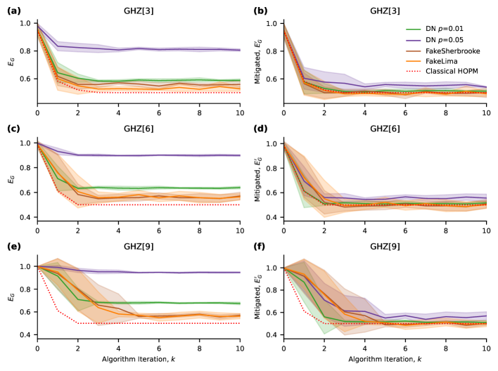
Figure 6: Simulation and mitigation results for the QHOPM algorithm on GHZ states. Row (a) (b) show GHZ[$3$], (c) (d) show GHZ[$6$], (e) (f) show GHZ[$9$]. Column (a) (c) (e) shows the effect of noise on convergence. Column (b) (d) (f) shows the effects of mitigation on the noisy simulation. Each simulation was run 10 times (with the same 10 random initial separable states) with $1\times 10^{5}$ shots per each measurement. Solid lines represent the mean geometric entanglement, $E_{G}{}$, and the lightly shaded colours represent the standard deviation. The colour of the lines represents the noise model used for the simulation (see legend). Red dotted lines show results of classical HOPM.

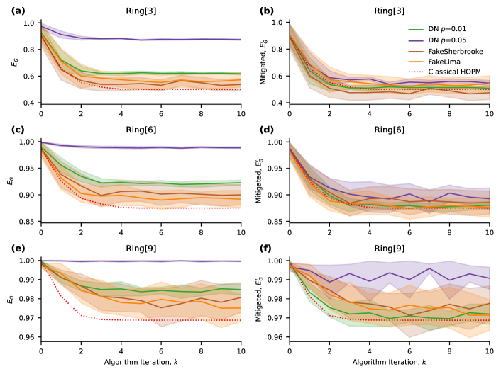
Figure 8: Simulation and mitigation results for the QHOPM algorithm on Ring states. Row (a) (b) show Ring[$3$], (c) (d) show Ring[$6$], (e) (f) show Ring[$9$]. Column (a) (c) (e) shows the effect of noise on convergence. Column (b) (d) (f) shows the effects of mitigation on the noisy simulation. Each simulation was run 10 times (with the same 10 random initial separable states) with $1\times 10^{5}$ shots per each measurement. Solid lines represent the mean geometric entanglement, $E_{G}{}$, and the lightly shaded colours represent the standard deviation. The colour of the lines represents the noise model used for the simulation (see legend). Red dotted lines show results of classical HOPM.

We also examine the state Random[$6$] (see Methods) where we do not know the true $E_{G}$ value. Classical HOPM converges to the value $\overline{E}_{G}\approx 0.639$. With low noise ($p=0.001$) QHOPM converges to $\overline{E}_{G}\approx 0.659,\sigma_{E_{G}}\approx 0.012$, within $\epsilon\approx 0.02$ w.r.t. the classical algorithm’s result. Again, we see that as noise increases, the converged value increases: for $p=0.01$ it goes to $\overline{E}_{G}\approx 0.787$ with $\sigma_{E_{G}}\approx 0.011$, and for $p=0.05$ it goes to $\overline{E}_{G}\approx 0.978$ with $\sigma_{E_{G}}\approx 0.003$. We note the standard deviation of the converged values is within our measurement tolerance $\epsilon\approx 0.003$ (defined by the chosen number of shots; see Methods). We see the same effects for: GHZ[$3$], GHZ[$6$] (Supplemental Figure 6(a),(c)); Random[$3$], Random[$9$] (Supplemental Figure 9(a),(e)); the well studied W[$3$] state with $\widetilde{E}_{G}=5/9$ (Supplemental Figure 7(a)); and the important ring cluster states Ring[$3$], Ring[$6$], Ring[$9$], (Supplemental Figure 8(a),(c),(e)). We also observe that the shift in noise increases as the number of qubits increases.

We then characterised the shift in $\overline{E}_{G}$ induced by the noise as a function of circuit depth and noise rate. The resulting model (see Methods), based on the simple assumption that the depolarizing channel is applied with a constant error rate $p$ after each of $d$ layers of gates, yields a formula Eq. (25) that approximates the mitigated GE, $E_{G}^{\prime}$, expected without without noise.

We observe in Fig. 4(b) the effect of the mitigation on GHZ[$9$]. For $p=0.001$, the mitigated value $E_{G}^{\prime}\approx 0.500$, which corresponds to the true value. However for $p=0.01$, $E_{G}^{\prime}\approx 0.515$ is the result is slightly under-corrected. For $p=0.05$ mitigation is still helpful and adjusts the noisy value to $E_{G}^{\prime}\approx 0.558$. We see in Fig. 4(c) that the mitigation for the state Random[$6$] is extremely helpful: for $p=0.001$ $E_{G}$ being mitigated to $E_{G}^{\prime}\approx 0.640$, for $p=0.01$ to $E_{G}^{\prime}\approx 0.637$, and for $p=0.05$ to $E_{G}^{\prime}\approx 0.658$.

We suspect that the observed improvement in mitigation is due to the increased gate density of the Random[$6$] circuit (compared to GHZ[$9$]). Our model assumes the noise channel is applied to all qubits $d$ times (for circuit depth $d$) with the same error rate $p$. However, the DN implementation in Qiskit applies the channel only when there is a gate applied to the qubit. The structure of the circuit for GHZ[$9$] is one of the worst cases for our mitigation method since it includes a chain of 8 CNOTs traversing the 9 qubits one by one, leading to a deep but sparse circuit structure.

We also applied or mitigation technique to other GHZ states (Supplemental Fig. 6(b),(d),(f)), the W state (Supplemental Figure 7(b)), some Cluster Ring states (Supplemental Figure 8(b),(d),(f)), and some Random states (Supplemental Figure 9(b),(d),(f)).

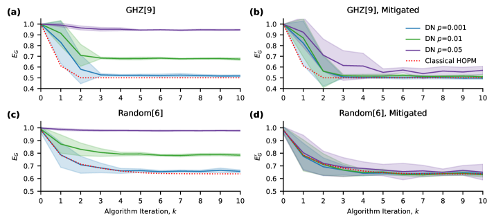
Figure 4: Simulation results for QHOPM on target states GHZ[$9$] and Random[$6$] with the DN model and its mitigation. (a) and (c) show the mean simulation results for QHOPM with input target states GHZ[$9$] and Random[$6$], respectively, for different DN error rates; (b) and (d) show the results of our mitigation procedure (see Eq. (25)) applied to QHOMP simulations on target statesGHZ[$9$] and Random[$6$], respectively. Each simulation was run 10 times (with the same 10 random initial separable states) with $1\times 10^{5}$ shots per each measurement. Solid lines represent the mean geometric entanglement, $E_{G}{}$, and the shaded colours represent the standard deviation. The colour of the lines represents the noise model used for the simulation (see legend). Red dotted lines show results of classical HOPM.

Finally, we apply our migitation technique to results obtained with more realistic noise models. We consider the Qiskit “FakeLima” (representing an older 5 qubit device) and “FakeSherbrooke” (representing a newer device) models that are calibrated to match the error profile of physical devices. To apply our mitigation technique we need to estimate the noise rate $p$ for DN that would approximate the quantum device’s noise. To do this we apply QHOPM to the GHZ state, where the true value of $\widetilde{E}_{G}$ is known. We then use the ratio between the measured $\overline{E}_{G}$ and the true value $\widetilde{E}_{G}$ to estimate $p$ (see Methods, Eq. (26)).

Since GHZ[$9$] is calibrated against itself, to demonstrate our mitigation technique on realistic noise models we show only the state $Random[6]$ ($p$ estimated with GHZ[$6$]). The graph for GHZ[$9$] is in Supplemental Figure 6(f). In Fig. 5(a) we contrast the classical HOPM to FakeLima’s $\overline{E}_{G}\approx 0.685$ with $\sigma_{E_{G}}\approx 0.034$ and FakeSherbrooke’s $\overline{E}_{G}\approx 0.682$ with $\sigma_{E_{G}}\approx 0.028$. For FakeLima we estimated the error rate to be $p\approx 24.68\times 10^{-4}$ and after mitigation we see in Fig. 5(b) that $E_{G}^{\prime}\approx 0.641$; for FakeSherbrooke we estimate the error rate to be $p\approx 25.18\times 10^{-4}$ and compute the mitigated value $E_{G}^{\prime}\approx 0.636$. See Supplementary Materials for more states simulations and mitigation results for these noise models.

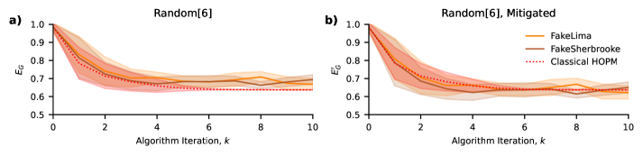
Figure 5: Simulation results of QHOPM for Random[$6$] with more realistic noise models and its mitigation. (a) and (b) show unmitigated and mitigated results for Random[$6$], respectively. Each simulation was run 10 times (with the same 10 random initial separable states) with $1\times 10^{5}$ shots per each measurement. Solid lines represent the mean geometric entanglement, $E_{G}{}$, and the shaded colours represent the standard deviation. The colour of the lines represents the noise model used for the simulation (see legend). Red dotted lines show results of classical HOPM.

3 Discussion

In this work we presented QHOPM, an iterative quantum algorithm for the approximation of the geometric measure of entanglement of pure states on near term quantum devices as well as a noise mitigation technique to improve its experimental resolution. QHOPM is the quantum adaptation of the well-known classical HOPM approach [20, 21, 22, 26, 27, 29] for rank-1 tensor approximation.

While QHOPM does not converge any differently than classical HOPM, its potential utility lies in the observation that it requires only $n+1$ qubits to compute the GE of a quantum state (on $n$ qubits) while an exponential data structure (and so exponential runtime) is assumed by classical HOPM (for quantum states). We also show that the number of measurements required, per algorithm iteration, scales linearly with $n$.

We showed (see Remarks 8 and 9) that the effect of depolarizing noise on QHOPM for the studied noise rates ($p\leq 0.05$) does not affect its convergence, but rather shifts the final result. The same observation was made in simulations using more realistic noise models implemented in IBM Qiskit’s FakeLima and FakeSherbrooke simulation backends. This allowed us to assume and successfully apply the mitigation technique developed for the DN model on these unknown noise channels. The noise rate for the unknown models was estimated using GHZ as a reference state with a known GE.

Another mitigation approach is presented in [46], where the authors assumed that the channel is applied only on the final stage before each measurement with the “total” error rate $p_{tot}$, which they propose to recover from measuring $\operatorname{Tr}(\rho^{2})$. This approach is equivalent to ours if we use $p_{tot}=1-q^{d}$ and treat $p$ and $d$ as parameters (see Remark 9).

Noise analysis was not the main topic of this work and the assumptions we made are simplified. A more consistent and rigorous approach would be to consider application of DN channel to individual gates with different noise rates or to study the noise model of a particular quantum device.

To our knowledge, the only other quantum algorithms for calculating geometric entanglement are variational algorithms where the ansatz is a separable state [32, 31]. We compare one of these, the VDGE algorithm [31], with QHOPM. VDGE converges much more slowly than QHOPM, needing on the order of $10^{2}$ iterations on GHZ compared to QHOPM’s $10^{0}$. The authors of VDGE claim that the optimizer they use (complex simultaneous perturbation stochastic approximation) is robust against noise. It gives results within $\epsilon\approx 10^{-4}$ absolute accuracy for the three qubit random state case, the error gradually grows as the number of qubits increases (e.g.$\epsilon\approx 10^{-2}$ for six qubit random states). We found that on a random 6 qubit state with realistic noise models and a relatively simple mitigation scheme, QHOPM got results within the same range $\epsilon\approx 10^{-2}$. Like QHOPM, these variational approaches are sensitive to the initial separable state and one is never sure if the result obtained is a local minima or the global minimum. Also, like any quantum variational approach, VDGE is prone to have barren plateaus as the number of qubits grow, which makes it hard to implement on large scale devices.

We observe that HOPM may be extended with a shift parameter to a so-called shifted HOPM [47, 27] or Gauss-Seidel method [29]. In the Supplementary Materials we show how we incorporate this change in our algorithm.

An interesting future direction is to extend our method to approximating geometric entanglement of mixed states [19]. For example, the authors of [22] presented a method for approximating GE of a mixed state based on the connection to the so-called revised GE [48] and Uhlmann’s theorem [49]. The classical implementation of the method given in [22] may be naively modified to incorporate techniques presented in the current work for some intermediate steps, but the calculation will still be performed largely on the classical side. Further work is needed to effectively incorporate QHOPM with this method.

Finally, we observe that our algorithm is a quantum application of the alternating least squares (ALS) method applied to the particular system of non-linear equations for estimating rank-1 tensor approximation. The ALS method by itself is an area of interest in classical machine learning [50, 51], perhaps a variant of our approach would be of use in a suitable problem domain.

Methods

3.1 Quantum circuit simulation

We simulate the Hadamard test variant of QHOPM using the Qiskit [45] platform (IBM Qiskit Version 0.46.0). We find in practice that the algorithm gives sufficiently good results when each individual simulation uses $1\times 10^{5}$ shots which corresponds to an absolute accuracy $\epsilon\approx 0.003$.

For a given a target state, regions of initial separable states will converge to different local minima [24]. When using the HOPM algorithm one might try many initial separable states and choose the minimum value obtained. In this work we use 10 random initial states to demonstrate the variation between initial starting points.

To investigate the effect of noise on our algorithm, we use the depolarizing noise (DN) model [49] and more realistic noise models implemented in “FakeLima” and “FakeSherbrooke” backends, developed to mimic real IBM hardware. We let the parameter of the DN model (referred to in this work as “noise rate” or “error rate”) $p\in\{0,0.001,0.01,0.05\}$ and apply DN to all one-, two- and three-qubit gates used in our circuits via the Qiskit AerSimulator.

To demonstrate the performance of QHOPM we chose the following target states:

• 3 qubit W state, with known $E_{G}=5/9$ [19];

• 3, 6, and 9 qubit GHZ states, each with known $E_{G}=0.5$;

• 3, 6 and 9 qubit ring cluster states [3];

• 3, 6 and 9 qubit random states.

To generate Random[$n$] states we created quantum circuits with the following method: we sampled gates (uniformly at random) from the gate set of CNOT and Qiskit’s $U$ gate (general single qubit rotation) with random angles and applied them to uniformly random selected qubits. This process was iterated until the circuit depth reached 10.

The initial random separable states $V^{(0)}$ (see Eq. (5)) were chosen by sampling uniformly at random $\vartheta_{i}\in[0,\pi)$ and $\varphi_{i}\in[0,2\pi)$ for $i=1,\dots,n$.

3.2 Depolarizing noise mitigation

To mitigate the effects of noise on the simulation results we assume the depolarising noise (DN) model [49] in our simulations. The DN channel for a system of $n$ qubits, applied to all the qubits is defined as [49, 52]

$$\mathcal{E}(\rho)=(1-p)\rho+p\frac{1}{2^{n}}I^{n},$$ (14)

where $I$ is a $2$-dimensional identity matrix; $0\leq p\leq 4^{n}/(4^{n}-1)$ is a parameter of the model (which we will refer to as noise rate). When $p=1$ the channel is fully depolarizing. When $p=4^{n}/(4^{n}-1)$ the channel has with (uniformly) random Pauli errors on each qubit.

Typically the DN channel is applied to each gate in a quantum circuit individually and with different rates. This leads to cumbersome analysis and a strong dependence on the structure of the circuit under study. To avoid this here we consider the following simplification: we assume that the DN channel is applied $d$ times at a constant rate $p$ to all qubits after each layer of gates, where $d$ is the circuit depth (maximum number of operations on a qubit in the circuit). The DN channel commutes with any unitary operation:

$$U\,\mathcal{E}(\rho)\,U^{\dagger}=U\left((1-p)\rho+p\frac{I}{2^{n}}\right)U^{\dagger}=\mathcal{E}(U\rho U^{\dagger}),$$

which allows to apply the channel $d$ times at the end of the circuit:

$$\begin{split}\rho=\mathcal{E}^{d}(\rho^{\prime})&=(1-p)^{d}\rho^{\prime}+\frac{p}{2^{n}}\sum_{i=1}^{d}(1-p)^{d-i}I\\ &=q^{d}\rho^{\prime}+\frac{1-q^{d}}{2^{n}}I,\end{split}$$ (15)

where $q=(1-p)$; $\rho^{\prime}$ is a density matrix of a pure state with no noise. The number $d$ is also be understood as the number of times that the DN channel affects the state with the error rate $p$.

Proposition 7.

Having the DN channel defined by Eq. (15) in terms of the Hadamard test procedure, the measured $P_{i}(s)$ and $\lambda^{(k)}$ is expressed as

$$P_{i}(s)\approx\left(1+\eta P_{i}^{\prime}(s^{\perp})+\ldots\right)\,P_{i}^{\prime}(s);$$ (16)

$$\lambda^{(k)}=q^{d}\sqrt{1-\eta\sin^{2}\gamma^{\prime}}\,\lambda^{\prime(k)},$$ (17)

where $\eta=(1-q^{2})$; $P_{i}^{\prime}(s)$, $P_{i}^{\prime}(s^{\perp})$ and $\lambda^{\prime(k)}$ are the noise-free values of $P_{i}(s)$, $P_{i}(s^{\perp})$ and $\lambda^{(k)}$, respectively; dots in Eq. (16) correspond to the terms of the second order and higher in $\eta$; $\gamma^{\prime}$ is the phase of the noise-free scalar product $\bra{\bf 0}{V^{(k)}}^{\dagger}U_{\psi}\ket{\bf 0}=\lambda^{\prime(k)}e^{-i\gamma^{\prime}}$, which is recovered from

$$\tan\gamma^{\prime}=q\frac{\langle Y\rangle_{a}}{\langle X\rangle_{a}}.$$ (18)

Proof.

To obtain $P_{i}(s)$, defined by Eq. (10), we need to measure $u_{i,s}^{(k)}$, which in terms of the Hadamard test procedure is done by measuring

$$\begin{split}&\langle X\rangle_{a}=(P^{(a)}(-)-P^{(a)}(+))=1-2P^{(a)}(+),\\ &\langle Y\rangle_{a}=1-2P^{(a)}(-i),\end{split}$$ (19)

where

$$\begin{split}P^{(a)}(+)=&\operatorname{Tr}(\ket{+}\bra{+}\otimes I^{n-1}\rho)=q^{d}{P^{(a)}}^{\prime}(+)+\frac{1-q^{d}}{2},\\ P^{(a)}(-i)=&\operatorname{Tr}(S^{\dagger}\ket{+}\bra{+}S\otimes I^{n-1}\rho)=q^{d+1}{P^{(a)}}^{\prime}(-i)+\frac{1-q^{d+1}}{2}\end{split}$$ (20)

are the “noisy” probabilities of the ancilla qubit being in the state $\ket{+}$ and $\ket{-i}$, respectively, and ${P^{(a)}}^{\prime}(+)$ and ${P^{(a)}}^{\prime}(-i)$ are their “non-noisy” counterparts. After substituting Eqs. (20) to Eqs. (19), for $u_{i,s}^{(k)}$ we have:

$$|u_{i,s}^{(k)}|^{2}=\langle X\rangle_{a}^{2}+\langle Y\rangle_{a}^{2}=q^{2d}[1-(1-q^{2})\sin^{2}\gamma^{\prime}]|u_{i,s}^{\prime(k)}|^{2},$$ (21)

where $u_{i,s}^{\prime(k)}$ is a non-noisy value of $u_{i,s}^{(k)}$; $\gamma^{\prime}$ is the phase of $u_{i,s}^{\prime(k)}=e^{i\gamma^{\prime}}|u_{i,s}^{\prime(k)}|$, which originates from the global phase and local $z$-rotations. We know (see Remark 3) that in the absence of noise, the global phase does not affect the convergence of the algorithm, however since $d$ for $\langle Y\rangle_{a}^{\prime}=(\lambda^{\prime(k)}\sin\gamma^{\prime})$ is larger, in the noisy case we will have additional terms in the sum in Eq. (21). In the experiment $\gamma^{\prime}$ is recovered from

$$\tan\gamma^{\prime}=\frac{\langle Y\rangle_{a}^{\prime}}{\langle X\rangle_{a}^{\prime}}=q\frac{\langle Y\rangle_{a}}{\langle X\rangle_{a}}.$$

Similarly, we get

$$|u_{i,s^{\perp}}^{(k)}|^{2}=q^{2d+2}[1-(1-q^{2})\sin^{2}\gamma^{\prime}]|u_{i,s^{\perp}}^{\prime(k)}|^{2},$$ (22)

where the angle $\gamma^{\prime}$ is the same as for the state $\ket{s}$, since $U_{s^{\perp}}=U_{s}X$ does not change the phase.

Substituting Eqs. (21) and (22) to Eq. (10), we have for $P_{i}(s)$:

$$P_{i}(s)=\frac{|u^{\prime}_{i,s}|^{2}}{|u^{\prime}_{i,s}|^{2}+|u^{\prime}_{i,s^{\perp}}|^{2}-\eta|u^{\prime}_{i,s^{\perp}}|^{2}}\approx\left(1+\eta P_{i}(s^{\perp})+\ldots\right)P_{i}(s),$$ (23)

where $\eta=(1-q^{2})$; the right-hand side is the Taylor expansion of the left side near $\eta=0$; $P_{i}(s^{\perp})$ is a non-noisy value of $P_{i}(s^{\perp})$. This proves the first statement of the Proposition.

Following the same steps for $\lambda^{(k)}$, assuming that the noise does not affect one-qubit tomography results, we have in terms of the Hadamard test procedure:

$$\begin{split}\lambda^{{(k)}^{2}}&=\langle X\rangle_{a}^{2}+\langle Y\rangle_{a}^{2}=q^{2d}[1-\eta\sin^{2}\gamma^{\prime}]\lambda^{\prime{(k)}^{2}},\end{split}$$ (24)

where $\gamma^{\prime}$ is the argument of non-noisy $\bra{\bf 0}{V^{(k)}}^{\dagger}U_{\psi}\ket{\bf 0}=e^{i\gamma^{\prime}}\lambda^{\prime(k)}$ and is obtained using Eq. (18); $\lambda^{\prime{(k)}}$ is a non-noisy entanglement eigenvalue. This proves the second statement of the Proposition. ∎

Remark 8.

In terms of the Hadamard test procedure, assuming a fixed initial separable state, small noise rates $p\ll 1$ do not affect convergence of QHOPM and contribute mainly to the shift of entanglement eigenvalue, defined by Eq. (17).

Indeed, sufficiently small $p$ will result in $\eta\ll 1$, which allows to neglect the terms with $\eta$ of the first order and higher in Eq. (16) having the main contribution to be the shift in $\lambda$, defined by Eq. (17). The convergence of QHOPM is defined by line 2 in Algorithm 2, where $\lambda^{\prime(k)}$ and $\lambda^{\prime(k-1)}$ change by coefficients different by at most $q=1-p\approx 1$. Putting the accuracy $\epsilon^{\prime}=(q^{d}\epsilon)$ or having a fixed sufficiently large number of iterations allows to avoid the effect of noise on convergence of QHOPM, leaving only the effect of shift in $\lambda$. Note, that this assumes a fixed initial separable state; different initial states might have different convergence.

In this work, the largest error rate we have studied is $p=0.05$ which gives $\eta\approx 0.1$. Thus, according to Proposition 7 and assuming $P_{i}^{\prime}(s)=P_{i}^{\prime}(s^{\perp})=0.5$, $P_{i}(s)$ changes by at most a factor of approximately $1.025$. We neglect this effect in what follows and take into account only the changes of $\lambda^{{(k)}}$, which even for relatively shallow $U_{\psi}$ may have a significant effect. With these assumptions we approximate the true $E_{G}^{\prime}$ as follows:

$$E_{G}^{\prime}=1-\frac{1-E_{G}}{q^{2d}[1-\eta\sin^{2}\gamma^{\prime}]},$$ (25)

where $\gamma^{\prime}$ is obtained from Eq. (18). The denominator of the lower bound $E_{G}^{\prime}\geq 1-\frac{1-E_{G}}{q^{2d+2}}$ is always less (or equal) than one, which means that $E_{G}\geq E_{G}^{\prime}$ within our assumptions, which corresponds to the observed simulation results.

Remark 9.

Proposition 7, Remark 8 and Eq. (25) are valid for a DN channel with the noise rate $p_{tot}=1-q^{d}$ applied once in the end of the circuit just before the measurements.

This is evident from comparing Eq. (14) and Eq. (15), and allows us to conclude that the made simplified assumption, with the appropriate choice of parameters $p$ and $d$, are valid for any noise channel that is approximated by DN model.

3.3 Mitigating error for arbitrary noise models

To mitigate the results of our algorithm on hardware or simulations where the noise model is usually unknown, we use the following procedure. We run the algorithm on a reference state with a known $\widetilde{E}_{G}$ and measure the noisy value $E_{G}$. In our case we chose GHZ[$n$] with $\widetilde{E}_{G}=0.50$ since the value is consistent for any number of qubits. Using this value and Eq. (25) we calculate $p$ as follows:

$$p=1-\left(\frac{1-\widetilde{E}_{G}}{1-\overline{E}_{G}}\right)^{2d}.$$ (26)

The mitigation procedure now proceeds as outlined in the depolarising noise case.

Appendix    Supplementary Materials

A.1 Implementation of Gauss-Seidel method and Shifted HOPM algorithms

The approach presented in this paper allows us to also implement the Gauss-Seidel method (GSM), which (as authors of the work [29] claim) should converge to the global minimum with higher probability. The difference with HOPM is in line 6 of Algorithm 1: it is changed to

$${\mathbf{v}}_{i}^{(k+1)}=\lambda^{(k)}\psi\times_{\hat{i}}\left({\mathbf{v}_{1}^{(k+1)}}^{\ast},\ldots,{\mathbf{v}_{i-1}^{(k+1)}}^{\ast},{\mathbf{v}_{i+1}^{(k)}}^{\ast},\ldots,{\mathbf{v}_{n}^{(k)}}^{\ast}\right)+\beta{\mathbf{v}}_{i}^{(k)},$$ (27)

where $0<\beta\in\mathbb{R}$ is a free parameter of the algorithm.

To implement GSM the only change to our algorithm is in the classical step where we recover the angles $(\tilde{\vartheta}_{i}^{(k+1)},\tilde{\varphi}_{i}^{(k+1)})$ using one-qubit tomography. Instead of Eq. (9) we need to solve the following system of equations to find $({\vartheta}_{i}^{(k+1)},{\varphi}_{i}^{(k+1)})$,

$$A^{2} \cos^{2}\frac{\vartheta_{i}^{(k+1)}}{2}=\left|\lambda^{(k)}e^{-i\tilde{\varphi}_{i}^{(k+1)}/2}\cos\frac{\tilde{\vartheta}_{i}^{(k+1)}}{2}\right.+\left.\beta e^{-i\varphi_{i}^{(k)}/2}\cos\frac{\vartheta_{i}^{(k)}}{2}\right|^{2};$$ (28)

$$A^{2} \sin\vartheta_{i}^{(k+1)}\sin\varphi_{i}^{(k+1)}=(\lambda^{(k)})^{2}\sin\tilde{\vartheta}_{i}^{(k+1)}\sin\tilde{\varphi}_{i}^{(k+1)}+\beta^{2}\sin\vartheta_{i}^{(k)}\sin\varphi_{i}^{(k)}+2\beta\lambda^{(k)}\sin\frac{\tilde{\vartheta}_{i}^{(k+1)}+\vartheta_{i}^{(k)}}{2}\sin\frac{\tilde{\varphi}_{i}^{(k+1)}+\varphi_{i}^{(k)}}{2};$$

$$A^{2} \sin\vartheta_{i}^{(k+1)}\cos\varphi_{i}^{(k+1)}=(\lambda^{(k)})^{2}\sin\tilde{\vartheta}_{i}^{(k+1)}\cos\tilde{\varphi}_{i}^{(k+1)}+\beta^{2}\sin\vartheta_{i}^{(k)}\cos\varphi_{i}^{(k)}+2\beta\lambda^{(k)}\sin\frac{\tilde{\vartheta}_{i}^{(k+1)}+\vartheta_{i}^{(k)}}{2}\cos\frac{\tilde{\varphi}_{i}^{(k+1)}+\varphi_{i}^{(k)}}{2},$$

where

$$A^{2}=(\lambda^{(k)})^{2}+\beta^{2}+2\beta\lambda^{(k)}\cos\frac{\tilde{\vartheta}_{i}^{(k+1)}-\vartheta_{i}^{(k)}}{2}\cos\frac{\tilde{\varphi}_{i}^{(k+1)}-\varphi^{(k)}}{2}$$

is a normalization coefficient.

Note, that GSM is similar to the so-called shifted HOPM (SHOPM) algorithm [47, 27], with the only difference being that SHOPM does not have the current eigenvalue estimate $\lambda^{(k)}$ as a prefactor on the right-hand side of Eq. (27). Thus to get the SHOPM quantum-classical hybrid implementation one needs to set $\lambda^{(k)}$ in Eq. (28) to one.

A.2 Supplemental simulation results

Figure 7: Simulation and mitigation results for the QHOPM algorithm on the W[$3$] state. (a) shows the effect of noise on convergence. (b) shows the effects of mitigation on the noisy simulation. $\widetilde{E}_{G}=5/9\approx 0.554$. Each simulation was run 10 times (with the same 10 random initial separable states) with $1\times 10^{5}$ shots per each measurement. Solid lines represent the mean geometric entanglement, $E_{G}{}$, and the lightly shaded colours represent the standard deviation. The colour of the lines represents the noise model used for the simulation (see legend). Red dotted lines show results of classical HOPM.

Figure 9: Simulation and mitigation results for the QHOPM algorithm on Random states. Row (a) (b) show Random[$3$], (c) (d) show Random[$6$], (e) (f) show Random[$9$]. Column (a) (c) (e) shows the effect of noise on convergence. Column (b) (d) (f) shows the effects of mitigation on the noisy simulation. Each simulation was run 10 times (with the same 10 random initial separable states) with $1\times 10^{5}$ shots per each measurement. Solid lines represent the mean geometric entanglement, $E_{G}{}$, and the lightly shaded colours represent the standard deviation. The colour of the lines represents the noise model used for the simulation (see legend). Red dotted lines show results of classical HOPM.

References

- \bibcommenthead
- [1] Horodecki, R., Horodecki, P., Horodecki, M. & Horodecki, K. Quantum entanglement. Rev. Mod. Phys. 81, 1–94 (2009). URL http://arxiv.org/abs/quant-ph/0702225.
- [2] Wootters, W. K. Quantum entanglement as a quantifiable resource. Philos. Trans. R. Soc. A 356, 1717–1731 (1998). URL https://royalsocietypublishing.org/doi/10.1098/rsta.1998.0244.
- [3] Gühne, O. & Tóth, G. Entanglement detection. Phys. Rep. 474, 1–75 (2009). URL https://www.sciencedirect.com/science/article/pii/S0370157309000623.
- [4] Broadbent, A. & Schaffner, C. Quantum Cryptography Beyond Quantum Key Distribution. Des. Codes Cryptogr. 78, 351–382 (2016). URL http://arxiv.org/abs/1510.06120.
- [5] Vidal, G. Efficient classical simulation of slightly entangled quantum computations. Phys. Rev. Lett. 91, 147902 (2003). URL http://arxiv.org/abs/quant-ph/0301063. ArXiv:quant-ph/0301063.
- [6] Gottesman, D. Theory of fault-tolerant quantum computation. Phys. Rev. A 57, 127–137 (1998). URL https://link.aps.org/doi/10.1103/PhysRevA.57.127.
- [7] Gottesman, D. The Heisenberg Representation of Quantum Computers. Group22: Proceedings of the XXII International Colloquium on Group Theoretical Methods in Physics (1998). URL http://arxiv.org/abs/quant-ph/9807006.
- [8] Aaronson, S. & Gottesman, D. Improved simulation of stabilizer circuits. Phys. Rev. A 70, 052328 (2004). URL https://link.aps.org/doi/10.1103/PhysRevA.70.052328.
- [9] Gross, D., Flammia, S. T. & Eisert, J. Most quantum states are too entangled to be useful as computational resources. Phys. Rev. Lett. 102, 190501 (2009). URL https://link.aps.org/doi/10.1103/PhysRevLett.102.190501.
- [10] Patti, T. L., Najafi, K., Gao, X. & Yelin, S. F. Entanglement devised barren plateau mitigation. Phys. Rev. Research 3, 1–10 (2021). URL https://link.aps.org/doi/10.1103/PhysRevResearch.3.033090.
- [11] Marrero, C. O., Kieferová, M. & Wiebe, N. Entanglement Induced Barren Plateaus. PRX Quantum 2, 1–14 (2021). URL http://arxiv.org/abs/2010.15968.
- [12] Georgiev, D. D. & Gudder, S. P. Sensitivity of entanglement measures in bipartite pure quantum states. Mod. Phys. Lett. B 36, 1–26 (2022).
- [13] Wootters, W. K. Entanglement of formation of an arbitrary state of two qubits. Phys. Rev. Lett. 80, 2245–2248 (1998). URL https://link.aps.org/doi/10.1103/PhysRevLett.80.2245.
- [14] Love, P. J. et al. A Characterization of Global Entanglement. Quantum Inf. Process. 6, 187–195 (2007). URL https://doi.org/10.1007/s11128-007-0052-7.
- [15] Plbnio, M. B. & Virmani, S. An introduction to entanglement measures. Quantum Info. Comput. 7, 1–51 (2007).
- [16] Dür, W., Vidal, G. & Cirac, J. I. Three qubits can be entangled in two inequivalent ways. Phys. Rev. A 62, 1–11 (2000). URL https://link.aps.org/doi/10.1103/PhysRevA.62.062314.
- [17] Shimony, A. Degree of Entanglement. Ann. N.Y. Acad. Sci. 755, 675–679 (1995). URL https://onlinelibrary.wiley.com/doi/abs/10.1111/j.1749-6632.1995.tb39008.x.
- [18] Barnum, H. & Linden, N. Monotones and invariants for multi-particle quantum states. J. Phys. A: Math. Gen. 34, 1–12 (2001). URL https://dx.doi.org/10.1088/0305-4470/34/35/305.
- [19] Wei, T.-C. & Goldbart, P. M. Geometric measure of entanglement and applications to bipartite and multipartite quantum states. Phys. Rev. A 68, 1–12 (2003). URL https://link.aps.org/doi/10.1103/PhysRevA.68.042307.
- [20] Shimoni, Y., Shapira, D. & Biham, O. Entangled quantum states generated by Shor’s factoring algorithm. Phys. Rev. A 72, 062308 (2005). URL https://link.aps.org/doi/10.1103/PhysRevA.72.062308.
- [21] Most, Y., Shimoni, Y. & Biham, O. Entanglement of periodic states, the quantum fourier transform, and shor’s factoring algorithm. Phys. Rev. A 81, 052306 (2010). URL https://link.aps.org/doi/10.1103/PhysRevA.81.052306.
- [22] Streltsov, A., Kampermann, H. & Bruß, D. Simple algorithm for computing the geometric measure of entanglement. Phys. Rev. A 84, 022323 (2011). URL https://link.aps.org/doi/10.1103/PhysRevA.84.022323.
- [23] Teng, P. Accurate calculation of the geometric measure of entanglement for multipartite quantum states. Quantum Inf. Process. 16, 1–17 (2017). URL http://arxiv.org/abs/1609.02076.
- [24] De Lathauwer, L., De Moor, B. & Vandewalle, J. On the best rank-1 and rank-( , ,,) approximation of higher-order tensors. SIAM J. Matrix Anal. Appl. 21, 1324–1342 (2000). URL https://doi.org/10.1137/S0895479898346995.
- [25] Hayashi, M., Markham, D., Murao, M., Owari, M. & Virmani, S. The geometric measure of entanglement for a symmetric pure state with non-negative amplitudes. J. Math. Phys. 50, 122104 (2009). URL https://doi.org/10.1063/1.3271041.
- [26] Ni, G., Qi, L. & Bai, M. Geometric Measure of Entanglement and U-Eigenvalues of Tensors. SIAM J. Matrix Anal. Appl. 35, 73–87 (2014). URL https://epubs.siam.org/doi/abs/10.1137/120892891.
- [27] Hu, S., Qi, L. & Zhang, G. Computing the geometric measure of entanglement of multipartite pure states by means of non-negative tensors. Phys. Rev. A 93, 012304 (2016). URL https://link.aps.org/doi/10.1103/PhysRevA.93.012304.
- [28] Qi, L., Zhang, G. & Ni, G. How entangled can a multi-party system possibly be? Phys. Lett. A 382, 1465–1471 (2018). URL https://www.sciencedirect.com/science/article/pii/S0375960118303621.
- [29] Zhang, M., Ni, G. & Zhang, G. Iterative methods for computing U-eigenvalues of non-symmetric complex tensors with application in quantum entanglement. Comput. Optim. Appl. 75, 779–798 (2020). URL https://doi.org/10.1007/s10589-019-00126-5.
- [30] Chatelin, F. Eigenvalues of Matrices (Society for Industrial and Applied Mathematics, 2012).
- [31] Muñoz Moller, A., Pereira, L., Zambrano, L., Cortés-Vega, J. & Delgado, A. Variational determination of multiqubit geometrical entanglement in noisy intermediate-scale quantum computers. Phys. Rev. Applied 18, 1–7 (2022). URL https://link.aps.org/doi/10.1103/PhysRevApplied.18.024048.
- [32] Consiglio, M., Apollaro, T. J. G. & Wieśniak, M. Variational approach to the quantum separability problem. Phys. Rev. A 106, 1–12 (2022). URL https://link.aps.org/doi/10.1103/PhysRevA.106.062413.
- [33] Bernardi, A., Carlini, E., Catalisano, M. V., Gimigliano, A. & Oneto, A. The hitchhiker guide to: Secant varieties and tensor decomposition. Mathematics 6 (2018). URL https://www.mdpi.com/2227-7390/6/12/314.
- [34] Cirici, J., Salvadó, J. & Taron, J. Characterization of quantum entanglement via a hypercube of segre embeddings. Quantum Inf. Process. 20, 1–23 (2021). URL https://link.springer.com/article/10.1007/s11128-021-03186-x.
- [35] Ballico, E., Bernardi, A., Carusotto, I., Mazzucchi, S. & Moretti, V. Quantum Physics and Geometry (Springer Cham, 2019).
- [36] Draisma, J., Horobeţ, E., Ottaviani, G., Sturmfels, B. & Thomas, R. R. The euclidean distance degree of an algebraic variety. Found. Comput. Math. 16, 99–149 (2016). URL https://link.springer.com/article/10.1007/s10208-014-9240-x.
- [37] Hillar, C. J. & Lim, L.-H. Most tensor problems are NP-hard. J. ACM 60 (2013). URL https://doi.org/10.1145/2512329.
- [38] Chen, L., Han, L. & Zhou, L. Computing tensor eigenvalues via homotopy methods. SIAM J. Matrix Anal. Appl. 37, 290–319 (2016). URL https://doi.org/10.1137/15M1010725.
- [39] Lieven De Lathauwer, B. D. M. & Vandewalle, J. A multilinear singular value decomposition. SIAM J. Matrix Anal. Appl. 21, 1253–1278 (2000). URL https://doi.org/10.1137/S0895479896305696.
- [40] Kroonenberg, P. M. & de Leeuw, J. Principal component analysis of three-mode data by means of alternating least squares algorithms. Psychometrika 45, 69–97 (1980). URL https://doi.org/10.1007/BF02293599.
- [41] Cleve, R., Ekert, A., Macchiavello, C. & Mosca, M. Quantum algorithms revisited. Proc. R. Soc. London, Ser. A. 454, 339–354 (1998). URL https://royalsocietypublishing.org/doi/10.1098/rspa.1998.0164.
- [42] Regalia, P. & Kofidis, E. The higher-order power method revisited: convergence proofs and effective initialization. Proceedings of the Acoustics, Speech, and Signal Processing 5, 2709–2712 (2000). URL https://ieeexplore.ieee.org/document/861047.
- [43] Uschmajew, A. A new convergence proof for the higher-order power method and generalizations. Pac. J. Optim. 11, 309–321 (2015). URL http://manu71.magtech.com.cn/Jwk3_pjo/EN/Y2015/V11/I2/309#3.
- [44] Hu, S. & Li, G. Convergence rate analysis for the higher order power method in best rank one approximations of tensors. Numer. Math. 140, 993–1031 (2018).
- [45] Qiskit contributors. Qiskit: An open-source framework for quantum computing (2023).
- [46] Vovrosh, J. et al. Simple mitigation of global depolarizing errors in quantum simulations. Phys. Rev. E 104, 035309 (2021). URL https://link.aps.org/doi/10.1103/PhysRevE.104.035309.
- [47] Kolda, T. G. & Mayo, J. R. Shifted power method for computing tensor eigenpairs. SIAM Journal on Matrix Analysis and Applications 32, 1095–1124 (2011). URL https://doi.org/10.1137/100801482.
- [48] Streltsov, A., Kampermann, H. & Bruß, D. Linking a distance measure of entanglement to its convex roof. New J. Phys. 12, 2–18 (2010). URL https://dx.doi.org/10.1088/1367-2630/12/12/123004.
- [49] Nielsen, M. A. & Chuang, I. L. Quantum Computation and Quantum Information (Cambridge University Press, 2010).
- [50] Zhou, Y., Wilkinson, D., Schreiber, R. & Pan, R. Fleischer, R. & Xu, J. (eds) Large-Scale Parallel Collaborative Filtering for the Netflix Prize. (eds Fleischer, R. & Xu, J.) Algorithmic Aspects in Information and Management, 337–348 (Springer, Berlin, Heidelberg, 2008).
- [51] Xu, Z. & Li, P. Wallach, H. et al. (eds) Towards practical alternating least-squares for CCA. (eds Wallach, H. et al.) Advances in Neural Information Processing Systems, Vol. 32 (Curran Associates, Inc., 2019). URL https://proceedings.neurips.cc/paper_files/paper/2019/file/af3b6a54e9e9338abc54258e3406e485-Paper.pdf.
- [52] Emerson, J., Alicki, R. & Zyczkowski, K. Scalable noise estimation with random unitary operators. J. Opt. B: Quantum Semiclass. Opt 7, S347–S352 (2005).