Apparent horizon tracking in supercritical solutions of the Einstein-scalar field equations in spherical symmetry in affine-null coordinates

Abstract

Choptuik’s critical phenomena in general relativity is revisited in the affine-null metric formulation of Einstein’s equations for a massless scalar field in spherical symmetry. Numerical solutions are obtained by evolution of initial data using pseudo-spectral methods. The underlying system consists of differential equations along the outgoing null rays which can be solved in sequential form. A new two-parameter family of initial data is presented for which these equations can be integrated analytically. Specific choices of the initial data parameters correspond to either an asymptotically flat null cone, a black hole event horizon or the singular interior of a black hole. Our main focus is on the interior features of a black hole, for which the affine-null system is especially well adapted. We present both analytic and numerical results describing the geometric properties of the apparent horizon and final singularity. Using a re-gridding technique for the affine parameter, numerical evolution of initially asymptotically flat supercritical data can be continued inside the event horizon and track the apparent horizon up to the formation of the final singularity.

I Introduction

Choptuik’s Choptuik:1993PRL discovery of critical phenomena in general relativity is one of the first major results of the numerical investigation of the Einstein equations. At its heart is the discretely self-similar (DSS) critical solution of the Einstein equations for a spherical symmetric massless-scalar field which evolves to form a naked singularity with zero mass. The scalar field is periodic with respect to a time scale adapted to the discrete conformal symmetry, with twice the period $\Delta\approx 3.44$ of the corresponding conformal metric Choptuik:1993PRL ; 1995PhRvL..75.3214G ; 1997PhRvD..55.3485H ; 1996CQGra..13..497H . Until recently, the existence of the critical solution and its properties have only been inferred by numerical evolution. However, the existence of this critical DSS solution has been established and its properties studied by purely analytic methods 2019CMaPh.368..143R . By calculating the inverse of an elliptic operator, the authors of 2019CMaPh.368..143R provide a value for $\Delta$ with an accuracy of $10^{-80}$.

Choptuik observed that a one parameter family of asymptotically flat initial data, with parameter $p$, evolves to either a flat space-time or to a black hole, with the two alternatives intermediated by a critical value $p^{*}$. Here $p<p^{*}$ for subcritical (weak) initial data and $p>p^{*}$, for supercritical (strong) initial data. For supercritical evolution, he found that the mass $m$ of the black hole obeys a universal scaling relation $m\sim|p-p^{*}|^{\gamma}$, with $\gamma\approx 0.37$, independent of the particular form of the initial data. Further analysis revealed a modified scaling law $\ln(m)=\gamma\ln|p^{*}-p|+F\left[\frac{2\pi}{\Delta}(p^{*}-p)\right]$, where $F$ is a periodic function of $\Delta$ 1995PhRvL..75.3214G ; 1996CQGra..13..497H ; 1997PhRvD..55.3485H ; 1997PhRvD..55..695G ; 1995PhRvD..51.4198H (See 2007LRR….10….5G for a review.)

For the critical case $p=p^{*}$, there is a value $\tau=\tau^{*}$ of the proper time along the central geodesic for formation of the final singularity, with $\tau^{*}$ dependent upon the particular initial data. For supercritical initial data, the evolution leads to a black hole for $\tau>\tau^{*}$. Several studies, e.g. 1997PhRvD..55.3485H ; 1996CQGra..13..497H ; 2003PhRvD..68b4011M , indicate that the echoing period $\Delta$ is adapted to the “logarithmic time” coordinate $\xi=-\log(\tau^{*}-\tau)$, i.e. the metric satisfies $e^{-2\Delta}g_{ab}(\xi+\Delta)=g_{ab}(\xi)$ and the scalar field satisfies $\Phi(\xi+\Delta)=-\Phi(\xi)$.

Because the echoing occurs with respect to the logarithmic time $\xi$, its resolution in terms of the proper time $\tau$ is numerically challenging. Higher and higher resolution is required when $\tau\lesssim\tau^{*}$ and the time $\Delta\tau$ between subsequent periods decreases exponentially. This has been referred to as the “loss of grid points” near the central worldline close to formation of the critical solution Garfinkle:1994jb ; Purrer:2004nq .

In this work, we extend the investigation CW2019 of critical collapse in affine null coordinates $(u,\lambda,x^{A})$, where $u$ measures the proper time along the central timelike geodesic and $\lambda$ is an affine parameter along the spherical congruence of outgoing null rays, which are labeled by angular coordinates $x^{A}$. We present the underlying formalism in Sec. II. We modify the evolution algorithm in CW2019 to allow tracking of the apparent horizon and introduce a novel two-parameter set of initial data for which the null hypersurface equations can be integrated analytically. Specific choices of the initial data parameters correspond to either an asymptotically flat null cone, a black hole event horizon or the singular interior of a black hole.

As opposed to the numerical investigation of the Choptuik problem in 2002PhRvD..65h1501L ; Purrer:2004nq using Bondi null coordinates based upon a surface area radius $r$, the affine null system allows evolution inside the event horizon where the $r$ coordinate is singular at the apparent horizon. Thus evolution inside the event horizon breaks down in Bondi coordinates (see Win2013 for further discussion). For the choice of black hole initial data, the affinely parametrized null cones extend smoothly across the apparent horizon, where the expansion of the outgoing null cones vanishes, and up to the final singularity, where the null cones re-converge to a point. This allows a combination of analytic and numerical methods to investigate the interior of the black hole.

In comparsion with CW2019 , we use a single domain spectral method based on the standard Chebysheff polynomials, combined with the grid compactification of null infinity described in 2012LRR….15….2W and used in several other characteristic codes 2015CQGra..32b5008H ; 2016CQGra..33v5007H . Accuracy near the central worldline is increased by filling a local set of collocation points with values obtained from a Taylor series about the origin. Further details of the numerical techniques are given in Sec. V.

By a combination of analytic and numerical results, we are able to establish for the case of supercritical initial data that the apparent horizon and final singularity are both spacelike hypersurfaces. These results are schematically represented for the compactified spacetime in Fig. 1

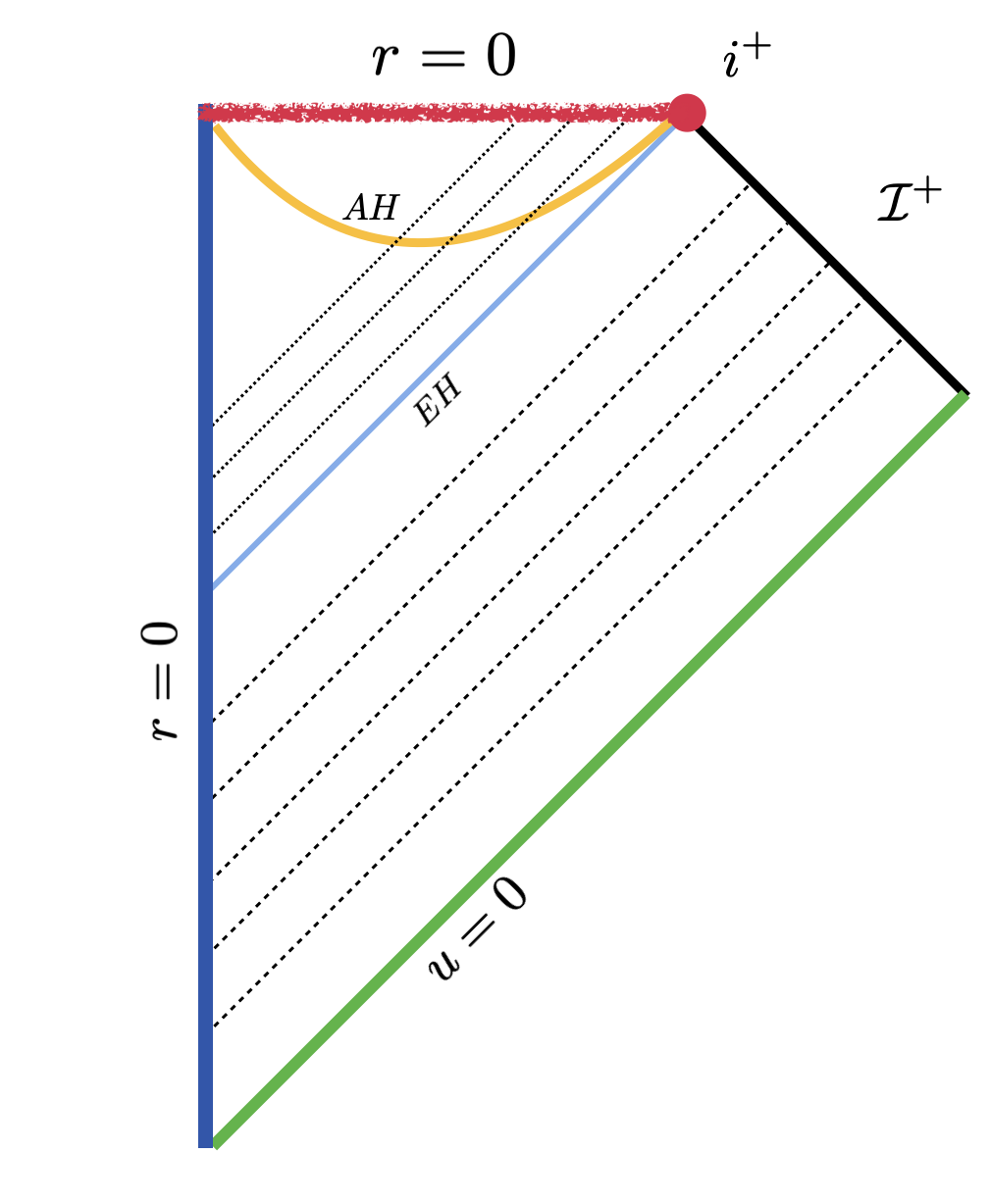
Figure 1: Conformal diagram of a supercritical evolution. The outgoing null hypersurface $u=0$ is the initial data surface extending to null infinity ${\cal I}^{+}$. $EH$ is the future event horizon $H^{+}$ which extends to timelike infinity $i^{+}$.The hypersurface $AH$ is the apparent horizon. The outgoing null cones re-converge to the final singularity at $r=0$

We use geometric units in which $c=8\pi G=1$ . Covariant derivatives are denoted by $\nabla$ and partial derivatives are often used in comma notation, i.e. $\partial f/\partial x^{a}=f_{,a}$.

II Affine null-metric formalism for the Einstein-scalar field equations in spherical symmetry

The spherically symmetric metric in affine-null coordinates $u,\lambda,x^{A}$ is given by Win2013 ; TM2019 ; CW2019 ; 2023PhRvD.107j4010M ; 2021PhRvD.104h4048G

$$ds^{2}=-V(u,\lambda)du^{2}-2dud\lambda+r^{2}(u,\lambda)q_{AB}(x^{C})dx^{A}dx^{B},$$ (1)

where the outgoing null cones are labeled by the proper time $u$ along the central worldline, $\lambda$ is an affine parameter along the spherical congruence of outgoing null rays, which are labeled by angular coordinates $x^{A}$. Here $q_{AB}$ is the unit sphere metric.

We require regularity along the central wordline, where we use the affine freedom $\lambda\rightarrow A\lambda+B$ to set $\lambda=0$ and $r_{,\lambda}=1$ on the central worldline. This gives rise to the local Minkowski coordinate conditions

$$r(u,0)=0\;,\;r_{,\lambda}(u,0)=1\;,\;V(u,0)=1\;,\;V_{,\lambda}(u,0)=0.$$ (2)

(For discussion of these coordinate conditions for the Bondi-Sachs formalism see e.g. TM2013 ).

The Einstein equations for a massless scalar field $\Phi$ are given in terms of the Ricci tensor $R_{ab}$ by

$$E_{ab}:=R_{ab}-\Phi_{,a}\Phi_{,b}=0,$$ (3)

with components

$$E_{uu}:\;\; 0=-\frac{2}{r}r_{,uu}+\frac{V}{2r^{2}}(r^{2}V_{,\lambda})_{,\lambda}+\frac{r_{,\lambda}V_{,u}}{r}$$

$$\qquad-\frac{r_{,u}V_{,\lambda}}{r}-\Phi_{,u}^{2}$$ (4a)

$$E_{u\lambda}:\;\; 0=\frac{1}{2r^{2}}(r^{2}V_{,\lambda})_{,\lambda}-\frac{2r_{,u\lambda}}{r}-\Phi_{,u}\Phi_{,\lambda}$$ (4b)

$$E_{\lambda\lambda}:\;\; 0=-\frac{2}{r}r_{,\lambda\lambda}-(\Phi_{,\lambda})^{2}$$ (4c)

$$q^{AB}E_{AB}:\;\; 0=-[V(r^{2})_{,\lambda}-2\lambda-2(r^{2})_{,u}]_{,\lambda}$$ (4d)

and the wave equation $\nabla_{a}\nabla^{a}\Phi=0$, which takes the form

$$0=(r^{2}\Phi_{,u})_{,\lambda}+(r^{2}\Phi_{,\lambda})_{,u}-(r^{2}V\Phi_{,\lambda})_{,\lambda}\;\;.$$ (5)

Equations (4) have a scale symmetry: If $\Phi(u,\lambda)$, $V(u,\lambda)$, $r(u,\lambda)$ is a solution then so is ${\hat{\Phi}(u,\lambda)=\Phi(\hat{u},\hat{\lambda})}$, ${\hat{V}(u,\lambda)=V(\hat{u},\hat{\lambda})}$ and ${\hat{r}(u,\lambda)=\alpha^{-1}r(\hat{u},\hat{\lambda})}$, where $(\hat{u},\hat{\lambda})=(\alpha u,\alpha\lambda)$.

If $E_{\lambda\lambda}$, $q^{AB}E_{AB}$ and $\nabla_{a}\nabla^{a}\Phi=0$ hold everywhere, then the Bianchi identities imply that (i) $E_{u\lambda}$ holds trivially and (ii)

$$0=(r^{2}E_{uu})_{,\lambda}$$ (6)

so that if $r^{2}E_{uu}$ holds for one value $\lambda$, it holds everywhere. Therefore, since regularity requires $r^{2}E_{uu}$ to vanish at the central word line where $r=0$, we need only enforce the three main equations $E_{\lambda\lambda}$, $q^{AB}E_{AB}$ and $\nabla_{a}\nabla^{a}\Phi=0$ in a numerical simulation.

The Einstein equation (4d) can readily be integrated to find

$$V=\frac{C(u)+2\lambda+2(r^{2})_{,u}}{(r^{2})_{,\lambda}},$$ (7)

where the coordinate conditions (2) require that the constant $C=0)$. Consequently,

$$V=\frac{\lambda}{rr_{,\lambda}}+2\frac{r_{,u}}{r_{,\lambda}}.$$ (8)

For future reference, the Ricci scalar, $\mathcal{R}=g^{ab}R_{ab}$ is given by

$$\begin{split}r^{2}\mathcal{R}=&4r_{,\lambda}r_{,u}+8rr_{,u\lambda}-4r\left(r_{,\lambda}V\right)_{,\lambda}\\ &-2(r_{,\lambda})^{2}V-r^{2}V_{,\lambda\lambda}+2,\end{split}$$ (9)

which according to (8) reduces to

$$\mathcal{R}=\frac{2\lambda r_{,\lambda}}{r^{3}}-V_{,\lambda\lambda}-\frac{2}{r^{2}}.$$ (10)

Using (8), the line element for the affine null metric with regular origin becomes

$$ds^{2}=-\Big{(}\frac{\lambda+2rr_{,u}}{rr_{,\lambda}}\Big{)}du^{2}-2d\lambda du+r^{2}q_{AB}dx^{A}dx^{B},$$ (11)

which shows that the metric is entirely determined once $r$ is known. Given regular initial data $r=r(u_{0},\lambda)$ on the null hypersurface $u=u_{0}$, integration of (4c) then determines the initial value of the scalar field according to

$$\Phi(u_{0},\lambda)=\int_{0}^{\lambda}d\tilde{\lambda}\sqrt{-\frac{2r_{,\tilde{\lambda}\tilde{\lambda}}(u_{0},\tilde{\lambda})}{r(u_{0},\tilde{\lambda})}}\;\;.$$ (12)

We use this procedure for construction of initial data in Sec. III.

II.1 Some general physical properties

In spherical symmetry the Misner-Sharp mass

$$m=\frac{r}{2}(1-g^{ab}r_{,a}r_{,b})=\frac{1}{2}(r-\lambda r_{,\lambda})$$ (13)

provides an invariant quasi-local definition of mass, which is related to the Bondi mass $M_{B}$ of an asymptotically flat null cone by

$$M_{B}=\lim_{\lambda\rightarrow\infty}m.$$ (14)

Asymptotic flatness also implies

$$\Phi(u,\lambda)=\frac{\Phi_{[1]}(u)}{\lambda}+\frac{\Phi_{[2]}(u)}{\lambda^{2}}+\mathcal{O}(\lambda^{3})$$ (15)

where the gauge freedom $\Phi\rightarrow\Phi+const$ is used to set $\Phi(u,\lambda)\rightarrow 0$ as $\lambda\rightarrow\infty$. Then (4c) implies

$$r(u,\lambda)=H(u)\lambda+2M_{B}(u)+\mathcal{O}(\lambda^{-1})$$ (16)

where $H=\lim_{\lambda\rightarrow\infty}r_{,\lambda}$ is a function of integration. The Bondi time $u_{B}$ for an inertial observer at infinity is related to the proper time $u$ at the origin by

$$u_{B,u}=\frac{1}{H}\;.$$ (17)

For $H<1$, the Bondi time for an observer at infinity runs faster and it takes an infinite Bondi time to reach the event horizon but only a finite central time. Consequently, an infinite observer is red shifted with respect to a freely falling observer at the origin. An event horizon forms at a time $u_{E}$ when

$$\lim_{u\rightarrow u_{E}}H=0,$$ (18)

i.e. when the redshift becomes infinite and a black hole forms. Thus $H$ monitors the communication between an observer at the central world and an inertial observer at null infinity. When $H=0$ such communication is not possible and the central world line enters an event horizon. At that time (16) shows that $\lim_{u\rightarrow u_{E},\lambda\rightarrow\infty}r_{,\lambda}=0$. Here $r_{,\lambda}$ is related to the expansion $\Theta^{+}$ of the outgoing null cones by

$$\Theta^{+}=\frac{2r_{,\lambda}}{r}.$$ (19)

Upon further evolution, when the central worldline enters the black hole, the null cones form an apparent horizon where $r_{,\lambda}(u,\lambda_{A})=0$ and the expansion vanishes at a finite affine value $\lambda_{A}$. Indeed, (4c) shows that $r_{,\lambda}$ is a monotonically decreasing function of $\lambda$ so that the expansion becomes negative and the $\lambda_{A}(u)$ 2-spheres are trapped for $\lambda>\lambda_{A}$. The outgoing null cones then re-converge to a point caustic at some finite affine value $\lambda_{C}>\lambda_{A}$, located at the final singularity, where $\Theta^{+}\rightarrow-\infty$.

According to (13), the mass of the apparent horizon is given by ${m(u)=r(u,\lambda_{A})/2}$. Also, the regularity of the metric component $g_{uu}$ at the apparent horizon implies, via (8), that

$$\lambda_{A}(u)=-2r(u,\lambda_{A})r_{,u}(u,\lambda_{A}).$$ (20)

The normal vector to the apparent horizon $r_{,\lambda}(u,\lambda_{A})=0$ has norm

$$g^{ab}\nabla_{a}r_{,\lambda}\nabla_{b}r_{,\lambda}|_{\lambda=\lambda_{A}}=r_{,\lambda\lambda}(Vr_{,\lambda\lambda}-2r_{,\lambda u})|_{\lambda=\lambda_{A}}.$$ (21)

But (8) implies

$$rr_{,\lambda}V=\lambda+2rr_{,u}$$ (22)

so that

$$rr_{,\lambda\lambda}V\bigg{|}_{\lambda_{A}}=1+2rr_{,\lambda u}\bigg{|}_{\lambda_{A}}.$$ (23)

Thus the norm is given by

$$g^{ab}\nabla_{a}r_{,\lambda}\nabla_{b}r_{,\lambda}\bigg{|}_{\lambda_{A}}=\frac{r_{,\lambda\lambda}}{r}\bigg{|}_{\lambda_{A}}=-\frac{\Phi_{,\lambda}^{2}}{2}\bigg{|}_{\lambda_{A}}<0$$ (24)

so that the apparent horizon is a spacelike hypersurface, as expected from the general theory.

The numerical algorithm is designed to evolve in a timelike direction, which requires that the metric variable $V>0$. Thus the sign of $V$ is important. In Sec. II.3 we show that $V>0$ in the region where $r>\lambda$ (see (40)). Near the origin, $r\approx\lambda$ and $r_{,\lambda}\approx 1$. Furthermore, throughout a region containing the apparent horizon, where $r$ attains its maximum value, $r$ is a monotonically increasing function of $\lambda$. Thus $r>\lambda$ and $V>0$ throughout the exterior asymptotically flat region and in a region inside the event horizon $0\leq\lambda<\lambda_{A}<\lambda_{V}$, which contains the apparent horizon.

At the apparent horizon, (23) implies

$$1+2rr_{,\lambda u}\bigg{|}_{\lambda_{A}}<0.$$ (25)

The value $\lambda_{V}$ where $V=0$ satisfies

$$(\lambda+2rr_{,u})|_{\lambda_{V}}=0\;\;.$$ (26)

Thus $\lambda+2rr_{,u}$ must have a maximum between $\lambda_{A}$ and $\lambda_{V}$. On the assumption that the gradient $r_{,a}$ remains finite at the final singularity as $r\rightarrow 0$, (8) implies $V\rightarrow\lambda/(rr_{,\lambda})\rightarrow-\infty$ as $\lambda\rightarrow\lambda_{C}$, so that the $u$-direction eventually becomes spacelike. This issue is discussed further in Sec. III.1.

The norm of the $r=const$ hypersurfaces is given by

$$g^{ab}\nabla_{a}r\nabla_{b}r=Vr_{,\lambda}r_{,\lambda}-2r_{,\lambda}r_{,u}=\frac{\lambda r_{,\lambda}}{2r}.$$ (27)

Since $r_{,\lambda}$ is a monotonically decreasing function of $\lambda$ these hypersurfaces are timelike inside the apparent horizon, null at the apparent horizon and spacelike past the apparent horizon. In particular, the final singularity at $\lambda=\lambda_{C}$ is spacelike.

II.2 Main equations as a hierarchy

Because of the appearance of $r_{,u}$ in (4d), the main equations (4c), (4d) and (5) do not have the hierarchical structure of the Bondi-Sachs equations which can be integrated in sequential order BMS ; TW1966 ; Maedler:2016 . A method to restore a hierarchy was presented in CW2019 . Introduction of the term

$$K:=2r_{,\lambda}\Phi_{,u}-2r_{,u}\Phi_{,\lambda}$$ (28)

allows the wave equation (5) to be written as the null hypersurface equation

$$r\Big{(}\frac{rK}{r_{,\lambda}}\Big{)}_{,\lambda}=\left(\frac{r\lambda\Phi_{,\lambda}}{r_{,\lambda}}\right)_{,\lambda}\;.$$ (29)

The $u$-derivative of $\Phi$ is then determined from $K$,

$$\Phi_{,u}=\frac{K}{2r_{,\lambda}}+\frac{r_{,u}}{r_{,\lambda}}\Phi_{,\lambda}\;\;.$$ (30)

Next, the hypersurface equation for $r_{,u}$ results from the $u$-derivative of (4c). This leads to three ordinary differential equations for $r,\;K$ and $r_{,u}$,

$$r_{,\lambda\lambda}= -\frac{r}{2}\Phi_{,\lambda}^{2}$$ (31a)

$$\Big{(}\frac{rK}{r_{,\lambda}}\Big{)}_{,\lambda}= \frac{1}{r}\Big{(}\frac{r\lambda\Phi_{,\lambda}}{r_{,\lambda}}\Big{)}_{,\lambda}$$ (31b)

$$\Big{(}\frac{r_{,u}}{r_{,\lambda}}\Big{)}_{,\lambda\lambda}= -\frac{r\Phi_{,\lambda}}{2r_{,\lambda}}\Big{(}\frac{K}{r_{,\lambda}}\Big{)}_{,\lambda},$$ (31c)

which can be integrated in sequential order, with $\Phi_{,u}$ then determined from (30).

II.3 Regularized version of the equations

In the exterior asymptotically flat region, where $r_{,\lambda}\neq 0$, (31) and (30) provides a well defined evolution algorithm. However, for evolution inside a black hole, a regularization scheme is necessary to remove singular $1/r_{,\lambda}$ terms in (31). Such terms are not due to coordinate singularities but seem to be an artifact of the affine-null equations. Here we present a brief account of the regularization procedure in CW2019 .

Introduction of the variable

$$L= \frac{rK-\lambda\Phi_{,\lambda}}{r_{,\lambda}}=2r\Phi_{,u}-rV\Phi_{,\lambda}$$ (32)

allows us replace (31b) by

$$L_{,\lambda}=\frac{\lambda}{r}\Phi_{,\lambda}\,,$$ (33)

which can be integrated from $\lambda=0$ using the regularity condition $L(u,0)=0$ at the origin. Here the Ricci scalar (10) has a simple expression in terms of the new variable,

$$\mathcal{R}=-\frac{L\Phi_{,\lambda}}{r}.$$ (34)

For the regularisation of (31c), we introduce the variable

$$Q=\frac{V-1}{\lambda}=\frac{2rr_{,u}+\lambda-rr_{,\lambda}}{\lambda rr_{,\lambda}}\,,$$ (35)

which satisfies

$$Q_{,\lambda}=\frac{1}{\lambda^{2}}-\frac{1}{r^{2}}+\frac{1}{2}\left(\frac{L}{\lambda}\right)^{2}.$$ (36)

This equation can be integrated from $\lambda=0$ using the regularity condition $Q(u,0)=0$. Note that the right hand side of (36) contains the terms $1/\lambda^{2}$ and $1/r^{2}$ which are singular at the origin but combine to form a regular function. This is handled by numerical techniques in Sec. V.

In summary, the hierarchical evolution system (31) takes the regularized form

$$r_{,\lambda\lambda}= -\frac{r}{2}\Phi_{,\lambda}^{2}$$ (37a)

$$L_{,\lambda}= \frac{\lambda}{r}\Phi_{,\lambda}$$ (37b)

$$Q_{,\lambda}= \frac{1}{\lambda^{2}}-\frac{1}{r^{2}}+\frac{1}{2}\left(\frac{L}{\lambda}\right)^{2}$$ (37c)

$$\Phi_{,u}= \frac{1+\lambda Q}{2}\Phi_{,\lambda}+\frac{L}{2r}.$$ (37d)

The right hand sides of these equations remain regular up to the formation of the final singularity at $\lambda=\lambda_{C}$, where $r=0$. However, numerical treatmen of the right hand side of (37c) requires special attention near the origin, where cancellations lead to

$$Q_{,\lambda}(u,\lambda)=\frac{2}{3}\Phi_{,\lambda}^{2}(u,0)+\mathcal{O}(\lambda)\;.$$ (38)

Given initial data $\Phi(u_{0},\lambda)$ on a null cone $u_{0}$, a numerical evolution scheme proceeds by integrating (37a) - (37c) sequentially. Then (37d) provides a finite difference approximation to update $\Phi(u_{0}+\Delta u,\lambda)$. This procedure is then be iterated into the future.

In an exterior asymptotically flat region, the hypersurface integrations proceed from $\lambda=0$ to $\lambda=\infty$. However, inside a black hole, the final singularity is formed at a finite value $\lambda=\lambda_{C}$. We can rewrite (37d) as the transport equation

$$\Phi_{,u}-\frac{V}{2}\Phi_{,\lambda}=\frac{L}{2r}\;\;.$$ (39)

Consequently, for a timelike outer boundary with $V>0$, the transport would be in the inward $\lambda$ direction so that an outer boundary condition would be necessary. In the exterior, the compactified outer boundary at infinity is null so that no boundary condition is necessary.

In the black hole interior, in order to avoid introducing spurious outer boundary data we set the outer boundary at the apparent horizon, $\lambda=\lambda_{A}$, which is spacelike so that no outer boundary condition is needed. In order to see that $V>0$ inside the apparent horizon so that the evolution proceeds in a timelike direction we refer back to Sec. II.1 to note $r>\lambda$ for $0\leq\lambda\leq\lambda_{V}$, where $V(u,\lambda_{V})=0$. Thus (36) implies $Q_{,\lambda}\geq 0$ in that region and, since $Q(u,0)=0$, it follows that $Q\geq 0$. Thus, according to (35),

$$V=1+\lambda Q>0\,,\quad 0<\lambda_{A}<\lambda_{V}$$ (40)

so that $V>0$ inside the apparent horizon.

III Initial data

We recall from Sec. II that all metric functions can be determined from $r$. We introduce the initial data

$$r(u=0,\lambda)=\lambda-\frac{b^{2}\lambda^{3}}{(a+\lambda)^{2}}=\lambda\left[\frac{(a+\lambda)^{2}-b^{2}\lambda^{2}}{(a+\lambda)^{2}}\right]$$ (41)

depending on two positive parameters $a$ and $b$ for which all the hypersurface equations can be integrated to determine $V$, $\Phi$ and $\Phi_{,u}$ analytically. This data satisfies the local Minkowski conditions (2) for $r$ at the origin.

From the corresponding derivative,

$$r_{,\lambda}(0,\lambda;a,b)=\frac{(1-b^{2})(\lambda^{3}+3a\lambda^{2})+3a^{2}\lambda+a^{3}}{(a+\lambda)^{3}}\,,$$ (42)

the hypersurface equation (31a) gives the derivative of the initial scalar field

$$\Phi_{,\lambda}(0,\lambda)=\frac{ab\sqrt{12}}{(a+\lambda)[(a+\lambda)^{2}-b^{2}\lambda^{2}]^{1/2}}\,,$$ (43)

whose integral determines the initial scalar field

$$\Phi(0,\lambda)= \sqrt{12}\,\left[\sin^{-1}\bigg{(}\frac{b\lambda}{a+\lambda}\bigg{)}-\sin^{-1}b\right].$$ (44)

(Here we have chosen the integration constant such that $\lim_{\lambda=\infty}\Phi=0$ for asymptotically flat initial data. For initial data on a null hypersurface inside a black hole, where $b>1$, we use the gauge freedom to drop the $\sin^{-1}b$ term so that $\Phi(0,\lambda)$ remains a well-defined real function.)

The $L$, $Q$ and $\Phi_{,u}$ hypersurface equations together with (35) give

$$L(0,\lambda)= \frac{\sqrt{12}b\lambda}{\sqrt{(a+\lambda)^{2}-b^{2}\lambda^{2}}}$$ (45a)

$$V(0,\lambda)= 1+\lambda\left[\frac{9b}{4a}\ln\bigg{(}\frac{1+(1+b)\frac{\lambda}{a}}{1+(1-b)\frac{\lambda}{a}}\bigg{)}-\frac{1}{2}\frac{b^{2}}{a^{2}}\frac{\lambda(1+\frac{\lambda}{a})}{[(1+\frac{\lambda}{a})^{2}-b^{2}\left(\frac{\lambda}{a}\right)^{2}]}\right]\;\;$$ (45b)

$$\Phi_{,u}(0,\lambda)= \frac{b\sqrt{3}}{\sqrt{(a+\lambda)^{2}-b^{2}\lambda^{2})}}\left\{\frac{9b\lambda}{4(a+\lambda)}\ln\left[\frac{a+(1+b)\lambda}{a+(1-b)\lambda}\right]+\frac{1}{2}+\frac{a}{a+\lambda}+\frac{(a+\lambda)^{2}}{2[(a+\lambda)^{2}-b^{2}\lambda^{2}]}\right\}$$ (45c)

which also determine the Ricci scalar $$\mathcal{R} r_{,u}$$ and .

$$\mathcal{R}(0,\lambda)= -\frac{12b^{2}(1+\frac{\lambda}{a})}{[(1+\frac{\lambda}{a})^{2}-b^{2}\left(\frac{\lambda}{a}\right)^{2}]^{2}}$$ (45d)

$$r_{,u}(0,\lambda)= -\frac{9b\lambda r_{,\lambda}}{8a}\ln\bigg{(}\frac{a+(1+b)\lambda}{a+(1-b)\lambda}\bigg{)}-\frac{b^{2}\lambda^{2}(3a+\lambda)^{2}}{4a(a+\lambda)^{3}}.$$ (45e)

These explicit values of the fields facilitate measuring the convergence and accuracy of the numerical integrators for the hypersurface equations.

III.1 Properties of the initial data

The initial data have the general scaling behavior discussed in Sec. II, e.g. $r(\alpha\lambda;a,b)=\alpha r\left(\lambda;\frac{a}{\alpha},b\right)$ and similarly ${V(\alpha\lambda;a,b)=V(\lambda;\frac{a}{\alpha},b)}$. In principle, one can set $a=1$ without loss of generality, but other choices are beneficial for numerical purposes, as seen in Sec. V.

The choice of $b$ determines the nature of the initial null hypersurface:

• $b=0$ determines a flat space null cone.

• $b<1$ determines an asymptotically flat null hypersurface

• $b=1$ determines an event horizon

• $b>1$ determines a null hypersurface inside a black hole.

This nature can be inferred from calculating the asymptotic expansion (16) of (41) which gives

$$H=1-b^{2}\;\;,\;\;M_{B}=2ab^{2}.$$ (46)

The three roots of the cubic equation obtained by setting $r=0$ in (41), are

$$\lambda_{0}=0\;\;,\;\;\lambda_{1}=-\frac{a}{b+1}\;\;,\;\lambda_{2}=\frac{a}{b-1}\;\;,\;$$ (47)

Here $\lambda_{0}$ is the known caustic at the vertex of the nullcone. Next, $\lambda_{1}$ is unphysical, i.e. it is negative so outside the physical domain. The third root $\lambda_{2}$ is ony physical for $b>1$ and represents the caustic

$$\lambda_{C}=\frac{a}{b-1}\;\;,\$$

at the final singularity of the black hole. From (13), the Misner-Sharp mass of the singular caustic is ${m(\lambda_{C})=a/b}$.

The local behavior off the Ricci scalar $\mathcal{R}$ and $V$ near the vertex $\lambda_{0}$ is given by the expansion

$$\mathcal{R}(0,\lambda) =\frac{-12b^{2}}{a^{2}}+\mathcal{O}(\lambda-\lambda_{0})$$ (48)

$$V(0,\lambda) =1+\mathcal{O}[(\lambda-\lambda_{0})^{2}]$$ (49)

and near the caustic $\lambda_{C}$ by the expansion

$$\mathcal{R}(0,\lambda) =-\frac{3b}{b-1}\left(\lambda-\lambda_{C}\right)^{-2}+\mathcal{O}\left[\left(\lambda-\lambda_{C}\right)^{-1}\right]$$ (50)

$$V(0,\lambda) =-\frac{ab^{2}}{4(b-1)^{3}}\left(\lambda-\lambda_{C}\right)^{-1}+\mathcal{O}(1).$$ (51)

The behavior near $\lambda_{0}$ reflects the regularity of the vertex. As anticipated by the discussion in Sec. II.1, $V\rightarrow-\infty$ at $\lambda_{C}$ and the Ricci scalar is singular. At the apparent horizon $V(\lambda_{A})>0$ and the $u$-direction is time like. At a value $\lambda_{V}>\lambda_{A}$, $V$ changes sign and the $u$-direction becomes spacelike. See Fig. 2, which displays the behavior of $V(u,\lambda)$ on null hypersurfaces inside an event horizon. Fig. 2 also shows that $r_{,\lambda}$ is finite at the caustic, while the Ricci scalar $g^{ab}R_{ab}$ and $V$ go to negative infinity.

III.2 Location of the apparent horizon

For the black hole data, between the two caustics at $\lambda=0$ and $\lambda_{C}$, $r$, attains a maximum at the apparent horizon where $r_{,\lambda}(\lambda_{A})=0$. The location of the apparent horizon is found by setting $r_{,\lambda}(\lambda_{A})=0$, which leads to the cubic equation

$$0=(1-b^{2})(\lambda^{3}_{A}+3a\lambda^{2}_{A})+3a^{2}\lambda_{A}+a^{3}.$$ (52)

Setting $\lambda_{A}=a/(y_{A}-1)$, the cubic takes the reduced form

$$P(y)=y^{3}-3b^{2}y+2b^{2}=0.$$ (53)

The three roots are given by

$$y_{k}=2b\cos\left(\frac{\psi}{3}+\frac{2\pi k}{3}\right),\quad k=0,1,2$$ (54)

where $\cos\psi=-1/b$. A physical root must satisfy $0<\lambda_{A}<\lambda_{C}=a/(b-1)$ or $y_{A}>b>1$. Since $P(0)=2b^{2}>0$ and $P(y)$ has a maximum at $y=-b$ and a minimum at $y=+b$, where $P(+b)=-2b^{2}(b-1)<0$, there is only one real root with $y>b>1$. This corresponds to $y_{k=0}$ so that

$$y_{A}=2b\cos(\psi/3)=2b\cos\left[\frac{1}{3}\arccos\left(-\frac{1}{b}\right)\right]\;.$$ (55)

The cubic has a particularly simple solution for $b^{2}=2$, where $P(y)=(y-2)(y^{2}+2y-2)$. The relevant root is $y_{A}=2$ and $\lambda_{A}=a$. For this case,

$$V(\lambda_{A})=\frac{9\sqrt{2}}{4}\ln\bigg{(}\frac{2+\sqrt{2})}{2-\sqrt{2})}\bigg{)}>0$$ (56)

and

$$r_{,u}(\lambda_{A})=-1.$$ (57)

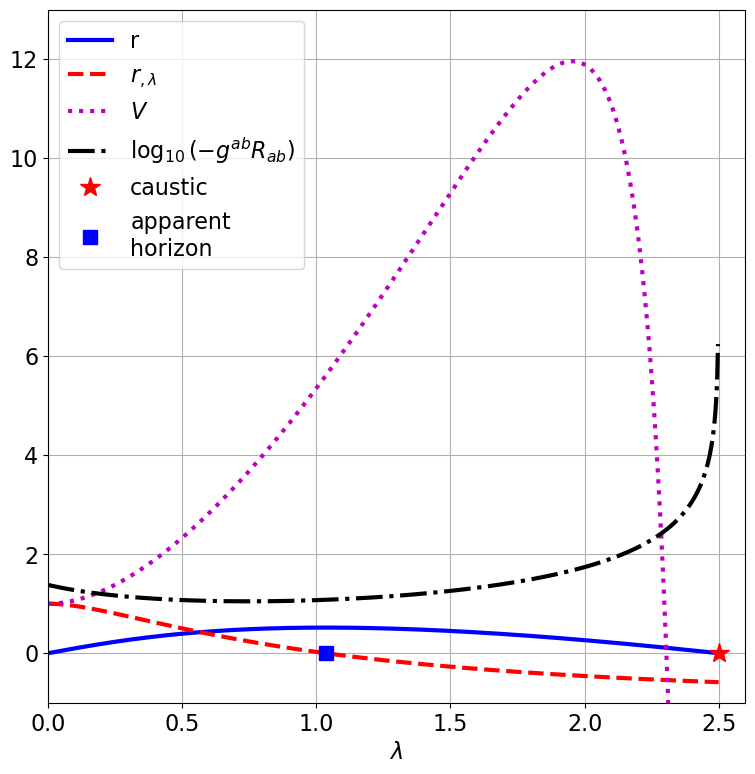
Figure 2: Inside event horizon initial data for $a=2.5(\sqrt{2}-1)$ and $b=\sqrt{2}$. The singular caustic is at $\lambda_{C}=2.5$ and the apparent horizon is at $\lambda_{A}=2.5(\sqrt{2}-1)\approx 1.04$.

IV From the physical field equations to their representation on a computer

IV.1 A generalized spatial grid

For the numerical simulations, we represent the affine parameter by a grid coordinate $x\in[-1,1]$ so that $\lambda=\lambda(x)$, while requiring $\lambda(-1)=0$ and $\lambda^{\prime}(-1)\neq 0$. With respect to the new grid variable (37) becomes

$$0 = r_{,xx}-(\ln|\lambda^{\prime}|)^{\prime}r_{,x}+\frac{r}{2}\Phi_{,x}^{2}$$ (58a)

$$L_{,x} = \frac{\lambda}{r}\Phi_{,x}$$ (58b)

$$\frac{Q_{,x}}{\lambda^{\prime}} = \frac{1}{\lambda^{2}}-\frac{1}{r^{2}}+\frac{1}{2}\left(\frac{L}{\lambda}\right)^{2}$$ (58c)

$$\Phi_{,u} = \frac{1+\lambda Q}{2\lambda^{\prime}}\Phi_{,x}+\frac{L}{2r}.$$ (58d)

Two grid functions $\lambda(x)$ are employed: (i) a linear grid function covering the finite $\lambda$ domain inside a black hole: and (ii) a compactified grid function covering the infinite $\lambda$ domain on an asymptotically flat null hypersurface.

IV.1.1 Linear grid function - interior region

The linear grid function

$$\lambda_{I}(x)=A(x+1),$$ (59)

with $A>0$, allows us to determine the fields for ${\lambda\in[0,2A]}$, The hierarchy (58) then becomes

$$0 = r_{,xx}+\frac{r}{2}\Phi_{,x}^{2}$$ (60a)

$$L_{,x} = \frac{A(x+1)}{r}\Phi_{,x}$$ (60b)

$$Q_{,x} = \frac{1}{A(1+x)^{2}}-\frac{A}{r^{2}}+\frac{1}{2A}\left[\frac{L}{(1+x)}\right]^{2}$$ (60c)

$$\Phi_{,u} = \frac{1}{2A}\left[1+A(1+x)Q\right]\Phi_{,x}+\frac{L}{2r}.$$ (60d)

The inner boundary conditions for the fields are

$$\begin{split}&r(-1)=0\;\;,\;\;r_{,x}(-1)=A\;\;,\;\;L(-1)=Q(-1)=0\;\;,\\ &\Phi_{,u}(-1)=\frac{1}{A}\Phi_{,x}(-1).\end{split}$$ (61)

In terms of the $x$ coordinate, ${r_{,\lambda}=r_{,x}/A}$ and

$$r_{,u}=\frac{1}{2}\left(\frac{A(1+x)}{r}+\frac{r_{,x}}{A}[1+A(1+x)Q]\right).$$

In order to start up the integration at $x=-1$ and enforce regularity at the origin, we numerically determine the derivative $\Phi_{(1)}(u)=\Phi_{,x}(u,-1)$ of the data at the origin. Then the right hand sides of (60b) - (60d) have the boundary values

$$L_{,x}|_{x=-1} =\Phi_{(1)}(u)$$ (62)

$$Q_{,x}|_{x=-1} =\frac{1}{3}\Phi_{(1)}^{2}(u)$$ (63)

$$\Phi_{,u}|_{x=-1} =\frac{1}{A}\Phi_{(1)}(u).$$ (64)

IV.1.2 Compactified grid function - exterior region

For the compactified grid function, we set

$$\lambda_{II}(x):=\lambda(x)=2A\frac{1+x}{1-x},$$ (65)

with $\lambda^{\prime}=4A(1-x)^{-2}$, which maps the infinite $\lambda$ domain into $(-1\leq x\leq+1)$

In order to regularize terms in (58) of the form $1/(1-x)^{k}$ which are singular at $x=1$ we introduce the auxiliary variable

$$R=(1-x)r,$$ (66)

with boundary values

$$r(u,\lambda=0)=0\;\;\;\rightarrow \;\;\;R(u,x=-1)=0$$ (67)

$$r_{,\lambda}(u,\lambda=0)=1\;\;\;\rightarrow \;\;\;R_{,x}(u,x=-1)=2A\;.$$ (68)

The derivatives of $r$ then transform into

$$r_{,\lambda}= \frac{(1-x)R_{,x}+R}{4A}$$ (69)

$$(1-x)r_{,u}= \frac{1}{2}\left\{\frac{1}{2A}[(1-x)R_{,x}+R]-\frac{A(1-x^{2})}{R}\right\}.$$ (70)

With these transformations, (58) becomes

$$0 = R_{,xx}+\frac{\Phi_{,x}^{2}}{2}R$$ (71a)

$$L_{,x} = \frac{2A(1+x)}{R}\Phi_{,x}$$ (71b)

$$Q_{,x} = \frac{1}{A(1+x)^{2}}-\frac{4A}{R^{2}}+\frac{1}{2A}\left[\frac{L}{(1+x)}\right]^{2}$$ (71c)

$$\Phi_{,u} = \frac{(1-x)}{2}\left\{\left[1-x+2A(1+x)Q\right]\frac{\Phi_{,x}}{4A}+\frac{L}{R}\right\}.$$

The right hand sides of (71b) - (LABEL:eq:dphidu_num_comp) have finite values at $x=-1$,

$$L_{,x}|_{x=-1} =\Phi_{(1)}(u)$$ (72)

$$Q_{,x}|_{x=-1} =\frac{4}{3}\Phi_{(1)}^{2}(u)$$ (73)

$$\Phi_{,u}|_{x=-1} =\frac{\Phi_{(1)}(u)}{A}.$$ (74)

V Some details on the numerical implementation

We solve the set of hypersurface-evolution equations using a pseudo-spectral method coupled with either an explicit second or third order scheme for the time evolution. We discretize the interval $-1\leq x\leq+1$ into $N+1$ Gauss-Lobatto points

$$x_{i}=-\cos\left(\frac{i\pi}{N}\right)\;\;,\;\;i=0,1,...,N.$$ (75)

The central time at the origin is discretized according to

$$u_{n}=u_{init}+n\Delta u,$$ (76)

where $u_{init}$ is the initial time and the time step $\Delta u$ is given by

$$\Delta u=\frac{u_{fin}-u_{init}}{(N-1)^{2}},$$ (77)

where $u_{fin}$ is the final evolution time. The scalar field $\Phi$ as well as

$$f\in\{r,L,Q,\Phi_{,u}\}$$ (78)

at a given time $u_{n}$ are represented by $N+1$ discrete values on the collocation points $x_{i}$,

$$f^{n}_{i}:=f(u_{n},x_{i})=\sum_{k=0}^{N}f_{k}(u_{n})T_{k}(x_{i})$$ (79)

where $T_{i}(x)$ are Chebysheff polynomials of the first kind.

In comparison to previous affine-null implementations CW2019 we use only one spatial domain of Gauss-Lobatto points and functions are expanded in Chebysheff polynomials of the first kind. Ref. CW2019 used a two domain spectral decomposition of the $\lambda$ axis and expanded fields in rational Chebysheff polynomials. Our approach uses half the number of Fast Fourier Transforms and matrix multiplications needed for the mapping between the Chebysheff coefficients and the functions evaluated at the collocation points. Another variation from CW2019 is the compactifiation of null infinity, as implemented in other characteristic codes 2002PhRvD..65h1501L ; Purrer:2004nq , the Pitt code 2012LRR….15….2W or the Spec code2015CQGra..32b5008H ; 2016CQGra..33v5007H .

The code is written in Python, in the framework of the anaconda package anaconda . Python performace is improved by employing the numba library lam2015numba and the BLAS/LAPACK wrappers of scipy 2020SciPy-NMeth .

The implementation of the spectral method follows the review of Townsend ; Olver_Slevinsky_Townsend_2020 . The initial null data for $\Phi$ are represented on the appropriate grid function (59) (for the interior of the event horizon) or (65) (for the exterior). We then solve the hypersurface equations (60) using (59) for the interior or (71) for the exterior using (65).

In order to regularize the right hand sides of (60) and (71), in particular (60c) and (71c)), near the origin $x=-1$ , we use a tenth order Taylor series to fill the values of the Gauss-Lobatto points inside a word tube $[-1\leq x\leq-1+\Delta x]$. The Taylor series coefficients were determined by successively applying a first order derivative operator on the data $\Phi(u_{n},x_{i})$ on complete $u_{n}=const$ null cones. An optimum value $\Delta x\approx 10^{-3}$ was found by numerical measurement of the ${\cal L}_{2}$ error norms given by (80)

$$\mathcal{L}_{2}(f)=\sqrt{\int_{-1}^{1}|f_{num}(x)-f_{ana}|^{2}dx}$$ (80)

of the fields $f$ defined in (78) between their numerical values, $f_{num}$, and their analytic expressions, $f_{ana}$, as given in (41), (44)-(45c) with $a=\sqrt{3}/2$ and $b=1/4$. Fig. 3 displays convergence of the ${\cal L}_{2}$ error norms for the fields $f$. The error in $\Phi_{,u}$, saturates at round-off error $\approx 2\cdot 10^{-14}$ for $N\leq 1000$ collocation points.

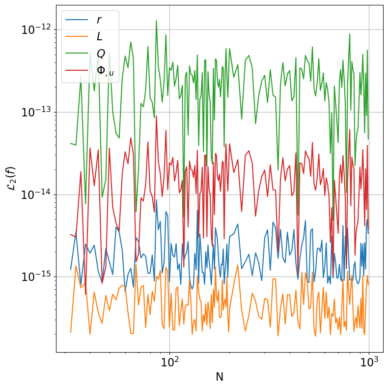
Figure 3: $\mathcal{L}_{2}$ error norms with respect to analytic initial data for the fields $f$ at different resolutions N.

As a time integrator for the evolution we use either second or third order Runge-Kutta schemes, in particular the (a.k.a Shu-Osher scheme 1988JCoPh..77..439S ) strong stability conserving Runge-Kutta methods SSPRK22 and SSPRK33 as presented in Hesthaven . Aliasing errors arising from high frequency pseudo spectral modes are controlled by a classical 2/3 filter. Fig. 4 displays the convergence of the point wise local error of the scalar field at central time $u=2.81$ with initial data parameter $a=1$ and $b=0.9$ using three different spatial resolutions. In particular, it shows the error of a high resolution run with 161 grid points with respect to two low resolution runs with either 41 or 81 grid points. It is seen that the two errors differ by a factor 1000 to 5000 indicating a temporal convergence that is better than the expected decay factor 8 for a third order method. The runs of Fig. 4 used the compactified grid function (65).

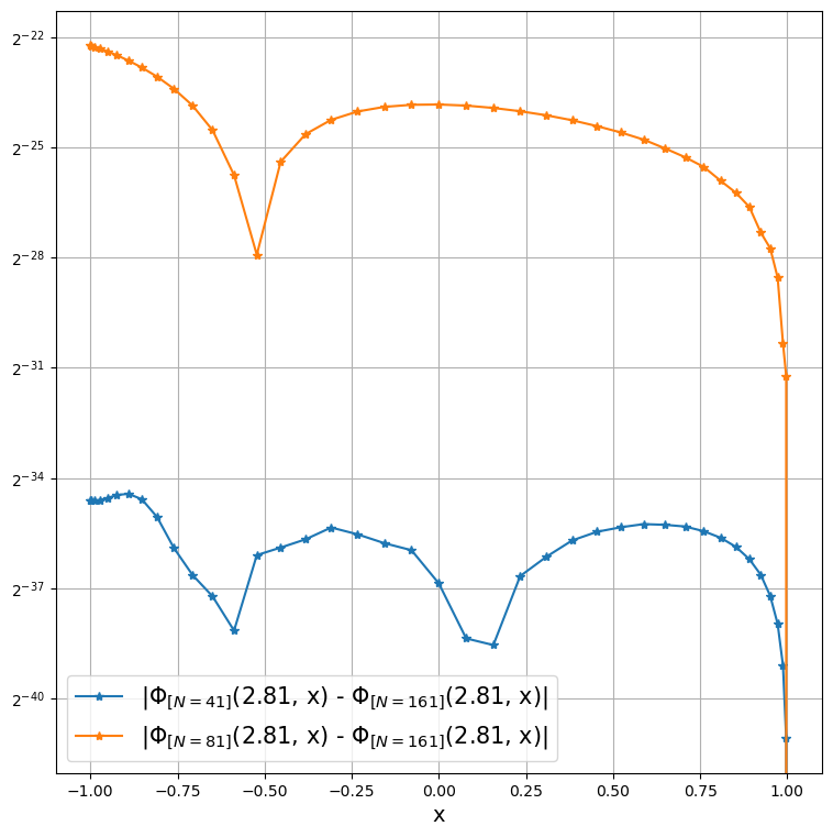
Figure 4: Absolute errors of the profile of $\Phi(u=2.81,x)$ when comparing low resolutions runs with $N\in\{41,81\}$ to a high resolution run with $N=161$ gridpoints.

An additional feature is the ability to track the position $\lambda_{A}$ of the apparent horizon. If at time $u_{[r_{,\lambda}=0]}$, $r_{,\lambda}$ changes sign, i.e. $r_{,\lambda}(u_{[r_{,\lambda}=0]},\lambda_{A})=0$, the $\lambda-$grid can be automatically adopted such that $\lambda_{A}$ corresponds to the outer boundary $x=1$ of the computational domain. For that purpose, the value of $\lambda_{A}$ is determined by a standard Newton-Raphson method using the $\lambda-$position of the midpoint between the maximum and minimum of $r_{,\lambda}$ as initial guesses. We then choose $A_{\lambda_{A}}=\lambda_{A}/2$ as the new parameter in the grid function (59). In turn, the data $\Phi(u_{[r_{,\lambda}=0]},x_{i})$ are mapped to the new grid using a cubic spline.

Our numerical implementation reproduces the standard features of the critical solution such as the universality and echoing (Fig. 5), scalar field dispersion (Fig. 6) and scalar field collapse (Fig. 7).

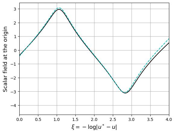
Figure 5: The echoing and universality shown for two different initial data sets: The black line corresponds to the initial data of CW2019 , i.e. $\Phi_{[12]}(0,\lambda)=\epsilon(1+\lambda^{2})^{-1}$ with $\epsilon=2.2731644$. The cyan dashed line corresponds the initial data (44) with $a=0.7$ and $b=0.947201675$. The echoing period is consistent with the Choptuik value $\Delta=3.44$, while the critical times are $u^{*}_{[12]}=2.2039$ and $u^{*}_{(3.4)}=2.165067$.

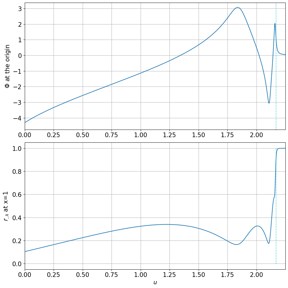
Figure 6: Standard behavior of the critical solutions: Subcritical initial data evolve toward the Minkowski value ${\lim_{\lambda\rightarrow\infty}r_{,\lambda}=H\rightarrow 1}$ and the scalar field disperses, $\Phi\rightarrow 0$, at time $u>u^{*}\approx 2.1$ (vertical dotted line).

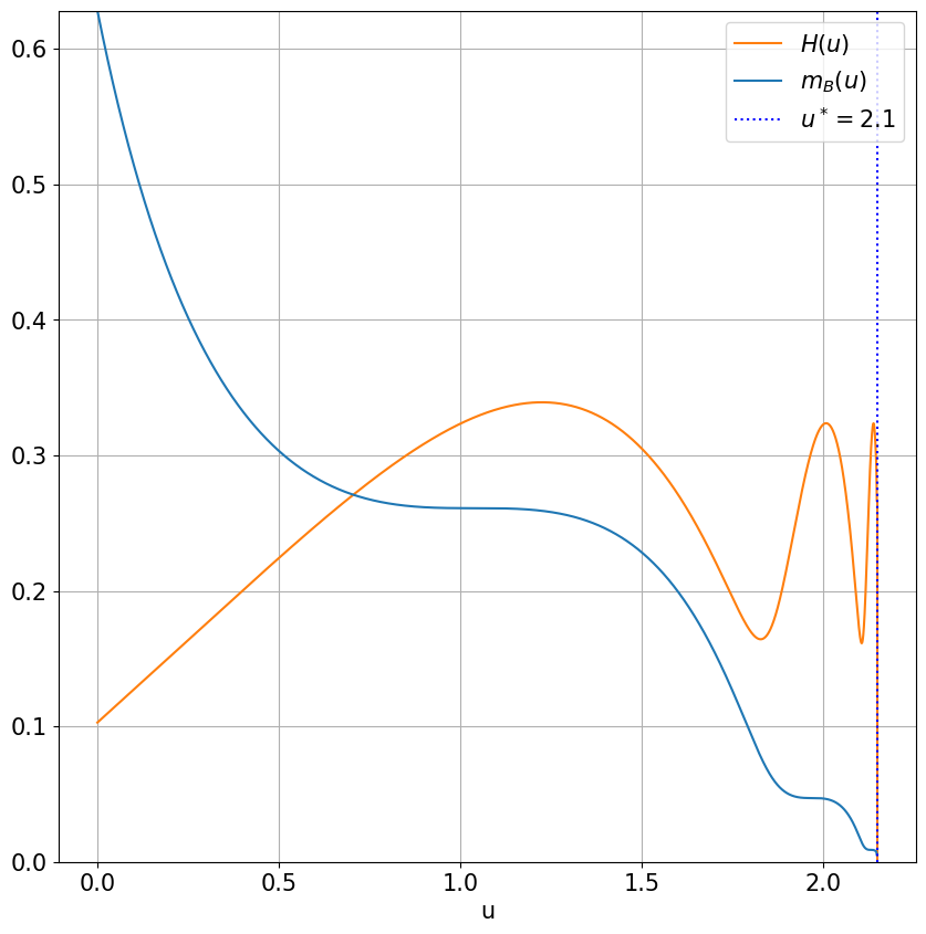
Figure 7: Standard behavior of the critical solutions: For supercritical initial data, the Bondi mass decays to a finite value and $H$ goes to zero for $u\rightarrow u^{*}\approx 2.1$ (vertical dotted line).

VI New results

VI.0.1 Scale symmetry

Systematic investigation of the 2-parameter initial data space (44) reveals the scale symmetry with respect to the parameter $a$ when studying critical phenomena. By a search of the parameter space $(a,b)$, we find that the critical parameter $b^{*}\approx 0.947202$ for all values of a. We also find that the critical time, $u^{*}$, has the simple relation $u^{*}\approx 3a$, as shown in Fig. 8. The linear dependence of the critical time $u^{*}$ on $a$ follows from the scaling properties of the field equations and initial data described in Sec. III.1. The factor $u^{*}/a\approx 3$ must be determined by numerical evolution. We are not aware of previous studies in which the critical time $u^{*}$ has such simple dependence on the initial data parameters. This explicit knowledge allows an estimate of the number of time steps needed to study critical collapse.

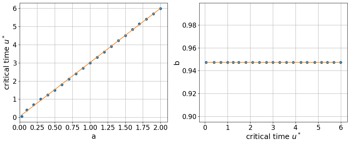
Figure 8: The dependence of the critical time $u^{*}$ on the initial data parameter $a$ (left plot) and $b$ (right plot) for initial data (44).

VI.0.2 Tracking the apparent horizon

To demonstrate that the system (37) can track the position of the apparent horizon, we use inside event horizon data with $b>1$. Because the position $\lambda_{A}$ of the apparent horizon moves inward towards the central geodesic and because the $\lambda$ domain shrinks in the process, we adaptively remap $\lambda_{A}$ to the outer boundary $x=1$ by adjusting the grid parameter $A$. This remapping is done after every time step and allows us to follow the motion of the apparent horizon close to the central world line. Fig. 9 shows temporal snapshots of radial profiles of $r$, the Misner-Sharp mass $m$, $r_{,\lambda}$ and the negative Ricci scalar for the evolution of the same inside event horizon initial data presented in Fig. 2. The apparent horizon is initially at $\lambda_{A}(u=0)=2.5(\sqrt{2}-1)\approx 1.04$. We follow the motion of the apparent horizon up until $\lambda_{A}(u=0.67)=0.05$. At this final time, the absolute value of the Ricci scalar $|g^{ab}R_{ab}|$ has risen by an order of magnitude over its value on the initial slice.

As the $\lambda$ grid shrinks towards the central world line, we confirm furthermore that the areal distance between the center and the apparent horizon decays. As expected from the relation $r(u,\lambda_{A})=2m(u,\lambda_{A})$, which follows from (13), this matches the decay of the Misner-Sharp mass $m$ of the apparent horizon shown in the upper plot of Fig. 10. The simulation was run successively with 101, 201, 401 and 801 grid points and numerical convergence was determined by comparing the positions $\lambda_{A}(u_{n})$ of the low resolution runs ($N\in\{101,201,401\}$) with the high resolution run $N=801$. We confirm the convergence of the second order time integrator, as the respective errors differ by a factor of 4 throughout the evolution (lower panel Fig. 10).

In Fig. 11, the position of the apparent horizon $\lambda_{A}$ can be read off from where $r_{,\lambda}=0$. Fig.  11 also shows that the profiles of $r$ and $2m$ intersect at the origin and then again at the position of apparent horizon.

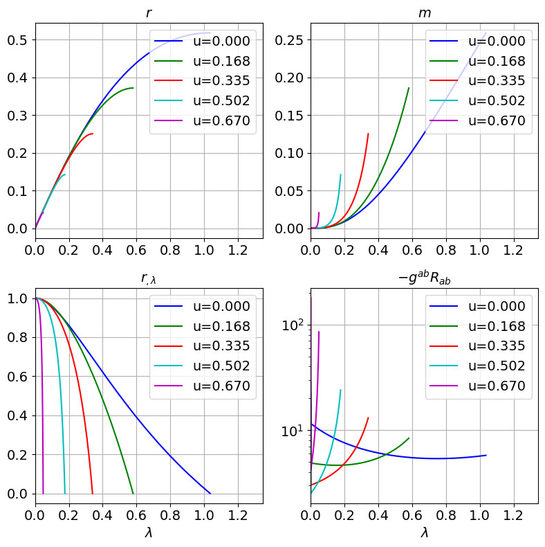
Figure 9: Snapshots of profiles of areal distance $r$ (upper left), Misner-Sharp mass $m$ (upper right), $r_{,\lambda}$ (lower left) and negative Ricci scalar (lower right) for inside event horizon initial data. Values at the endpoints of the curves correspond to values at the apparent horizon at the time indicated by the color in the legend.

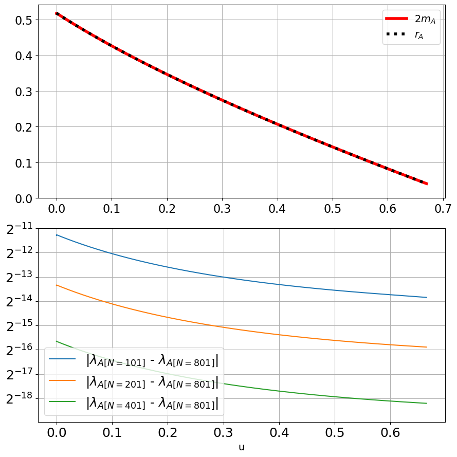
Figure 10: Upper panel: Confirmation of the relation $r=2m$ between the Misner-Sharp mass $m(u,\lambda_{A})$ and areal distance at the apparent horizon. The Misner-Sharp mass decays as the apparent horizon approaches the central worldline. Lower panel: Comparison of the absolute error of the position of the apparent horizon $\lambda_{A}(u)$ between low resolution runs ($N\in\{101,201,401\}$) and the high resolution run with $N=801$ grid points.

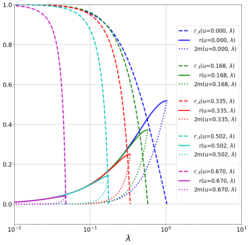
Figure 11: Snapshots of profiles of areal distance $r$ (solid lines), $r_{,\lambda}$ (dashed lines) and twice the Misner-Sharp mass $2m$ (dotted lines) between the origin and the apparent horizon. The profiles of $r$ and $2m$ intersect at the apparent horizon. The colors indicate the times of the snapshots as indicated in the legend.

VI.0.3 Evolution across the event horizon

For asymptotically flat supercritical initial data with $a=1$ and $b=0.95$, we are able to continue the evolution of asymptotically flat data across the event horizon up to the final collapse of the apparent horizon to the central worldline. For these simulations, we use the compactified grid function (65) with $A=1$ in the exterior region, where the $\lambda$ domain extends from the central world line to null infinity ${\cal I}^{+}$. At central time $u_{H}$, the time when the event horizon forms, $r$ approaches $2M_{B}$ as $\lambda$ goes to infinity. We determine $u_{H}\approx 2.027$ from the average of the time we detect a singular caustic on an outgoing null cone ($u_{C}=2.02813$) and the time of the last null cone that extends to ${\cal I}^{+}$ ($u=2.02687$). For times $u>u_{H}$, we excise the singular caustic and follow the motion of the apparent horizon using the linear grid function (59). Fig. 12 shows this adaptation of the grid function and grid parameter $A$ during the evolution of supercritical data.

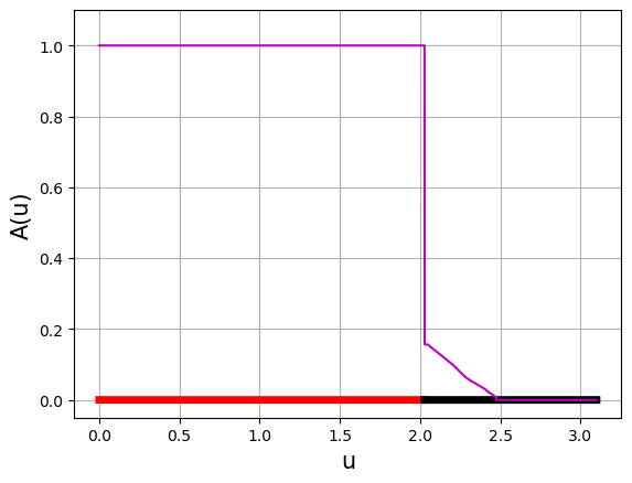
Figure 12: The red line indicates the use of the compactified grid function in the exterior of the event horizon and the black line the use of a linear grid function in the interior of the event horizon, during a supercritical run when the event horizon forms at $u_{H}\approx 2.027$. The magenta line indicates the change of the grid parameter $A$ from its initial value $A=1$ for $u<u_{H}$ and its decay towards zero for $u>u_{H}$ due to the remapping of the apparent horizon.

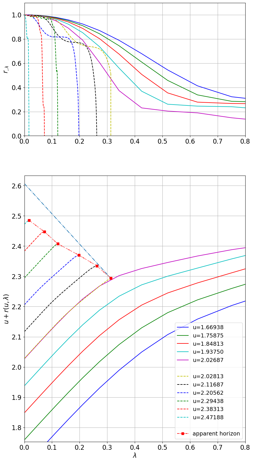
Figure 13: Temporal snapshots for supercritical initial data showing $r_{,\lambda}$ (top panel) and $u+r(u,\lambda_{A})$ (bottom panel) before and after event horizon formation at $u_{H}\approx 2.027$: In the lower panel, the locus of the apparent horizon (red dash dotted curve) lies below the tangent (blue dashed-dotted line) to the ingoing null ray at the position of the first detected apparent horizon. This is consistent with the spacelike nature of the apparent horizon. The color coded times in the legend apply to both panels.

Fig. 13, shows snapshots of the evolution in the domain $0\leq\lambda\leq 0.8$. The upper panel shows profiles of $r_{,\lambda}$ before and after event horizon formation at $u_{H}$. In the lower panel, for cleaner visualisation of the snapshots of $r(u,\lambda)$, we instead plot $u+r(u,\lambda)$ before and after event horizon formation. (Snapshots of $u+r$ rather than $r$ separate the profiles near the origin.) In both panels of Fig. 13, the solid lines are profiles in the exterior of the event horizon and the dashed lines in the interior, while the same colors correspond to profiles at the same times.

In the upper panel, $r_{,\lambda}$ decays for $u<u_{H}$, consistent with the increasing redshift between an exterior observer and the central worldline. For values $u\rightarrow u_{H}$ in Fig. 13, we see an inward motion of the positions on the $\lambda$-axis where ${r_{,\lambda}=0}$, i.e. the positions $\lambda_{A}(u)$ of the apparent horizon. In the lower panel of Fig. 13, the corresponding values of $u+r(u,\lambda_{A})$ are depicted by red squares. The dashed-dotted line connecting these squares indicate the locus of the apparent horizon. The blue dashed-dotted line Fig. 13 at $(\lambda,u+r)\approx(0.31,2.29)$ is the tangent to the ingoing null ray emanating from the position of the first detected apparent horizon. The locus of the apparent horizon lies below this ingoing null direction, consistent with the spacelike nature of the apparent horizon hypersurface.

In the lower panel of Fig. 13, all profiles of $u+r$ start from the center with the same slope $r_{,\lambda}(u,0)=1$, as required by the local Minkowski coordinate conditions at the origin. As $\lambda$ increases, the profiles deviate from straight lines and become concave due to the focusing of the null rays by the scalar field.

VII Summary

The Choptuik critical phenomena is a pristine problem in dynamic black hole formation. Here, we re-investigated the gravitational collapse of a massless scalar field in spherical symmetry using a characteristic formulation. In comparison with other studies 2002PhRvD..65h1501L ; Purrer:2004nq , which used the Bondi-Sachs metric MW2016 , we employed an affine-null metric. This allows numerical evolution beyond the formation of an event horizon where the areal coordinate $r$ in the Bondi-Sachs formalism becomes singular. An obstacle in implementing the affine-null formulation is that the main equations do not form a simple hierarchical scheme, as in the Bondi-Sachs formalism. However, the hierarchical structure has been restored for the general vacuum Einstein equations using a change in evolution variables Win2013 ; TM2019 , and this has been applied to the spherically symmetric Einstein-scalar field equations CW2019 . We adopted these variables here in the hierarchical system (31). However, although the affine-null coordinates remain non-singular up to the formation of physical singularities, there are individual terms in the system (31) which are infinite at the location of an apparent horizon, where $1/r_{,\lambda}\rightarrow\infty$. This is a limitation for applications of (31) to evolution in the interior of a black hole (as studied in Win2013 ; TM2019 ).

However, as shown in CW2019 , in spherical symmetry it is possible to regularize the system (31) such that it is free of the troublesome $1/r_{,\lambda}$ terms. This allows simulations of gravitational collapse to penetrate the event horizon. Here we took further advantage of this approach to implement an independent version of this regularized hierarchical system to explore the dynamics of the apparent horizon.

We verified the main results of CW2019 using a different pseudo-spectral method. In addition, we have shown that supercritical initial data could be evolved beyond the event horizon to the interior of the black hole (see Fig. 13). This evolution could be followed almost to the final singularity when the area of the apparent horizon approaches zero. The evolution of supercritical data demonstrated that the apparent horizon is a space-like hypersurface, in accord with analytic results. Analytic results using the affine-null system also showed that the final singularity is a space-like hypersurface. Our results led to the space-time picture Fig. 1 of supercritical gravitational collapse.

We also presented new null cone initial data (44) which is well suited for investigating both sub-critical and super-critical evolutions. For this initial data the hierarchy of hypersurface equations could be integrated to yield all metric and auxiliary functions in closed analytic form (see (45)). It is natural to ask if a regularized hierarchy such as (37) can be found for systems with less symmetry or different matter sources. A conclusive answer to this question is not in sight but under investigation.

VIII Acknowledgements

TM was supported by the FONDECYT de iniciación, 2019, No. 11190854. OB acknowledges a PhD scholarship of the University of Talca. HH is supported by the ANID PhD fellowship No. 21310374 of the Chilean government.

References

- (1) M. W. Choptuik, “Universality and scaling in gravitational collapse of a massless scalar field,” Phys. Rev. Lett. , vol. 70, pp. 9–12, Jan. 1993.
- (2) C. Gundlach, “Choptuik Spacetime as an Eigenvalue Problem,” Phys. Rev. Lett. , vol. 75, pp. 3214–3217, Oct. 1995.
- (3) S. Hod and T. Piran, “Critical behavior and universality in gravitational collapse of a charged scalar field,” Phys. Rev. D, vol. 55, pp. 3485–3496, Mar. 1997.
- (4) R. S. Hamadé and J. M. Stewart, “The spherically symmetric collapse of a massless scalar field,” Classical and Quantum Gravity, vol. 13, pp. 497–512, Mar. 1996.
- (5) M. Reiterer and E. Trubowitz, “Choptuik’s Critical Spacetime Exists,” Communications in Mathematical Physics, vol. 368, pp. 143–186, May 2019.
- (6) C. Gundlach, “Understanding critical collapse of a scalar field,” Phys. Rev. D, vol. 55, pp. 695–713, Jan. 1997.
- (7) E. W. Hirschmann and D. M. Eardley, “Universal scaling and echoing in the gravitational collapse of a complex scalar field,” Phys. Rev. D, vol. 51, pp. 4198–4207, Apr. 1995.
- (8) C. Gundlach and J. M. Martín-García, “Critical Phenomena in Gravitational Collapse,” Living Reviews in Relativity, vol. 10, p. 5, Dec. 2007.
- (9) J. M. Martín-García and C. Gundlach, “Global structure of Choptuik’s critical solution in scalar field collapse,” Phys. Rev. D, vol. 68, p. 024011, July 2003.
- (10) D. Garfinkle, “Choptuik scaling in null coordinates,” Phys. Rev. D, vol. 51, pp. 5558–5561, 1995.
- (11) M. Purrer, S. Husa, and P. C. Aichelburg, “News from critical collapse: Bondi mass, tails and quasinormal modes,” Phys. Rev. D, vol. 71, p. 104005, 2005.
- (12) J. A. Crespo, H. P. de Oliveira, and J. Winicour, “Affine-null formulation of the gravitational equations: Spherical case,” Phys. Rev. D, vol. 100, p. 104017, Nov. 2019.
- (13) C. Lechner, J. Thornburg, S. Husa, and P. C. Aichelburg, “New transition between discrete and continuous self-similarity in critical gravitational collapse,” Phys. Rev. D, vol. 65, p. 081501, Apr. 2002.
- (14) J. Winicour, “Affine-null metric formulation of Einstein’s equations,” Phys. Rev. D, vol. 87, p. 124027, June 2013.
- (15) J. Winicour, “Characteristic Evolution and Matching,” Living Reviews in Relativity, vol. 15, p. 2, Jan. 2012.
- (16) C. J. Handmer and B. Szilágyi, “Spectral characteristic evolution: a new algorithm for gravitational wave propagation,” Classical and Quantum Gravity, vol. 32, p. 025008, Jan. 2015.
- (17) C. J. Handmer, B. Szilágyi, and J. Winicour, “Spectral Cauchy characteristic extraction of strain, news and gravitational radiation flux,” Classical and Quantum Gravity, vol. 33, p. 225007, Nov. 2016.
- (18) T. Mädler, “Affine-null metric formulation of general relativity at two intersecting null hypersurfaces,” Phys. Rev. D, vol. 99, p. 104048, May 2019.
- (19) T. Mädler and E. Gallo, “Slowly rotating Kerr metric derived from the Einstein equations in affine-null coordinates,” Phys. Rev. D, vol. 107, p. 104010, May 2023.
- (20) E. Gallo, C. Kozameh, T. Mädler, O. M. Moreschi, and A. Perez, “Spherically symmetric black holes and affine-null metric formulation of Einstein’s equations,” Phys. Rev. D, vol. 104, p. 084048, Oct. 2021.
- (21) T. Mädler and E. Müller, “The Bondi-Sachs metric at the vertex of a null cone: axially symmetric vacuum solutions,” Classical and Quantum Gravity, vol. 30, p. 055019, Mar. 2013.
- (22) H. Bondi, M. G. J. van der Burg, and A. W. K. Metzner, “Gravitational Waves in General Relativity. VII. Waves from Axi-Symmetric Isolated Systems,” Proceedings of the Royal Society of London Series A, vol. 269, pp. 21–52, Aug. 1962.
- (23) L. A. Tamburino and J. H. Winicour, “Gravitational Fields in Finite and Conformal Bondi Frames,” Physical Review, vol. 150, pp. 1039–1053, Oct. 1966.
- (24) T. Mädler and J. Winicour, “The sky pattern of the linearized gravitational memory effect,” Classical and Quantum Gravity, vol. 33, p. 175006, Sept. 2016.
- (25) “Anaconda software distribution,” 2020.
- (26) S. K. Lam, A. Pitrou, and S. Seibert, “Numba: A llvm-based python jit compiler,” in Proceedings of the Second Workshop on the LLVM Compiler Infrastructure in HPC, pp. 1–6, 2015.
- (27) P. Virtanen, R. Gommers, T. E. Oliphant, M. Haberland, T. Reddy, D. Cournapeau, E. Burovski, P. Peterson, W. Weckesser, J. Bright, S. J. van der Walt, M. Brett, J. Wilson, K. J. Millman, N. Mayorov, A. R. J. Nelson, E. Jones, R. Kern, E. Larson, C. J. Carey, İ. Polat, Y. Feng, E. W. Moore, J. VanderPlas, D. Laxalde, J. Perktold, R. Cimrman, I. Henriksen, E. A. Quintero, C. R. Harris, A. M. Archibald, A. H. Ribeiro, F. Pedregosa, P. van Mulbregt, and SciPy 1.0 Contributors, “SciPy 1.0: Fundamental Algorithms for Scientific Computing in Python,” Nature Methods, vol. 17, pp. 261–272, 2020.
- (28) S. Olver and A. Townsend, “A fast and well-conditioned spectral method,” SIAM Review, vol. 55, no. 3, pp. 462–489, 2013.
- (29) S. Olver, R. M. Slevinsky, and A. Townsend, “Fast algorithms using orthogonal polynomials,” Acta Numerica, vol. 29, p. 573–699, 2020.
- (30) C.-W. Shu and S. Osher, “Efficient Implementation of Essentially Non-oscillatory Shock-Capturing Schemes,” Journal of Computational Physics, vol. 77, pp. 439–471, Aug. 1988.
- (31) J. S. Hesthaven, S. Gottlieb, and D. Gottlieb, Spectral methods for time-dependent problems. Cambridge University Press, 2007.
- (32) T. Mädler and J. Winicour, “Bondi-Sachs Formalism,” Scholarpedia, vol. 11, p. 33528, Dec. 2016.