Can Graph Learning Improve Task Planning?

Abstract

Task planning is emerging as an important research topic alongside the development of large language models (LLMs). It aims to break down complex user requests into solvable sub-tasks, thereby fulfilling the original requests. In this context, the sub-tasks can be naturally viewed as a graph, where the nodes represent the sub-tasks, and the edges denote the dependencies among them. Consequently, task planning is a decision-making problem that involves selecting a connected path or subgraph within the corresponding graph and invoking it. In this paper, we explore graph learning-based methods for task planning, a direction that is orthogonal to the prevalent focus on prompt design. Our interest in graph learning stems from a theoretical discovery: the biases of attention and auto-regressive loss impede LLMs’ ability to effectively navigate decision-making on graphs, which is adeptly addressed by graph neural networks (GNNs). This theoretical insight led us to integrate GNNs with LLMs to enhance overall performance. Extensive experiments demonstrate that GNN-based methods surpass existing solutions even without training, and minimal training can further enhance their performance. Additionally, our approach complements prompt engineering and fine-tuning techniques, with performance further enhanced by improved prompts or a fine-tuned model .

1 Introduction

LLM-empowered autonomous agents have recently emerged as a rapidly growing field of research and are considered a significant step towards artificial general intelligence (AGI) [43, 4]. These agents have achieved remarkable successes across a variety of domains, as evidenced by their ability to address complex AI challenges (e.g., HuggingGPT [31] and Visual ChatGPT [46]), excel in gaming environments (e.g., Voyager [40]), and drive innovation in chemical research (e.g., [3]). Within this burgeoning field, task planning emerges as a critical area of study. It involves LLMs autonomously interpreting user instructions, breaking these instructions down into concrete and solvable sub-tasks, and then fulfilling the user’s request by executing each sub-task [29, 31, 30]. For instance, in the case of HuggingGPT [31], task planning involves invoking expert AI models from the HuggingFace website to solve complex AI tasks beyond the capabilities of GPT alone.

Given its practical significance, numerous algorithms have been proposed, with a major focus on prompt design [30, 31, 23, 20, 42, 34, 53, 2, 45]. This paper proposes to explore an orthogonal direction, i.e., graph-learning-based approaches. In task planning, solvable sub-tasks can be naturally represented as a task graph, wherein each node corresponds to a distinct sub-task, and each edge signifies the dependencies between these sub-tasks. The crux of task planning, therefore, involves selecting a connected path or subgraph to satisfy the user’s request, which is a decision-making problem on graphs. Adopting this framework, we analyze the task planning capabilities of LLMs, specifically within the context of HuggingGPT [31]. Our empirical investigation uncovers that a considerable portion of planning failures can be ascribed to the LLMs’ inefficacy in accurately discerning the structure of the task graph. This finding presents intriguing questions from both theoretical and empirical perspectives. Theoretically, it initiates a discussion on the inherent limitations of LLMs in processing graph-based tasks. Empirically, it highlights the urgent need for developing effective and efficient strategies to mitigate this deficiency and improve task planning performance.

For the theoretical question, we first investigate the expressiveness of Transformer architectures when applied to graph tasks with sequential graph input, such as edge list representations. Our initial hypothesis is that the format of sequential graph input might not align with the inductive bias inherent to graph structures, potentially reducing expressiveness. Contrary to this hypothesis, it is proved that by taking edge lists as the input, a constant-width Transformer can solve graph decision-making problems by simulating dynamic programming algorithms on edge lists. Nevertheless, we find that LLMs’ solutions lack invariance under graph isomorphism, an important property for graph decision-making problems. In addition, the expressiveness is weakened if the attention is sparse, which is typically observed in LLMs [48]. Beyond expressiveness, we also examine the influence of auto-regressive loss, demonstrating that it introduces spurious correlations that can be harmful to graph decision-making tasks. These insights expose the inherent limitations of LLMs in task planning and, more broadly, in graph-related problems (e.g., the challenges in [10, 41, 24]).

To tackle the limitations, we take the use of GNNs, which have been shown to adeptly handle graph decision-making problems, both in theory and in practice [16, 50]. Initially, we deploy LLMs to interpret an ambiguous user request, breaking it down into more detailed steps. Subsequently, we utilize a GNN to retrieve the relevant sub-tasks based on these detailed steps and the corresponding sub-task descriptions. Notably, this approach can be implemented without training if we adopt parameter-free GNN models such as SGC [47]. In the case of training-based methods, we apply the Bayesian Personalized Ranking (BPR) loss [27] to facilitate learning from the implicit sub-task rankings. Extensive experiments demonstrate that the proposed methods achieve better performance than baselines. Specifically, our main contributions are summarized as follows:

1. Task Planning Formulation: This study presents a formulation of task planning as a graph decision-making problem. In the realm of task planning, our work initiates the exploration of graph learning methodologies to enhance performance. Concurrently, it introduces task planning as a new application in the graph learning domain.

2. Theoretical Insights: We prove that Transformers have expressiveness to solve graph decision-making problems based on edge list input, but inductive biases of attention and the auto-regressive loss function may serve as obstacles to their full potential.

3. Novel Algorithms: Based on the theoretical analysis, we introduce an additional GNN for sub-task retrieval, available in both training-free and training-based variants. The experiments on diverse LLMs and planning datasets demonstrate that the proposed method outperforms existing solutions with much less computation time. Furthermore, the performance is further enhanced by improved prompts or a fine-tuned model.

2 Preliminaries and Formulations

In this section, we introduce the task planning and GNNs. More importantly, we connect them with the classic concepts, i.e., decision-making problems and dynamic programming. This connection will play a pivotal role in the theoretical analysis and algorithm development.

2.1 Task Planning and Decision Making

In task planning, the input comprises an ambiguous user request along with a pool of available sub-tasks. The output is a selection of specific sub-tasks to be invoked and the manner in which they are to be executed. An illustrative example within HuggingGPT is depicted in Figure 1.

The sub-tasks form a task graph $G=(V,E)$ [30], where the nodes $V=\{v_{1},\cdots,v_{n}\}$ represent a set of solvable tasks, and an edge from $v_{i}$ to $v_{j}$ is established if the sub-task $v_{j}$ is dependent on the sub-task $v_{i}$. The goal of task planning is to identify a path or a connected sub-graph within the task graph that fulfills the users’ requests. In the context of HuggingGPT [31], the nodes correspond to expert AI models from the HuggingFace website. An edge is drawn from $v_{i}$ to $v_{j}$ if the input format of $v_{j}$ matches the output format of $v_{i}$. Task planning involves invoking a sequence of AI models (i.e., a path). Viewed from this angle, task planning bears resemblance to traditional decision-making problems on graphs, such as planning for the shortest path. The key distinction from classic decision-making problems lies in the specification of the objective value: it is explicitly defined in the former, while in task planning, it is implicitly inferred from the users’ requests.

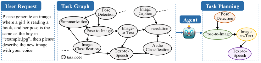
Figure 1: Illustration of Task Planning in HuggingGPT.

2.2 GNNs and Dynamic Programming

GNNs are a class of neural networks preserving equivariance under graph isomorphism. The most popular GNNs are based on message passing scheme, where the node representation is iteratively updated by aggregating the representations from its neighbors. Formally, the $k$-th layer of a GNN is given by

$$\bm{m}_{u}^{(k)}=\text{Aggregate}^{(k)}(\{[\bm{h}_{v}^{(k-1)},\bm{e}_{u,v}]|v\in\mathcal{N}(u)\}),\quad\bm{h}_{u}^{(k)}=\text{Combine}^{(k)}(\bm{h}_{u}^{(k-1)},\bm{m}^{(k)}_{u}),$$ (1)

where $\mathcal{N}(u)$ denotes the set of in-neighbors of node $u$, $\bm{e}_{u,v}$ is the edge feature, and $\bm{h}_{u}^{(k)}$ is the representation of node $u$ with $\bm{h}_{u}^{(0)}$ representing initial node features. The aggregation function $\text{Aggregate}^{(k)}$ and update function $\text{Combine}^{(k)}$ are parameterized by neural networks and the choice of these two functions leads to different types of GNNs.

DP [1] presents a general framework for solving decision-making problems. It breaks a complex problem into simpler sub-tasks, each of which can be solved based on the results of previous sub-tasks. The general form of DP is expressed as

$$\text{Answer}[k][i]=f\left(\square_{j\in\mathcal{T}(i)}(\text{Answer}[k-1][j]\oplus c[i][j])\right),$$ (2)

where $\text{Answer}[k][i]$ is the solution to state $i$ in the $k$-th iteration, $f$ is a task-specific update function, $c[i][j]$ is a cost associated with state $i$ and $j$, $\mathcal{T}(i)$ is the set of state can be transited to $i$, $\square_{j\in\mathcal{T}(i)}$ is an aggregation function such as MAX or SUM, $\oplus$ is an operator such as + or XOR. We give the formulation of typical DP algorithms in Appendix C.1. DP updates in (2) can be expressed by GNNs’ updates in Eq. (1) if we set the states as the nodes, $\mathcal{N}(u)=\mathcal{T}(u)$, and $\bm{e}_{u,v}=c[u][v]$. More formal relationships are established in [50, 7], showing that GNNs are well-suited for solving DP problems.

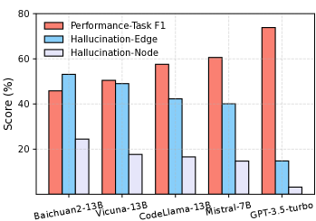
Figure 2: Illustration of performance and hallucination ratio across LLMs.

3 Diagnosing Task Planning in LLMs

3.1 Empirical Observations

We adopt the experimental settings as outlined in the work of HuggingGPT [31], where the prompts are specifically optimized for task planning on HuggingFace. The evaluation metric calculates the F1 score to assess the accuracy of the tasks identified by LLMs against the ground-truth tasks. Additionally, we report two task-graph-related metrics: the node hallucination ratio and the edge hallucination ratio. These metrics measure the frequency of non-existent nodes (i.e., tasks) and edges (i.e., relations) outputted by LLMs, respectively, indicative of the models’ misinterpretation of the graph input.

Our empirical findings reveal that (1) LLMs exhibit a certain hallucination ratio, and (2) there is a strong correlation between the hallucination ratio and planning performance. This suggests that LLMs struggle to accurately interpret the task graph while the task graph is the key to the performance.

3.2 Theoretical Insights

Besides the example mentioned above, existing studies demonstrate that LLMs struggle with understanding graph-structured inputs [41, 10]. Despite these empirical evaluations, there remains a limited theoretical understanding of this phenomenon. In this subsection, we explore the performance of LLMs in graph decision-making problems, including task planning. In contrast to previous graph learning approaches for graph decision-making problems, LLMs process the graph input by flattening it into a sequence and are trained using an auto-regressive loss. We will then examine the impact of these two factors.

Sequential Graph Input: We consider general graph decision-making problems that can be resolved using DP as described in (2). The input comprises the edge list and initial states:

$$\underbrace{u_{1}\ v_{1}\ c[u_{1}][v_{1}]\ u_{1}\ v_{2}\ c[u_{1}][v_{2}]\ \ldots}_{\text{edge list}}\ \underbrace{u_{1}\ \text{Answer}[0][u_{1}]\ \ldots\ u_{n}\ \text{Answer}[0][u_{n}]}_{\text{initial states}}$$ (3)

The intended output format is $u_{1}\ \text{Answer}[k][u_{1}]\ \ldots\ u_{n}\ \text{Answer}[k][u_{n}]$. To our surprise, although the edge list input does not directly reflect the geometric structures of graphs, it enables Transformers to simulate DP efficiently, in terms of expressiveness, as demonstrated by the following theorem.

Theorem 1.

(Expressiveness) Assume the input format is given in (3) and $f,\oplus,\square$ in DP update (2) satisfy the assumptions 1 and 2. There exists a log-precision constant-depth and constant-width Transformer that simulates one step of DP update in (2). As a consequence, there exists a log-precision $O(k)$-depth and constant-width Transformer that simulates $k$ steps of DP update in (2).

The proof is presented in Appendix B.1. However, certain aspects of the proof’s constructions are challenging to be realized in Transformers that have been pretrained on natural language. First, the embedding process must be carefully filtered to ensure invariance under graph isomorphism. This invariance property does not align with the inductive biases inherent in natural language, making it difficult to achieve. Consequently, if an LLM can accurately produce the correct answer for a specific ordering of nodes, it might not maintain this accuracy after the nodes have been reordered (experiments given in Appendix C.2). Second, each token needs to synchronize its hidden states with all other tokens sharing the same token ID, which is of order $O(|V|)$. In practice, the attention trained from natural language is typically sparse [48], leading to intractability issues. The formal lower bound is provided in the following proposition and the proof is given in Appendix B.2.

Proposition 1.

Assume the input format is described (3) and that the attention mechanism is limited to attending to a constant number of tokens. There exists at least one instance of one-step DP update such that no log-precision constant-width constant-depth transformer can simulate.

Auto-regressive Loss: Our investigation next focuses on the auto-regressive loss and considers the following scenario: given a fixed task graph, user data is collected to perform instruction tuning with next-token-prediction loss. A question arises concerning whether auto-regressive loss might introduce spurious correlations harmful to planning problems. We conceptualize this issue through the lens of a path-planning problem. The training dataset comprises input sequences of the form $s\ t\ s\ v_{1}\ v_{2}\ \cdots\ t$, where $s$ represents the source node, $t$ the target node, and the sequence $s\ v_{1}\ v_{2}\ \cdots\ t$ is a path that adheres to specified constraints. During testing, given the initial and target nodes $s$ and $t$, the model is expected to generate a path with the same constraint. Our findings indicate that auto-regressive loss can lead to the emergence of a frequency-based spurious correlation, as substantiated by the following theorem and the proof is given in Appendix B.3.

Theorem 2.

(Spurious correlations of auto-regressive loss) Assume (1) the loss employed is a next-token-prediction loss utilizing cross-entropy, applied to the sub-sequence $v_{1}\ v_{2}\ \cdots\ t$ during training; (2) the output logits are determined by target node $t$ and the current node $v_{i-1}$. Let $N_{t,v_{i-1},u}$ be the number of times in the training dataset such that $t$ is the target node, $v_{i-1}$ is the current node and $v_{i}=u$ is the next node. The optimal logits for predicting the next node $u$ from current node $v_{i-1}$ towards target node $t$ is given by $\hat{\bm{v}}_{i}[u]=\frac{N_{t,v_{i-1},u}}{\sum_{u}N_{t,v_{i-1},u}}$ if $\sum_{u}N_{t,v_{i-1},u}>0$. If $\sum_{u}N_{t,v_{i-1},u}=0$, $\hat{\bm{v}}_{i}[u]$ can be any non-negative number subject to $\sum_{u}\hat{\bm{v}}_{i}[u]=1$.

In our setup, $s$ $t$ is the instruction and the third token is a duplicate of the first token. It is reasonable to exclude these tokens in the loss calculation, which is the first assumption. The second assumption assumes that the output only depends on the current node and target node, which is a minimal requirement for path-related problems. For DP problems, the frequency-based prediction contradicts to the value-based ground-truth. We then give an example that auto-regressive loss even cannot find a valid path.

Example 1.

Consider a training dataset consisting of a sufficient number of valid paths. Suppose the dataset contains two paths $a\ b\ c$ and $b\ c\ d$ and there are no other paths such that $t=d$ and the current node $v_{i}=a$ for all $i$. Then we have $N_{d,a,u}\equiv 0$ for all $u$ and the logits for the next node can be arbitrary. This results in the model’s inability to predict the next node of $a$ when given $a$ as the source node and $d$ as the target node.

For a human, finding a path from $a$ to $d$ simply involves concatenating the paths $a\ b\ c$ and $b\ c\ d$. However, auto-regressive loss fails under such circumstances. In task planning datasets, we indeed observe that the performance of finetuned LLMs is inferior to that of GNNs trained on the same dataset, as shown in Figure 3(b).

4 A Simple Fix: Introducing GNNs

In contrast to LLMs, GNNs can strictly operate on the task graph, thereby avoiding hallucinations. Additionally, they leverage the graph structure as input, rather than flattening the graph into a sequence, thus overcoming the theoretical limitations discussed previously. Furthermore, GNNs have demonstrated proficiency in handling graph decision-making problems, both theoretically and empirically [50, 7, 16]. As a result, the simplest fix is to integrate GNNs into the task-planning algorithm. In this section, we first briefly introduce the current LLM-based solutions and then illustrate how GNNs can be integrated into them. We propose both training-free and training-based approaches to enhance performance. Training-free methods are necessary when the available tasks are continuously changing, or new tasks are emerging consistently. This scenario is common when the task planning module is deployed in a new system. Once the task planning module has been deployed for a period, it becomes possible to collect users’ requests and label a small proportion of the data, enabling lightweight training-based methods.

4.1 Purely LLM-based Task Planning

We outline a two-stage pipeline for task planning adopted in HuggingGPT [30, 31]. The first stage involves request decomposition, where a user’s ambiguous request is broken down into concrete steps via LLMs. For instance, the request illustrated in Figure 1 is decomposed into the following steps: (1) analyze the pose of the boy; (2) take that pose and generate a new image; (3) generate the caption for newly generated image; (4) convert the generated text into audio. The second stage is task retrieval. For each decomposed step, LLMs are employed to retrieve an appropriate task from the task pool and execute them in sequence.

4.2 A Training-free GNN-based Approach

We introduce GNNs into the task retrieval stage by formulating it as a node classification problem. The node embedding is the embedding of this node’s description. For example, the node description in HuggingFace can be “Translation. Translation is the task of converting text from one language to another”. Given that the node description is usually simple, node embedding is obtained by e5-355M [44] for efficiency. Then we use the parameter-free GNN (i.e., SGC [47]) to refine the node embeddings. The update is given by $\bm{H}^{(k)}=\alpha\bm{H}^{(k-1)}+(1-\alpha)\hat{\bm{A}}\bm{H}^{(k-1)}$, where $\bm{H}^{(k)}$ is the embedding after $k$-layer SGC, $\bm{H}^{(0)}$ is the initial node feature, $\hat{\bm{A}}$ is the normalized adjacency matrix of the task graph, and $\alpha$ is a hyperparameter.

When selecting the task node for a step $s_{i}$, e5-355M is used to embed the LLMs’ generated step as $\bm{x}_{i}^{\text{step}}$. Given a sequence of previously selected task nodes $\{v_{1},\cdots,v_{i-1}\}$, the next node $v_{i}$ is chosen according to $v_{i}=\text{argmax}_{v\in\mathcal{N}(v_{i-1})}\;\langle\bm{h}_{v},\bm{x}_{i}^{\text{step}}\rangle$, where $\bm{h}_{v}$ is the node embedding. Particularly, $v_{1}$ can be selected from the whole graph. The one-by-one node selection approach is inspired by the traditional research of GNNs for decision-making problems like combinatorial optimization [16].

4.3 A Training-required GNN-based Approach

The inference process in training-required methods mirrors that of the training-free approach, with the difference being the substitution of parameter-free GNNs with parametric counterparts, such as GAT [39] or GraphSAGE [11]. Here we specify the training process of GNNs.

Data Preparation: We assume that each entry in the task planning dataset comprises a user request, a sequence of decomposed steps, and the corresponding ground-truth tasks, denoted as $(\text{request},\{s_{1},\ldots,s_{n}\},\{v_{1},\ldots,v_{n}\})$. If the dataset does not adhere to this format, we reformat it accordingly using GPT-4, with details provided in Appendix E.2. It is important to note that there is a one-to-one correspondence between the steps and tasks in the dataset. The node classification dataset is represented as $\{s_{i},v_{i}\}_{i=1}^{n}$, where $s_{i}$ is a step described in natural language, and $v_{i}$ is its corresponding task.

Training Loss: Inspired by GNN for recommendation [12], we adopt the Bayesian Personalized Ranking (BPR) loss [27] designed for recommendation with binary rankings. The loss function is given by

$$\ell=\sum_{(\bm{x}^{\text{step}},v,v^{\prime})}-\log\;\sigma(\langle\bm{h}_{v},\bm{x}^{\text{step}}\rangle-\langle\bm{h}_{v^{\prime}},\bm{x}^{\text{step}}\rangle),$$

where $\bm{x}^{\text{step}}$ represents the embedding of the step’s textual description generated by e5-355M, $v$ is ground-truth task, and $v^{\prime}$ is a negative task. We select negative tasks that are textually similar to the positive task, and for computational efficiency, we limit our selection to $2$ negative tasks per positive task. The trainable parameters may merely include GNNs or both GNNs and e5-355M.

5 Experiments and Analysis

5.1 Experimental Setup

Datasets: We utilize four datasets across two task planning benchmarks: HuggingFace tasks, Multimedia tasks, and Daily Life API tasks from TaskBench [30], as well as TMDB API tasks from RestBench [35]. The HuggingFace dataset includes AI models on the HuggingFace. The Multimedia dataset provides a wide range of user-centric tasks, such as file downloading and video editing. The Daily Life APIs cater to everyday services like web search and shopping functionalities. TMDB focuses on movie-related search and retrieval tasks. Statistics for each dataset are presented in Table 5 with illustrative examples shown in Figure 8 in Appendix. Other benchmarks, such as ToolBench [25] and ToolAlpaca [38], are less suitable for our experiments due to (1) the absence of a well-defined task graph detailing tasks and their dependencies, and (2) a scarcity of samples involving multi-task planning, with a focus on single-task retrieval.

Evaluation: For the datasets from TaskBench, we split $3000$ samples for training and $500$ samples for testing, each containing an invocation path with at least two tasks. For the TMDB dataset, we first filter to include the samples with two or more invoked tasks, and then randomly select a sample served as the in-context learning example. The remaining $94$ samples are designated for testing. We adopt the evaluation metric in TaskBench [30] and HuggingGPT [31], i.e., Node F1-Score (n-F1) and Link F1-Score (l-F1), which measure the accuracy of invoked tasks and invoked dependencies, respectively. We also measure the token consumption (# tok) as the efficiency metric.

Choices of LLMs: We consider close-sourced LLMs, i.e., GPT-3.5-turbo and GPT-4-turbo, as well as open-sourced LLMs with different parameter scales, including CodeLlama-13B(or 7B)-Instruct-hf [28], Mistral-7B-Instruct-v0.2 [15], Vicuna-13B-v1.5 [54], and Baichuan2-13B-Chat [51].

Choices of GNNs: To comprehensively investigate the effectiveness of different graph learning methods in enhancing task planning, we consider a wide range of graph neural networks, including SGC [47], GCN [18], GAT [39], GraphSAGE [11], GIN [49], and TransformerConv [32].

5.2 Performance of the Training-free Approach

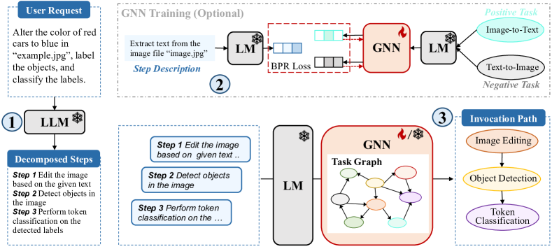
Figure 6: Illustration of our GNN-enhanced Task Planning. We first prompt LLM to decompose complex and implicit user request into several manageable sub-tasks. We then use either a training-free or training-required GNN to sequentially align each step description with a suitable task, ultimately generating the invocation path.

We compare the performance across three training-free methods: (1) LLM’s Direct Inference is introduced in Section 4.1. (2) GraphSearch [23, 36, 22] leverages the classic graph search method to generate the candidate nodes and use LLMs to give a score to the selection. Given a step, GreedySearch consistently selects the node with the highest score and adjacent to the previous task node; AdaptiveSearch selects the nodes with scores above a fixed threshold, adjusting the breadth of the search space in an adaptive mode; BeamSearch retains the $k$ nodes with highest scores. (3) SGC [47]: Employ a training-free SGC for task retrieval based on decomposed task steps. Illustrations of these methods are shown in Figures 5 and 6 in Appendix. Table 1 shows both the overall performance and token consumption costs.

Table 1: Comparison of Training-free Approaches: Overall Performance (Node-F1 and Link-F1 in $\%$) and Token Consumption in $\times 10^{3}$.

		TaskBench									RestBench
		HuggingFace			Multimedia			Daily Life			TMDB
LLM	Method	n-F1 $\uparrow$	l-F1 $\uparrow$	# Tok $\downarrow$	n-F1 $\uparrow$	l-F1 $\uparrow$	# Tok $\downarrow$	n-F1 $\uparrow$	l-F1 $\uparrow$	# Tok $\downarrow$	n-F1 $\uparrow$	l-F1 $\uparrow$	#Tok $\downarrow$
Baichuan2 13B	Direct	45.85	19.00	2.43	47.57	4.08	2.59	33.45	9.52	3.72	30.87	9.92	1.96
	GreedySearch	30.58	4.89	6.42	18.74	4.45	5.69	15.60	1.61	5.91	22.52	2.98	3.62
	AdaptiveSearch	39.30	10.41	10.81	33.24	9.22	11.17	34.39	12.73	16.71	30.33	10.00	8.71
	BeamSearch	41.06	9.59	24.69	32.24	9.09	21.60	36.18	13.18	23.83	30.97	7.61	9.08
	SGC	56.53	29.94	2.28	56.75	31.62	2.43	62.31	36.69	3.53	32.97	9.11	1.84
Vicuna 13B	Direct	50.46	21.27	2.50	53.57	23.19	2.64	73.70	45.80	3.82	44.66	14.01	2.02
	GreedySearch	52.94	25.73	6.23	46.99	23.11	5.55	42.98	13.33	7.18	45.22	13.69	3.42
	AdaptiveSearch	54.36	25.67	9.81	51.24	24.32	11.25	62.71	31.15	13.92	41.32	7.02	6.51
	BeamSearch	56.64	26.93	24.11	54.09	26.19	25.42	54.55	23.60	24.86	46.91	15.41	7.79
	SGC	59.62	31.98	2.31	61.78	37.60	2.43	83.33	63.77	3.82	48.79	15.99	1.89
CodeLlama 7B	Direct	58.06	29.39	2.44	59.44	30.83	2.57	84.12	62.89	3.82	65.67	41.99	1.94
	GreedySearch	58.71	31.56	5.84	62.83	38.12	5.35	82.51	63.83	7.08	65.51	42.60	3.12
	AdaptiveSearch	60.42	33.18	6.84	62.32	36.81	5.50	83.42	64.15	7.83	65.37	40.64	5.00
	BeamSearch	60.34	31.36	17.95	64.12	38.99	21.48	83.25	63.48	24.48	64.60	40.50	5.78
	SGC	63.98	39.27	2.30	67.04	45.04	2.43	87.73	70.49	3.59	66.15	42.62	1.88
Mistral 7B	Direct	60.60	30.23	2.49	69.83	39.85	2.64	84.26	53.63	3.77	62.23	22.02	1.96
	GreedySearch	65.91	38.13	6.52	58.92	34.72	6.26	75.18	49.47	8.27	60.64	23.18	4.38
	AdaptiveSearch	67.30	38.90	7.68	71.59	44.84	10.66	86.39	63.65	10.92	54.04	21.35	9.99
	BeamSearch	67.13	36.73	25.66	73.55	47.12	31.10	85.87	61.53	39.16	63.41	26.79	11.26
	SGC	67.43	42.08	2.32	74.07	49.90	2.43	87.13	66.49	3.54	64.72	25.67	1.89
CodeLlama 13B	Direct	57.55	28.88	2.45	68.57	41.79	2.59	91.20	76.07	3.88	68.91	43.74	2.02
	GreedySearch	61.67	34.02	5.95	67.98	42.04	4.95	91.50	76.56	5.54	66.67	42.16	3.81
	AdaptiveSearch	60.85	31.66	11.10	68.14	41.71	6.77	91.34	76.09	7.18	63.74	37.17	8.16
	BeamSearch	62.65	34.31	20.14	69.53	43.35	19.51	91.74	76.60	19.19	68.08	42.92	8.88
	SGC	65.51	39.44	2.31	73.32	53.28	2.43	92.96	79.57	3.64	71.40	47.55	1.90
GPT- 3.5-turbo	Direct	73.85	45.73	2.14	82.85	62.07	2.26	96.09	83.65	3.36	81.70	57.52	1.67
	GreedySearch	67.75	43.88	5.29	81.11	63.02	4.92	93.77	81.26	7.36	76.19	50.11	3.06
	AdaptiveSearch	72.18	47.55	7.47	81.86	62.71	5.71	93.79	81.41	8.53	77.57	53.65	5.89
	BeamSearch	75.51	49.62	14.22	83.57	64.50	12.91	95.66	82.72	22.05	81.24	57.98	6.42
	SGC	76.37	50.04	2.02	83.65	63.65	2.09	96.38	86.19	3.16	82.63	59.15	1.61
GPT- 4-turbo	Direct	77.60	52.18	2.19	88.29	69.38	2.28	97.36	84.58	3.37	82.56	56.67	1.75
	GreedySearch	74.75	50.44	5.78	86.81	69.80	5.52	97.36	85.78	7.37	75.34	49.95	3.73
	AdaptiveSearch	76.17	51.30	8.94	88.02	69.99	7.14	97.30	85.80	9.04	81.78	55.15	6.35
	BeamSearch	77.56	52.54	8.98	88.16	70.39	6.90	97.35	85.78	8.99	80.11	51.00	5.18
	SGC	77.79	52.20	2.03	88.54	69.83	2.10	97.35	85.76	3.16	82.27	56.37	1.62

Compared with direct inference, integrating SGC consistently improves performance, underscoring the effectiveness of the proposed method. GraphSearch-type methods rely on beam search to identify paths and employ LLMs for evaluation, where longer processing times generally lead to better outcomes. Notably, our proposed method achieves comparable or superior performance to BeamSearch while requiring $5$-$10$ times fewer tokens (Table 1) and inference time (Table 6). The case studies are provided in Appendix F.4. However, we observed only marginal improvements with GPT-4-turbo. A unique feature of GPT-4-turbo is its ability to manage ChatGPT-plugins, and it may have been specially trained on task planning datasets. In addition, the language model used for feature extraction in SGC is e5-355M, which may not be sufficiently powerful to effectively analyze GPT-4’s output. A detailed diagnostic analysis of cases involving GPT-4 is provided in Figure 11.

5.3 Performance of the Training-based Approaches

Settings: We further explore the efficacy of training-based GNNs in three TaskBench datasets. The TMDB dataset is excluded due to its limited sample size. Throughout our experiments, we trained a spectrum of GNN variants, both with and without co-training the small LM, whose role is to generate node embeddings derived from task names and descriptions. Owing to space constraints, we only show the performance of GraphSAGE in the main text, relegating a detailed comparison of all the situations to Table 8 and Table 9.

Observations: From Table 2, we observe a significant improvement in performance when employing a training-based GraphSAGE approach over the training-free method. However, the co-training of GNNs with e5-355M does not yield a marked improvement, suggesting that message passing is the crucial element for enhancing performance. Further analysis across a broad spectrum of GNNs (as shown in Table 8 and Table 9) reveals that powerful GNNs, such as GINs, perform similarly to networks perceived as less complex, like GCNs, and even underperform compared to GraphSAGE. This pattern indicates that the task’s challenge may not lie in the expressiveness of the models but rather in their ability to generalize.

Efficiency: The training cost is remarkably low because we use e5-355M [44] as the text embedding model for GNNs. If the trainable parameters are limited to the GNNs alone, training typically concludes within just 3 minutes. Furthermore, the training duration extends to only 15 minutes when GNNs are jointly trained with e5-355M model. This efficiency stands in stark contrast to the 10-20 hours required for tuning open-sourced LLMs. The details of the training time are given in Table 7.

Table 2: Performance of training-based GNN. The performance of all other GNNs are given in Table 8 and Table 9 in the Appendix.

		HuggingFace		Multimedia		Daily Life
LLM	Method	n-F1 $\uparrow$	l-F1 $\uparrow$	n-F1 $\uparrow$	l-F1 $\uparrow$	n-F1 $\uparrow$	l-F1 $\uparrow$
Baichuan2-13B	Direct	45.85	19.00	47.57	4.08	33.45	9.52
	GraphSAGE	59.32	34.36	56.15	31.60	65.18	40.49
	GraphSAGE (co-train)	59.76	35.59	57.97	33.29	63.21	38.10
Vicuna-13B	Direct	50.46	21.27	53.57	23.19	73.70	45.80
	GraphSAGE	61.86	35.68	63.71	39.88	86.07	67.63
	GraphSAGE (co-train)	62.82	37.04	65.89	42.18	84.23	65.44
CodeLlama-7B	Direct	58.06	29.39	59.44	30.83	84.12	62.89
	GraphSAGE	66.67	43.03	67.97	46.31	88.53	72.02
	GraphSAGE (co-train)	67.19	42.94	70.00	48.28	87.81	70.20
Mistral-7B	Direct	60.60	30.23	69.83	39.85	84.26	53.63
	GraphSAGE	68.12	43.09	75.51	52.94	87.51	66.57
	GraphSAGE (co-train)	67.61	43.14	76.96	55.46	87.61	66.75
CodeLlama-13B	Direct	57.55	28.88	68.57	41.79	91.20	76.07
	GraphSAGE	67.30	42.41	74.93	54.52	93.84	80.38
	GraphSAGE (co-train)	68.92	44.85	76.28	55.41	93.30	79.51
GPT-3.5-turbo	Direct	73.85	45.73	82.85	62.07	96.09	83.65
	GraphSAGE	77.90	52.68	85.29	65.80	96.43	86.26
	GraphSAGE (co-train)	77.87	53.04	85.51	66.56	96.34	86.09
GPT-4-turbo	Direct	77.60	52.18	88.29	69.38	97.36	84.58
	GraphSAGE	78.76	52.53	88.63	69.65	97.34	85.67
	GraphSAGE (co-train)	78.49	52.62	88.86	70.25	97.42	85.80

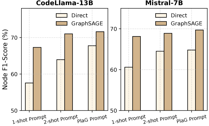
(a) Different Prompts

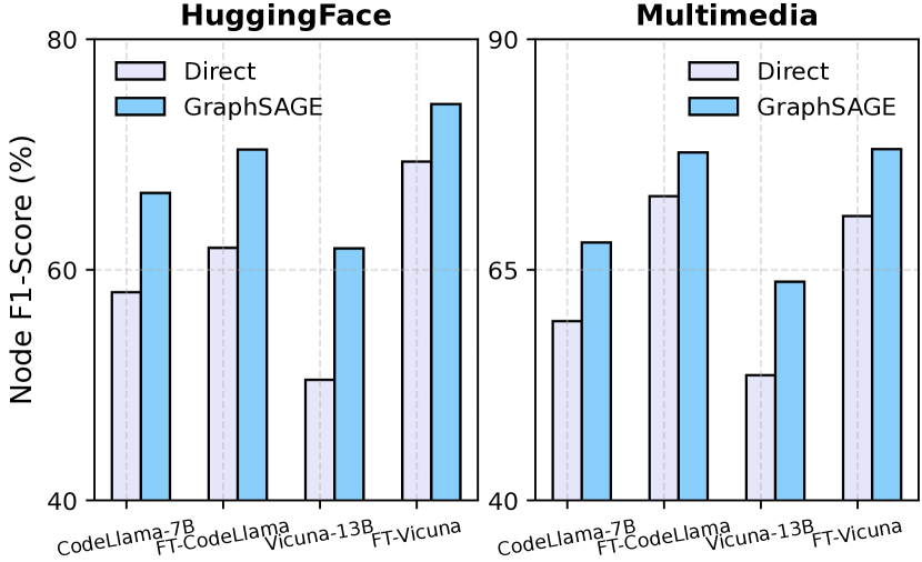
(b) Fine-tuned LLMs

Figure 3: Orthogonal Effectiveness of GNN on either different prompt templates (on HuggingFace dataset) or fine-tuned LLMs.

5.4 Improved Prompts and Fine-tuned LLMs

In this subsection, we show that the proposed method is orthogonal to two dominant methods, i.e., the prompt engineering and finetuning.

Orthogonal to Improved Prompts: We investigate GNN’s effectiveness when applied to improved prompt templates, i.e., strategically designed prompts that enhance the task planning abilities of LLMs. Specifically, we consider two types of prompts: (1) In-context Learning with Increased Examples [30] During main experiments, we maintain the consistent 1-shot in-context learning example for LLM’s direct inference. To realize further improvements, we increase the number of examples to $2$, and results under this setting are denoted as “2-shot Prompt”; (2) Plan like a Graph (PlaG) [20] We adopt the prompt in [20] to encourage LLM to think and plan in a graph-like manner, we convert the entire task graph into plain text and then integrate PlaG instructions to enhance LLM’s task planning. Results under this prompt template are denoted as “PlaG Prompt”.

From the results shown in Figure 3(a), where we apply three different prompts to CodeLlama-13B and Mistral-7B on HuggingFace, it is clear that applying a GNN to improved prompts, where task steps are more concisely decomposed and predictions are more accurate, can also boost performance.

Orthogonal to LLMs’ Fine-tuning: To explore whether our framework maintains effectiveness on fine-tuned LLMs, which have acquired dataset-specific task planning capabilities, we conduct further experiments. For each dataset, we use LoRA [13] to fine-tune two LLMs of different parameter scales, including CodeLlama-7B and Vicuna-13B, based on the same training data as GNNs. Details of fine-tuning process are provided in Appendix D.4. The finetuned model is named as “FT-CodeLlama” and “FT-Vicuna” in Figure 3(b).

The results depicted in Figure 3(b) demonstrate that fine-tuning markedly enhances the task-planning capabilities of LLMs. Furthermore, applying GraphSAGE to the decomposed tasks of LLMs further improves the accuracy of the task planning.

6 Related Works

Due to space limitations, this section focuses on related works of task planning, while discussions of other relevant areas are deferred to Appendix A. The existing studies of task planning approaches can be categorized into several directions, including task decomposition, multi-plan selection, the use of external planners, reflection, and memory-aided planning [14]. Task decomposition methods, such as the chain-of-thought approach [45], employ the divide-and-conquer strategy, utilizing LLMs for both task decomposition and sub-task planning. The application of this method to task planning is detailed in Section 4.1 and is referred to as “Direct” in the baseline comparison. Multi-plan selection strategies, exemplified by the tree-of-thought [53] and graph-of-thought [2], leverage search-based methods to generate plans. Subsequently, LLMs evaluate these plans to select the most effective one. The GraphSearch methods used in our baselines fall into this category. External planner approaches [21] formalize tasks using the Planning Domain Definition Language (PDDL) and employ classic solvers to address the planning problem, which is closely related to the proposed approaches in this paper. The task planning considered here is more flexible and cannot be directly translated into formal languages. However, we demonstrate that GNNs can serve as an effective external planner. Reflection-based methods [33] focus on reflecting upon experiences to refine the plan, while memory-aided planning approaches [55] utilize external experiences, such as those from search engines. These approaches are deployed in interactive environments and orthogonal to this paper.

7 Conclusions

This paper presents an initial exploration into graph-learning-based approaches for task planning. Through theoretical analysis, we demonstrate the inductive bias of the attention mechanism and the utility of auto-regressive loss impedes their effectiveness in task planning. We propose to integrate GNNs for task graph analysis, which yields performance improvements across a range of LLMs and datasets.

Limitations: Despite the encouraging performance, there are limitations that highlight significant opportunities for enhancement. Firstly, our proposed method, while effective, is straightforward; more sophisticated GNN-based decision-making algorithms could potentially offer further improvements. Secondly, in our current framework, GNNs function as an external module with limited interaction with LLMs. Exploring the synergies between GNNs and LLMs, particularly by incorporating GNN outputs as tokens within LLMs, presents an interesting avenue for research. Thirdly, the construction of the task graph currently requires manual effort. Investigating automated graph generation techniques for this application is another promising direction for future work.

Appendix A More Related Works

A.1 LLMs for Graphs

With the breakthroughs in LLMs, there has been a surge of interest in applying LLMs to graph-related problems. GPT4Graph [10] and NLGraph [41] are two prominent benchmarks designed to evaluate the performance of LLMs in the context of graph tasks. They encompass a wide spectrum of challenges, various input formats, and state-of-the-art prompting techniques, demonstrating that LLMs possess basic graph processing capabilities. Importantly, the choice of prompts and formats significantly influences performance. However, these benchmarks also expose the models’ susceptibility to spurious correlations within graphs. For instance, GPT-4 achieves only about $50\%$ accuracy on shortest-path tasks, even with the use of complex prompts. GraphInstruct [24] attempts to fine-tune LLMs on graph-theory-related tasks, resulting in improved performance, though it remains far from satisfactory. Despite these empirical efforts, there is a limited theoretical understanding of these evaluation results. The analysis in Section 3.2 aims to shed light on the empirical observations reported in these studies.

Considering these negative results, a new line of research has emerged that utilizes the output of GNNs as tokens for LLMs, as seen in GraphGPT [37] and GraphLLM [6]. These approaches have demonstrated significant improvements in performance on GNN-related tasks. However, they have not yet been applied to task planning due to the lack of extensive training data. A promising future direction involves using task planning data generated by GPT to fine-tune graph foundation models, such as GraphGPT [37], and applying them to task planning.

A.2 Theoretical Analysis of Reasoning

Reasoning is closely related to task planning and decision-making. The theoretical exploration of the reasoning abilities of neural networks was initiated by [50]. This work unifies various reasoning tasks, such as intuitive physics, visual question answering, and shortest path calculations, into DP problems. It then analyzes the generalization capabilities of MLPs, DeepSets, and GNNs. It is demonstrated that GNNs exhibit the best generalization bounds, attributed to their architecture’s resemblance to the Bellman-Ford algorithm, which is adept at solving DP problems. In terms of reasoning abilities within LLMs, [8] examines how the Chain of Thought (CoT) approach aids in solving arithmetic and DP problems without graphs. By decomposing challenging problems into simpler subproblems, CoT extends the expressive capabilities of Transformers from $\text{TC}^{0}$ to P. This analysis is further applied to linear and sparse Transformers in [52].

Our proof of Theorem 1 builds upon the proof of Theorem 4.7 in [8]. However, while [8] addresses DP problems without graph structures, Theorem 1 specifically focuses on DP problems with graph edge list inputs. Moreover, unlike [8], which decomposes and solves the DP problem sequentially, Theorem 1 proposes a method to simulate DP on edge lists in parallel. In addition, we analyze the negative results rising from the inductive bias of attention mechanism and auto-regressive loss. These theoretical contributions are novel and promise to be valuable for general reasoning and planning tasks.

A.3 GNNs for Decision-making

GNNs are popular approaches for solving decision-making problems on graphs. The problems investigated are typically NP-hard, such as the minimum vertex cover, maximum cut, and the traveling salesman problem [5]. The basic approach involves selecting nodes one by one in a manner that satisfies the constraints [16]. In this paper, we adopt this method to sequentially select task nodes. Furthermore, reinforcement learning can be used to enhance the performance of GNNs beyond what is achievable with supervised labels alone [16]. In [16], the node with the highest score is selected exclusively. Conversely, [19] employs beam search to improve performance by selecting the top-$k$ nodes in a single iteration. Additionally, GNNs are utilized as the method for variable selection in exhaustive searches for exact solutions to combinatorial optimization problems [9]. This paper conceptualizes task planning as a graph-based decision-making problem. Both greedy and beam search algorithms have been adopted in task planning [23, 22]. Given this connection, a promising future direction involves repurposing GNNs for decision-making approaches in task-planning applications.

Appendix B Proofs

B.1 Proof of Theorem 1

Assumption 1.

Each function $f,\oplus$ in (2) can be approximated by constant size MLP.

Assumption 2.

The aggregation function $\square$ in (2) is one of min, max, sum, mean.

The first assumption is mild as MLPs are universal approximators. The second assumption is mild because these are the most commonly used aggregation functions.

Theorem 3.

(Expressiveness) Assume the input format is given in (3) and $f,g,\square$ in DP update (2) satisfy the assumptions 1 and 2. There exists a log-precision constant-depth and constant-width Transformer that simulates $k$ steps of DP update in (2). As a consequence, there exists a log-precision $O(k)$-depth and constant-width Transformer that simulates $k$ steps of DP update in (2).

Proof.

Token Embedding and Positional Embedding: The three-dimensional token embedding includes the token type $e^{\text{type1}}$ ($0$ for answer; $1$ for node; $2$ for edge cost), refined token type $e^{\text{type2}}$ ($0$ for answer, $1$ for the node tokens in initial states, $2$ for the target node tokens in the edge list, $3$ for the source node tokens in the edge list, $4$ for edge cost), and the token id $e^{\text{token}}$ (from $0$ to $|V|-1$). The two-dimensional positional embedding includes the embedding for initial state tokens $e^{\text{pos1}}$ ($0$ for edge list tokens, $1$ for the first two elements of initial states, $2$ for the second two elements of initial states, etc.), embedding for edge list tokens $e^{\text{pos2}}$ ($0$ for initial state tokens, $1$ for the first three elements of the edge list, $2$ for the second three elements of the edge list, etc.). There are also constant-dimensional placeholders to put the states of DP.

Block 1 - Initial State Broadcast: The goal of the first block is to broadcast the initial states from the initial state token to node tokens. (1) Use MLPs to recover the digits of the answer tokens and put them in the first placeholder if $e^{type}_{k}==0$; (2) Copy the first placeholder from answer token to its previous node token by using COPY in Lemma 1 and setting $\mathcal{S}_{k}=\{j|(e^{\text{pos1}}_{k}-e^{\text{pos1}}_{j})^{2}<\delta\}$; (3) Broadcast the first placeholder with MEAN in Lemma 1 and setting $\mathcal{S}_{k}=\{j|(e^{\text{type1}}_{k}-e^{\text{type1}}_{j})^{2}+(e^{\text{token}}_{k}-e^{\text{token}}_{j})^{2}<\delta\}$. Now the state for every node token $u_{i}$ is $[e^{\text{type1}},e^{\text{type2}},e^{\text{token}},e^{\text{pos1}},e^{\text{pos2}},\text{Answer}[0][u_{i}]]$.

Block 2 - Edge Feature Operations: The goal of the second block is to copy the edge features from the edge feature token to the corresponding node tokens. (1) Use MLPs to recover the digits of the edge feature tokens and put them in the second placeholder if $e^{\text{type1}}==2$; (2) Copy the second placeholder from the edge feature token to the node token by using COPY in Lemma 1 and setting $\mathcal{S}_{k}=\{j|(e^{\text{pos2}}_{k}-e^{\text{pos2}}_{j})^{2}<\delta\}$. Now the state for every node token $u_{i}$ of the $i$-th edge is $[e^{\text{type1}},e^{\text{type2}},e^{\text{token}},e^{\text{pos1}},e^{\text{pos2}},\text{Answer}[0][u_{i}],c[u_{i}][v_{i}]]$.

Block 3 - Message Preparation: (1) Use MLPs to compute $\oplus$ and place the results in the third placeholder. Now the state for every node token $u_{i}$ of the $i$-th edge is $[e^{\text{type1}},e^{\text{type2}},e^{\text{token}},e^{\text{pos1}},e^{\text{pos2}},\text{Answer}[0][u_{i}],c[u_{i}][v_{i}],\text{Answer}[0][u_{i}]\oplus c[u_{i}][v_{i}]]$; (2) Use MLPs to clean up the first and second placeholder. Now the state for every node token $u_{i}$ is $[e^{\text{type1}},e^{\text{type2}},e^{\text{token}},e^{\text{pos1}},e^{\text{pos1}},\text{Answer}[0][u_{i}]\oplus c[u_{i}][v_{i}]]$

Block 4 - Message Passing: The goal of the fourth block is to compute $\square$ and $f$. (1) Use one or two attention heads (one for max, min, mean aggregations, and two for sum aggregations) to perform the aggregation operation. This is achieved by using MEAN or MAX or SUM for the first placeholder and setting $\mathcal{S}_{k}=\{j|(e^{\text{token}}_{k}-e^{\text{token}}_{j})^{2}+(e^{\text{type2}}_{k}-e^{\text{type2}}_{j})^{2}<\delta\}$. Now the state for every node token $u_{i}$ is $[e^{\text{type1}},e^{\text{type2}},e^{\text{token}},e^{\text{pos1}},e^{\text{pos2}},\square_{v_{j}\in\mathcal{T}(u_{i})}\text{Answer}[0][u_{i}]\oplus c[u_{i}][v_{j}]]$; (2) Use MLPs to compute $f$. Now the state for every node token is $[e^{\text{type1}},e^{\text{type2}},e^{\text{token}},e^{\text{pos1}},e^{\text{pos2}},f(\square_{v_{j}\in\mathcal{T}(i)}(\text{Answer}[0][u_{i}]\oplus c[u_{i}][v_{j}]))]$.

After four blocks, the final state for every node token $u_{i}$ is given by $[e^{\text{type1}},e^{\text{type2}},e^{\text{token}},e^{\text{pos1}},e^{\text{pos2}},\text{Answer}[1][u_{i}]]$. $\text{Answer}[k][u_{i}]$ can be obtained by repeating the above four blocks $k$ times. ∎

Lemma 1.

[8] Let $n\in\mathbb{N}$ be an integer and $\bm{x}_{1},\cdots,\bm{x}_{n}$ be a sequence of vectors where $\bm{x}_{i}=(\tilde{\bm{x}}_{i},r_{i},1)\in[-M,M]^{d+2}$ where $M$ is a large constant. Let $\bm{K},\bm{Q},\bm{V}\in\mathbb{R}^{d^{\prime}\times(d+2)}$ be any matrices with $\|\bm{V}\|_{\infty}\leq 1$ and let $0<\rho,\delta<M$ be any real numbers. Denote $\bm{q}_{i}=\bm{Q}\bm{x}_{i},\bm{k}_{j}=\bm{K}\bm{x}_{i},\bm{v}_{j}=\bm{V}\bm{x}_{j}$. Define a matching set $\mathcal{S}=\{j||\bm{q}_{i}^{T}\bm{k}_{j}|\leq\rho\}$. Define two following operations

• COPY: The output is a sequence of vectors $\bm{u}_{1},\cdots,\bm{u}_{n}$ with $\bm{u}_{i}=\bm{v}_{\text{pos}(i)}$, where $\text{pos}(i)=\arg\max_{j\in\mathcal{S}_{i}}r_{j}$.

• MEAN, MAX, SUM: The output is a sequence of vectors $\bm{u}_{1},\cdots,\bm{u}_{n}$, where $\bm{u}_{i}=\square_{j\in\mathcal{S}_{i}}\bm{v}_{j}$ and $\square$ is min or max or sum or mean.

Specifically, for any sequence of vectors $\bm{x}_{1},\bm{x}_{2},\cdots,\bm{x}_{n}$, denote the corresponding output of the attention layer as $\bm{o}_{1},\bm{o}_{2},\cdots,\bm{o}_{n}$. Then, we have $\|\bm{u}_{i}-\bm{o}_{i}\|_{\infty}\leq\epsilon$ for all $i\in[n]$ and $\mathcal{S}\neq\emptyset$.

B.2 Proof of Proposition 2

Proposition 2.

Assume the input format is as described in Equation (3) and that the attention mechanism is limited to attending to a constant number of tokens. There exists at least one instance of one-step DP update such that no log-precision constant-width constant-depth transformer can simulate.

Proof.

We present a proof by contradiction. Assume that a token in a Transformer with a constant depth, constant width, and log-precision can attend to only a constant number of nodes. Under this assumption, the total information accessible to the token in such a Transformer architecture amounts to $O(\log n)$ bits. However, for a graph with $|V|$ nodes, the number of possible outcomes from executing one-step DP is $O(e^{|V|})$, necessitating $\Theta(|V|)$ bits for representation. By the pigeonhole principle, this scenario inevitably leads to at least two distinct DP outcomes being represented by the same output sequence generated by the model, thereby constituting a contradiction. ∎

B.3 Proof of Theorem 2

Theorem 4.

(Spurious correlations of auto-regressive loss) Assume (1) the loss employed is a next-token-prediction loss utilizing cross-entropy, applied to the sub-sequence $v_{1}\ v_{2}\ \cdots\ t$ during training; (2) the output logits are determined by target node $t$ and the current node $v_{i-1}$. Let $N_{t,v_{i-1},u}$ be the number of times in the training dataset such that $t$ is the target node, $v_{i-1}$ is the current node and $v_{i}=u$ is the next node. The optimal logits for predicting the next node $u$ from current node $v_{i-1}$ towards target node $t$ is given by $\hat{\bm{v}}_{i}[u]=\frac{N_{t,v_{i-1},u}}{\sum_{u}N_{t,v_{i-1},u}}$ if $\sum_{u}N_{t,v_{i-1},u}>0$. If $\sum_{u}N_{t,v_{i-1},u}=0$, $\hat{\bm{v}}_{i}[u]$ can be any non-negative number subject to $\sum_{u}\hat{\bm{v}}_{i}[u]=1$.

Proof.

We denote $\mathcal{D}$ as the training dataset, $L_{i}$ as the sequence length of the $i$-th sequence in the dataset, $\bm{v}_{i,j}$ as the one hot embedding of the $j$-th token in the $i$-th training sequence, and $\hat{\bm{v}}_{i,j,u}$ as the $u$-th logit at the $j$-th token in the $i$-th sequence. The cross-entropy loss is given by

$$-\sum_{i\in[|\mathcal{D}|]}\sum_{j=4}^{L_{i}}\bm{v}_{i,j,u}\log\hat{\bm{v}}_{i,j,u}=-\sum_{i\in[|\mathcal{D}|]}\sum_{j=4}^{L_{i}}\mathbb{I}_{u=v_{i,j}}\log\hat{\bm{v}}_{i,j,u}\overset{(a)}{=}-\sum_{t,v_{j-1},u}N_{t,v_{j-1},u}\log\hat{\bm{v}}_{i,j,u}$$

$$\overset{(b)}{=} -\sum_{t,v_{j-1},u}\left(\sum_{u}N_{t,v_{j-1},u}\right)\left[\left(\frac{N_{t,v_{j-1},u}}{\sum_{u}N_{t,v_{j-1},u}}\right)\log\hat{\bm{v}}_{i,j,u}\right],$$

where (a) uses the assumption that the output logits are determined by target node $t$ and the current node $v_{i-1}$. In (b), we assume that $\sum_{u}N_{t,v_{i-1},u}\neq 0$. If $\sum_{u}N_{t,v_{i-1},u}=0$, then the corresponding logits will not affect the loss function and $\hat{\bm{v}}_{i,j,u}$ can take any number. The cross-entropy is minimized when $\hat{\bm{v}}_{i,j,u}=\frac{N_{t,v_{j-1},u}}{\sum_{u}N_{t,v_{j-1},u}}$. ∎

Appendix C More Discussions

C.1 Examples of Dynamic Programming

Longest Increasing Subsequence: The Longest Increasing Subsequence (LIS) problem is a classic dynamic programming problem that involves finding the length of the longest subsequence within a given array arr where the elements are in strictly increasing order. The state transition function for the LIS problem can be expressed as:

$$\text{Answer}[k][i]=\max_{j\in\mathcal{T}(i)}(\text{Answer}[k-1][j]+(\mathbb{I}(j\neq i)\times 1)),$$

where $\mathcal{T}(i)=\{i\}\cup\{j\;|j<i\;\text{and}\;\text{arr}[j]<\text{arr}[i]\}$ denotes the set of states that can transfer to state $i$, the aggregation function $\square$ is implemented as $\max(\cdot)$, and the cost $c[i][j]$ is $1$ for those candidate states that are not equal to state $i$ as adding the element leads to a longer subsequence while $0$ for the state itself.

Bellman-Ford Algorithm: The Bellman-Ford algorithm is also a classic dynamic programming algorithm used to find the shortest path from a single source vertex to all other vertices in a weighted graph. The core idea behind the Bellman-Ford algorithm is that the distance from the source vertex to a target vertex can be computed as the minimum distance from the source to any of the target’s neighboring vertices, plus the weight of the edge connecting the neighbor to the target. Therefore, the state transition function for the Bellman-Ford algorithm can be expressed as:

$$\text{Answer}[k][i]=\min_{j\in\mathcal{T}(i)}(\text{Answer}[k-1][j]+w[j][i]),$$

where $\text{Answer}[k][i]$ represents the length of the shortest path from the source vertex to node $i$ at the $k$-th iteration, $\mathcal{T}(i)=\mathcal{N}^{-}(i)$ denotes the set of in-neighbors of node $i$, and $w[j][i]$ denotes the weight from node $j$ to $i$. The aggregation function $\square$ is implemented as $\min(\cdot)$ as we try to find the shortest path.

Travelling Salesman Problem: This problem is defined as, given a set of cities and the distances between every pair of cities, finding the shortest possible route that visits every city exactly once and returns to the starting point. If we regard the set of already visited city $\mathcal{S}$ ending at $i$-th city as the current state, then states that can transfer to current state are those that ending city can reach $k$. Therefore, the state transition function for the TSP problem can be expressed as:

$$\text{Answer}[k][i][\mathcal{S}]=\min_{j\in\mathcal{S},j\neq i}(\text{Answer}[k-1][j][\mathcal{S}\setminus\{i\}]+w[j][i]),$$

where $\text{Answer}[k][i][\mathcal{S}]$ represents the cost of the shortest tour that visits all the cities in the set $\mathcal{S}$ and ends at the $i$-th city, the aggregation function is still implemented as $\min(\cdot)$ since we aim to find the shortest path, and $w[j][i]$ denotes the distance from city $j$ to city $i$.

C.2 Permutation Invariance Test of LLMs

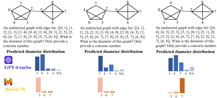
Figure 4: Illustrative Examples of LLMs Failure to Solve Graph Problems under Node-ID Permutation. Experiments were repeated for 30 times.

Appendix D Implementation Details

D.1 Details of Prompt Templates

To facilitate reproducibility, we provide prompt templates for all LLM-related queries, including direct inference and GraphSearch in Tables 3 and 4, respectively. GraphSearch consists of two types of LLM queries: Task Assessment, where LLM evaluates the suitability of each candidate task to address current step’s requirement during the iterative search, and Path Selection, where LLM selects the optimal path to fulfill user’s request after the search.

Table 3: Prompt template for LLM’s direct inference [30]

# TASK LIST # {{ task list }} # GOAL # Based on the above tasks, I want you to generate task steps and a task invocation graph (including nodes and edges) to address the # USER REQUEST #. The format must be in strict JSON format, like: $\{$ ${\color[rgb]{1,1,1}2}$ “task_steps”: $[$ step description for one or more steps $]$, ${\color[rgb]{1,1,1}2}$ “task_nodes”: $[\{$ ${\color[rgb]{1,1,1}2}\quad$ “task”: “ task name must be from # TASK LIST # ”, ${\color[rgb]{1,1,1}2}\quad$ “arguments”: $[$ a concise list of arguments for the task $]$ ${\color[rgb]{1,1,1}2}$$\}]$, ${\color[rgb]{1,1,1}2}$ “task_links”: $[\{$ “source”: “task name i”, “target”: “task name j” $\}]$, $\}$ # REQUIREMENTS # 1. Generated task steps and task nodes can resolve the user request # USER REQUEST # perfectly. Task name must be selected from # TASK LIST #. 2. The task steps should strictly align with the task nodes, and the number of task steps should be same with the task nodes. 3. The task links should reflect the temporal and resource dependencies among task nodes, i.e., the order in which the tasks are invoked. # EXAMPLE # {{ in-context learning examples }} # USER REQUEST # {{ user request }} Now, please generate your response in a strict JSON format: # RESULT #

Table 4: Prompt templates of GraphSearch [23]

Scenario	Prompt
Task Assessment	# CANDIDATE TASK LIST # {{ candidate tasks }} # GOAL # Based on the provided # CANDIDATE TASK LIST # and the user’s request described in the # STEP #, generate a score dictionary to assess each task’s problem-solving abilities. The output must be in a strict JSON format, like: $\{$ “candidate task name 1”: score, … $\}$. # REQUIREMENTS # 1. The keys of the generated score dictionary must align with the provided candidate tasks, and you should output scores for all candidate tasks. 2. The “score” field denotes a concrete score that assesses whether each task can solve the given step’s demand. The score should be in the range of $[1,2,3,4,5]$, where a higher score indicates better task-solving and matching abilities. 3. Carefully consider the user’s intention in # STEP # to assign the score. If the # STEP # contains a candidate task, its score should be >= 3. # EXAMPLE # {{ in-context learning examples }} # STEP # {{ step description }} Now please generate your result in a strict JSON format: # RESULT #
Path Selection	# GOAL # Based on the provided # USER REQUEST # and initially inferred # STEPS #, select the best path solution list from # SOLUTION LIST #. The selected solution should be the one that can perfectly solve the user’s request and strictly align with the inferred steps. The output must be in strict JSON format, like: $\{$ “best_solution”: $[$list of invoked tasks $]\}$ # REQUIREMENTS # 1. Carefully analyze both the user’s request and previously inferred task steps. Select the best solution that can perfectly follow the inferred steps and solve user’s request. Do not change their corresponding sequences. 2. Make sure that each task in the final solution list exists in the valid # TASK LIST # {{ task list }}. # USER REQUEST # {{ user request }} # STEPS # {{ steps }} # SOLUTION LIST # {{ list of searched solutions }} Now please generate your result in a strict JSON format: # RESULT #

D.2 Implementation of Training-free Methods

In this subsection, we present the implementation details of two training-free baselines, including LLM’s direct inference and GraphSearch. Method illustrations are shown in Figure 5.

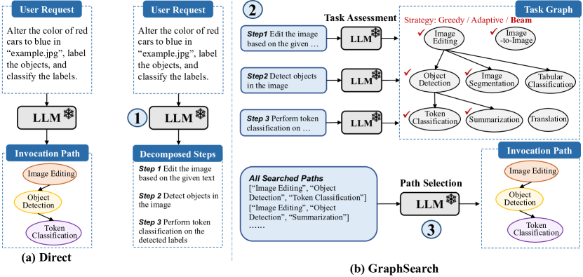
Figure 5: Illustration of LLM’s Direct Inference and GraphSearch Method.

LLM’s Direct Inference: During experiments, we uniformly apply 1-shot in context learning for LLM’s direct inference of task invocation path. For open-sourced LLMs, the temperature parameter is set to 0.2.

GraphSearch: This algorithm conducts an iterative search on the task graph to identify an optimal task invocation path that can best satisfy a given request. In each iteration, the neighbors of the last selected task are considered as candidates. These candidates are evaluated by LLM for their suitability for the current step. The search process follows a depth-first approach. After the task assessment in the final step, a set of potential invocation paths is generated. Subsequently, LLM is prompted to select the most appropriate path from these options. The GraphSearch algorithm is implemented in three distinct variants, each employing a unique task selection strategy:

• GreedySearch consistently selects the task node with the highest score at each step. Although fast and simple, this approach can lead to cascading errors, resulting in degraded performance.

• AdaptiveSearch selects tasks with scores above a fixed threshold, adjusting the breadth of the search space in an adaptive mode. During experiments, we empirically set the score threshold to 3.

• BeamSearch retains the top-$k$ tasks based on the LLM’s assessment scores within candidates. Beam search can expand the search space but slightly reduces the efficiency. We uniformly set the beam width to 2.

SGC: For the implementation of SGC, the parameter $\alpha$ is uniformly set to 0.7. Regarding the choices of LM backbones, for integrating GPT-3.5-turbo and GPT-4-turbo with SGC on HuggingFace dataset, Roberta-large-355M [26] serves as the text encoder. For all other datasets and LLMs, the e5-355M [44] configuration is employed.

D.3 Implementation of Training-based GNNs

LM and GNN Configuration: For training-based GNNs, we uniformly use the e5-355M [44] as the LM backbone. For the graph encoder, our setup includes a single layer with a hidden dimension of 1024. During the model training, we set the batch size to 512 and run for 20 epochs with a learning rate of 1e-3. We use the Adam optimizer [17] and implement an early stopping mechanism with a patience of 5 epochs to prevent over-fitting. All experiments are conducted on a single NVIDIA A100-80G GPU.

Training Data Preparation: From each dataset in TaskBench, we randomly select $3,000$ samples to create the trainset. The original data includes specific task steps and corresponding task invocation paths. Therefore, we first employ a topological sort to align each task step accurately with corresponding task, forming “<step, ground-truth task>” pairs. Then, for each pair, we randomly sample 2 negative tasks to constitute the “<step, positive task, negative task>” triplets for model training. These negative samples are selected based on how textually similar they are to the positive one, creating a robust differentiation challenge for the model.

Choices of Different Configurations: Our training-based method offers two configuration options: training only the GNN while keeping the LM frozen, or co-training both the LM and GNN. The first configuration is designed to explore GNN’s capability in task retrieval. The latter leverages LM’s dataset-specific semantic embeddings to enhance performance. Illustrations of these configurations are provided in Figure 7. For the co-training setup, we use a learning rate of 2e-5 and a training duration of 10 epochs.

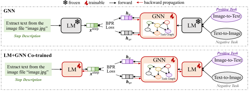
Figure 7: LM+GNN Configuration. We offer two configurations: only training the GNN while keeping the LM frozen (Table 8), or co-training both the LM and GNN (Table 9).

D.4 Fine-tuning LLMs

To explore the effectiveness of our proposed framework on fine-tuned LLMs, we employ Supervised Fine-Tuning (SFT) on the CodeLlama-7B and Vicuna-13B models. We use the same set of $3,000$ samples from GNN training as the LLMs’ fine-tuning data. In fine-tuning the LLM with LoRA [13], we set the lora_r parameter (dimension for LoRA update matrices) to 8 and the lora_alpha (scaling factor) to 16. The dropout ratio is set to 0.1, the batch size to 2, and we conduct training over 2 epochs with a learning rate of 1e-5. For HuggingFace dataset, the maximum input length is set to 800, while the maximum output length is 400. For Multimedia and Daily Life datasets, which contain a larger number of tasks and require longer textual inputs, we set the maximum input and output length to 1000 and 500, respectively. We utilize 2 NVIDIA A100-80G GPUs for fine-tuning the LLMs. Each dataset undergoes specific fine-tuning for both the CodeLlama-7B and Vicuna-13B models.

Appendix E Datasets

E.1 Overview

We provide the statistics of experimental datasets from two task planning benchmarks in Table 5. The illustrative examples from each dataset are shown in Figure 8. For datasets from TaskBench, each sample consists of original user request, corresponding decomposed task steps, and ground-truth task invocation path. As RestBench includes only user requests and corresponding API invocation sequences, we prompt GPT-4 to infer decomposed task steps aligned with each invoked API, thereby finalizing the dataset.

E.2 Reformatting Details of RestBench

The TMDB dataset from RestBench, focuses on movie-related searching and recommending functions. To align RestBench with our experiments, we have implemented the following processing steps: Reformatting original APIs by assigning unique task names and descriptions: APIs in RestBench were represented by request paths, such as “GET /movie/top_rated”, referring to the API that retrieves top-rated movies on TMDB. To enhance semantic differentiation among APIs, we first prompt GPT-4 to assign a unique name and a detailed functional description to each API. These names and descriptions were then manually verified and refined. For example, the API previously mentioned is renamed “Get Top-Rated Movies” with the description “This API retrieves a list of the highest-rated movies.” Note that though the original TMDB dataset contains 54 APIs, some were never invoked in any data examples. Therefore, we focus only on those APIs that appeared in at least one user request, resulting in a refined set of 46 APIs.

Constructing a Task Graph: Each API is regarded as a unique task node, and we depict their relationships from two aspects: (1) categorical association, and (2) resource dependencies. For instance, APIs that provide movie-related functionalities, such as retrieving movie details or recommending films, are grouped under the movie category. Conversely, APIs focused on person-related functions, like searching for actors, are classified under the person category. Additionally, if two APIs share a common parameter like move_id, we establish a link between them to indicate a resource dependency.

Reformatting Raw Data Examples: The original data samples in RestBench included a single query and its corresponding API invocation sequence. To reformat this data into a path structure, we treated each invoked API as a node and the sequence of invocations as directed links from one API to the next. For example, a TMDB data sample consists of the query “Who was the lead actor in the movie The Dark Knight” and corresponding ground-truth API solution $[$“GET /search/movie”, “GET /movie/{movie_id}/credits”$]$. We transform this solution into a task invocation path as “$\{$ “task_nodes”: $[$“Search Movie”, “Get Movie Credit”$]$, “task_links”: $[\{$“source”: “Search Movie”, “target”: “Get Movie Credit”$\}]\}$ ”.

Table 5: Statistics of Experimental Datasets

		TaskBench			RestBench
Type	Statistic	HuggingFace	Multimedia	Daily Life	TMDB
Task Graph	# Nodes	23	40	40	46
	# Links	225	449	1560	979
	Link Type	Resource	Resource	Temporal	Resource / Category
All Data	# Samples	7,546	5,584	4,320	100
Test Set	# Samples	500	500	500	94
	# Avg. Nodes	3.81	3.92	4.05	2.33
	# Avg. Links	2.81	2.92	3.05	1.33

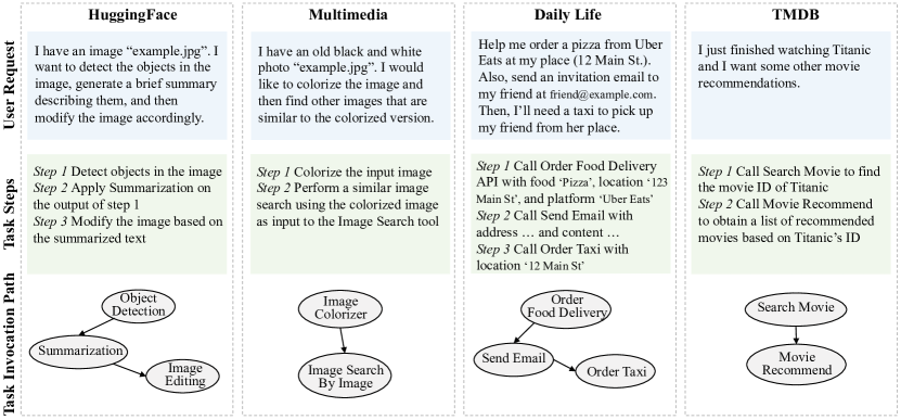
Figure 8: Illustrative examples of four experimental datasets.

Appendix F Supplementary Experiments

F.1 Full Results of Training-based GNNs

In Table 8, we present comprehensive results for all training-based GNNs, including GCN [18], GAT [39], GraphSAGE [11], GIN [49], and TransformerConv [32]. To highlight the improvements brought by GNNs, we also include results from the strongest baseline, BeamSearch.

From the results, it is obvious that all GNN encoders significantly enhance the task planning abilities. For instance, when applied to Vicuna-13B on HuggingFace dataset, the introduction of GCN results in a performance improvement of $17.83\%$, GAT contributes to a $17.48\%$ increase, GraphSAGE leads to a $22.59\%$ boost, and TransformerConv improves predictions by $18.0\%$. This conclusion can be generalized across various LLMs and datasets, demonstrating the robust capabilities of GNNs.

F.2 Performance of LM+GNN Co-trained Mode

In this subsection, we conduct a supplementary study where the parameters of a pre-trained LM are also tuned along with GNN during model training. The model configuration is illustrated in Figure 7, and the results are presented in Table 9.

The results demonstrate that, compared to the GNN-only tunable mode, co-training LM+GNN can lead to further performance improvements. This enhancement occurs because the language model acquires task-specific semantics, which makes the representations more discriminative and boosts the GNN’s effectiveness in task retrieval. Additionally, it is noted that under the co-training setup, the differences between various GNN encoders are relatively minor, with performance variations across GNNs for a specific LLM on any dataset remaining within $2\%$.

For LM+GNN co-trained mode, as the parameters of the LM backbone, e5-355M, are also trained, more computational resources are required. We list the number of trainable parameters and the required training times for this architecture in Table 7. In application scenarios, the choice between GNN-only and LM+GNN co-trained modes can be decided based on the availability of resources and performance requirements.

F.3 Full Efficiency Study

In this subsection, we present a comprehensive efficiency study on various experimental setups: inference times across different training-free modes, time required for training GNN or LM+GNN, and the resources needed for fine-tuning LLMs. Results are shown in Tables 6 and 7.

Table 6: Efficiency Study of Training-free Methods. Due to space constraints in the table, some LLMs are abbreviated such as “GPT-3.5” for “GPT-3.5-turbo”. For Vicuna-13B and Mistral-7B, some discrepancies in reported times may be attributed to variations in deployment across different A100 devices. SGC maintains efficiency comparable to LLM’s direct inference.

	Inference Times Comparison on HuggingFace (Seconds)
Mode	Baichuan	Vicuna	CodeLlama-7B	Mistral	CodeLlama-13B	GPT-3.5	GPT-4
Direct	6.0	3.6	10.9	4.5	9.7	2.7	26.1
GreedySearch	30.7	45.7	23.1	109.8	29.1	7.4	55.6
AdaptiveSearch	50.2	79.4	27.2	28.2	52.4	9.4	87.0
BeamSearch	102.0	55.0	60.8	85.5	92.3	14.9	270.2
SGC	6.1	3.7	10.7	4.6	9.5	3.0	24.4
	Inference Times Comparison on Multimedia (Seconds)
Direct	9.7	3.3	13.2	4.5	14.6	2.9	25.1
GreedySearch	52.3	54.3	37.0	109.7	9.9	8.8	52.2
AdaptiveSearch	98.1	142.5	25.7	41.6	25.6	9.6	84.2
BeamSearch	122.3	69.8	103.0	92.0	84.4	15.0	70.9
SGC	9.5	3.4	12.9	4.5	14.1	3.1	23.5
	Inference Times Comparison on Daily Life (Seconds)
Direct	10.0	6.5	19.4	5.6	18.6	3.4	31.0
GreedySearch	62.7	49.8	29.3	198.3	37.6	13.2	124.3
AdaptiveSearch	133.3	97.6	30.5	69.1	45.5	16.5	209.0
BeamSearch	196.9	54.1	106.9	195.9	64.9	89.4	161.7
SGC	9.9	6.5	18.6	5.7	17.9	3.6	29.5

Table 7: Efficiency Study of Training-based Methods. We present total training times for both GNN and LM+GNN co-trained modes, and resources needed for fine-tuning LLMs.

Training GNNs
			Time (Seconds)
Mode	Configuration	# Param	HuggingFace	Multimedia	Daily Life
GNN-only	GCN	1,049,600	136.5	136.1	237.7
	GAT	1,051,648	136.9	151.8	237.8
	GraphSAGE	2,098,176	134.2	149.8	233.8
	GIN	2,099,200	134.2	134.9	233.6
	TransformerConv	4,198,400	135.0	150.2	233.7
LM+GNN Co-trained	LM+SGC	335,141,889	743.1	323.3	384.7
	LM+GCN	336,191,488	482.8	567.8	384.2
	LM+GAT	336,193,536	741.3	812.3	384.4
	LM+GraphSAGE	337,240,064	741.2	406.8	381.7
	LM+GIN	337,241,088	735.6	361.8	382.9
	LM+TransformerConv	339,340,288	741.0	362.7	405.8

Fine-tuning LLMs
		Device & Time (Hours)
LLM	# Param (# Tunable Param)	HugggingFace	Multimedia	Daily Life
CodeLlama-7B	6,742,740,992 (4,194,304)	2$\times$A100 7.0	1$\times$A100 13.8	2$\times$A100 9.5
Vicuna-13B	13,022,417,920 (6,553,600)	1$\times$A100 17.8	2$\times$A100 10.3	2$\times$A100 19.0

Efficiency of Training-free Modes: Open-sourced LLMs were deployed as local API services using the FastChat framework on a single A100-80G GPU. This configuration enables faster and parallel inference. Under this setup, LLM’s direct inference requires 3-15 seconds per request. GPT-3.5-turbo and GPT-4-turbo are accessed via API, with the latter generally requiring more time. GraphSearch requires several minutes to complete a request due to its exhaustive search on the task graph, impacting the efficiency. In contrast, SGC achieves comparable efficiency to LLM’s direct inference, as it requires only a single LLM query and both LM and SGC’s forward propagation processes are extremely efficient. Note that some discrepancies in reported times, such as Mistral-7B’s GreedySearch taking longer than other modes, may be attributed to variations in the deployment across different A100 GPUs.

Efficiency of Training GNNs: During experiments, each dataset shares the same GNN configuration: 1 single layer with a hidden dimension of 1024. Therefore, for each GNN, the number of parameters remains consistent across datasets. The parameter scales for GNN variants range from 1M to 4M, and the total training time for each dataset requires only 2-4 minutes, comparable to the time taken by GraphSearch to fulfill a single request. For LM+GNN co-trained mode, where e5-355M serves as the LM backbone, training times increase to approximately 6-12 minutes. In summary, both modes demonstrate high efficiency, with total training times spanning minutes, showcasing their ability to rapidly adapt to new task planning scenarios.

Efficiency of Fine-tuning LLMs: Fine-tuning a LLM with $3,000$ training samples over 2 epochs requires huge time, typically 10-20 hours on one or two A100-80G GPU devices.

F.4 Case Study

Effectiveness of GNN (Qualitative Result): We show two cases in Figure 9 where the results of LLM’s direct inference, BeamSearch, and GraphSAGE are compared. Due to space constraints and issues such as LLM’s output content decoding errors or invalid paths, we present only the first four valid paths searched by BeamSearch on the task graph. From the cases, we can conclude that BeamSearch relies on LLM’s inherent reasoning abilities. Although LLM can explore the ground-truth invocation path on the task graph, their final solutions are usually not the optimal as containing either the hallucination or wrongly invoked tasks due to limited instruction following and reasoning abilities. On the contrary, GNN can effectively align decomposed steps with suitable tasks, accurately hitting the ground-truth result and enhancing task planning.

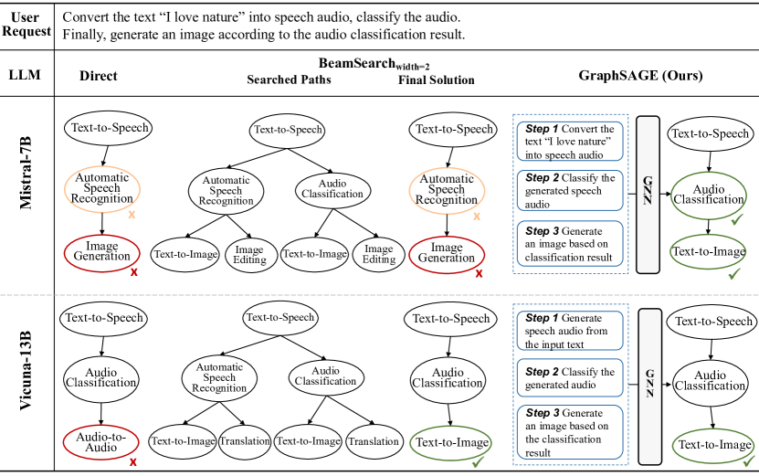
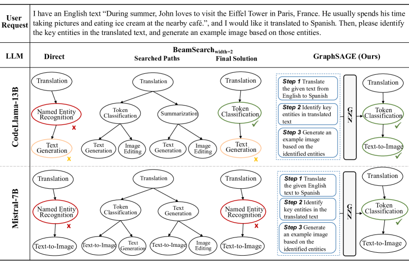
Figure 9: Case Study of GNN’s Effectiveness. Nodes colored in pink and red denote wrongly predicted task or hallucinated task, respectively. Due to space limitations, we only show the first four valid searched paths of BeamSearch for illustration. Even though LLM can explore ground-truth paths during searching, they lack certain instruction-following and reasoning abilities to consistently choose the optimal path. On the contrary, GNN can correctly align decomposed steps with suitable tasks, hitting the ground-truth result.

Failure Cases of GNNs: We also present the failure cases where GNN performance deteriorates compared to direct inference to provide a comprehensive discussion of our method. Our conclusion is that the method is sensitive to the quality of decomposed task steps, as an ambiguous step may mislead GNN to wrongly select the task, and such errors can cascade due to the sequential selection of tasks on the task graph. As the case shown in Figure 10, step 2 is ambiguously described as “Segment the image and identify the tabular data”, which actually incorporates two distinct steps. This ambiguty causes GNN to choose the unsuitable Tabular Classification instead of the correct Image Segmentation. Since tasks are selected sequentially on the task graph, where the next task is a neighbor of the current selection, such an error can prevent the exploration of the next appropriate task, as it may not be a neighbor of the current, incorrect selection. We also present the BeamSearch explored paths and its final solution, where it hits the ground-truth result.

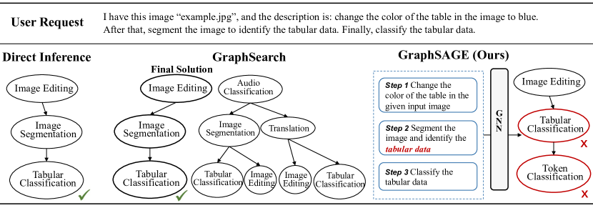
Figure 10: Failure cases of GNN. Our framework relies heavily on the quality of decomposed task steps. Ambiguous steps (step 2 actually incorporates two steps) may mislead GNN to select the wrong task.

Diagnosing GraphSearch with GPT-4-turbo: In our experiments, GraphSearch brings marginal or even decreased performance for GPT-4-turbo across most experimental datasets, contradicting current research [23, 22] which suggests that exhaustive search strategies can enhance the performance of more powerful LLMs. To provide a detailed analysis, we show three types of cases in Figure 11: Successful cases, Failure cases, as well as Maintaining cases:

• Successful Cases: As shown in the figure, despite inaccuracies in task decomposition (GPT-4-turbo predicts an extra step compared to the three-step ground truth), its inherent reasoning abilities and the knowledge explored along the task graph can fix these mistakes, hitting the ground-truth.

• Failure Cases: In the failure case, although GPT-4-turbo identifies the ground-truth solution during searching process, the final decision includes an incorrect task. This occurs because the final solution selection demands complex reasoning abilities of LLM, as the context contains long textual information from different aspects: the full task graph, user request, all searched paths, and related instructions (Prompt template is shown in Table 4). The demanding context and reasoning challenge exceed GPT-4’s capabilities, leading to errors.

• Maintaining Cases: These occur when GraphSearch merely replicates the result of GPT-4-turbo’s direct inference, indicating no added benefit from exploring the task graph. In these instances, despite navigating the graph, GPT-4 fails to self-correct inaccuracies due to inherent reasoning limitations.

We emphasize that the results of GraphSearch with GPT-4-turbo, tend to “maintaining cases”. Under such conditions, even a few failures can degrade overall performance, explaining why GraphSearch does not consistently enhance performance for GPT-4-turbo.

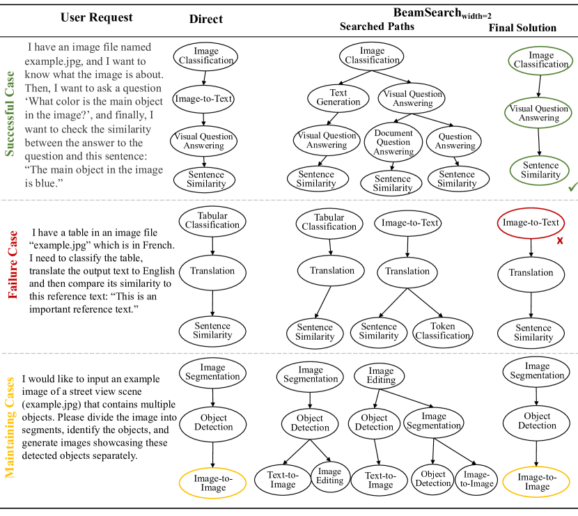
Figure 11: Diagnosing GraphSearch with GPT-4-turbo. We provide three types of cases: (1) Successful Cases where GPT-4 can leverage inherent reasoning abilities to select the optimal invocation path. (2) Failure Cases where GPT-4 miss in the extremely long context, containing the whole task graph, all searched paths, and instructions, selecting an unsatisfactory path. (3) Maintaining Cases where the searched result is the same as direct inference result, and those wrongly predicted tasks can still not be refined even under exhaustive search.

Table 8: Performance of training-based GNNs. We also presents the results of BeamSeaerch, the strongest variant from GraphSearch method to provide a comprehensive comparison. All GNNs consistently enhance task planning performance across diverse LLMs, showing the effectiveness.

		HuggingFace Tools		Multimedia Tools		Daily Life APIs
LLM	Method	n-F1 $\uparrow$	l-F1 $\uparrow$	n-F1 $\uparrow$	l-F1 $\uparrow$	n-F1 $\uparrow$	l-F1 $\uparrow$
Baichuan2-13B	Direct	45.85	19.00	47.57	4.08	33.45	9.52
	BeamSearch	41.06	9.59	32.24	9.09	36.18	13.18
	GCN	57.67	31.47	55.51	30.16	62.11	37.05
	GAT	57.74	31.87	54.95	29.24	62.11	37.05
	GraphSAGE	59.32	34.36	56.15	31.60	65.18	40.49
	GIN	57.38	31.17	55.08	30.04	62.11	37.05
	TransformerConv	59.15	34.36	56.06	31.12	64.52	40.14
Vicuna-13B	Direct	50.46	21.27	53.57	23.19	73.70	45.80
	BeamSearch	56.64	26.93	54.09	26.19	54.55	23.60
	GCN	59.46	33.14	62.48	38.89	83.05	62.95
	GAT	59.28	33.39	62.96	39.24	83.05	62.95
	GraphSAGE	61.86	35.68	63.71	39.88	86.07	67.63
	GIN	59.14	32.33	62.61	38.82	83.05	62.95
	TransformerConv	59.57	33.47	63.32	39.38	85.41	66.28
CodeLlama-7B	Direct	58.06	29.39	59.44	30.83	84.12	62.89
	BeamSearch	60.34	31.36	64.12	38.99	83.25	63.48
	GCN	65.07	40.50	67.46	45.84	87.23	69.27
	GAT	65.20	40.93	67.41	46.46	87.23	69.27
	GraphSAGE	66.67	43.03	67.97	46.31	88.53	72.02
	GIN	65.52	40.98	66.89	45.41	87.23	69.27
	TransformerConv	65.83	42.58	68.90	47.20	88.36	71.72
Mistral-7B	Direct	60.60	30.23	69.83	39.85	84.26	53.63
	BeamSearch	67.13	36.73	73.55	47.12	85.87	61.53
	GCN	66.54	40.74	73.34	50.76	86.39	65.49
	GAT	66.77	40.74	73.36	50.20	86.39	65.49
	GraphSAGE	68.12	43.09	75.51	52.94	87.51	66.57
	GIN	66.69	40.79	72.89	50.44	86.39	65.49
	TransformerConv	68.26	43.08	73.80	51.45	88.25	67.84
	Direct	57.55	28.88	68.57	41.79	91.20	76.07
	BeamSearch	62.65	34.31	69.53	43.35	91.74	76.60
	GCN	66.22	41.05	72.99	52.18	91.83	77.88
	GAT	66.29	41.28	74.08	53.56	91.83	77.88
	GraphSAGE	67.30	42.41	74.93	54.52	93.84	80.38
	GIN	66.40	40.89	73.62	53.15	91.83	77.88
CodeLlama-13B	TransformerConv	66.70	42.07	74.72	54.10	93.81	80.44
GPT-3.5-turbo	Direct	73.85	45.73	82.85	62.07	96.09	83.65
	BeamSearch	75.51	49.62	83.57	64.50	95.66	82.72
	GCN	76.93	51.43	84.92	65.05	96.38	86.15
	GAT	75.63	49.36	84.77	65.48	96.38	86.15
	GraphSAGE	77.90	52.68	85.29	65.80	96.43	86.26
	GIN	76.86	51.00	84.14	64.30	96.38	86.15
	TransformerConv	77.61	52.30	84.21	64.32	96.38	86.19
GPT-4-turbo	Direct	77.60	52.18	88.29	69.38	97.36	84.58
	BeamSearch	77.56	52.54	88.16	70.39	97.35	85.78
	GCN	77.01	50.49	88.56	69.60	97.10	85.22
	GAT	76.41	49.66	88.43	69.52	97.10	85.22
	GraphSAGE	78.76	52.53	88.63	69.65	97.34	85.67
	GIN	77.74	51.02	88.05	69.13	97.36	84.58
	TransformerConv	78.47	52.17	88.07	68.71	97.32	85.57

Table 9: Performance of Training-based GNNs under the LM+GNN Co-trained Mode. Simultaneous training of LM and GNN yields significant performance improvements.

		HuggingFace Tools		Multimedia Tools		Daily Life APIs
LLM	Method	n-F1 $\uparrow$	l-F1 $\uparrow$	n-F1 $\uparrow$	l-F1 $\uparrow$	n-F1 $\uparrow$	l-F1 $\uparrow$
Baichuan2-13B	Direct	45.85	19.00	47.57	4.08	33.45	9.52
	SGC	60.97	36.12	56.02	31.36	64.84	40.00
	GCN	60.68	36.31	57.82	32.87	64.73	38.92
	GAT	60.39	35.37	57.24	32.19	64.46	40.14
	GraphSAGE	59.76	35.59	57.97	33.29	63.21	38.10
	GIN	60.31	35.82	56.62	31.53	63.55	38.19
	TransformerConv	60.76	36.82	56.82	31.40	64.88	40.23
Vicuna-13B	Direct	50.46	21.27	53.57	23.19	73.70	45.80
	SGC	64.40	38.97	65.12	41.63	84.74	65.90
	GCN	62.06	35.49	65.02	40.63	85.22	66.93
	GAT	63.06	36.97	64.58	40.30	85.63	67.11
	GraphSAGE	62.82	37.04	65.89	42.18	84.23	65.44
	GIN	62.09	35.33	64.44	40.67	85.31	66.83
	TransformerConv	62.11	36.01	64.57	40.17	85.42	66.55
CodeLlama-7B	Direct	58.06	29.39	59.44	30.83	84.12	62.89
	SGC	67.47	43.58	69.61	48.24	87.98	70.63
	GCN	67.03	43.24	69.33	47.60	87.88	70.40
	GAT	67.12	42.96	68.62	46.17	88.59	71.64
	GraphSAGE	67.19	42.94	70.00	48.28	87.81	70.20
	GIN	66.62	42.34	69.00	47.72	88.45	71.53
	TransformerConv	67.12	43.08	69.27	47.96	88.43	71.59
Mistral-7B	Direct	60.60	30.23	69.83	39.85	84.26	53.63
	SGC	69.04	44.22	76.09	54.91	87.58	66.70
	GCN	67.72	43.02	76.79	54.90	87.87	67.13
	GAT	67.54	43.56	76.26	53.94	87.86	67.30
	GraphSAGE	67.61	43.14	76.96	55.46	87.61	66.75
	GIN	68.95	43.97	76.47	54.95	87.75	67.07
	TransformerConv	67.94	43.52	77.06	55.39	87.76	67.00
CodeLlama-13B	Direct	57.55	28.88	68.57	41.79	91.20	76.07
	SGC	70.14	45.20	75.65	55.45	93.45	79.89
	GCN	69.39	45.18	76.03	55.22	93.38	79.74
	GAT	69.68	45.57	75.24	54.99	94.06	80.96
	GraphSAGE	68.92	44.85	76.28	55.41	93.30	79.51
	GIN	69.01	44.76	74.72	53.91	94.24	81.23
	TransformerConv	69.52	45.68	75.46	55.14	93.98	81.06
GPT-3.5-turbo	Direct	73.85	45.73	82.85	62.07	96.09	83.65
	SGC	77.87	52.86	85.95	66.95	96.39	86.16
	GCN	77.72	52.58	85.84	66.92	96.33	86.06
	GAT	77.49	52.30	85.81	66.97	96.38	86.15
	GraphSAGE	77.87	53.04	85.51	66.56	96.34	86.09
	GIN	77.73	52.36	85.63	66.69	96.38	86.19
	TransformerConv	77.78	52.79	86.09	67.26	96.33	86.06
GPT-4-turbo	Direct	77.60	52.18	88.29	69.38	97.36	84.58
	SGC	78.44	52.84	89.09	70.52	97.38	85.85
	GCN	78.33	52.75	89.00	70.24	97.34	85.67
	GAT	78.37	52.43	88.99	70.48	97.32	85.56
	GraphSAGE	78.49	52.62	88.86	70.25	97.42	85.80
	GIN	78.45	53.07	88.74	69.84	97.42	85.80
	TransformerConv	78.30	52.27	88.90	70.24	97.42	85.80

References

- Bellman [1966] Richard Bellman. Dynamic programming. Science, 153(3731):34–37, 1966.
- Besta et al. [2024] Maciej Besta, Nils Blach, Ales Kubicek, Robert Gerstenberger, Michal Podstawski, Lukas Gianinazzi, Joanna Gajda, Tomasz Lehmann, Hubert Niewiadomski, Piotr Nyczyk, et al. Graph of thoughts: Solving elaborate problems with large language models. In Proceedings of the AAAI Conference on Artificial Intelligence, volume 38, pp. 17682–17690, 2024.
- Boiko et al. [2023] Daniil A Boiko, Robert MacKnight, Ben Kline, and Gabe Gomes. Autonomous chemical research with large language models. Nature, 624(7992):570–578, 2023.
- Bubeck et al. [2023] Sébastien Bubeck, Varun Chandrasekaran, Ronen Eldan, Johannes Gehrke, Eric Horvitz, Ece Kamar, Peter Lee, Yin Tat Lee, Yuanzhi Li, Scott Lundberg, et al. Sparks of artificial general intelligence: Early experiments with GPT-4. arXiv preprint arXiv:2303.12712, 2023.
- Cappart et al. [2023] Quentin Cappart, Didier Chételat, Elias B Khalil, Andrea Lodi, Christopher Morris, and Petar Veličković. Combinatorial optimization and reasoning with graph neural networks. Journal of Machine Learning Research, 24(130):1–61, 2023.
- Chai et al. [2023] Ziwei Chai, Tianjie Zhang, Liang Wu, Kaiqiao Han, Xiaohai Hu, Xuanwen Huang, and Yang Yang. GraphLLM: Boosting graph reasoning ability of large language model. arXiv preprint arXiv:2310.05845, 2023.
- Dudzik & Veličković [2022] Andrew J Dudzik and Petar Veličković. Graph neural networks are dynamic programmers. Advances in neural information processing systems, 35:20635–20647, 2022.
- Feng et al. [2024] Guhao Feng, Bohang Zhang, Yuntian Gu, Haotian Ye, Di He, and Liwei Wang. Towards revealing the mystery behind chain of thought: a theoretical perspective. Advances in Neural Information Processing Systems, 36, 2024.
- Gasse et al. [2019] Maxime Gasse, Didier Chételat, Nicola Ferroni, Laurent Charlin, and Andrea Lodi. Exact combinatorial optimization with graph convolutional neural networks. Advances in neural information processing systems, 32, 2019.
- Guo et al. [2023] Jiayan Guo, Lun Du, and Hengyu Liu. Gpt4graph: Can large language models understand graph structured data? an empirical evaluation and benchmarking. arXiv preprint arXiv:2305.15066, 2023.
- Hamilton et al. [2017] William L. Hamilton, Rex Ying, and Jure Leskovec. Inductive representation learning on large graphs. In NIPS, 2017.
- He et al. [2020] Xiangnan He, Kuan Deng, Xiang Wang, Yan Li, Yongdong Zhang, and Meng Wang. LightGCN: Simplifying and powering graph convolution network for recommendation. In Proceedings of the 43rd International ACM SIGIR conference on research and development in Information Retrieval, pp. 639–648, 2020.
- Hu et al. [2021] J. Edward Hu, Yelong Shen, Phillip Wallis, Zeyuan Allen-Zhu, Yuanzhi Li, Shean Wang, and Weizhu Chen. Lora: Low-rank adaptation of large language models. ArXiv, abs/2106.09685, 2021.
- Huang et al. [2024] Xu Huang, Weiwen Liu, Xiaolong Chen, Xingmei Wang, Hao Wang, Defu Lian, Yasheng Wang, Ruiming Tang, and Enhong Chen. Understanding the planning of LLM agents: A survey. arXiv preprint arXiv:2402.02716, 2024.
- Jiang et al. [2023] Albert Qiaochu Jiang, Alexandre Sablayrolles, Arthur Mensch, Chris Bamford, Devendra Singh Chaplot, Diego de Las Casas, Florian Bressand, Gianna Lengyel, Guillaume Lample, Lucile Saulnier, L’elio Renard Lavaud, Marie-Anne Lachaux, Pierre Stock, Teven Le Scao, Thibaut Lavril, Thomas Wang, Timothée Lacroix, and William El Sayed. Mistral 7b. ArXiv, abs/2310.06825, 2023.
- Khalil et al. [2017] Elias Khalil, Hanjun Dai, Yuyu Zhang, Bistra Dilkina, and Le Song. Learning combinatorial optimization algorithms over graphs. Advances in neural information processing systems, 30, 2017.
- Kingma & Ba [2014] Diederik P. Kingma and Jimmy Ba. Adam: A method for stochastic optimization. CoRR, abs/1412.6980, 2014.
- Kipf & Welling [2017] Thomas N. Kipf and Max Welling. Semi-supervised classification with graph convolutional networks. In International Conference on Learning Representations (ICLR), 2017.
- Li et al. [2018] Zhuwen Li, Qifeng Chen, and Vladlen Koltun. Combinatorial optimization with graph convolutional networks and guided tree search. Advances in neural information processing systems, 31, 2018.
- Lin et al. [2024] Fangru Lin, Emanuele La Malfa, Valentin Hofmann, Elle Michelle Yang, Anthony Cohn, and Janet B. Pierrehumbert. Graph-enhanced large language models in asynchronous plan reasoning. ArXiv, abs/2402.02805, 2024.
- Liu et al. [2023a] Bo Liu, Yuqian Jiang, Xiaohan Zhang, Qiang Liu, Shiqi Zhang, Joydeep Biswas, and Peter Stone. Llm+ p: Empowering large language models with optimal planning proficiency. arXiv preprint arXiv:2304.11477, 2023a.
- Liu et al. [2024] Xukun Liu, Zhiyuan Peng, Xiaoyuan Yi, Xing Xie, Lirong Xiang, Yuchen Liu, and Dongkuan Xu. ToolNet: Connecting large language models with massive tools via tool graph. ArXiv, abs/2403.00839, 2024.
- Liu et al. [2023b] Zhaoyang Liu, Zeqiang Lai, Zhangwei Gao, Erfei Cui, Xizhou Zhu, Lewei Lu, Qifeng Chen, Yu Qiao, Jifeng Dai, and Wenhai Wang. ControlLLM: Augment language models with tools by searching on graphs. ArXiv, abs/2310.17796, 2023b.
- Luo et al. [2024] Zihan Luo, Xiran Song, Hong Huang, Jianxun Lian, Chenhao Zhang, Jinqi Jiang, Xing Xie, and Hai Jin. GraphInstruct: Empowering large language models with graph understanding and reasoning capability. arXiv preprint arXiv:2403.04483, 2024.
- Qin et al. [2023] Yujia Qin, Shihao Liang, Yining Ye, Kunlun Zhu, Lan Yan, Yaxi Lu, Yankai Lin, Xin Cong, Xiangru Tang, Bill Qian, Sihan Zhao, Runchu Tian, Ruobing Xie, Jie Zhou, Mark Gerstein, Dahai Li, Zhiyuan Liu, and Maosong Sun. ToolLLM: Facilitating large language models to master 16000+ real-world apis, 2023.
- Reimers & Gurevych [2019] Nils Reimers and Iryna Gurevych. Sentence-BERT: Sentence embeddings using siamese BERT-networks. In Conference on Empirical Methods in Natural Language Processing, 2019.
- Rendle et al. [2012] Steffen Rendle, Christoph Freudenthaler, Zeno Gantner, and Lars Schmidt-Thieme. BPR: Bayesian personalized ranking from implicit feedback. arXiv preprint arXiv:1205.2618, 2012.
- Rozière et al. [2023] Baptiste Rozière, Jonas Gehring, Fabian Gloeckle, Sten Sootla, Itai Gat, Xiaoqing Tan, Yossi Adi, Jingyu Liu, Tal Remez, Jérémy Rapin, Artyom Kozhevnikov, I. Evtimov, Joanna Bitton, Manish P Bhatt, Cristian Cantón Ferrer, Aaron Grattafiori, Wenhan Xiong, Alexandre D’efossez, Jade Copet, Faisal Azhar, Hugo Touvron, Louis Martin, Nicolas Usunier, Thomas Scialom, and Gabriel Synnaeve. Code Llama: Open foundation models for code. ArXiv, abs/2308.12950, 2023.
- Schick et al. [2024] Timo Schick, Jane Dwivedi-Yu, Roberto Dessì, Roberta Raileanu, Maria Lomeli, Eric Hambro, Luke Zettlemoyer, Nicola Cancedda, and Thomas Scialom. Toolformer: Language models can teach themselves to use tools. Advances in Neural Information Processing Systems, 36, 2024.
- Shen et al. [2023] Yongliang Shen, Kaitao Song, Xu Tan, Wenqi Zhang, Kan Ren, Siyu Yuan, Weiming Lu, Dongsheng Li, and Yueting Zhuang. Taskbench: Benchmarking large language models for task automation. arXiv preprint arXiv:2311.18760, 2023.
- Shen et al. [2024] Yongliang Shen, Kaitao Song, Xu Tan, Dongsheng Li, Weiming Lu, and Yueting Zhuang. HuggingGPT: Solving AI tasks with ChatGPT and its friends in hugging face. Advances in Neural Information Processing Systems, 36, 2024.
- Shi et al. [2021] Yunsheng Shi, Zhengjie Huang, Wenjin Wang, Hui Zhong, Shikun Feng, and Yu Sun. Masked label prediction: Unified massage passing model for semi-supervised classification. In Proceedings of the Thirtieth International Joint Conference on Artificial Intelligence (IJCA), 2021.
- Shinn et al. [2024] Noah Shinn, Federico Cassano, Ashwin Gopinath, Karthik Narasimhan, and Shunyu Yao. Reflexion: Language agents with verbal reinforcement learning. Advances in Neural Information Processing Systems, 36, 2024.
- Singh et al. [2023] Ishika Singh, Valts Blukis, Arsalan Mousavian, Ankit Goyal, Danfei Xu, Jonathan Tremblay, Dieter Fox, Jesse Thomason, and Animesh Garg. ProgPrompt: Generating situated robot task plans using large language models. In 2023 IEEE International Conference on Robotics and Automation (ICRA), pp. 11523–11530. IEEE, 2023.
- Song et al. [2023] Yifan Song, Weimin Xiong, Dawei Zhu, Wenhao Wu, Han Qian, Mingbo Song, Hailiang Huang, Cheng Li, Ke Wang, Rong Yao, Ye Tian, and Sujian Li. RestGPT: Connecting large language models with real-world restful apis, 2023.
- Sun et al. [2023] Jiashuo Sun, Chengjin Xu, Lumingyuan Tang, Sai Wang, Chen Lin, Yeyun Gong, Lionel M. Ni, Heung yeung Shum, and Jian Guo. Think-on-graph: Deep and responsible reasoning of large language model on knowledge graph. 2023.
- Tang et al. [2023a] Jiabin Tang, Yuhao Yang, Wei Wei, Lei Shi, Lixin Su, Suqi Cheng, Dawei Yin, and Chao Huang. GraphGPT: Graph instruction tuning for large language models. arXiv preprint arXiv:2310.13023, 2023a.
- Tang et al. [2023b] Qiaoyu Tang, Ziliang Deng, Hongyu Lin, Xianpei Han, Qiao Liang, and Le Sun. ToolAlpaca: Generalized tool learning for language models with 3000 simulated cases, 2023b.
- Veličković et al. [2018] Petar Veličković, Guillem Cucurull, Arantxa Casanova, Adriana Romero, Pietro Liò, and Yoshua Bengio. Graph attention networks. International Conference on Learning Representations, 2018.
- Wang et al. [2023a] Guanzhi Wang, Yuqi Xie, Yunfan Jiang, Ajay Mandlekar, Chaowei Xiao, Yuke Zhu, Linxi Fan, and Anima Anandkumar. Voyager: An open-ended embodied agent with large language models. arXiv preprint arXiv:2305.16291, 2023a.
- Wang et al. [2023b] Heng Wang, Shangbin Feng, Tianxing He, Zhaoxuan Tan, Xiaochuang Han, and Yulia Tsvetkov. Can language models solve graph problems in natural language? Advances in Neural Information Processing Systems, 36, 2023b.
- Wang et al. [2023c] Lei Wang, Wanyu Xu, Yihuai Lan, Zhiqiang Hu, Yunshi Lan, Roy Ka-Wei Lee, and Ee-Peng Lim. Plan-and-solve prompting: Improving zero-shot chain-of-thought reasoning by large language models. arXiv preprint arXiv:2305.04091, 2023c.
- Wang et al. [2024] Lei Wang, Chen Ma, Xueyang Feng, Zeyu Zhang, Hao Yang, Jingsen Zhang, Zhiyuan Chen, Jiakai Tang, Xu Chen, Yankai Lin, et al. A survey on large language model based autonomous agents. Frontiers of Computer Science, 18(6):1–26, 2024.
- Wang et al. [2022] Liang Wang, Nan Yang, Xiaolong Huang, Binxing Jiao, Linjun Yang, Daxin Jiang, Rangan Majumder, and Furu Wei. Text embeddings by weakly-supervised contrastive pre-training. ArXiv, abs/2212.03533, 2022.
- Wei et al. [2022] Jason Wei, Xuezhi Wang, Dale Schuurmans, Maarten Bosma, Fei Xia, Ed Chi, Quoc V Le, Denny Zhou, et al. Chain-of-thought prompting elicits reasoning in large language models. Advances in neural information processing systems, 35:24824–24837, 2022.
- Wu et al. [2023] Chenfei Wu, Shengming Yin, Weizhen Qi, Xiaodong Wang, Zecheng Tang, and Nan Duan. Visual chatgpt: Talking, drawing and editing with visual foundation models. arXiv preprint arXiv:2303.04671, 2023.
- Wu et al. [2019] Felix Wu, Amauri Souza, Tianyi Zhang, Christopher Fifty, Tao Yu, and Kilian Weinberger. Simplifying graph convolutional networks. In International conference on machine learning, pp. 6861–6871. PMLR, 2019.
- Xiao et al. [2023] Guangxuan Xiao, Yuandong Tian, Beidi Chen, Song Han, and Mike Lewis. Efficient streaming language models with attention sinks. arXiv preprint arXiv:2309.17453, 2023.
- Xu et al. [2019a] Keyulu Xu, Weihua Hu, Jure Leskovec, and Stefanie Jegelka. How powerful are graph neural networks? In International Conference on Learning Representations, 2019a.
- Xu et al. [2019b] Keyulu Xu, Jingling Li, Mozhi Zhang, Simon S Du, Ken-ichi Kawarabayashi, and Stefanie Jegelka. What can neural networks reason about? arXiv preprint arXiv:1905.13211, 2019b.
- Yang et al. [2023] Ai Ming Yang, Bin Xiao, and et al. Baichuan 2: Open large-scale language models. ArXiv, abs/2309.10305, 2023.
- Yang et al. [2024] Kai Yang, Jan Ackermann, Zhenyu He, Guhao Feng, Bohang Zhang, Yunzhen Feng, Qiwei Ye, Di He, and Liwei Wang. Do efficient transformers really save computation? arXiv preprint arXiv:2402.13934, 2024.
- Yao et al. [2024] Shunyu Yao, Dian Yu, Jeffrey Zhao, Izhak Shafran, Tom Griffiths, Yuan Cao, and Karthik Narasimhan. Tree of thoughts: Deliberate problem solving with large language models. Advances in Neural Information Processing Systems, 36, 2024.
- Zheng et al. [2023] Lianmin Zheng, Wei-Lin Chiang, Ying Sheng, Siyuan Zhuang, Zhanghao Wu, Yonghao Zhuang, Zi Lin, Zhuohan Li, Dacheng Li, Eric P. Xing, Haotong Zhang, Joseph Gonzalez, and Ion Stoica. Judging LLM-as-a-judge with MT-Bench and Chatbot Arena. ArXiv, abs/2306.05685, 2023.
- Zhong et al. [2024] Wanjun Zhong, Lianghong Guo, Qiqi Gao, He Ye, and Yanlin Wang. Memorybank: Enhancing large language models with long-term memory. In Proceedings of the AAAI Conference on Artificial Intelligence, volume 38, pp. 19724–19731, 2024.