Diagrammatic Representations of Higher-Dimensional Topological Orders

Abstract

In 3D spacetime, topologically ordered phases of matter feature emergent particles called anyons, whose properties like fusion rules and braiding statistics are schematically represented by diagrams. Important consistency conditions, such as pentagon and hexagon relations, are encoded in diagrams. In 4D and higher spacetimes, topological orders support not only point-like particles but also spatially extended excitations, such as loops and membranes, allowing for diverse topological data about braiding, fusion, and shrinking processes. Recently, these topological data have been explored through the path-integral formalism of topological quantum field theory. Analogous to the counterpart in 3D, in this work, we construct diagrammatic representations of higher-dimensional (4D and 5D) topological orders. We introduce basic fusion and shrinking diagrams and treat them as vectors in corresponding spaces, then build complex diagrams by stacking these basic diagrams. Within the same vector spaces, we use $F$-, $\Delta$-, and $\Delta^{2}$-symbols to transform between different bases. From these transformations, we derive consistency conditions like pentagon equations and (hierarchical) shrinking-fusion hexagon equations, which describe the consistent coexistence of fusion and shrinking data. We conjecture that all anomaly-free higher-dimensional topological orders must satisfy these conditions, with violations indicating a quantum anomaly. This work opens several promising avenues for future research such as the exploration of diagrammatic representations of braiding processes in higher dimensions as well as implications for noninvertible symmetries and Symmetry Topological Field Theory (SymTFT).

I Introduction

The concept of topological order was introduced in condensed matter physics to describe unique phases of matter characterized by long-range entanglement Zeng et al. (2018). Going beyond traditional symmetry-breaking theory, topological order has captured significant interest across various fields, including condensed matter physics, high-energy physics, mathematical physics, and quantum information Wen (2017). Literature has explored diverse properties of topological orders, encompassing the existence of topological excitations, fusion rules, braiding statistics, and chiral central charge, collectively constituting the “topological data” crucial for their characterization and classification. One method of acquiring these data is through the path-integral formalism of topological quantum field theory (TQFT) Witten (1989); Turaev (2016). A notable example of TQFT is the $3$D Chern-Simons theory Blok and Wen (1990); Nayak" (2008); Wen (2004), which describes the low-energy, long-wavelength physics of $3$D topological orders (known as anyon models) like fractional quantum Hall states. As a side note, the Chern-Simons theory is also applied to describe 3D Symmetry Protected Topological phases (SPT) and Symmetry Enriched Topological phases (SET) by implementing global symmetry transformations, see, e.g., Refs. Lu and Vishwanath (2012); Ye and Wen (2013); Gu et al. (2016); Hung and Wan (2013). Anyon properties, such as fusion rules and braiding statistics, can be systematically computed within the framework of field theory. Moreover, fusion and braiding can be depicted diagrammatically, with the corresponding diagrammatic algebra closely linked to TQFT Kitaev (2006); Levin and Wen (2005); Chen et al. (2010); Bonderson (2007); Ardonne and Slingerland (2010); Bonderson et al. (2008); Eliëns et al. (2014); Simon (2023); Kong and Wen (2014); Barkeshli et al. (2019). Within anyon diagrams, $F$-symbols and $R$-symbols can be defined to facilitate transformations between different diagrams, subject to consistency conditions like pentagon and hexagon equations in anomaly-free topological orders.

Topological orders in 3D have been extensively explored through the lenses of TQFT and mathematical category theory. But what about higher-dimensional topological orders? In 4D, topological excitations include both point-like particles and one-dimensional loop excitations, hereafter referred to as “particles” and “loops” for brevity. While mutual braidings among particles are trivial in 4D and higher dimensions Leinaas and Myrheim (1977); Wu (1984); Alford and Wilczek (1989); Krauss and Wilczek (1989); Wilczek and Zee (1983); Goldhaber et al. (1989), the presence of topological excitations with spatially extended shapes significantly expands the potential for braiding and fusion properties. Moreover, the existence of spatially extended shapes allows for the consideration of shrinking rules, which dictate how loops can be shrunk into particles across one or more channels. Notably, nontrivial shrinking rules can only manifest in topological orders in 4D and higher, where topological excitations with spatially extended shapes exist.

Analogous to the Chern-Simons field theory description of 3D topological orders, when particles and loops in 4D are respectively represented by charges and fluxes of an Abelian finite gauge group, the $BF$ theory and its twisted variants Horowitz and Srednicki (1990); Ye et al. (2016); Moy et al. (2023); Ye and Wen (2014); Putrov et al. (2017); Wang et al. (2019); Ye and Gu (2016); Wen et al. (2018); Chan et al. (2018); Zhang and Ye (2021); Ye and Gu (2015); Ye and Wang (2013) have been applied to describe 4D topological orders as well as gauged SPT, which also attract a lot of investigations from non-invertible symmetry and symmetry topological field theory (SymTFT) Schafer-Nameki (2023); Heidenreich et al. (2021); Kaidi et al. (2022); Choi et al. (2022); Roumpedakis et al. (2023); Kaidi et al. (2022, 2023a, 2023b); Choi et al. (2023); Antinucci and Benini (2024); Damia et al. (2023); Argurio et al. (2024); Cao and Jia (2024); Brennan and Sun (2024). The $BF$ term ($BdA$ in which $B$ and $A$ are respectively $2$- and $1$-form gauge fields) equipped with various twisted terms (e.g., $AAdA$, $AAAA$, $AAB$, $dAdA$, and $BB$) enables systematic computation of topological data, such as particle-loop braiding Hansson et al. (2004); Preskill and Krauss (1990); Alford and Wilczek (1989); Krauss and Wilczek (1989); Alford et al. (1992), multi-loop braiding Wang and Levin (2014); Wang et al. (2015); Putrov et al. (2017); Wang and Wen (2015); Jian and Qi (2014); Jiang et al. (2014); Wang et al. (2016); Tiwari et al. (2017); Kapustin and Thorngren (2014); Wan et al. (2015); Chen et al. (2016), particle-loop-loop braiding (i.e., Borromean rings braiding) Chan et al. (2018), emergent fermionic statistics Kapustin and Seiberg (2014); Ye and Gu (2015); Wang et al. (2019); Zhang et al. (2023a), and topological response Qi and Zhang (2011); Lapa et al. (2017); Ye and Wen (2014); Ye et al. (2016, 2017); Ye and Wang (2013); Witten (2016); Han et al. (2019). The compatibility among these braiding processes is studied in Ref. Zhang and Ye (2021), ruling out gauge-non-invariant combinations of braiding processes. Ref. Zhang et al. (2023b) further shows that loops in Borromean rings topological order Chan et al. (2018) can exhibit non-Abelian fusion and shrinking rules, despite the gauge charges carried by loops being Abelian. Additionally, Ref. Zhang et al. (2023b) points out that all shrinking rules are consistent with fusion rules in the sense that fusion coefficients and shrinking coefficients together should satisfy consistency conditions. By studying correlation functions of Wilson operators equipped with the framing regularization, Ref. Zhang et al. (2023a) studied how fermionic statistics of particle excitations can emerge in the low-energy gauge theory, successfully incorporating the data of self-statistics of particle excitations. Refs. Ning et al. (2022, 2016); Ye (2018) field-theoretically demonstrate how global symmetry is fractionalized on loop excitations. There, the concept of “mixed three-loop braiding” processes is introduced, leading to a classification of SETs in higher dimensions.

When considering topological orders in $5$D, the topological data become even more exotic. Topological excitations now include particles, loops, and two-dimensional membranes, highlighting unexplored features of topological orders. From a field theory perspective, we can still employ $BF$ field theory to investigate braiding statistics, fusion rules, and shrinking rules. The $BF$ term can take the form of either $CdA$ or $\tilde{B}dB$, where $C$ and $\tilde{B}$ respectively represent $3$- and $2$-form gauge fields. These terms can be further enriched with various twisted terms, such as $AAAAA$, $AAAdA$, $AdAdA$, $AAC$, $AAAB$, $BBA$, $AdAB$, $AAdB$, and $BC$ Zhang and Ye (2022). Ref. Zhang and Ye (2022) developed braiding processes in $5$D, resulting in exotic links formed by closed spacetime trajectories of particles, loops, and membranes. Braiding statistics can be systematically computed by evaluating correlation functions of Wilson operators, whose expectation values are related to intersections of sub-manifolds embedded in the $5$D spacetime manifold. Additionally, exotic fusion and shrinking rules in $5$D have been explored Huang et al. (2023). Some membranes exhibit hierarchical shrinking rules, where a membrane shrinks into particles and loops, followed by the subsequent shrinking of loops into particles. Such nontrivial hierarchical shrinking structures can only exist in $5$D and higher. Furthermore, hierarchical shrinking rules are found to be consistent with fusion rules in a concrete model study presented in Ref. Huang et al. (2023).

We have mentioned that the topological data of anyon models in $3$D can be schematically represented by a set of diagrams, with their corresponding algebraic structure related to TQFT and category theory. Representing all topological data pictorially is beneficial for understanding the universal properties of topological orders and their underlying mathematical structures. However, there is still a lack of research on diagrammatic representations of higher-dimensional topological orders. Inspired by the aforementioned progress in field theory in $4$D and $5$D, we aim to construct diagrammatic representations capable of describing the exotic properties of higher-dimensional topological orders in this paper.

In our diagrammatic representations, excitations are categorized into different sets, and we use different types of straight lines (e.g., single line, double line) to represent them. Given that fusion rules still satisfy the associativity condition, we can define fusion diagrams and $F$-symbols, similar to the case in $3$D. Changing the order of fusion processes in a diagram is implemented by $F$-symbols, which can be understood as basis transformations. To describe (hierarchical) shrinking processes and the consistent relation between (hierarchical) shrinking and fusion, we define (hierarchical) shrinking diagrams and $\Delta$-symbols ($\Delta^{2}$-symbols). Changing the order of fusion and (hierarchical) shrinking processes in a diagram is implemented by such $\Delta$-symbols ($\Delta^{2}$-symbols), which can also be viewed as basis transformations. Having defined $F$-symbols and $\Delta$-symbols ($\Delta^{2}$-symbols), we can derive their consistency conditions. A set of consistent $F$-symbols still satisfies the “pentagon equation”, while a set of consistent $F$-symbols and $\Delta$-symbols ($\Delta^{2}$-symbols) satisfies the so-called “(hierarchical) shrinking-fusion hexagon equation”. We conjecture that all anomaly-free topological orders in higher-dimensional spacetime should satisfy these consistency conditions. A quantum anomaly appears if one of these equations is not satisfied. The diagrams we construct in this paper involve fusion and (hierarchical) shrinking processes, thereby reflecting the algebraic structure of consistent fusion and (hierarchical) shrinking rules. As for braiding processes, since they may involve more than two excitations and thus form various kinds of exotic links, the diagrammatic representation may be considerably more complicated, and we leave them for future exploration.

This paper is organized as follows. In Section II, we first review some basic concepts and properties of fusion and (hierarchical) shrinking rules, with a particular focus on their path-integral formalism established in our previous studies. In Section III, we study fusion and shrinking in $4$D and $5$D as mappings between different sets of excitations. Since excitations from different sets play distinct roles in (hierarchical) shrinking processes, we need to treat them differently in our diagrams.

In Section IV, we focus on 4D topological orders. We define basic fusion and shrinking diagrams and combine them to generate more complex diagrams. By introducing $F$- and $\Delta$-symbols, we can transform diagrams and ultimately obtain the pentagon equation and shrinking-fusion hexagon equation, which are key equations in our diagrammatic representations.

In Section V, we extend our construction to $5$D topological orders, introducing hierarchical shrinking diagrams and $\Delta^{2}$-symbols. Following a similar strategy, we derive a new consistency relation called the “hierarchical shrinking-fusion hexagon equation”.

A brief summary is provided in Section VI. In Appendix A, we offer a short review of diagrammatic representations of $3$D topological orders (anyon models), while Appendix B contains some technical details.

II Path-integral formalism of topological data

In this section, we review several relevant field-theoretical results established before. Consider $BF$ theory as the underlying TQFT for higher-dimensional topological orders. The topological action consists of $BF$ terms and twisted terms. The $BF$ term $BdA$ in $4$D is written as a wedge product of $B$ and $dA$, where $B$ and $A$ are respectively $2$- and $1$-form gauge fields. Twisted terms in $4$D consist of $AAdA$, $AAAA$, $AAB$, $dAdA$ and $BB$ terms. While in $5$D, $BF$ terms include $CdA$ and $\tilde{B}dB$ terms, where $C$ is $3$-form, $B$ and $\tilde{B}$ are two different $2$-form, $A$ is $1$-form. Twisted terms now include $AAAAA$, $AAAdA$, $AdAdA$, $AAC$, $AAAB$, $BBA$, $AdAB$, $AAdB$ and $BC$ terms. A $BF$ action can contain several different twisted terms as long as the action is gauge invariant Zhang and Ye (2021); Zhang et al. (2023a).

To better illustrate fusion and shrinking rules from TQFT, we give two typical $BF$ actions first Zhang et al. (2023b); Huang et al. (2023). For simplicity, we only consider one twisted term and take the discrete Abelian gauge group as $G=\prod_{i=1}^{n}{\mathbb{Z}_{N_{i}}}=\left(\mathbb{Z}_{2}\right)^{3}$. In $4$D, we choose the twisted term to be $AAB$ term and write the action as:

$$S=\int{\frac{N_{1}}{2\pi}B^{1}dA^{1}+}\frac{N_{2}}{2\pi}B^{2}dA^{2}+\frac{N_{3}}{2\pi}B^{3}dA^{3}+qA^{1}A^{2}B^{3}\,,$$ (1)

where $A^{i}$ and $B^{i}$ are $1$- and $2$-form gauge fields respectively. The coefficient $q=\frac{pN_{1}N_{2}N_{3}}{\left(2\pi\right)^{2}N_{123}}$, where $p\in\mathbb{Z}_{N_{123}}$ and $N_{123}$ is the greatest common divisor of $N_{1}$, $N_{2}$, and $N_{3}$. $A^{1}$, $A^{2}$ and $B^{3}$ satisfy the flat-connection conditions: $dA^{1}=0$, $dA^{2}=0$, and $dB^{3}=0$. The gauge transformations are:

$$A^{1}\rightarrow A^{1}+d\chi^{1},B^{1}\rightarrow B^{1}+dV^{1}-\frac{2\pi q}{N_{1}}\left(\chi^{2}B^{3}-A^{2}V^{3}+\chi^{2}dV^{3}\right)\,,$$

$$A^{2}\rightarrow A^{2}+d\chi^{2},B^{2}\rightarrow B^{2}+dV^{2}+\frac{2\pi q}{N_{2}}\left(\chi^{1}B^{3}-A^{1}V^{3}+\chi^{1}dV^{3}\right)\,,$$

$$A^{3}\rightarrow A^{3}+d\chi^{3}-\frac{2\pi q}{N_{3}}\left(\chi^{1}A^{2}-\chi^{2}A^{1}+\frac{1}{2}\chi^{1}d\chi^{2}-\frac{1}{2}\chi^{2}d\chi^{1}\right),B^{3}\rightarrow B^{3}+dV^{3}\,,$$ (2)

where $\chi^{i}$ and $V^{i}$ are $0$-form and $1$-form gauge parameters respectively. They satisfy the following compactness conditions: $\int d\chi^{i}\in 2\pi\mathbb{Z}$ and $\int dV^{i}\in 2\pi\mathbb{Z}$. Another example is the action contains $BBA$ twisted term in $5$D, we still consider $G=\prod_{i=1}^{n}{\mathbb{Z}_{N_{i}}}=\left(\mathbb{Z}_{2}\right)^{3}$ and write the action as:

$$S=\int{\frac{N_{1}}{2\pi}\tilde{B}^{1}dB^{1}+}\frac{N_{2}}{2\pi}\tilde{B}^{2}dB^{2}+\frac{N_{3}}{2\pi}C^{3}dA^{3}+qB^{1}B^{2}A^{3}\,,$$ (3)

where $A^{3}$, $B^{i}$, $\tilde{B}^{i}$, and $C^{3}$ are $1$-, $2$-, $2$-, and $3$-form gauge fields respectively. The coefficient $q=\frac{pN_{1}N_{2}N_{3}}{\left(2\pi\right)^{2}N_{123}}$, where $p\in\mathbb{Z}_{N_{123}}$ and $N_{123}$ is the greatest common divisor of $N_{1}$, $N_{2}$ and $N_{3}$. The flat-connection conditions are $dB^{1}=0$, $dB^{2}=0$, and $dA^{3}=0$. The gauge transformations are given by:

$$B^{1}\rightarrow B^{1}+dV^{1},\tilde{B}^{1}\rightarrow\tilde{B}^{1}+d\tilde{V}^{1}+\frac{2\pi q}{N_{1}}\left(V^{2}A^{3}+B^{2}\chi^{3}+V^{2}d\chi^{3}\right)\,,$$

$$B^{2}\rightarrow B^{2}+dV^{2},\tilde{B}^{2}\rightarrow\tilde{B}^{2}+d\tilde{V}^{2}+\frac{2\pi q}{N_{2}}\left(V^{1}A^{3}+B^{1}\chi^{3}+V^{1}d\chi^{3}\right)\,,$$

$$A^{3}\rightarrow A^{3}+d\chi^{3},C^{3}\rightarrow C^{3}+dT^{3}+\frac{2\pi q}{N_{3}}\left(-V^{1}B^{2}-B^{1}V^{2}-\frac{1}{2}V^{1}dV^{2}-\frac{1}{2}V^{2}dV^{1}\right)\,,$$ (4)

where $\chi^{3}$, $V^{i}$, $\tilde{V}^{i}$ and $T^{3}$ are $0$-, $1$-, $1$- and $2$-form gauge parameters respectively. The compactness conditions are: $\int d\chi^{3}\in 2\pi\mathbb{Z}$, $\int dV^{i}\in 2\pi\mathbb{Z}$, $\int d\tilde{V}^{i}\in 2\pi\mathbb{Z}$, and $\int dT^{3}\in 2\pi\mathbb{Z}$. The two examples above both have non-Abelian fusion and shrinking rules. Besides, the $BBA$ twisted term also admits hierarchical shrinking rules.

In TQFT, a topological excitation $\mathsf{a}$ is represented by a Wilson operator $\mathcal{O}_{\mathsf{a}}$. Within the framework of path integral, fusing two topological excitations $\mathsf{a}$ and $\mathsf{b}$ is represented by

$$\langle\mathsf{a}\otimes\mathsf{b}\rangle =\frac{1}{\mathcal{Z}}\int\mathcal{D}\left[ABC\right]\exp\left(iS\right)\times\left(\mathcal{O}_{\mathsf{a}}\times\mathcal{O}_{\mathsf{b}}\right)=\frac{1}{\mathcal{Z}}\int\mathcal{D}\left[ABC\right]\exp\left(iS\right)\times\left(\sum_{\mathsf{c}}{N_{\mathsf{c}}^{\mathsf{a}\mathsf{b}}}\mathcal{O}_{\mathsf{c}}\right)$$

$$=\langle\oplus_{\mathsf{c}}N_{\mathsf{c}}^{\mathsf{a}\mathsf{b}}\mathsf{c}\rangle\,,$$ (5)

where $\mathcal{Z}$ and $S$ are partition function and action respectively. $\mathcal{D}\left[ABC\right]$ represents the integration over all field configurations. We can simply rewrite eq. (5) as

$$\mathsf{a}\otimes\mathsf{b}=\oplus_{\mathsf{c}}N_{\mathsf{c}}^{\mathsf{a}\mathsf{b}}\mathsf{c}\,.$$ (6)

$\mathsf{a}$, $\mathsf{b}$ and $\mathsf{c}$ denote topological excitations and $N_{\mathsf{c}}^{\mathsf{a}\mathsf{b}}\in\mathbb{Z}$ is fusion coefficient implying there are $N_{\mathsf{c}}^{\mathsf{a}\mathsf{b}}$ fusion channels to $\mathsf{c}$. Summation $\oplus_{\mathsf{c}}$ exhausts all topological excitations in the system. If $N_{\mathsf{c}}^{\mathsf{a}\mathsf{b}}=0$, it means that such fusion channel does not exist and fusing $\mathsf{a}$ and $\mathsf{b}$ to $\mathsf{c}$ is prohibited. A fusion process that only has a single fusion channel is called an Abelian fusion process. In contrast, a non-Abelian fusion process contains multiple fusion channels, indicating different possible fusion outcomes. For an excitation $\mathsf{a}$, if fusing $\mathsf{a}$ and $\mathsf{b}$ is always Abelian for any $\mathsf{b}$, we call $\mathsf{a}$ an Abelian excitation. Otherwise, we call $\mathsf{a}$ a non-Abelian excitation. Fusion rules satisfy commutativity and associativity, i.e., satisfy:

$$\mathsf{a}\otimes\mathsf{b}=\mathsf{a}\otimes\mathsf{b}\,,$$ (7)

$$\left(\mathsf{a}\otimes\mathsf{b}\right)\otimes\mathsf{c}=\mathsf{a}\otimes\left(\mathsf{b}\otimes\mathsf{c}\right)\,.$$ (8)

Following the notations in Ref. Zhang et al. (2023b), here we present an explicit example of fusing two loops both of which are $\mathsf{L}_{100}$ in $AAB$ twisted term:

$$\langle\mathsf{L}_{100}\otimes\mathsf{L}_{100}\rangle$$

$$= \frac{1}{\mathcal{Z}}\!\!\int{\!}\!\mathcal{D}\!\left[AB\right]\!\exp\left(iS\right)\times\mathcal{O}_{\mathsf{L}_{100}}\times\mathcal{O}_{\mathsf{L}_{100}}$$

$$\times 2\exp\left[i\int_{\sigma}{B^{1}+\frac{1}{2}\frac{2\pi q}{N_{1}}\left(d^{-1}A^{2}B^{3}+d^{-1}B^{3}A^{2}\right)}\right]\delta\left(\int_{\gamma}{A^{2}}\right)\delta\left(\int_{\sigma}{B^{3}}\right)$$

$$\times 2\exp\left[i\int_{\sigma}{B^{1}+\frac{1}{2}\frac{2\pi q}{N_{1}}\left(d^{-1}A^{2}B^{3}+d^{-1}B^{3}A^{2}\right)}\right]\delta\left(\int_{\gamma}{A^{2}}\right)\delta\left(\int_{\sigma}{B^{3}}\right)$$

$$= \frac{1}{\mathcal{Z}}\!\!\int{\!}\!\mathcal{D}\!\left[AB\right]\!\exp\left(iS\right)\times\left[1+\exp\left(i\int_{\gamma}{A^{2}}\right)+\exp\left(i\int_{\sigma}{B^{3}}\right)+\exp\left(i\int_{\sigma}{A^{2}+B^{3}}\right)\right]$$

$$= \frac{1}{\mathcal{Z}}\!\!\int{\!}\!\mathcal{D}\!\left[AB\right]\!\exp\left(iS\right)\times\left[\mathcal{O}_{\mathsf{1}}+\mathcal{O}_{\mathsf{P}_{010}}+\mathcal{O}_{\mathsf{L}_{001}}+\mathcal{O}_{\mathsf{L}_{001}^{010}}\right]$$

$$= \langle\mathsf{1}\oplus\mathsf{P}_{010}\oplus\mathsf{L}_{001}\oplus\mathsf{L}_{001}^{010}\rangle\,,$$ (9)

where $\mathsf{1}$ is the vacuum, $\mathsf{P}_{010}$ is a particle carrying a gauge charge of $1$-form field $A^{2}$, $\mathsf{L}_{100}$ and $\mathsf{L}_{001}$ are loops carrying a gauge charge of $2$-form fields $B^{1}$ and a gauge charge of $2$-form fields $B^{3}$ respectively, $\mathsf{L}_{001}^{010}$ is a decorated loop carrying both a gauge charge of $A^{2}$ and a gauge charge of $B^{3}$. Their corresponding gauge invariant Wilson operators are $\mathcal{O}_{\mathsf{1}}$, $\mathcal{O}_{\mathsf{P}_{010}}$, $\mathcal{O}_{\mathsf{L}_{100}}$, $\mathcal{O}_{\mathsf{L}_{001}}$, and $\mathcal{O}_{\mathsf{L}_{001}^{010}}$ respectively. $\gamma$ is the world line of particles and $\sigma$ is the world sheet of loops. We define $d^{-1}A^{2}$ and $d^{-1}B^{3}$ as $d^{-1}A^{2}=\int_{\left[a,b\right]\in c}{A^{2}}$ and $d^{-1}B^{3}=\int_{\mathcal{A}\in\sigma}{B^{3}}$ respectively, where $\left[a,b\right]$ is an open interval on a closed curve $c$ and $\mathcal{A}$ is an open area on $\sigma$. The delta functionals are:

$$\delta\left(\int_{\sigma}{A^{2}}\right)=\begin{cases}1,\quad\int_{\gamma}{A^{2}}=0\,\,\mathrm{mod}\,\,2\pi\\ 0,\quad\mathrm{else}\\ \end{cases}\,,\delta\left(\int_{\sigma}{B^{3}}\right)=\begin{cases}1,\quad\int_{\sigma}{B^{3}}=0\,\,\mathrm{mod}\,\,2\pi\\ 0,\quad\mathrm{else}\\ \end{cases}\,.$$ (10)

Eq. (9) means that fusing two loops $\mathsf{L}_{100}$ has four possible outcomes: the vacuum, the particle $\mathsf{P}_{010}$, the loop $\mathsf{L}_{001}$, and the loop $\mathsf{L}_{001}^{010}$. This is a non-Abelian fusion process as shown in figure 1. One can experiment to detect the fusion outcome, which depends on details such as braiding processes.

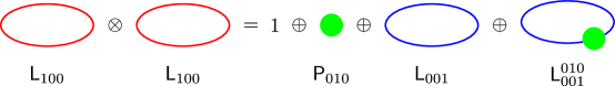
Figure 1: A typical example of fusion rules in $BF$ theory with $AAB$ twisted term. Fusing two loops $\mathsf{L}_{100}$ has four possible fusion channels: the vacuum, the particle $\mathsf{P}_{010}$, the pure loop $\mathsf{L}_{001}$, and the decorated loop $\mathsf{L}_{001}^{010}$.

In $3$D topological order, topological excitations are point-like particles, i.e., anyons. However, in higher-dimensional topological orders, spatially extended topological excitations may occur and we can consider their shrinking rules. For instance, in $4$D, there exist loop excitations and they can be shrunk to point-like particles. Keep lifting dimension to $5$D, spatially extended topological excitations include both loops and membranes. Some membranes can be shrunk to loops first and then shrunk to particles, such shrinking processes are called hierarchical shrinking rules. In path integral representation, we define a shrinking operator $\mathcal{S}$, then shrinking an excitation $\mathsf{a}$ is

$$\langle\mathcal{S}\left(\mathsf{a}\right)\rangle= \langle\underset{X_{1}\rightarrow X_{2}}{\lim}\mathsf{a}\rangle=\underset{X_{1}\rightarrow X_{2}}{\lim}\frac{1}{\mathcal{Z}}\int{\mathcal{D}\left[ABC\right]\exp\left(iS\right)\mathcal{O}_{\mathsf{a}}}=\sum_{\mathsf{b}}\frac{1}{\mathcal{Z}}\int{\mathcal{D}\left[ABC\right]\exp\left(iS\right)\mathrm{S}_{\mathsf{b}}^{\mathsf{a}}\mathcal{O}_{\mathsf{b}}}$$

$$= \langle\oplus_{\mathsf{b}}{\mathrm{S}}_{\mathsf{b}}^{\mathsf{a}}\mathsf{b}\rangle\,,$$ (11)

where $\mathcal{Z}$ and $S$ are partition function and action respectively. $X_{1}$ and $X_{2}$ are respectively spacetime trajectories (manifold) of excitation $\mathsf{a}$ (Wilson operator $\mathcal{O}_{\mathsf{a}}$) before and after shrinking, which respects $X_{2}\subset X_{1}$. We can simply rewrite eq. (11) as

$$\mathcal{S}\left(\mathsf{a}\right)=\oplus_{\mathsf{b}}{\mathrm{S}}_{\mathsf{b}}^{\mathsf{a}}\mathsf{b}\,.$$ (12)

${\mathrm{S}}_{\mathsf{b}}^{\mathsf{a}}\in\mathbb{Z}$ is the shrinking coefficient there are ${\mathrm{S}}_{\mathsf{b}}^{\mathsf{a}}\in\mathbb{Z}$ shrinking channels to $\mathsf{b}$. Summation $\oplus_{\mathsf{b}}$ exhausts all topological excitations in the system. If ${\mathrm{S}}_{\mathsf{b}}^{\mathsf{a}}=0$, then shrinking $\mathsf{a}$ to $\mathsf{b}$ is prohibited. A shrinking process is called Abelian if it has a single shrinking channel, otherwise, it is deemed non-Abelian. Working in the TQFT paradigm, Refs. Huang et al. (2023); Zhang et al. (2023b) show that (hierarchical) shrinking rules respect fusion rules; that is, in $4$D, we have:

$$\mathcal{S}\left(\mathsf{a}\right)\otimes\mathcal{S}\left(\mathsf{b}\right)=\mathcal{S}\left(\mathsf{a}\otimes\mathsf{b}\right)\,.$$ (13)

Eq. (13) only holds for $4$D because we only need one step to shrink loops to particles, which precludes the existence of non-trivial hierarchical shrinking structures. While in $5$D, topological excitations can be particles, loops, and membranes. For a sphere-like membrane, we can directly shrink it to particles. However, for a torus-like membrane, we may first shrink it to a loop and then continue to shrink the loop to a particle. If we need at least two steps to shrink such a membrane to a particle, we say there exist hierarchical shrinking rules. Ref. Huang et al. (2023) shows that for $5$D topological order described by $BF$ field theory, $BBA$ and $AAAB$ twisted terms can lead to nontrivial hierarchical shrinking rules. For $AAAAA$, $AAAdA$, and $AAC$ twisted terms, we find that they have non-Abelian shrinking rules, but their shrinking rules are not hierarchical, i.e., torus-like membranes are shrunk to nontrivial particles and the trivial loop in the first step. Since the trivial loop is equivalent to the vacuum and thus can be ignored, these torus-like membranes are directly shrunk to particles in the first shrinking process. For $AdAdA$, $AdAB$, and $AAdB$ twisted terms, they only admit Abelian shrinking rules and trivial hierarchical shrinking rules. Generally, in $5$D, hierarchical shrinking rules respect fusion rules, that is,

$$\mathcal{S}^{2}\left(\mathsf{a}\right)\otimes\mathcal{S}^{2}\left(\mathsf{b}\right)=\mathcal{S}^{2}\left(\mathsf{a}\otimes\mathsf{b}\right)\,,$$ (14)

where $\mathcal{S}^{2}=\mathcal{S}\mathcal{S}$ means shrinking twice.

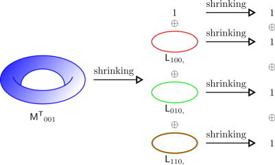
Figure 2: A typical example of hierarchical shrinking rules in $BF$ theory with $BBA$ twisted term. The torus membrane ${\mathsf{M}^{\mathsf{T}}}_{001}$ has four shrinking channels: the vacuum, the loop $\mathsf{L}_{100,}$, the loop $\mathsf{L}_{010,}$, and the loop $\mathsf{L}_{110,}$. Subsequently, these loops are shrunk to vacua.

Following the notations in Ref. Huang et al. (2023), here we calculate an explicit example of shrinking a torus-like membrane ${\mathsf{M}^{\mathsf{T}}}_{001}$ in $BBA$ twisted term:

$$\langle\mathcal{S}\left({\mathsf{M}^{\mathsf{T}}}_{001}\right)\rangle=\langle\underset{\tilde{\omega}\rightarrow\sigma}{\lim}{\mathsf{M}^{\mathsf{T}}}_{001}\rangle=\underset{\tilde{\omega}\rightarrow\sigma}{\lim}\frac{1}{\mathcal{Z}}\int{\mathcal{D}\left[ABC\right]\exp\left(iS\right)}\mathcal{O}_{{\mathsf{M}^{\mathsf{T}}}_{001}}$$

$$= \underset{\tilde{\omega}\rightarrow\sigma}{\lim}\frac{1}{\mathcal{Z}}\int{\mathcal{D}\left[ABC\right]\exp\left(iS\right)}$$

$$\times 4\exp\left[i\int_{\tilde{\omega}}{C^{3}+\frac{1}{2}\frac{2\pi q}{N_{3}}\left(d^{-1}B^{1}B^{2}+d^{-1}B^{2}B^{1}\right)}\right]\delta\left(\int_{\sigma}{B^{1}}\right)\delta\left(\int_{\sigma}{B^{2}}\right)$$

$$= \frac{1}{\mathcal{Z}}\int{\mathcal{D}\left[ABC\right]\exp\left(iS\right)}\times\left[1+\exp\left(i\int_{\sigma}{B^{1}}\right)+\exp\left(i\int_{\sigma}{B^{2}}\right)+\exp\left(i\int_{\sigma}{B^{1}+B^{2}}\right)\right]$$

$$= \frac{1}{\mathcal{Z}}\int{\mathcal{D}\left[ABC\right]\exp\left(iS\right)}\times\left[\mathcal{O}_{1}+\mathcal{O}_{\mathsf{L}_{100,}}+\mathcal{O}_{\mathsf{L}_{010,}}+\mathcal{O}_{\mathsf{L}_{110,}}\right]$$

$$= \langle\mathsf{1}\oplus\mathsf{L}_{100,}\oplus\mathsf{L}_{010,}\oplus\mathsf{L}_{110,}\rangle\,.$$ (15)

Here, $\mathsf{1}$ is the vacuum. $\mathsf{L}_{100,}$ and $\mathsf{L}_{010,}$ are loops carrying a gauge charge of $2$-form field $B^{1}$ and a gauge charge of $2$-form field $B^{2}$ respectively. $\mathsf{L}_{110,}$ is a loop carrying both a gauge charge of $B^{1}$ and a gauge charge of $B^{2}$. ${\mathsf{M}^{\mathsf{T}}}_{001}$ is a torus-like membrane carrying a gauge charge of $3$-form field $C^{3}$. This result means that shrinking the membrane ${\mathsf{M}^{\mathsf{T}}}_{001}$ has four shrinking channels: the vacuum, the loop $\mathsf{L}_{100,}$, the loop $\mathsf{L}_{010,}$, and the loop $\mathsf{L}_{110,}$. These loops can be further shrunk to particles, i.e., the membrane ${\mathsf{M}^{\mathsf{T}}}_{001}$ have hierarchical shrinking rules:

$$\langle\mathcal{S}^{2}\left({\mathsf{M}^{\mathsf{T}}}_{001}\right)\rangle=\langle\mathcal{S}\left(1\oplus\mathsf{L}_{100,}\oplus\mathsf{L}_{010,}\oplus\mathsf{L}_{110,}\right)\rangle=\langle\underset{\sigma\rightarrow\gamma}{\lim}\left(1\oplus\mathsf{L}_{100,}\oplus\mathsf{L}_{010,}\oplus\mathsf{L}_{110,}\right)\rangle$$

$$= \underset{\sigma\rightarrow\gamma}{\lim}\frac{1}{\mathcal{Z}}\int{\mathcal{D}\left[ABC\right]\exp\left(iS\right)}\left[1+\exp\left(i\int_{\sigma}{B^{1}}\right)+\exp\left(i\int_{\sigma}{B^{2}}\right)+\exp\left(i\int_{\sigma}{B^{1}+B^{2}}\right)\right]$$

$$= \frac{1}{\mathcal{Z}}\int{\mathcal{D}\left[ABC\right]\exp\left(iS\right)\times\left[1+\exp\left(i0\right)+\exp\left(i0\right)+\exp\left(i0\right)\right]}$$

$$= \frac{1}{\mathcal{Z}}\int{\mathcal{D}\left[ABC\right]\exp\left(iS\right)\times 4\cdot 1}=\langle 4\cdot\mathsf{1}\rangle\,.$$ (16)

This result indicates that, by performing shrinking twice, ${\mathsf{M}^{\mathsf{T}}}_{001}$ can be shrunk to the vacuum ultimately, as shown in figure 2.

III Fusion and shrinking rules as mappings

In this section, we categorize excitations into different sets and study fusion and shrinking processes as mappings between these sets. Excitations from different sets need to be treated differently in our diagrammatic representations because they play distinct roles in (hierarchical) shrinking processes. Assuming there are only finite topological excitations in a $n$-dimensional topological order, we can list all possible excitations in a set $\Phi_{0}^{n}$, where the superscript $n$ denotes the spacetime dimension. In the following discussion, we interpret shrinking as a mapping from the set $\Phi_{0}^{n}$ to one of its subset, denoted as $\Phi_{1}^{n}$. If hierarchical shrinking rules are nontrivial, we can generally map the subset $\Phi_{i}^{n}$ to a smaller subset $\Phi_{i+1}^{n}$, where $i=0,1,\cdots,n-4$. Additionally, there may exist other subsets with closed fusion rules that cannot be obtained by shrinking, we denote them as $\Phi_{i}^{n}$, where $i\geqslant n-2$.

III.1 4D topological orders

In a $4$D topological order, we generally list all excitations in the set $\Phi_{0}^{4}$:

$$\Phi_{0}^{4}=\left\{\mathsf{1},\mathsf{P}_{1},\mathsf{P}_{2},\cdots\mathsf{P}_{n},\mathsf{L}_{1},\mathsf{L}_{2},\cdots,\mathsf{L}_{m}\right\}\,,$$ (17)

where $\mathsf{1}$ is the vacuum (trivial particle $\mathsf{P}_{0}$ and trivial loop $\mathsf{L}_{0}$ are equivalent to vacuum, i.e., $\mathsf{1}=\mathsf{P}_{0}=\mathsf{L}_{0}$), $\mathsf{P}_{i}$ and $\mathsf{L}_{i}$ denote particles and loops respectively. The possible outcomes of fusing two excitations still form the set $\Phi_{0}^{4}$, thus we can view fusion as a mapping:

$$\otimes:\quad\Phi_{0}^{4}\times\Phi_{0}^{4}\rightarrow\Phi_{0}^{4}\,,$$ (18)

where $\otimes$ means fusion and $\Phi_{0}^{4}\times\Phi_{0}^{4}=\left\{\left(\mathsf{E}_{i},\mathsf{E}_{j}\right)\mid\mathsf{E}_{i}\in\Phi_{0}^{4},\mathsf{E}_{j}\in\Phi_{0}^{4}\right\}$.

The shrinking operator can shrink loops into particles, but it will not alter particles (which means the shrinking operator acts on a particle will give the particle itself). Thus, shrinking can be considered as a mapping from the original set $\Phi_{0}^{4}$ to a subset $\Phi_{1}^{4}$:

$$\mathcal{S}:\quad\Phi_{0}^{4}\rightarrow\Phi_{1}^{4}\,.$$ (19)

$$\Phi_{1}^{4}=\left\{\mathsf{P}_{0},\mathsf{P}_{1},\mathsf{P}_{2},\cdots\mathsf{P}_{n}\right\}\,.$$ (20)

Since particles cannot be further shrunk, $\mathcal{S}:\,\Phi_{1}^{4}\rightarrow\Phi_{1}^{4}$ is trivial. Ref. Zhang et al. (2023b) shows that such subset $\Phi_{1}^{4}$ also have a closed fusion rules, i.e.,

$$\mathsf{P}_{i}\otimes\mathsf{P}_{j}=\oplus_{k}N_{\mathsf{P}_{k}}^{\mathsf{P}_{i}\mathsf{P}_{j}}\mathsf{P}_{k},\qquad i,j,k\in\left\{0,1,\cdots,n\right\}\,.$$ (21)

Thus we can extend eq. (18) to $\otimes:\,\,\Phi_{i}^{4}\times\Phi_{i}^{4}\rightarrow\Phi_{i}^{4}$, where $i=0,1$. Now start from $\Phi_{0}^{4}$, we can consider $\mathcal{S}\left(\cdot\right)\otimes\mathcal{S}\left(\cdot\right)$ and $\mathcal{S}\left(\cdot\otimes\cdot\right)$ as:

$$\mathcal{S}\left(\cdot\right)\otimes\mathcal{S}\left(\cdot\right): \quad\Phi_{0}^{4}\times\Phi_{0}^{4}\rightarrow\Phi_{1}^{4}\times\Phi_{1}^{4}\rightarrow\Phi_{1}^{4}\,,$$ (22)

$$\mathcal{S}\left(\cdot\otimes\cdot\right): \quad\Phi_{0}^{4}\times\Phi_{0}^{4}\rightarrow\Phi_{0}^{4}\rightarrow\Phi_{1}^{4}\,.$$ (23)

Recall eq. (13) in $4$D, shrinking rules respect fusion rules, we conclude that $\mathcal{S}\left(\cdot\right)\otimes\mathcal{S}\left(\cdot\right)$ and $\mathcal{S}\left(\cdot\otimes\cdot\right)$ only differ by intermediate states and they give the same outputs.

III.2 $5$D topological orders

We can generalize the above description to $5$D, where excitations now include particles, loops, and membranes. We can generally list the set $\Phi_{0}^{5}$ as:

$$\Phi_{0}^{5}=\left\{1,\mathsf{P}_{1},\mathsf{P}_{2},\cdots\mathsf{P}_{n},\mathsf{L}_{1},\mathsf{L}_{2},\cdots,\mathsf{L}_{m},\mathsf{M}_{1},\mathsf{M}_{1},\cdots,\mathsf{M}_{k}\right\}\,,$$ (24)

where $\mathsf{1}$ is the vacuum (trivial particle $\mathsf{P}_{0}$, trivial loop $\mathsf{L}_{0}$, and trivial membrane $\mathsf{M}_{0}$ are equivalent to vacuum), $\mathsf{P}_{i}$, $\mathsf{L}_{i}$, and $\mathsf{M}_{i}$ denote particles, loops, and membranes respectively. If we consider nontrivial hierarchical shrinking rules, loops and membranes are shrunk to particles and loops respectively in the first shrinking process, which can be considered as a mapping from the original set $\Phi_{0}^{5}$ to a subset $\Phi_{1}^{5}$:

$$\Phi_{1}^{5}=\left\{1,\mathsf{P}_{1},\mathsf{P}_{2},\cdots\mathsf{P}_{n},\mathsf{L}_{1},\mathsf{L}_{2},\cdots,\mathsf{L}_{p}\right\}\,,$$ (25)

where $p\leqslant m$ because some loops may not appear as shrinking outputs. In fact, Ref. Huang et al. (2023) shows that we have $p\textless m$ for $BBA$ and $AAAB$ twisted terms. (If a system does not have nontrivial hierarchical shrinking rules, then we have $p=0$ and the subset $\Phi_{1}^{5}$ and the subset $\Phi_{2}^{5}$ contain the same excitations). Continue to shrink the excitations in subset $\Phi_{1}^{5}$, we get a smaller subset:

$$\Phi_{2}^{5}=\left\{1,\mathsf{P}_{1},\mathsf{P}_{2},\cdots\mathsf{P}_{n}\right\}\,.$$ (26)

Given the result in Ref. Huang et al. (2023), we can verify that sets $\Phi_{0}^{5}$, $\Phi_{1}^{5}$, and $\Phi_{2}^{5}$ all have closed fusion rules. Also, the subset $\Phi_{3}^{5}$

$$\Phi_{3}^{5}=\left\{1,\mathsf{P}_{1},\mathsf{P}_{2},\cdots\mathsf{P}_{n},\mathsf{L}_{1},\mathsf{L}_{2},\cdots,\mathsf{L}_{m}\right\}\,,$$ (27)

has closed fusion rules and can be mapped to the subset $\Phi_{2}^{5}$ by a shrinking process (however, one cannot map $\Phi_{i}^{5}$ to $\Phi_{3}^{5}$ by a shrinking process). Thus we can consider shrinking and fusion as mappings:

$$\otimes:\,\,\,\,\Phi_{i}^{5}\times\Phi_{i}^{5}\rightarrow\Phi_{i}^{5}\,,\,\,i=0,1,2,3\quad\quad\mathcal{S}:\,\,\,\,\begin{cases}\Phi_{j}^{5}\rightarrow\Phi_{j+1}^{5}\,,j=0,1\\ \Phi_{2}^{5}\rightarrow\Phi_{2}^{5}\,\,\text{(trivial)}\\ \Phi_{3}^{5}\rightarrow\Phi_{2}^{5}\\ \end{cases}$$ (28)

If we consider fusion and shrinking simultaneously, we will find that the original set $\Phi_{0}^{5}$ only admits

$$\mathcal{S}^{2}\left(\mathsf{a}\right)\otimes\mathcal{S}^{2}\left(\mathsf{b}\right)=\mathcal{S}^{2}\left(\mathsf{a}\otimes\mathsf{b}\right)\quad\mathsf{a},\,\mathsf{b}\in\Phi_{0}^{5}\,.$$ (29)

While the subset $\Phi_{1}^{5}$, $\Phi_{2}^{5}$ and $\Phi_{3}^{5}$ admit

$$\mathcal{S}\left(\mathsf{c}\right)\otimes\mathcal{S}\left(\mathsf{d}\right)=\mathcal{S}\left(\mathsf{c}\otimes\mathsf{d}\right)\quad\mathsf{c},\,\mathsf{d}\in\Phi_{1,2,3}^{5}\,.$$ (30)

Eq. (30) is not the most general relation in $5$D because $\mathsf{c}$ and $\mathsf{d}$ can only be particles and loops. Since the subset $\Phi_{1}^{5}$ and $\Phi_{2}^{5}$ can be obtained by acting a shrinking process on $\Phi_{0}^{5}$, i.e., we can always find $\mathsf{a}\in\Phi_{0}^{5}$ and $\mathsf{b}\in\Phi_{0}^{5}$ such that $\mathcal{S}\left(\mathsf{a}\right)$ and $\mathcal{S}\left(\mathsf{b}\right)$ have shrinking channels to $\mathsf{c}\in\Phi_{1,2}^{5}$ and $\mathsf{d}\in\Phi_{1,2}^{5}$ respectively, we have

$$\mathcal{S}^{2}\left(\mathsf{a}\right)\otimes\mathcal{S}^{2}\left(\mathsf{b}\right)=\mathcal{S}\left(\mathcal{S}\left(\mathsf{a}\right)\otimes\mathcal{S}\left(\mathsf{b}\right)\right)$$ (31)

holds for the original set $\Phi_{0}^{5}$. Now, start from $\Phi_{0}^{5}$ in $5$D, we can consider $\mathcal{S}^{2}\left(\cdot\right)\otimes\mathcal{S}^{2}\left(\cdot\right)$, $\mathcal{S}^{2}\left(\cdot\otimes\cdot\right)$ and $\mathcal{S}\left(\mathcal{S}\left(\cdot\right)\otimes\mathcal{S}\left(\cdot\right)\right)$ as :

$$\mathcal{S}^{2}\left(\cdot\right)\otimes\mathcal{S}^{2}\left(\cdot\right): \quad\Phi_{0}^{5}\times\Phi_{0}^{5}\rightarrow\Phi_{1}^{5}\times\Phi_{1}^{5}\rightarrow\Phi_{2}^{5}\times\Phi_{2}^{5}\rightarrow\Phi_{2}^{5}\,,$$ (32)

$$\mathcal{S}^{2}\left(\cdot\otimes\cdot\right): \quad\Phi_{0}^{5}\times\Phi_{0}^{5}\rightarrow\Phi_{0}^{5}\rightarrow\Phi_{1}^{5}\rightarrow\Phi_{2}^{5}\,,$$ (33)

$$\mathcal{S}\left(\mathcal{S}\left(\cdot\right)\otimes\mathcal{S}\left(\cdot\right)\right): \quad\Phi_{0}^{5}\times\Phi_{0}^{5}\rightarrow\Phi_{1}^{5}\times\Phi_{1}^{5}\rightarrow\Phi_{1}^{5}\rightarrow\Phi_{2}^{5}\,.$$ (34)

The three mappings above only differ by intermediate states and they should give the same outputs. If we start from the subset $\Phi_{3}^{5}$, then we have:

$$\mathcal{S}\left(\cdot\right)\otimes\mathcal{S}\left(\cdot\right): \quad\Phi_{3}^{5}\times\Phi_{3}^{5}\rightarrow\Phi_{2}^{5}\times\Phi_{2}^{5}\rightarrow\Phi_{2}^{5}\,,$$ (35)

$$\mathcal{S}\left(\cdot\otimes\cdot\right): \quad\Phi_{3}^{5}\times\Phi_{3}^{5}\rightarrow\Phi_{3}^{5}\rightarrow\Phi_{2}^{5}\,.$$ (36)

The two mappings above only differ by intermediate states. This is similar to the case in $4$D.

Based on these results, we will construct diagrammatic representations of higher-dimensional topological orders in section IV and section V.

IV Construction of diagrammatic representations of $4$D topological orders

In this section, inspired by several results from TQFT, we construct diagrammatic representations of $4$D topological orders that can consistently describe fusion and shrinking rules. From such theory, we obtain a shrinking-fusion hexagon equation for anomalous-free topological orders in $4$D. We will generalize our construction to $5$D in section V.

IV.1 Fusion diagrams: fusion space, $F$-symbols, and pentagon relation

First, we consider constructing fusion diagrams in $4$D. Suppose the fusion process $\mathsf{a}\otimes\mathsf{b}$ has fusion channels to $\mathsf{c}$, we can represent these fusion channels diagrammatically in figure 3. The solid lines can be understood as the spacetime trajectories of excitations. As mentioned in section III.1, we can either fuse two excitations in the set $\Phi_{0}^{4}$ or two excitations in the subset $\Phi_{1}^{4}$, thus we use double-line and single-line to represent excitations from the set $\Phi_{0}^{4}$ and $\Phi_{1}^{4}$ respectively. $\mu=\left\{1,2,\cdots,N_{\mathsf{c}}^{\mathsf{a}\mathsf{b}}\right\}$ labels different fusion channels to $\mathsf{c}$. Notice that if $N_{\mathsf{c}}^{\mathsf{a}\mathsf{b}}=0$, we say diagrams in figure 3 cannot happen. The left diagrams in figure 3 can be defined as a vector $\ket{\mathsf{a},\mathsf{b};\mathsf{c},\mu}_{0}$, different $\mu$ represent orthogonal vectors. This set of vectors $\left\{\ket{\mathsf{a},\mathsf{b};\mathsf{c},\mu}_{0},\mu=1,2,\cdots,N_{\mathsf{c}}^{\mathsf{a}\mathsf{b}}\right\}$ spans a fusion space ${V_{0}}_{\mathsf{c}}^{\mathsf{ab}}$ with $\text{dim}({V_{0}}_{\mathsf{c}}^{\mathsf{ab}})=N_{\mathsf{c}}^{\mathsf{a}\mathsf{b}}$. Similarly, we can define the right diagram in figure 3 as a vector $\ket{\mathsf{a},\mathsf{b};\mathsf{c},\mu}_{1}$ and the corresponding fusion space is ${V_{1}}_{\mathsf{c}}^{\mathsf{ab}}$. Since these two diagrams only differ by single-lines and double lines, we only draw the fusion diagrams for the set $\Phi_{0}^{4}$ in the following discussion and omit the index "$0$" of vectors and spaces. One can easily obtain the diagrams for the set $\Phi_{1}^{4}$ by simply replacing double-lines with single-lines.

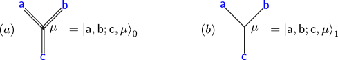
Figure 3: Fusion diagrams. $\mathsf{a}$, $\mathsf{b}$ and $\mathsf{c}$ denote excitations and we use blue to highlight them. $\mu=\left\{1,2,\cdots,N_{\mathsf{c}}^{\mathsf{a}\mathsf{b}}\right\}$ labels different fusion channels with the same outcome $\mathsf{c}$. (a) Double-lines mean that $\mathsf{a},\mathsf{b},\mathsf{c}\in\Phi_{0}^{4}$ and this diagram represents fusion for set $\Phi_{0}^{4}$. (b) Single-lines mean that $\mathsf{a},\mathsf{b},\mathsf{c}\in\Phi_{1}^{4}$ and this diagram represents fusion for set $\Phi_{1}^{4}$.

Now we further consider diagrams that involve more excitations. Suppose fusion process $\left(\mathsf{a}\otimes\mathsf{b}\right)\otimes\mathsf{c}$ has fusion channels to $\mathsf{d}$, diagrammatically we have figure 4. Such a diagram can be constructed by stacking two fusion diagrams shown in figure 3. The diagram in figure 4 can also be defined as a vector $\ket{\left(\mathsf{a},\mathsf{b}\right);\mathsf{e},\mu}\otimes\ket{\mathsf{e},\mathsf{c};\mathsf{d},\nu}$, where $\otimes$ means tensor product. The corresponding space is denoted as $V_{\mathsf{d}}^{\mathsf{a}\mathsf{b}\mathsf{c}}$, whose dimension is $\text{dim}(V_{\mathsf{d}}^{\mathsf{a}\mathsf{b}\mathsf{c}})=\sum_{\mathsf{e}}{N_{\mathsf{e}}^{\mathsf{ab}}}N_{\mathsf{d}}^{\mathsf{ec}}$ because $V_{\mathsf{d}}^{\mathsf{a}\mathsf{b}\mathsf{c}}$ is isomorphic to $\oplus_{\mathsf{e}}V_{\mathsf{e}}^{\mathsf{ab}}\otimes V_{\mathsf{d}}^{\mathsf{ec}}$.

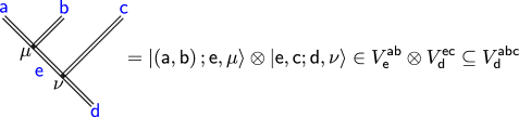
Figure 4: Fusion diagram of three excitations. $\mathsf{a}$, $\mathsf{b}$, and $\mathsf{c}$ are input excitations and they finally fuse to $\mathsf{d}$. We use blue to highlight excitations. The bracket $\left(\mathsf{a}\otimes\mathsf{b}\right)$ means $\mathsf{a}$ and $\mathsf{b}$ fuse together first. $\otimes$ mean tensor product here. The set $\left\{\ket{\left(\mathsf{a},\mathsf{b}\right);\mathsf{e},\mu}\otimes\ket{\mathsf{e},\mathsf{c};\mathsf{d},\nu}\right\}$ spans the whole space $V_{\mathsf{d}}^{\mathsf{abc}}$, different $\mu$, $\nu$ and $\mathsf{e}$ label different orthogonal vectors. The space $V_{\mathsf{d}}^{\mathsf{abc}}$ is isomorphic to $\oplus_{\mathsf{e}}V_{\mathsf{e}}^{\mathsf{ab}}\otimes V_{\mathsf{d}}^{\mathsf{ec}}$, where $\oplus$ means direct sum. The dimension of $V_{\mathsf{d}}^{\mathsf{a}\mathsf{b}\mathsf{c}}$ is given by $\text{dim}(V_{\mathsf{d}}^{\mathsf{a}\mathsf{b}\mathsf{c}})=\sum_{\mathsf{e}}{N_{\mathsf{e}}^{\mathsf{ab}}}N_{\mathsf{d}}^{\mathsf{ec}}$. Here we only draw the diagram for fusion process in the set $\Phi_{0}^{4}$ and simply write $\ket{\left(\mathsf{a},\mathsf{b}\right);\mathsf{e},\mu}_{0}$ and ${V_{0}}_{\mathsf{e}}^{\mathsf{ab}}$ as $\ket{\left(\mathsf{a},\mathsf{b}\right);\mathsf{e},\mu}$ and ${V}_{\mathsf{e}}^{\mathsf{ab}}$ respectively. One can obtain the diagram for subset $\Phi_{1}^{4}$ by simply replacing all double-lines with single-lines.

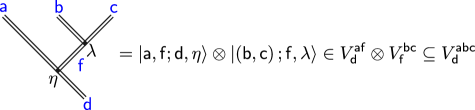
Figure 5: A different diagram of fusing three excitations. The associativity of fusion rules guarantees that this diagram actually describes the same physics as the diagram shown in figure 4. The only difference between them is just a change of basis.

As we mentioned in section III, physically, fusion rules have an important property known as associativity, i.e., $\left(\mathsf{a}\otimes\mathsf{b}\right)\otimes\mathsf{c}=\mathsf{a}\otimes\left(\mathsf{b}\otimes\mathsf{c}\right)$. This means that fusing $\mathsf{b}$ and $\mathsf{c}$ first should gives the same final result as fusing $\mathsf{a}$ and $\mathsf{b}$ first. Thus the diagram shown in figure 5 also represents a set of basis vectors in $V_{\mathsf{d}}^{\mathsf{abc}}$. Actually, figure 4 and figure 5 represent different bases and we can use a unitary matrix, known as $F$-symbol, to change the basis. The definition of $F$-symbol is given by figure 6. We can express the equation in figure 6 as:

$$\ket{\left(\mathsf{a},\mathsf{b}\right);\mathsf{e},\mu}\otimes\ket{\mathsf{e},\mathsf{c};\mathsf{d},\nu}=\sum_{\mathsf{f},\lambda,\eta}{\left[F_{\mathsf{d}}^{\mathsf{abc}}\right]_{\mathsf{e}\mu\nu,\mathsf{f}\lambda\eta}}\ket{\mathsf{a},\mathsf{f};\mathsf{d},\eta}\otimes\ket{\left(\mathsf{b},\mathsf{c}\right);\mathsf{f},\lambda}\,.$$ (37)

The summation over $\mathsf{f}$ exhausts all excitations in the system, $\lambda=\left\{1,2,\cdots,N_{\mathsf{f}}^{\mathsf{bc}}\right\}$ and $\eta=\left\{1,2,\cdots,N_{\mathsf{d}}^{\mathsf{af}}\right\}$. Since $F$-symbol is unitary, we have

$$\sum_{\mathsf{f},\lambda,\eta}{\left[F_{\mathsf{d}}^{\mathsf{abc}}\right]_{\mathsf{e}\mu\nu,\mathsf{f}\lambda\eta}}\left(\left[F_{\mathsf{d}}^{\mathsf{abc}}\right]_{\mathsf{e}^{\prime}\mu^{\prime}\nu^{\prime},\mathsf{f}\lambda\eta}\right)^{\ast}=\delta_{\mathsf{ee}^{\prime}}\delta_{\mu\mu^{\prime}}\delta_{\nu\nu^{\prime}}\,,$$ (38)

and we can draw figure 7. We can also derive a constraint of fusion coefficients by comparing the dimension of $V_{\mathsf{d}}^{\mathsf{a}\mathsf{b}\mathsf{c}}$ calculated from figure 4 and figure 5, where the total space $V_{\mathsf{d}}^{\mathsf{abc}}$ is constructed by $\oplus_{\mathsf{e}}V_{\mathsf{e}}^{\mathsf{ab}}\otimes V_{\mathsf{d}}^{\mathsf{ec}}$ and $\oplus_{\mathsf{f}}V_{\mathsf{d}}^{\mathsf{af}}\otimes V_{\mathsf{f}}^{\mathsf{bc}}$ respectively. Thus

$$\text{dim}(V_{\mathsf{d}}^{\mathsf{a}\mathsf{b}\mathsf{c}})=\sum_{\mathsf{e}}{N_{\mathsf{e}}^{\mathsf{ab}}}N_{\mathsf{d}}^{\mathsf{ec}}=\sum_{\mathsf{f}}{N_{\mathsf{d}}^{\mathsf{af}}}N_{\mathsf{f}}^{\mathsf{bc}}\,.$$ (39)

This formula can also be derived by directly using associativity and eq. (6):

$$\left(\mathsf{a}\otimes\mathsf{b}\right)\otimes\mathsf{c}=\left(\oplus_{\mathsf{e}}N_{\mathsf{e}}^{\mathsf{ab}}\mathsf{e}\right)\otimes\mathsf{c}=\oplus_{\mathsf{ed}}N_{\mathsf{e}}^{\mathsf{ab}}N_{\mathsf{d}}^{\mathsf{ec}}\mathsf{d}\,,$$ (40)

$$\mathsf{a}\otimes\left(\mathsf{b}\otimes\mathsf{c}\right)=\mathsf{a}\otimes\left(\oplus_{\mathsf{f}}N_{\mathsf{f}}^{\mathsf{bc}}\mathsf{f}\right)=\oplus_{\mathsf{fd}}N_{\mathsf{f}}^{\mathsf{bc}}N_{\mathsf{d}}^{\mathsf{af}}\mathsf{d}\,.$$ (41)

Comparing the fusion coefficients, we have:

$$\sum_{\mathsf{e}}{N_{\mathsf{e}}^{\mathsf{ab}}}N_{\mathsf{d}}^{\mathsf{ec}}=\sum_{\mathsf{f}}{N_{\mathsf{d}}^{\mathsf{af}}}N_{\mathsf{f}}^{\mathsf{bc}}\,.$$ (42)

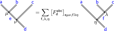
Figure 6: Definition of $F$-symbol. The left and right diagrams describe the same physics in different bases. We use unitary $F$-symbol to change the basis.

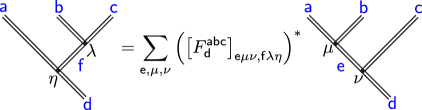
Figure 7: Inverse transformation. This figure comes from the unitarity of $F$-symbols. We use the star to denote complex conjugate.

For other diagrams involving more excitations, we use a similar tensor product to write down the corresponding vectors. Also, $F$-symbols can be applied inside of more complicated diagrams. For example, consider fusing four excitations, we have different ways to transform one diagram into another. As shown in figure 8, we have two paths to transform the far left diagram into the far right diagram, which imposes a very strong constraint on $F$-symbols, known as the pentagon equation:

$$\sum_{\sigma=1}^{N_{\mathsf{e}}^{\mathsf{fh}}}{\left[F_{\mathsf{e}}^{\mathsf{fcd}}\right]_{\mathsf{g}\nu\lambda,\mathsf{h}\gamma\sigma}}\left[F_{\mathsf{e}}^{\mathsf{abh}}\right]_{\mathsf{f}\mu\sigma,\mathsf{i}\rho\delta}=\sum_{\mathsf{j}}{\sum_{\omega=1}^{N_{\mathsf{g}}^{\mathsf{aj}}}{\sum_{\theta=1}^{N_{\mathsf{j}}^{\mathsf{bc}}}{\sum_{\tau=1}^{N_{\mathsf{i}}^{\mathsf{jd}}}{\left[F_{\mathsf{g}}^{\mathsf{abc}}\right]_{\mathsf{f}\mu\nu,\mathsf{j}\theta\omega}\left[F_{\mathsf{e}}^{\mathsf{ajd}}\right]_{\mathsf{g}\omega\lambda,\mathsf{i}\tau\delta}\left[F_{\mathsf{i}}^{\mathsf{bcd}}\right]_{\mathsf{j}\theta\tau,\mathsf{h}\gamma\rho}}}}}\,.$$ (43)

Such pentagon equation also exists in diagrammatic representations of $3$D anyons and it has been proven that no more identities beyond the pentagon equation can be derived by drawing more complicated fusion diagrams. Essentially, the pentagon equation in any dimension comes from the associativity of the fusion rules, we conclude that in any dimension no more identities can be derived from fusion diagrams. If we draw all previous fusion diagrams in a single-line fashion, then our fusion diagrams reduce to $3$D anyonic fusion diagrams. A brief review of $3$D anyon diagrams is shown in appendix A.

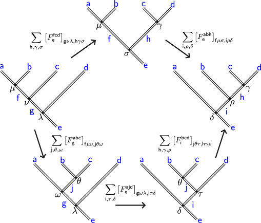
Figure 8: Diagrammatic representation of the pentagon equation (43). We use blue to highlight the excitations. Starting from the far left diagram, we can go to the far right diagram through either the upper path or the lower path. Comparing these two different paths, we can derive the pentagon equation.

IV.2 Shrinking diagrams: shrinking space and $\Delta$-symbol

Suppose for $\mathsf{a}\in\Phi_{0}^{4}$, $\mathcal{S}\left(\mathsf{a}\right)$ has shrinking channels to $\mathsf{b}\in\Phi_{1}^{4}$, then we define the corresponding shrinking diagram in figure 9. We use a triangle to represent the shrinking process. Note that in a specific diagram, a double-line and a single-line may actually represent the same particle, but the double-line and the single-line still have different meanings: the former means that this particle is treated as the input of the shrinking process while the latter means that this particle is the output. Similar to the fusion diagram, the shrinking diagram in figure 9 can be understood as a vector $\ket{\mathsf{a};\mathsf{b},\mu}$. The orthogonal set $\left\{\ket{\mathsf{a};\mathsf{b},\mu},\mu=1,2,\cdots,\mathrm{S}_{\mathsf{b}}^{\mathsf{a}}\right\}$ spans shrinking space $V_{\mathsf{b}}^{\mathsf{a}}$, whose dimension is $\mathrm{dim}\left(V_{\mathsf{b}}^{\mathsf{a}}\right)=\mathrm{S}_{\mathsf{b}}^{\mathsf{a}}$. Here we do not consider $\mathsf{a}\in\Phi_{1}^{4}$ because in section III.1 we have shown that shrinking excitations in the subset $\Phi_{1}^{4}$ is trivial.

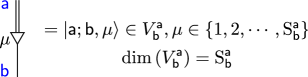
Figure 9: Shrinking diagram. The double-line means that the excitation $\mathsf{a}$ is the input of the shrinking process and thus $\mathsf{a}$ can be a loop or a particle. The single-line means that the excitation $\mathsf{b}$ is the output of the shrinking process and thus $\mathsf{b}$ can only be a particle. We use a triangle to represent the shrinking process. This diagram describes shrinking $\mathsf{a}$ to $\mathsf{b}$ in $\mu$ channel and we define it as a vector. The orthogonal set $\left\{\ket{\mathsf{a};\mathsf{b},\mu},\mu=1,2,\cdots,\mathrm{S}_{\mathsf{b}}^{\mathsf{a}}\right\}$ spans the shrinking space $V_{\mathsf{b}}^{\mathsf{a}}$ with $\mathrm{dim}\left(V_{\mathsf{b}}^{\mathsf{a}}\right)=\mathrm{S}_{\mathsf{b}}^{\mathsf{a}}$.

Now we use tensor product to incorporate fusion and shrinking processes in a diagram. Consider $\mathcal{S}\left(\mathsf{a}\right)\otimes\mathcal{S}\left(\mathsf{b}\right)$ and $\mathcal{S}\left(\mathsf{a}\otimes\mathsf{b}\right)$, their corresponding diagrams are shown as the upper diagram and the lower diagram in figure 10 respectively. Recall eq. (13), shrinking rules respect fusion rules, thus if $\mathcal{S}\left(\mathsf{a}\right)\otimes\mathcal{S}\left(\mathsf{b}\right)$ finally gives $\mathsf{c}$, then $\mathcal{S}\left(\mathsf{a}\otimes\mathsf{b}\right)$ must also give $\mathsf{c}$. Although these two processes have the same final output, they experience different intermediate steps. For the upper diagram in figure 10, $\mathsf{a}$ and $\mathsf{b}$ shrink to $\mathsf{d}$ and $\mathsf{e}$ in $\mu$ and $\nu$ channel respectively first, then $\mathsf{d}$ and $\mathsf{e}$ fuse to $\mathsf{c}$ in $\lambda$ channel. In a non-Abelian case, different legitimate choices of $\mathsf{d}$, $\mathsf{e}$, $\mu$, $\nu$, and $\lambda$ may exist, i.e. they can finally produce $\mathsf{c}$. We define such diagram as $\ket{\mathsf{d},\mathsf{e};\mathsf{c},\lambda}\otimes\ket{\mathsf{b};\mathsf{e},\nu}\otimes\ket{\mathsf{a};\mathsf{d},\mu}$, since $\mathsf{a}$, $\mathsf{b}$ and $\mathsf{c}$ are already fixed, different $\mathsf{d}$, $\mathsf{e}$, $\mu$, $\nu$, and $\lambda$ label different vectors. Exhaust all possible $\mathsf{d}$, $\mathsf{e}$, $\mu$, $\nu$, and $\lambda$, we obtain a set of orthogonal vectors and they span a space denoted as $V_{\mathsf{c}}^{\mathcal{S}\left(\mathsf{a}\right)\otimes\mathcal{S}\left(\mathsf{b}\right)}$, which is isomorphic to $\oplus_{\mathsf{de}}V_{\mathsf{c}}^{\mathsf{de}}\otimes V_{\mathsf{e}}^{\mathsf{b}}\otimes V_{\mathsf{d}}^{\mathsf{a}}$ due to our tensor product construction. For the lower diagram in figure 10, $\mathsf{a}$ and $\mathsf{b}$ fuse to $\mathsf{f}$ in $\delta$ channel first and then $\mathsf{f}$ shrinks to $\mathsf{c}$ in $\gamma$ channel. We define such diagram as $\ket{\mathsf{f};\mathsf{c},\gamma}\otimes\ket{\mathsf{a},\mathsf{b};\mathsf{f},\delta}$, similarly, $\mathsf{a}$, $\mathsf{b}$, and $\mathsf{c}$ are fixed and different legitimate choices of $\mathsf{f}$, $\delta$, and $\gamma$ may exist, thus they label different orthogonal vectors. Exhaust all possible $\mathsf{f}$, $\delta$, and $\gamma$ we obtain a set of vectors and they span a space $V_{\mathsf{c}}^{\mathcal{S}\left(\mathsf{a}\otimes\mathsf{b}\right)}$, which is isomorphic to $\oplus_{\mathsf{f}}V_{\mathsf{c}}^{\mathsf{f}}\otimes V_{\mathsf{f}}^{\mathsf{ab}}$. The conclusion that shrinking rules respect fusion rules also implies that the space $V_{\mathsf{c}}^{\mathcal{S}\left(\mathsf{a}\right)\otimes\mathcal{S}\left(\mathsf{b}\right)}$ is isomorphic to $V_{\mathsf{c}}^{\mathcal{S}\left(\mathsf{a}\otimes\mathsf{b}\right)}$, which leads to:

$$\mathrm{dim}\left(V_{\mathsf{c}}^{\mathcal{S}\left(\mathsf{a}\right)\otimes\mathcal{S}\left(\mathsf{b}\right)}\right)=\mathrm{dim}\left(V_{\mathsf{c}}^{\mathcal{S}\left(\mathsf{a}\otimes\mathsf{b}\right)}\right)=\sum_{\mathsf{de}}{N_{\mathsf{c}}^{\mathsf{de}}\mathrm{S}_{\mathsf{e}}^{\mathsf{b}}\mathrm{S}_{\mathsf{d}}^{\mathsf{a}}}=\sum_{\mathsf{f}}{\mathrm{S}_{\mathsf{c}}^{\mathsf{f}}N_{\mathsf{f}}^{\mathsf{ab}}}\,.$$ (44)

Eq. (44) can also be found in Ref. Zhang et al. (2023b), where all fusion and shrinking rules in the $BF$ theory with $AAB$ twisted term are obtained. Also, eq. (44) is numerically verified. This constraint on fusion coefficients and shrinking coefficients can be considered as a consistency condition for fusion rules and shrinking rules in anomaly-free $4$D topological orders.

The two sets of vectors shown in figure 10 are two different bases of the total space $V_{\mathsf{c}}^{\mathcal{S}\left(\mathsf{a}\right)\otimes\mathcal{S}\left(\mathsf{b}\right)}$ (or equivalently, we can write $V_{\mathsf{c}}^{\mathcal{S}\left(\mathsf{a}\otimes\mathsf{b}\right)}$ here) and thus we expect that they can transform to each other by a unitary matrix, called $\Delta$-symbol. The definition of $\Delta$-symbol is shown in figure 11. We can explicitly write down the transformations in figure 11 as:

$$\ket{\mathsf{d},\mathsf{e};\mathsf{c},\lambda}\otimes\ket{\mathsf{b};\mathsf{e},\nu}\otimes\ket{\mathsf{a};\mathsf{d},\mu}=\sum_{\mathsf{f},\delta,\gamma}{\left[\Delta_{\mathsf{c}}^{\mathsf{ab}}\right]_{\mathsf{de}\mu\nu\lambda,\mathsf{f}\delta\gamma}\ket{\mathsf{f};\mathsf{c},\gamma}\otimes\ket{\mathsf{a},\mathsf{b};\mathsf{f},\delta}}\,,$$ (45)

$$\ket{\mathsf{f};\mathsf{c},\gamma}\otimes\ket{\mathsf{a},\mathsf{b};\mathsf{f},\delta}=\sum_{\mathsf{d},\mathsf{e},\mu,\nu,\lambda}{\left(\left[\Delta_{\mathsf{c}}^{\mathsf{ab}}\right]_{\mathsf{de}\mu\nu\lambda,\mathsf{f}\delta\gamma}\right)^{\ast}\ket{\mathsf{d},\mathsf{e};\mathsf{c},\lambda}\otimes\ket{\mathsf{b};\mathsf{e},\nu}\otimes\ket{\mathsf{a};\mathsf{d},\mu}}\,.$$ (46)

Unitarity of $\Delta$-symbols demands:

$$\sum_{\mathsf{f},\delta,\gamma}{\left[\Delta_{\mathsf{c}}^{\mathsf{ab}}\right]_{\mathsf{de}\mu\nu\lambda,\mathsf{f}\delta\gamma}\left(\left[\Delta_{\mathsf{c}}^{\mathsf{ab}}\right]_{\mathsf{d}^{\prime}\mathsf{e}^{\prime}\mu^{\prime}\nu^{\prime}\lambda^{\prime},\mathsf{f}\delta\gamma}\right)}^{\ast}=\delta_{\mathsf{dd}^{\prime}}\delta_{\mathsf{ee}^{\prime}}\delta_{\mu\mu^{\prime}}\delta_{\nu\nu^{\prime}}\delta_{\lambda\lambda^{\prime}}\,,$$ (47)

$$\sum_{\mathsf{d},\mathsf{e},\mu,\nu,\lambda}{\left[\Delta_{\mathsf{c}}^{\mathsf{ab}}\right]_{\mathsf{de}\mu\nu\lambda,\mathsf{f}\delta\gamma}\left(\left[\Delta_{\mathsf{c}}^{\mathsf{ab}}\right]_{\mathsf{de}\mu\nu\lambda,\mathsf{f}^{\prime}\delta^{\prime}\gamma^{\prime}}\right)^{\ast}}=\delta_{\mathsf{ff}^{\prime}}\delta_{\delta\delta^{\prime}}\delta_{\gamma\gamma^{\prime}}\,.$$ (48)

The element of $\Delta$-symbol $\left[\Delta_{\mathsf{c}}^{\mathsf{ab}}\right]_{\mathsf{de}\mu\nu\lambda,\mathsf{f}\delta\gamma}$ is zero if the corresponding diagram is not allowed. Although we only use diagrams that involve shrinking and fusing two excitations to define $\Delta$-symbol, we are allowed to act a $\Delta$-symbol on a part of a larger diagram, such as the diagram shown in figure 12.

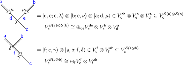
Figure 10: Incorporating fusion and shrinking processes. The upper diagram describes $\mathcal{S}\left(\mathsf{a}\right)\otimes\mathcal{S}\left(\mathsf{b}\right)$ while the lower diagram describes $\mathcal{S}\left(\mathsf{a}\otimes\mathsf{b}\right)$. These diagrams can be constructed by tensoring smaller diagrams. $\otimes$ means tensor product, $\oplus$ means direct sum and $\cong$ means isomorphic to. We can verify that $\mathrm{dim}\left(V_{\mathsf{c}}^{\mathcal{S}\left(\mathsf{a}\right)\otimes\mathcal{S}\left(\mathsf{b}\right)}\right)=\sum_{\mathsf{de}}{N_{\mathsf{c}}^{\mathsf{de}}\mathrm{S}_{\mathsf{e}}^{\mathsf{b}}\mathrm{S}_{\mathsf{d}}^{\mathsf{a}}}$ and $\mathrm{dim}\left(V_{\mathsf{c}}^{\mathcal{S}\left(\mathsf{a}\otimes\mathsf{b}\right)}\right)=\sum_{\mathsf{f}}{\mathrm{S}_{\mathsf{c}}^{\mathsf{f}}N_{\mathsf{f}}^{\mathsf{ab}}}$.

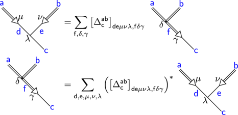
Figure 11: Definition of $\Delta$-symbol. The left diagram and the right diagram describe the same physics in different bases. Similar to the $F$-symbol, the $\Delta$-symbol is also unitary and we can use it to change bases.

IV.3 Shrinking-fusion hexagon equation

In $4$D, fusion rules in both set $\Phi_{0}^{4}$ and subset $\Phi_{1}^{4}$ are still closed and satisfy the associativity: $\left(\mathsf{a}\otimes\mathsf{b}\right)\otimes\mathsf{c}=\mathsf{a}\otimes\left(\mathsf{b}\otimes\mathsf{c}\right)$, which means we can use the $F$-symbols to change the bases when we consider diagrams involve fusing three excitations, regardless which set do these excitations come from. We conclude that by applying the $F$-symbols and $\Delta$-symbols inside of diagrams involving three excitations, we can obtain another consistency relation called the shrinking-fusion hexagon equation besides the pentagon equation. As shown in figure 12, both the upper and lower paths can transform the far left diagram (i.e., $\left(\mathcal{S}\left(\mathsf{a}\right)\otimes\mathcal{S}\left(\mathsf{b}\right)\right)\otimes\mathcal{S}\left(\mathsf{c}\right)$) to the far right diagram (i.e., $\mathcal{S}\left(\mathsf{a}\otimes\left(\mathsf{b}\otimes\mathsf{c}\right)\right)$), these two paths correspond to:

$$\mathrm{far}\,\,\mathrm{left}=\sum_{\mathsf{i},\alpha,\beta,\mathsf{j},\tau,\xi,\mathsf{k},\theta,\epsilon}{\left[F_{\mathsf{d}}^{\mathsf{efg}}\right]_{\mathsf{h}\delta\gamma,\mathsf{i}\alpha\beta}\left[\Delta_{\mathsf{i}}^{\mathsf{bc}}\right]_{\mathsf{fg}\nu\lambda\alpha,\mathsf{j}\tau\xi}\left[\Delta_{\mathsf{d}}^{\mathsf{aj}}\right]_{\mathsf{ei}\mu\xi\beta,\mathsf{k}\theta\epsilon}\mathrm{far}\,\,\mathrm{right}}\,,$$ (49)

$$\mathrm{far}\,\,\mathrm{left}=\sum_{\mathsf{t},\sigma,\rho,\mathsf{k},\omega,\epsilon,\mathsf{j},\tau,\theta}{\left[\Delta_{\mathsf{h}}^{\mathsf{ab}}\right]_{\mathsf{ef}\mu\nu\delta,\mathsf{t}\sigma\rho}\left[\Delta_{\mathsf{d}}^{\mathsf{tc}}\right]_{\mathsf{hg}\rho\lambda\gamma,\mathsf{k}\omega\epsilon}\left[F_{\mathsf{k}}^{\mathsf{abc}}\right]_{\mathsf{t}\sigma\omega,\mathsf{j}\tau\theta}\mathrm{far}\,\,\mathrm{right}}\,,$$ (50)

respectively. Notice that the far right diagram is labeled by $\mathsf{j},\mathsf{k},\tau,\theta$, and $\epsilon$, comparing the coefficients of the far right diagrams in eq. (49) and eq. (50), we obtain a constraint on both the $F$-symbols and $\Delta$-symbols:

$$\sum_{\mathsf{i}}{\sum_{\alpha=1}^{N_{\mathsf{i}}^{\mathsf{fg}}}{\sum_{\beta=1}^{N_{\mathsf{d}}^{\mathsf{ei}}}{\sum_{\xi=1}^{\mathrm{S}_{\mathsf{i}}^{\mathsf{j}}}{\left[F_{\mathsf{d}}^{\mathsf{efg}}\right]_{\mathsf{h}\delta\gamma,\mathsf{i}\alpha\beta}\left[\Delta_{\mathsf{i}}^{\mathsf{bc}}\right]_{\mathsf{fg}\nu\lambda\alpha,\mathsf{j}\tau\xi}\left[\Delta_{\mathsf{d}}^{\mathsf{aj}}\right]_{\mathsf{ei}\mu\xi\beta,\mathsf{k}\theta\epsilon}}}}}$$

$$= \sum_{\mathsf{t}}{\sum_{\sigma=1}^{N_{\mathsf{t}}^{\mathsf{ab}}}{\sum_{\rho=1}^{\mathrm{S}_{\mathsf{h}}^{\mathsf{t}}}{\sum_{\omega=1}^{N_{\mathsf{k}}^{\mathsf{tc}}}{\left[\Delta_{\mathsf{h}}^{\mathsf{ab}}\right]_{\mathsf{ef}\mu\nu\delta,\mathsf{t}\sigma\rho}\left[\Delta_{\mathsf{d}}^{\mathsf{tc}}\right]_{\mathsf{hg}\rho\lambda\gamma,\mathsf{k}\omega\epsilon}}}}}\left[F_{\mathsf{k}}^{\mathsf{abc}}\right]_{\mathsf{t}\sigma\omega,\mathsf{j}\tau\theta}\,.$$ (51)

This shrinking-fusion hexagon equation is a key equation in our $4$D diagrammatic representations, which can be understood as the consistency relation between the $F$-symbols and $\Delta$-symbols. Since being able to use the $\Delta$-symbols to change basis requires the consistency relation between fusion and shrinking coefficients (i.e., eq. (44)) holds, we conclude that the shrinking-fusion hexagon equation actually implies eq. (44). Therefore, the shrinking-fusion hexagon equation is a stronger constraint on consistent fusion and shrinking rules, it describes not only the behavior of fusion and shrinking coefficients but also the transformation of bases. We conjecture that such shrinking-fusion hexagon is universal and all anomaly-free $4$D topological orders should have consistent fusion and shrinking rules and thus satisfy this equation.

We can further consider applying the $F$-symbols and $\Delta$-symbols inside of diagrams involving more excitations, such as starting from the diagram for $\mathcal{S}\left(\mathsf{a}\right)\otimes\mathcal{S}\left(\mathsf{b}\right)\otimes\mathcal{S}\left(\mathsf{c}\right)\otimes\mathcal{S}\left(\mathsf{d}\right)$ and then implement basis transformations. However, we can verify that no more independent equations can be obtained from the diagram involving four excitations. Details can be found in appendix B. We further conjecture that no more independent equations can be obtained from diagrams involving more excitations.

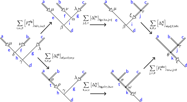
Figure 12: Diagrammatic representations of the shrinking-fusion hexagon equation (51). Two different paths can be constructed to transform the far left diagram to the far right diagram. Comparing these two different paths, we obtain the shrinking-fusion hexagon equation.

V Construction of diagrammatic representations of $5$D topological orders

The idea of constructing the diagrammatic representations of $4$D topological orders can be generalized to $5$D, where nontrivial hierarchical shrinking rules may appear. An anomaly-free $5$D topological order should have consistent fusion and shrinking rules. If there exist nontrivial hierarchical shrinking rules, we further demand that such hierarchical shrinking rules are also consistent with fusion and shrinking rules, which leads to the hierarchical shrinking-fusion hexagon.

V.1 Fusion diagrams

The construction of fusion diagrams in section IV.1 can be easily generalized to $5$D. We can simply replace double-lines by triple-lines in the previous fusion diagrams to represent fusing two excitations in the set $\Phi_{0}^{5}$ (see eq. (24)). Double-lines and single-lines in $5$D represent excitations from the subset $\Phi_{1}^{5}$ and $\Phi_{2}^{5}$ respectively (Actually double-lines can also represent excitations from the subset $\Phi_{3}^{5}$, but since we want to discuss hierarchical shrinking and subset $\Phi_{3}^{5}$ cannot be obtained by shrinking the set $\Phi_{0}^{5}$, we do not consider fusion and shrinking diagrams for the subset $\Phi_{3}^{5}$ in the following context). The definition of the $F$-symbols and pentagon equation in section IV.1 are still valid, figure 6,  7 and 8 can be drawn in triple-, double- and single-line fashions.

V.2 Hierarchical shrinking diagrams and $\Delta^{2}$-symbols

Suppose $\mathsf{a}$ have nontrivial hierarchical shrinking rules and $\mathcal{S}^{2}\left(\mathsf{a}\right)$ gives $\mathsf{c}$ finally, then we define the corresponding hierarchical shrinking diagram in figure 13. Triangle represents the shrinking process, triple-line, double-line, and single-line represent excitations in set $\Phi_{0}^{5}$, $\Phi_{1}^{5}$, and $\Phi_{2}^{5}$ respectively. Similar to the case in $4$D, although these three kinds of lines may represent the same excitation in a specific diagram, they still have different meanings. Different lines indicate different roles (input or output) in the hierarchical shrinking process. Diagram in figure 13 can be understood as a vector $\ket{\mathsf{b};\mathsf{c},\nu}\otimes\ket{\mathsf{a};\mathsf{b},\mu}$. Generally, there are different legitimate $\mathsf{b}$, $\mu$, and $\nu$ that can finally give the desire output $\mathsf{c}$, and thus different $\mathsf{b}$, $\mu$, and $\nu$ thus label different orthogonal vectors. The orthogonal set $\left\{\ket{\mathsf{b};\mathsf{c},\nu}\otimes\ket{\mathsf{a};\mathsf{b},\mu}\right\}$ spans the total shrinking space $V^{\text{total}}$. Such total shrinking space is isomorphic to $\oplus_{\mathsf{b}}V_{\mathsf{c}}^{\mathsf{b}}\otimes V_{\mathsf{b}}^{\mathsf{a}}$, thus we can calculate its dimension as:

$$\mathrm{dim}\left(V^{\mathrm{total}}\right)=\mathrm{dim}\left(\oplus_{\mathsf{b}}V_{\mathsf{c}}^{\mathsf{b}}\otimes V_{\mathsf{b}}^{\mathsf{a}}\right)=\sum_{\mathsf{b}}{\mathrm{S}_{\mathsf{c}}^{\mathsf{b}}\mathrm{S}_{\mathsf{b}}^{\mathsf{a}}}\,.$$ (52)

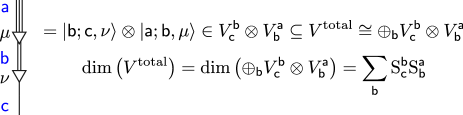
Figure 13: Hierarchical shrinking diagram. Triangle represents the shrinking process, triple-line, double-line, and single-line represent excitations in set $\Phi_{0}^{5}$, $\Phi_{1}^{5}$, and $\Phi_{2}^{5}$ respectively. This diagram describes excitation $\mathsf{a}$ shrinks to $\mathsf{b}$ in $\mu$ channel first, then $\mathsf{b}$ shrinks to $\mathsf{c}$ in $\nu$ channel. The whole diagram can be considered as a vector in the total shrinking space, which is isomorphic to $\oplus_{\mathsf{b}}V_{\mathsf{c}}^{\mathsf{b}}\otimes V_{\mathsf{b}}^{\mathsf{a}}$. Different ways for shrinking $\mathsf{a}$ to $\mathsf{c}$ correspond to different $\mathsf{b}$, $\mu$, and $\nu$, thus correspond to different orthogonal vectors.

Having defined the hierarchical shrinking diagram, we can further consider representing $\mathcal{S}^{2}\left(\mathsf{a}\right)\otimes\mathcal{S}^{2}\left(\mathsf{b}\right)$, $\mathcal{S}^{2}\left(\mathsf{a}\otimes\mathsf{b}\right)$ and $\mathcal{S}\left(\mathcal{S}\left(\mathsf{a}\right)\otimes\mathcal{S}\left(\mathsf{b}\right)\right)$ diagrammatically. As shown in figure 14, we stack shrinking diagrams and fusion diagrams to describe the processes above. These diagrams are still understood as vectors and they can be constructed by tensor product. Since in $5$D, hierarchical shrinking rules respect fusion rules: $\mathcal{S}^{2}\left(\mathsf{a}\right)\otimes\mathcal{S}^{2}\left(\mathsf{b}\right)=\mathcal{S}^{2}\left(\mathsf{a}\otimes\mathsf{b}\right)$, we can expect that diagrams for $\mathcal{S}^{2}\left(\mathsf{a}\right)\otimes\mathcal{S}^{2}\left(\mathsf{b}\right)$, $\mathcal{S}^{2}\left(\mathsf{a}\otimes\mathsf{b}\right)$ describe the same physics. Also, as mentioned in section III.2, for particles and loops, the relation $\mathcal{S}\left(\mathsf{c}\right)\otimes\mathcal{S}\left(\mathsf{d}\right)=\mathcal{S}\left(\mathsf{c}\otimes\mathsf{d}\right)$ still holds. In $5$D, for any excitation $\mathsf{c}\in\Phi_{1,2}^{5}$, we can always find an $\mathsf{a}\in\Phi_{0}^{5}$ such that $\mathcal{S}\left(\mathsf{a}\right)$ has shrinking channels to $\mathsf{c}$, thus we can replace $\mathsf{c}$ and $\mathsf{d}$ with $\mathcal{S}\left(\mathsf{a}\right)$ and $\mathcal{S}\left(\mathsf{b}\right)$ respectively and obtain $\mathcal{S}^{2}\left(\mathsf{a}\right)\otimes\mathcal{S}^{2}\left(\mathsf{b}\right)=\mathcal{S}\left(\mathcal{S}\left(\mathsf{a}\right)\otimes\mathcal{S}\left(\mathsf{b}\right)\right)$. Similarly, we expect that diagrams for $\mathcal{S}\left(\mathcal{S}\left(\mathsf{a}\right)\otimes\mathcal{S}\left(\mathsf{b}\right)\right)$ describe the same physics as $\mathcal{S}^{2}\left(\mathsf{a}\right)\otimes\mathcal{S}^{2}\left(\mathsf{b}\right)$. Now we can say that the three diagrams shown in figure 14 correspond to three different bases of the space $V_{\mathsf{c}}^{\mathcal{S}^{2}\left(\mathsf{a}\right)\otimes\mathcal{S}^{2}\left(\mathsf{b}\right)}$. We can calculate the dimension of $V_{\mathsf{c}}^{\mathcal{S}^{2}\left(\mathsf{a}\right)\otimes\mathcal{S}^{2}\left(\mathsf{b}\right)}$ from these three diagrams as:

$$\left(\text{a}\right)\qquad\mathrm{dim}\left(V_{\mathsf{c}}^{\mathcal{S}^{2}\left(\mathsf{a}\right)\otimes\mathcal{S}^{2}\left(\mathsf{b}\right)}\right) =\mathrm{dim}\left(\oplus_{\mathsf{defg}}V_{\mathsf{c}}^{\mathsf{fg}}\otimes V_{\mathsf{g}}^{\mathsf{e}}\otimes V_{\mathsf{e}}^{\mathsf{b}}\otimes V_{\mathsf{f}}^{\mathsf{d}}\otimes V_{\mathsf{d}}^{\mathsf{a}}\right)$$

$$=\sum_{\mathsf{defg}}{N_{\mathsf{c}}^{\mathsf{fg}}\mathrm{S}_{\mathsf{g}}^{\mathsf{e}}\mathrm{S}_{\mathsf{e}}^{\mathsf{b}}}\mathrm{S}_{\mathsf{f}}^{\mathsf{d}}\mathrm{S}_{\mathsf{d}}^{\mathsf{a}}\,,$$ (53)

$$\left(\text{b}\right)\qquad\mathrm{dim}\left(V_{\mathsf{c}}^{\mathcal{S}^{2}\left(\mathsf{a}\right)\otimes\mathcal{S}^{2}\left(\mathsf{b}\right)}\right) =\mathrm{dim}\left(\oplus_{\mathsf{hi}}V_{\mathsf{c}}^{\mathsf{i}}\otimes V_{\mathsf{i}}^{\mathsf{h}}\otimes V_{\mathsf{h}}^{\mathsf{ab}}\right)$$

$$=\sum_{\mathsf{hi}}{N_{\mathsf{h}}^{\mathsf{ab}}\mathrm{S}_{\mathsf{c}}^{\mathsf{i}}\mathrm{S}_{\mathsf{i}}^{\mathsf{h}}}\,,$$ (54)

$$\left(\text{c}\right)\qquad\mathrm{dim}\left(V_{\mathsf{c}}^{\mathcal{S}^{2}\left(\mathsf{a}\right)\otimes\mathcal{S}^{2}\left(\mathsf{b}\right)}\right) =\mathrm{dim}\left(\oplus_{\mathsf{dej}}V_{\mathsf{c}}^{\mathsf{j}}\otimes V_{\mathsf{j}}^{\mathsf{de}}\otimes V_{\mathsf{e}}^{\mathsf{b}}\otimes V_{\mathsf{d}}^{\mathsf{a}}\right)$$

$$=\sum_{\mathsf{dej}}{N_{\mathsf{j}}^{\mathsf{de}}\mathrm{S}_{\mathsf{c}}^{\mathsf{j}}\mathrm{S}_{\mathsf{e}}^{\mathsf{b}}\mathrm{S}_{\mathsf{d}}^{\mathsf{a}}}\,.$$ (55)

Thus we have:

$$\sum_{\mathsf{defg}}{N_{\mathsf{c}}^{\mathsf{fg}}\mathrm{S}_{\mathsf{g}}^{\mathsf{e}}\mathrm{S}_{\mathsf{e}}^{\mathsf{b}}}\mathrm{S}_{\mathsf{f}}^{\mathsf{d}}\mathrm{S}_{\mathsf{d}}^{\mathsf{a}}=\sum_{\mathsf{hi}}{N_{\mathsf{h}}^{\mathsf{ab}}\mathrm{S}_{\mathsf{c}}^{\mathsf{i}}\mathrm{S}_{\mathsf{i}}^{\mathsf{h}}}=\sum_{\mathsf{dej}}{N_{\mathsf{j}}^{\mathsf{de}}\mathrm{S}_{\mathsf{c}}^{\mathsf{j}}\mathrm{S}_{\mathsf{e}}^{\mathsf{b}}\mathrm{S}_{\mathsf{d}}^{\mathsf{a}}}\,.$$ (56)

Eq. (56) is the consistent condition for fusion and shrinking coefficients in $5$D topological orders Huang et al. (2023).

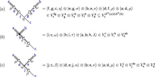
Figure 14: Diagrams for $\mathcal{S}^{2}\left(\mathsf{a}\right)\otimes\mathcal{S}^{2}\left(\mathsf{b}\right)$, $\mathcal{S}^{2}\left(\mathsf{a}\otimes\mathsf{b}\right)$ and $\mathcal{S}\left(\mathcal{S}\left(\mathsf{a}\right)\otimes\mathcal{S}\left(\mathsf{b}\right)\right)$. These diagrams are understood as vectors. (a) Diagram for $\mathcal{S}^{2}\left(\mathsf{a}\right)\otimes\mathcal{S}^{2}\left(\mathsf{b}\right)$. Different $\mathsf{d}$, $\mathsf{e}$, $\mathsf{f}$, $\mathsf{g}$, $\mu$, $\nu$, $\rho$, $\sigma$, and $\eta$ label different orthogonal vectors in the whole space $V_{\mathsf{c}}^{\mathcal{S}^{2}\left(\mathsf{a}\right)\otimes\mathcal{S}^{2}\left(\mathsf{b}\right)}$, which is isomorphic to $\oplus_{\mathsf{defg}}V_{\mathsf{c}}^{\mathsf{fg}}\otimes V_{\mathsf{g}}^{\mathsf{e}}\otimes V_{\mathsf{e}}^{\mathsf{b}}\otimes V_{\mathsf{f}}^{\mathsf{d}}\otimes V_{\mathsf{d}}^{\mathsf{a}}$. (b) Diagram for $\mathcal{S}^{2}\left(\mathsf{a}\otimes\mathsf{b}\right)$. Different $\mathsf{h}$, $\mathsf{i}$, $\lambda$, $\tau$, and $\omega$ label different orthogonal vectors. The tensor product construction in this diagram indicates that the whole space $V_{\mathsf{c}}^{\mathcal{S}^{2}\left(\mathsf{a}\right)\otimes\mathcal{S}^{2}\left(\mathsf{b}\right)}$ is isomorphic to $\oplus_{\mathsf{hi}}V_{\mathsf{c}}^{\mathsf{i}}\otimes V_{\mathsf{i}}^{\mathsf{h}}\otimes V_{\mathsf{h}}^{\mathsf{ab}}$. (c) Diagram for $\mathcal{S}\left(\mathcal{S}\left(\mathsf{a}\right)\otimes\mathcal{S}\left(\mathsf{b}\right)\right)$. Different $\mathsf{d}$, $\mathsf{e}$, $\mathsf{j}$, $\mu$, $\nu$, $\alpha$, and $\beta$ label different orthogonal vectors. The tensor product construction in this diagram indicates that the whole space is isomorphic to $\oplus_{\mathsf{dej}}V_{\mathsf{c}}^{\mathsf{j}}\otimes V_{\mathsf{j}}^{\mathsf{de}}\otimes V_{\mathsf{e}}^{\mathsf{b}}\otimes V_{\mathsf{d}}^{\mathsf{a}}$.

Now we consider using unitary matrices to change bases. Since generally $\mathcal{S}\left(\mathsf{a}\right)\otimes\mathcal{S}\left(\mathsf{b}\right)=\mathcal{S}\left(\mathsf{a}\otimes\mathsf{b}\right)$ does not hold for all excitations in $5$D, we need to introduce a new set of unitary matrices: $\Delta^{2}$-symbols as shown in figure 15, to transform from $\mathcal{S}^{2}\left(\mathsf{a}\right)\otimes\mathcal{S}^{2}\left(\mathsf{b}\right)$ to $\mathcal{S}^{2}\left(\mathsf{a}\otimes\mathsf{b}\right)$. Unitarity demands:

$$\sum_{\begin{subarray}{c}\mathsf{d},\mathsf{e},\mathsf{f},\mathsf{g},\\ \mu,\nu,\rho,\sigma,\eta\end{subarray}}{\left[{\Delta^{2}}_{\mathsf{c}}^{\mathsf{ab}}\right]_{\mathsf{defg}\mu\nu\rho\sigma\eta,\mathsf{hi}\lambda\tau\omega}\left(\left[{\Delta^{2}}_{\mathsf{c}}^{\mathsf{ab}}\right]_{\mathsf{defg}\mu\nu\rho\sigma\eta,\mathsf{h}^{\prime}\mathsf{i}^{\prime}\lambda^{\prime}\tau^{\prime}\omega^{\prime}}\right)^{\ast}}=\delta_{\mathsf{hh}^{\prime}}\delta_{\mathsf{ii}^{\prime}}\delta_{\lambda\lambda^{\prime}}\delta_{\tau\tau^{\prime}}\delta_{\omega\omega^{\prime}}\,,$$ (57)

$$\sum_{\mathsf{h},\mathsf{i},\lambda,\tau,\omega}{\left[{\Delta^{2}}_{\mathsf{c}}^{\mathsf{ab}}\right]_{\mathsf{defg}\mu\nu\rho\sigma\eta,\mathsf{hi}\lambda\tau\omega}\left(\left[{\Delta^{2}}_{\mathsf{c}}^{\mathsf{ab}}\right]_{\mathsf{d}^{\prime}\mathsf{e}^{\prime}\mathsf{f}^{\prime}\mathsf{g}^{\prime}\mu^{\prime}\nu^{\prime}\rho^{\prime}\sigma^{\prime}\eta^{\prime},\mathsf{hi}\lambda\tau\omega}\right)^{\ast}}=\delta_{\mathsf{dd}^{\prime}}\delta_{\mathsf{ee}^{\prime}}\delta_{\mathsf{ff}^{\prime}}\delta_{\mathsf{gg}^{\prime}}\delta_{\mu\mu^{\prime}}\delta_{\nu\nu^{\prime}}\delta_{\rho\rho^{\prime}}\delta_{\sigma\sigma^{\prime}}\delta_{\eta\eta^{\prime}}\,.$$ (58)

As for changing bases from $\mathcal{S}^{2}\left(\mathsf{a}\right)\otimes\mathcal{S}^{2}\left(\mathsf{b}\right)$ to $\mathcal{S}\left(\mathcal{S}\left(\mathsf{a}\right)\otimes\mathcal{S}\left(\mathsf{b}\right)\right)$, we can still use $\Delta$-symbols shown in figure 11 because even in $5$D, loops and particles still obey $\mathcal{S}\left(\mathsf{c}\right)\otimes\mathcal{S}\left(\mathsf{d}\right)=\mathcal{S}\left(\mathsf{c}\otimes\mathsf{d}\right)$. Thus, as shown in figure 16 and 17, we establish basis transformations between the three diagrams in figure 14.

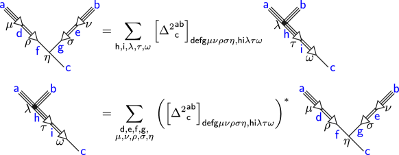
Figure 15: Definition of $\Delta^{2}$-symbols. The left and right diagrams describe the same physics in different bases. We can use a unitary $\Delta^{2}$-symbols to change bases.

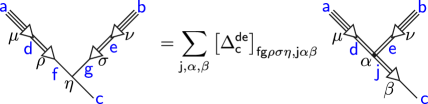
Figure 16: Basis transformation from $\mathcal{S}^{2}\left(\mathsf{a}\right)\otimes\mathcal{S}^{2}\left(\mathsf{b}\right)$ to $\mathcal{S}\left(\mathcal{S}\left(\mathsf{a}\right)\otimes\mathcal{S}\left(\mathsf{b}\right)\right)$. Since $\mathsf{d}$ and $\mathsf{e}$ can only be loops and particles, we are allowed to use the $\Delta$-symbol to change the basis.

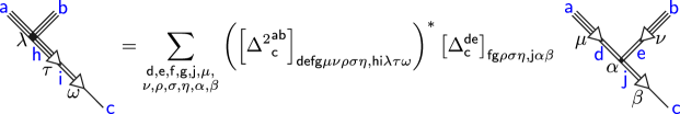
Figure 17: Basis transformation from $\mathcal{S}^{2}\left(\mathsf{a}\otimes\mathsf{b}\right)$ to $\mathcal{S}\left(\mathcal{S}\left(\mathsf{a}\right)\otimes\mathcal{S}\left(\mathsf{b}\right)\right)$. We can derive this transformation by using the lower diagram in figure 15 and then use figure 16.

V.3 Diagrammatic representations of the hierarchical shrinking-fusion hexagon equation

Before we go further to consider diagrams involving three excitations that go through shrinking and fusion processes, we draw figure 13 more compactly as shown in figure 18. We use a triangle with a line inside the triangle, in order to represent the whole hierarchical shrinking process. If we only consider using $\Delta^{2}$-symbols and $F$-symbols, it is convenient to use such a compact fashion to simplify our diagrams.

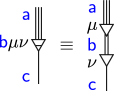
Figure 18: Hierarchical shrinking diagram in a more compact form. We draw the diagram on the left hand side as the simplified hierarchical shrinking diagram for the following discussion and physically there is nothing new. The triangle with a line represents the complete hierarchical shrinking process.

Recall the figure 12, we consider three excitations go through shrinking processes and fusion processes to finally get a particle. By using $F$-symbols and $\Delta$-symbols, we transform diagrams from each other and finally derive the shrinking-fusion hexagon equation in $4$D. We can now generalize it to $5$D through replacing $\Delta$-symbols and shrinking diagrams shown in figure 9 by $\Delta^{2}$-symbols and compact form hierarchical shrinking diagrams shown in figure 18 respectively. The resulting diagram shown in figure 19 gives the hierarchical shrinking-fusion hexagon equation in $5$D. The upper path and the lower path transform the far left diagram to the far right diagram differently. By comparing the coefficients of the far right diagram, we derive the hierarchical shrinking-fusion hexagon equation:

$$\sum_{\mathsf{i},\mathsf{q}}{\sum_{\alpha=1}^{N_{\mathsf{i}}^{\mathsf{fg}}}{\sum_{\beta=1}^{N_{\mathsf{d}}^{\mathsf{ei}}}{\sum_{\xi=1}^{\mathrm{S}_{\mathsf{q}}^{\mathsf{j}}}{\sum_{\psi=1}^{\mathrm{S}_{\mathsf{i}}^{\mathsf{q}}}{}}}}}\left[F_{\mathsf{d}}^{\mathsf{efg}}\right]_{\mathsf{h}\delta\gamma,\mathsf{i}\alpha\beta}\left[{\Delta^{2}}_{\mathsf{i}}^{\mathsf{bc}}\right]_{\mathsf{npfg}\nu\lambda\eta\phi\alpha,\mathsf{jq}\tau\xi\psi}\left[{\Delta^{2}}_{\mathsf{d}}^{\mathsf{aj}}\right]_{\mathsf{mqei}\mu\xi\chi\psi\beta,\mathsf{kr}\theta\epsilon\kappa}$$

$$= \sum_{\mathsf{t},\mathsf{s}}{\sum_{\sigma=1}^{N_{\mathsf{t}}^{\mathsf{ab}}}{\sum_{\omega=1}^{N_{\mathsf{k}}^{\mathsf{tc}}}{\sum_{\rho=1}^{\mathrm{S}_{\mathsf{s}}^{\mathsf{t}}}{\sum_{\zeta=1}^{\mathrm{S}_{\mathsf{h}}^{\mathsf{s}}}{}}}}}\left[{\Delta^{2}}_{\mathsf{h}}^{\mathsf{ab}}\right]_{\mathsf{mnef}\mu\nu\chi\eta\delta,\mathsf{ts}\sigma\rho\zeta}\left[{\Delta^{2}}_{\mathsf{d}}^{\mathsf{tc}}\right]_{\mathsf{sphg}\rho\lambda\zeta\phi\gamma,\mathsf{kr}\omega\epsilon\kappa}\left[F_{\mathsf{k}}^{\mathsf{abc}}\right]_{\mathsf{t}\sigma\omega,\mathsf{j}\tau\theta}\,.$$ (59)

Eq. (59) can be understood as the consistency relation between $F$-symbols and $\Delta^{2}$-symbols.

If we do not use the compact diagram in figure 18, we can consider using $\Delta$-symbols in figure 19, and we will find that shrinking-fusion hexagon (51) still holds, but now $\mathsf{a}$, $\mathsf{b}$ and $\mathsf{c}$ in eq. (51) can only be excitations listed in the subset $\Phi_{1}^{5}$. Such shrinking-fusion hexagon equation with a constraint on inputs is the consistency relation between $F$-symbols and $\Delta$-symbols in $5$D.

Eq. (59) and eq. (51) with constraint inputs are the key results in our $5$D diagrammatic representations, they establish the consistency relation between $F$-symbols, $\Delta$-symbols and $\Delta^{2}$-symbols. They also imply the constraint on fusion and shrinking coefficients, i.e., eq. (56). We conjecture that all anomaly-free $5$D topological orders should satisfy these two hexagon equations and thus have consistent fusion, shrinking, and hierarchical shrinking rules.

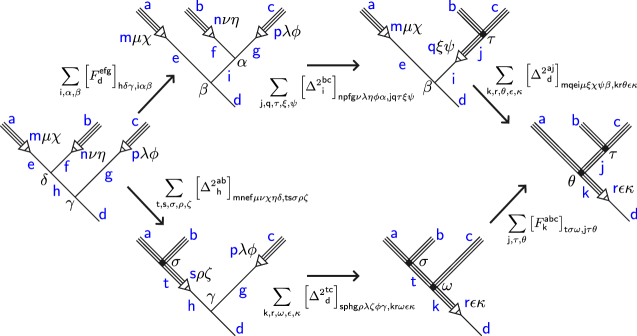
Figure 19: Diagrammatic representations of the hierarchical shrinking-fusion hexagon equation. Here we use simplified hierarchical shrinking diagrams shown in figure 18. Similar to figure 12, we have two different paths to transform the far left diagram to the far right diagram. Comparing these two different paths, we obtained the hierarchical shrinking-fusion hexagon equation.

VI Summary and outlook

In this paper, we have successfully constructed diagrammatic representations for higher-dimensional topological orders in 4D and 5D spacetimes, extending the framework known for 3D topologically ordered phases. By introducing and manipulating basic fusion and shrinking diagrams as vectors within corresponding spaces, we have demonstrated the construction of complex diagrams through their stacking. Using $F$-, $\Delta$-, and $\Delta^{2}$-symbols, we have established transformations between different bases in these vector spaces and derived key consistency conditions, including the pentagon equations and (hierarchical) shrinking-fusion hexagon equations. Our findings indicate that these consistency conditions are essential for ensuring the anomaly-free nature of higher-dimensional topological orders. Violations of these conditions suggest the presence of quantum anomalies, providing a diagnostic tool for identifying such anomalies in theoretical models.

Looking ahead, our work points towards several promising avenues for future research:

• In this paper, we solely focus on diagrams pertaining to fusion and shrinking rules, although it is worth noting that braiding statistics also hold significance in comprehending higher-dimensional topological orders. While diagrammatic representation of braiding processes is definitely intricate due to the involvement of spatially extended excitations, incorporating braiding processes into our diagrammatic representations presents an intriguing avenue for future exploration. Doing so may unveil new diagrammatic rules capable of encoding more complete algebraic structures relevant to braiding, fusion, and shrinking processes. Based on all data depicted by field theory and consistency conditions in diagrammatic representations, it is further interesting to study the connection between our field-theory-inspired diagrammatic representations and categorical approach in the future.

• $BF$ theory exhibits a close relationship with non-invertible symmetry and symmetry topological field theory (SymTFT). Various twisted terms, along with their fusion rules and braiding statistics, have been involved in the context of SymTFT, including notable examples such as $BB$, $BBA$, and $AdAdA$ twisted term, see, e.g., Refs. Kaidi et al. (2023b); Antinucci and Benini (2024); Brennan and Sun (2024); Argurio et al. (2024). It would be intriguing to explore the incorporation of shrinking and hierarchical shrinking rules into SymTFT and establish connections between SymTFT and our diagrammatic representations. Such investigations hold the potential to enrich our understanding of both SymTFT and the broader landscape of topological field theories.

• In this paper, our focus is primarily on the diagrammatic representations of $4$D and $5$D topological orders. However, it is worth noting that the framework we have developed lends itself to potential generalization for arbitrarily higher-dimensional topological orders. Such generalization holds promise for providing deeper insights into the underlying structure and properties of higher-dimensional topological orders, warranting further exploration in future studies.

Appendix A Review of anyon diagrams

In this appendix, we will briefly review the basic concepts in the diagrammatic representations of anyons. The diagrammatic rules and algebra set up the structure of anyon theories and they are closely related to TQFT descriptions.

A.1 Fusion rules and diagrammatic representations

Since shrinking rules are trivial in $3$D, we do not need to put excitations in different sets and treat them differently. Thus we can easily recover the diagrammatic representations for anyons by drawing all fusion diagrams in a single-line fashion.

Suppose the anyonic fusion process $\mathsf{a}\otimes\mathsf{b}$ has fusion channels to $\mathsf{c}$, we can represent this fusion process diagrammatically in figure 20. $\mu=\left\{1,2,\cdots,N_{\mathsf{c}}^{\mathsf{a}\mathsf{b}}\right\}$ labels different fusion channels to $\mathsf{c}$ and the diagram can be defined as a vector $\ket{\mathsf{a},\mathsf{b};\mathsf{c},\mu}$, different $\mu$ represent orthogonal vectors in the fusion space $V_{\mathsf{c}}^{\mathsf{a}\mathsf{b}}$ with $\text{dim}(V_{\mathsf{c}}^{\mathsf{a}\mathsf{b}})=N_{\mathsf{c}}^{\mathsf{a}\mathsf{b}}$. For fusing three anyons, suppose $\left(\mathsf{a}\otimes\mathsf{b}\right)\otimes\mathsf{c}$ has fusion channels to $\mathsf{d}$, diagrammatically we have the upper diagram shown in figure 21. Associativity indicates that the upper and the lower diagrams in figure 21 represent different bases and we can use a unitary $F$-symbol to change the basis. The definition of $F$-symbol is given by figure 22.

Figure 20: Fusion diagram of two anyons. $\mathsf{a}$, $\mathsf{b}$ and $\mathsf{c}$ denote anyons, $\mu=\left\{1,2,\cdots,N_{\mathsf{c}}^{\mathsf{a}\mathsf{b}}\right\}$ labels different fusion channels to $\mathsf{c}$.

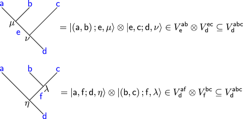
Figure 21: Fusion diagram of three anyons. $\mathsf{a}$, $\mathsf{b}$, and $\mathsf{c}$ are input anyons and they finally fuse to $\mathsf{d}$. The anyons in the bracket fuse together first. $\otimes$ mean tensor product here. In the upper diagram, the set $\left\{\ket{\left(\mathsf{a},\mathsf{b}\right);\mathsf{e},\mu}\otimes\ket{\mathsf{e},\mathsf{c};\mathsf{d},\nu}\right\}$ spans the whole space $V_{\mathsf{d}}^{\mathsf{abc}}$, different $\mu$, $\nu$ and $\mathsf{e}$ label different orthogonal vectors. Such space $V_{\mathsf{d}}^{\mathsf{abc}}$ is isomorphic to $\oplus_{\mathsf{e}}V_{\mathsf{e}}^{\mathsf{ab}}\otimes V_{\mathsf{d}}^{\mathsf{ec}}$ and thus $\text{dim}(V_{\mathsf{d}}^{\mathsf{a}\mathsf{b}\mathsf{c}})=\sum_{\mathsf{e}}{N_{\mathsf{e}}^{\mathsf{ab}}}N_{\mathsf{d}}^{\mathsf{ec}}$. For the lower diagram, the case is similar and we have $V_{\mathsf{d}}^{\mathsf{abc}}\cong\oplus_{\mathsf{f}}V_{\mathsf{d}}^{\mathsf{af}}\otimes V_{\mathsf{f}}^{\mathsf{bc}}$ and thus $\text{dim}(V_{\mathsf{d}}^{\mathsf{a}\mathsf{b}\mathsf{c}})=\sum_{\mathsf{f}}{N_{\mathsf{d}}^{\mathsf{af}}}N_{\mathsf{f}}^{\mathsf{bc}}=\sum_{\mathsf{e}}{N_{\mathsf{e}}^{\mathsf{ab}}}N_{\mathsf{d}}^{\mathsf{ec}}$.

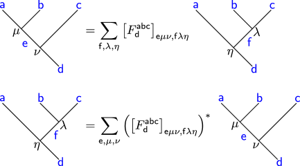
Figure 22: Definition of $F$-symbol. The left and right diagrams describe the same physics in different bases. We use unitary $F$-symbol to change the basis.

For other diagrams involving four anyons, as shown in figure 23, we use $F$-symbols to transform diagrams and derive the pentagon equation:

$$\sum_{\sigma=1}^{N_{\mathsf{e}}^{\mathsf{fh}}}{\left[F_{\mathsf{e}}^{\mathsf{fcd}}\right]_{\mathsf{g}\nu\lambda,\mathsf{h}\gamma\sigma}}\left[F_{\mathsf{e}}^{\mathsf{abh}}\right]_{\mathsf{f}\mu\sigma,\mathsf{i}\rho\delta}=\sum_{\mathsf{j}}{\sum_{\omega=1}^{N_{\mathsf{g}}^{\mathsf{aj}}}{\sum_{\theta=1}^{N_{\mathsf{j}}^{\mathsf{bc}}}{\sum_{\tau=1}^{N_{\mathsf{i}}^{\mathsf{jd}}}{\left[F_{\mathsf{g}}^{\mathsf{abc}}\right]_{\mathsf{f}\mu\nu,\mathsf{j}\theta\omega}\left[F_{\mathsf{e}}^{\mathsf{ajd}}\right]_{\mathsf{g}\omega\lambda,\mathsf{i}\tau\delta}\left[F_{\mathsf{i}}^{\mathsf{bcd}}\right]_{\mathsf{j}\theta\tau,\mathsf{h}\gamma\rho}}}}}\,.$$ (60)

No more identities beyond the pentagon equation can be derived by drawing more complicated fusion diagrams. A set of unitary $F$-symbols satisfying the pentagon equation form a unitary fusion category.

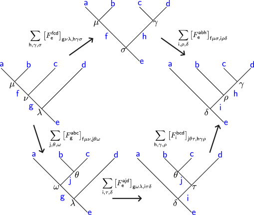
Figure 23: Pentagon equation. We use blue to highlight the anyons. Starting from the far left diagram, we can go to the far right diagram through either the upper path or the lower path. Comparing these two different paths, we can derive the pentagon equation.

A.2 Braiding statistics and diagrammatic representations

In section A.1, we only consider fusion processes, thus worldlines will not cross each other. In this section, we allow worldlines to cross over and under each other to form braiding processes. For Abelian anyons, a braiding process only accumulates a phase $e^{i\theta}$, which can be regarded as a one-dimensional representation of the braid group. However, for non-Abelian anyons, a braiding process is equivalent to multiplying a unitary matrix to the initial wavefunction of the system. This unitary matrix can be regarded as a higher-dimensional representation of the braid group.

Suppose $\mathsf{a}$ and $\mathsf{b}$ fuse to $\mathsf{c}$, then this process can be viewed as a vector in fusion space $V^{\mathsf{ab}}_{\mathsf{c}}$. Due to the principle of locality, if we (half) braid $\mathsf{a}$ and $\mathsf{b}$ first and then fuse them together, the fusion output is still $\mathsf{c}$, and thus this whole process can also be viewed as a vector in space $V^{\mathsf{ab}}_{\mathsf{c}}$. These two vectors are related to each other through the $R$-symbol, as shown in figure 24. The left and right hand sides of figure 24 correspond to under-crossing and over-crossing respectively. $\left[R_{\mathsf{c}}^{\mathsf{ba}}\right]^{-1}$ is the inverse of $\left[R_{\mathsf{c}}^{\mathsf{ba}}\right]$. Similar to $F$-symbol, $R$-symbol is also unitary:

$$\sum_{\nu}{\left[R_{\mathsf{c}}^{\mathsf{ab}}\right]_{\mu,\nu}}\left(\left[R_{\mathsf{c}}^{\mathsf{ab}}\right]_{\mu^{\prime},\nu}\right)^{\ast}=\delta_{\mu\mu^{\prime}}\,.$$ (61)

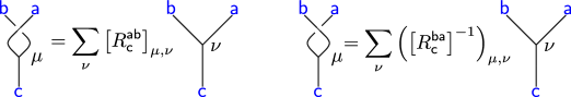
Figure 24: Definition of $R$-symbol. The left and right hand sides correspond to under-crossing and over-crossing respectively. $-1$ denotes the inverse matrix. Since $R$-symbol is unitary, $\left(\left[R_{\mathsf{c}}^{\mathsf{ba}}\right]^{-1}\right)_{\mu,\nu}$ can be written as $\left(\left[R_{\mathsf{c}}^{\mathsf{ba}}\right]_{\nu,\mu}\right)^{\ast}$.

Consider using $F$-symbols and $R$-symbols in diagrams involving three anyons, as shown in figure 25, we can derive consistency relations for $F$-symbols and $R$-symbols in $3$D topological order, known as hexagon equations:

$$\sum_{\lambda}^{N_{\mathsf{e}}^{\mathsf{ac}}}{\sum_{\eta}^{N_{\mathsf{f}}^{\mathsf{cb}}}{\left[R_{\mathsf{e}}^{\mathsf{ca}}\right]_{\mu,\lambda}\left[F_{\mathsf{d}}^{\mathsf{acb}}\right]_{\mathsf{e}\lambda\nu,\mathsf{f}\eta\tau}\left[R_{\mathsf{f}}^{\mathsf{cb}}\right]_{\eta,\gamma}}}$$

$$= \sum_{\mathsf{g}}{\sum_{\rho}^{N_{\mathsf{g}}^{\mathsf{ab}}}{\sum_{\sigma}^{N_{\mathsf{d}}^{\mathsf{cg}}}{\sum_{\omega}^{N_{\mathsf{d}}^{\mathsf{gc}}}{\left[F_{\mathsf{d}}^{\mathsf{cab}}\right]_{\mathsf{e}\mu\nu,\mathsf{g}\rho\sigma}\left[R_{\mathsf{d}}^{\mathsf{cg}}\right]_{\sigma,\omega}\left[F_{\mathsf{d}}^{\mathsf{abc}}\right]_{\mathsf{g}\rho\omega,\mathsf{f}\gamma\tau}}}}}\,,$$ (62)

$$\sum_{\lambda}^{N_{\mathsf{e}}^{\mathsf{ac}}}{\sum_{\eta}^{N_{\mathsf{f}}^{\mathsf{cb}}}{\left(\left[R_{\mathsf{e}}^{\mathsf{ac}}\right]^{-1}\right)_{\mu,\lambda}\left[F_{\mathsf{d}}^{\mathsf{acb}}\right]_{\mathsf{e}\lambda\nu,\mathsf{f}\eta\tau}\left(\left[R_{\mathsf{f}}^{\mathsf{bc}}\right]^{-1}\right)_{\eta,\gamma}}}$$

$$= \sum_{\mathsf{g}}{\sum_{\rho}^{N_{\mathsf{g}}^{\mathsf{ab}}}{\sum_{\sigma}^{N_{\mathsf{d}}^{\mathsf{cg}}}{\sum_{\omega}^{N_{\mathsf{d}}^{\mathsf{gc}}}{\left[F_{\mathsf{d}}^{\mathsf{cab}}\right]_{\mathsf{e}\mu\nu,\mathsf{g}\rho\sigma}\left(\left[R_{\mathsf{d}}^{\mathsf{gc}}\right]^{-1}\right)_{\sigma,\omega}\left[F_{\mathsf{d}}^{\mathsf{abc}}\right]_{\mathsf{g}\rho\omega,\mathsf{f}\gamma\tau}}}}}\,.$$ (63)

Eq. (62) and eq. (63) correspond to the upper and the lower diagrams in figure 25 respectively. A set of unitary $F$-symbols and unitary $R$-symbols satisfying pentagon and hexagon equations form a unitary braided tensor category, all $3$D anyon theories must be in this form. Given all fusion rules, there are only finite gauge inequivalent solutions of pentagon and hexagon equations.

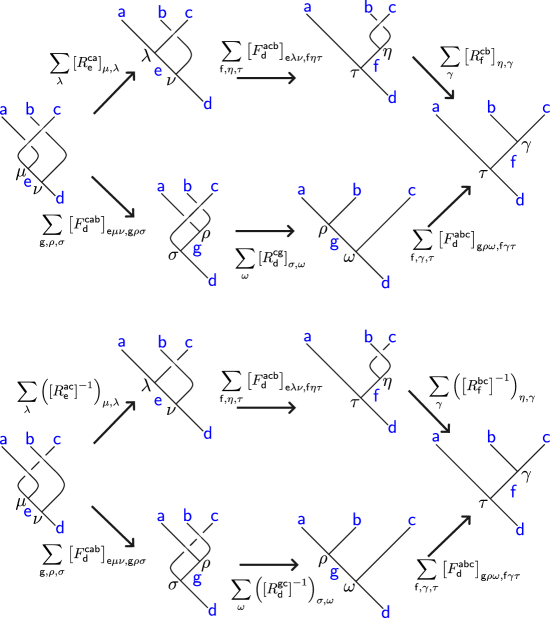
Figure 25: Hexagon equations. We use red and blue to highlight the matrices and anyons respectively. Eq. (62) and eq. (63) correspond to the upper (over-crossing) and the lower (under-crossing) hexagon diagrams. Similar to figure 23, for each hexagon diagram, we have two paths to transform the far left to the far right, comparing the upper and the lower paths directly leads to eq. (62) and eq. (63).

Appendix B Diagrams involving four excitations

In this appendix, we consider diagrams that involve four excitations and show that we cannot obtain new consistency relations besides pentagon and shrinking-fusion hexagon equations from these diagrams.

Starting with $\left[\left[\mathcal{S}\left(\mathsf{a}\right)\otimes\mathcal{S}\left(\mathsf{b}\right)\right]\otimes\mathcal{S}\left(\mathsf{c}\right)\right]\otimes\mathcal{S}\left(\mathsf{d}\right)$, we can finally generate a total of $21$ distinct diagrams by utilizing $F$- and $\Delta$-symbols. We list all these diagrams in figure 26 and omit all excitation and channel labels for simplicity. The relations between these $21$ diagrams are shown in figure 27, where we use arrows with $F$ or $\Delta$ to indicate transformations via $F$- or $\Delta$-symbols. From figure 27 we can find $13$ candidates for independent polygon equations as shown in figure 28. However, upon recovering the excitation and channel labels and attempting to write down the consistent equations, we find that only pentagon and shrinking-fusion hexagon equations are independent while other equations are automatically satisfied and thus trivial.

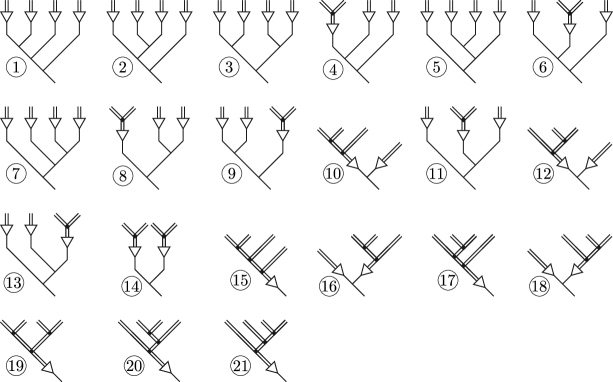
Figure 26: All $21$ diagrams that involve four topological excitations. We label them from $1$ to $21$ and their relations are given in figure 27.

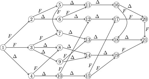
Figure 27: The relations between the $21$ diagrams. An arrow with $F$ or $\Delta$ means that we can use $F$- or $\Delta$-symbols to transform the diagram. For example, diagram $1$ can be transform to diagram $3$ by using an $F$-symbol, diagram $3$ can be transform to diagram $9$ by using a $\Delta$-symbol.

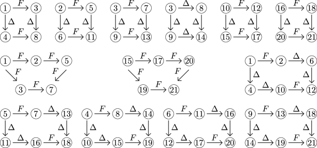
Figure 28: $13$ polygons from figure 27. It turns out that all quadrilateral equations are trivial. Pentagons and hexagons essentially give independent pentagon and shrinking-fusion hexagon equations.

To be more specific, we consider the quadrilateral equation given by diagrams $1$, $3$, $4$, and $8$ as an example. The transformations $1\rightarrow 3\rightarrow 8$ and $1\rightarrow 3\rightarrow 4$ gives coefficients

$$1\rightarrow 3\rightarrow 8:\quad\sum_{\mathsf{m},\gamma,\eta}{\sum_{\mathsf{n},\delta,\tau}{\left[F_{\mathsf{k}}^{\mathsf{igh}}\right]_{\mathsf{j}\sigma\lambda,\mathsf{m}\gamma\eta}\left[\Delta_{\mathsf{i}}^{\mathsf{ab}}\right]_{\mathsf{ef}\mu\nu\rho,\mathsf{n}\delta\tau}}}$$

$$1\rightarrow 4\rightarrow 8:\quad\sum_{\mathsf{n},\delta,\tau}{\sum_{\mathsf{m},\gamma,\eta}{\left[\Delta_{\mathsf{i}}^{\mathsf{ab}}\right]_{\mathsf{ef}\mu\nu\rho,\mathsf{n}\delta\tau}\left[F_{\mathsf{k}}^{\mathsf{igh}}\right]_{\mathsf{j}\sigma\lambda,\mathsf{m}\gamma\eta}}}$$

respectively. We can see that they equal to each other automatically and thus the quadrilateral equation is trivial. For a similar reason, other quadrilateral equations are also trivial. The two pentagons in figure 28 respectively give pentagon equations for $\left\{\mathsf{a},\mathsf{b},\mathsf{c},\mathsf{d}\right\}$ and $\left\{\mathcal{S}\left(\mathsf{a}\right),\mathcal{S}\left(\mathsf{b}\right),\mathcal{S}\left(\mathsf{c}\right),\mathcal{S}\left(\mathsf{d}\right)\right\}$, $\mathsf{a},\mathsf{b},\mathsf{c},\mathsf{d}\in\Phi_{0}^{4}$. Since $\mathcal{S}\left(\mathsf{a}\right),\mathcal{S}\left(\mathsf{b}\right),\mathcal{S}\left(\mathsf{c}\right),\mathcal{S}\left(\mathsf{d}\right)\in\Phi_{1}^{4}\subseteq\Phi_{0}^{4}$, the later pentagon equation is automatically satisfied when we demand that the former pentagon equation holds. The $5$ hexagons shown in figure 28 respectively give hexagon equations for $\left\{\mathsf{a},\mathsf{b},\mathsf{c}\right\}$, $\left\{\mathsf{b},\mathsf{c},\mathsf{d}\right\}$, $\left\{\left(\mathsf{a}\otimes\mathsf{b}\right),\mathsf{c},\mathsf{d}\right\}$, $\left\{\mathsf{a},\left(\mathsf{b}\otimes\mathsf{c}\right),\mathsf{d}\right\}$ and $\left\{\mathsf{a},\mathsf{b},\left(\mathsf{c}\otimes\mathsf{d}\right)\right\}$ respectively and essential they are the same equation. Thus we conclude that there are only two independent equations in figure 28, which are pentagon and shrinking-fusion hexagon equations.

References

- Zeng et al. (2018) Bei Zeng, Xie Chen, Duan-Lu Zhou, and Xiao-Gang Wen, “Quantum information meets quantum matter – from quantum entanglement to topological phase in many-body systems,” (2018), arXiv:1508.02595 [cond-mat.str-el] .
- Wen (2017) Xiao-Gang Wen, “Colloquium: Zoo of quantum-topological phases of matter,” Rev. Mod. Phys. 89, 041004 (2017).
- Witten (1989) Edward Witten, “Quantum field theory and the jones polynomial,” Commun. Math. Phys. 121, 351–399 (1989).
- Turaev (2016) Vladimir G. Turaev, Quantum Invariants of Knots and 3-Manifolds (De Gruyter, Berlin, Boston, 2016).
- Blok and Wen (1990) B. Blok and X. G. Wen, “Effective theories of the fractional quantum hall effect at generic filling fractions,” Phys. Rev. B 42, 8133–8144 (1990).
- Nayak" (2008) Chetan Nayak", “Non-abelian anyons and topological quantum computation,” Reviews of Modern Physics 80, 1083–1159 (2008).
- Wen (2004) Xiao-Gang Wen, Quantum field theory of many-body systems: from the origin of sound to an origin of light and electrons (Oxford University Press, 2004).
- Lu and Vishwanath (2012) Yuan-Ming Lu and Ashvin Vishwanath, “Theory and classification of interacting integer topological phases in two dimensions: A chern-simons approach,” Phys. Rev. B 86, 125119 (2012).
- Ye and Wen (2013) Peng Ye and Xiao-Gang Wen, “Projective construction of two-dimensional symmetry-protected topological phases with u(1), so(3), or su(2) symmetries,” Phys. Rev. B 87, 195128 (2013).
- Gu et al. (2016) Zheng-Cheng Gu, Juven C. Wang, and Xiao-Gang Wen, “Multikink topological terms and charge-binding domain-wall condensation induced symmetry-protected topological states: Beyond chern-simons/bf field theories,” Phys. Rev. B 93, 115136 (2016).
- Hung and Wan (2013) Ling-Yan Hung and Yidun Wan, “ matrix construction of symmetry-enriched phases of matter,” Phys. Rev. B 87, 195103 (2013).
- Kitaev (2006) Alexei Kitaev, “Anyons in an exactly solved model and beyond,” Annals of Physics 321, 2–111 (2006), january Special Issue.
- Levin and Wen (2005) Michael A. Levin and Xiao-Gang Wen, “String-net condensation: A physical mechanism for topological phases,” Phys. Rev. B 71, 045110 (2005).
- Chen et al. (2010) Xie Chen, Zheng-Cheng Gu, and Xiao-Gang Wen, “Local unitary transformation, long-range quantum entanglement, wave function renormalization, and topological order,” Phys. Rev. B 82, 155138 (2010).
- Bonderson (2007) Parsa Hassan. Bonderson, Non-Abelian Anyons and Interferometry., Ph.D. thesis, California Institute of Technology. (2007).
- Ardonne and Slingerland (2010) Eddy Ardonne and Joost Slingerland, “Clebsch-gordan and 6j-coefficients for rank 2 quantum groups,” Journal of Physics A: Mathematical and Theoretical 43, 395205 (2010).
- Bonderson et al. (2008) Parsa Bonderson, Kirill Shtengel, and J.K. Slingerland, “Interferometry of non-abelian anyons,” Annals of Physics 323, 2709–2755 (2008).
- Eliëns et al. (2014) I. S. Eliëns, J. C. Romers, and F. A. Bais, “Diagrammatics for bose condensation in anyon theories,” Phys. Rev. B 90, 195130 (2014).
- Simon (2023) Steven H Simon, Topological quantum (Oxford University Press, 2023).
- Kong and Wen (2014) Liang Kong and Xiao-Gang Wen, “Braided fusion categories, gravitational anomalies, and the mathematical framework for topological orders in any dimensions,” (2014), arXiv:1405.5858 [cond-mat.str-el] .
- Barkeshli et al. (2019) Maissam Barkeshli, Parsa Bonderson, Meng Cheng, and Zhenghan Wang, “Symmetry fractionalization, defects, and gauging of topological phases,” Phys. Rev. B 100, 115147 (2019).
- Leinaas and Myrheim (1977) J. M. Leinaas and J. Myrheim, “On the theory of identical particles,” Il Nuovo Cimento B (1971-1996) 37, 1–23 (1977).
- Wu (1984) Yong-Shi Wu, “General theory for quantum statistics in two dimensions,” Phys. Rev. Lett. 52, 2103–2106 (1984).
- Alford and Wilczek (1989) M. G. Alford and Frank Wilczek, “Aharonov-bohm interaction of cosmic strings with matter,” Phys. Rev. Lett. 62, 1071–1074 (1989).
- Krauss and Wilczek (1989) Lawrence M. Krauss and Frank Wilczek, “Discrete gauge symmetry in continuum theories,” Phys. Rev. Lett. 62, 1221–1223 (1989).
- Wilczek and Zee (1983) Frank Wilczek and A. Zee, “Linking numbers, spin, and statistics of solitons,” Phys. Rev. Lett. 51, 2250–2252 (1983).
- Goldhaber et al. (1989) Alfred S Goldhaber, R MacKenzie, and Frank Wilczek, “Field corrections to induced statistics,” Mod. Phys. Lett. A 4, 21–31 (1989).
- Horowitz and Srednicki (1990) Gary T. Horowitz and Mark Srednicki, “A quantum field theoretic description of linking numbers and their generalization,” Commun.Math. Phys. 130, 83–94 (1990).
- Ye et al. (2016) Peng Ye, Taylor L. Hughes, Joseph Maciejko, and Eduardo Fradkin, “Composite particle theory of three-dimensional gapped fermionic phases: Fractional topological insulators and charge-loop excitation symmetry,” Phys. Rev. B 94, 115104 (2016).
- Moy et al. (2023) Benjamin Moy, Hart Goldman, Ramanjit Sohal, and Eduardo Fradkin, “Theory of oblique topological insulators,” SciPost Phys. 14, 023 (2023).
- Ye and Wen (2014) Peng Ye and Xiao-Gang Wen, “Constructing symmetric topological phases of bosons in three dimensions via fermionic projective construction and dyon condensation,” Phys. Rev. B 89, 045127 (2014).
- Putrov et al. (2017) Pavel Putrov, Juven Wang, and Shing-Tung Yau, “Braiding statistics and link invariants of bosonic/fermionic topological quantum matter in 2+1 and 3+1 dimensions,” Annals of Physics 384, 254 – 287 (2017).
- Wang et al. (2019) Qing-Rui Wang, Meng Cheng, Chenjie Wang, and Zheng-Cheng Gu, “Topological quantum field theory for abelian topological phases and loop braiding statistics in -dimensions,” Phys. Rev. B 99, 235137 (2019).
- Ye and Gu (2016) Peng Ye and Zheng-Cheng Gu, “Topological quantum field theory of three-dimensional bosonic abelian-symmetry-protected topological phases,” Phys. Rev. B 93, 205157 (2016).
- Wen et al. (2018) Xueda Wen, Huan He, Apoorv Tiwari, Yunqin Zheng, and Peng Ye, “Entanglement entropy for (3+1)-dimensional topological order with excitations,” Phys. Rev. B 97, 085147 (2018).
- Chan et al. (2018) AtMa P. O. Chan, Peng Ye, and Shinsei Ryu, “Braiding with borromean rings in ()-dimensional spacetime,” Phys. Rev. Lett. 121, 061601 (2018).
- Zhang and Ye (2021) Zhi-Feng Zhang and Peng Ye, “Compatible braidings with Hopf links, multi-loop, and Borromean rings in (3+1)-dimensional spacetime,” Phys. Rev. Research 3, 023132 (2021).
- Ye and Gu (2015) Peng Ye and Zheng-Cheng Gu, “Vortex-line condensation in three dimensions: A physical mechanism for bosonic topological insulators,” Phys. Rev. X 5, 021029 (2015).
- Ye and Wang (2013) Peng Ye and Juven Wang, “Symmetry-protected topological phases with charge and spin symmetries: Response theory and dynamical gauge theory in two and three dimensions,” Phys. Rev. B 88, 235109 (2013).
- Schafer-Nameki (2023) Sakura Schafer-Nameki, “Ictp lectures on (non-)invertible generalized symmetries,” (2023), arXiv:2305.18296 [hep-th] .
- Heidenreich et al. (2021) Ben Heidenreich, Jacob McNamara, Miguel Montero, Matthew Reece, Tom Rudelius, and Irene Valenzuela, “Non-invertible global symmetries and completeness of the spectrum,” Journal of High Energy Physics 2021, 203 (2021), arXiv:2104.07036 [hep-th] .
- Kaidi et al. (2022) Justin Kaidi, Kantaro Ohmori, and Yunqin Zheng, “Kramers-wannier-like duality defects in gauge theories,” Phys. Rev. Lett. 128, 111601 (2022).
- Choi et al. (2022) Yichul Choi, Clay Córdova, Po-Shen Hsin, Ho Tat Lam, and Shu-Heng Shao, “Noninvertible duality defects in dimensions,” Phys. Rev. D 105, 125016 (2022).
- Roumpedakis et al. (2023) Konstantinos Roumpedakis, Sahand Seifnashri, and Shu-Heng Shao, “Higher Gauging and Non-invertible Condensation Defects,” Communications in Mathematical Physics 401, 3043–3107 (2023), arXiv:2204.02407 [hep-th] .
- Kaidi et al. (2022) Justin Kaidi, Gabi Zafrir, and Yunqin Zheng, “Non-invertible symmetries of N = 4 SYM and twisted compactification,” Journal of High Energy Physics 2022, 53 (2022), arXiv:2205.01104 [hep-th] .
- Kaidi et al. (2023a) Justin Kaidi, Kantaro Ohmori, and Yunqin Zheng, “Symmetry TFTs for Non-invertible Defects,” Communications in Mathematical Physics 404, 1021–1124 (2023a), arXiv:2209.11062 [hep-th] .
- Kaidi et al. (2023b) Justin Kaidi, Emily Nardoni, Gabi Zafrir, and Yunqin Zheng, “Symmetry TFTs and anomalies of non-invertible symmetries,” Journal of High Energy Physics 2023, 53 (2023b), arXiv:2301.07112 [hep-th] .
- Choi et al. (2023) Yichul Choi, Clay Córdova, Po-Shen Hsin, Ho Tat Lam, and Shu-Heng Shao, “Non-invertible Condensation, Duality, and Triality Defects in 3+1 Dimensions,” Communications in Mathematical Physics 402, 489–542 (2023), arXiv:2204.09025 [hep-th] .
- Antinucci and Benini (2024) Andrea Antinucci and Francesco Benini, “Anomalies and gauging of u(1) symmetries,” (2024), arXiv:2401.10165 [hep-th] .
- Damia et al. (2023) Jeremias Aguilera Damia, Riccardo Argurio, and Eduardo Garcia-Valdecasas, “Non-invertible defects in 5d, boundaries and holography,” SciPost Phys. 14, 067 (2023).
- Argurio et al. (2024) Riccardo Argurio, Francesco Benini, Matteo Bertolini, Giovanni Galati, and Pierluigi Niro, “On the symmetry tft of yang-mills-chern-simons theory,” (2024), arXiv:2404.06601 [hep-th] .
- Cao and Jia (2024) Weiguang Cao and Qiang Jia, “Symmetry tft for subsystem symmetry,” (2024), arXiv:2310.01474 [hep-th] .
- Brennan and Sun (2024) T. Daniel Brennan and Zhengdi Sun, “A symtft for continuous symmetries,” (2024), arXiv:2401.06128 [hep-th] .
- Hansson et al. (2004) T.H. Hansson, Vadim Oganesyan, and S.L. Sondhi, “Superconductors are topologically ordered,” Annals of Physics 313, 497–538 (2004).
- Preskill and Krauss (1990) John Preskill and Lawrence M. Krauss, “Local discrete symmetry and quantum-mechanical hair,” Nuclear Physics B 341, 50 – 100 (1990).
- Alford et al. (1992) Mark G. Alford, Kai-Ming Lee, John March-Russell, and John Preskill, “Quantum field theory of non-abelian strings and vortices,” Nuclear Physics B 384, 251 – 317 (1992).
- Wang and Levin (2014) Chenjie Wang and Michael Levin, “Braiding statistics of loop excitations in three dimensions,” Phys. Rev. Lett. 113, 080403 (2014).
- Wang et al. (2015) Juven C. Wang, Zheng-Cheng Gu, and Xiao-Gang Wen, “Field-theory representation of gauge-gravity symmetry-protected topological invariants, group cohomology, and beyond,” Phys. Rev. Lett. 114, 031601 (2015).
- Wang and Wen (2015) Juven C. Wang and Xiao-Gang Wen, “Non-abelian string and particle braiding in topological order: Modular representation and -dimensional twisted gauge theory,” Phys. Rev. B 91, 035134 (2015).
- Jian and Qi (2014) Chao-Ming Jian and Xiao-Liang Qi, “Layer construction of 3d topological states and string braiding statistics,” Phys. Rev. X 4, 041043 (2014).
- Jiang et al. (2014) Shenghan Jiang, Andrej Mesaros, and Ying Ran, “Generalized modular transformations in topologically ordered phases and triple linking invariant of loop braiding,” Phys. Rev. X 4, 031048 (2014).
- Wang et al. (2016) Chenjie Wang, Chien-Hung Lin, and Michael Levin, “Bulk-boundary correspondence for three-dimensional symmetry-protected topological phases,” Phys. Rev. X 6, 021015 (2016).
- Tiwari et al. (2017) Apoorv Tiwari, Xiao Chen, and Shinsei Ryu, “Wilson operator algebras and ground states of coupled theories,” Phys. Rev. B 95, 245124 (2017).
- Kapustin and Thorngren (2014) A. Kapustin and R. Thorngren, “Anomalies of discrete symmetries in various dimensions and group cohomology,” ArXiv e-prints (2014), arXiv:1404.3230 [hep-th] .
- Wan et al. (2015) Yidun Wan, Juven C. Wang, and Huan He, “Twisted gauge theory model of topological phases in three dimensions,” Phys. Rev. B 92, 045101 (2015).
- Chen et al. (2016) Xiao Chen, Apoorv Tiwari, and Shinsei Ryu, “Bulk-boundary correspondence in (3+1)-dimensional topological phases,” Phys. Rev. B 94, 045113 (2016).
- Kapustin and Seiberg (2014) Anton Kapustin and Nathan Seiberg, “Coupling a QFT to a TQFT and Duality,” JHEP 04, 001 (2014), arXiv:1401.0740 [hep-th] .
- Zhang et al. (2023a) Zhi-Feng Zhang, Qing-Rui Wang, and Peng Ye, “Continuum field theory of three-dimensional topological orders with emergent fermions and braiding statistics,” Phys. Rev. Res. 5, 043111 (2023a).
- Qi and Zhang (2011) Xiao-Liang Qi and Shou-Cheng Zhang, “Topological insulators and superconductors,” Rev. Mod. Phys. 83, 1057–1110 (2011).
- Lapa et al. (2017) Matthew F. Lapa, Chao-Ming Jian, Peng Ye, and Taylor L. Hughes, “Topological electromagnetic responses of bosonic quantum hall, topological insulator, and chiral semimetal phases in all dimensions,” Phys. Rev. B 95, 035149 (2017).
- Ye et al. (2017) Peng Ye, Meng Cheng, and Eduardo Fradkin, “Fractional -duality, classification of fractional topological insulators, and surface topological order,” Phys. Rev. B 96, 085125 (2017).
- Witten (2016) Edward Witten, “Fermion path integrals and topological phases,” Rev. Mod. Phys. 88, 035001 (2016).
- Han et al. (2019) Bo Han, Huajia Wang, and Peng Ye, “Generalized wen-zee terms,” Phys. Rev. B 99, 205120 (2019).
- Zhang et al. (2023b) Zhi-Feng Zhang, Qing-Rui Wang, and Peng Ye, “Non-abelian fusion, shrinking, and quantum dimensions of abelian gauge fluxes,” Phys. Rev. B 107, 165117 (2023b).
- Ning et al. (2022) Shang-Qiang Ning, Zheng-Xin Liu, and Peng Ye, “Fractionalizing global symmetry on looplike topological excitations,” Phys. Rev. B 105, 205137 (2022).
- Ning et al. (2016) Shang-Qiang Ning, Zheng-Xin Liu, and Peng Ye, “Symmetry enrichment in three-dimensional topological phases,” Phys. Rev. B 94, 245120 (2016).
- Ye (2018) Peng Ye, “Three-dimensional anomalous twisted gauge theories with global symmetry: Implications for quantum spin liquids,” Phys. Rev. B 97, 125127 (2018).
- Zhang and Ye (2022) Zhi-Feng Zhang and Peng Ye, “Topological orders, braiding statistics, and mixture of two types of twisted BF theories in five dimensions,” J. High Energ. Phys. 2022, 138 (2022).
- Huang et al. (2023) Yizhou Huang, Zhi-Feng Zhang, and Peng Ye, “Fusion rules and shrinking rules of topological orders in five dimensions,” JHEP 11, 210 (2023), arXiv:2306.14611 [hep-th] .