New Perspectives on the Optimal Placement of Detectors for Suicide Bombers using Metaheuristics

Abstract

We consider an operational model of suicide bombing attacks –an increasingly prevalent form of terrorism– against specific targets, and the use of protective countermeasures based on the deployment of detectors over the area under threat. These detectors have to be carefully located in order to minimize the expected number of casualties or the economic damage suffered, resulting in a hard optimization problem for which different metaheuristics have been proposed. Rather than assuming random decisions by the attacker, the problem is approached by considering different models of the latter, whereby he takes informed decisions on which objective must be targeted and through which path it has to be reached based on knowledge on the importance or value of the objectives or on the defensive strategy of the defender (a scenario that can be regarded as an adversarial game). We consider four different algorithms, namely a greedy heuristic, a hill climber, tabu search and an evolutionary algorithm, and study their performance on a broad collection of problem instances trying to resemble different realistic settings such as a coastal area, a modern urban area, and the historic core of an old town. It is shown that the adversarial scenario is harder for all techniques, and that the evolutionary algorithm seems to adapt better to the complexity of the resulting search landscape.

1 Introduction

The threat of international terrorism has been present for many decades now, but ever since the collapse of the Eastern bloc in the late 1980s and the subsequent end of the Cold War it has emerged as the major factor of instability and social disruption at a global scale, be it directly as a consequence of terrorist actions or indirectly as a result of the countermeasures required to prevent the former and the impact of these in our daily lives (not to mention the military operations targeting terrorist groups and regimes supporting them, which in themselves contribute both to local turmoil and social unrest). Indeed, the new international environment arising from the end of the Atlantic/Eastern bloc dialectic (e.g., easier and increased communications and travel, larger citizen mobility, etc.) and the technical advances that took place in the end of the 20th century were readily exploited by terror groups to bring their criminal actions to a new level. As a response, democratic nations have typically engaged in a counterterrorist policy which can be described within the framework of the 4D strategy (Central Intelligence Agency, 2003): Defeat (proactively attack the structure of terrorist organizations), Deny (preclude the access to any kind of support –political, financial, etc.– and resources for undergoing terrorist attacks), Diminish (minimize the underlying conditions that serve as a breeding ground for the emergence of terrorists groups) and Defend (protect the society, the citizens and their interests).

We are particularly concerned here with the last of the four Ds, namely the defensive component. This constitutes a challenge in light of the non-conventional means used by terrorists to conduct their infamous actions. Most conspicuously, suicide bombings have established themselves as a particularly important menace (Chicago Project on Security and Terrorism (2016), CPOST), given their lethality (they cause about four time more casualties than other kinds of terrorist attacks (Rand Corporation, 2009; Edwards et al, 2016)), simplicity (their nature makes escaping logistics and equipment for remote operation unneeded), and effectiveness in instilling fear and cause social disruption (Hoffman, 2003). Defense from this kind of attacks (and from any other of terrorist attack for that matter) is a highly cross-disciplinary endeavor that can be approached from many points of views. One of them is undoubtedly the understanding of these actions, not just of the means but also of the motivations. While the later can be contentious in nature, it can be nevertheless approached at a meta-level, focusing not just on the precise motivations but on the framework in which these motivations substantiate into actions. In this sense, there are two main schools of thought: the psychological-sociological and the political-rational approach (Ganor, 2011). While the former focus on social group dynamics and the psychological profile of individuals, the latter views terrorism as a rational method of operation for pursuing concrete political goals. Without denying the interest of the former (which can be useful for, e.g., detecting radicalization of particular individuals or understanding their activity patterns – see (Lara-Cabrera et al, 2017; Leistedt, 2016; Tutun et al, 2017)), the latter can be particularly interesting from a tactical point of view, that is, when it comes to implementing measures to make attacks unsuccessful. Indeed, many details of a terrorist attack can be dictated by rational calculations and cost-benefit analysis, much like it would be done by a military staff or a corporate board (Blomberg et al, 2004).

In line with the previous line of reasoning, both the actions of the terrorists and the countermeasures taken to neutralize the former can be regarded as aimed to optimize (in different senses, obviously) some utility function, such as the number of civilian casualties or the economic damage caused in the infrastructures. This approach has been precisely considered in some works in the literature. Thus, Nie et al (2007) considered –following the seminal work by Kaplan and Kress (2005)– the case of an area under threat of a suicide bombing attack and the deployment of some kind of sensors (tailored to detect traces of explosives in their proximity (Gares et al, 2016)) in order to protect specific known targets. To this end, they proposed a branch-and-bound (BnB) algorithm and a greedy constructive heuristic to determine the location of these sensors so as to minimize the casualties. This same approach was also applied by Yan and Nie (2016) to a scenario involving maritime targets under threat of small vessels. Following these results, Cotta and Gallardo (2017) approached the problem from the point of view of metaheuristics, showing that these could outperform the greedy heuristic and tackle problem scenarios untenable for BnB.

One of the central tenets of these works was a simplistic assumption on the strategy of the terrorist (whom we should refer to in the following as attacker) whereby the target would be randomly selected. In some sense, this could capture a total-ignorance scenario in which the defensive forces (the defender in the following) are oblivious to the attacker’s strategy and so is the attacker with respect to the importance of each target or the defender’s strategy. We here challenge this assumption and consider other scenarios in this regard, and how these impact the resulting optimization task for the greedy heuristic and several metaheuristics. Before presenting these algorithms and the experimental setup, let us firstly describe in detail the underlying problem, and how the strategy for decision-taking is established. This is done in next section.

2 Definition of the Problem

As anticipated in the previous section, the main point under scrutiny in this work is the strategy followed by the attacker in order to select a target. Before describing how we have modelled the latter, let us firstly describe the basic setting of the model considered.

2.1 Basic Setting

Our goal is to protect a given area under threat, strategically placing detectors in some points in order to detect and neutralize attackers. To this end, we assume this area is discretized into a rectangular grid ${A}=\{A_{ij}\}_{m\times n}$. This discretization allows to determine which portions of the area (to which we shall refer to in the following as map) are walkable (or from a more general point of view, accessible) and which ones are inaccessible. The former represent open spaces through which the attacker can pass and in which we could also place a detector. As to the latter, they represent any physical obstruction (walls, buildings, street furniture, etc.) that cannot be traversed by the attacker. Some positions in the map will also represent objectives or targets, that is, sensitive points in which a certain number of individuals are present and that may be subject to attack. Access to the map is done through specific positions or entrances, which are typically placed in the boundaries of the grid (but that could in principle be placed anywhere on the grid – think for example in an underground passage or metro entrance). Given a certain entrance and a certain objective, the attacker is assumed to follow a shortest path between these two points (Nie et al, 2007; Kim et al, 2016), using the center of grid cells as potential waypoints, and avoiding any path intersecting with a blocked (i.e., inaccessible) cell of the grid – see (Cotta and Gallardo, 2017) for a brief discussion on these assumptions. In this context, it is easy to construct a weighted graph from a given map, in which vertices represent grid positions, edges indicate direct accessibility (i.e., the attacker could walk between these two points in a straight line without intersecting an obstacle), and edge weights correspond to distances. This graph can in turn be used to compute shortest paths from entrances to objectives, e.g., using Dijkstra’s algorithm or any other suitable method.

Table 1: Notation used in the problem modelization.

$\varepsilon$	number of entrances	$e_{i}$	the $i$-th entrance
$\phi$	number of objectives	$o_{j}$	the $j$-th objective
$\delta$	number of detectors	$d_{k}$	the $k$-th detector
$v$	speed of the attacker	$t_{n}$	time required to neutralize
$\eta$	detector’s instantaneous detection rate	$\theta$	probability of neutralization
$P_{ij}$	the path between entrance $e_{i}$ and objective $o_{j}$	$\bar{P}_{ij}$	portion of $P_{ij}$ in which neutralization is still possible.
$l_{ijk}$	portion of $\bar{P}_{ij}$ inside the detection radius of detector $d_{k}$	$p_{ijk}$	probability of $d_{k}$ detecting the attacker through $\bar{P}_{ij}$
$\tilde{D}_{ij}$	probability of non-detection along $P_{ij}$	$C_{j}$	population at objective $o_{j}$
$W_{ij}$	expected number of casualties for $P_{ij}$	$\gamma_{ij}$	probability that the attacker picks $P_{ij}$

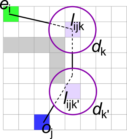
Figure 1: A shortest path going from entrance $e_{i}$ to objective $o_{j}$. Areas monitored by detectors $d_{k}$ and $d_{k}^{\prime}$ are those enclosed by circumferences. The segments of this path detected by each detector are shown with a dotted line and denoted by $l_{ijk}$ and $l_{ijk^{\prime}}$ respectively.

As mentioned before, the defense strategy is to place some detectors $d_{1},\dots,d_{\delta}$ on the map. Each of these detectors is characterized by a detection radius $\tau$, meaning that any attacker path intersecting the circle of radius $\tau$ centered at the detector is prone to fire an alarm that would elicit a neutralization response. Both events, alarm firing and neutralization are not deterministic in order to capture detector reliability and neutralization effectiveness respectively. More precisely, the alarm is fired with a probability that will be larger the longer the section of the path included in this detection circle, and the subsequent neutralization attempt will be successful with some probability $\theta$. This can be formalized as follows (see Table 1 for an overview of the notation used): let $P_{ij}$ be the shortest path between the $i$-th (out of $\varepsilon$) entrance $e_{i}$ and the $j$-th (out of $\phi$) objective $o_{j}$; if the attacker was too close to the objective within this path, no neutralization would be possible (he would reach the target before the enforcing agents could get to him), so let $\bar{P}_{ij}$ be the portion of the path $P_{ij}$ in which neutralization is still possible (assuming the attacker moves at speed $v$ and that $t_{n}$ seconds are required to neutralize him (Kaplan and Kress, 2005), this amounts to detracting a segment of length $vt_{n}$ from the end of $P_{ij}$). For each detector $d_{k}$, let $l_{ijk}$ be the portion of $\bar{P}_{ij}$ subject to detection by $d_{k}$ (see Figure 1 for an illustration), an event that will take place with probability

$$p_{ijk}=1-\exp(-\eta l_{ijk})$$ (1)

where $\eta>0$ is the detector’s instantaneous detection rate. Following (Nie et al, 2007), detectors work independently of one another, and therefore the total probability of non-detection $\tilde{D}_{ij}$ for path $P_{ij}$ is

$$\tilde{D}_{ij}=\prod_{k=1}^{\delta}(1-p_{ijk})=\prod_{k=1}^{\delta}\exp(-\eta l_{ijk})=\exp(-\eta\sum_{k=1}^{\delta}l_{ijk})$$ (2)

In this case (non-detection) or in case the attacker is detected but not effectively neutralized (something that will happen with probability $1-\theta$), the attacker will reach the objective $o_{j}$ causing a number of casualties $C_{j}$. Thus, the expected number of casualties $W_{ij}$ for this particular path will be

$$W_{ij}=\tilde{D}_{ij}C_{j}+(1-\tilde{D}_{ij})(1-\theta)C_{j}=C_{j}\left[\tilde{D}_{ij}\theta+(1-\theta)\right]$$ (3)

The total expected number of casualties will take into account all possible paths $P_{ij}$ the attacker can take, that is, between any entrance $e_{i}$ and objective $o_{j}$. To estimate this, let $\gamma_{ij}$ be the probability the attacker chose a particular path $P_{ij}$. Then,

$$W=\sum_{i=1}^{\varepsilon}\sum_{j=1}^{\phi}\gamma_{ij}W_{ij}$$ (4)

Next section will consider different scenarios depending on the particular modelization of values $\gamma_{ij}$, which capture the strategy used by the attacker to select a particular course of action.

2.2 Tackling Decision Making

The choice of values $\gamma_{ij}$ can be used to prioritize some targets and paths above others, and hence embodies the decision-making process done by the attacker. In previous works, i.e., (Nie et al, 2007; Yan and Nie, 2016; Cotta and Gallardo, 2017), a very simple approach was considered, namely that the attacker would pick with constant uniform probability any of these paths, that is,

$$\gamma_{ij}=\frac{1}{\varepsilon\phi}.$$ (5)

This can be regarded as a completely blind strategy in which the attacker is fully oblivious to both the damage that can be inflicted by targeting a particular objective or by the potential countermeasures taken by the defenders, and hence can be arguably considered as unrealistic. To tackle this issue, let us consider more informed strategies that take the previous points into account.

Let us firstly focus on the importance of each of the objectives. From the point of view of the attacker this is captured by values $C_{j}$ that indicate the population at objective $o_{j}$ (but that in a more general context could be also used to model any other feature of objectives whereby their targeting would be valuable for the attacker). An objective-aware strategy would thus preferably pick objectives of higher value over those with lower value. This can be done in a variety of ways, both from a qualitative point of view (considering the actual values $C_{j}$ or only their relative importance as in, e.g., their position in a ranked list) and from a quantitative point of view (given a certain prioritization index, how these are mapped to actual probabilities, thus determining how much preference is given to any objective). As a first step, in this work we have considered a strategy based on using the actual values $C_{j}$ and defining a proportional selection scheme based on these, i.e.,

$$\gamma_{ij}=\frac{C_{j}}{\varepsilon\sum_{k=1}^{\phi}C_{k}}$$ (6)

Thus, any objective $o_{j}$ will be targeted with a probability $p_{j}=\sum_{i=1}^{\varepsilon}\gamma_{ij}=C_{j}/C$, where $C=\sum_{k=1}^{\phi}C_{k}$ is the combined value of all objectives, i.e., $p_{j}\propto C_{j}$, being all paths to this objective equiprobable (again, more sophisticated strategies could be thought of here, but we initially assume this for simplicity).

Going one step beyond, let us consider awareness by the attacker of the presence of detectors. A game-theory perspective would be possible here, by considering that the attacker would select values $\gamma_{ij}$ to maximize his benefit (the inflicted damage) given whatever knowledge he has about the position of the detectors (or more generally about the strategy used by the defender to place these), and the defender would in turn place the detectors to minimize his loss given the knowledge he has about the attacker strategy. If we define $W[\Gamma,\Delta]$ to be the total number of casualties implied by a particular collection $\Gamma$ of values $\gamma_{ij}$ and a particular placement $\Delta$ of the detectors (i.e., a version of Equation 4 parameterized by $\Gamma$ and $\Delta$), we can see that the solution $(\Gamma^{*},\Delta^{*})$ given by

$$\Gamma^{*} = \underset{\Gamma}{\operatorname*{arg\,max}}{\left(W[\Gamma,\Delta^{*}]\right)}$$ (7)

$$\Delta^{*} = \underset{\Delta}{\operatorname*{arg\,min}}{\left(W[\Gamma^{*},\Delta]\right)}$$ (8)

defines a Nash equilibrium state: given a certain location $\Delta^{*}$ of the detectors, any different choice of values $\gamma_{ij}$ would result is less damage (i.e., a loss for the attacker), and conversely given the attacker’s strategy any other placement of the detectors would result in larger damage (i.e., a loss for the defender). Notice however that we are adopting here the position of the defender, and in principle it is not realistic to assume perfect knowledge of the attacker (although we can assume as a worst case scenario that the attacker has indeed this knowledge about the defender). Thus, if we place detectors at positions given by $\Delta$, we can assume that the attacker would pick $\Gamma$ to inflict the highest damage as indicated by Equation 7. It then follows that we should pick

$$\Delta^{\circ}=\underset{\Delta}{\operatorname*{arg\,min}}{\left(\underset{\Gamma}{\max}(W[\Gamma,\Delta])\right)}$$ (9)

In order to compute the term inside the outer parentheses in the previous equation we could exploit the fact that $W[\Gamma,\Delta]$ is linear in values $\gamma_{ij}$ and solve a linear program given by

$$\max W[\Gamma,\Delta]=\max\sum_{i=1}^{\varepsilon}\sum_{j=1}^{\phi}\gamma_{ij}W[\Delta]_{ij}$$ (10)

subject to

$$\sum_{i=1}^{\varepsilon}\sum_{j=1}^{\phi}\gamma_{ij} = 1$$ (11)

$$0\leqslant\gamma_{ij} \leqslant 1\qquad\forall i\in\{1,\dots,\varepsilon\},j\in\{1,\dots,\phi\}$$ (12)

where $W[\Delta]_{ij}$ is the value given by Equation 3 parameterized by $\Delta$. We do not need to use a linear programming solver though, since the solution to Equation 10 can be shown to be

$$\gamma_{ij}=\begin{cases}1&W[\Delta]_{ij}=\underset{i^{\prime}j^{\prime}}{\max}{(W[\Delta]_{i^{\prime}j^{\prime}})}\\ 0&{\rm otherwise}\end{cases}$$ (13)

i.e., the probability would be concentrated on the path that leads to the largest expected number of casualties (which we shall term the critical path) given the current distribution $\Delta$ of detectors. This follows easily from the fact that $W[\Gamma,\Delta]$ is a convex combination of values $W[\Delta]_{ij}$. Let $i^{\circ},j^{\circ}$ be the indices corresponding to the critical path (i.e, $\gamma_{i^{\circ}j^{\circ}}=1,\gamma_{ij}=0$ otherwise). The resulting value of Equation 10 for this solution would be $W[\Delta]_{i^{\circ}j^{\circ}}$, which by virtue of Equation 13 is no smaller than any other $W[\Delta]_{ij}$, $i,j\neq i^{\circ},j^{\circ}$. Thus, for any other alternative solution with $\gamma_{i^{\circ}j^{\circ}}=1-\alpha$, $0<\alpha\leqslant 1$, we would have the objective function decreased by $\alpha W[\Delta]_{i^{\circ}j^{\circ}}$ and increased at most by $\alpha W[\Delta]_{i^{\prime}j^{\prime}}$ where $W[\Delta]_{i^{\prime}j^{\prime}}$ is the second largest expected number of casualties, and hence the resulting value of the objective function would be reduced.

Computing the global minimum as per Equation 9 is not trivial, and will be dealt with in next section via heuristic approaches. Let us anyway assume that we have found this $\Delta^{\circ}$, and let $\Gamma[\Delta^{\circ}]$ be the corresponding path probabilities following Equation 13. We can see that in purity the state given by $(\Gamma[\Delta^{\circ}],\Delta^{\circ})$ is not a Nash equilibrium point: if $\Delta^{\circ}$ is fixed it is certainly the case that the attacker would not benefit from picking different path probabilities as shown before; however, taking these path probabilities as fixed, the defender could in general reduce the damage by relocating the detectors so as to have better coverage of the critical path. This may result in this path no longer being the critical path, hence implying the attacker would pick a different $\Gamma$; therefore, in general there may not be a Nash equilibrium. At any rate, this point $(\Gamma[\Delta^{\circ}],\Delta^{\circ})$ does indeed capture some kind of equilibrium, were we to assume that the attacker knows the defender’s strategy, namely that the worst-case casualties are to be minimized without taking any risks and vice versa, i.e., the defender knows the attacker will act accordingly to maximize his goals, each one being also aware of their own strategy being known by the opponent.

3 Materials and Methods

In light of the problem setting defined in the previous section, we need to solve the problem from the perspective of the defender by defining the location of each of the detectors. This will be done by using different (meta)heuristic approaches as shown below. In all cases, the objective will be minimizing Equation 4, namely the expected number of casualties $W[\Gamma,\Delta]$. As shown before, this quantity depends on the location of the detectors $\Delta$ (which is the actual degree of freedom of the formula, that is, the part of the equation that will be decided by the optimization algorithm) and the path probabilities $\Gamma$ (which will be given by any of the two scenarios depicted before, that is, fixed and known in advance to be proportional to the importance of each objective, or variable and known to correspond to the critical path implied by the current location of detectors). Next we will provide more details about the algorithms considered for this optimization endeavor, as well as about the benchmark we have used to test these.

3.1 Algorithmic Approaches

In this section we describe different algorithmic approaches that we have considered in order to tackle the problem, namely a Greedy Algorithm, a Local Search Procedure, a Tabu Search Metaheuristic and an Evolutionary Algorithm.

In all cases, the computational cost needed to evaluate a solution can be significantly reduced if some preprocessing is done over the problem instance being considered before starting the optimization process itself. This preprocessing is the same for all the algorithms and thus affects in the same way their performances. More precisely, a cache memory has been precomputed corresponding to the length of the segment of a path that would be detected in case a detector were placed at a specific cell in the map. These intersecting lengths are independently stored for each possible path going from one of the entrances in the map to one of the objectives. Besides, a dominance memory ${\Delta}=\{\Delta_{ij}\}_{m\times n}$ is also used to prune to some extent the search space that should be explored in order to optimize an specific instance. The implementations of both of these memories are more precisely described in (Cotta and Gallardo, 2017) and we refer the reader to that work for full details.

3.2 Greedy Algorithm

The algorithm described in this section (denoted as Greedy) corresponds to the one originally proposed by Nie et al (2007). This algorithm is a constructive method hence it places on the map the $\delta$ detectors one after the other. The extension of the current partial solution is done by adding on each step the detector which leads to a better local extension.

Input: $\delta$ (number of detectors to be placed)

1 $\mathit{candidates}:=\{(r,c)\ |\ 1\leqslant r\leqslant m,1\leqslant c\leqslant n,A_{rc}$ is unblocked $,\Delta_{r,c}<\delta\}$;

2 $\mathit{sol}:=\varnothing$;

3 while $\mathit{length}(\mathit{sol})<\delta$ do

4       $\mathit{fitness}^{*}:=\infty$;

5       $\mathit{detector}^{*}:=\mathrm{null}$;

6       for $d\in\mathit{candidates}$ do

7             $\mathit{tentative}:=\mathit{sol}+\{d\}$;

8             if $\mathit{value}(\mathit{tentative})<\mathit{fitness}^{*}$ then

9                   $\mathit{detector}^{*}:=d$;

10                   $\mathit{fitness}^{*}:=\mathit{value}(\mathit{tentative})$;

11                  

12             end if

13            

14       end for

15      $\mathit{sol}:=\mathit{sol}+\{\mathit{detector}^{*}\}$;

16       $\mathit{candidates}:=\mathit{candidates}\setminus\{\mathit{detector}^{*}\}$;

17      

18 end while

19return $\mathit{sol}$;

Algorithm 1 Greedy Algorithm

The corresponding pseudo-code is shown in Algorithm 1. Firstly, all non-blocked cells in the map minus those that are dominated by at least $\delta$ cells are taken as potential detector placements (line 1). Then, starting from an empty solution (line 2), the $\delta$ detectors are added to the current partial solution ($\mathit{sol}$) one at a time (lines 3-15). On each iteration, the candidate detector whose incorporation leads to the best extended solution –i.e., the one locally minimizing the total number of casualties given the current location of detectors and the attacker model considered– is selected (lines 6-12), added to the solution (line 13) and removed from the set of candidate detectors (line 14).

As a greedy algorithm, this procedure makes different locally optimal decisions and hence the resulting final solution cannot be guaranteed to result optimal.

3.3 Hill Climbing

We also consider a Hill Climbing (HC) Local Search algorithm. In contrast to constructive methods –such as the Greedy method described above– which work with a partial solution, these algorithms work with a complete solution during the optimization process (Aarts and Lenstra, 1997; Hoos and Stützle, 2005). A crucial concept here is that of neighborhood which refers to the set of solutions which can be obtained from current one by modifying one part of the solution. The algorithm starts from a complete solution that should be constructed somehow. Subsequently, solutions in the neighborhood of the current one are examined and evaluated and a move towards one of these is performed in case the quality of such solution improves the current one. This process will be repeated until no solution in the neighborhood of the current one provides any improvement. At this point, a local optimum to the problem has been found and is returned. The whole process can be iterated starting from different initial solutions until the allowed execution time is exhausted, returning the best found solution at the end.

The pseudo-code for this procedure is shown in Algorithm 2. $sol$ stands for a complete solution, implemented as a vector of different locations for placing the detectors. The algorithm explores the neighborhood of the current solution by substituting one detector location in the current solution by each of the unused candidate locations for the problem instance ($\textsc{Replace}(\mathit{sol},i,d)$ denotes the solution that is obtained by replacing the $i$-th detector in solution $\mathit{sol}$ by the alternative detector $d$ – see line 7). Then the best modified solution is selected (lines 8-11). If this selected solution is better than the current one, a move is done towards the new solution (line 9) and an improvement has been achieved (line 10). Starting from this improved solution, the same procedure is done for the remaining detectors, and this process is repeated until a local optimum is reached, i.e., when no further improvement is possible.

Input: $\mathit{sol}$ (a collection with the coordinates of $\delta$ detectors)

1 $\mathit{candidates}:=\{(r,c)\ |\ 1\leqslant r\leqslant m,1\leqslant c\leqslant n,A_{rc}$ is unblocked$,\Delta_{rc}<\delta\}$;

2 $\mathit{improvement}:=\mathrm{true}$;

3 while $\mathrm{improvement}$ do

4       $\mathit{improvement}:=\mathrm{false}$;

5       for $i:=1$ to $\mathit{length}(\mathit{sol})$ do

6             for $d\in(\mathit{candidates}\setminus\{d\,|\,d\in\mathit{sol}\})$ do

7                   $\mathit{tentative}:=\textsc{Replace}(\mathit{sol},i,d)$;

8                   if $\mathit{value}(\mathit{tentative})<\mathit{value}(\mathit{sol})$ then

9                         $\mathit{sol}:=\mathit{tentative}$;

10                         $\mathit{improvement}:=\mathrm{true}$;

11                        

12                   end if

13                  

14             end for

15            

16       end for

17      

18 end while

19return $\mathit{sol}$;

Algorithm 2 Hill Climbing Algorithm

3.4 Tabu Search

Tabu Search (TS) is a metaheuristic originally proposed by Glover (1989, 1990) that has been successfully used for the resolution of different combinatorial optimization problems. The key idea in TS is to use a memory data structure in order to keep track of the previous history of the search. This memory is referred to as the Tabu List, as moves towards solutions included in this list are forbidden. This memory serves the purpose of avoiding revisiting recently explored solutions, thus allowing the algorithm to avoid to a certain extent the possibility of getting trapped in cycles during the search process. At each iteration, the search moves towards the best solution in the neighborhood of allowed moves. Since all improving solutions may be forbidden, moves towards solutions worse than the current one may be performed and this is the mechanism allowing the algorithm to escape from local optima. As keeping all visited solutions in a list is not memory efficient, an usual alternative consists of using a data structure keeping track of attributes of recently visited solutions, and forbidding moves towards solutions with those same attributes for some iterations (the so called tabu tenure).

Our implementation of a TS algorithm is shown in Algorithm 3. A solution corresponds to a vector with $\delta$ locations. The neighborhood of a solution consists of all solutions that can be obtained from that one by moving one of its detectors to another location not included in the solution. As tabu structure, we use a matrix ${T}=\{T_{ij}\}_{m\times n}$ so that $T_{ij}$ records tabu information for doing a move consisting in placing a detector at cell $i\times j$ in the map. $\mathit{sol}$ is the solution currently being explored and $\mathit{best}$ is the best solution found so far. The algorithm repeats the following process, with a limit on the number of iterations to perform in case no improved solution is attained:

• All moves leading to solutions in the neighborhood of the current one which are not currently tabu are considered and those producing solutions with the best value are collected into $\mathit{bestMoves}$ set (lines 5-18). Additionally, if one solution in the neighborhood is better than the best one found so far (the so named aspiration criteria), this solution is also considered even if the corresponding move were forbidden by the tabu memory.

• Then, one specific move among the best ones is randomly chosen (line 19) and performed (line 20). Recall that a move displaces one detector to a new position. Trying to move one detector to this same position is set as tabu for a number of iterations (line 21).

• Finally, if the new solution is the best one found so far, it is recorded and an improvement is acknowledged (lines 23-24). Otherwise, we record that this iteration was unable to achieve any improvement (line 26).

Just like in the case of Hill Climbing algorithm, the whole process is repeated several times until the allowed execution time is exhausted, and the best solution found is returned at the end.

Input: $\mathit{sol}$ (a collection with the coordinates of $\delta$ detectors)

1 $\mathit{candidates}:=\{(r,c)\ |\ 1\leqslant r\leqslant m,1\leqslant c\leqslant n,A_{rc}$ is unblocked$,\Delta_{rc}<\delta\}$;

2 $\mathit{best}:=\mathit{sol}$;

3 $\mathit{noImprovement}:=0$;

4 while $\mathit{noImprovement}<\mathit{maxIters}$ do

5       $\mathit{bestMoves}:=\varnothing$;

6       $\mathit{bestMovesValue}:=\infty$;

7       for $i:=1$ to $\mathit{length}(\mathit{sol})$ do

8             for $(r,c)\in(\mathit{candidates}\setminus\{d\,|\,d\in\mathit{sol}\})$ do

9                   $\mathit{tentative}:=\textsc{Replace}(\mathit{sol},i,(r,c))$;

10                   if $\textbf{not}\ \textsc{Tabu}(T,r,c)\ \textbf{or}\ \mathit{value}(\mathit{tentative})<\mathit{value}(\mathit{best})$ then

11                         if $\mathit{value}(\mathit{tentative})=\mathit{bestMovesValue}$ then

12                               $\mathit{bestMoves}:=\mathit{bestMoves}+\{\mathit{(i,r,c)}\}$;

13                              

14                         else if $\mathit{value}(\mathit{tentative})<\mathit{bestMovesValue}$ then

15                               $\mathit{bestMoves}:=\{\mathit{(i,r,c)}\}$;

16                               $\mathit{bestMovesValue}:=\mathit{value}(\mathit{tentative})$;

17                              

18                        

19                   end if

20                  

21             end for

22            

23       end for

24      $\mathit{(i,r,c)}:=\textsc{chooseFrom}(\mathit{bestMoves})$;

25       $\mathit{sol}:=\textsc{Replace}(\mathit{sol},i,(r,c))$;

26       $\textsc{setTabu}(T,r,c)$;

27       if $\mathit{value}(\mathit{sol})<\mathit{value}(\mathit{best})$ then

28             $\mathit{best}:=\mathit{sol}$;

29             $\mathit{noImprovement}:=0$

30       else

31             $\mathit{noImprovement}:=\mathit{noImprovement}+1$

32       end if

33      

34 end while

35return $\mathit{best}$;

Algorithm 3 Tabu Search Algorithm

3.5 Evolutionary Algorithm

An Evolutionary Algorithm (EA) (Eiben and Smith, 2003) is a optimization procedure inspired by the biological evolution of species. These algorithms are population based ones which means that a pool of solutions is maintained during the optimization process. This population of solutions is initialized somehow before entering the evolutionary loop in which solutions go through different processes such as reproduction, recombination, mutation and replacement. At the end of the evolutionary loop, the best solution found during the execution of the algorithm is returned.

Algorithm 4 shows the specific incarnation of the EA that we have used. $\mathit{pop}$ is the population of non-repeated $\mathit{popSize}$ individuals, each one being a full solution to the problem. Like in previous heuristics, the search space explored by the EA is restricted to non-blocked cells in the map minus those that are dominated by at least $\delta$ cells. Each individual in the population of solutions is initialized randomly as a vector of $\delta$ different locations for placing each detector. These locations are randomly chosen in an uniform way among all possible ones (lines 1-4). Then, the following process corresponding to the evolutionary loop is repeated, until the maximum allowed execution time for the algorithm is exhausted:

• With probability of selection $p_{X}$, two individuals acting as parents are selected from the population (lines 7-9). The specific algorithm used for each selection is binary tournament selection in which, after picking two individuals at random, the best one is selected. Now, these individuals go through recombination in order to produce a new one. For this purpose, let us consider the set comprising the union of detector placements included in to be recombined individuals. A new individual, constituting the offspring for this generation, is then defined by sampling in a uniform way $\delta$ elements (i.e., detector placements) from this previous set.

• Otherwise (i.e. with probability $1-p_{X}$) recombination is not performed and a random individual of current population is selected as the offspring (line 11).

• Each detector location in the the offspring is mutated with probability $p_{m}$. More precisely, with such probability the corresponding detector is replaced with another one not included in the solution (line 13). The resulting individual is evaluated (line 14).

• As to replacement, the worst individual currently included in the population is replaced by the offspring (line 15).

Finally, when the execution time limit is reached, the best individual found along this whole process is returned as a solution.

Input : $\mathit{popSize}$ (population size)

$p_{X}$ (recombination probability)

$p_{m}$ (mutation probability)

1 for $i:=1$ to $\mathit{popSize}$ do

2       $\mathit{pop}_{i}:=$ RandomIndividual$()$;

3       Evaluate($\mathit{pop}_{i}$);

4      

5 end for

6while allowed runtime not exceeded do

7       if recombination is performed($p_{X}$) then

8             $parent_{1}:=$ Select($\mathit{pop}$);

9             $parent_{2}:=$ Select($\mathit{pop}$);

10             $\mathit{offspring}:=$ Recombine($parent_{1}$, $parent_{2}$);

11            

12      else

13             $\mathit{offspring}:=$ Select($\mathit{pop}$);

14            

15       end if

16      $\mathit{offspring}:=$ Mutate($p_{m},\mathit{offspring}$);

17       Evaluate($\mathit{offspring}$);

18       $\mathit{pop}:=$ Replace($\mathit{pop}$, $\mathit{offspring}$);

19      

20 end while

21return best solution found;

Algorithm 4 Evolutionary Algorithm

3.6 Problem Instances

In order to test the algorithms described in the previous section in a broad set of conditions, we have generated problem instances that try to resemble different real-world scenarios. To be precise, we have considered the following three classes of maps:

• harbour: these problem instances represent a coastal area that may be subject to a maritime attack by a small vessel, cf. (Yan and Nie, 2016). These maps feature a large inner open area (representing a water mass such as a lake or a sheltered body of sea) typically comprising several scattered islands, surrounded by a complex coastline with some straits from which the attacker can enter the threat area. See Figure 2a.

• newtown: these problem instances represent a modern urban area in which streets run in straight lines creating a grid (Manhattan or Barcelona’s Expansion District being prominent examples). These maps feature streets of different width running at right angles, as well as a number of plazas of different sizes scattered across the map. See Figure 2b.

• oldtown: these problem instances represent the historic core of an old town. As such, the street plan features a much more decentralized and flexible structure. Streets typically originate at plazas and run in different directions and angles with respect to each other, bifurcating as they get farther from the plazas. See Figure 2c.

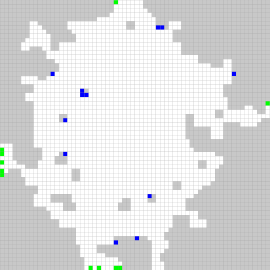
(a)

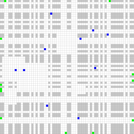
(b)

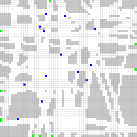
(c)

Figure 2: Examples of each of the three scenarios considered. (a) harbour (b) newtown (c) oldtown.

For each of these three problem classes, we have defined a map generator in order to create a number of instances of the desired characteristics, hence contributing to the diversity of the benchmark. Next we will describe in more detail the generation procedure for each map class.

3.6.1 Coastal Area

These maps are created in two phases. In the first phase a exponentially decaying diffusion mechanism is used to grow the inner water mass: we start at the center of the lattice with a value $p=1$; with this probability we set the current position to unblocked and move to each of the four neighbors in a von Neumann topology (i.e., North, East, South, West), having this probability decay by a different factor $\{\beta_{i}\}_{1\leqslant i\leqslant 4}$, that depends on the direction, and repeating the process from each of them. When the diffusion stops, we proceed with the second phase in which the map is smoothed out by using a cellular automaton which has each lattice cell change to the most repeated state among itself and its neighbors. This process is run until convergence or after a maximum number of iterations has been performed.

Once the above is done, objectives are placed on positions along the coastline. To do so, a random unblocked position is selected, and a random walk (using the von Neumann connectivity mentioned before) is performed until a blocked position is found. This position is then unblocked and defined as an objective. The process is repeated as many times as objectives need to be placed. The entrances are randomly selected among the unblocked positions on the borders of the map.

3.6.2 Modern Urban Area

These maps are also created in two phases: in the first one the street grid is created, and in the second one a number of plazas are added to the map. In order to tackle the first part, we consider values $\{p_{i}\}_{0\leqslant i}$, representing the probability of having a street of width $i$ (the value $p_{0}$ corresponding to the situation of not having a street at all). Using these, we traverse the columns of the maps deciding whether we include a North-South street and if so of which width. In case a street of width $w$ is placed, we jump $w+1$ columns to the right and repeat the procedure until all columns have been processed. The whole process is then repeated by traversing rows of the maps in order to place West-East streets.

The second phase involves placing some plazas on the map. This is controlled by parameter $n_{p}$ indicating the number of plazas and values $\{q_{i}\}_{\min_{p}\leqslant i}$ representing the probability of having a square plaza of a certain side length, where $\min_{p}$ indicates the minimum side length admissible. The generator would iterate $n_{p}$ times a process of determining the size of a plaza using probabilities $\{q_{i}\}$ and then deciding a suitable location given this size. As in the previous scenario, the entrances are randomly selected among the unblocked positions on the borders of the map. As to the objectives, these are placed in random unblocked positions of the map.

3.6.3 Old Historic Town

These maps are created by iterating $n_{p}$ (a parameter that just like in the previous scenario indicates a number of plazas to be located on the map) times a basic procedure. This procedure consists of determining the size of a plaza (using a collection of values $\{q_{i}\}_{\min_{p}\leqslant i}$ as in the newtown scenario), placing it in on the map, and then having four streets depart from each of the sides of the plaza. These streets do not run at right angles though: they are laid out having a certain slope between $\pm 1$ (a diagonal street) and $\pm\max_{s}$ (closer to horizontal or vertical). The width of the street is set to $w$ and as the street runs out from the plaza it can branch along the way into a smaller (width $w-1$) street with probability $p_{b}$. These branched-out streets can in turn branch into smaller lanes in a recursive way, thus trying to resemble the complex and more convoluted network of small streets and lanes in the historic core of old towns.

Much like it was done in harbour and newtown, the entrances are randomly selected among the unblocked positions on the borders of the map. As to the objectives, these are placed in random unblocked positions of the map as in newtown.

4 Experimental Results

In order to evaluate the performance of the algorithms we have followed a problem generator approach (De Jong et al, 1997), whereby rather than running each algorithm multiple times on the same problem instance, they are run once on a different problem instance each time, thus allowing to obtain a more representative measure of performance across the whole set of possible instances, and avoiding (or at the very least diminishing the impact of) any spurious match between a specific instance and a specific algorithm. More precisely, all algorithms have been run twenty five times on each of the three problem classes, namely harbour, newtown and oldtown, for the two attacker scenarios (i.e., proportional selection of objectives and worst-case equilibrium) using the same seventy five problem instances in all cases.

The maps considered have been generated on a grid of size $64\times 64$. In all cases, the number of entrances $\varepsilon$ and the number of objectives $\phi$ are independently chosen uniformly at random between 10 and 15. A 10% region around the borders of the maps is kept free of objectives to avoid any of these being located extremely close to an entrance, something which could be regarded as a pathological case. As to scenario dependent parameters, in the case of harbour, the decay parameters $\{\beta_{i}\}$ were randomly picked between 0.98 and 0.99 and checked to empirically ensure that the diffusion barely reached the borders of the map. The dimension of each cell in the map was of 200m $\times$ 200m and the detection radius for the detectors was set to $\tau=500m$. Regarding newtown, each map has a random number of plazas $n_{p}$ between 3 and 6, whose side length can range between 4 and 13 ($\{q_{i}\}_{4\dots 13}=1/10$). Street widths are selected using values $\{p_{i}\}_{0\dots 3}=\{0.5,0.25,0.15,0.1\}$. Finally, oldtown maps also comprise a random number of plazas $n_{p}$ between 3 and 6, whose sizes range from 6 up to 15 ($\{q_{i}\}_{6\dots 15}=1/10$). The maximum slope of streets is 1/5 of the map side length, they have initial width $w=3$, and can branch with probability $p_{b}=0.02$. For these instances representing different town configurations, the dimension of each cell in the map was of 5m $\times$ 5m and the detection radius for the detectors was set to $\tau=20m$.

We have considered that minimum time required to neutralize an attacker is $t_{n}=10$s. In the case of newtown and oldtown instances, this means that effective neutralization is not possible if the distance of the attacker to the objective is less than 10m, which corresponds to assuming that the attacker moves at a speed $v=1$m/s. In the case of harbour instances, we have assumed a moving speed for the vessels $v=20$m/s and thus the maximum distance to the objective for being able to abort the attack is 200m. As to the detector’s instantaneous detection rates, we have used a value of $\eta=0.06$ for the newtown and oldtown instances and $\eta=0.006$ for the harbour instances, thus assuming that detectors are less reliable in the later case. For the probability of effectively neutralizing a detected attacker, we used $\theta=0.6$ in all cases. Additionally, in order to estimate the expected number of casualties for an objective cell $\{C_{j}\}_{1\dots\phi}$, we used the same procedure defined by Cotta and Gallardo (2017) which is in turn based on Equation 2 in (Kaplan and Kress, 2005). This equation presumes that the number of fragments produced after the explosion tends to $\infty$ and that these fragments and individuals around the target area are spatially distributed according to a Poisson process. We have used the same parameters for this equation as those proposed by Nie et al (2007), except for the population densities near each objective cell, which were set as a constant therein but which we have modelled as a random variable instead, with the aim of considering more diverse instances. For newtown  and oldtown instances this is chosen from a normal distribution ${\mathcal{N}(0.4,0.1)}$ persons / ${\mathrm{m}}^{2}$, whereas in the case of harbour instances, we take ${\mathcal{N}(9\cdot 10^{7},1.8\cdot 10^{6})}$ (these latter values do not really stand for an expected number of civilian casualties but instead represent the economical cost resulting from damaging the corresponding objective). Overall, all parameters have been picked to have generated instances resemble realistic scenarios, as described in the literature (Kaplan and Kress, 2005; Nie et al, 2007; Yan and Nie, 2016), while providing diversity thanks to their range of variability.

Regarding the parameters used for the different algorithms, the following settings were used for the EA: population size $\mathit{popSize}=100$ individuals, probability of crossover $p_{X}=0.9$ and probability of mutation $p_{m}=1/\delta$. The tenure value for the TS algorithm was a random number of iterations in $[\delta\dots 2\delta]$. All algorithms were run for 30 seconds on each instance (the hardware platform used was a cluster of Intel Xeon E7-4870 2.4 GHz processors with 2GB of RAM running under SUSE Linux Enterprise Server 11 operating system).

Figure 3: Deviation (%) from the best known solution for each algorithm and data set as a function of the number of detectors used in the proportional selection scenario. Notice the different scale on the Y axis in each subfigure.

Figure 4: Deviation (%) from the best known solution for each algorithm and data set as a function of the number of detectors used in the worst-case equilibrium scenario. Notice the different scale on the Y axis in each subfigure.

The results are depicted in Figures 3–4. In the two scenarios, the three iterative approaches largely outperform the greedy algorithm. In most cases, the latter seems to experience a peak of difficulty when the number of detectors is about the same magnitude as the number of objectives. This can be explained by the fact that for a low number of detectors the number of options are limited and the greedy selection is often reasonably close to more finely adjusted solutions, whereas for a large number of detectors these can be spread to cover most paths without not so much difficulty (thus leaving the middle regime between these two extremes as the most complex one).

This said, it is much more interesting to note the difference between the two scenarios. Notice firstly how the range of deviations for all algorithms is larger in the worst-case equilibrium scenario. It is not difficult to see that this latter scenario is indeed harder from an optimization point of view, due to the complex structure of the search landscape in this case: the quality of a solution is dictated by the critical path given the current location of detectors; hence, the optimization algorithm will attempt to gradually increase the coverage of this critical path but in doing so (i) it will have to take care of not leaving uncovered other paths to objectives of higher sensitivity, and (ii) eventually the critical path may turn to be a different one (recall the discussion in Section 2.2) causing an abrupt discontinuity in the direction of the optimization process. This differs from the proportional selection scenario, in which the objective function is a weighted combination whose coefficients are fixed, and hence can be optimized in a more smoothly way. Furthermore, notice how the search landscape is prone to have mesas in the worst-case equilibrium scenario, given the fact that as long as the coverage of the critical path does not change and the coverage of other paths does not change enough for the critical path to be a different one, the value of the objective function will be the same. This may affect all algorithms, and in particular the greedy algorithm (see the insets in Figure 5), which will face the need to pick a choice among a large number of seemingly equivalent options.

(a)

(b)

Figure 5: Cumulative boxplot of deviations (%) from the best know solution for each algorithm. The main plot focus on the iterative heuristics, and the inset includes the greedy algorithm as well. (a) Proportional selection (b) Worst-case equilibrium. Notice the different scale on the Y axis in each subfigure.

Table 2: Results of Holm Test in the proportional selection scenario using Hill Climbing as control algorithm.

$i$		algorithm	$z$-statistic	$p$-value	adjusted $p$-value
1		EA	3.38e$+$00	3.66e$-$04	3.66e$-$04
2		TS	4.56e$+$00	2.51e$-$06	5.01e$-$06
3		Greedy	9.22e$+$00	1.49e$-$20	4.46e$-$20

Table 3: Results of Holm Test in the worst-case equilibrium scenario using the Evolutionary Algorithm as control algorithm.

$i$		algorithm	$z$-statistic	$p$-value	adjusted $p$-value
1		HC	1.64e$+$00	5.02e$-$02	5.02e$-$02
2		TS	3.29e$+$00	5.08e$-$04	1.02e$-$03
3		Greedy	8.22e$+$00	1.05e$-$16	3.16e$-$16

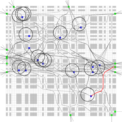
(a)

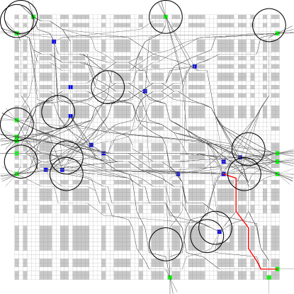
(b)

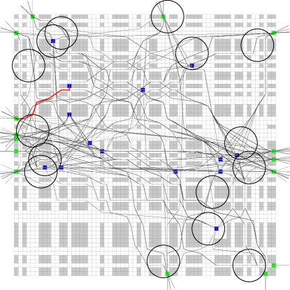
(c)

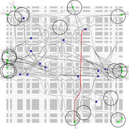
(d)

Figure 6: Illustrative solutions found by each of the algorithms on a newtown instance with 15 detectors. (a) Greedy (b) HC (c) TS (d) EA. Notice the critical path (shown in red) is different in each case.

As a result of the previous considerations, there is a difference between the relative behavior of the different iterative algorithms in each of the two scenarios. In the first one (proportional selection), HC is significantly better than the other algorithms (Quade test $p$-value $\approx 0$, Holm test results shown in Table 2). However, in the worst-case equilibrium scenario the EA provides better results (Quade test $p$-value $\approx 0$, Holm test results shown in Table 3). Indeed, if we perform a head-to-head comparison between HC and EA in this latter scenario by means of a signrank test, we observe that the EA is significantly better with $p$-value = 0.0057. Quite interestingly, if we break down the analysis by map class, we find that HC is negligibly and non-significantly better than EA in the harbour class ($p$-value = 0.7422), and that the EA is significantly better than HC in newtown and oldtown ($p$-values of 0.0098 and 0.0020 respectively). As a matter of fact, the quantitative difference between the algorithms is clear if we observe the distribution of deviations from the best known solutions (Figure 5): the difference in favor of HC is much smaller in the proportional selection scenario when compared to the difference in favor of EA in the worst-case equilibrium scenario. Clearly, the more complex nature of the search landscape is better dealt with via the diversification of a population-based approach than the strong intensification of the HC algorithm considered.

Figure 6 shows an example of the solutions provided by either algorithm on a newtown map for the worst-case equilibrium scenario. The solutions provided by each algorithm are structurally different. The greedy approach tends to place the detectors in the vicinity of the objectives. The local search approaches seem to have found solutions in which detectors are usually placed close to entrances, but with some detectors being placed next to objectives as well. Finally the EA has also favored locations close to entrances in order to cover a large number of paths; however, it has also identified a few crossroads that seem to be important in order to maximize coverage of many paths. Notice how for each of these solutions, the resulting critical path is different in each case.

5 Conclusions and Future Work

Counterterrorism is a multidimensional endeavor that spreads along many entangled fronts. One of them is undoubtedly the tactical defense against targeted attacks, from which suicide bombings constitute a heinous distinguished example. While low-rank individuals engaged in international terrorism groups may be often fanaticized and hence can have motivations that challenge rational analysis (or motivations that, while rational, can be directed towards other personal or social goals than those of the terror group as a whole (Abrahms, 2008)), their actions are often dictated by or inspired by the guidelines emanating from the upper levels of a command hierarchy, more prone to engage in analytical considerations of cost-effectiveness in pursue of their criminal goals. As a matter of fact, the assessment of the situation would not qualitatively change if rather than considering a suicide attacker embarked on a no-return mission we consider the case of an unmanned attack using a drone or any other suitable vehicle (Patterson and Patterson, 2010), a scenario slanted towards purely tactical considerations. In any case, assuming this operational context provides at the very least a worst-case scenario upon which a better informed, more down-to-earth strategy could be built with the help of adequate intelligence. The availability of cogent tools to aid in the analysis of these scenarios can thus be most helpful. In this sense, we have considered in this work the use of different heuristic approaches to determine the most appropriate deployment of sensors so as to detect perpetrators of bombing attacks in a given threat area, aiming to minimize the number of casualties or economic damages. Modeling this situation as an adversarial game in which the attacker is cognizant of the location of these detectors and tries to target the most cost-effective objective turns out to pose a challenging optimization task. Among the algorithms considered and tested on a variety of problem scenarios, an evolutionary algorithm turns out to be quite effective. It is however remarkable that a simple hill climber performs reasonably well on some instances, suggesting that an eventual hybridization of both methods into a memetic approach (Neri et al, 2012) might be very promising.

Future work will be actually directed in the direction of hybridizing methods, aiming to exploit their synergy. Pushing the limits of the resulting techniques (in terms of, e.g., the size of the maps, the number of objectives, etc.) would be of paramount interest. Also, it is conceivable to consider in the context described in this work extensions of the underlying model including different types of detectors, cf. (Yan and Nie, 2016), or even introducing a dynamic component in the configuration of the ground map.

References

- Aarts and Lenstra (1997) Aarts EHL, Lenstra JK (1997) Local Search in Combinatorial Optimization. John Wiley & Sons
- Abrahms (2008) Abrahms M (2008) What terrorists really want: Terrorist motives and counterterrorism strategy. International Security 32(4):78–105
- Blomberg et al (2004) Blomberg SB, Hess GD, Weerapana A (2004) An economic model of terrorism. Conflict Management and Peace Science 21(1):17–28
- Central Intelligence Agency (2003) Central Intelligence Agency (2003) National strategy for combating terrorism. https://www.cia.gov/news-information/cia-the-war-on-terrorism/Counter˙Terrorism˙Strategy.pdf, [Accessed 31 January 2018]
- Chicago Project on Security and Terrorism (2016) (CPOST) Chicago Project on Security and Terrorism (CPOST) (2016) Suicide attack database (April 19, 2016 release). [Data File]. Retrieved from http://cpostdata.uchicago.edu/
- Cotta and Gallardo (2017) Cotta C, Gallardo JE (2017) Metaheuristic approaches to the placement of suicide bomber detectors. Journal of Heuristics DOI 10.1007/s10732-017-9335-z
- De Jong et al (1997) De Jong KA, Potter MA, Spears WM (1997) Using problem generators to explore the effects of epistasis. In: Bäck T (ed) Proceedings of the 7th International Conference on Genetic Algorithms, Morgan Kaufmann, pp 338–345
- Edwards et al (2016) Edwards D, McMenemy L, Stapley S, Patel H, Clasper J (2016) 40 years of terrorist bombings – a meta-analysis of the casualty and injury profile. Injury 47(3):646–652
- Eiben and Smith (2003) Eiben AE, Smith JE (2003) Introduction to Evolutionary Computing. SpringerVerlag
- Ganor (2011) Ganor B (2011) Trends in modern international terrorism. In: Weisburd D, Feucht T, Hakimi I, Mock L, Perry S (eds) To Protect and To Serve. Policing in an Age of Terrorism, Springer, New York, pp 11–42
- Gares et al (2016) Gares KL, Hufziger KT, Bykov SV, Asher SA (2016) Review of explosive detection methodologies and the emergence of standoff deep UV resonance raman. Journal of Raman Spectroscopy 47(1):124–141
- Glover (1989) Glover F (1989) Tabu search-part I. ORSA Journal of Computing 1:190–206
- Glover (1990) Glover F (1990) Tabu search-part II. ORSA Journal of Computing 2:4–32
- Hoffman (2003) Hoffman B (2003) The logic of suicide terrorism. The Atlantic. http://www.theatlantic.com/magazine/archive/2003/06/the-logic-of-suicide-terrorism/302739/, [Accessed 2 July 2016]
- Hoos and Stützle (2005) Hoos H, Stützle T (2005) Stochastic Local Search. Foundations and Applications. Morgan Kaufmann
- Kaplan and Kress (2005) Kaplan EH, Kress M (2005) Operational effectiveness of suicide-bomber-detector schemes: A best-case analysis. Proceedings of the National Academy of Sciences of the United States of America 102(29):10399–10404
- Kim et al (2016) Kim M, Batta R, He Q (2016) Optimal routing of infiltration operations. Journal of Transportation Security 9(1):87–104
- Lara-Cabrera et al (2017) Lara-Cabrera R, González-Pardo A, Benouaret K, Faci N, Benslimane D, Camacho D (2017) Measuring the radicalisation risk in social networks. IEEE Access 5:10892–10900
- Leistedt (2016) Leistedt SJ (2016) On the radicalization process. Journal of Forensic Sciences 61(6):1588–1591
- Neri et al (2012) Neri F, Cotta C, Moscato P (eds) (2012) Handbook of Memetic Algorithms, Studies in Computational Intelligence, vol 379. Springer-Verlag, Berlin Heidelberg
- Nie et al (2007) Nie X, Batta R, Drury CG, Lin L (2007) Optimal placement of suicide bomber detectors. Military Operations Research 12(2):65–78
- Patterson and Patterson (2010) Patterson MR, Patterson SJ (2010) Unmanned systems: An emerging threat to waterside security: Bad robots are coming. In: 2010 International WaterSide Security Conference, IEEE Press, pp 1–7
- Rand Corporation (2009) Rand Corporation (2009) RAND database of worldwide terrorism incidents. [Data File] http://smapp.rand.org/rwtid/search˙form.php
- Tutun et al (2017) Tutun S, Khasawneh MT, Zhuang J (2017) New framework that uses patterns and relations to understand terrorist behaviors. Expert Systems with Applications 78:358–375
- Yan and Nie (2016) Yan X, Nie X (2016) Optimal placement of multiple types of detectors under a small vessel attack threat to port security. Transportation Research Part E: Logistics and Transportation Review 93:71–94