Participation bias in the estimation of heritability and genetic correlation
Abstract
It is increasingly recognized that participation bias can pose problems for genetic studies. Recently, to overcome the challenge that genetic information of non-participants is unavailable, it is shown that by comparing the IBD (identity by descent) shared and not-shared segments among the participants, one can estimate the genetic component underlying participation. That, however, does not directly address how to adjust estimates of heritability and genetic correlation for phenotypes correlated with participation. Here, for phenotypes whose mean differences between population and sample are known, we demonstrate a way to do so by adopting a statistical framework that separates out the genetic and non-genetic correlations between participation and these phenotypes. Crucially, our method avoids making the assumption that the effect of the genetic component underlying participation is manifested entirely through these other phenotypes. Applying the method to 12 UK Biobank phenotypes, we found 8 have significant genetic correlations with participation, including body mass index, educational attainment, and smoking status. For most of these phenotypes, without adjustments, estimates of heritability and the absolute value of genetic correlation would have underestimation biases.
1 Main
The rapid development of biobank studies provides an unprecedented opportunity for understanding the genetics across many phenotypes 1. At the same time, significant effort has been devoted to issues that complicate data analyses. These include population stratification, cryptic relatedness, assortative mating, and measurement error 2; 3; 4; 5. More recently, particularly for investigations that go beyond the testing of associations between phenotypes and individual genetic variants, it is increasingly appreciated that participation bias (PB), the ascertained samples are not fully representative of the population, can lead to misleading results 6. While PB is a concern for all sampling surveys, it is particularly difficult to avoid for genetic studies given the requirement of informed consent and the collection of DNA material. For example, despite the large sample size of UK Biobank (UKBB), the participation rate of those who were invited is only about 7, allowing for the possibility of substantial bias in some aspects of the data.
For sample surveys in general, a common approach to adjusting for ascertainment bias is to construct a propensity score based on variables, e.g., sex and educational attainment, whose distributional differences between sample and target population are known, or can be well approximated 8. By assuming that the systematic component of participation probability is fully captured by this score, analyses can be adjusted by applying inverse propensity weighting (IPW) to the samples. For genetic studies, it has been shown that participation can be associated with many phenotypes, such as educational attainment, alcohol use, mental and physical health 9; 10; 11; 12; 13; 14; 15. The UKBB participants are reported to be less likely to be obese, to smoke, to drink alcohol daily, and to have fewer self-reported health conditions compared with the general UK population.13. A recent study applied IPW to the UKBB data by creating a propensity score based on 14 phenotypes including age, BMI, weight, education, etc. 15 This propensity score, however, does not include genotypes. Thus, for analyses that involve genotypes, this adjustment would be sufficient only under the assumption that the systematic genotypic differences between sample and population are fully captured by this propensity score, which is equivalent to saying that the effect of the genetic component underlying participation is manifested entirely through this score, which can be considered as a composite phenotype. Previous results16 and results presented below show that this assumption is unlikely to hold.
While the effectiveness of IPW or any other adjustment methods based only on phenotypes is doubtful, there is no obvious alternative unless genotype difference between sample and population can be independently estimated without relying on the phenotypes, which is difficult given that genotypes of non-participants are unavailable. A recent publication showed that the sample-population allelic frequency differences can be estimated by comparing the IBD (identity by descent) shared and not-shared segments among the participants. Here we utilize information obtained from that method through introducing a statistical model that specifies a genetic and a non-genetic component for each of the participation variable and the other phenotypes. The model separates out the genetic and non-genetic correlations between participation and other correlated phenotypes, and allows us to obtain adjusted estimates of heritability and genetic correlation for these phenotypes that take PB into account.
This model includes the IPW model as a special case. Theoretically, without adjustments, heritability and genetic correlation can be over-estimated or under-estimated depending on the relative magnitudes of the genetic and non-genetic correlations between participation and the phenotypes. Empirically, we applied the adjustment method to 12 phenotypes of the UKBB data, and found that, without adjustment, heritability and the absolute value of the genetic correlation estimates tend to be underestimated for most of them.
2 Results
2.1 Participation model overview
In practice, participation is often a two-step process. In the first step, a group of individuals are invited to participate in the study, and in the second step the invited make the decision whether to participate. For simplicity, we consider a model where the bias is only in the second step, the invited list is representative of the target population. Consequences of the violation of this assumption are discussed later. For the second step, as in Benonisdottir and Kong (2023)16, we adopt a liability-threshold model where the liability score of a person is denoted by , which is assumed to have (approximately) a standard normal distribution in the population. An invited person participates if , where is the standard normal cumulative distribution function and is the participation rate of those invited. A phenotype of interest is denoted by , standardized to have mean zero and variance 1. For an individual in the invited list, we assume it is a random draw following the additive model:
| (1) | |||
where is the row vector of standardized genotypes; and are the per-standardized genotype effect sizes; and and are parts of and that are orthogonal (uncorrelated) to the genetic components and , which could be partly completely random and partly determined by non-genetic factors. We refer to and as the non-genetic factors even though in practice they might also include non-additive genetic effects and effects of genotypes not included in . We denote the narrow-sense heritability of and in the population as and , which measure the phenotypic variance explained by additive effects of genetic components. The genetic and non-genetic correlations between participation liability score and phenotype in the population are denoted as and . Correlation between and , denoted by , is equal to .
2.2 Heritability estimated with participation bias
Under model (1), the heritability of phenotype can be calculated as , where is the linkage disequilibrium (LD) matrix in the population. Let
| (2) |
which is the “apparent” heritability that is estimated using the sample of participants without considering PB. Note that the maximising (2) is in general not proportional to (Supplementary Note 1.2), meaning that PB would create estimation bias for both the form and strength of the genetic component of . Many of the results presented below, in particular formulas (3), (5), and (6), are derived based on the assumption that genotypes and phenotypes jointly have a multivariate normal distribution (MVN)17 (see Supplementary Notes 1.1 and 1.2). While genotypes are obviously not normally distributed, the expressions derived below under the normal assumption, the approximate equalities derived, indicated by the sign, are shown to be very good by simulations, when the number of variants that have an effect on the phenotype is large and each effect is small:
| (3) |
Here is the covariance of and ; and is a monotonic decreasing function of the participation rate :
| (4) |
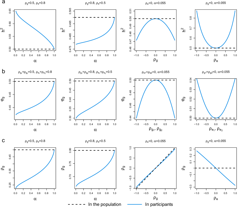
where is the density function of the standard normal distribution. Notably, is a monotonically decreasing function in (0,1) with , and . By definition, the heritability is the proportion of phenotypic variance explained by the genetic component. In (3), the denominator can be regarded as the variance of after selection, which is determined by the participation rate and the correlation between and . It is expected to shrink after selection. On the other hand, the numerator is more intricate as PB impacts both effect sizes of SNPs and the LD structure, and both contributes to the variance of the genetic component. Specifically, the term can be understood as the first-order contribution of the alterations in effect sizes to the genetic variance, and comes from the alterations in LD structures. The remaining terms involve the joint effects of the alterations in effect sizes of and the LD structure.
A comparison of and is shown in Figure 1(a). In general, with the other parameters fixed, the difference between and increases as decreases. It is worth noting that PB can lead to both upward and downward bias to the estimation of heritability in the sample of participants. For example, if the correlation between and arises solely from the genetic components, conditioning on participation will reduce the variance of the genetic component of in the selected sample. With the variance of the non-genetic component unchanged, the proportion of the genetic effects in the sample will shrink. Conversely, if the correlation between the phenotype and participation is induced by non-genetic factors only, the proportion of variance of attributed to the genetic component in the sample will increase, which leads to an upward bias in the estimation of heritability.
2.3 Genetic correlation estimated with participation bias
Here we consider two phenotypes, and , both following the additive model (1), and denotes their genetic correlation in the population. The corresponding genetic covariance is , where and are the heritability of the two phenotypes. Let , where and are per-standardized genetic effect sizes in the sample of participants, which maximize and , respectively. In parallel with , the quantity represents the “apparent” correlation between the genetic components of and that is being estimated ignoring PB. We show in Supplementary Note 1.3 that,
| (5) |
Here and are the covariance of with and ; and are the phenotypic correlations between and and , respectively, in the population. The heritabilities and in the denominator are derived in (3). We note that and in the denominator can be regarded as the shrunk phenotypic variance of and after selection. The term in the numerator is the first-order effects due to changes in the effect sizes of genetic variants from the population to the sample of participants. Furthermore, the term captures the effects due to the changes in the LD structure. The remaining terms in the numerator describe their combined effects.
Figure 1(b) shows the comparison of and . Similar to the results of heritability estimates, the bias induced by PB on genetic correlation increases when the participation rate decreases. The estimation of genetic correlation can have either upward or downward bias in the sample of participants.
2.4 Genetic correlation between participation and a phenotype
Intuitively, both genetic and non-genetic correlations between participation and the phenotype can lead to PB. The liability score underlying participation can be thought of as a special phenotype. We define , where is the per-standardized genetic effect sizes in the sample of participants, which maximizes . Note that the inside the expression of is the per-standardized genetic effect of in the population, which is not affected by PB. It can be shown that (see Supplementary Note 1.4)
| (6) |
Some comparisons between and are in Figure 1(c). Note that if there is no genetic correlation between the phenotype and participation in the population ( ), the correlation between genetic components in the sample will be in opposite direction of their phenotypic correlation, a form of collider bias.
2.5 Heritability and genetic correlation estimates with PB adjustment
With the results derived above, we provide a method to correct the effects of PB on the estimates of heritability and genetic correlations. Our method integrates two sources of information: i) the test statistics of participation derived from the IBD-based comparisons (ref.16); and ii) the mean shifts of other phenotypes from population to sample. Notably, although genotypes of non-participants are unavailable, population average of many phenotypes are available from sources such as census data. We start with showing how to adjust the estimate of genetic covariance and heritability here.
We define the mean shift of the standardized phenotype between the selected sample and the population as . We show that in model (1),
| (7) |
Given , is a monotonically increasing function of (Figure S1), the correlation of and and if .
In practice, we estimate the mean phenotypic value in both the sample of participants and another cohort that is representative of the population. The observed mean shift is just difference of the two estimates standardized (divided) by the standard deviation of the phenotypic values of the participants. Notably, while most of the mathematics have been derived for variables standardized in the population, phenotype mean shift is standardized with respect to the sample for convenience of application. For notations, we use , , , and to denote the estimates that are affected but not adjusted for PB, and the corresponding estimates after adjustments are denoted as , , , and . Based on (7), we derive the estimate of the phenotypic correlation between and :
| (8) |
By solving from (2) of Supplementary Note 1.4, we derive the adjusted genetic covariance of and :
| (9) |
where is the heritability of the participation liability score estimated with IBD-based method 16; is the estimated genetic covariance between and ignoring PB. By solving from (3) and substitute parameters with their estimates, the adjusted heritability estimate of is:
| (10) |
where is the estimated heritability of the phenotype ignoring PB. The adjusted genetic correlation of and is:
| (11) |
Similarly, we solve for from the approximation of in (18) in and Supplementary Note 1.3, and substitute parameters with their estimates, leading to:
| (12) | ||||
where is the estimated genetic covariance of and ignoring PB; and are the estimated genetic covariance of and and ignoring PB. The and are the estimated phenotypic correlation with participation for the two phenotypes derived with (8). The genetic correlation is then:
| (13) |
where the denominator is derived with (10).
The standard errors are estimated with a block jackknife procedure. In theory, if and are estimated accurately, the adjustment could even lead to a reduced variance, giving an estimate with both reduced bias and smaller standard error.
In practice, the heritability and genetic correlation are often estimated with marker-based methods such as LD score regression (LDSC). With random sampling, LDSC provides unbiased heritability and genetic covariance estimates 2; 18. In the selected sample, however, not only the SNP effects have changed due to PB, but also the LD structure. We show that the LDSC assumptions are violated in the selected sample, which leads to a negative bias to the estimate of (see Supplementary Note 1.5). Nevertheless, since this bias has an opposite direction relative to the bias resulting from assortative mating 5, the two sources of bias would partially cancel each other in real data applications. Currently, we believe that this bias resulting from the violation of the method’s assumption is negligible, and focus on the gap between and .
2.6 Simulations
Our simulation study has two goals. First, we validate our theoretical results on the effect of PB on estimates without adjustment. Second, we show that our adjustment reduces the impact of PB. We generated genetic data for unrelated participants (Methods). The genotypes were simulated from a binomial distribution with block-wise correlation structures. Three scenarios with high genetic correlation (), low genetic correlation (), and no genetic correlation () were examined. The non-genetic correlation was fixed at . The heritability of participation liability score was fixed at , and the participation rate () was set to , which matches the participation rate of the UKBB 7; 16. We used LDSC to estimate heritability and genetic correlation.
For heritability, when the true genetic correlation between participation and the related trait was , PB led to underestimation biases in heritability estimates for both scenarios with and . When the genetic correlation was or , PB resulted in overestimation bias (Table 1). As for the genetic correlation between two phenotypes other than participation (), we observed an overestimation bias when . The estimate of had an opposite sign when and (Table 2).
Then we applied our adjustment method to the estimates. With adjustments, both the heritability and genetic correlation are very close to the true value in the population, with standard errors comparable to those of the original estimates (Tables 1 and 2).For example, when and , the estimated heritability of in the sample of participants is 0.156 (SE=0.006). After our adjustment, the estimation is 0.199 (SE=0.010). The estimated genetic correlation between and is 0.503 (SE=0.050) before adjustment, and is 0.749 (SE=0.028) after adjustment. As for the genetic correlation between two other phenotypes, when , the estimated of is 0.218 (SE=0.029). After adjustment, the estimation is 0.502 (SE=0.027), with 0.5 as the true setting in the population.
| Theoretical | Simulated | Adjusted | True | Theoretical | Simulated | Adjusted | True |
| 0.156 | 0.156 (0.006) | 0.199 (0.010) | 0.2 | 0.504 | 0.503 (0.050) | 0.749 (0.028) | 0.75 |
| 0.230 | 0.229 (0.009) | 0.200 (0.011) | 0.2 | -0.063 | -0.059 (0.067) | 0.246 (0.062) | 0.25 |
| 0.254 | 0.254 (0.009) | 0.201 (0.011) | 0.2 | -0.273 | -0.270 (0.062) | -0.001 (0.066) | 0 |
| 0.465 | 0.469 (0.012) | 0.505 (0.016) | 0.5 | 0.624 | 0.636 (0.043) | 0.758 (0.029) | 0.75 |
| 0.544 | 0.549 (0.014) | 0.503 (0.016) | 0.5 | 0.084 | 0.084 (0.055) | 0.247 (0.054) | 0.25 |
| 0.563 | 0.568 (0.013) | 0.505 (0.017) | 0.5 | -0.141 | -0.141 (0.061) | -0.003 (0.064) | 0 |
| Setting | ||||
| Theoretical | Simulated | Adjusted | True | |
| 0.75 | 0.218 | 0.219 (0.029) | 0.502 (0.027) | 0.5 |
| 0.25 | 0.459 | 0.459 (0.024) | 0.498 (0.027) | 0.5 |
| 0 | 0.515 | 0.515 (0.023) | 0.500 (0.029) | 0.5 |
| 0.75 | -0.245 | -0.243 (0.053) | 0.202 (0.047) | 0.2 |
| 0.25 | 0.141 | 0.143 (0.029) | 0.200 (0.035) | 0.2 |
| 0 | 0.229 | 0.232 (0.028) | 0.203 (0.037) | 0.2 |
2.7 Real data applications on UKBB phenotypes
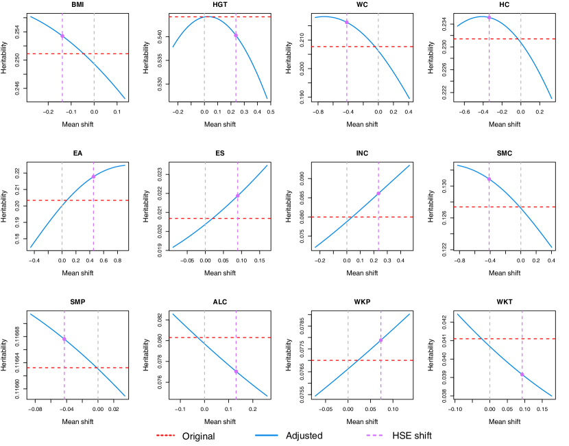
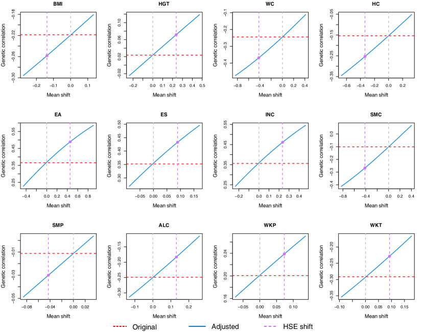
We applied our adjustment method to 12 UKBB phenotypes including 4 physical measures: body mass index (BMI), height (HGT), waist circumference (WC), and hip circumference (HC); 3 sociodemographic measures: educational attainment (EA), employment status (ES), and income (INC); and 5 lifestyle measures: current smoking status (SMC), previous smoking status (SMP), alcohol consumption (ALC), walking pace (WKP), and walking time (WKT). Detailed description of the data is summarized in Supplementary Note 1.6. We first estimated heritability and genetic correlations across the phenotypes ignoring PB. We also estimated their genetic correlation with participation based on the genome-wide association studies (GWAS) summary statistics derived from IBD-based information16. Then we calculated the mean shift between the UKBB and the Health Survey for England (HSE) dataset (Methods). We use the HSE dataset as a baseline as it incorporated the weighting to account for nonresponse bias.
Figures 2 and 3 show the effect of PB on the estimates of heritability and genetic correlation of the UKBB phenotypes as functions of mean shifts of the phenotypes. The adjusted estimates based on the observed mean shifts between UKBB and HSE data are indicated. Numerical results of the original (unadjusted) and adjusted estimates are shown in Table 3. With adjustments, the genetic components of BMI, WC, HC, EA, ES, INC, SMC, and WKP are significantly correlated with the genetic components of participation. Specifically, we found the heritability estimates have underestimation bias across those phenotypes that are genetically correlated with participation. Underestimation bias for unadjusted estimates is also observed for the absolute values of genetic correlations. In addition, we found that SMC, which previously lacked significant genetic correlation with participation (), surpassed the significance threshold of 0.05 with adjustment (). For ALC and WKT, the unadjusted results showed significant genetic correlation with participation ( and ). However, with adjustments, the estimated correlation shrunk and no longer statistically significant ( and ). We did not observe estimated correlations that switched signs with adjustment for those phenotypes.
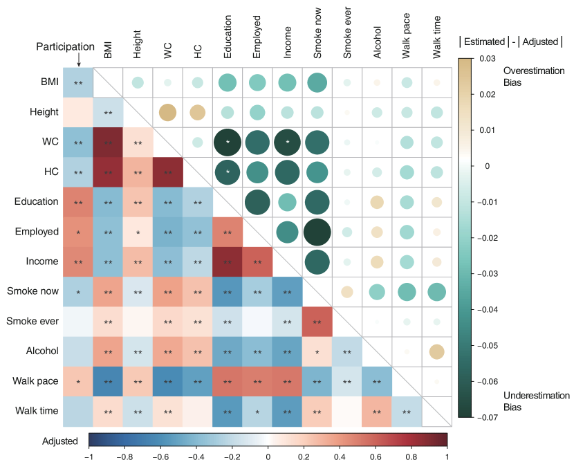
We further analyzed the genetic correlation of each pair of the 12 phenotypes (Figure 4). Compared with the original estimates, we did not observe estimates switching signs. Across phenotypes significantly correlated with participation, we found that, without adjustments, all the genetic correlation estimates had underestimation bias with respect to their absolute value. In addition, the adjusted genetic correlation estimates between WC and EA, HC and EA, and WC and INC, were significantly different from the unadjusted estimates with -values of , , and .
| Phenotype | ||||||
| Original | Adjusted | Original | Adjusted | Adjusted | ||
| BMI | -0.138 | 0.251 (0.012) | 0.253 (0.012) | -0.219 (0.073) | -0.258 (0.067) | -0.027 (0.012) |
| HGT | 0.237 | 0.544 (0.026) | 0.540 (0.026) | 0.024 (0.058) | 0.072 (0.059) | 0.154 (0.023) |
| WC | -0.419 | 0.208 (0.010) | 0.216 (0.010) | -0.244 (0.080) | -0.368 (0.058) | -0.173 (0.012) |
| HC | -0.336 | 0.231 (0.012) | 0.235 (0.012) | -0.153 (0.068) | -0.253 (0.056) | -0.148 (0.012) |
| EA | 0.438 | 0.203 (0.007) | 0.217 (0.008) | 0.366 (0.096) | 0.485 (0.068) | 0.160 (0.014) |
| ES | 0.089 | 0.021 (0.003) | 0.022 (0.002) | 0.352 (0.160) | 0.433 (0.139) | 0.023 (0.006) |
| INC | 0.235 | 0.080 (0.004) | 0.086 (0.004) | 0.356 (0.109) | 0.461 (0.086) | 0.076 (0.010) |
| SMC | -0.413 | 0.127 (0.008) | 0.131 (0.004) | -0.102 (0.086) | -0.267 (0.088) | -0.191 (0.009) |
| SMP | -0.043 | 0.117 (0.005) | 0.117 (0.003) | -0.011 (0.070) | -0.030 (0.070) | -0.020 (0.007) |
| ALC | 0.131 | 0.080 (0.004) | 0.077 (0.004) | -0.249 (0.091) | -0.183 (0.105) | 0.092 (0.008) |
| WKP | 0.073 | 0.077 (0.004) | 0.078 (0.003) | 0.201 (0.082) | 0.239 (0.077) | 0.014 (0.008) |
| WKT | 0.093 | 0.041 (0.003) | 0.039 (0.003) | -0.291 (0.119) | -0.228 (0.135) | 0.067 (0.008) |
† The mean shift between the phenotypes in the UKBB and HSE (UKBB minus HSE), which is calculated after rank-based inverse normal transformation, covariates correction, and standardization with UKBB standard deviations.
3 Discussion
In the last decade, many methods have been proposed to estimate heritability and genetic correlation. Despite the success, estimates are typically derived under the assumption of random sampling, without taking PB into account. In addition, the non-random component underlying participation is often implicitly thought of as a function of environmental factors and established phenotypes such as educational attainment, frequency of alcohol use, etc. Following this line of reasoning, to adjust for PB, a recent study15 applied IPW to the UKBB data, with a propensity score constructed from other phenotypes. Apart from the limitations that the propensity score was limited by the availability of phenotypes that could be harmonized between UKBB and other random sampling studies, most importantly, the propensity score does not include genotypes. For this IPW adjustment to be sufficient for analyses that include genotypes, the main focus of genetic studies that include heritability and genetic correlation estimates, it requires that the genetic component underlying participation manifests its effect entirely through the propensity score. Under this assumption, the participation polygenic score constructed in ref.16 (denoted as pPGS), based on a GWAS that did not use any information on other phenotypes, should not have any predictive power on other phenotypes conditioning on the propensity score. We examined this with four phenotypes, EA, BMI, and the invitation and participation in the secondary physical activity study. We observed significant associations (, Bonferroni correction) between pPGS and all four phenotypes before and after adjustment for the predicted participation indicated by the propensity score (Table 4), indicating that the assumption does not hold. Similar analyses were performed in ref.16 using EA in the place of the propensity score. These results suggest that participation should be treated as a complex behavioral trait in its own right with its specific genetic component, and not simply a consequence of other established phenotypes.
| Phenotypes | pPGS | pPGS adjusted for predicted participation | ||||
| Effect | -value | Sample size | Effect | -value | Sample size | |
| EA | 268,205 | 227,688 | ||||
| BMI | 270,330 | 227,688 | ||||
| Secondary invitation | 132,148/139,048 | 114,834/112,854 | ||||
| Secondary participation | 59,264/72,884 | 52,317/62,517 | ||||
In this article, we build a statistical model for understanding the influence of PB on estimating heritability and genetic correlation. We regard participation as a phenotype in its own right, which can be affected by a combination of genetic and non-genetic factors. Compared with the weighting strategy, our model utilizes the IBD-based information and provides extra degrees of freedom. We derived theoretical results for the expected differences between the heritability and genetic correlation estimates obtained from the biased sample and the actual values of the population. We directly model the GWAS summary statistics in the selected sample, without using the genotypic information of the non-participants. We validated the theoretical results with simulations and applied our results to 12 UKBB phenotypes. We found 8 of the phenotypes were significantly associated with participation of the UKBB. We also found that, without adjustments, the heritability and the absolute value of the genetic correlation estimates had underestimation bias in the sample of participants.
There are several limitations to the current approach. First, the IBD-based participation GWAS we used only captured direct effects, and we did not consider the indirect effects of participation. Second, the sample size of IBD siblings for deriving participation statistics is relatively limited. Although we have demonstrated via both simulations and real data applications that the standard errors before and after our adjustment are comparable, larger sample sizes will lead to more accurate results with smaller MSEs. Third, in order to adjust for PB, we leveraged the HSE dataset to derive the mean shift between UKBB and HSE. We assumed that the HSE dataset was based on random sampling, as it has incorporated weighting to account for nonresponse bias. Violation of this assumption would reduce the effectiveness of the adjustments, but most likely they would be in the right direction. Lastly, the adjustments were calculated assuming the invited list, about 9.5 million in size for the UKBB, is representative of the target population, about 21 million in size with the age constraint 13. Violation of this assumption does not affect the estimate of the genetic component underlying the overall participation bias that incorporates both invitation bias and agreeing to participate if invited bias. However, the estimate of the strength of this genetic component, its heritability, could be impacted, and through that affect the other adjustments. The exact effect is mathematically complicated and depends on many factors, but we can get an idea by considering two extreme scenarios for the UKBB study. One extreme is that all those who were not invited would not have agreed to participate if invited anyway. In this case, the appropriate adjustments would be smaller than what are currently estimated, the adjustment of heritability estimates for other phenotypes should be shrunk by about . The other extreme is if all the bias came from the invitation list, and participation upon invitation was completely random. In that case, our current adjustments would be in the right direction but conservative, smaller than what should be. Given that, we believe the adjustments we provided are reasonable. To do substantially better, more complicated modelling and additional information, such as phenotypic differences between target population and the invited list, are probably required.
Despite the limitations, our model and method provide insights about the genetic architecture underlying participation and other phenotypes. It is, we believe, an important first step towards adjusting PB in genetic studies in a way that does not rely entirely on phenotypic differences between sample and population. For future research, it is conceptually advantageous to develop statistical methods to investigate the underlying causality of participation and other phenotypes. In particular, it is often assumed that EA has a causal effect on participation 15, while whether and to what extent the inclination to participate, as a behavioral phenotype, has a causal impact on other phenotypes including EA remains unclear. A deeper understanding of causality will be helpful in understanding the underlying mechanisms and dynamics of human behavior.
4 Methods
4.1 Simulation settings
We simulated a population with sibling pairs and SNPs. The genotypes were generated from a binomial distribution with block-wise autoregressive (AR(1)) LD structure using the R package CorBin 19. Each block has SNPs, with the correlation matrix of the -th LD block as
| (1) |
where is the number of SNPs in the block, and Unif. The allele frequencies in each block were also sampled from Unif. The correlations are higher for adjacent variants and decrease with the increasing distance between the variants, which mimics the real LD structures 20. We set of the SNPs to have nonzero effects. Specifically, for the -th SNP with nonzero effects, and were simulated from a bivariate normal distribution with mean and variance and , with correlation . The non-genetic terms were also simulated from a bivariate normal distribution with mean , variance () and (), and correlation . For each time of the simulation, we generated the liability score of participation for each sample with , and another phenotype with , where is the standardized genotype. As for the analysis of two phenotypes, we generated the effect sizes of both phenotypes, as well as the effect sizes of participation liability score with a 3-dimensional normal distribution. We set the participation rate () and sibling recurrence risk () to and , which equals to the corresponding values reported in the UKBB 7; 21; 16. Samples with were selected as participants. We only included one of the sibling pairs, so the sample size of participants was around . We then performed GWAS on in the sample of participants. We followed the procedure in Benonisdottir and Kong (2023) to derive the test statistics of participation with IBD-based between-sib-pairs comparison information. Simulations were repeated 50 times.
4.2 UKBB summary statistics
The GWAS summary statistics of UKBB participation were directly downloaded from GWAS catalog 16. Other UKBB summary statistics based on the genetic data of 274,485 white British unrelated individuals in the UKBB after quality control 21. The phenotypes of interest were adjusted for year of birth (data-field 34), age at recruitment (data-field 21022), and sex (data-field 31) when applicable. We further adjusted top 40 principal components 21. Quantitative phenotypes except for EA, ALC, and WLP, were rank-based inverse normal transformed 22 separately for each sex. A detailed description of the process of phenotypes is provided in Supplementary Note 1.6. We used the same quality filtering protocol for the sequence variants as Benonisdottir and Kong (2023) 16. The analysis was restricted to the set of 500,632 high-quality variants with the missing rate and with MAF . We used PLINK 1.90 to derive GWAS summary statistics 23.
4.3 HSE datasets
We obtained the anthropometric measures from 81,118 individuals from the Health Survey for England (HSE) for the years 2006-2010 24; 25; 26; 27; 28, which consists of an annual cross-sectional survey. The samples are a representative population of England through a two-stage random probability sampling process 13. The HSE data have incorporated weighting to account for nonresponse bias since 2003 29. A detailed description of the collection of HSE datasets is in Supplementary Note 1.6. For the computation of the mean shift between HSE and UKBB, we restricted samples of white British ancestry and ages from 40 to 65, resulting in 20,208 individuals. The phenotypes in both HSE and UKBB were adjusted for sex, age, age2, sexage, and sexage2.
4.4 LD score regression
We used LD score regression (LDSC, v.1.0.1) to derive the estimates for heritability and genetic correlation, which ignores the effects of PB. In the simulations, the LD scores were computed with true LD matrices. The LD scores in real data analyses were computed by the Pan-UKB team 30 (downloaded on 7 April 2021).
4.5 Polygenic score analysis
We computed the pPGS with PLINK 1.90 23, which summed over the weighted genotypes of the SNPs after quality control. The scores were used as weights, which were transformed from the combined -values in the GWAS summary statistics of participation provided in ref. 16. The pPGS was standardized to have variance 1, and the relationship between the pPGS and EA, BMI, secondary invitation (binary), and secondary participation (binary) was estimated with a linear regression and logit regression in R (v.4.3.1), in the group of White British unrelateds. The sex, year of birth, age at recruitment, genotyping array, and 40 principal components were used as covariates.
5 Data availability
The GWAS summary statistics for participation are available on the GWAS catalog under the accession codes GCST90267221 and GCST90267223. The individual-level UKBB data can be applied on their website (http://www.ukbiobank.ac.uk/register-apply/).
6 Code availability
The replication codes are available at https://github.com/shuangsong0110/ParticipationBias.
7 Acknowledgements
This research has been conducted using the UK Biobank Resource (www.ukbiobank.ac.uk) under Application Number 68672.
8 Competing Interests
The authors declare that they have no competing interests.
References
- 1 Sudlow, C. et al. UK biobank: an open access resource for identifying the causes of a wide range of complex diseases of middle and old age. PLoS Medicine 12, e1001779 (2015).
- 2 Bulik-Sullivan, B. K. et al. LD score regression distinguishes confounding from polygenicity in genome-wide association studies. Nature Genetics 47, 291–295 (2015).
- 3 Kong, A. et al. The nature of nurture: Effects of parental genotypes. Science 359, 424–428 (2018).
- 4 Abdellaoui, A. & Verweij, K. J. Dissecting polygenic signals from genome-wide association studies on human behaviour. Nature Human Behaviour 5, 686–694 (2021).
- 5 Border, R. et al. Assortative mating biases marker-based heritability estimators. Nature Communications 13, 660 (2022).
- 6 Winship, C. & Mare, R. D. Models for sample selection bias. Annual Review of Sociology 18, 327–350 (1992).
- 7 Swanson, J. M. The UK Biobank and selection bias. The Lancet 380, 110 (2012).
- 8 Seaman, S. R. & White, I. R. Review of inverse probability weighting for dealing with missing data. Statistical Methods in Medical Research 22, 278–295 (2013).
- 9 van Alten, S., Domingue, B. W., Galama, T. J. & Marees, A. T. Reweighting the UK Biobank to reflect its underlying sampling population substantially reduces pervasive selection bias due to volunteering. medRxiv 2022–05 (2022).
- 10 Bisgard, K. M., Folsom, A. R., Hong, C.-P. & Sellers, T. A. Mortality and cancer rates in nonrespondents to a prospective study of older women: 5-year follow-up. American Journal of Epidemiology 139, 990–1000 (1994).
- 11 Manjer, J. et al. The malmö diet and cancer study: representativity, cancer incidence and mortality in participants and non-participants. European Journal of Cancer Prevention 489–499 (2001).
- 12 Drivsholm, T. et al. Representativeness in population-based studies: a detailed description of non-response in a Danish cohort study. Scandinavian Journal of Public Health 34, 623–631 (2006).
- 13 Fry, A. et al. Comparison of sociodemographic and health-related characteristics of uk biobank participants with those of the general population. American Journal of Epidemiology 186, 1026–1034 (2017).
- 14 Knudsen, A. K., Hotopf, M., Skogen, J. C., Øverland, S. & Mykletun, A. The health status of nonparticipants in a population-based health study: the Hordaland Health Study. American Journal of Epidemiology 172, 1306–1314 (2010).
- 15 Schoeler, T. et al. Participation bias in the UK Biobank distorts genetic associations and downstream analyses. Nature Human Behaviour 7, 1216–1227 (2023).
- 16 Benonisdottir, S. & Kong, A. Studying the genetics of participation using footprints left on the ascertained genotypes. Nature Genetics 55, 1413–1420 (2023).
- 17 Harville, D. A. Approximating the selection process. Biometrics 26, 51–66 (1970).
- 18 Ni, G. et al. Estimation of genetic correlation via linkage disequilibrium score regression and genomic restricted maximum likelihood. The American Journal of Human Genetics 102, 1185–1194 (2018).
- 19 Jiang, W., Song, S., Hou, L. & Zhao, H. A set of efficient methods to generate high-dimensional binary data with specified correlation structures. The American Statistician 75, 310–322 (2021).
- 20 Stephens, M. & Scheet, P. Accounting for decay of linkage disequilibrium in haplotype inference and missing-data imputation. The American Journal of Human Genetics 76, 449–462 (2005).
- 21 Bycroft, C. et al. The UK Biobank resource with deep phenotyping and genomic data. Nature 562, 203–209 (2018).
- 22 Beasley, T. M., Erickson, S. & Allison, D. B. Rank-based inverse normal transformations are increasingly used, but are they merited? Behavior Genetics 39, 580–595 (2009).
- 23 Chang, C. C. et al. Second-generation PLINK: rising to the challenge of larger and richer datasets. Gigascience 4, s13742–015 (2015).
- 24 National Centre for Social Research & University College London, Department of Epidemiology and Public Health. Health survey for England, 2006. [data collection] (2011). URL http://doi.org/10.5255/UKDA-SN-5809-1. SN: 5809.
- 25 National Centre for Social Research & University College London, Department of Epidemiology and Public Health. Health survey for England, 2007. [data collection] (2010). URL http://doi.org/10.5255/UKDA-SN-6112-1. SN: 6112.
- 26 National Centre for Social Research & University College London, Department of Epidemiology and Public Health. Health survey for England, 2008. [data collection] (2013). URL http://doi.org/10.5255/UKDA-SN-6397-2. SN: 6397.
- 27 National Centre for Social Research & University College London, Department of Epidemiology and Public Health. Health survey for England, 2009. [data collection] (2015). URL http://doi.org/10.5255/UKDA-SN-6732-2. SN: 6732.
- 28 National Centre for Social Research & University College London, Department of Epidemiology and Public Health. Health survey for England, 2010. [data collection] (2015). URL http://doi.org/10.5255/UKDA-SN-6986-3. SN: 6986.
- 29 National Centre for social research health survey for England 2003. Volume 3. Methodology and documentation London, United Kingdom: Department of health; 2004. https://webarchive.nationalarchives.gov.uk/ukgwa/20121206162012/http://www.dh.gov.uk/prod_consum_dh/groups/dh_digitalassets/@dh/@en/documents/digitalasset/dh_4098912.pdf. Published December 17, 2004. Accessed December 22, 2015.
- 30 Pan-UKB team. https://pan.ukbb.broadinstitute.org. 2020.