On adaptive stochastic extended iterative methods for solving least squares

Abstract.

In this paper, we propose a novel adaptive stochastic extended iterative method, which can be viewed as an improved extension of the randomized extended Kaczmarz (REK) method, for finding the unique minimum Euclidean norm least-squares solution of a given linear system. In particular, we introduce three equivalent stochastic reformulations of the linear least-squares problem: stochastic unconstrained and constrained optimization problems, and the stochastic multiobjective optimization problem. We then alternately employ the adaptive variants of the stochastic heavy ball momentum (SHBM) method, which utilize iterative information to update the parameters, to solve the stochastic reformulations. We prove that our method converges linearly in expectation, addressing an open problem in the literature related to designing theoretically supported adaptive SHBM methods. Numerical experiments show that our adaptive stochastic extended iterative method has strong advantages over the non-adaptive one.

1. Introduction

Large-scale linear systems arise in many areas of scientific computing and engineering, including computerized tomography [36], machine learning [10], signal processing [8], etc. In this paper, we consider solving the linear system

(1) $$Ax=b,\ A\in\mathbb{R}^{m\times n},\ b\in\mathbb{R}^{m}$$

in the least-squares sense, i.e., finding $x^{*}$ such that

(2) $$x^{*}\in\arg\min\{\|Ax-b\|^{2}_{2},x\in\mathbb{R}^{n}\}.$$

It is well-known [16, 6, 12] that the problem (2) has a unique minimum Euclidean norm least-squares solution $A^{\dagger}b$, where $A^{\dagger}$ denotes the Moore-Penrose pseudoinverse of $A$.

The randomized Kaczmarz (RK) method [54] has recently gained popularity in solving large-scale linear systems for its reduced iteration cost and low memory storage requirements. If the linear system (1) is consistent, the RK method converges to $A^{\dagger}b$ linearly in expectation with an appropriate initial point [54, 20, 13]. If it is inconsistent, however, Needell [39] showed that the RK method only converges within a radius (convergence horizon) of the least-squares solution; see also [4, 33] for some further comments.

To address this issue, Zouzias and Freris [62] applied a modification to the RK method, proposing the randomized extended Kaczmarz (REK) method. Letting $\text{Range}(A)$ represent the range space of $A$ and $b_{\text{Range}(A)}$ denote the orthogonal projection of $b$ on $\operatorname{Range}(A)$, it is known that (2) is equivalent to solving the consistent system $Ax=b_{\text{Range}(A)}$ [22]. Therefore, the REK method first uses random projection to obtain a vector $z^{k+1}$ that approximates the projection of $b$ onto the orthogonal complement space of $\operatorname{Range}(A)$, ensuring that $b-z^{k+1}\approx b_{\operatorname{Range}(A)}$, and then applies one RK iteration to solve the linear system $Ax=b-z^{k+1}$. In this paper, we employ the same procedure to propose a more general framework. Furthermore, we also intend to incorporate the heavy ball momentum (HBM) [45, 15] into the REK-type method to enhance its performance. To the best of our knowledge, this is the first study to investigate the momentum variants of the REK-type method.

Specifically, our stochastic extended iterative method with adaptive HBM adopts the following iteration scheme:

(3) $$\left\{\begin{array}[]{ll}z^{k+1}=z^{k}-\mu_{k}AT_{k}T_{k}^{\top}Az^{k}+\omega_{k}(z^{k}-z^{k-1}),\\ x^{k+1}=x^{k}-\alpha_{k}A^{\top}S_{k}S_{k}^{\top}(Ax^{k}-(b-z^{k+1}))+\beta_{k}(x^{k}-x^{k-1}),\end{array}\right.$$

where random matrices $S_{k}$ and $T_{k}$ are drawn from user-defined probability spaces $(\Omega,\mathcal{F},P)$ and $(\overline{\Omega},\overline{\mathcal{F}},\overline{P})$, respectively, $\mu_{k}$ and $\alpha_{k}$ are the step-sizes, and $\omega_{k}$ and $\beta_{k}$ are the momentum parameters. We note that by manipulating the probability spaces, our algorithmic framework can recover a wide range of popular algorithms, including the REK method and its variants; see Remark 3.2 for further discussion.

1.1. Our contributions

In this paper, we present a simple and versatile stochastic extended iterative algorithmic framework for finding the unique minimum Euclidean norm least-squares solution of any linear systems. The main contributions of this work are as follows.

• We introduce a novel scheme to reformulate any least-squares problem into several seemingly different but equivalent forms, including the augmented linear system [1, 4], the unconstrained and constrained stochastic optimization problem, and the multiobjective optimization problem. This reformulation enables us to establish new connections between these problems. Moreover, we identify the conditions that ensure these reformulations share the same solution set.

• It is well-known that one of the limitations of the HBM method is its dependence on prior knowledge of certain problem parameters, such as singular values of a certain matrix [29, 20, 15, 7]. If $Ax=b$ is consistent, there have been works on the strategy to adaptively learn the parameters in the stochastic HBM (SHBM) method, such as the adaptive SHBM (ASHBM) method [60] and the adaptive Bregman-Kaczmarz method [31, 59]. However, these strategies cannot be directly applied to general cases of the least-square problems. In this paper, we address the issues brought by inconsistency and extend such adaptive strategies, proposing the adaptive stochastic extended iterative method. To the best of our knowledge, this is the first time that adaptive HBM is integrated for solving the least-squares problem (2) without assuming the consistency of the corresponding linear system $Ax=b$.

• We demonstrate that our method converges linearly in expectation to the unique minimum Euclidean norm least-squares solution $A^{\dagger}b$. Furthermore, as our results hold for a broad range of probability spaces $(\Omega,\mathcal{F},P)$ and $(\overline{\Omega},\overline{\mathcal{F}},\overline{P})$, one can develop new and efficient variants of the method tailored to handle problems with specific structures by designing appropriate probability spaces. Numerical experiments are also provided to confirm our results.

1.2. Related work

1.2.1. Stochastic reformulation of linear systems

In the seminal paper [49], Richtárik and Takáš introduced the concept of stochastic reformulation of consistent linear systems. This approach, offering multiple equivalent interpretations, can serve as a platform for researchers from various communities to leverage their domain-specific insights. Specifically, their reformulation includes as a stochastic optimization problem, a stochastic linear system, a stochastic fixed point problem, and a stochastic intersection problem. They explored methods including stochastic gradient descent, stochastic Newton’s method, stochastic proximal point method, stochastic fixed point method, and stochastic projection method, demonstrating that these methods are equivalent when applied to the corresponding reformulations. However, the inclusion of the Moore-Penrose inverse in their reformulations would make the associated algorithm difficult to parallelize.

Recently, Zeng et al. [60] proposed a novel scheme to reformulate consistent linear system into a stochastic problem and employed the SHBM to solve the associated problem, where parallel computing is able to be applied. Subsequently, Lorenz and Winkler [31] adopted this idea and developed the minimal error momentum Bregman-Kaczmarz method to find a solution to the linear system with certain properties, such as sparsity. However, all of stochastic reformulations mentioned above are based on the assumption that the linear system is consistent. This paper goes beyond this limitation and develop a family of stochastic reformulations for arbitrary linear systems (consistent or inconsistent, overdetermined or underdetermined, full-rank or rank-deficient). To the best of our knowledge, this is the first study that addresses the reformulation of any linear system into a stochastic problem.

1.2.2. The Kacmzarz method

The Kaczmarz method [25], also known as algebraic reconstruction technique (ART) [23, 17], is a classic yet effective row-action iteration solver for the linear system. Starting from $x^{0}\in\mathbb{R}^{n}$, the Kaczmarz method constructs $x^{k+1}$ by

$$x^{k+1}=x^{k}-\frac{A_{i_{k},:},x^{k}-b_{i_{k}}}{\|A_{i_{k},:}\|^{2}_{2}}A_{i_{k},:}^{\top},$$

where $A_{i_{k},:}$ denotes the $i_{k}$-th row of $A$, $b_{i_{k}}$ denotes the $i_{k}$-th entry of $b$, and ${i_{k}}$ is cyclically selected from $[m]:=\{1,\cdots,m\}$. The iteration sequence $\{x^{k}\}_{k\geq 0}$ converges to a certain solution but the convergence rate is hard to obtain. In the seminal paper [54], Strohmer and Vershynin studied the RK method and proved that when the linear system is consistent, RK converges linearly in expectation. Since then, there is a large amount of work on the development of the Kaczmarz-type methods including accelerated RK methods [28, 21, 29, 60], randomized Douglas-Rachford methods [20], block Kaczmarz methods [38, 41, 34, 19], greedy RK methods [2, 18], etc. As mentioned above, Zouzias and Freris [62] proposed the REK algorithm for the cases when the linear system $Ax=b$ is inconsistent. Subsequently, there is a large amount of work on the development of the REK-type methods, including its block or deterministic variants [57, 42, 13, 12, 58, 56, 46, 47, 3], greedy randomized augmented Kaczmarz (GRAK) method [4], randomized extended Gauss-Seidel (REGS) method [11, 33], etc.

Our particular interest lies in the randomized extended average block Kaczmarz (REABK) method proposed by Du et al. [12]. Let $\left\{\mathcal{I}_{1},\mathcal{I}_{2},\dots,\mathcal{I}_{\ell}\right\}$ and $\left\{\mathcal{J}_{1},\mathcal{J}_{2},\dots,\mathcal{J}_{t}\right\}$ be partitions of $[m]$ and $[n]$, respectively. We use $A_{:,\mathcal{J}_{j_{k}}}$ and $A_{\mathcal{I}_{i_{k}},:}$ to denote the column and row submatrix of $A$ indexed by $\mathcal{J}_{j_{k}}$ and $\mathcal{I}_{i_{k}}$, respectively. Inspired by the randomized average block Kaczmarz (RABK) method proposed by Necoara [38], Du et al. [12] introduced the following REABK method:

(4) $$z^{k+1} =z^{k}-\frac{\alpha}{\|A_{:,\mathcal{J}_{j_{k}}}\|_{F}^{2}}A_{:,\mathcal{J}_{j_{k}}}A_{:,\mathcal{J}_{j_{k}}}^{\top}z^{k},$$

$$x^{k+1} =x^{k}-\frac{\alpha}{\|A_{\mathcal{I}_{i_{k}},:}\|_{F}^{2}}A_{\mathcal{I}_{i_{k}},:}^{\top}(A_{\mathcal{I}_{i_{k}},:}x^{k}-b_{\mathcal{I}_{i_{k}}}+z^{k+1}_{\mathcal{I}_{i_{k}}}),$$

where $\alpha$ is the step-size. Particularly, if the partition parameters $\ell=m$, $t=n$, and the step-size $\alpha=1$, then REABK reduces to the REK method [62]. The REABK method is able to be parallelized, but its effectiveness can be limited by the choice of step-size $\alpha$, which depends on the singular values of the submatrices involved [12, Theorem 2.7]. Indeed, adopting an adaptive strategy for the step-size is often more beneficial in practical applications [38]. The authors provided an adaptive choice for the step-size of REABK in [56]. In this paper, we introduce a strategy for choosing adaptive step-sizes applicable to a broad range of stochastic extended iterative methods. Furthermore, our convergence analysis is more comprehensive, leading to an improved convergence factor.

In addition, we note that the RK method can be seen as a variant of the SGD method [20, 40, 40, 32, 61]. To solve the optimization problem $\min f(x):=\frac{1}{m}\sum_{i=1}^{m}f_{i}(x)$, SGD employs the following update rule

(5) $$x^{k+1}=x^{k}-\alpha_{k}\nabla f_{i_{k}}(x^{k}),$$

where $\alpha_{k}$ is the step-size and $i_{k}$ is selected randomly. If the objective function $f(x)=\frac{1}{2m}\|Ax-b\|^{2}_{2}=\frac{1}{2m}\sum_{i=1}^{m}(A_{i,:}x-b_{i})^{2}$, then SGD reduces to the RK method.

1.2.3. Momentum acceleration

Building upon the success of the HBM method, various recent studies aim to extend this acceleration technique to the SGD method [29, 5, 53, 21, 48, 30, 35]. The resulting method is called the stochastic HBM (SHBM) method. Specifically, a heavy ball momentum term, $\beta_{k}(x^{k}-x^{k-1})$, is incorporated into the SGD method (5), leading to the iteration scheme $x^{k+1}=x^{k}-\alpha_{k}\nabla f_{i_{k}}(x^{k})+\beta_{k}(x^{k}-x^{k-1}).$ However, the parameters $\alpha_{k}$ and $\beta_{k}$ for this method may rely on certain problem parameters that are generally inaccessible. For instance, the choices of $\alpha_{k}$ and $\beta_{k}$ for the SHBM method [29, 45, 15, 7] for solving the linear system $Ax=b$ require knowledge of the largest singular value as well as the smallest nonzero singular value of matrix $A$. Hence, it is an open problem whether one can design a theoretically supported adaptive SHBM method [5, 7]. For certain types of problems, some recent works have provided answers to this question [50, 5, 60, 59, 31, 24].

Our result is closely related to the work [60], where an adaptive SHBM (ASHBM) was developed to solve the stochastic problem reformulated from consistent linear systems. It was demonstrated that ASHBM exhibits convergence bound that is at least as that of the non-momentum method. Actually, the strategy for adaptively updating the iterate $z^{k+1}$ in our stochastic extended iterative method with HBM is inspired by this ASHBM. However, our adaptive strategy for updating $x^{k+1}$ is distinct from the aforementioned works.

1.3. Notations

For any random variable $\xi$, let $\mathbb{E}[\xi]$ denote its expectation. For any matrix $A\in\mathbb{R}^{m\times n}$, we use $A_{i,:}$, $A_{:,j}$, $A^{\top}$, $A^{\dagger}$, $\|A\|_{F}$, $\sigma_{\max}(A)$, $\sigma_{\min}(A)$, $\text{rank}(A)$, $\text{Range}(A)$, and $\text{Range}(A)^{\perp}$ to denote the $i$-th row, the $j$-th column, the transpose, the Moore-Penrose pseudoinverse, the Frobenius norm, the largest singular value, the smallest nonzero singular value, the rank, the range space, and the orthogonal complement space of the range space of $A$, respectively. When $A$ is symmetric and positive semidefinite, we use $\lambda_{\max}(A)$ and $\lambda_{\min}(A)$ to denote the largest eigenvalue, and the smallest nonzero eigenvalue of $A$, respectively. Given $\mathcal{J}\subseteq[m]:=\{1,\ldots,m\}$, the complementary set of $\mathcal{J}$ is denoted by $\mathcal{J}^{c}$, i.e. $\mathcal{J}^{c}=[m]\setminus\mathcal{J}$. We use $A_{\mathcal{J},:}$ and $A_{:,\mathcal{J}}$ to denote the row and column submatrix indexed by $\mathcal{J}$, respectively. For any vector $b\in\mathbb{R}^{m}$, we use $b_{i}$, $\|b\|_{2}$, and $b_{\text{Range}(A)}$ to denote the $i$-th entry, the Euclidean norm, and the orthogonal projection onto $\text{Range}(A)$ of $b$, respectively. The identity matrix and the unit vector are denoted by $I$ and $e_{i}$, respectively.

1.4. Organization

The remainder of the paper is organized as follows. In Section 2, we investigate stochastic reformulations of the least-squares problem. Section 3 and Section 4 describe the stochastic extended iterative method and its momentum variant, respectively. Section 5 reports the mentioned numerical experiments and Section 6 concludes the paper. Proofs of all main results are provided in the appendix.

2. Stochastic reformulation of the least-squares problem

In this section, we will present several equivalent reformulations of the least-squares problem (2).

Augmented linear system. It is well-known that the least-squares problem (2) can be transformed equivalently into solving the following consistent augmented linear system [1, 4]

(6) $$\left\{\begin{array}[]{ll}A^{\top}z=0,\\ Ax=b-z,\end{array}\right.$$

which can also be written in the form of the augmented matrix

$$\begin{bmatrix}I&A\\ A^{\top}&0\end{bmatrix}\begin{bmatrix}z\\ x\end{bmatrix}=\begin{bmatrix}b\\ 0\end{bmatrix}\Leftrightarrow\tilde{A}\tilde{x}=\tilde{b}.$$

Unconstrained stochastic optimization problem. We now consider the following least-square problem for the augmented linear system

$$\min_{\tilde{x}\in\mathbb{R}^{m+n}}\Phi(\tilde{x}):=\frac{1}{2}\|\tilde{A}\tilde{x}-\tilde{b}\|_{2}^{2}.$$

Just as the sketching strategy applied in [19, 60], we take on a special sketching matrix $\tilde{S}=\begin{bmatrix}S&0\\ 0&T\end{bmatrix}$, where random matrices $S$ and $T$ are drawn from probability spaces $(\Omega,\mathcal{F},P)$ and $(\overline{\Omega},\overline{\mathcal{F}},\overline{P})$, respectively. We can arrive at the following unconstrained stochastic optimization problem

(7) $$\min\limits_{(x,z)\in\mathbb{R}^{n}\times\mathbb{R}^{m}}\Phi(x,z):=\mathbb{E}\left[\Phi_{S,T}(x,z)\right],$$

where $\Phi_{S,T}(x,z):=\frac{1}{2}\|T^{\top}A^{\top}z\|_{2}^{2}+\frac{1}{2}\|S^{\top}(Ax-(b-z))\|^{2}_{2}.$

Constrained stochastic optimization problem. Let

(8) $$g_{T}(z):=\frac{1}{2}\|T^{\top}A^{\top}z\|_{2}^{2},\ \ f_{S}(x,z):=\frac{1}{2}\|S^{\top}(Ax-(b-z))\|^{2}_{2},$$

and

(9) $$g(z):=\mathbb{E}_{T\in\overline{\Omega}}\left[g_{T}(z)\right],\ \ f(x,z):=\mathbb{E}_{S\in\Omega}\left[f_{S}(x,z)\right].$$

We also consider the following constrained stochastic optimization problem

(10) $$\text{Find}\ x,z\ \ \text{subject to}\ g(z)=0,\ f(x,z)=0.$$

Multiobjective optimization problem. Consider the vector-valued function $\Psi_{S,T}:\mathbb{R}^{n}\times\mathbb{R}^{m}\to\mathbb{R}\times\mathbb{R}$ defined by $\Psi_{S,T}(x,z):=\left(g_{T}(z),f_{S}(x,z)\right)$. Let $\Psi(x,z):=\mathbb{E}[\Psi_{S,T}(x,z)]=\left(g(z),f(x,z)\right)$. The associated unconstrained multiobjective optimization problem is defined as

(11) $$\min\limits_{(x,z)\in\mathbb{R}^{n}\times\mathbb{R}^{m}}\Psi(x,z).$$

In most cases, it is impossible to find a single point that minimizes all objective functions at once, so it is necessary to consider the concept of Pareto optimality. We refer the reader to [51, 14, 55] for more details about the multiobjective optimization problem. However, we can find a single point that minimizes all objective functions for (11). Indeed, since $g(z)\geq 0$ and $f(x,z)\geq 0$, and $g(A^{\dagger}b)=0$ and $f(A^{\dagger}b,b_{\text{Range}(A)^{\perp}})=0$, we know that $(A^{\dagger}b,b_{\text{Range}(A)^{\perp}})$ can minimize all objective functions for the multiobjective optimization problem (11).

2.1. Equivalent expressions of the stochastic reformulations

For convenience, we use $\mathcal{X}_{\Phi}$, $\mathcal{X}_{g,f}$, and $\mathcal{X}_{\Psi}$ to denote the sets of minimizers for the unconstrained stochastic optimization problem (7), the constrained stochastic optimization problem (10), and the multiobjective optimization problem (11), respectively. We have the following theorem which establishes the equivalence between these three stochastic formulations.

Theorem 2.1.

For any probability spaces $(\Omega,\mathcal{F},P)$ and $(\overline{\Omega},\overline{\mathcal{F}},\overline{P})$, we have $\mathcal{X}_{\Phi}=\mathcal{X}_{g,f}=$ $\mathcal{X}_{\Psi}$.

Proof.

It can be verified that $(A^{\dagger}b,b_{\text{Range}(A)^{\perp}})$ belongs to both $\mathcal{X}_{\Phi}$ and $\mathcal{X}_{g,f}$, which implies that both of them are nonempty. Since $\Phi(A^{\dagger}b,b_{\text{Range}(A)^{\perp}})=0$, we know that

$$\left(\overline{x},\overline{z}\right)\in\mathcal{X}_{\Phi}\Leftrightarrow\Phi\left(\overline{x},\overline{z}\right)=0\Leftrightarrow\left\{\begin{array}[]{ll}\mathbb{E}_{T\in\overline{\Omega}}\left[\frac{1}{2}\left\|T^{\top}A^{\top}\overline{z}\right\|_{2}^{2}\right]=0,\\ \mathbb{E}_{S\in\Omega}\left[\frac{1}{2}\left\|S^{\top}(A\overline{x}-(b-\overline{z}))\right\|^{2}_{2}\right]=0,\end{array}\right.\Leftrightarrow\left\{\begin{array}[]{ll}g(\overline{z})=0,\\ f(\overline{x},\overline{z})=0,\end{array}\right.$$

which implies that $\mathcal{X}_{\Phi}=\mathcal{X}_{g,f}=$ $\mathcal{X}_{\Psi}$. This completes the proof of the theorem. ∎

2.2. Exactness of the reformulations

In this subsection, we examine the exactness of the reformulations. By exactness, we mean that $x^{*}$ is a solution to (2) if and only if there exists a $z^{*}$ such that $(x^{*},z^{*})$ is a minimizer of the reformulated problem. We define

(12) $$M:=\mathbb{E}_{S\in\Omega}[SS^{\top}],\ \ \overline{M}:=\mathbb{E}_{T\in\overline{\Omega}}[TT^{\top}],$$

and

(13) $$\mathcal{S}:=\{y\in\mathbb{R}^{m}\mid M^{\frac{1}{2}}y\in M^{\frac{1}{2}}\left(b+\text{Range}(A)\right),y\in\text{Null}(A\overline{M}A^{\top})\}.$$

We have the following result which provides a necessary and sufficient condition for the stochastic reformulations (7) to be exact. For convenience, we use $\mathcal{X}_{\text{aug}}$ to denote the set of solutions for the augmented linear system (6).

Theorem 2.2.

Suppose that $M$ and $\mathcal{S}$ are defined by (12) and (13), respectively. Then $\mathcal{X}_{\Phi}=\mathcal{X}_{\text{aug}}$ if and only if $\mathcal{S}=b_{\text{Range}(A)^{\perp}}$ and $\text{Null}\left(A^{\top}MA\right)=\text{Null}(A)$.

Proof.

Since $\mathcal{X}_{\text{aug}}=\{(x,z)\mid A^{\top}z=0,Ax=b-z\}$, we know that for any $\left(\tilde{x},\tilde{z}\right)\in\mathcal{X}_{\text{aug}}$, it holds that $\tilde{z}\in\text{Null}(A^{\top})\cap\left(b+\text{Range}(A)\right)$. Note that

(14) $$\text{Null}(A^{\top})\cap\left(b+\text{Range}(A)\right)=\text{Range}(A)^{\perp}\cap\left(b+\text{Range}(A)\right)=b_{\text{Range}(A)^{\perp}},$$

which implies that $\tilde{z}=b_{\text{Range}(A)^{\perp}}$. Hence, $\mathcal{X}_{\text{aug}}$ can be rewritten as $\mathcal{X}_{\text{aug}}=\{(x,b_{\text{Range}(A)^{\perp}})\mid Ax=b_{\text{Range}(A)}\}.$ Furthermore, according to the proof of Theorem 2.1, for any $\left(\overline{x},\overline{z}\right)\in\mathcal{X}_{\Phi}$, it holds that

$$(\overline{x},\overline{z})\in\mathcal{X}_{\Phi} \Leftrightarrow\left\{\begin{array}[]{ll}g(\overline{z})=0\\ f(\overline{x},\overline{z})=0\end{array}\right.\Leftrightarrow\left\{\begin{array}[]{ll}\overline{M}^{\frac{1}{2}}A^{\top}\overline{z}=0\\ M^{\frac{1}{2}}A\overline{x}=M^{\frac{1}{2}}(b-\overline{z})\end{array}\right.\Leftrightarrow\left\{\begin{array}[]{ll}\overline{z}\in\text{Null}\left(A\overline{M}A^{\top}\right),\\ M^{\frac{1}{2}}\overline{z}\in M^{\frac{1}{2}}\left(b+\text{Range}(A)\right),\\ M^{\frac{1}{2}}A\overline{x}=M^{\frac{1}{2}}(b-\overline{z}).\end{array}\right.$$

Consequently, we can get that $\mathcal{X}_{\Phi}=\mathcal{X}_{\text{aug}}$ if and only if

$$\left\{\begin{array}[]{ll}\mathcal{S}=b_{\text{Range}(A)^{\perp}},\\ \{x\in\mathbb{R}^{n}\mid Ax=b_{\text{Range}(A)}\}=\{x\in\mathbb{R}^{n}\mid M^{\frac{1}{2}}Ax=M^{\frac{1}{2}}b_{\text{Range}(A)}\},\end{array}\right.$$

i.e., $\mathcal{S}=b_{\text{Range}(A)^{\perp}}$ and $\text{Null}\left(A^{\top}MA\right)=\text{Null}(A)$. ∎

Remark 2.3.

By combining Theorems (2.1) and (2.2), we can conclude that $\mathcal{X}_{\Phi}=\mathcal{X}_{g,f}=\mathcal{X}_{\Psi}=\mathcal{X}_{\text{aug}}$ if and only if $\mathcal{S}=b_{\text{Range}(A)^{\perp}}$ and $\text{Null}\left(A^{\top}MA\right)=\text{Null}(A)$.

From the proof of Theorem 2.2, we know that $x^{*}$ is a solution to the least-squares problem (2) if and only if $(x^{*},b_{\text{Range}(A)^{\perp}})\in\mathcal{X}_{\text{aug}}$. Hence, Theorem 2.2 present a necessary and sufficient condition for the reformulations to be exact. Next, we provide a sufficient condition for the exactness.

Corollary 2.4.

If $\overline{M}=\mathbb{E}_{T\in\overline{\Omega}}\left[TT^{\top}\right]$ and $M=\mathbb{E}_{S\in\Omega}\left[SS^{\top}\right]$ are positive definite matrices, then the stochastic reformulations (7), (10), and (11) are exact.

Proof.

Now we have $\mathcal{S}=\left\{y\in\mathbb{R}^{m}\mid y\in\text{Null}(A^{\top}),y\in b+\text{Range}(A)\right\}=b_{\text{Range}(A)^{\perp}}$, where the last equality follows from (14). Since $\text{Null}\left(A^{\top}MA\right)=\text{Null}(A)$, by Remark 2.3, we can conclude that this corollary holds. ∎

In this paper, we make the following assumption on the probability spaces $(\overline{\Omega},\overline{\mathcal{F}},\overline{P})$ and $(\Omega,\mathcal{F},P)$.

Assumption 2.1.

Let $(\overline{\Omega},\overline{\mathcal{F}},\overline{P})$ and $(\Omega,\mathcal{F},P)$ be the probability spaces from which the sampling matrices are drawn. We assume that $\mathbb{E}_{T\in\overline{\Omega}}\left[TT^{\top}\right]$ and $\mathop{\mathbb{E}}_{S\in\Omega}\left[SS^{\top}\right]$ are positive definite matrices. Additionally, we assume that the sampling space $\Omega$ is finite.

Corollary 2.4 implies that Assumption 2.1 serves as a sufficient condition for the stochastic reformulations (7), (10), and (11) to be exact. Additionally, the assumption regarding the finity of the sampling space $\Omega$ is necessary to ensure that a certain parameter remains bounded, as shown in (22).

3. Stochastic extended iterative methods with adaptive step-sizes

In this section, we consider employing the stochastic gradient descent (SGD) with adaptive step-sizes to solve those stochastic reformulations of the linear system (1). Specifically, let $z^{0}\in b+\text{Range}(A)$ and $x^{0}\in\text{Range}(A^{\top})$ be the initial points, our stochastic extended iterative method alternately minimizes $g(z)$ and $f(x,z)$ in (9) and the scheme can be written as

(15) $$z^{k+1} =z^{k}-\mu_{k}\nabla g_{T_{k}}(z^{k})=z^{k}-\mu_{k}AT_{k}T_{k}^{\top}A^{\top}z^{k},$$

$$x^{k+1} =x^{k}-\alpha_{k}\nabla_{x}f_{S_{k}}(x^{k},z^{k+1})=x^{k}-\alpha_{k}A^{\top}S_{k}S_{k}^{\top}(Ax^{k}-(b-z^{k+1})),$$

where $T_{k}$ and $S_{k}$ are drawn from the sample space $\overline{\Omega}$ and $\Omega$, respectively, and $\mu_{k}$ and $\alpha_{k}$ are the step-sizes. Specifically, the step-size $\mu_{k}$ is chosen as

(16) $$\mu_{k}=\left\{\begin{array}[]{ll}(2-\eta)\overline{L}_{\text{adap}}^{(k)},&\text{if}\;T_{k}^{\top}A^{\top}z^{k}\neq 0;\\ 0,&\text{otherwise},\end{array}\right.$$

where

(17) $$\overline{L}_{\text{adap}}^{(k)}:=\frac{\|T_{k}^{\top}A^{\top}z^{k}\|_{2}^{2}}{\|AT_{k}T_{k}^{\top}A^{\top}z^{k}\|_{2}^{2}},$$

and $\eta\in(0,2)$ is the relaxation parameter for adjusting the step-size $\mu_{k}$. The step-size $\alpha_{k}$ is chosen as

(18) $$\alpha_{k}=\left\{\begin{array}[]{ll}(2-\zeta)L_{\text{adap}}^{(k)},&\text{if}\;S_{k}^{\top}\left(Ax^{k}-(b-z^{k+1})\right)\neq 0;\\ 0,&\text{otherwise},\end{array}\right.$$

where

(19) $$L_{\text{adap}}^{(k)}:=\frac{\left\|S_{k}^{\top}\left(Ax^{k}-(b-z^{k+1})\right)\right\|_{2}^{2}}{\left\|A^{\top}S_{k}S_{k}^{\top}\left(Ax^{k}-(b-z^{k+1})\right)\right\|_{2}^{2}},$$

and $\zeta\in(0,2)$ is the relaxation parameter for adjusting the step-size $\alpha_{k}$. The following lemma ensures that the step-sizes $\mu_{k}$ and $\alpha_{k}$ are well-defined.

Lemma 3.1 ([60], Lemma 2.3).

Assume that the linear system $Ax=b$ is consistent. Then for any matrix $S\in\mathbb{R}^{m\times q}$ and any vector $\tilde{x}\in\mathbb{R}^{n}$, it holds that $A^{\top}SS^{\top}(A\tilde{x}-b)\neq 0$ if and only if $S^{\top}(A\tilde{x}-b)\neq 0$.

From Lemma 3.1 and the consistency of $A^{\top}z=0$ and $Ax=b-z^{k+1}$, we know that both $\overline{L}_{\text{adap}}^{(k)}$ and $L_{\text{adap}}^{(k)}$ are well-defined, ensuring that the step sizes are also well-defined. This is because $T_{k}^{\top}A^{\top}z^{k}\neq 0$ implies that $AT_{k}T_{k}^{\top}A^{\top}z^{k}\neq 0$, and $S_{k}^{\top}\left(Ax^{k}-(b-z^{k+1})\right)\neq 0$ implies that $A^{\top}S_{k}S_{k}^{\top}\left(Ax^{k}-(b-z^{k+1})\right)\neq 0$. We emphasize that when $T_{k}^{\top}A^{\top}z^{k}=0$ then $AT_{k}T_{k}^{\top}A^{\top}z^{k}=0$, and it holds that $z^{k+1}=z^{k}$ for any $\mu_{k}\in\mathbb{R}$. Hence, we set $\mu_{k}=0$. Similarly, when $S_{k}^{\top}\left(Ax^{k}-(b-z^{k+1})\right)=0$, we can set $\alpha_{k}=0$. Now we are ready to formally state the stochastic extended iterative method with adaptive step-sizes in Algorithm 1.

Algorithm 1 Stochastic extended iterative method with adaptive step-sizes

$A\in\mathbb{R}^{m\times n}$, $b\in\mathbb{R}^{m}$, probability spaces $(\overline{\Omega},\overline{\mathcal{F}},\overline{P})$ and $(\Omega,\mathcal{F},P)$, relaxation parameters $\eta\in(0,2)$ and $\zeta\in(0,2)$, $k=0$, and initial points $z^{0}\in b+\text{Range}(A)$ and $x^{0}\in\text{Range}(A^{\top})$.

1. Randomly select a sampling matrix $T_{k}\in\overline{\Omega}$.

2. Compute the parameter $\mu_{k}$ in (16) and then update

   $$z^{k+1}=z^{k}-\mu_{k}AT_{k}T_{k}^{\top}A^{\top}z^{k}.$$

3. Randomly select a sampling matrix $S_{k}\in\Omega$.

4. Compute the parameter $\alpha_{k}$ in (18) and then update

   $$x^{k+1}=x^{k}-\alpha_{k}A^{\top}S_{k}S_{k}^{\top}(Ax^{k}-(b-z^{k+1})).$$

5. If the stopping rule is satisfied, stop and go to output. Otherwise, set $k=k+1$ and go to Step $1$.

The approximate solution $x^{k}$.

Remark 3.2.

The REABK method (4) can be viewed as a special case of Algorithm 1 with constant step-sizes. Recall that $\left\{\mathcal{I}_{1},\mathcal{I}_{2},\dots,\mathcal{I}_{\ell}\right\}$ and $\left\{\mathcal{J}_{1},\mathcal{J}_{2},\dots,\mathcal{J}_{t}\right\}$ are partitions of $[m]$ and $[n]$, respectively. Suppose that the sampling spaces $\Omega=\{I_{:,\mathcal{I}_{i}}/\|A_{\mathcal{I}_{i},:}\|_{F}\}_{i=1}^{\ell}$, $\overline{\Omega}=\{I_{:,\mathcal{J}_{j}}/\|A_{:,\mathcal{J}_{j}}\|_{F}\}_{j=1}^{t}$, and the relaxation parameters $\mu=\zeta=1$. Then, Algorithm 1 has the following iteration scheme

(20) $$z^{k+1} =z^{k}-\frac{\mu_{k}}{\|A_{:,\mathcal{J}_{j_{k}}}\|_{F}^{2}}A_{:,\mathcal{J}_{j_{k}}}A_{:,\mathcal{J}_{j_{k}}}^{\top}z^{k},$$

$$x^{k+1} =x^{k}-\frac{\alpha_{k}}{\|A_{\mathcal{I}_{i_{k}},:}\|_{F}^{2}}A_{\mathcal{I}_{i_{k}},:}^{\top}(A_{\mathcal{I}_{i_{k}},:}x^{k}-(b-z^{k+1})_{\mathcal{I}_{i_{k}}}),$$

where the step-sizes $\mu_{k}$ and $\alpha_{k}$ are defined as follows

$$\mu_{k}=\left\{\begin{array}[]{ll}\frac{\|A_{:,\mathcal{J}_{j_{k}}}^{\top}z^{k}\|_{2}^{2}\|A_{:,\mathcal{J}_{j_{k}}}\|_{F}^{2}}{\|A_{:,\mathcal{J}_{j_{k}}}A_{:,\mathcal{J}_{j_{k}}}^{\top}z^{k}\|_{2}^{2}},&\text{if}\;\;A_{:,\mathcal{J}_{j_{k}}}^{\top}z^{k}\neq 0,\vspace{1ex}\\ 0,&otherwise,\end{array}\right.$$

and

$$\alpha_{k}=\left\{\begin{array}[]{ll}\frac{\|A_{\mathcal{I}_{i_{k}},:}x^{k}-(b-z^{k+1})_{\mathcal{I}_{i_{k}}}\|_{2}^{2}\|A_{\mathcal{I}_{i_{k}},:}\|_{F}^{2}}{\|A_{\mathcal{I}_{i_{k}},:}^{\top}\left(A_{\mathcal{I}_{i_{k}},:}x^{k}-(b-z^{k+1})_{\mathcal{I}_{i_{k}}}\right)\|_{2}^{2}},&\text{if}\;A_{\mathcal{I}_{i_{k}},:}x^{k}-(b-z^{k+1})_{\mathcal{I}_{i_{k}}}\neq 0,\vspace{1ex}\\ 0,&otherwise.\end{array}\right.$$

It is evident that Algorithm 1 and the REABK method (4) share a similar algorithmic framework. Specifically, when the parameters $\mu_{k}$ and $\alpha_{k}$ are set to be the same constant step-size $\alpha$, Algorithm 1 reduces to the REABK method. Furthermore, the randomized multiple row method proposed in [56], where adaptive step-sizes are introduced for REABK, can also be viewed as a special case of Algorithm 1.

3.1. Convergence analysis

For convenience, we define

(21) $$H:=\mathop{\mathbb{E}}\limits_{S\in\Omega}\left[\frac{SS^{\top}}{\left\|A^{\top}S\right\|_{2}^{2}}\right]\ \ \text{and}\ \ \overline{H}:=\mathop{\mathbb{E}}\limits_{T\in\overline{\Omega}}\left[\frac{TT^{\top}}{\|AT\|_{2}^{2}}\right].$$

The following lemma shows that both $H$ and $\overline{H}$ are positive definite under Assumption 2.1.

Lemma 3.3 ([31], Lemma 2.3).

Suppose Assumption 2.1 holds. Then, the matrices $H$ and $\overline{H}$ are positive definite.

Furthermore, we define

(22) $$\rho_{z}:=1-\eta(2-\eta)\sigma_{\min}^{2}(\overline{H}^{\frac{1}{2}}A^{\top}),\ \ \text{and}\ \ \Lambda_{\min}:=\inf\limits_{S\in\Omega}\lambda_{\min}\left(\frac{A^{\top}SS^{\top}A}{\|A^{\top}S\|_{2}^{2}}\right).$$

Since the sampling space $\Omega$ (as referred to in Assumption 2.1) is finite, we have $\Lambda_{\min}$ is bounded. For any $0<\epsilon\leq 1$, we set

(23) $$c_{\zeta,\epsilon}:=\left\{\begin{array}[]{ll}(2-\zeta)\left(1-(1+\epsilon)(1-\zeta)\right),\;\;\,\ \text{if}\;\zeta\in(0,1);\\ \\ (2-\zeta)\left(1+(1-\epsilon)(\zeta-1)\right),\;\;\,\ \text{if}\;\zeta\in[1,2),\end{array}\right.$$

(24) $$d_{\zeta,\epsilon}:=\left\{\begin{array}[]{ll}(2-\zeta)\left(1+(\epsilon^{-1}+1)(1-\zeta)\right),\;\;\,\ \text{if}\;\zeta\in(0,1);\\ \\ (2-\zeta)\left(1+(\epsilon^{-1}-1)(\zeta-1)\right),\;\;\,\ \text{if}\;\zeta\in[1,2),\end{array}\right.$$

(25) $$\rho_{x}:=1-c_{\zeta,\epsilon}\sigma_{\min}^{2}\left(H^{\frac{1}{2}}A\right),\ \ \text{and}\ \ \rho:=\max\{\rho_{z},\rho_{x}\}.$$

We have the following convergence result for Algorithm 1.

Theorem 3.4.

Suppose the probability spaces $(\overline{\Omega},\overline{\mathcal{F}},\overline{P})$ and $(\Omega,\mathcal{F},P)$ satisfy Assumption 2.1. For any given linear system $Ax=b$, let $\{x^{k}\}_{k\geq 0}$ be the iteration sequence generated by Algorithm 1. Then, if $\zeta\in(0,\frac{1}{2}]$ and $\epsilon\in(0,\frac{\zeta}{1-\zeta})$, or $\zeta\in(\frac{1}{2},2)$ and $\epsilon\in(0,1]$, we have

$$\mathbb{E}\left[\|x^{k}-A^{\dagger}b\|_{2}^{2}\right]\leq\rho^{k}\left(\|x^{0}-A^{\dagger}b\|_{2}^{2}+\frac{d_{\zeta,\epsilon}\lambda_{\max}(H)}{\Lambda_{\min}\max\left\{\left|1-\frac{\rho_{x}}{\rho_{z}}\right|,\frac{1}{k}\right\}}\|z^{0}-b_{\text{Range}(A)^{\bot}}\|_{2}^{2}\right),$$

where $H$, $\rho_{z}$, $\Lambda_{\min}$, $d_{\zeta,\epsilon}$, $\rho_{x}$, and $\rho$ are given by (21), (22), (24), and (25), respectively.

Based on Theorem 3.4, we have the following corollary.

Corollary 3.5.

Under the same conditions of Theorem 3.4, the iteration sequence $\{x^{k}\}_{k\geq 0}$ be generated by Algorithm 1 with relaxation parameters $\eta=\zeta=1$ satisfies

$$\mathbb{E}[\|x^{k}-A^{\dagger}b\|_{2}^{2}]\leq\rho^{k}\left(\|x^{0}-A^{\dagger}b\|_{2}^{2}+\frac{\lambda_{\max}(H)}{\Lambda_{\min}\Gamma_{k}}\|z^{0}-b_{\text{Range}(A)^{\bot}}\|_{2}^{2}\right),$$

where $\overline{H}$, $H$, $\Lambda_{\min}$ are defined as (21) and (22), respectively, $\Gamma_{k}:=\max\{|\sigma_{\min}^{2}(\overline{H}^{\frac{1}{2}}A^{\top})-\sigma_{\min}^{2}(H^{\frac{1}{2}}A)|\big{/}(1-\sigma_{\min}^{2}(\overline{H}^{\frac{1}{2}}A^{\top})),1/k\}$, and $\rho=1-\min\{\sigma_{\min}^{2}(\overline{H}^{\frac{1}{2}}A^{\top}),\sigma_{\min}^{2}(H^{\frac{1}{2}}A)\}$.

As Algorithm 1 can recover many existing methods. We here discuss the relationship between Corollary 3.5 and the convergence results of these methods.

Remark 3.6 (REK).

When $\overline{\Omega}=\left\{e_{j}/\|A_{:,j}\|_{2}\right\}_{j=1}^{n}$ and $T_{k}=e_{j}/\|A_{:,j}\|_{2}$ selected with probability $\|A_{:,j}\|_{2}^{2}/\|A\|_{F}^{2}$, and $\Omega=\left\{e_{i}/\|A_{i,:}\|_{2}\right\}_{i=1}^{m}$ and $S_{k}=e_{i}/\|A_{i,:}\|_{2}$ selected with probability $\|A_{i,:}\|_{2}^{2}/\|A\|_{F}^{2}$, Algorithm 1 with $\eta=\zeta=1$ reduces to the REK method. Now that $\overline{H}=I/\|A\|_{F}^{2}$, $H=I/\|A\|_{F}^{2}$, and $\Lambda_{\min}=1$, it then follows from Corollary 3.5 that

$$\mathop{\mathbb{E}}[\|x^{k}-A^{\dagger}b\|_{2}^{2}]\leq\left(1-\frac{\sigma_{\min}^{2}(A)}{\|A\|_{F}^{2}}\right)^{k}\left(\|x^{0}-A^{\dagger}b\|_{2}^{2}+k\frac{\|z^{0}-b_{\text{Range}(A)^{\bot}}\|_{2}^{2}}{\|A\|_{F}^{2}}\right),$$

which coincides with the tight convergence result of the REK method obtain in [11].

Remark 3.7 (REABK).

Under the conditions in Remark 3.2, when the sampling matrices $T_{k}=I_{:,\mathcal{J}_{j}}/\|A_{:,\mathcal{J}_{j}}\|_{F}$ and $S_{k}=I_{:,\mathcal{I}_{i}}/\|A_{\mathcal{I}_{i},:}\|_{F}$ are selected with probability $\|A_{:,\mathcal{J}_{j}}\|_{F}^{2}/\|A\|_{F}^{2}$ and $\|A_{\mathcal{I}_{i},:}\|_{F}^{2}/\|A\|_{F}^{2}$ respectively, the authors [56, Theorem 3.1] showed that for the REABK method with adaptive step-sizes, it holds that

(26) $$\mathbb{E}[\|x^{k}-A^{\dagger}b\|_{2}^{2}]\leq\rho_{3}^{k}\left(\|x^{0}-A^{\dagger}b\|_{2}^{2}+\frac{\ell}{|\rho_{1}-\rho_{2}|\Gamma_{\min}^{\mathcal{I}}\|A\|_{F}^{2}}\|z^{0}-b_{\text{Range}(A)^{\bot}}\|_{2}^{2}\right),$$

where $\rho_{1}:=1-\frac{1}{\Gamma_{\max}^{\mathcal{I}}}\frac{\sigma_{\min}^{2}(A)}{\|A\|_{F}^{2}}$, $\rho_{2}:=1-\frac{1}{\Gamma_{\max}^{\mathcal{J}}}\frac{\sigma_{\min}^{2}(A)}{\|A\|_{F}^{2}}$, $\rho_{3}:=\max\{\rho_{1},\rho_{2}\}$, $\Gamma_{\min}^{\mathcal{I}}:=\mathop{\min}\limits_{i\in[\ell]}\left\{\frac{\sigma_{\min}^{2}(A_{\mathcal{I}_{i},:})}{\|A_{\mathcal{I}_{i},:}\|_{F}^{2}}\right\}$, $\Gamma_{\max}^{\mathcal{I}}:=\mathop{\max}\limits_{i\in[\ell]}\left\{\frac{\sigma_{\max}^{2}(A_{\mathcal{I}_{i},:})}{\|A_{\mathcal{I}_{i},:}\|_{F}^{2}}\right\}$, $\Gamma_{\max}^{\mathcal{J}}:=\mathop{\max}\limits_{j\in[t]}\left\{\frac{\sigma_{\max}^{2}(A_{:,\mathcal{J}_{j}})}{\|A_{:,\mathcal{J}_{j}}\|_{F}^{2}}\right\}$, and $\ell$ is the number of elements in $\Omega$. It is necessary to assume that $\rho_{1}\neq\rho_{2}$ to ensure well-definedness of the convergence result (26).

Meanwhile, the parameters in Corollary 3.5 are specified as $\Lambda_{\min}=\mathop{\min}\limits_{i\in[\ell]}\left\{\frac{\sigma_{\min}^{2}(A_{\mathcal{I}_{i},:})}{\|A_{\mathcal{I}_{i},:}\|_{2}^{2}}\right\}$,

$$\rho_{z}=1-\sigma_{\min}^{2}\left(\overline{H}^{\frac{1}{2}}A^{\top}\right)=1-\frac{1}{\|A\|_{F}^{2}}\sigma_{\min}^{2}\left(\sum\limits_{j\in[t]}\frac{\|A_{:,\mathcal{J}_{j}}\|_{F}}{\|A_{:,\mathcal{J}_{j}}\|_{2}}I_{:,\mathcal{J}_{j}}A_{:,\mathcal{J}_{j}}^{\top}\right)\leq 1-\frac{\sigma_{\min}^{2}(A)}{\Gamma_{\max}^{\mathcal{J}}\|A\|_{F}^{2}}=\rho_{2},$$

$$\rho_{x}=1-\sigma_{\min}^{2}\left(H^{\frac{1}{2}}A^{\top}\right)=1-\frac{1}{\|A\|_{F}^{2}}\sigma_{\min}^{2}\left(\sum\limits_{i\in[\ell]}\frac{\|A_{\mathcal{I}_{i},:}\|_{F}}{\|A_{\mathcal{I}_{i},:}\|_{2}}I_{:,\mathcal{I}_{i}}A_{\mathcal{I}_{i},:}\right)\leq 1-\frac{\sigma_{\min}^{2}(A)}{\Gamma_{\max}^{\mathcal{I}}\|A\|_{F}^{2}}=\rho_{1},$$

and $\rho=\max\{\rho_{z},\rho_{x}\}$, where $\overline{H}=\frac{1}{\|A\|_{F}^{2}}\sum\limits_{j\in[t]}\frac{\|A_{:,\mathcal{J}_{j}}\|_{F}^{2}}{\|A_{:,\mathcal{J}_{j}}\|_{2}^{2}}I_{:,\mathcal{J}_{j}}I_{:,\mathcal{J}_{j}}^{\top}$ and $H=\frac{1}{\|A\|_{F}^{2}}\sum\limits_{i\in[\ell]}\frac{\|A_{\mathcal{I}_{i},:}\|_{F}^{2}}{\|A_{\mathcal{I}_{i},:}\|_{2}^{2}}I_{:,\mathcal{I}_{i}}I_{:,\mathcal{I}_{i}}^{\top}$. Let $\psi_{\max}:=\mathop{\max}\limits_{i\in[\ell]}\left\{\|A_{\mathcal{I}_{i},:}\|_{F}^{2}/\|A_{\mathcal{I}_{i},:}\|_{2}^{2}\right\}$, Corollary 3.5 then indicates that the REABK method with adaptive step-sizes shares the following convergence result

$$\mathbb{E}\left[\|x^{k}-A^{\dagger}b\|_{2}^{2}\right]\leq\rho^{k}\left(\|x^{0}-A^{\dagger}b\|_{2}^{2}+\frac{\psi_{\max}}{\mathop{\max}\{|1-\frac{\rho_{x}}{\rho_{z}}|,\frac{1}{k}\}\Lambda_{\min}\|A\|_{F}^{2}}\|z^{0}-b_{\text{Range}(A)^{\bot}}\|_{2}^{2}\right),$$

which is well-defined for any $\rho_{z},\rho_{x}\in(0,1)$. In addition, since $\rho\leq\rho_{3}$, we can infer that our convergence factor is better than that in (26).

4. Stochastic extended iterative method with adaptive HBM

This section aims to enhance the stochastic extended iterative method by incorporating adaptive HBM. Particularly, based on the fashion of our adaptive stochastic extended iterative method, we also intend to dynamically determine the momentum parameters in (3) with iterative information. Remember that the iteration scheme writes as

(27) $$z^{k+1} =z^{k}-\mu_{k}AT_{k}T_{k}^{\top}A^{\top}z^{k}+\omega_{k}(z^{k}-z^{k-1}),$$

$$x^{k+1} =x^{k}-\alpha_{k}A^{\top}S_{k}S_{k}^{\top}(Ax^{k}-(b-z^{k+1}))+\beta_{k}(x^{k}-x^{k-1}),$$

where $\mu_{k}$ and $\alpha_{k}$ are the step-sizes, and $\omega_{k}$ and $\beta_{k}$ are the momentum parameters. We choose $z^{0}\in b+\text{Range}(A)$ and $x^{0}\in\text{Range}(A^{\top})$ as initial points, and then employ Algorithm 1 with the parameters $\eta=\zeta=1$ to generate $z^{1}$ and $x^{1}$. We now focus on adaptive strategies for updating the parameters $\mu_{k},\omega_{k}$ and $\alpha_{k},\beta_{k}$, respectively.

4.1. Updating the parameters $\mu_{k}$ and $\omega_{k}$

The adaptive strategy for updating the parameters $\mu_{k}$ and $\omega_{k}$ is inspired by the recent work [60]. For convenience, we define $p^{k}:=\nabla g_{T_{k}}(z^{k})=AT_{k}T_{k}^{\top}A^{\top}z^{k}$. If $z^{k}-z^{k-1}$ is parallel to $p^{k}$, i.e. $\|p^{k}\|_{2}^{2}\|z^{k}-z^{k-1}\|_{2}^{2}-\langle p^{k},z^{k}-z^{k-1}\rangle^{2}=0$, we choose $\mu_{k}$ as (16) with $\eta=1$ and set $\omega_{k}=0$. Otherwise, we expect to choose $\mu_{k}$ and $\omega_{k}$ that minimize the error $\|z^{k+1}-b_{\text{Range}(A)^{\bot}}\|_{2}$. In this case, the optimal values of $\mu_{k}$ and $\omega_{k}$ can be expressed as

(28) $$\left\{\begin{array}[]{ll}\mu_{k}^{\operatorname{opt}}=\frac{\|z^{k}-z^{k-1}\|_{2}^{2}\|T_{k}^{\top}A^{\top}z^{k}\|_{2}^{2}}{\|p^{k}\|_{2}^{2}\|z^{k}-z^{k-1}\|_{2}^{2}-\langle p^{k},z^{k}-z^{k-1}\rangle^{2}},\\[14.22636pt] \omega_{k}^{\operatorname{opt}}=\frac{\langle p^{k},z^{k}-z^{k-1}\rangle\|T_{k}^{\top}A^{\top}z^{k}\|_{2}^{2}}{\|p^{k}\|_{2}^{2}\|z^{k}-z^{k-1}\|_{2}^{2}-\langle p^{k},z^{k}-z^{k-1}\rangle^{2}}.\end{array}\right.$$

One may refer to [60, Section 4] for more details. The procedure of updating the vector $z^{k+1}$ is formally described in Stage I.

Stage I

1: Randomly select a sampling matrix $T_{k}\in\overline{\Omega}$.

2: Set $p^{k}=AT_{k}T_{k}^{\top}A^{\top}z^{k}$.

3: If $\|p^{k}\|_{2}^{2}\|z^{k}-z^{k-1}\|_{2}^{2}-\langle p^{k},z^{k}-z^{k-1}\rangle^{2}\neq 0$

Compute $\mu_{k}=\mu_{k}^{\operatorname{opt}}$ and $\omega_{k}=\omega_{k}^{\operatorname{opt}}$ by (28).

Otherwise

Compute $\mu_{k}$ by (16) with $\eta=1$ and set $\omega_{k}=0$.

End if

4: Update $z^{k+1}=z^{k}-\mu_{k}p^{k}+\omega_{k}(z^{k}-z^{k-1})$.

4.2. Updating the parameters $\alpha_{k}$ and $\beta_{k}$

Similarly, we define $q^{k}:=\nabla_{x}f_{S_{k}}(x^{k},z^{k+1})=A^{\top}S_{k}S_{k}^{\top}(Ax^{k}-(b-z^{k+1}))$. If $x^{k}-x^{k-1}$ and $q^{k}$ are linearly dependent, i.e. $\|q^{k}\|_{2}^{2}\|x^{k}-x^{k-1}\|_{2}^{2}-\langle q^{k},x^{k}-x^{k-1}\rangle^{2}=0$, we determine $\alpha_{k}$ using (18) with $\zeta=1$ and set $\beta_{k}=0$. We mainly discuss the scenario where $x^{k}-x^{k-1}$ and $q^{k}$ are linearly independent.

Ideally, one might want to determine $\alpha_{k}$ and $\beta_{k}$ such that $\|x^{k+1}-A^{\dagger}b\|_{2}$ is minimized. However, this may be unattainable in practice as the linear system is not necessarily consistent. Note that $A^{\dagger}(b-z^{k+1})$ can be regarded as an estimation of $A^{\dagger}b$ as $z^{k+1}$ approximates $b_{\text{Range}(A)^{\bot}}$ (See Lemma 7.2). Consequently, we shift to considering choosing $\alpha_{k}$ and $\beta_{k}$ such that $\|x^{k+1}-A^{\dagger}(b-z^{k+1})\|_{2}$ is minimized, i.e.

(29) $$\min\limits_{\alpha,\beta\in\mathbb{R}} \ \ \|x-A^{\dagger}(b-z^{k+1})\|_{2}^{2}$$

subject to $$\ \ x=x^{k}-\alpha A^{\top}S_{k}S_{k}^{\top}(Ax^{k}-(b-z^{k+1}))+\beta(x^{k}-x^{k-1}).$$

We present an intuitive geometric explanation of this strategy in Figure 1. The minimizers of (29) can be expressed as

(30) $$\left\{\begin{array}[]{ll}\alpha_{k}^{\operatorname{opt}}=\frac{\|u^{k}\|_{2}^{2}\|x^{k}-x^{k-1}\|_{2}^{2}-\langle q^{k},x^{k}-x^{k-1}\rangle\langle x^{k}-x^{k-1},x^{k}-A^{\dagger}(b-z^{k+1})\rangle}{\|q^{k}\|_{2}^{2}\|x^{k}-x^{k-1}\|_{2}^{2}-\langle q^{k},x^{k}-x^{k-1}\rangle^{2}},\\[14.22636pt] \beta_{k}^{\operatorname{opt}}=\frac{\|u^{k}\|_{2}^{2}\langle q^{k},x^{k}-x^{k-1}\rangle-\|q^{k}\|_{2}^{2}\langle x^{k}-x^{k-1},x^{k}-A^{\dagger}(b-z^{k+1})\rangle}{\|q^{k}\|_{2}^{2}\|x^{k}-x^{k-1}\|_{2}^{2}-\left\langle q^{k},x^{k}-x^{k-1}\right\rangle^{2}},\end{array}\right.$$

where $u^{k}:=S_{k}^{\top}(Ax^{k}-(b-z^{k+1}))$. While the term $\langle x^{k}-x^{k-1},x^{k}-A^{\dagger}(b-z^{k+1})\rangle$ seems to still require the knowledge of the unknown vector $A^{\dagger}b$, it can be computed using intermediate variables through iteration.

Figure 1. A geometric interpretation of our design. The next iterate $x^{k+1}$ arises such that $x^{k+1}$ is the orthogonal projection of $A^{\dagger}(b-z^{k+1})$ onto the affine set $\Pi_{k}:=x^{k}+\text{Span}\{q^{k},x^{k}-x^{k-1}\}$.

Let $h^{1}:=-\alpha_{0}S_{0}S_{0}^{\top}\left(Ax^{0}-(b-z^{1})\right)$, and define $h^{i}$ ($i\geq 2$) as

(31) $$h^{i}:=-\alpha_{i-1}S_{i-1}u^{i-1}+\beta_{i-1}h^{i-1},$$

so that $x^{i}-x^{i-1}=A^{\top}h^{i}$ for all $i\geq 1$. In addition, according to the design of the sequence $\{x^{k}\}_{k\geq 0}$, it can be verified that $\langle x^{i}-x^{i-1},x^{i}-A^{\dagger}(b-z^{i})\rangle=0$ for all $i\geq 1$. Hence, we can get

$$\langle x^{k}-x^{k-1},x^{k}-A^{\dagger}(b-z^{k+1})\rangle =\langle x^{k}-x^{k-1},A^{\dagger}(z^{k+1}-z^{k})\rangle$$

$$=\langle h^{k},AA^{\dagger}(z^{k+1}-z^{k})\rangle=\langle h^{k},z^{k+1}-z^{k}\rangle,$$

where the last equality follows from the fact that $z^{k+1}-z^{k}\in\text{Range}(A)$. As a result, (30) can be computed by

(32) $$\left\{\begin{array}[]{ll}\alpha_{k}^{\operatorname{opt}}=\frac{\|u^{k}\|_{2}^{2}\|x^{k}-x^{k-1}\|_{2}^{2}-\langle q^{k},x^{k}-x^{k-1}\rangle\langle h^{k},z^{k+1}-z^{k}\rangle}{\|q^{k}\|_{2}^{2}\|x^{k}-x^{k-1}\|_{2}^{2}-\langle q^{k},x^{k}-x^{k-1}\rangle^{2}},\\[14.22636pt] \beta_{k}^{\operatorname{opt}}=\frac{\|u^{k}\|_{2}^{2}\langle q^{k},x^{k}-x^{k-1}\rangle-\|q^{k}\|_{2}^{2}\langle h^{k},z^{k+1}-z^{k}\rangle}{\|q^{k}\|_{2}^{2}\|x^{k}-x^{k-1}\|_{2}^{2}-\left\langle q^{k},x^{k}-x^{k-1}\right\rangle^{2}}.\end{array}\right.$$

The procedure of updating the iterate $x^{k+1}$ is formally described in Stage II. Now, we have already constructed the adaptive stochastic extended iterative method with HBM described in Algorithm 2.

Stage II

1: Randomly select a sampling matrix $S_{k}\in\Omega$.

2: Set $u^{k}=S_{k}^{\top}(Ax^{k}-(b-z^{k+1}))$ and $q^{k}=A^{\top}S_{k}u^{k}$.

3: If dim($\Pi_{k}$)=2

Set $\alpha_{k}=\alpha_{k}^{opt}$ and $\beta_{k}=\beta_{k}^{opt}$.

Otherwise

Compute $\alpha_{k}$ in (18) with $\zeta=1$ and set $\beta_{k}=0$.

End if

4: Update   $x^{k+1}=x^{k}-\alpha_{k}q^{k}+\beta_{k}(x^{k}-x^{k-1})$,

$h^{k+1}=-\alpha_{k}S_{k}u^{k}+\beta_{k}h^{k}$.

Algorithm 2 Stochastic extended iterative method with adaptive HBM

$A\in\mathbb{R}^{m\times n}$, $b\in\mathbb{R}^{m}$, probability spaces $(\overline{\Omega},\overline{\mathcal{F}},\overline{P})$ and $(\Omega,\mathcal{F},P)$, $k=1$, and initial points $z^{0}\in b+\text{Range}(A)$ and $x^{0}\in\text{Range}(A^{\top})$.

1. Update $z^{1},x^{1}$ by Algorithm 1 with $\eta=\zeta=1$, and set $h^{1}=-\alpha_{0}S_{0}S_{0}^{\top}\left(Ax^{0}-(b-z^{1})\right)$.

2. Update $z^{k+1}$ by Stage I.

3. Update $x^{k+1}$ and $h^{k+1}$ by Stage II.

4. If the stopping rule is satisfied, stop and go to output. Otherwise, set $k=k+1$ and go to Step $2$.

The approximate solution $x^{k}$.

4.3. Convergence analysis

We first introduce some auxiliary variables. Denote

(33) $$\hat{\rho}_{z}:=1-\sigma_{\min}^{2}(\overline{H}^{\frac{1}{2}}A^{\top}),\quad\hat{\rho}_{x}:=1-\sigma_{\min}^{2}(H^{\frac{1}{2}}A),\quad\hat{\rho}:=\max\{\hat{\rho}_{z},\hat{\rho}_{x}\},$$

and

(34) $$\gamma:=\frac{\lambda_{\max}(H)}{\Lambda_{\min}}+\frac{1}{\sigma_{\min}^{2}(A)}.$$

We have the following convergence results for Algorithm 2.

Theorem 4.1.

Suppose the probability spaces $(\overline{\Omega},\overline{\mathcal{F}},\overline{P})$ and $(\Omega,\mathcal{F},P)$ satisfy Assumption 2.1. For any given linear system $Ax=b$, let $\{x^{k}\}_{k\geq 0}$ be the iteration sequence generated by Algorithm 2. Then we have

$$\mathbb{E}\left[\|x^{k}-A^{\dagger}b\|_{2}^{2}\right]\leq\hat{\rho}^{k}\left(\|x^{0}-A^{\dagger}b\|_{2}^{2}+\frac{\gamma}{\max\left\{\left|1-\frac{\hat{\rho}_{x}}{\hat{\rho}_{z}}\right|,\frac{1}{k}\right\}}\|z^{0}-b_{\text{Range}(A)^{\bot}}\|_{2}^{2}\right),$$

where $\hat{\rho}_{z}$, $\hat{\rho}_{x}$, $\hat{\rho}$, and $\gamma$ are given by (33) and (34), respectively.

Remark 4.2.

We compare the convergence factor $\hat{\rho}$ in Theorem 4.1 for Algorithm 2 with the convergence factor $\rho$ in Theorem 3.4 for Algorithm 1. For the case where the relaxation parameters $\eta=\zeta=1$ in Algorithm 1, we have $\rho_{z}=\hat{\rho}_{z}$ and $\rho_{x}=\hat{\rho}_{x}$. This indicates that $\rho=\hat{\rho}$, i.e., Algorithm 2 and Algorithm 1 share the same convergence factor. To the best of our knowledge, this is the first time that adaptive heavy ball momentum is integrated into stochastic extended iterative methods for solving general linear linear systems (1).

5. Numerical experiments

In this section, we implement Algorithm 1 and Algorithm 2. We compare our algorithms with the randomized extended average block Kaczmarz (REABK) method (4) with constant step-size proposed in [12] and the Matlab functions pinv and lsqminnorm. All the methods are implemented in Matlab R2022a for Windows $11$ on a desktop PC with Intel(R) Core(TM) i7-1360P CPU @ 2.20GHz and 32 GB memory. The code to reproduce our results can be found at https://github.com/xiejx-math/ASEIM-codes.

We consider two types of coefficient matrices. One is the random Gaussian matrices generated by the Matlab function randn. Specifically, for given $m,n,r$, and $\kappa>1$, we construct a dense matrix $A$ by $A=UDV^{\top}$, where $U\in\mathbb{R}^{m\times r},D\in\mathbb{R}^{r\times r}$, and $V\in\mathbb{R}^{n\times r}$. Using Matlab notation, these matrices are generated by [U,$\sim$]=qr(randn(m,r),0), [V,$\sim$]=qr(randn(n,r),0), and D=diag(1+($\kappa$-1).*rand(r,1)). So the condition number and the rank of $A$ are upper bounded by $\kappa$ and $r$, respectively. The other is real-world data which are available via SuiteSparse Matrix Collection [26] and LIBSVM [9], where only the coefficient matrices $A$ are employed in the experiments.

To construct an inconsistent linear system, we set $b=Ax+b_{e}$, where $x$ is a vector with entries generated from a standard normal distribution and $b_{e}\in\operatorname{Null}\left(A^{\top}\right)$. The computations are terminated once the relative solution error (RSE), defined as $\text{RSE}=\|x^{k}-A^{\dagger}b\|^{2}_{2}/\|x^{0}-A^{\dagger}b\|^{2}_{2}$, is less than a specific error tolerance or the number of iterations exceeds a certain limit. In practice, we consider a variable as zero when it is less than eps. As in Du et al. [12], we set $\alpha=1.75/\Gamma_{\max}$ (or $\alpha=1/\Gamma_{\max}$) for REABK when using randomized Gaussian matrices (or real-world data), where $\Gamma_{\max}=\max\{\Gamma_{\max}^{\mathcal{I}},\Gamma_{\max}^{\mathcal{J}}\}$ with $\Gamma_{\max}^{\mathcal{I}}$ and $\Gamma_{\max}^{\mathcal{J}}$ being given in Remark 3.7. For each experiment, we run $50$ independent trials.

As for the probability spaces, we consider the following partitions of $[m]$ and $[n]$ which are commonly used in the context [38, 37, 12, 60], $[m]=\left\{\mathcal{I}_{1},\mathcal{I}_{2},\dots,\mathcal{I}_{\ell}\right\}$, $[n]=\left\{\mathcal{J}_{1},\mathcal{J}_{2},\dots,\mathcal{J}_{t}\right\}$, where

$$\mathcal{I}_{i} =\left\{\varpi_{m}(k):k=(i-1)p+1,(i-1)p+2,\ldots,ip\right\},i=1,2,\ldots,\ell-1,$$

$$\mathcal{I}_{t} =\left\{\varpi_{m}(k):k=(\ell-1)p+1,(t-1)p+2,\ldots,m\right\},|\mathcal{I}_{\ell}|\leq p,$$

$$\mathcal{J}_{j} =\left\{\varpi_{n}(k):k=(j-1)p+1,(j-1)p+2,\ldots,jp\right\},j=1,2,\ldots,t-1,$$

$$\mathcal{J}_{t} =\left\{\varpi_{n}(k):k=(t-1)p+1,(t-1)p+2,\ldots,n\right\},|\mathcal{J}_{t}|\leq p.$$

Here $\varpi_{m}$ and $\varpi_{n}$ are uniform random permutations on $[m]$ and $[n]$, respectively, and $p$ is the block size. The sampling matrices are chosen according to the rules discussed in Remark 3.7. With this setup, when $\eta=\zeta=1$, Algorithms 1 and 2 lead to the REABK with adaptive step-sizes (AREABK) and REABK with adptive HBM (AmREABK), respectively.

We first investigate the impact of the block size $p$ on the convergence of REABK, AREABK, and AmREABK with random Gaussian matrices. We present three different scenarios: well-conditioned, ill-conditioned, and rank-deficient coefficient matrices. The performance of the algorithms is measured in the computing time (CPU), the number of full iterations $(k\cdot\frac{p}{m})$, and the actual convergence factor. The number of full iterations makes the number of operations for one pass through the rows of $A$ are the same for all the algorithms. And the actual convergence factor is defined as

$$\rho_{\text{actual}}=\left(\frac{\|x^{K}-A^{\dagger}b\|^{2}_{2}}{\|x^{0}-A^{\dagger}b\|^{2}_{2}}\right)^{1/K},$$

where $K$ is the number of iterations when the algorithm terminates.

The results are displayed in Figure 2. The bold line illustrates the median value over $50$ trials. The lightly shaded area signifies the range from the minimum to the maximum values, while the darker shaded one indicates the data lying between the $25$-th and $75$-th quantiles. Additionally, we have incorporated a plot of the upper bound $\rho_{3}$, as discussed in Remark 3.7, for a comprehensive comparison. It can be observed that both REABK, AREABK, and AmREABK display smaller convergence factors compared to the theoretical bound $\rho_{3}$.

Figure 2 illustrates that AmREABK requires fewer full iterations and less CPU time as the block size $p$ increases. In contrast, both REABK and AREABK require a greater number of full iterations. This can be attributed to the fact that the actual convergence factor of AmREABK decreases more significantly than those of REABK and AREABK as $p$ increases. In fact, it can be observed that AmREABK consistently outperforms AREABK in terms of the number of full iterations, regardless of the condition number of $A$ and whether it is full rank. However, when the block size is relatively small (e.g. $p\leq 32$), AREABK demonstrates superior performance to AmREABK in terms of CPU time. This is because AmREABK demands more computation costs at each step compared to AREABK. Moreover, when the block size is relatively large (e.g. $p\geq 16$), both AREABK and AmREABK outperform REABK in terms of both the number of full iterations and CPU time.

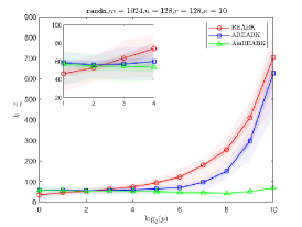
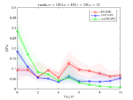
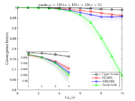
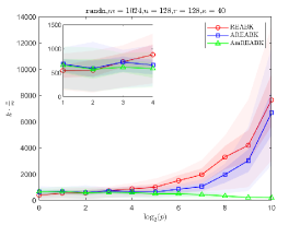
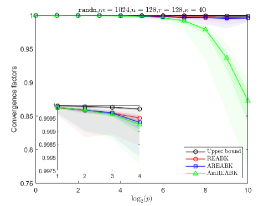
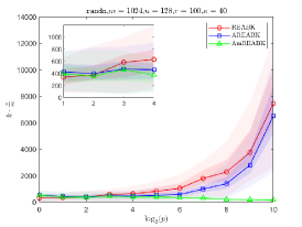
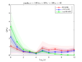
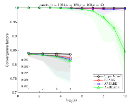
Figure 2. Figures illustrate the evolution of the number of full iterations (left), the CPU time (middle), and the actual convergence factor (right) with respect to the block size $p$. The title of each plot indicates the values of $m,n,r$, and $\kappa$. All computations are terminated once $\text{RSE}<10^{-12}$.

Table 1 and Figure 3 present the number of iterations and the computing time for REABK, AREABK, and AmREABK when applied to sparse matrices from SuiteSparse Matrix Collection and LIBSVM. The six matrices from SuiteSparse Matrix Collection are bibd_16_8, crew1, WorldCities, model1, ash958, and Franz1, and the three from LIBSVM are a9a, cod-rna, and ijcnn1, some of which are full rank while the others are rank-deficient.

Table 1 shows the numerical results on the matrices from SuiteSparse Matrix Collection. As displayed in Table 1, AmREABK is consistently better than AREABK in terms of iterations across all test cases. However, we note that AREABK may outperform AmREABK in terms of CPU time in specific cases, such as ash958 and Franz1. This is because AmREABK requires more computations at each step compared to REABK. Moreover, Table 1 also reveals that both AmREABK and AREABK outperform REABK in terms of both the number of iterations and CPU time for all test cases. Figure 3 presents the numerical results on the matrices from LIBSVM. Our results show that AmREABK still outperforms REABK and AREABK. Notably, for dataset cod-rna, it can be observed that only AmREABK successfully finds the solution, while both REABK and AREABK fail.

Table 1. The average Iter and CPU of REABK, AREABK, and AmREABK for linear systems with coefficient matrices from SuiteSparse Matrix Collection [26]. We set the block size $p=30$ and stop the algorithms once $\text{RSE}<10^{-12}$.

Matrix	$m\times n$	rank	$\frac{\sigma_{\max}(A)}{\sigma_{\min}(A)}$	REABK		AREABK		AmREABK
				Iter	CPU	Iter	CPU	Iter	CPU
bibd_16_8	$120\times 12870$	120	9.54	4082.62	2.3	2809.80	1.72	2150.14	1.61
crew1	$135\times 6469$	135	18.20	30092.90	5.51	3844.94	0.48	3380.62	0.45
WorldCities	$315\times 100$	100	6.60	70816.16	0.43	12551.30	0.08	3426.90	0.02
model1	$362\times 798$	362	17.57	84087.38	0.50	8153.02	0.051	6275.02	0.049
ash958	$958\times 292$	292	3.20	2931.34	0.029	991.16	0.0044	957.54	0.0054
Franz1	$2240\times 768$	755	2.74e+15	10040.46	0.31	3138.16	0.043	3063.08	0.068

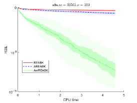
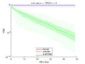
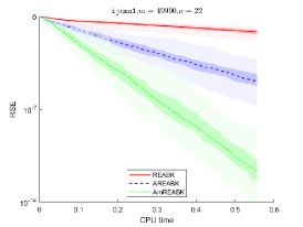
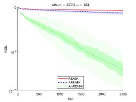
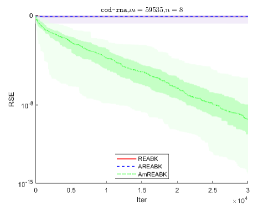
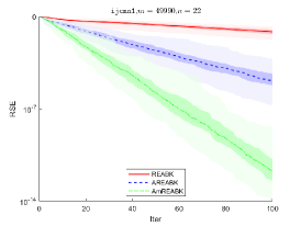
Figure 3. Performance of REABK, AREABK, and AmREABK for linear systems with coefficient matrices from LIBSVM [9]. Figures illustrate the evolution of RSE with respect to the number of iterations and the CPU time (in seconds). The title of each plot indicates the names and sizes of the data. We set the block size $p=300$ and stop the algorithms if the number of iterations exceeds a certain limit.

Next, we compare the performance of AmREABK with Matlab functions pinv and lsqminnorm. To obtain the minimum Euclidean norm least-squares solution easily, we use the randomly generated matrices with full column rank, where $m\geq n$ and $r=n$. This guarantees that $x^{*}$ is the desired unique minimum Euclidean norm least-squares solution.

During the test, AmREABK is implemented with different values of block size. We terminate AmREABK if the accuracy of its approximate solution is comparable to that of the approximate solution obtained by pinv and lsqminnorm. Figure 4 illustrates the CPU time against the number of rows with number of columns fixed. It can be observed that with an appropriate block size, AmREABK outperforms pinv and lsqminnorm, when the number of rows exceeds certain thresholds. Additionally, it is noteworthy that the performance of AmREABK is more sensitive to the increase in the condition number $\kappa$.

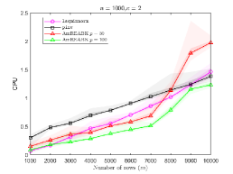
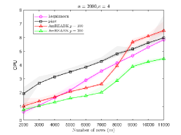
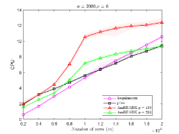
Figure 4. Figures illustrate the CPU time (in seconds) vs increasing number of rows. The title of each plot indicates the values of $n$ and $\kappa$.

6. Concluding remarks

We have developed a simple and versatile stochastic extended iterative algorithmic framework for finding the unique minimum norm least-squares solution for any linear system. Notably, we have incorporated the HBM technique into our algorithmic framework. We investigated to adaptively learn the parameters for the momentum variant of this method. Numerical results have confirmed the efficiency of our adaptive stochastic extended iterative method.

The randomized sparse Kaczmarz method proposed in [52] has been recognized as an effective strategy for obtaining sparse solutions to linear systems. A potential avenue for future research could be the extension of our adaptive stochastic extended iterative method to address sparse recovery problems, especially in situations where linear measurements are corrupted by noise. Additionally, Nesterov’s momentum [44, 43] has gained popularity as a momentum acceleration technique, and recent studies have introduced variants of Nesterov’s momentum for accelerating stochastic optimization algorithms [27]. Research on the incorporation of Nesterov’s momentum into our stochastic extended iterative method would also be a valuable topic.

7. Appendix. Proof of the main results

7.1. Proof of Theorem 3.4

Let us first introduce some notations. Define

(35) $$\overline{\mathcal{Q}}_{k}:=\{T_{k}\in\overline{\Omega}\mid T_{k}^{\top}A^{\top}z^{k}\neq 0\}\ \text{and}\ \mathcal{Q}_{k}:=\{S_{k}\in\Omega\mid S_{k}^{\top}(Ax^{k}-(b-z^{k+1}))\neq 0\}.$$

It is evident that $\{\overline{\mathcal{Q}}_{k},\overline{\mathcal{Q}}_{k}^{c}\}$ and $\{\mathcal{Q}_{k},\mathcal{Q}_{k}^{c}\}$ form partitions of $\overline{\Omega}$ and $\Omega$, respectively. We denote the conditional expectation based on the first $k$ iterations of Algorithm 1 as $\mathbb{E}_{k}[\cdot]$ i.e., $\mathbb{E}_{k}[\cdot]=\mathbb{E}\left[\cdot\mid T_{0},S_{0},T_{1},S_{1},\cdots,T_{k-1},S_{k-1}\right].$ Similarly, we denote the conditional expectation based on the first $k$ iterations and the sampling matrix $T_{k}$ as $\mathbb{E}_{S_{k}\in\Omega}[\cdot]$, i.e., $\mathbb{E}_{S_{k}\in\Omega}[\cdot]=\mathbb{E}\left[\cdot\mid T_{0},S_{0},T_{1},S_{1},\cdots,T_{k-1},S_{k-1},T_{k}\right].$ Then by the law of total expectation, we have

$$\mathbb{E}_{k}[\cdot]=\mathbb{E}_{k}\left[\mathbb{E}_{S_{k}\in\Omega}[\cdot]\right].$$

We have the following convergence result for the auxiliary sequence $\{z^{k}\}_{k\geq 0}$ generated by Algorithm 1.

Lemma 7.1.

Let $\{z^{k}\}_{k\geq 0}$ be the iteration sequence generated by Algorithm 1. Suppose that the probability space $(\overline{\Omega},\overline{\mathcal{F}},\overline{P})$ satisfies Assumption 2.1. Then

$$\mathbb{E}[\|z^{k}-b_{\text{Range}(A)^{\perp}}\|_{2}^{2}]\leq\rho_{z}^{k}\|z^{0}-b_{\text{Range}(A)^{\perp}}\|_{2}^{2},$$

where $\overline{H}$ and $\rho_{z}$ are defined as (21) and (22), respectively.

Proof.

Let $\overline{\mathcal{Q}}_{k}$ be defined as (35) and if the sampling matrix $T_{k}\in\overline{\mathcal{Q}}_{k}$, we have

$$\|z^{k+1}-b_{\text{Range}(A)^{\bot}}\|_{2}^{2}= \|z^{k}-\mu_{k}AT_{k}T_{k}^{\top}A^{\top}z^{k}-b_{\text{Range}(A)^{\bot}}\|_{2}^{2}$$

$$= \|z^{k}-b_{\text{Range}(A)^{\bot}}\|_{2}^{2}-2\mu_{k}\langle z^{k}-b_{\text{Range}(A)^{\bot}},AT_{k}T_{k}^{\top}A^{\top}z^{k}\rangle$$

$$+\mu_{k}^{2}\|AT_{k}T_{k}^{\top}A^{\top}z^{k}\|_{2}^{2}$$

$$= \|z^{k}-b_{\text{Range}(A)^{\bot}}\|_{2}^{2}-2(2-\eta)\overline{L}_{\text{adap}}^{(k)}\|T_{k}^{\top}A^{\top}z^{k}\|_{2}^{2}$$

$$+(2-\eta)^{2}\overline{L}_{\text{adap}}^{(k)}\|T_{k}^{\top}A^{\top}z^{k}\|_{2}^{2}$$

$$= \|z^{k}-b_{\text{Range}(A)^{\bot}}\|_{2}^{2}-\eta(2-\eta)\overline{L}_{\text{adap}}^{(k)}\|T_{k}^{\top}A^{\top}z^{k}\|_{2}^{2}$$

$$\leq \|z^{k}-b_{\text{Range}(A)^{\bot}}\|_{2}^{2}-\eta(2-\eta)\frac{\|T_{k}^{\top}A^{\top}z^{k}\|_{2}^{2}}{\|AT_{k}\|_{2}^{2}},$$

where the third equality follows from the definition of $\mu_{k}$ and $\overline{L}_{\text{adap}}^{(k)}$ in (16) and (17), respectively, and the last inequality follows from the fact that

$$\overline{L}_{\text{adap}}^{(k)}=\frac{\|T_{k}^{\top}A^{\top}z^{k}\|_{2}^{2}}{\|AT_{k}T_{k}^{\top}A^{\top}z^{k}\|_{2}^{2}}\geq\frac{1}{\|AT_{k}\|_{2}^{2}}.$$

Thus

$$\mathop{\mathbb{E}}\limits_{T_{k}\in\overline{\Omega}}[\|z^{k+1}-b_{\text{Range}(A)^{\bot}}\|_{2}^{2}]= \mathop{\mathbb{E}}\limits_{T_{k}\in\overline{\mathcal{Q}}_{k}}[\|z^{k+1}-b_{\text{Range}(A)^{\bot}}\|_{2}^{2}]+\mathop{\mathbb{E}}\limits_{T_{k}\in\overline{\mathcal{Q}}_{k}^{c}}[\|z^{k+1}-b_{\text{Range}(A)^{\bot}}\|_{2}^{2}]$$

$$\leq \mathop{\mathbb{E}}\limits_{T_{k}\in\overline{\mathcal{Q}}_{k}}\left[\|z^{k}-b_{\text{Range}(A)^{\bot}}\|_{2}^{2}-\eta(2-\eta)\frac{\|T_{k}^{\top}A^{\top}z^{k}\|_{2}^{2}}{\|AT_{k}\|_{2}^{2}}\right]$$

$$+\mathop{\mathbb{E}}\limits_{T_{k}\in\overline{\mathcal{Q}}_{k}^{c}}[\|z^{k}-b_{\text{Range}(A)^{\bot}}\|_{2}^{2}]$$

$$= \mathop{\mathbb{E}}\limits_{T_{k}\in\overline{\Omega}}[\|z^{k}-b_{\text{Range}(A)^{\bot}}\|_{2}^{2}]-\eta(2-\eta)\mathop{\mathbb{E}}\limits_{T_{k}\in\overline{\mathcal{Q}}_{k}}\left[\frac{\|T_{k}^{\top}A^{\top}z^{k}\|_{2}^{2}}{\|AT_{k}\|_{2}^{2}}\right]$$

$$= \|z^{k}-b_{\text{Range}(A)^{\bot}}\|_{2}^{2}-\eta(2-\eta)\mathop{\mathbb{E}}\limits_{T_{k}\in\overline{\Omega}}\left[\frac{\|T_{k}^{\top}A^{\top}z^{k}\|_{2}^{2}}{\|AT_{k}\|_{2}^{2}}\right]$$

$$= \|z^{k}-b_{\text{Range}(A)^{\bot}}\|_{2}^{2}-\eta(2-\eta)\|\overline{H}^{\frac{1}{2}}A^{\top}z^{k}\|_{2}^{2}$$

$$= \|z^{k}-b_{\text{Range}(A)^{\bot}}\|_{2}^{2}-\eta(2-\eta)\|\overline{H}^{\frac{1}{2}}A^{\top}(z^{k}-b_{\text{Range}(A)^{\bot}})\|_{2}^{2}$$

$$\leq \rho_{z}\|z^{k}-b_{\text{Range}(A)^{\perp}}\|_{2}^{2},$$

where the third equality follows from the fact that $\mathbb{E}_{T_{k}\in\overline{\mathcal{Q}}_{k}^{c}}\left[\frac{\|T_{k}^{\top}A^{\top}z^{k}\|_{2}^{2}}{\|AT_{k}\|_{2}^{2}}\right]=0$ as $T_{k}^{\top}A^{\top}z^{k}=0$ for $T_{k}\in\overline{\mathcal{Q}}_{k}^{c}$, and the last inequality follows from $\overline{H}$ is positive definite and $z^{k}-b_{\text{Range}(A)^{\perp}}\in\text{Range}(A)$. By taking the full expectation on both sides, we have

$$\mathbb{E}[\|z^{k}-b_{\text{Range}(A)^{\perp}}\|_{2}^{2}]\leq\rho_{z}^{k}\|z^{0}-b_{\text{Range}(A)^{\perp}}\|_{2}^{2}$$

as desired. ∎

Now, we are ready to prove Theorem 3.4.

Proof of Theorem 3.4.

Let $\mathcal{Q}_{k}$ be defined as (35) and if the sampling matrix $S_{k}\in\mathcal{Q}_{k}$, we have

(36) $$\|x^{k+1}-A^{\dagger}b\|_{2}^{2}= \|x^{k}-\alpha_{k}A^{\top}S_{k}S_{k}^{\top}(Ax^{k}-(b-z^{k+1}))-A^{\dagger}b\|_{2}^{2}$$

$$= \|x^{k}-A^{\dagger}b\|_{2}^{2}+\alpha_{k}^{2}\|A^{\top}S_{k}S_{k}^{\top}(Ax^{k}-(b-z^{k+1}))\|_{2}^{2}$$

$$-2\alpha_{k}\langle S_{k}^{\top}A(x^{k}-A^{\dagger}b),S_{k}^{\top}(Ax^{k}-(b-z^{k+1}))\rangle$$

$$= \|x^{k}-A^{\dagger}b\|_{2}^{2}+(2-\zeta)\alpha_{k}\|S_{k}^{\top}(Ax^{k}-(b-z^{k+1}))\|_{2}^{2}$$

$$-2\alpha_{k}\langle S_{k}^{\top}A(x^{k}-A^{\dagger}b),S_{k}^{\top}(Ax^{k}-(b-z^{k+1}))\rangle$$

$$= \|x^{k}-A^{\dagger}b\|_{2}^{2}+(2-\zeta)\alpha_{k}\|S_{k}^{\top}(Ax^{k}-(b-z^{k+1}))\|_{2}^{2}$$

$$+\alpha_{k}\left(\|S_{k}^{\top}(z^{k+1}-b_{\text{Range}(A)^{\bot}})\|_{2}^{2}-\|S_{k}^{\top}A(x^{k}-A^{\dagger}b)\|_{2}^{2}\right.$$

$$\left.\ \ \ \ \ \ \ \ \ \ \ -\|S_{k}^{\top}(Ax^{k}-(b-z^{k+1}))\|_{2}^{2}\right)$$

$$= \|x^{k}-A^{\dagger}b\|_{2}^{2}-\alpha_{k}\|S_{k}^{\top}A(x^{k}-A^{\dagger}b)\|_{2}^{2}+\alpha_{k}\|S_{k}^{\top}(z^{k+1}-b_{\text{Range}(A)^{\bot}})\|_{2}^{2}$$

$$-(\zeta-1)\alpha_{k}\|S_{k}^{\top}(Ax^{k}-(b-z^{k+1}))\|_{2}^{2},$$

where the third equality follows from the definition of $\alpha_{k}$ in (18). For any $0<\epsilon\leq 1$, we can get

(37) $$\|S_{k}^{\top}(Ax^{k}-(b-z^{k+1}))\|_{2}^{2}= \|S_{k}^{\top}(Ax^{k}-AA^{\dagger}b+AA^{\dagger}b-(b-z^{k+1}))\|_{2}^{2}$$

$$= \|S_{k}^{\top}A(x^{k}-A^{\dagger}b)+S_{k}^{\top}(z^{k+1}-b_{\text{Range}(A)^{\bot}})\|_{2}^{2}$$

$$\leq (1+\epsilon)\|S_{k}^{\top}A(x^{k}-A^{\dagger}b)\|_{2}^{2}+(\epsilon^{-1}+1)\|S_{k}^{\top}(z^{k+1}-b_{\text{Range}(A)^{\bot}})\|_{2}^{2},$$

and

(38) $$\|S_{k}^{\top}(Ax^{k}-(b-z^{k+1}))\|_{2}^{2}\geq(1-\epsilon)\|S_{k}^{\top}A(x^{k}-A^{\dagger}b)\|_{2}^{2}-(\epsilon^{-1}-1)\|S_{k}^{\top}(z^{k+1}-b_{\text{Range}(A)^{\bot}})\|_{2}^{2}.$$

For the case where $\zeta\in(0,1)$, substituting (37) into (36), we have

$$\|x^{k+1}-A^{\dagger}b\|_{2}^{2}\leq \|x^{k}-A^{\dagger}b\|_{2}^{2}-\left(1-(1+\epsilon)(1-\zeta)\right)\alpha_{k}\left\|S_{k}^{\top}A(x^{k}-A^{\dagger}b)\right\|_{2}^{2}$$

$$+\left(1+(\epsilon^{-1}+1)(1-\zeta)\right)\alpha_{k}\|S_{k}^{\top}(z^{k+1}-b_{\text{Range}(A)^{\bot}})\|_{2}^{2}$$

$$= \|x^{k}-A^{\dagger}b\|_{2}^{2}-c_{\zeta,\epsilon}L_{\text{adap}}^{(k)}\|S_{k}^{\top}A(x^{k}-A^{\dagger}b)\|_{2}^{2}$$

$$+d_{\zeta,\epsilon}L_{\text{adap}}^{(k)}\|S_{k}^{\top}(z^{k+1}-b_{\text{Range}(A)^{\bot}})\|_{2}^{2},$$

where $c_{\zeta,\epsilon}$ and $d_{\zeta,\epsilon}$ are given by (23) and (24), respectively. For the case where $\zeta\in[1,2)$, substituting (38) into (36), we have

$$\|x^{k+1}-A^{\dagger}b\|_{2}^{2}\leq \|x^{k}-A^{\dagger}b\|_{2}^{2}-\left(1+(1-\epsilon)(\zeta-1)\right)\alpha_{k}\|S_{k}^{\top}A(x^{k}-A^{\dagger}b)\|_{2}^{2}$$

$$+\left(1+(\epsilon^{-1}-1)(\zeta-1)\right)\alpha_{k}\|S_{k}^{\top}(z^{k+1}-b_{\text{Range}(A)^{\bot}})\|_{2}^{2}$$

$$= \|x^{k}-A^{\dagger}b\|_{2}^{2}-c_{\zeta,\epsilon}L_{\text{adap}}^{(k)}\|S_{k}^{\top}A(x^{k}-A^{\dagger}b)\|_{2}^{2}$$

$$+d_{\zeta,\epsilon}L_{\text{adap}}^{(k)}\|S_{k}^{\top}(z^{k+1}-b_{\text{Range}(A)^{\bot}})\|_{2}^{2}.$$

Thus, for any $\zeta\in(0,2)$, it holds that

(39) $$\mathop{\mathbb{E}}\limits_{S_{k}\in\Omega}[\|x^{k+1}-A^{\dagger}b\|_{2}^{2}]= \mathop{\mathbb{E}}\limits_{S_{k}\in\mathcal{Q}_{k}^{c}}[\|x^{k+1}-A^{\dagger}b\|_{2}^{2}]+\mathop{\mathbb{E}}\limits_{S_{k}\in\mathcal{Q}_{k}}[\|x^{k+1}-A^{\dagger}b\|_{2}^{2}]$$

$$\leq \mathop{\mathbb{E}}\limits_{S_{k}\in\mathcal{Q}_{k}^{c}}[\|x^{k}-A^{\dagger}b\|_{2}^{2}]+\mathop{\mathbb{E}}\limits_{S_{k}\in\mathcal{Q}_{k}}[\|x^{k}-A^{\dagger}b\|_{2}^{2}]$$

$$+\mathop{\mathbb{E}}\limits_{S_{k}\in\mathcal{Q}_{k}}\left[-c_{\zeta,\epsilon}L_{\text{adap}}^{(k)}\|S_{k}^{\top}A(x^{k}-A^{\dagger}b)\|_{2}^{2}\right.$$

$$\ \ \ \ \ \ \ \ \ \ \ \ \ \left.+d_{\zeta,\epsilon}L_{\text{adap}}^{(k)}\|S_{k}^{\top}(z^{k+1}-b_{\text{Range}(A)^{\bot}})\|_{2}^{2}\right]$$

$$= \|x^{k}-A^{\dagger}b\|_{2}^{2}-c_{\zeta,\epsilon}\underbrace{\mathop{\mathbb{E}}\limits_{S_{k}\in\mathcal{Q}_{k}}[L_{\text{adap}}^{(k)}\|S_{k}^{\top}A(x^{k}-A^{\dagger}b)\|_{2}^{2}]}_{ⓐ}$$

$$+d_{\zeta,\epsilon}\underbrace{\mathop{\mathbb{E}}\limits_{S_{k}\in\mathcal{Q}_{k}}[L_{\text{adap}}^{(k)}\|S_{k}^{\top}(z^{k+1}-b_{\text{Range}(A)^{\bot}})\|_{2}^{2}]}_{ⓑ}.$$

Next, we analyze the two expressions $ⓐ$ and $ⓑ$, respectively. Since

$$L_{\text{adap}}^{(k)}=\frac{\left\|S_{k}^{\top}\left(Ax^{k}-(b-z^{k+1})\right)\right\|_{2}^{2}}{\left\|A^{\top}S_{k}S_{k}^{\top}\left(Ax^{k}-(b-z^{k+1})\right)\right\|_{2}^{2}}\geq\frac{1}{\|A^{\top}S_{k}\|_{2}^{2}},$$

we can establish a lower bound for the first expression as

(40) $$ⓐ\geq \mathop{\mathbb{E}}\limits_{S_{k}\in\mathcal{Q}_{k}}\left[\frac{\left\|S_{k}^{\top}A(x^{k}-A^{\dagger}b)\right\|_{2}^{2}}{\|A^{\top}S_{k}\|_{2}^{2}}\right]=\mathop{\mathbb{E}}\limits_{S_{k}\in\Omega}\left[\frac{\left\|S_{k}^{\top}A(x^{k}-A^{\dagger}b)\right\|_{2}^{2}}{\|A^{\top}S_{k}\|_{2}^{2}}\right]-\mathop{\mathbb{E}}\limits_{S_{k}\in\mathcal{Q}_{k}^{c}}\left[\frac{\left\|S_{k}^{\top}A(x^{k}-A^{\dagger}b)\right\|_{2}^{2}}{\|A^{\top}S_{k}\|_{2}^{2}}\right]$$

$$\geq \sigma_{\min}^{2}(H^{\frac{1}{2}}A)\|x^{k}-A^{\dagger}b\|_{2}^{2}-\mathop{\mathbb{E}}\limits_{S_{k}\in\mathcal{Q}_{k}^{c}}\left[\frac{\left\|S_{k}^{\top}A(x^{k}-A^{\dagger}b)\right\|_{2}^{2}}{\|A^{\top}S_{k}\|_{2}^{2}}\right],$$

where the last inequality follows from $H=\mathop{\mathbb{E}}\limits_{S\in\Omega}\left[SS^{\top}/\left\|A^{\top}S\right\|_{2}^{2}\right]$ is positive definite and $x^{k}-A^{{\dagger}}b\in\text{Range}(A^{\top})$. Furthermore, note that if $S_{k}\in\mathcal{Q}_{k}^{c}$, i.e. $S_{k}^{\top}\left(Ax^{k}-(b-z^{k+1})\right)=0$, it holds that

$$S_{k}^{\top}A(x^{k}-A^{\dagger}b)= S_{k}^{\top}\left(Ax^{k}-(b-z^{k+1})+(b-z^{k+1})-AA^{\dagger}b\right)$$

$$= S_{k}^{\top}\left(Ax^{k}-(b-z^{k+1})\right)+S_{k}^{\top}(b_{\text{Range}(A)^{\bot}}-z^{k+1})$$

$$= S_{k}^{\top}(b_{\text{Range}(A)^{\bot}}-z^{k+1}).$$

Substituting it into (40), we can get

(41) $$ⓐ\geq \sigma_{\min}^{2}(H^{\frac{1}{2}}A)\|x^{k}-A^{\dagger}b\|_{2}^{2}-\mathop{\mathbb{E}}\limits_{S_{k}\in\mathcal{Q}_{k}^{c}}\left[\frac{\left\|S_{k}^{\top}(z^{k+1}-b_{\text{Range}(A)^{\bot}})\right\|_{2}^{2}}{\|A^{\top}S_{k}\|_{2}^{2}}\right].$$

In addition, since

$$L_{\text{adap}}^{(k)} =\frac{\left\|S_{k}^{\top}\left(Ax^{k}-(b-z^{k+1})\right)\right\|_{2}^{2}}{\left\|A^{\top}S_{k}S_{k}^{\top}\left(Ax^{k}-(b-z^{k+1})\right)\right\|_{2}^{2}}=\frac{\left\|S_{k}^{\top}A\left(x^{k}-A^{\dagger}(b-z^{k+1})\right)\right\|_{2}^{2}}{\left\|A^{\top}S_{k}S_{k}^{\top}A\left(x^{k}-A^{\dagger}(b-z^{k+1})\right)\right\|_{2}^{2}}$$

$$\leq\frac{1}{\lambda_{\min}\left(\frac{A^{\top}S_{k}S_{k}^{\top}A}{\|A^{\top}S_{k}\|_{2}^{2}}\right)\|A^{\top}S_{k}\|_{2}^{2}}\leq\frac{1}{\Lambda_{\min}\|A^{\top}S_{k}\|_{2}^{2}},$$

where the second equality follows from the fact that $b-z^{k+1}=AA^{\dagger}(b-z^{k+1})$ as $b-z^{k+1}\in\text{Range}(A)$. Hence, the second expression can be bounded as

(42) $$ⓑ\leq\frac{1}{\Lambda_{\min}}\mathop{\mathbb{E}}\limits_{S_{k}\in\mathcal{Q}_{k}}\left[\frac{\|S_{k}^{\top}(z^{k+1}-b_{\text{Range}(A)^{\bot}})\|_{2}^{2}}{\|A^{\top}S_{k}\|_{2}^{2}}\right].$$

By the assumptions of this theorem, specifically, if $\zeta\in(0,\frac{1}{2}]$ and $\epsilon\in(0,\frac{\zeta}{1-\zeta})$, or $\zeta\in(\frac{1}{2},2)$ and $\epsilon\in(0,1]$, it follows that $c_{\zeta,\epsilon}>0$. Furthermore, for any $\zeta\in(0,2)$ and $\epsilon\in(0,1]$, we have $d_{\zeta,\epsilon}>0$. Hence, by substituting (41) and (42) into (39), and noting that $\rho_{x}$ is defined as (25), we have

(43) $$\mathop{\mathbb{E}}\limits_{S_{k}\in\Omega}[\|x^{k+1}-A^{\dagger}b\|_{2}^{2}]\leq \rho_{x}\|x^{k}-A^{\dagger}b\|_{2}^{2}+c_{\zeta,\epsilon}\mathop{\mathbb{E}}\limits_{S_{k}\in\mathcal{Q}_{k}^{c}}\left[\frac{\|S_{k}^{\top}(z^{k+1}-b_{\text{Range}(A)^{\bot}})\|_{2}^{2}}{\|A^{\top}S_{k}\|_{2}^{2}}\right]$$

$$+ \frac{d_{\zeta,\epsilon}}{\Lambda_{\min}}\mathop{\mathbb{E}}\limits_{S_{k}\in\mathcal{Q}_{k}}\left[\frac{\|S_{k}^{\top}(z^{k+1}-b_{\text{Range}(A)^{\bot}})\|_{2}^{2}}{\|A^{\top}S_{k}\|_{2}^{2}}\right]$$

$$\leq \rho_{x}\|x^{k}-A^{\dagger}b\|_{2}^{2}+\frac{d_{\zeta,\epsilon}}{\Lambda_{\min}}\mathop{\mathbb{E}}\limits_{S_{k}\in\Omega}\left[\frac{\|S_{k}^{\top}(z^{k+1}-b_{\text{Range}(A)^{\bot}})\|_{2}^{2}}{\|A^{\top}S_{k}\|_{2}^{2}}\right]$$

$$\leq \rho_{x}\|x^{k}-A^{\dagger}b\|_{2}^{2}+\frac{d_{\zeta,\epsilon}\lambda_{\max}(H)}{\Lambda_{\min}}\|z^{k+1}-b_{\text{Range}(A)^{\bot}}\|_{2}^{2},$$

where the second inequality follows from the facts that $c_{\zeta,\epsilon}\leq d_{\zeta,\epsilon}$ and $\Lambda_{\min}\leq 1$. Thus,

$$\mathbb{E}_{k}\left[\|x^{k+1}-A^{\dagger}b\|_{2}^{2}\right]= \mathbb{E}_{k}\left[\mathbb{E}_{S_{k}\in\Omega}\left[\|x^{k+1}-A^{\dagger}b\|_{2}^{2}\right]\right]$$

$$\leq \rho_{x}\|x^{k}-A^{\dagger}b\|_{2}^{2}+\frac{d_{\zeta,\epsilon}\lambda_{\max}(H)}{\Lambda_{\min}}\mathbb{E}_{k}\left[\|z^{k+1}-b_{\text{Range}(A)^{\bot}}\|_{2}^{2}\right],$$

which together with Theorem 7.1 implies that

(44) $$\mathbb{E}\left[\|x^{k+1}-A^{\dagger}b\|_{2}^{2}\right]\leq \rho_{x}\mathbb{E}\left[\|x^{k}-A^{\dagger}b\|_{2}^{2}\right]+\frac{d_{\zeta,\epsilon}\lambda_{\max}(H)}{\Lambda_{\min}}\mathbb{E}\left[\|z^{k+1}-b_{\text{Range}(A)^{\bot}}\|_{2}^{2}\right]$$

$$\leq \rho_{x}\mathbb{E}\left[\|x^{k}-A^{\dagger}b\|_{2}^{2}\right]+\frac{d_{\zeta,\epsilon}\lambda_{\max}(H)\rho_{z}^{k+1}}{\Lambda_{\min}}\|z^{0}-b_{\text{Range}(A)^{\bot}}\|_{2}^{2}$$

$$\leq \rho_{x}^{2}\mathbb{E}\left[\|x^{k-1}-A^{\dagger}b\|_{2}^{2}\right]$$

$$+\frac{d_{\zeta,\epsilon}\lambda_{\max}(H)}{\Lambda_{\min}}\|z^{0}-b_{\text{Range}(A)^{\bot}}\|_{2}^{2}\left(\rho_{z}^{k}\rho_{x}+\rho_{z}^{k+1}\right)$$

$$\leq \rho_{x}^{k+1}\|x^{0}-A^{\dagger}b\|_{2}^{2}+\frac{d_{\zeta,\epsilon}\lambda_{\max}(H)}{\Lambda_{\min}}\|z^{0}-b_{\text{Range}(A)^{\bot}}\|_{2}^{2}\sum\limits_{i=0}^{k}\rho_{z}^{k+1-i}\rho_{x}^{i}.$$

For the case where $\rho_{x}\leq\rho_{z}$, we have

$$\sum\limits_{i=0}^{k}\rho_{z}^{k+1-i}\rho_{x}^{i}=\rho_{z}^{k+1}\sum\limits_{i=0}^{k}\left(\frac{\rho_{x}}{\rho_{z}}\right)^{i}\leq\frac{\rho_{z}^{k+1}}{\max\left\{1-\frac{\rho_{x}}{\rho_{z}},\frac{1}{k+1}\right\}}=\frac{\rho^{k+1}}{\max\left\{\left|1-\frac{\rho_{x}}{\rho_{z}}\right|,\frac{1}{k+1}\right\}},$$

where $\rho:=\max\{\rho_{x},\rho_{z}\}$. In addtion, for the case where $\rho_{z}<\rho_{x}$, we have

$$\sum\limits_{i=0}^{k}\rho_{z}^{k+1-i}\rho_{x}^{i}=\rho_{x}^{k+1}\sum\limits_{i=0}^{k}\left(\frac{\rho_{z}}{\rho_{x}}\right)^{k+1-i}\leq\frac{\rho_{x}^{k+1}}{\max\left\{\frac{\rho_{x}}{\rho_{z}}-1,\frac{1}{k+1}\right\}}\leq\frac{\rho^{k+1}}{\max\left\{\left|1-\frac{\rho_{x}}{\rho_{z}}\right|,\frac{1}{k+1}\right\}}.$$

Hence the inequality $\sum\limits_{i=0}^{k}\rho_{z}^{k+1-i}\rho_{x}^{i}\leq\frac{\rho^{k+1}}{\max\left\{\left|1-\frac{\rho_{x}}{\rho_{z}}\right|,\frac{1}{k+1}\right\}}$ holds for any $\rho_{z},\rho_{x}\in(0,1)$, which together with (44) implies that

$$\mathbb{E}\left[\|x^{k+1}-A^{\dagger}b\|_{2}^{2}\right]\leq \rho_{x}^{k+1}\|x^{0}-A^{\dagger}b\|_{2}^{2}+\frac{d_{\zeta,\epsilon}\lambda_{\max}(H)}{\Lambda_{\min}}\|z^{0}-b_{\text{Range}(A)^{\bot}}\|_{2}^{2}\sum\limits_{i=0}^{k}\rho_{z}^{k+1-i}\rho_{x}^{i}$$

$$\leq \rho^{k+1}\left(\|x^{0}-A^{\dagger}b\|_{2}^{2}+\frac{d_{\zeta,\epsilon}\lambda_{\max}(H)}{\Lambda_{\min}\max\left\{\left|1-\frac{\rho_{x}}{\rho_{z}}\right|,\frac{1}{k+1}\right\}}\|z^{0}-b_{\text{Range}(A)^{\bot}}\|_{2}^{2}\right).$$

This completes the proof of this theorem. ∎

7.2. Proof of Theorem 4.1

For convenience, we denote

$$\overline{z}^{k+1}=z^{k}-\overline{L}_{\text{adap}}^{(k)}AT_{k}T_{k}^{\top}A^{\top}z^{k},\quad\hat{x}^{k+1}=x^{k}-L_{\text{adap}}^{(k)}A^{\top}S_{k}S_{k}^{\top}(Ax^{k}-(b-z^{k+1})),$$

where $\overline{L}_{\text{adap}}^{(k)}$ and $L_{\text{adap}}^{(k)}$ is given by (17) and (19), respectively. We set

$$\overline{\mathcal{Q}}_{k,\neq}:=\{T_{k}\in\overline{\Omega}\mid\|p^{k}\|_{2}^{2}\|z^{k}-z^{k-1}\|_{2}^{2}-\langle p^{k},z^{k}-z^{k-1}\rangle^{2}\neq 0\},$$

and

$$\mathcal{Q}_{k,\neq}:=\{S_{k}\in\Omega\mid\|q^{k}\|_{2}^{2}\|x^{k}-x^{k-1}\|_{2}^{2}-\langle q^{k},x^{k}-x^{k-1}\rangle^{2}\neq 0\},$$

where $p^{k}:=AT_{k}T_{k}^{\top}A^{\top}z^{k}$ and $q^{k}:=A^{\top}S_{k}S_{k}^{\top}(Ax^{k}-(b-z^{k+1}))$.

Firstly, we can derive the following convergence result for the iteration sequence $\{z^{k}\}_{k\geq 0}$ generated by Algorithm 2.

Lemma 7.2.

Let $\{z^{k}\}_{k\geq 0}$ be the iteration sequence generated by Algorithm 2. Suppose that the probability space $(\overline{\Omega},\overline{\mathcal{F}},\overline{P})$ satisfies Assumption 2.1. Then

$$\mathbb{E}[\|z^{k}-b_{\text{Range}(A)^{\perp}}\|_{2}^{2}]\leq\left(1-\sigma_{\min}^{2}(\overline{H}^{\frac{1}{2}}A^{\top})\right)^{k}\|z^{0}-b_{\text{Range}(A)^{\perp}}\|_{2}^{2},$$

where $\overline{H}$ is defined as (21).

Proof of Lemma 7.2.

Since $\{\overline{\mathcal{Q}}_{k,\neq},\overline{\mathcal{Q}}_{k}\backslash\overline{\mathcal{Q}}_{k,\neq},\overline{\mathcal{Q}}_{k}^{c}\}$ forms a partition of $\overline{\Omega}$, hence the sampling matrix $T_{k}\in\overline{\Omega}$ can be classified into the following three cases: $T_{k}\in\overline{\mathcal{Q}}_{k,\neq}$, $T_{k}\in\overline{\mathcal{Q}}_{k}\backslash\overline{\mathcal{Q}}_{k,\neq}$, and $T_{k}\in\overline{\mathcal{Q}}_{k}^{c}$.

Case 1 $(T_{k}\in\overline{\mathcal{Q}}_{k,\neq})$: If the sampling matrix $T_{k}\in\overline{\mathcal{Q}}_{k,\neq}$, according to the definition of $z^{k+1}$, we have

$$\|z^{k+1}-b_{\text{Range}(A)^{\bot}}\|_{2}^{2}\leq\|\overline{z}^{k+1}-b_{\text{Range}(A)^{\bot}}\|_{2}^{2}.$$

Case 2 $(T_{k}\in\overline{\mathcal{Q}}_{k}\backslash\overline{\mathcal{Q}}_{k,\neq})$: If the sampling matrix $T_{k}\in\overline{\mathcal{Q}}_{k}\backslash\overline{\mathcal{Q}}_{k,\neq}$, we have $z^{k+1}=\overline{z}^{k+1}$.

Case 3 $(T_{k}\in\overline{\mathcal{Q}}_{k}^{c})$: If the sampling matrix $T_{k}\in\overline{\mathcal{Q}}_{k}^{c}$, we have $z^{k+1}=z^{k}$.

Therefore, it holds that

$$\mathop{\mathbb{E}}\limits_{T_{k}\in\overline{\Omega}}[\|z^{k+1}-b_{\text{Range}(A)^{\bot}}\|_{2}^{2}]\leq \mathop{\mathbb{E}}\limits_{T_{k}\in\overline{\mathcal{Q}}_{k,\neq}}[\|\overline{z}^{k+1}-b_{\text{Range}(A)^{\bot}}\|_{2}^{2}]$$

$$+\mathop{\mathbb{E}}\limits_{T_{k}\in\overline{\mathcal{Q}}_{k}\backslash\overline{\mathcal{Q}}_{k,\neq}}[\|\overline{z}^{k+1}-b_{\text{Range}(A)^{\bot}}\|_{2}^{2}]+\mathop{\mathbb{E}}\limits_{T_{k}\in\overline{\mathcal{Q}}_{k}^{c}}[\|z^{k}-b_{\text{Range}(A)^{\bot}}\|_{2}^{2}]$$

$$\leq \mathop{\mathbb{E}}\limits_{T_{k}\in\overline{\mathcal{Q}}_{k}}[\|\overline{z}^{k+1}-b_{\text{Range}(A)^{\bot}}\|_{2}^{2}]+\mathop{\mathbb{E}}\limits_{T_{k}\in\overline{\mathcal{Q}}_{k}^{c}}[\|z^{k}-b_{\text{Range}(A)^{\bot}}\|_{2}^{2}]$$

$$\leq \left(1-\sigma_{\min}^{2}(\overline{H}^{\frac{1}{2}}A^{\top})\right)\|z^{k}-b_{\text{Range}(A)^{\perp}}\|_{2}^{2},$$

where the last inequality from Lemma 7.1. By taking the full expectation on both sides, we have

$$\mathbb{E}[\|z^{k}-b_{\text{Range}(A)^{\perp}}\|_{2}^{2}]\leq\left(1-\sigma_{\min}^{2}(\overline{H}^{\frac{1}{2}}A^{\top})\right)^{k}\|z^{0}-b_{\text{Range}(A)^{\perp}}\|_{2}^{2}$$

as desired. ∎

Now we are ready to prove Theorem 4.1

Proof of Theorem 4.1.

Since $\{\mathcal{Q}_{k,\neq},\mathcal{Q}_{k}\backslash\mathcal{Q}_{k,\neq},\mathcal{Q}_{k}^{c}\}$ forms a partition of $\Omega$, the sampling matrix $S_{k}\in\Omega$ can be classified into the following three cases: $S_{k}\in\mathcal{Q}_{k,\neq}$, $S_{k}\in\mathcal{Q}_{k}\backslash\mathcal{Q}_{k,\neq}$, and $S_{k}\in\mathcal{Q}_{k}^{c}$.

Case 1 $(S_{k}\in\mathcal{Q}_{k,\neq})$: Let $\tilde{x}^{k+1}$ denote the orthogonal projection of $A^{\dagger}b$ onto the affine set $\Pi_{k}=x^{k}+\text{Span}\{q_{k},x^{k}-x^{k-1}\}$ and if the sampling matrix $S_{k}\in\mathcal{Q}_{k,\neq}$, we have $\langle\tilde{x}^{k+1}-A^{\dagger}b,\tilde{x}^{k+1}-x^{k+1}\rangle=0$. In addition, since $\hat{x}^{k+1}:=x^{k}-L_{\text{adap}}^{(k)}A^{\top}S_{k}S_{k}^{\top}(Ax^{k}-(b-z^{k+1}))\in\Pi_{k}$, we can get

(45) $$\|x^{k+1}-A^{\dagger}b\|_{2}^{2}= \|(x^{k+1}-\tilde{x}^{k+1})+(\tilde{x}^{k+1}-A^{\dagger}b)\|_{2}^{2}$$

$$= \|\tilde{x}^{k+1}-A^{\dagger}b\|_{2}^{2}+\|x^{k+1}-\tilde{x}^{k+1}\|_{2}^{2}$$

$$\leq \|\hat{x}^{k+1}-A^{\dagger}b\|_{2}^{2}+\|x^{k+1}-\tilde{x}^{k+1}\|_{2}^{2}.$$

According to the definitions of $x^{k+1}$ and $\tilde{x}^{k+1}$, it can be observed that the vector $x^{k+1}-\tilde{x}^{k+1}$ represents the orthogonal projection of the vector $A^{\dagger}(b-z^{k+1})-A^{\dagger}b=A^{\dagger}(b_{Range(A)^{\bot}}-z^{k+1})$ onto the affine set $\Pi_{k}$. Hence,

$$\|x^{k+1}-\tilde{x}^{k+1}\|_{2}^{2}\leq\|A^{\dagger}(z^{k+1}-b_{Range(A)^{\bot}})\|_{2}^{2}\leq\frac{\|z^{k+1}-b_{Range(A)^{\bot}}\|_{2}^{2}}{\sigma_{\min}^{2}(A)}.$$

Substituting it into (45), we can get

$$\|x^{k+1}-A^{\dagger}b\|_{2}^{2}\leq\|\hat{x}^{k+1}-A^{\dagger}b\|_{2}^{2}+\frac{\|z^{k+1}-b_{Range(A)^{\bot}}\|_{2}^{2}}{\sigma_{\min}^{2}(A)}.$$

Case 2 $(S_{k}\in\mathcal{Q}_{k}\backslash\mathcal{Q}_{k,\neq})$: If the sampling matrix $S_{k}\in\mathcal{Q}_{k}\backslash\mathcal{Q}_{k,\neq}$, it holds that $x^{k+1}=\hat{x}^{k+1}$.

Case 3 $(S_{k}\in\mathcal{Q}_{k}^{c})$: If the sampling matrix $S_{k}\in\mathcal{Q}_{k}^{c}$, it holds that $x^{k+1}=x^{k}$.

Recall $\hat{\rho}_{x}$ and $\gamma$ are defined as (33) and (34), respectively, we can obtain

$$\mathop{\mathbb{E}}\limits_{S_{k}\in\Omega_{k}}\left[\|x^{k+1}-A^{\dagger}b\|_{2}^{2}\right]$$

$$= \mathop{\mathbb{E}}\limits_{S_{k}\in\mathcal{Q}_{k,\neq}}\left[\|x^{k+1}-A^{\dagger}b\|_{2}^{2}\right]+\mathop{\mathbb{E}}\limits_{S_{k}\in\mathcal{Q}_{k}\backslash\mathcal{Q}_{k,\neq}}\left[\|x^{k+1}-A^{\dagger}b\|_{2}^{2}\right]+\mathop{\mathbb{E}}\limits_{S_{k}\in\mathcal{Q}_{k}^{c}}\left[\|x^{k+1}-A^{\dagger}b\|_{2}^{2}\right]$$

$$\leq \mathop{\mathbb{E}}\limits_{S_{k}\in\mathcal{Q}_{k}}\left[\|\hat{x}^{k+1}-A^{\dagger}b\|_{2}^{2}\right]+\mathop{\mathbb{E}}\limits_{S_{k}\in\mathcal{Q}_{k}^{c}}\left[\|x^{k}-A^{\dagger}b\|_{2}^{2}\right]+\frac{\|z^{k+1}-b_{Range(A)^{\bot}}\|_{2}^{2}}{\sigma_{\min}^{2}(A)}$$

$$\leq \hat{\rho}_{x}\|x^{k}-A^{\dagger}b\|_{2}^{2}+\frac{\lambda_{\max}(H)}{\Lambda_{\min}}\|z^{k+1}-b_{\text{Range}(A)^{\bot}}\|_{2}^{2}+\frac{\|z^{k+1}-b_{Range(A)^{\bot}}\|_{2}^{2}}{\sigma_{\min}^{2}(A)}$$

$$= \hat{\rho}_{x}\|x^{k}-A^{\dagger}b\|_{2}^{2}+\gamma\|z^{k+1}-b_{\text{Range}(A)^{\bot}}\|_{2}^{2},$$

where the second inequality follows from the definition of $\hat{x}^{k+1}$ and (43). Then, according to Lemma 7.2 and the proof of Theorem 3.4, define $\hat{\rho}:=\max\{\hat{\rho}_{z},\hat{\rho}_{x}\}$, we have

$$\mathbb{E}\left[\|x^{k+1}-A^{\dagger}b\|_{2}^{2}\right]\leq \hat{\rho}_{x}^{k+1}\|x^{0}-A^{\dagger}b\|_{2}^{2}+\gamma\|z^{0}-b_{\text{Range}(A)^{\bot}}\|_{2}^{2}\sum\limits_{i=0}^{k}\hat{\rho}_{z}^{k+1-i}\hat{\rho}_{x}^{i}$$

$$\leq \hat{\rho}^{k+1}\left(\|x^{0}-A^{\dagger}b\|_{2}^{2}+\frac{\gamma}{\max\left\{\left|1-\frac{\hat{\rho}_{x}}{\hat{\rho}_{z}}\right|,\frac{1}{k+1}\right\}}\|z^{0}-b_{\text{Range}(A)^{\bot}}\|_{2}^{2}\right).$$

This completes the proof of this theorem. ∎

References

• [1] Mario Arioli, Iain S Duff, and Peter PM de Rijk. On the augmented system approach to sparse least-squares problems. Numerische Mathematik, 55(6):667–684, 1989.
• [2] Zhong-Zhi Bai and Wen-Ting Wu. On greedy randomized Kaczmarz method for solving large sparse linear systems. SIAM J. Sci. Comput., 40(1):A592–A606, 2018.
• [3] Zhong-Zhi Bai and Wen-Ting Wu. On partially randomized extended Kaczmarz method for solving large sparse overdetermined inconsistent linear systems. Linear Algebra and Its Applications, 578:225–250, 2019.
• [4] Zhong-Zhi Bai and Wen-Ting Wu. On greedy randomized augmented Kaczmarz method for solving large sparse inconsistent linear systems. SIAM J. Sci. Comput., 43(6):A3892–A3911, 2021.
• [5] Mathieu Barré, Adrien Taylor, and Alexandre d’Aspremont. Complexity guarantees for Polyak steps with momentum. In Conference on Learning Theory, pages 452–478. PMLR, 2020.
• [6] Adi Ben-Israel and Thomas NE Greville. Generalized inverses: theory and applications, volume 15. Springer Science & Business Media, 2003.
• [7] Raghu Bollapragada, Tyler Chen, and Rachel Ward. On the fast convergence of minibatch heavy ball momentum. arXiv preprint arXiv:2206.07553, 2022.
• [8] Charles Byrne. A unified treatment of some iterative algorithms in signal processing and image reconstruction. Inverse Problems, 20(1):103–120, 2003.
• [9] Chih-Chung Chang and Chih-Jen Lin. LIBSVM: a library for support vector machines. ACM transactions on intelligent systems and technology (TIST), 2(3):1–27, 2011.
• [10] Kai-Wei Chang, Cho-Jui Hsieh, and Chih-Jen Lin. Coordinate descent method for large-scale l2-loss linear support vector machines. J. Mach. Learn. Res., 9(7):1369—1398, 2008.
• [11] Kui Du. Tight upper bounds for the convergence of the randomized extended Kaczmarz and Gauss-Seidel algorithms. Numer. Linear Algebra Appl., 26(3):e2233, 2019.
• [12] Kui Du, Wu-Tao Si, and Xiao-Hui Sun. Randomized extended average block Kaczmarz for solving least squares. SIAM J. Sci. Comput., 42(6):A3541–A3559, 2020.
• [13] Kui Du and Xiao-Hui Sun. Pseudoinverse-free randomized block iterative algorithms for consistent and inconsistent linear systems. arXiv preprint arXiv:2011.10353, 2020.
• [14] Ellen H Fukuda and Luis Mauricio Graña Drummond. A survey on multiobjective descent methods. Pesquisa Operacional, 34:585–620, 2014.
• [15] Euhanna Ghadimi, Hamid Reza Feyzmahdavian, and Mikael Johansson. Global convergence of the heavy-ball method for convex optimization. In 2015 European control conference (ECC), pages 310–315. IEEE, 2015.
• [16] Gene H Golub and Charles F Van Loan. Matrix computations. JHU press, 2013.
• [17] Richard Gordon, Robert Bender, and Gabor T Herman. Algebraic reconstruction techniques (ART) for three-dimensional electron microscopy and X-ray photography. J. Theor. Biol., 29(3):471–481, 1970.
• [18] Robert M Gower, Denali Molitor, Jacob Moorman, and Deanna Needell. On adaptive sketch-and-project for solving linear systems. SIAM J. Matrix Anal. Appl., 42(2):954–989, 2021.
• [19] Robert M. Gower and Peter Richtárik. Randomized iterative methods for linear systems. SIAM J. Matrix Anal. Appl., 36(4):1660–1690, 2015.
• [20] Deren Han, Yansheng Su, and Jiaxin Xie. Randomized Douglas-Rachford methods for linear systems: Improved accuracy and efficiency. SIAM J. Optim., 34(1):1045–1070, 2024.
• [21] Deren Han and Jiaxin Xie. On pseudoinverse-free randomized methods for linear systems: Unified framework and acceleration. arXiv preprint arXiv:2208.05437, 2022.
• [22] Martin Hanke and Wilhelm Niethammer. On the acceleration of Kaczmarz’s method for inconsistent linear systems. Linear Algebra and its Applications, 130:83–98, 1990.
• [23] Gabor T Herman and Lorraine B Meyer. Algebraic reconstruction techniques can be made computationally efficient (positron emission tomography application). IEEE Trans. Medical Imaging, 12(3):600–609, 1993.
• [24] Qinian Jin and Qin Huang. An adaptive heavy ball method for ill-posed inverse problems. arXiv preprint arXiv:2404.03218, 2024.
• [25] S Karczmarz. Angenäherte auflösung von systemen linearer glei-chungen. Bull. Int. Acad. Pol. Sic. Let., Cl. Sci. Math. Nat., pages 355–357, 1937.
• [26] Scott P Kolodziej, Mohsen Aznaveh, Matthew Bullock, Jarrett David, Timothy A Davis, Matthew Henderson, Yifan Hu, and Read Sandstrom. The suitesparse matrix collection website interface. J. Open Source Softw., 4(35):1244, 2019.
• [27] Guanghui Lan. First-order and stochastic optimization methods for machine learning. Springer, 2020.
• [28] Ji Liu and Stephen Wright. An accelerated randomized Kaczmarz algorithm. Math. Comp., 85(297):153–178, 2016.
• [29] Nicolas Loizou and Peter Richtárik. Momentum and stochastic momentum for stochastic gradient, newton, proximal point and subspace descent methods. Comput. Optim. Appl., 77(3):653–710, 2020.
• [30] Nicolas Loizou and Peter Richtárik. Revisiting randomized gossip algorithms: General framework, convergence rates and novel block and accelerated protocols. IEEE Trans. Inform. Theory, 67(12):8300–8324, 2021.
• [31] Dirk A Lorenz and Maximilian Winkler. Minimal error momentum Bregman-Kaczmarz. arXiv preprint arXiv:2307.15435, 2023.
• [32] Anna Ma and Deanna Needell. Stochastic gradient descent for linear systems with missing data. Numerical Mathematics: Theory, Methods and Applications, 12(1):1–20, 2019.
• [33] Anna Ma, Deanna Needell, and Aaditya Ramdas. Convergence properties of the randomized extended Gauss–Seidel and Kaczmarz methods. SIAM Journal on Matrix Analysis and Applications, 36(4):1590–1604, 2015.
• [34] Jacob D Moorman, Thomas K Tu, Denali Molitor, and Deanna Needell. Randomized Kaczmarz with averaging. BIT., 61(1):337–359, 2021.
• [35] Md Sarowar Morshed, Sabbir Ahmad, et al. Stochastic steepest descent methods for linear systems: Greedy sampling & momentum. arXiv preprint arXiv:2012.13087, 2020.
• [36] Frank Natterer. The mathematics of computerized tomography. SIAM, 2001.
• [37] I Necoara. Stochastic block projection algorithms with extrapolation for convex feasibility problems. Optimization Methods and Software, 37(5):1845–1875, 2022.
• [38] Ion Necoara. Faster randomized block Kaczmarz algorithms. SIAM J. Matrix Anal. Appl., 40(4):1425–1452, 2019.
• [39] Deanna Needell. Randomized Kaczmarz solver for noisy linear systems. BIT Numerical Mathematics, 50(2):395–403, 2010.
• [40] Deanna Needell, Nathan Srebro, and Rachel Ward. Stochastic gradient descent, weighted sampling, and the randomized Kaczmarz algorithm. Mathematical Programming, 155:549–573, 2016.
• [41] Deanna Needell and Joel A Tropp. Paved with good intentions: analysis of a randomized block Kaczmarz method. Linear Algebra and its Applications, 441:199–221, 2014.
• [42] Deanna Needell and Rachel Ward. Two-subspace projection method for coherent overdetermined systems. Journal of Fourier Analysis and Applications, 19(2):256–269, 2013.
• [43] Yurii Nesterov. Introductory lectures on convex optimization: A basic course, volume 87. Springer Science & Business Media, 2003.
• [44] Yurii E Nesterov. A method for solving the convex programming problem with convergence rate O$(1/k^{2})$. In Dokl. akad. nauk Sssr, volume 269, pages 543–547, 1983.
• [45] Boris T Polyak. Some methods of speeding up the convergence of iteration methods. Comput. Math. Math. Phys., 4(5):1–17, 1964.
• [46] Constantin Popa. Extensions of block-projections methods with relaxation parameters to inconsistent and rank-deficient least-squares problems. BIT Numerical Mathematics, 38(1):151–176, 1998.
• [47] Constantin Popa. Characterization of the solutions set of inconsistent least-squares problems by an extended Kaczmarz algorithm. Korean Journal of Computational and Applied Mathematics, 6(1):51–64, 1999.
• [48] Peter Richtárik and Martin Takácv. Stochastic reformulations of linear systems: Algorithms and convergence theory. SIAM J. Matrix Anal. Appl., 41(2):487–524, 2020.
• [49] Peter Richtárik and Martin Takáš. Stochastic reformulations of linear systems: algorithms and convergence theory. SIAM Journal on Matrix Analysis and Applications, 41(2):487–524, 2020.
• [50] Samer Saab Jr, Shashi Phoha, Minghui Zhu, and Asok Ray. An adaptive Polyak heavy-ball method. Machine Learning, 111(9):3245–3277, 2022.
• [51] Yoshikazu Sawaragi, Hirotaka Nakayama, and Tetsuzo Tanino. Theory of multiobjective optimization. Elsevier, 1985.
• [52] Frank Schöpfer and Dirk A Lorenz. Linear convergence of the randomized sparse Kaczmarz method. Math. Program., 173(1):509–536, 2019.
• [53] Othmane Sebbouh, Robert M Gower, and Aaron Defazio. Almost sure convergence rates for stochastic gradient descent and stochastic heavy ball. In Conference on Learning Theory, pages 3935–3971. PMLR, 2021.
• [54] Thomas Strohmer and Roman Vershynin. A randomized Kaczmarz algorithm with exponential convergence. J. Fourier Anal. Appl., 15(2):262–278, 2009.
• [55] Hiroki Tanabe, Ellen H Fukuda, and Nobuo Yamashita. Proximal gradient methods for multiobjective optimization and their applications. Computational Optimization and Applications, 72:339–361, 2019.
• [56] Nian-Ci Wu, Chengzhi Liu, Yatian Wang, and Qian Zuo. On the extended randomized multiple row method for solving linear least-squares problems. arXiv preprint arXiv:2210.03478, 2022.
• [57] Nian-Ci Wu and Hua Xiang. Semiconvergence analysis of the randomized row iterative method and its extended variants. Numerical Linear Algebra with Applications, 28(1):e2334, 2021.
• [58] Wen-Ting Wu. On two-subspace randomized extended Kaczmarz method for solving large linear least-squares problems. Numerical Algorithms, 89(1):1–31, 2022.
• [59] Yun Zeng, Deren Han, Yansheng Su, and Jiaxin Xie. Fast stochastic dual coordinate descent algorithms for linearly constrained convex optimization. arXiv preprint arXiv:2307.16702, 2023.
• [60] Yun Zeng, Deren Han, Yansheng Su, and Jiaxin Xie. On adaptive stochastic heavy ball momentum for solving linear systems. arXiv preprint arXiv:2305.05482, to appear in SIAM Journal on Matrix Analysis and Applications, 2023.
• [61] Yun Zeng, Deren Han, Yansheng Su, and Jiaxin Xie. Randomized kaczmarz method with adaptive stepsizes for inconsistent linear systems. Numerical Algorithms, 94(3):1403–1420, 2023.
• [62] Anastasios Zouzias and Nikolaos M. Freris. Randomized extended Kaczmarz for solving least squares. SIAM J. Matrix Anal. Appl., 34(2):773–793, 2013.