Finite-Choice Logic Programming

Robert J. Simmons robsimmons@gmail.com 0000-0003-2420-3067 UnaffiliatedUSA Michael Arntzenius 0009-0002-0417-5636 RelationalAIUnited Kingdom  and  Chris Martens c.martens@northeastern.edu 0000-0002-7026-0348 Northeastern University360 Huntington AveBostonMassachusettsUSA02115
Abstract.

Logic programming, as exemplified by datalog, defines the meaning of a program as the canonical smallest model derived from deductive closure over its inference rules. However, many problems call for an enumeration of models that vary along some set of choices while maintaining structural and logical constraints—there is no single canonical model. The notion of stable models has successfully captured programmer intuition about the set of valid solutions for such problems, giving rise to a family of programming languages and associated solvers collectively known as answer set programming. Unfortunately, the definition of a stable model is frustratingly indirect, especially in the presence of rules containing free variables.

We propose a new formalism, called finite-choice logic programming, for which the set of stable models can be characterized as the least fixed point of an immediate consequence operator. Our formalism allows straightforward expression of common idioms in both datalog and answer set programming, gives meaning to a new and useful class of programs, enjoys a constructive and direct operational semantics, and admits a predictive cost semantics, which we demonstrate through our implementation.

Datalog, answer set programming, bottom-up evaluation
copyright: noneconference: Make sure to enter the correct conference title from your rights confirmation email; May 28; 2024ccs: Computing methodologies Logic programming and answer set programmingccs: Theory of computation Constraint and logic programmingccs: Software and its engineering Constraint and logic languagesccs: Theory of computation Denotational semantics

1. Introduction

The generation of data according to structural and logical constraints is a problem seeing growing uptake and interest over the last decade, exemplified by applications like property-based random testing for typed functional programs (Goldstein et al., 2023; Goldstein and Pierce, 2022; Paraskevopoulou et al., 2022; Lampropoulos et al., 2017; Seidel et al., 2015; Claessen and Hughes, 2011), procedural content generation in games (Short and Adams, 2017; Shaker et al., 2016; Dormans and Bakkes, 2011), and reasoning about nondeterministic computation in distributed systems (Alvaro et al., 2011b). Answer set programming (ASP) (Gelfond and Lifschitz, 1988) is an approach to this task based on logic programming that has seen considerable, ongoing success in these and related domains (Smith and Mateas, 2011; Smith et al., 2013; Smith and Bryson, 2014; Neufeld et al., 2015; Summerville et al., 2018; Dabral and Martens, 2020; Dabral et al., 2023; Alvaro et al., 2011a), especially in contexts where there is a desire to combine functional constraints (e.g., well-typedness of a term, solvability of a puzzle, or consistency of a distributed program trace) with a diverse range of variability outside of those constraints.

To provide an expressive enough interface for programmers to represent problems of interest while retaining an intuitive semantics, ASP reconciles two incompatible intuitions about the meaning of logic programs. One intuition, exemplified by datalog, concerns positive information only: from a rule $p\leftarrow q_{1}\ldots q_{n}$, and a database containing $q_{1}\ldots q_{n}$, deduce $p$, where $p$ and $q_{i}$ are all positive assertions. The closure of deduction over such a program yields a single canonical model, the smallest set of assertions closed under the given implications; any other assertion is deemed false (Van Gelder et al., 1991).

The situation changes if we allow negative assertions such as p¬q𝑝𝑞{\color[rgb]{.5,.5,.5}\definecolor[named]{pgfstrokecolor}{rgb}{.5,.5,.5}\pgfsys@color@gray@stroke{.5}\pgfsys@color@gray@fill{.5}\mathit{p}}\leftarrow\neg{\color[rgb]{.5,.5,.5}\definecolor[named]{pgfstrokecolor}{rgb}{.5,.5,.5}\pgfsys@color@gray@stroke{.5}\pgfsys@color@gray@fill{.5}\mathit{q}}. We can preserve the deductive mindset by taking this rule to mean that if q𝑞{\color[rgb]{.5,.5,.5}\definecolor[named]{pgfstrokecolor}{rgb}{.5,.5,.5}\pgfsys@color@gray@stroke{.5}\pgfsys@color@gray@fill{.5}\mathit{q}} has no justification, then that suffices to justify p𝑝{\color[rgb]{.5,.5,.5}\definecolor[named]{pgfstrokecolor}{rgb}{.5,.5,.5}\pgfsys@color@gray@stroke{.5}\pgfsys@color@gray@fill{.5}\mathit{p}}. This program then has a single model that assigns p𝑝{\color[rgb]{.5,.5,.5}\definecolor[named]{pgfstrokecolor}{rgb}{.5,.5,.5}\pgfsys@color@gray@stroke{.5}\pgfsys@color@gray@fill{.5}\mathit{p}} to true and q𝑞{\color[rgb]{.5,.5,.5}\definecolor[named]{pgfstrokecolor}{rgb}{.5,.5,.5}\pgfsys@color@gray@stroke{.5}\pgfsys@color@gray@fill{.5}\mathit{q}} to false, as obviously q𝑞{\color[rgb]{.5,.5,.5}\definecolor[named]{pgfstrokecolor}{rgb}{.5,.5,.5}\pgfsys@color@gray@stroke{.5}\pgfsys@color@gray@fill{.5}\mathit{q}} has nothing to support its truth. Likewise, the canonical model of the logic program containing the single rule q¬p𝑞𝑝{\color[rgb]{.5,.5,.5}\definecolor[named]{pgfstrokecolor}{rgb}{.5,.5,.5}\pgfsys@color@gray@stroke{.5}\pgfsys@color@gray@fill{.5}\mathit{q}}\leftarrow\neg{\color[rgb]{.5,.5,.5}\definecolor[named]{pgfstrokecolor}{rgb}{.5,.5,.5}\pgfsys@color@gray@stroke{.5}\pgfsys@color@gray@fill{.5}\mathit{p}} assigns q𝑞{\color[rgb]{.5,.5,.5}\definecolor[named]{pgfstrokecolor}{rgb}{.5,.5,.5}\pgfsys@color@gray@stroke{.5}\pgfsys@color@gray@fill{.5}\mathit{q}} to true and p𝑝{\color[rgb]{.5,.5,.5}\definecolor[named]{pgfstrokecolor}{rgb}{.5,.5,.5}\pgfsys@color@gray@stroke{.5}\pgfsys@color@gray@fill{.5}\mathit{p}} to false. This intuition is cleanly captured by Przymusinski’s local stratification (Przymusinski, 1988). Local stratification is a condition sufficient to ensure the presence of a canonical model, and it is a satisfying distillation of the interpretation that if a proposition has no justification it is not true. This intuition remains a successful one, and is the foundation of almost all modern work on datalog and deductive databases.

What about the program containing the two rules p¬q𝑝𝑞{\color[rgb]{.5,.5,.5}\definecolor[named]{pgfstrokecolor}{rgb}{.5,.5,.5}\pgfsys@color@gray@stroke{.5}\pgfsys@color@gray@fill{.5}\mathit{p}}\leftarrow\neg{\color[rgb]{.5,.5,.5}\definecolor[named]{pgfstrokecolor}{rgb}{.5,.5,.5}\pgfsys@color@gray@stroke{.5}\pgfsys@color@gray@fill{.5}\mathit{q}} and q¬p𝑞𝑝{\color[rgb]{.5,.5,.5}\definecolor[named]{pgfstrokecolor}{rgb}{.5,.5,.5}\pgfsys@color@gray@stroke{.5}\pgfsys@color@gray@fill{.5}\mathit{q}}\leftarrow\neg{\color[rgb]{.5,.5,.5}\definecolor[named]{pgfstrokecolor}{rgb}{.5,.5,.5}\pgfsys@color@gray@stroke{.5}\pgfsys@color@gray@fill{.5}\mathit{p}}? There is no reasonable way for a canonical model to assign p𝑝{\color[rgb]{.5,.5,.5}\definecolor[named]{pgfstrokecolor}{rgb}{.5,.5,.5}\pgfsys@color@gray@stroke{.5}\pgfsys@color@gray@fill{.5}\mathit{p}} or q𝑞{\color[rgb]{.5,.5,.5}\definecolor[named]{pgfstrokecolor}{rgb}{.5,.5,.5}\pgfsys@color@gray@stroke{.5}\pgfsys@color@gray@fill{.5}\mathit{q}} to true or false, so it would seem that, following the deductive mindset, we must either reject this program outright or assign both p𝑝{\color[rgb]{.5,.5,.5}\definecolor[named]{pgfstrokecolor}{rgb}{.5,.5,.5}\pgfsys@color@gray@stroke{.5}\pgfsys@color@gray@fill{.5}\mathit{p}} and q𝑞{\color[rgb]{.5,.5,.5}\definecolor[named]{pgfstrokecolor}{rgb}{.5,.5,.5}\pgfsys@color@gray@stroke{.5}\pgfsys@color@gray@fill{.5}\mathit{q}} a third “indeterminate” value. But there’s a second intuition that says that we should forego canonicity and accept two different models: the one where p𝑝{\color[rgb]{.5,.5,.5}\definecolor[named]{pgfstrokecolor}{rgb}{.5,.5,.5}\pgfsys@color@gray@stroke{.5}\pgfsys@color@gray@fill{.5}\mathit{p}} is true and q𝑞{\color[rgb]{.5,.5,.5}\definecolor[named]{pgfstrokecolor}{rgb}{.5,.5,.5}\pgfsys@color@gray@stroke{.5}\pgfsys@color@gray@fill{.5}\mathit{q}} is false, and the one where p𝑝{\color[rgb]{.5,.5,.5}\definecolor[named]{pgfstrokecolor}{rgb}{.5,.5,.5}\pgfsys@color@gray@stroke{.5}\pgfsys@color@gray@fill{.5}\mathit{p}} is false and q𝑞{\color[rgb]{.5,.5,.5}\definecolor[named]{pgfstrokecolor}{rgb}{.5,.5,.5}\pgfsys@color@gray@stroke{.5}\pgfsys@color@gray@fill{.5}\mathit{q}} is true. One’s first impulse may be to fall back on the satisfiability of Boolean propositional formulas to explain this, but both these rules are classically equivalent to pq𝑝𝑞{\color[rgb]{.5,.5,.5}\definecolor[named]{pgfstrokecolor}{rgb}{.5,.5,.5}\pgfsys@color@gray@stroke{.5}\pgfsys@color@gray@fill{.5}\mathit{p}}\vee{\color[rgb]{.5,.5,.5}\definecolor[named]{pgfstrokecolor}{rgb}{.5,.5,.5}\pgfsys@color@gray@stroke{.5}\pgfsys@color@gray@fill{.5}\mathit{q}}, which has an additional model where p𝑝{\color[rgb]{.5,.5,.5}\definecolor[named]{pgfstrokecolor}{rgb}{.5,.5,.5}\pgfsys@color@gray@stroke{.5}\pgfsys@color@gray@fill{.5}\mathit{p}} and q𝑞{\color[rgb]{.5,.5,.5}\definecolor[named]{pgfstrokecolor}{rgb}{.5,.5,.5}\pgfsys@color@gray@stroke{.5}\pgfsys@color@gray@fill{.5}\mathit{q}} are both true. Clark addresses this issue by defining the completion of a program (Clark, 1978). The Clark completion of our little two rule program is represented by the formulas p¬q𝑝𝑞{\color[rgb]{.5,.5,.5}\definecolor[named]{pgfstrokecolor}{rgb}{.5,.5,.5}\pgfsys@color@gray@stroke{.5}\pgfsys@color@gray@fill{.5}\mathit{p}}\leftrightarrow\neg{\color[rgb]{.5,.5,.5}\definecolor[named]{pgfstrokecolor}{rgb}{.5,.5,.5}\pgfsys@color@gray@stroke{.5}\pgfsys@color@gray@fill{.5}\mathit{q}} and q¬p𝑞𝑝{\color[rgb]{.5,.5,.5}\definecolor[named]{pgfstrokecolor}{rgb}{.5,.5,.5}\pgfsys@color@gray@stroke{.5}\pgfsys@color@gray@fill{.5}\mathit{q}}\leftrightarrow\neg{\color[rgb]{.5,.5,.5}\definecolor[named]{pgfstrokecolor}{rgb}{.5,.5,.5}\pgfsys@color@gray@stroke{.5}\pgfsys@color@gray@fill{.5}\mathit{p}}. These formulas are classically equivalent to to (¬p¬q)(pq)𝑝𝑞𝑝𝑞(\neg{\color[rgb]{.5,.5,.5}\definecolor[named]{pgfstrokecolor}{rgb}{.5,.5,.5}\pgfsys@color@gray@stroke{.5}\pgfsys@color@gray@fill{.5}\mathit{p}}\vee\neg{\color[rgb]{.5,.5,.5}\definecolor[named]{pgfstrokecolor}{rgb}{.5,.5,.5}\pgfsys@color@gray@stroke{.5}\pgfsys@color@gray@fill{.5}\mathit{q}})\wedge({\color[rgb]{.5,.5,.5}\definecolor[named]{pgfstrokecolor}{rgb}{.5,.5,.5}\pgfsys@color@gray@stroke{.5}\pgfsys@color@gray@fill{.5}\mathit{p}}\vee{\color[rgb]{.5,.5,.5}\definecolor[named]{pgfstrokecolor}{rgb}{.5,.5,.5}\pgfsys@color@gray@stroke{.5}\pgfsys@color@gray@fill{.5}\mathit{q}}), which has precisely the two models we desire. The Clark completion is a satisfying distillation of the intuition that every true proposition must have some immediate justification.

Unfortunately, if we consider the program with two rules pq𝑝𝑞{\color[rgb]{.5,.5,.5}\definecolor[named]{pgfstrokecolor}{rgb}{.5,.5,.5}\pgfsys@color@gray@stroke{.5}\pgfsys@color@gray@fill{.5}\mathit{p}}\leftarrow{\color[rgb]{.5,.5,.5}\definecolor[named]{pgfstrokecolor}{rgb}{.5,.5,.5}\pgfsys@color@gray@stroke{.5}\pgfsys@color@gray@fill{.5}\mathit{q}} and qp𝑞𝑝{\color[rgb]{.5,.5,.5}\definecolor[named]{pgfstrokecolor}{rgb}{.5,.5,.5}\pgfsys@color@gray@stroke{.5}\pgfsys@color@gray@fill{.5}\mathit{q}}\leftarrow{\color[rgb]{.5,.5,.5}\definecolor[named]{pgfstrokecolor}{rgb}{.5,.5,.5}\pgfsys@color@gray@stroke{.5}\pgfsys@color@gray@fill{.5}\mathit{p}}, the Clark completion admits both the canonical model (where both p𝑝{\color[rgb]{.5,.5,.5}\definecolor[named]{pgfstrokecolor}{rgb}{.5,.5,.5}\pgfsys@color@gray@stroke{.5}\pgfsys@color@gray@fill{.5}\mathit{p}} and q𝑞{\color[rgb]{.5,.5,.5}\definecolor[named]{pgfstrokecolor}{rgb}{.5,.5,.5}\pgfsys@color@gray@stroke{.5}\pgfsys@color@gray@fill{.5}\mathit{q}} are false) and an additional model (where both p𝑝{\color[rgb]{.5,.5,.5}\definecolor[named]{pgfstrokecolor}{rgb}{.5,.5,.5}\pgfsys@color@gray@stroke{.5}\pgfsys@color@gray@fill{.5}\mathit{p}} and q𝑞{\color[rgb]{.5,.5,.5}\definecolor[named]{pgfstrokecolor}{rgb}{.5,.5,.5}\pgfsys@color@gray@stroke{.5}\pgfsys@color@gray@fill{.5}\mathit{q}} are true). As the intuition of logic programmers was formed in the context of deductive closure, the extra solution admitted by Clark’s completion feels like undesirably circular reasoning: the Clark completion is pq𝑝𝑞{\color[rgb]{.5,.5,.5}\definecolor[named]{pgfstrokecolor}{rgb}{.5,.5,.5}\pgfsys@color@gray@stroke{.5}\pgfsys@color@gray@fill{.5}\mathit{p}}\leftrightarrow{\color[rgb]{.5,.5,.5}\definecolor[named]{pgfstrokecolor}{rgb}{.5,.5,.5}\pgfsys@color@gray@stroke{.5}\pgfsys@color@gray@fill{.5}\mathit{q}}, and in the non-canonical model p𝑝{\color[rgb]{.5,.5,.5}\definecolor[named]{pgfstrokecolor}{rgb}{.5,.5,.5}\pgfsys@color@gray@stroke{.5}\pgfsys@color@gray@fill{.5}\mathit{p}} is justifying q𝑞{\color[rgb]{.5,.5,.5}\definecolor[named]{pgfstrokecolor}{rgb}{.5,.5,.5}\pgfsys@color@gray@stroke{.5}\pgfsys@color@gray@fill{.5}\mathit{q}} and vice versa.

Gelfond and Lifschitz’s notion of the stable models of an answer set program was successful at unifying these two intuitions. For locally stratified programs, answer set programming assigns a unique canonical model that matches the model suggested by local stratification. For programs without a canonical model, it combines the intuitions of Clark completion with a rejection of circular justification. Systems for computing the stable models of answer set programs have fruitfully co-evolved with the advancements in Boolean satisfiability solving, leading to sophisticated heuristics that make many problems fast in practice (Gebser et al., 2017) and resulting in mature tools (Gebser et al., 2011).

1.1. The compromise of stable models

Despite capturing programmer intuition so successfully, the actual semantic interpretation of an answer set program is quite indirect.

The first level of indirection is that the standard definition of stable models only applies to propositional logic programs without free variables. Consider this rule, which derives a fact when two nodes in a graph are not connected by an edge:

𝑛𝑜𝑡𝐶𝑜𝑛𝑛𝑒𝑐𝑡𝑒𝑑(x,y)𝑛𝑜𝑑𝑒(x),𝑛𝑜𝑑𝑒(y),¬𝑒𝑑𝑔𝑒(x,y)𝑛𝑜𝑡𝐶𝑜𝑛𝑛𝑒𝑐𝑡𝑒𝑑𝑥𝑦𝑛𝑜𝑑𝑒𝑥𝑛𝑜𝑑𝑒𝑦𝑒𝑑𝑔𝑒𝑥𝑦\displaystyle{{{\color[rgb]{.5,.5,.5}\definecolor[named]{pgfstrokecolor}{rgb}{.5,.5,.5}\pgfsys@color@gray@stroke{.5}\pgfsys@color@gray@fill{.5}\mathit{notConnected}}(x,y)}}\leftarrow{{{\color[rgb]{.5,.5,.5}\definecolor[named]{pgfstrokecolor}{rgb}{.5,.5,.5}\pgfsys@color@gray@stroke{.5}\pgfsys@color@gray@fill{.5}\mathit{node}}(x)}},{{{\color[rgb]{.5,.5,.5}\definecolor[named]{pgfstrokecolor}{rgb}{.5,.5,.5}\pgfsys@color@gray@stroke{.5}\pgfsys@color@gray@fill{.5}\mathit{node}}(y)}},\neg{{{\color[rgb]{.5,.5,.5}\definecolor[named]{pgfstrokecolor}{rgb}{.5,.5,.5}\pgfsys@color@gray@stroke{.5}\pgfsys@color@gray@fill{.5}\mathit{edge}}(x,y)}}

Answer set programming allows the illusion of rules containing free variables, but given base facts 𝑛𝑜𝑑𝑒(𝖺)𝑛𝑜𝑑𝑒𝖺{{{\color[rgb]{.5,.5,.5}\definecolor[named]{pgfstrokecolor}{rgb}{.5,.5,.5}\pgfsys@color@gray@stroke{.5}\pgfsys@color@gray@fill{.5}\mathit{node}}({\color[rgb]{0,.5,.5}\definecolor[named]{pgfstrokecolor}{rgb}{0,.5,.5}\mathsf{a}})}}, 𝑛𝑜𝑑𝑒(𝖻)𝑛𝑜𝑑𝑒𝖻{{{\color[rgb]{.5,.5,.5}\definecolor[named]{pgfstrokecolor}{rgb}{.5,.5,.5}\pgfsys@color@gray@stroke{.5}\pgfsys@color@gray@fill{.5}\mathit{node}}({\color[rgb]{0,.5,.5}\definecolor[named]{pgfstrokecolor}{rgb}{0,.5,.5}\mathsf{b}})}}, 𝑛𝑜𝑑𝑒(𝖼)𝑛𝑜𝑑𝑒𝖼{{{\color[rgb]{.5,.5,.5}\definecolor[named]{pgfstrokecolor}{rgb}{.5,.5,.5}\pgfsys@color@gray@stroke{.5}\pgfsys@color@gray@fill{.5}\mathit{node}}({\color[rgb]{0,.5,.5}\definecolor[named]{pgfstrokecolor}{rgb}{0,.5,.5}\mathsf{c}})}}, and 𝑒𝑑𝑔𝑒(𝖺,𝖻)𝑒𝑑𝑔𝑒𝖺𝖻{{{\color[rgb]{.5,.5,.5}\definecolor[named]{pgfstrokecolor}{rgb}{.5,.5,.5}\pgfsys@color@gray@stroke{.5}\pgfsys@color@gray@fill{.5}\mathit{edge}}({\color[rgb]{0,.5,.5}\definecolor[named]{pgfstrokecolor}{rgb}{0,.5,.5}\mathsf{a}},{\color[rgb]{0,.5,.5}\definecolor[named]{pgfstrokecolor}{rgb}{0,.5,.5}\mathsf{b}})}}, the stable models are only defined in terms of nine rules without free variables, one for each of the assignments of the free variables $x$ and $y$ to the variable-free terms ${\color[rgb]{0,.5,.5}\definecolor[named]{pgfstrokecolor}{rgb}{0,.5,.5}\mathsf{a}}$, ${\color[rgb]{0,.5,.5}\definecolor[named]{pgfstrokecolor}{rgb}{0,.5,.5}\mathsf{b}}$, and ${\color[rgb]{0,.5,.5}\definecolor[named]{pgfstrokecolor}{rgb}{0,.5,.5}\mathsf{c}}$. This is reflected in effectively all implementations of answer set programming, which involve the interaction of a solver that only understands variable-free rules and a grounder that generates variable-free rules, usually incorporating heuristics to minimize the number of rules that the the solver must deal with.

The second level of indirection is that even propositional answer set programs do not directly have a semantics. The definition of stable models for answer set programs first requires a syntactic transformation of an answer set program into a logic program without negation (the reduct, see Section 3.2 or (Gelfond and Lifschitz, 1988)). This transformation is defined with respect to a candidate model. If the unique model of the reduct is the same as the candidate model, the candidate model is accepted as an actual model. This fixed-point-like definition is what the “stability” of stable models refers to.

1.2. A constructive semantics based on mutually-exclusive choices

In this paper, we present finite-choice logic programming, an extension of forward-chaining logic programming that incorporates mutually-exclusive assignments of values to attributes. Facts take the form p(t¯)is¯v𝑝¯𝑡¯is𝑣{{{\color[rgb]{.5,.5,.5}\definecolor[named]{pgfstrokecolor}{rgb}{.5,.5,.5}\pgfsys@color@gray@stroke{.5}\pgfsys@color@gray@fill{.5}\mathit{p}}({\overline{t}})}\operatorname{{\color[rgb]{0,0,1}\definecolor[named]{pgfstrokecolor}{rgb}{0,0,1}{\underline{\textrm{{is}}}}}}{{v}}}, where p(t¯)𝑝¯𝑡{{{\color[rgb]{.5,.5,.5}\definecolor[named]{pgfstrokecolor}{rgb}{.5,.5,.5}\pgfsys@color@gray@stroke{.5}\pgfsys@color@gray@fill{.5}\mathit{p}}(\overline{t})}} is the attribute and $v$ is the unique value assigned to that attribute, and a set of facts (which we’ll call a database) must map each attribute to at most one value. Concretely, a fact like 𝑒𝑑𝑔𝑒𝐶𝑜𝑙𝑜𝑟(𝖺,𝖻)is¯𝖻𝗅𝗎𝖾𝑒𝑑𝑔𝑒𝐶𝑜𝑙𝑜𝑟𝖺𝖻¯is𝖻𝗅𝗎𝖾{{{\color[rgb]{.5,.5,.5}\definecolor[named]{pgfstrokecolor}{rgb}{.5,.5,.5}\pgfsys@color@gray@stroke{.5}\pgfsys@color@gray@fill{.5}\mathit{edgeColor}}({{\color[rgb]{0,.5,.5}\definecolor[named]{pgfstrokecolor}{rgb}{0,.5,.5}\mathsf{a}},{\color[rgb]{0,.5,.5}\definecolor[named]{pgfstrokecolor}{rgb}{0,.5,.5}\mathsf{b}}})}\operatorname{{\color[rgb]{0,0,1}\definecolor[named]{pgfstrokecolor}{rgb}{0,0,1}{\underline{\textrm{{is}}}}}}{{{\color[rgb]{0,.5,.5}\definecolor[named]{pgfstrokecolor}{rgb}{0,.5,.5}\mathsf{blue}}}}} would indicate that the edge from ${\color[rgb]{0,.5,.5}\definecolor[named]{pgfstrokecolor}{rgb}{0,.5,.5}\mathsf{a}}$ to ${\color[rgb]{0,.5,.5}\definecolor[named]{pgfstrokecolor}{rgb}{0,.5,.5}\mathsf{b}}$ is assigned the color blue, and cannot be any other color. This is called a functional dependency: a relation is a (partial) function if it maps an attribute to (at most) one value.

As we will see in Section 3, suitably choosing the domain of possible values allows us to treat finite-choice logic programming as a generalization of datalog without negation (if we restrict values to the single term ${\color[rgb]{0,.5,.5}\definecolor[named]{pgfstrokecolor}{rgb}{0,.5,.5}\mathsf{unit}}$) or as a generalization of answer set programming without a grounding step (if we restrict values to the two terms ${\color[rgb]{0,.5,.5}\definecolor[named]{pgfstrokecolor}{rgb}{0,.5,.5}\mathsf{tt}}$ and ${\color[rgb]{0,.5,.5}\definecolor[named]{pgfstrokecolor}{rgb}{0,.5,.5}\mathsf{ff}}$). But these are, fundamentally, the two most boring possible value domains! Finite-choice logic programming opens a much more expressive set of possibilities for logic programming.

Finite-choice logic programming specifies search problems through the interplay of two kinds of rules, which very loosely correspond to those two approaches:

  • A closed rule with the conclusion 𝑒𝑑𝑔𝑒𝐶𝑜𝑙𝑜𝑟(𝖺,𝖻)is¯{𝗀𝗋𝖾𝖾𝗇,𝗒𝖾𝗅𝗅𝗈𝗐}𝑒𝑑𝑔𝑒𝐶𝑜𝑙𝑜𝑟𝖺𝖻¯is𝗀𝗋𝖾𝖾𝗇𝗒𝖾𝗅𝗅𝗈𝗐{{{\color[rgb]{.5,.5,.5}\definecolor[named]{pgfstrokecolor}{rgb}{.5,.5,.5}\pgfsys@color@gray@stroke{.5}\pgfsys@color@gray@fill{.5}\mathit{edgeColor}}({{\color[rgb]{0,.5,.5}\definecolor[named]{pgfstrokecolor}{rgb}{0,.5,.5}\mathsf{a}},{\color[rgb]{0,.5,.5}\definecolor[named]{pgfstrokecolor}{rgb}{0,.5,.5}\mathsf{b}}})}\operatorname{{\color[rgb]{0,0,1}\definecolor[named]{pgfstrokecolor}{rgb}{0,0,1}{\underline{\textrm{{is}}}}}}{{\{{\color[rgb]{0,.5,.5}\definecolor[named]{pgfstrokecolor}{rgb}{0,.5,.5}\mathsf{green}},{\color[rgb]{0,.5,.5}\definecolor[named]{pgfstrokecolor}{rgb}{0,.5,.5}\mathsf{yellow}}\}}}} requires that the edge be either green or yellow if the rule’s premises are satisfied.

  • An open rule with the conclusion 𝑒𝑑𝑔𝑒𝐶𝑜𝑙𝑜𝑟(𝖺,𝖻)is?¯𝗋𝖾𝖽𝑒𝑑𝑔𝑒𝐶𝑜𝑙𝑜𝑟𝖺𝖻¯is?𝗋𝖾𝖽{{{\color[rgb]{.5,.5,.5}\definecolor[named]{pgfstrokecolor}{rgb}{.5,.5,.5}\pgfsys@color@gray@stroke{.5}\pgfsys@color@gray@fill{.5}\mathit{edgeColor}}({{\color[rgb]{0,.5,.5}\definecolor[named]{pgfstrokecolor}{rgb}{0,.5,.5}\mathsf{a}},{\color[rgb]{0,.5,.5}\definecolor[named]{pgfstrokecolor}{rgb}{0,.5,.5}\mathsf{b}}})}\operatorname{{\color[rgb]{0,0,1}\definecolor[named]{pgfstrokecolor}{rgb}{0,0,1}{\underline{\textrm{{is?}}}}}}{{{\color[rgb]{0,.5,.5}\definecolor[named]{pgfstrokecolor}{rgb}{0,.5,.5}\mathsf{red}}}}} permits the edge to be red if the premises apply. If the premises apply, the attribute 𝑒𝑑𝑔𝑒𝐶𝑜𝑙𝑜𝑟(𝖺,𝖻)𝑒𝑑𝑔𝑒𝐶𝑜𝑙𝑜𝑟𝖺𝖻{{{\color[rgb]{.5,.5,.5}\definecolor[named]{pgfstrokecolor}{rgb}{.5,.5,.5}\pgfsys@color@gray@stroke{.5}\pgfsys@color@gray@fill{.5}\mathit{edgeColor}}({\color[rgb]{0,.5,.5}\definecolor[named]{pgfstrokecolor}{rgb}{0,.5,.5}\mathsf{a}},{\color[rgb]{0,.5,.5}\definecolor[named]{pgfstrokecolor}{rgb}{0,.5,.5}\mathsf{b}})}} must take some value, but that value isn’t required to be ${\color[rgb]{0,.5,.5}\definecolor[named]{pgfstrokecolor}{rgb}{0,.5,.5}\mathsf{red}}$.

The interplay between open and closed rules is what allows finite-choice logic programming to subsume answer set programming. An answer set program containing the two rules p¬q𝑝𝑞{\color[rgb]{.5,.5,.5}\definecolor[named]{pgfstrokecolor}{rgb}{.5,.5,.5}\pgfsys@color@gray@stroke{.5}\pgfsys@color@gray@fill{.5}\mathit{p}}\leftarrow\neg{\color[rgb]{.5,.5,.5}\definecolor[named]{pgfstrokecolor}{rgb}{.5,.5,.5}\pgfsys@color@gray@stroke{.5}\pgfsys@color@gray@fill{.5}\mathit{q}} and q¬p𝑞𝑝{\color[rgb]{.5,.5,.5}\definecolor[named]{pgfstrokecolor}{rgb}{.5,.5,.5}\pgfsys@color@gray@stroke{.5}\pgfsys@color@gray@fill{.5}\mathit{q}}\leftarrow\neg{\color[rgb]{.5,.5,.5}\definecolor[named]{pgfstrokecolor}{rgb}{.5,.5,.5}\pgfsys@color@gray@stroke{.5}\pgfsys@color@gray@fill{.5}\mathit{p}} corresponds to the finite-choice logic program in Figure 1. The open rules 1 and 2 unconditionally permit p𝑝{\color[rgb]{.5,.5,.5}\definecolor[named]{pgfstrokecolor}{rgb}{.5,.5,.5}\pgfsys@color@gray@stroke{.5}\pgfsys@color@gray@fill{.5}\mathit{p}} or q𝑞{\color[rgb]{.5,.5,.5}\definecolor[named]{pgfstrokecolor}{rgb}{.5,.5,.5}\pgfsys@color@gray@stroke{.5}\pgfsys@color@gray@fill{.5}\mathit{q}} to have the “false” value ${\color[rgb]{0,.5,.5}\definecolor[named]{pgfstrokecolor}{rgb}{0,.5,.5}\mathsf{ff}}$, and the closed rules 3 and 4 ensure that the assignment of ${\color[rgb]{0,.5,.5}\definecolor[named]{pgfstrokecolor}{rgb}{0,.5,.5}\mathsf{ff}}$ to either p𝑝{\color[rgb]{.5,.5,.5}\definecolor[named]{pgfstrokecolor}{rgb}{.5,.5,.5}\pgfsys@color@gray@stroke{.5}\pgfsys@color@gray@fill{.5}\mathit{p}} or q𝑞{\color[rgb]{.5,.5,.5}\definecolor[named]{pgfstrokecolor}{rgb}{.5,.5,.5}\pgfsys@color@gray@stroke{.5}\pgfsys@color@gray@fill{.5}\mathit{q}} will force the other attribute to take the “true” value ${\color[rgb]{0,.5,.5}\definecolor[named]{pgfstrokecolor}{rgb}{0,.5,.5}\mathsf{tt}}$. The two solutions for this program are {pis¯𝗍𝗍,qis¯𝖿𝖿}𝑝¯is𝗍𝗍𝑞¯is𝖿𝖿\{{{{\color[rgb]{.5,.5,.5}\definecolor[named]{pgfstrokecolor}{rgb}{.5,.5,.5}\pgfsys@color@gray@stroke{.5}\pgfsys@color@gray@fill{.5}\mathit{p}}}\operatorname{{\color[rgb]{0,0,1}\definecolor[named]{pgfstrokecolor}{rgb}{0,0,1}{\underline{\textrm{{is}}}}}}{{{\color[rgb]{0,.5,.5}\definecolor[named]{pgfstrokecolor}{rgb}{0,.5,.5}\mathsf{tt}}}}},{{{\color[rgb]{.5,.5,.5}\definecolor[named]{pgfstrokecolor}{rgb}{.5,.5,.5}\pgfsys@color@gray@stroke{.5}\pgfsys@color@gray@fill{.5}\mathit{q}}}\operatorname{{\color[rgb]{0,0,1}\definecolor[named]{pgfstrokecolor}{rgb}{0,0,1}{\underline{\textrm{{is}}}}}}{{{\color[rgb]{0,.5,.5}\definecolor[named]{pgfstrokecolor}{rgb}{0,.5,.5}\mathsf{ff}}}}}\} and {pis¯𝖿𝖿,qis¯𝗍𝗍}𝑝¯is𝖿𝖿𝑞¯is𝗍𝗍\{{{{\color[rgb]{.5,.5,.5}\definecolor[named]{pgfstrokecolor}{rgb}{.5,.5,.5}\pgfsys@color@gray@stroke{.5}\pgfsys@color@gray@fill{.5}\mathit{p}}}\operatorname{{\color[rgb]{0,0,1}\definecolor[named]{pgfstrokecolor}{rgb}{0,0,1}{\underline{\textrm{{is}}}}}}{{{\color[rgb]{0,.5,.5}\definecolor[named]{pgfstrokecolor}{rgb}{0,.5,.5}\mathsf{ff}}}}},{{{\color[rgb]{.5,.5,.5}\definecolor[named]{pgfstrokecolor}{rgb}{.5,.5,.5}\pgfsys@color@gray@stroke{.5}\pgfsys@color@gray@fill{.5}\mathit{q}}}\operatorname{{\color[rgb]{0,0,1}\definecolor[named]{pgfstrokecolor}{rgb}{0,0,1}{\underline{\textrm{{is}}}}}}{{{\color[rgb]{0,.5,.5}\definecolor[named]{pgfstrokecolor}{rgb}{0,.5,.5}\mathsf{tt}}}}}\}, which correspond to the two solutions that answer set programming assigns to the source program.

(1) pis?¯𝖿𝖿𝑝¯is?𝖿𝖿\displaystyle{{{\color[rgb]{.5,.5,.5}\definecolor[named]{pgfstrokecolor}{rgb}{.5,.5,.5}\pgfsys@color@gray@stroke{.5}\pgfsys@color@gray@fill{.5}\mathit{p}}}\operatorname{{\color[rgb]{0,0,1}\definecolor[named]{pgfstrokecolor}{rgb}{0,0,1}{\underline{\textrm{{is?}}}}}}{{{\color[rgb]{0,.5,.5}\definecolor[named]{pgfstrokecolor}{rgb}{0,.5,.5}\mathsf{ff}}}}} $\displaystyle\leftarrow$
(2) qis?¯𝖿𝖿𝑞¯is?𝖿𝖿\displaystyle{{{\color[rgb]{.5,.5,.5}\definecolor[named]{pgfstrokecolor}{rgb}{.5,.5,.5}\pgfsys@color@gray@stroke{.5}\pgfsys@color@gray@fill{.5}\mathit{q}}}\operatorname{{\color[rgb]{0,0,1}\definecolor[named]{pgfstrokecolor}{rgb}{0,0,1}{\underline{\textrm{{is?}}}}}}{{{\color[rgb]{0,.5,.5}\definecolor[named]{pgfstrokecolor}{rgb}{0,.5,.5}\mathsf{ff}}}}} $\displaystyle\leftarrow$
(3) pis¯{𝗍𝗍}𝑝¯is𝗍𝗍\displaystyle{{{\color[rgb]{.5,.5,.5}\definecolor[named]{pgfstrokecolor}{rgb}{.5,.5,.5}\pgfsys@color@gray@stroke{.5}\pgfsys@color@gray@fill{.5}\mathit{p}}}\operatorname{{\color[rgb]{0,0,1}\definecolor[named]{pgfstrokecolor}{rgb}{0,0,1}{\underline{\textrm{{is}}}}}}{{\{{\color[rgb]{0,.5,.5}\definecolor[named]{pgfstrokecolor}{rgb}{0,.5,.5}\mathsf{tt}}\}}}} qis¯𝖿𝖿absent𝑞¯is𝖿𝖿\displaystyle\leftarrow{{{\color[rgb]{.5,.5,.5}\definecolor[named]{pgfstrokecolor}{rgb}{.5,.5,.5}\pgfsys@color@gray@stroke{.5}\pgfsys@color@gray@fill{.5}\mathit{q}}}\operatorname{{\color[rgb]{0,0,1}\definecolor[named]{pgfstrokecolor}{rgb}{0,0,1}{\underline{\textrm{{is}}}}}}{{{\color[rgb]{0,.5,.5}\definecolor[named]{pgfstrokecolor}{rgb}{0,.5,.5}\mathsf{ff}}}}}
(4) qis¯{𝗍𝗍}𝑞¯is𝗍𝗍\displaystyle{{{\color[rgb]{.5,.5,.5}\definecolor[named]{pgfstrokecolor}{rgb}{.5,.5,.5}\pgfsys@color@gray@stroke{.5}\pgfsys@color@gray@fill{.5}\mathit{q}}}\operatorname{{\color[rgb]{0,0,1}\definecolor[named]{pgfstrokecolor}{rgb}{0,0,1}{\underline{\textrm{{is}}}}}}{{\{{\color[rgb]{0,.5,.5}\definecolor[named]{pgfstrokecolor}{rgb}{0,.5,.5}\mathsf{tt}}\}}}} pis¯𝖿𝖿absent𝑝¯is𝖿𝖿\displaystyle\leftarrow{{{\color[rgb]{.5,.5,.5}\definecolor[named]{pgfstrokecolor}{rgb}{.5,.5,.5}\pgfsys@color@gray@stroke{.5}\pgfsys@color@gray@fill{.5}\mathit{p}}}\operatorname{{\color[rgb]{0,0,1}\definecolor[named]{pgfstrokecolor}{rgb}{0,0,1}{\underline{\textrm{{is}}}}}}{{{\color[rgb]{0,.5,.5}\definecolor[named]{pgfstrokecolor}{rgb}{0,.5,.5}\mathsf{ff}}}}}
Figure 1. The finite-choice logic program corresponding to the two rules p¬q𝑝𝑞{\color[rgb]{.5,.5,.5}\definecolor[named]{pgfstrokecolor}{rgb}{.5,.5,.5}\pgfsys@color@gray@stroke{.5}\pgfsys@color@gray@fill{.5}\mathit{p}}\leftarrow\neg{\color[rgb]{.5,.5,.5}\definecolor[named]{pgfstrokecolor}{rgb}{.5,.5,.5}\pgfsys@color@gray@stroke{.5}\pgfsys@color@gray@fill{.5}\mathit{q}} and q¬p𝑞𝑝{\color[rgb]{.5,.5,.5}\definecolor[named]{pgfstrokecolor}{rgb}{.5,.5,.5}\pgfsys@color@gray@stroke{.5}\pgfsys@color@gray@fill{.5}\mathit{q}}\leftarrow\neg{\color[rgb]{.5,.5,.5}\definecolor[named]{pgfstrokecolor}{rgb}{.5,.5,.5}\pgfsys@color@gray@stroke{.5}\pgfsys@color@gray@fill{.5}\mathit{p}} in ASP.

1.3. Contributions

The main contributions of this work include:

  • A straightforward definition of finite-choice logic programming that directly accounts for the incremental construction of programs with multiple solutions (Section 2).

  • A justification of answer set programming that doesn’t rely on rule grounding (Section 3, in particular Section 3.2).

  • A more involved definition of finite-choice logic programming that defines the meaning of a finite-choice logic program as the least fixed point of a monotonic immediate consequence operator that operates on sets of mutually exclusive models (Section 5).

  • A methodology for predicting the behavior of finite-choice logic programs based on the cost semantics for logic programs described by McAllester (McAllester, 2002) (Section 6.4).

  • The Dusa implementation of finite-choice logic programming (Section 6.6).

1.4. Related Work

Functional dependencies are not a new feature in logic programming. Systems like LogicBlox enforce invariants through functional dependencies, treating conflicts as errors that invalidate a transaction (Aref et al., 2015). A separate class of systems in the tradition of Krishnamurthy and Naqvi, including Soufflé, use relations with functional dependencies to allow a database to efficiently pick only one of a set of solutions (Krishnamurthy and Naqvi, 1988; Giannotti et al., 2001; Greco and Zaniolo, 2001; Hu et al., 2021). This is a very efficient approach when it is expressive enough, and we conjecture that Soufflé programs using their nondeterminstic choice operator can be faithfully translated into a finite-choice logic programs that only have open rules. Without an analogue of the closed rules in finite-choice logic programming, we believe these systems are unable to specify the search problems necessary to generalize answer set programming.

There have also been other approaches to constructively and incrementally generating stable models. Sacca and Zaniolo’s algorithm applied to general answer set programs, though it was primarily used to justify the nondeterminstic choice operation described above (Sacca and Zaniolo, 1990). We interpret their stable backtracking fixedpoint algorithm as potentially giving a direct implementation for answer set programming without grounding, though it seems to us that this significant fact was not noticed or exploited by the authors or anyone else. There has also been a disjunctive extension to datalog (Eiter et al., 1997) and characterizations of its stable models (Przymusinski, 1991), and Leone et al. (Leone et al., 1997) present an algorithm for incrementally deriving these stable models. Their approach is based on initially creating a single canonical model by letting some propositions be “partially true”. In these approaches to generating stable models, the set of solutions is presented only as the output of an algorithm, rather than denotationally. The choice sets we introduce in Section 5.3 are both foundational to our denotational semantics and to the implementation strategy we discuss in Section 6.

Our denotational semantics for finite-choice logic programming describes a domain-like structure for nondeterminism that draws inspiration from domain theory writ large (Scott, 1982), particularly powerdomains for nondeterministic lambda calculi and imperative programs (Plotkin, 1976; Smyth, 1976; Kennaway and Hoare, 1980). Our partial order relation on choice sets matches the one used for Smyth powerdomains in particular (Smyth, 1976). However, our construction requires certain completeness criteria on posets that differ from these and other domain definitions we have found in the literature.

2. The operational meaning of a finite-choice logic program

In this section, we define finite-choice logic programming with a nondeterministic operational semantics.

2.1. Programs

Definition 2.1 (Terms).

As common in logic programming settings, terms are Herbrand structures, either variables $x,y,z,\ldots$ or uninterpreted functions ${\color[rgb]{0,.5,.5}\definecolor[named]{pgfstrokecolor}{rgb}{0,.5,.5}\mathsf{f}}(t_{1},\ldots,t_{n})$ where the arguments $t_{i}$ are terms. Constants are functions with no arguments, and as usual we’ll leave the parentheses off and just write ${\color[rgb]{0,.5,.5}\definecolor[named]{pgfstrokecolor}{rgb}{0,.5,.5}\mathsf{b}}$ or ${\color[rgb]{0,.5,.5}\definecolor[named]{pgfstrokecolor}{rgb}{0,.5,.5}\mathsf{c}}$ instead of ${\color[rgb]{0,.5,.5}\definecolor[named]{pgfstrokecolor}{rgb}{0,.5,.5}\mathsf{b}}()$ or ${\color[rgb]{0,.5,.5}\definecolor[named]{pgfstrokecolor}{rgb}{0,.5,.5}\mathsf{c}}()$. We’ll often abbreviate sequences of terms $t_{1},\ldots,t_{n}$ as $\overline{t}$ when the indices aren’t important.

Definition 2.2 (Facts).

A fact has the form p(t1,,tn)is¯v𝑝subscript𝑡1subscript𝑡𝑛¯is𝑣{{{\color[rgb]{.5,.5,.5}\definecolor[named]{pgfstrokecolor}{rgb}{.5,.5,.5}\pgfsys@color@gray@stroke{.5}\pgfsys@color@gray@fill{.5}\mathit{p}}({t_{1},\ldots,t_{n}})}\operatorname{{\color[rgb]{0,0,1}\definecolor[named]{pgfstrokecolor}{rgb}{0,0,1}{\underline{\textrm{{is}}}}}}{{v}}}, where p𝑝{\color[rgb]{.5,.5,.5}\definecolor[named]{pgfstrokecolor}{rgb}{.5,.5,.5}\pgfsys@color@gray@stroke{.5}\pgfsys@color@gray@fill{.5}\mathit{p}} is a predicate and the $t_{i}$ and $v$ are variable-free (i.e. ground) terms. The first part, p(t1,,tn)𝑝subscript𝑡1subscript𝑡𝑛{{{\color[rgb]{.5,.5,.5}\definecolor[named]{pgfstrokecolor}{rgb}{.5,.5,.5}\pgfsys@color@gray@stroke{.5}\pgfsys@color@gray@fill{.5}\mathit{p}}(t_{1},\ldots,t_{n})}}, is the fact’s attribute, and $v$ is the fact’s value. We’ll sometimes use $a$ to stand in for variable-free attributes p(t¯)𝑝¯𝑡{{{\color[rgb]{.5,.5,.5}\definecolor[named]{pgfstrokecolor}{rgb}{.5,.5,.5}\pgfsys@color@gray@stroke{.5}\pgfsys@color@gray@fill{.5}\mathit{p}}(\overline{t})}}.

Definition 2.3 (Rules).

Rules $H\leftarrow R$ have one of two forms, open and closed.

(open form rule) p(t¯)is?¯v𝑝¯𝑡¯is?𝑣\displaystyle{{{\color[rgb]{.5,.5,.5}\definecolor[named]{pgfstrokecolor}{rgb}{.5,.5,.5}\pgfsys@color@gray@stroke{.5}\pgfsys@color@gray@fill{.5}\mathit{p}}({\overline{t}})}\operatorname{{\color[rgb]{0,0,1}\definecolor[named]{pgfstrokecolor}{rgb}{0,0,1}{\underline{\textrm{{is?}}}}}}{{v}}} $\displaystyle\leftarrow F$
(closed form rule, $m\geq 1$) p(t¯)is¯{v1,,vm}𝑝¯𝑡¯issubscript𝑣1subscript𝑣𝑚\displaystyle{{{\color[rgb]{.5,.5,.5}\definecolor[named]{pgfstrokecolor}{rgb}{.5,.5,.5}\pgfsys@color@gray@stroke{.5}\pgfsys@color@gray@fill{.5}\mathit{p}}({\overline{t}})}\operatorname{{\color[rgb]{0,0,1}\definecolor[named]{pgfstrokecolor}{rgb}{0,0,1}{\underline{\textrm{{is}}}}}}{{\{v_{1},\ldots,v_{m}\}}}} $\displaystyle\leftarrow F$

In both cases, the formula $F$ is a conjunction of premises of the form p(t¯)is¯v𝑝¯𝑡¯is𝑣{{{\color[rgb]{.5,.5,.5}\definecolor[named]{pgfstrokecolor}{rgb}{.5,.5,.5}\pgfsys@color@gray@stroke{.5}\pgfsys@color@gray@fill{.5}\mathit{p}}({\overline{t}})}\operatorname{{\color[rgb]{0,0,1}\definecolor[named]{pgfstrokecolor}{rgb}{0,0,1}{\underline{\textrm{{is}}}}}}{{v}}}, which may contain variables. The rule’s conclusion (or head) $H$ is the part to the left of the $\leftarrow$ symbol. Every variable appearing in the head $H$ must also appear in the formula $F$.

Definition 2.4 (Programs).

A program $P$ is a finite set of rules.

Definition 2.5 (Substitutions).

A substitution $\sigma$ is a total function from variables to ground terms. Applying a substitution to a term ($\sigma t$) or a formula ($\sigma F$) replaces all variables $x$ in the term or formula with the term $\sigma(x)$.

2.2. Operational semantics

Definition 2.6 (Database consistency).

A database $D$ is a set of facts. A database is consistent exactly when each attribute p(t¯)𝑝¯𝑡{{{\color[rgb]{.5,.5,.5}\definecolor[named]{pgfstrokecolor}{rgb}{.5,.5,.5}\pgfsys@color@gray@stroke{.5}\pgfsys@color@gray@fill{.5}\mathit{p}}(\overline{t})}} maps to at most one value $v$: if p(t¯)is¯vD𝑝¯𝑡¯is𝑣𝐷{{{\color[rgb]{.5,.5,.5}\definecolor[named]{pgfstrokecolor}{rgb}{.5,.5,.5}\pgfsys@color@gray@stroke{.5}\pgfsys@color@gray@fill{.5}\mathit{p}}({\overline{t}})}\operatorname{{\color[rgb]{0,0,1}\definecolor[named]{pgfstrokecolor}{rgb}{0,0,1}{\underline{\textrm{{is}}}}}}{{v}}}\in D and p(t¯)is¯vD𝑝¯𝑡¯issuperscript𝑣𝐷{{{\color[rgb]{.5,.5,.5}\definecolor[named]{pgfstrokecolor}{rgb}{.5,.5,.5}\pgfsys@color@gray@stroke{.5}\pgfsys@color@gray@fill{.5}\mathit{p}}({\overline{t}})}\operatorname{{\color[rgb]{0,0,1}\definecolor[named]{pgfstrokecolor}{rgb}{0,0,1}{\underline{\textrm{{is}}}}}}{{v^{\prime}}}}\in D, then $v=v^{\prime}$.

Definition 2.7 (Satisfaction).

We say that a substitution $\sigma$ satisfies $F$ in the database $D$ when, for each p(t¯)is¯v𝑝¯𝑡¯is𝑣{{{\color[rgb]{.5,.5,.5}\definecolor[named]{pgfstrokecolor}{rgb}{.5,.5,.5}\pgfsys@color@gray@stroke{.5}\pgfsys@color@gray@fill{.5}\mathit{p}}({\overline{t}})}\operatorname{{\color[rgb]{0,0,1}\definecolor[named]{pgfstrokecolor}{rgb}{0,0,1}{\underline{\textrm{{is}}}}}}{{v}}} in $F$, p(σt¯)is¯σv𝑝𝜎¯𝑡¯is𝜎𝑣{{{\color[rgb]{.5,.5,.5}\definecolor[named]{pgfstrokecolor}{rgb}{.5,.5,.5}\pgfsys@color@gray@stroke{.5}\pgfsys@color@gray@fill{.5}\mathit{p}}({\sigma\overline{t}})}\operatorname{{\color[rgb]{0,0,1}\definecolor[named]{pgfstrokecolor}{rgb}{0,0,1}{\underline{\textrm{{is}}}}}}{{\sigma v}}} is in $D$.

Definition 2.8 (Evolution).

The relation $D\operatorname{\Rightarrow}_{P}S$ relates a database to a set of databases:

  • If $P$ contains the closed-form rule p(t¯)is¯{v1,,vm}F𝑝¯𝑡¯issubscript𝑣1subscript𝑣𝑚𝐹{{{\color[rgb]{.5,.5,.5}\definecolor[named]{pgfstrokecolor}{rgb}{.5,.5,.5}\pgfsys@color@gray@stroke{.5}\pgfsys@color@gray@fill{.5}\mathit{p}}({\overline{t}})}\operatorname{{\color[rgb]{0,0,1}\definecolor[named]{pgfstrokecolor}{rgb}{0,0,1}{\underline{\textrm{{is}}}}}}{{\{v_{1},\ldots,v_{m}\}}}}\leftarrow F and $\sigma$ satisfies $F$ in $D$, then $D\operatorname{\Rightarrow}_{P}S$, where $S$ is the set of every consistent database D{p(σt¯)is¯σvi}𝐷𝑝𝜎¯𝑡¯is𝜎subscript𝑣𝑖D\cup\{{{{\color[rgb]{.5,.5,.5}\definecolor[named]{pgfstrokecolor}{rgb}{.5,.5,.5}\pgfsys@color@gray@stroke{.5}\pgfsys@color@gray@fill{.5}\mathit{p}}({\sigma\overline{t}})}\operatorname{{\color[rgb]{0,0,1}\definecolor[named]{pgfstrokecolor}{rgb}{0,0,1}{\underline{\textrm{{is}}}}}}{{\sigma v_{i}}}}\} for $1\leq i\leq m$.

  • If $P$ contains the open-form rule p(t1,,tn)is?¯vF𝑝subscript𝑡1subscript𝑡𝑛¯is?𝑣𝐹{{{\color[rgb]{.5,.5,.5}\definecolor[named]{pgfstrokecolor}{rgb}{.5,.5,.5}\pgfsys@color@gray@stroke{.5}\pgfsys@color@gray@fill{.5}\mathit{p}}({t_{1},\ldots,t_{n}})}\operatorname{{\color[rgb]{0,0,1}\definecolor[named]{pgfstrokecolor}{rgb}{0,0,1}{\underline{\textrm{{is?}}}}}}{{v}}}\leftarrow F and $\sigma$ satisfies $F$ in $D$, then $D\operatorname{\Rightarrow}_{P}S$, where $S$ contains one or two elements. $S$ always contains $D$ and, if the database D{p(σt¯)is¯σv}𝐷𝑝𝜎¯𝑡¯is𝜎𝑣D\cup\{{{{\color[rgb]{.5,.5,.5}\definecolor[named]{pgfstrokecolor}{rgb}{.5,.5,.5}\pgfsys@color@gray@stroke{.5}\pgfsys@color@gray@fill{.5}\mathit{p}}({\sigma\overline{t}})}\operatorname{{\color[rgb]{0,0,1}\definecolor[named]{pgfstrokecolor}{rgb}{0,0,1}{\underline{\textrm{{is}}}}}}{{\sigma v}}}\} is consistent, $S$ contains that database as well.

We say $D\operatorname{\leadsto}_{P}D^{\prime}$ if and only if $D\operatorname{\Rightarrow}_{P}S$ and $D^{\prime}\in S$. The relation $D\operatorname{\leadsto}^{*}_{P}D^{\prime}$ is the usual reflexive and transitive closure of $D\operatorname{\leadsto}_{P}D^{\prime}$.

Definition 2.9 (Saturation).

A database $D$ is saturated under a program $P$ if it can only evolve under the $\operatorname{\Rightarrow}_{P}$ relation to the singleton set containing itself. In other words, $D$ is saturated under $P$ if, for all $S$ such that $D\operatorname{\Rightarrow}_{P}S$, it is the case that $S=\{D\}$.

Definition 2.10 (Solutions).

A solution is a saturated database $D_{\textit{sol}}$ where $\varnothing\operatorname{\leadsto}^{*}_{P}D_{\textit{sol}}$. A solution for a consistent initial database $D_{\mathit{init}}$ is a saturated database $D_{\textit{sol}}$ where $D_{\mathit{init}}\operatorname{\leadsto}^{*}_{P}D_{\textit{sol}}$. Definition 2.8 ensures that $D_{\textit{sol}}$ must be consistent.

Definitions 2.9 and 2.10 are where we make critical use the fact that $\operatorname{\Rightarrow}_{P}$ is a relation between databases and sets of databases: we need to be able to identify rules that force conflicts onto the database. In a database D={pis¯𝖼}𝐷𝑝¯is𝖼D=\{{{{\color[rgb]{.5,.5,.5}\definecolor[named]{pgfstrokecolor}{rgb}{.5,.5,.5}\pgfsys@color@gray@stroke{.5}\pgfsys@color@gray@fill{.5}\mathit{p}}}\operatorname{{\color[rgb]{0,0,1}\definecolor[named]{pgfstrokecolor}{rgb}{0,0,1}{\underline{\textrm{{is}}}}}}{{{\color[rgb]{0,.5,.5}\definecolor[named]{pgfstrokecolor}{rgb}{0,.5,.5}\mathsf{c}}}}}\}, an applicable rule with the conclusion pis¯{𝖺}𝑝¯is𝖺{{{\color[rgb]{.5,.5,.5}\definecolor[named]{pgfstrokecolor}{rgb}{.5,.5,.5}\pgfsys@color@gray@stroke{.5}\pgfsys@color@gray@fill{.5}\mathit{p}}}\operatorname{{\color[rgb]{0,0,1}\definecolor[named]{pgfstrokecolor}{rgb}{0,0,1}{\underline{\textrm{{is}}}}}}{{\{{\color[rgb]{0,.5,.5}\definecolor[named]{pgfstrokecolor}{rgb}{0,.5,.5}\mathsf{a}}\}}}} means that $D\operatorname{\Rightarrow}_{P}\varnothing$, and therefore $D$ cannot be a solution.

2.3. Examples

Let $P$ be the four rule program from Figure 1 in Section 1.2. We demonstrate the operational semantics step-by-step, starting from the empty database $D_{0}=\varnothing$. Two rules apply, so there are two $S_{i}$ such that $\varnothing\operatorname{\Rightarrow}_{P}S_{i}$:

pis?¯𝖿𝖿𝑝¯is?𝖿𝖿\displaystyle{{{\color[rgb]{.5,.5,.5}\definecolor[named]{pgfstrokecolor}{rgb}{.5,.5,.5}\pgfsys@color@gray@stroke{.5}\pgfsys@color@gray@fill{.5}\mathit{p}}}\operatorname{{\color[rgb]{0,0,1}\definecolor[named]{pgfstrokecolor}{rgb}{0,0,1}{\underline{\textrm{{is?}}}}}}{{{\color[rgb]{0,.5,.5}\definecolor[named]{pgfstrokecolor}{rgb}{0,.5,.5}\mathsf{ff}}}}} $\displaystyle\leftarrow$ $\displaystyle\varnothing$ P{,{pis¯𝖿𝖿}}=S1subscript𝑃𝑝¯is𝖿𝖿subscript𝑆1\displaystyle\operatorname{\Rightarrow}_{P}\{\;\varnothing,\;\{{{{\color[rgb]{.5,.5,.5}\definecolor[named]{pgfstrokecolor}{rgb}{.5,.5,.5}\pgfsys@color@gray@stroke{.5}\pgfsys@color@gray@fill{.5}\mathit{p}}}\operatorname{{\color[rgb]{0,0,1}\definecolor[named]{pgfstrokecolor}{rgb}{0,0,1}{\underline{\textrm{{is}}}}}}{{{\color[rgb]{0,.5,.5}\definecolor[named]{pgfstrokecolor}{rgb}{0,.5,.5}\mathsf{ff}}}}}\}\;\}=S_{1}
qis?¯𝖿𝖿𝑞¯is?𝖿𝖿\displaystyle{{{\color[rgb]{.5,.5,.5}\definecolor[named]{pgfstrokecolor}{rgb}{.5,.5,.5}\pgfsys@color@gray@stroke{.5}\pgfsys@color@gray@fill{.5}\mathit{q}}}\operatorname{{\color[rgb]{0,0,1}\definecolor[named]{pgfstrokecolor}{rgb}{0,0,1}{\underline{\textrm{{is?}}}}}}{{{\color[rgb]{0,.5,.5}\definecolor[named]{pgfstrokecolor}{rgb}{0,.5,.5}\mathsf{ff}}}}} $\displaystyle\leftarrow$ $\displaystyle\varnothing$ P{,{qis¯𝖿𝖿}}=S2subscript𝑃𝑞¯is𝖿𝖿subscript𝑆2\displaystyle\operatorname{\Rightarrow}_{P}\{\;\varnothing,\;\{{{{\color[rgb]{.5,.5,.5}\definecolor[named]{pgfstrokecolor}{rgb}{.5,.5,.5}\pgfsys@color@gray@stroke{.5}\pgfsys@color@gray@fill{.5}\mathit{q}}}\operatorname{{\color[rgb]{0,0,1}\definecolor[named]{pgfstrokecolor}{rgb}{0,0,1}{\underline{\textrm{{is}}}}}}{{{\color[rgb]{0,.5,.5}\definecolor[named]{pgfstrokecolor}{rgb}{0,.5,.5}\mathsf{ff}}}}}\}\;\}=S_{2}
pis¯{𝗍𝗍}𝑝¯is𝗍𝗍\displaystyle{{{\color[rgb]{.5,.5,.5}\definecolor[named]{pgfstrokecolor}{rgb}{.5,.5,.5}\pgfsys@color@gray@stroke{.5}\pgfsys@color@gray@fill{.5}\mathit{p}}}\operatorname{{\color[rgb]{0,0,1}\definecolor[named]{pgfstrokecolor}{rgb}{0,0,1}{\underline{\textrm{{is}}}}}}{{\{{\color[rgb]{0,.5,.5}\definecolor[named]{pgfstrokecolor}{rgb}{0,.5,.5}\mathsf{tt}}\}}}} qis¯𝖿𝖿absent𝑞¯is𝖿𝖿\displaystyle\leftarrow{{{\color[rgb]{.5,.5,.5}\definecolor[named]{pgfstrokecolor}{rgb}{.5,.5,.5}\pgfsys@color@gray@stroke{.5}\pgfsys@color@gray@fill{.5}\mathit{q}}}\operatorname{{\color[rgb]{0,0,1}\definecolor[named]{pgfstrokecolor}{rgb}{0,0,1}{\underline{\textrm{{is}}}}}}{{{\color[rgb]{0,.5,.5}\definecolor[named]{pgfstrokecolor}{rgb}{0,.5,.5}\mathsf{ff}}}}} rule does not apply
qis¯{𝗍𝗍}𝑞¯is𝗍𝗍\displaystyle{{{\color[rgb]{.5,.5,.5}\definecolor[named]{pgfstrokecolor}{rgb}{.5,.5,.5}\pgfsys@color@gray@stroke{.5}\pgfsys@color@gray@fill{.5}\mathit{q}}}\operatorname{{\color[rgb]{0,0,1}\definecolor[named]{pgfstrokecolor}{rgb}{0,0,1}{\underline{\textrm{{is}}}}}}{{\{{\color[rgb]{0,.5,.5}\definecolor[named]{pgfstrokecolor}{rgb}{0,.5,.5}\mathsf{tt}}\}}}} pis¯𝖿𝖿absent𝑝¯is𝖿𝖿\displaystyle\leftarrow{{{\color[rgb]{.5,.5,.5}\definecolor[named]{pgfstrokecolor}{rgb}{.5,.5,.5}\pgfsys@color@gray@stroke{.5}\pgfsys@color@gray@fill{.5}\mathit{p}}}\operatorname{{\color[rgb]{0,0,1}\definecolor[named]{pgfstrokecolor}{rgb}{0,0,1}{\underline{\textrm{{is}}}}}}{{{\color[rgb]{0,.5,.5}\definecolor[named]{pgfstrokecolor}{rgb}{0,.5,.5}\mathsf{ff}}}}} rule does not apply
There are two possibilities for making progress. If we pick {pis¯𝖿𝖿}𝑝¯is𝖿𝖿\{{{{\color[rgb]{.5,.5,.5}\definecolor[named]{pgfstrokecolor}{rgb}{.5,.5,.5}\pgfsys@color@gray@stroke{.5}\pgfsys@color@gray@fill{.5}\mathit{p}}}\operatorname{{\color[rgb]{0,0,1}\definecolor[named]{pgfstrokecolor}{rgb}{0,0,1}{\underline{\textrm{{is}}}}}}{{{\color[rgb]{0,.5,.5}\definecolor[named]{pgfstrokecolor}{rgb}{0,.5,.5}\mathsf{ff}}}}}\} from $S_{1}$, three rules apply:
pis?¯𝖿𝖿𝑝¯is?𝖿𝖿\displaystyle{{{\color[rgb]{.5,.5,.5}\definecolor[named]{pgfstrokecolor}{rgb}{.5,.5,.5}\pgfsys@color@gray@stroke{.5}\pgfsys@color@gray@fill{.5}\mathit{p}}}\operatorname{{\color[rgb]{0,0,1}\definecolor[named]{pgfstrokecolor}{rgb}{0,0,1}{\underline{\textrm{{is?}}}}}}{{{\color[rgb]{0,.5,.5}\definecolor[named]{pgfstrokecolor}{rgb}{0,.5,.5}\mathsf{ff}}}}} $\displaystyle\leftarrow$ {pis¯𝖿𝖿}𝑝¯is𝖿𝖿\displaystyle\{{{{\color[rgb]{.5,.5,.5}\definecolor[named]{pgfstrokecolor}{rgb}{.5,.5,.5}\pgfsys@color@gray@stroke{.5}\pgfsys@color@gray@fill{.5}\mathit{p}}}\operatorname{{\color[rgb]{0,0,1}\definecolor[named]{pgfstrokecolor}{rgb}{0,0,1}{\underline{\textrm{{is}}}}}}{{{\color[rgb]{0,.5,.5}\definecolor[named]{pgfstrokecolor}{rgb}{0,.5,.5}\mathsf{ff}}}}}\} P{{pis¯𝖿𝖿}}=S3subscript𝑃𝑝¯is𝖿𝖿subscript𝑆3\displaystyle\operatorname{\Rightarrow}_{P}\{\;\{{{{\color[rgb]{.5,.5,.5}\definecolor[named]{pgfstrokecolor}{rgb}{.5,.5,.5}\pgfsys@color@gray@stroke{.5}\pgfsys@color@gray@fill{.5}\mathit{p}}}\operatorname{{\color[rgb]{0,0,1}\definecolor[named]{pgfstrokecolor}{rgb}{0,0,1}{\underline{\textrm{{is}}}}}}{{{\color[rgb]{0,.5,.5}\definecolor[named]{pgfstrokecolor}{rgb}{0,.5,.5}\mathsf{ff}}}}}\}\;\}=S_{3}
qis?¯𝖿𝖿𝑞¯is?𝖿𝖿\displaystyle{{{\color[rgb]{.5,.5,.5}\definecolor[named]{pgfstrokecolor}{rgb}{.5,.5,.5}\pgfsys@color@gray@stroke{.5}\pgfsys@color@gray@fill{.5}\mathit{q}}}\operatorname{{\color[rgb]{0,0,1}\definecolor[named]{pgfstrokecolor}{rgb}{0,0,1}{\underline{\textrm{{is?}}}}}}{{{\color[rgb]{0,.5,.5}\definecolor[named]{pgfstrokecolor}{rgb}{0,.5,.5}\mathsf{ff}}}}} $\displaystyle\leftarrow$ {pis¯𝖿𝖿}𝑝¯is𝖿𝖿\displaystyle\{{{{\color[rgb]{.5,.5,.5}\definecolor[named]{pgfstrokecolor}{rgb}{.5,.5,.5}\pgfsys@color@gray@stroke{.5}\pgfsys@color@gray@fill{.5}\mathit{p}}}\operatorname{{\color[rgb]{0,0,1}\definecolor[named]{pgfstrokecolor}{rgb}{0,0,1}{\underline{\textrm{{is}}}}}}{{{\color[rgb]{0,.5,.5}\definecolor[named]{pgfstrokecolor}{rgb}{0,.5,.5}\mathsf{ff}}}}}\} P{{pis¯𝖿𝖿},{pis¯𝖿𝖿,qis¯𝖿𝖿}}=S4subscript𝑃𝑝¯is𝖿𝖿𝑝¯is𝖿𝖿𝑞¯is𝖿𝖿subscript𝑆4\displaystyle\operatorname{\Rightarrow}_{P}\{\;\{{{{\color[rgb]{.5,.5,.5}\definecolor[named]{pgfstrokecolor}{rgb}{.5,.5,.5}\pgfsys@color@gray@stroke{.5}\pgfsys@color@gray@fill{.5}\mathit{p}}}\operatorname{{\color[rgb]{0,0,1}\definecolor[named]{pgfstrokecolor}{rgb}{0,0,1}{\underline{\textrm{{is}}}}}}{{{\color[rgb]{0,.5,.5}\definecolor[named]{pgfstrokecolor}{rgb}{0,.5,.5}\mathsf{ff}}}}}\},\;\{{{{\color[rgb]{.5,.5,.5}\definecolor[named]{pgfstrokecolor}{rgb}{.5,.5,.5}\pgfsys@color@gray@stroke{.5}\pgfsys@color@gray@fill{.5}\mathit{p}}}\operatorname{{\color[rgb]{0,0,1}\definecolor[named]{pgfstrokecolor}{rgb}{0,0,1}{\underline{\textrm{{is}}}}}}{{{\color[rgb]{0,.5,.5}\definecolor[named]{pgfstrokecolor}{rgb}{0,.5,.5}\mathsf{ff}}}}},{{{\color[rgb]{.5,.5,.5}\definecolor[named]{pgfstrokecolor}{rgb}{.5,.5,.5}\pgfsys@color@gray@stroke{.5}\pgfsys@color@gray@fill{.5}\mathit{q}}}\operatorname{{\color[rgb]{0,0,1}\definecolor[named]{pgfstrokecolor}{rgb}{0,0,1}{\underline{\textrm{{is}}}}}}{{{\color[rgb]{0,.5,.5}\definecolor[named]{pgfstrokecolor}{rgb}{0,.5,.5}\mathsf{ff}}}}}\}\;\}=S_{4}
pis¯{𝗍𝗍}𝑝¯is𝗍𝗍\displaystyle{{{\color[rgb]{.5,.5,.5}\definecolor[named]{pgfstrokecolor}{rgb}{.5,.5,.5}\pgfsys@color@gray@stroke{.5}\pgfsys@color@gray@fill{.5}\mathit{p}}}\operatorname{{\color[rgb]{0,0,1}\definecolor[named]{pgfstrokecolor}{rgb}{0,0,1}{\underline{\textrm{{is}}}}}}{{\{{\color[rgb]{0,.5,.5}\definecolor[named]{pgfstrokecolor}{rgb}{0,.5,.5}\mathsf{tt}}\}}}} qis¯𝖿𝖿absent𝑞¯is𝖿𝖿\displaystyle\leftarrow{{{\color[rgb]{.5,.5,.5}\definecolor[named]{pgfstrokecolor}{rgb}{.5,.5,.5}\pgfsys@color@gray@stroke{.5}\pgfsys@color@gray@fill{.5}\mathit{q}}}\operatorname{{\color[rgb]{0,0,1}\definecolor[named]{pgfstrokecolor}{rgb}{0,0,1}{\underline{\textrm{{is}}}}}}{{{\color[rgb]{0,.5,.5}\definecolor[named]{pgfstrokecolor}{rgb}{0,.5,.5}\mathsf{ff}}}}} rule does not apply
qis¯{𝗍𝗍}𝑞¯is𝗍𝗍\displaystyle{{{\color[rgb]{.5,.5,.5}\definecolor[named]{pgfstrokecolor}{rgb}{.5,.5,.5}\pgfsys@color@gray@stroke{.5}\pgfsys@color@gray@fill{.5}\mathit{q}}}\operatorname{{\color[rgb]{0,0,1}\definecolor[named]{pgfstrokecolor}{rgb}{0,0,1}{\underline{\textrm{{is}}}}}}{{\{{\color[rgb]{0,.5,.5}\definecolor[named]{pgfstrokecolor}{rgb}{0,.5,.5}\mathsf{tt}}\}}}} pis¯𝖿𝖿absent𝑝¯is𝖿𝖿\displaystyle\leftarrow{{{\color[rgb]{.5,.5,.5}\definecolor[named]{pgfstrokecolor}{rgb}{.5,.5,.5}\pgfsys@color@gray@stroke{.5}\pgfsys@color@gray@fill{.5}\mathit{p}}}\operatorname{{\color[rgb]{0,0,1}\definecolor[named]{pgfstrokecolor}{rgb}{0,0,1}{\underline{\textrm{{is}}}}}}{{{\color[rgb]{0,.5,.5}\definecolor[named]{pgfstrokecolor}{rgb}{0,.5,.5}\mathsf{ff}}}}} {pis¯𝖿𝖿}𝑝¯is𝖿𝖿\displaystyle\{{{{\color[rgb]{.5,.5,.5}\definecolor[named]{pgfstrokecolor}{rgb}{.5,.5,.5}\pgfsys@color@gray@stroke{.5}\pgfsys@color@gray@fill{.5}\mathit{p}}}\operatorname{{\color[rgb]{0,0,1}\definecolor[named]{pgfstrokecolor}{rgb}{0,0,1}{\underline{\textrm{{is}}}}}}{{{\color[rgb]{0,.5,.5}\definecolor[named]{pgfstrokecolor}{rgb}{0,.5,.5}\mathsf{ff}}}}}\} P{{pis¯𝖿𝖿,qis¯𝗍𝗍}}=S5subscript𝑃𝑝¯is𝖿𝖿𝑞¯is𝗍𝗍subscript𝑆5\displaystyle\operatorname{\Rightarrow}_{P}\{\;\{{{{\color[rgb]{.5,.5,.5}\definecolor[named]{pgfstrokecolor}{rgb}{.5,.5,.5}\pgfsys@color@gray@stroke{.5}\pgfsys@color@gray@fill{.5}\mathit{p}}}\operatorname{{\color[rgb]{0,0,1}\definecolor[named]{pgfstrokecolor}{rgb}{0,0,1}{\underline{\textrm{{is}}}}}}{{{\color[rgb]{0,.5,.5}\definecolor[named]{pgfstrokecolor}{rgb}{0,.5,.5}\mathsf{ff}}}}},{{{\color[rgb]{.5,.5,.5}\definecolor[named]{pgfstrokecolor}{rgb}{.5,.5,.5}\pgfsys@color@gray@stroke{.5}\pgfsys@color@gray@fill{.5}\mathit{q}}}\operatorname{{\color[rgb]{0,0,1}\definecolor[named]{pgfstrokecolor}{rgb}{0,0,1}{\underline{\textrm{{is}}}}}}{{{\color[rgb]{0,.5,.5}\definecolor[named]{pgfstrokecolor}{rgb}{0,.5,.5}\mathsf{tt}}}}}\}\;\}=S_{5}
Again, there are two databases we can pick to make progress. If we pick {pis¯𝖿𝖿,qis¯𝖿𝖿}𝑝¯is𝖿𝖿𝑞¯is𝖿𝖿\{{{{\color[rgb]{.5,.5,.5}\definecolor[named]{pgfstrokecolor}{rgb}{.5,.5,.5}\pgfsys@color@gray@stroke{.5}\pgfsys@color@gray@fill{.5}\mathit{p}}}\operatorname{{\color[rgb]{0,0,1}\definecolor[named]{pgfstrokecolor}{rgb}{0,0,1}{\underline{\textrm{{is}}}}}}{{{\color[rgb]{0,.5,.5}\definecolor[named]{pgfstrokecolor}{rgb}{0,.5,.5}\mathsf{ff}}}}},{{{\color[rgb]{.5,.5,.5}\definecolor[named]{pgfstrokecolor}{rgb}{.5,.5,.5}\pgfsys@color@gray@stroke{.5}\pgfsys@color@gray@fill{.5}\mathit{q}}}\operatorname{{\color[rgb]{0,0,1}\definecolor[named]{pgfstrokecolor}{rgb}{0,0,1}{\underline{\textrm{{is}}}}}}{{{\color[rgb]{0,.5,.5}\definecolor[named]{pgfstrokecolor}{rgb}{0,.5,.5}\mathsf{ff}}}}}\} from $S_{4}$, we will find ourselves in trouble.
pis?¯𝖿𝖿𝑝¯is?𝖿𝖿\displaystyle{{{\color[rgb]{.5,.5,.5}\definecolor[named]{pgfstrokecolor}{rgb}{.5,.5,.5}\pgfsys@color@gray@stroke{.5}\pgfsys@color@gray@fill{.5}\mathit{p}}}\operatorname{{\color[rgb]{0,0,1}\definecolor[named]{pgfstrokecolor}{rgb}{0,0,1}{\underline{\textrm{{is?}}}}}}{{{\color[rgb]{0,.5,.5}\definecolor[named]{pgfstrokecolor}{rgb}{0,.5,.5}\mathsf{ff}}}}} $\displaystyle\leftarrow$ {pis¯𝖿𝖿,qis¯𝖿𝖿}𝑝¯is𝖿𝖿𝑞¯is𝖿𝖿\displaystyle\{{{{\color[rgb]{.5,.5,.5}\definecolor[named]{pgfstrokecolor}{rgb}{.5,.5,.5}\pgfsys@color@gray@stroke{.5}\pgfsys@color@gray@fill{.5}\mathit{p}}}\operatorname{{\color[rgb]{0,0,1}\definecolor[named]{pgfstrokecolor}{rgb}{0,0,1}{\underline{\textrm{{is}}}}}}{{{\color[rgb]{0,.5,.5}\definecolor[named]{pgfstrokecolor}{rgb}{0,.5,.5}\mathsf{ff}}}}},{{{\color[rgb]{.5,.5,.5}\definecolor[named]{pgfstrokecolor}{rgb}{.5,.5,.5}\pgfsys@color@gray@stroke{.5}\pgfsys@color@gray@fill{.5}\mathit{q}}}\operatorname{{\color[rgb]{0,0,1}\definecolor[named]{pgfstrokecolor}{rgb}{0,0,1}{\underline{\textrm{{is}}}}}}{{{\color[rgb]{0,.5,.5}\definecolor[named]{pgfstrokecolor}{rgb}{0,.5,.5}\mathsf{ff}}}}}\} P{{pis¯𝖿𝖿,qis¯𝖿𝖿}}subscript𝑃𝑝¯is𝖿𝖿𝑞¯is𝖿𝖿\displaystyle\operatorname{\Rightarrow}_{P}\{\;\{{{{\color[rgb]{.5,.5,.5}\definecolor[named]{pgfstrokecolor}{rgb}{.5,.5,.5}\pgfsys@color@gray@stroke{.5}\pgfsys@color@gray@fill{.5}\mathit{p}}}\operatorname{{\color[rgb]{0,0,1}\definecolor[named]{pgfstrokecolor}{rgb}{0,0,1}{\underline{\textrm{{is}}}}}}{{{\color[rgb]{0,.5,.5}\definecolor[named]{pgfstrokecolor}{rgb}{0,.5,.5}\mathsf{ff}}}}},{{{\color[rgb]{.5,.5,.5}\definecolor[named]{pgfstrokecolor}{rgb}{.5,.5,.5}\pgfsys@color@gray@stroke{.5}\pgfsys@color@gray@fill{.5}\mathit{q}}}\operatorname{{\color[rgb]{0,0,1}\definecolor[named]{pgfstrokecolor}{rgb}{0,0,1}{\underline{\textrm{{is}}}}}}{{{\color[rgb]{0,.5,.5}\definecolor[named]{pgfstrokecolor}{rgb}{0,.5,.5}\mathsf{ff}}}}}\}\;\}
qis?¯𝖿𝖿𝑞¯is?𝖿𝖿\displaystyle{{{\color[rgb]{.5,.5,.5}\definecolor[named]{pgfstrokecolor}{rgb}{.5,.5,.5}\pgfsys@color@gray@stroke{.5}\pgfsys@color@gray@fill{.5}\mathit{q}}}\operatorname{{\color[rgb]{0,0,1}\definecolor[named]{pgfstrokecolor}{rgb}{0,0,1}{\underline{\textrm{{is?}}}}}}{{{\color[rgb]{0,.5,.5}\definecolor[named]{pgfstrokecolor}{rgb}{0,.5,.5}\mathsf{ff}}}}} $\displaystyle\leftarrow$ {pis¯𝖿𝖿,qis¯𝖿𝖿}𝑝¯is𝖿𝖿𝑞¯is𝖿𝖿\displaystyle\{{{{\color[rgb]{.5,.5,.5}\definecolor[named]{pgfstrokecolor}{rgb}{.5,.5,.5}\pgfsys@color@gray@stroke{.5}\pgfsys@color@gray@fill{.5}\mathit{p}}}\operatorname{{\color[rgb]{0,0,1}\definecolor[named]{pgfstrokecolor}{rgb}{0,0,1}{\underline{\textrm{{is}}}}}}{{{\color[rgb]{0,.5,.5}\definecolor[named]{pgfstrokecolor}{rgb}{0,.5,.5}\mathsf{ff}}}}},{{{\color[rgb]{.5,.5,.5}\definecolor[named]{pgfstrokecolor}{rgb}{.5,.5,.5}\pgfsys@color@gray@stroke{.5}\pgfsys@color@gray@fill{.5}\mathit{q}}}\operatorname{{\color[rgb]{0,0,1}\definecolor[named]{pgfstrokecolor}{rgb}{0,0,1}{\underline{\textrm{{is}}}}}}{{{\color[rgb]{0,.5,.5}\definecolor[named]{pgfstrokecolor}{rgb}{0,.5,.5}\mathsf{ff}}}}}\} P{{pis¯𝖿𝖿,qis¯𝖿𝖿}}subscript𝑃𝑝¯is𝖿𝖿𝑞¯is𝖿𝖿\displaystyle\operatorname{\Rightarrow}_{P}\{\;\{{{{\color[rgb]{.5,.5,.5}\definecolor[named]{pgfstrokecolor}{rgb}{.5,.5,.5}\pgfsys@color@gray@stroke{.5}\pgfsys@color@gray@fill{.5}\mathit{p}}}\operatorname{{\color[rgb]{0,0,1}\definecolor[named]{pgfstrokecolor}{rgb}{0,0,1}{\underline{\textrm{{is}}}}}}{{{\color[rgb]{0,.5,.5}\definecolor[named]{pgfstrokecolor}{rgb}{0,.5,.5}\mathsf{ff}}}}},{{{\color[rgb]{.5,.5,.5}\definecolor[named]{pgfstrokecolor}{rgb}{.5,.5,.5}\pgfsys@color@gray@stroke{.5}\pgfsys@color@gray@fill{.5}\mathit{q}}}\operatorname{{\color[rgb]{0,0,1}\definecolor[named]{pgfstrokecolor}{rgb}{0,0,1}{\underline{\textrm{{is}}}}}}{{{\color[rgb]{0,.5,.5}\definecolor[named]{pgfstrokecolor}{rgb}{0,.5,.5}\mathsf{ff}}}}}\}\;\}
pis¯{𝗍𝗍}𝑝¯is𝗍𝗍\displaystyle{{{\color[rgb]{.5,.5,.5}\definecolor[named]{pgfstrokecolor}{rgb}{.5,.5,.5}\pgfsys@color@gray@stroke{.5}\pgfsys@color@gray@fill{.5}\mathit{p}}}\operatorname{{\color[rgb]{0,0,1}\definecolor[named]{pgfstrokecolor}{rgb}{0,0,1}{\underline{\textrm{{is}}}}}}{{\{{\color[rgb]{0,.5,.5}\definecolor[named]{pgfstrokecolor}{rgb}{0,.5,.5}\mathsf{tt}}\}}}} qis¯𝖿𝖿absent𝑞¯is𝖿𝖿\displaystyle\leftarrow{{{\color[rgb]{.5,.5,.5}\definecolor[named]{pgfstrokecolor}{rgb}{.5,.5,.5}\pgfsys@color@gray@stroke{.5}\pgfsys@color@gray@fill{.5}\mathit{q}}}\operatorname{{\color[rgb]{0,0,1}\definecolor[named]{pgfstrokecolor}{rgb}{0,0,1}{\underline{\textrm{{is}}}}}}{{{\color[rgb]{0,.5,.5}\definecolor[named]{pgfstrokecolor}{rgb}{0,.5,.5}\mathsf{ff}}}}} rule does not apply
qis¯{𝗍𝗍}𝑞¯is𝗍𝗍\displaystyle{{{\color[rgb]{.5,.5,.5}\definecolor[named]{pgfstrokecolor}{rgb}{.5,.5,.5}\pgfsys@color@gray@stroke{.5}\pgfsys@color@gray@fill{.5}\mathit{q}}}\operatorname{{\color[rgb]{0,0,1}\definecolor[named]{pgfstrokecolor}{rgb}{0,0,1}{\underline{\textrm{{is}}}}}}{{\{{\color[rgb]{0,.5,.5}\definecolor[named]{pgfstrokecolor}{rgb}{0,.5,.5}\mathsf{tt}}\}}}} pis¯𝖿𝖿absent𝑝¯is𝖿𝖿\displaystyle\leftarrow{{{\color[rgb]{.5,.5,.5}\definecolor[named]{pgfstrokecolor}{rgb}{.5,.5,.5}\pgfsys@color@gray@stroke{.5}\pgfsys@color@gray@fill{.5}\mathit{p}}}\operatorname{{\color[rgb]{0,0,1}\definecolor[named]{pgfstrokecolor}{rgb}{0,0,1}{\underline{\textrm{{is}}}}}}{{{\color[rgb]{0,.5,.5}\definecolor[named]{pgfstrokecolor}{rgb}{0,.5,.5}\mathsf{ff}}}}} {pis¯𝖿𝖿,qis¯𝖿𝖿}𝑝¯is𝖿𝖿𝑞¯is𝖿𝖿\displaystyle\{{{{\color[rgb]{.5,.5,.5}\definecolor[named]{pgfstrokecolor}{rgb}{.5,.5,.5}\pgfsys@color@gray@stroke{.5}\pgfsys@color@gray@fill{.5}\mathit{p}}}\operatorname{{\color[rgb]{0,0,1}\definecolor[named]{pgfstrokecolor}{rgb}{0,0,1}{\underline{\textrm{{is}}}}}}{{{\color[rgb]{0,.5,.5}\definecolor[named]{pgfstrokecolor}{rgb}{0,.5,.5}\mathsf{ff}}}}},{{{\color[rgb]{.5,.5,.5}\definecolor[named]{pgfstrokecolor}{rgb}{.5,.5,.5}\pgfsys@color@gray@stroke{.5}\pgfsys@color@gray@fill{.5}\mathit{q}}}\operatorname{{\color[rgb]{0,0,1}\definecolor[named]{pgfstrokecolor}{rgb}{0,0,1}{\underline{\textrm{{is}}}}}}{{{\color[rgb]{0,.5,.5}\definecolor[named]{pgfstrokecolor}{rgb}{0,.5,.5}\mathsf{ff}}}}}\} $\displaystyle\operatorname{\Rightarrow}_{P}\varnothing$
The database {pis¯𝖿𝖿,qis¯𝖿𝖿}𝑝¯is𝖿𝖿𝑞¯is𝖿𝖿\{{{{\color[rgb]{.5,.5,.5}\definecolor[named]{pgfstrokecolor}{rgb}{.5,.5,.5}\pgfsys@color@gray@stroke{.5}\pgfsys@color@gray@fill{.5}\mathit{p}}}\operatorname{{\color[rgb]{0,0,1}\definecolor[named]{pgfstrokecolor}{rgb}{0,0,1}{\underline{\textrm{{is}}}}}}{{{\color[rgb]{0,.5,.5}\definecolor[named]{pgfstrokecolor}{rgb}{0,.5,.5}\mathsf{ff}}}}},{{{\color[rgb]{.5,.5,.5}\definecolor[named]{pgfstrokecolor}{rgb}{.5,.5,.5}\pgfsys@color@gray@stroke{.5}\pgfsys@color@gray@fill{.5}\mathit{q}}}\operatorname{{\color[rgb]{0,0,1}\definecolor[named]{pgfstrokecolor}{rgb}{0,0,1}{\underline{\textrm{{is}}}}}}{{{\color[rgb]{0,.5,.5}\definecolor[named]{pgfstrokecolor}{rgb}{0,.5,.5}\mathsf{ff}}}}}\} is not saturated, because although there exist transitions to the singleton set containing itself, our definition of saturation requires all possible transitions to yield the singleton set containing itself. In particular, rule 4 requires the program to derive qis¯𝗍𝗍𝑞¯is𝗍𝗍{{{\color[rgb]{.5,.5,.5}\definecolor[named]{pgfstrokecolor}{rgb}{.5,.5,.5}\pgfsys@color@gray@stroke{.5}\pgfsys@color@gray@fill{.5}\mathit{q}}}\operatorname{{\color[rgb]{0,0,1}\definecolor[named]{pgfstrokecolor}{rgb}{0,0,1}{\underline{\textrm{{is}}}}}}{{{\color[rgb]{0,.5,.5}\definecolor[named]{pgfstrokecolor}{rgb}{0,.5,.5}\mathsf{tt}}}}}, which conflicts with the existing fact qis¯𝖿𝖿𝑞¯is𝖿𝖿{{{\color[rgb]{.5,.5,.5}\definecolor[named]{pgfstrokecolor}{rgb}{.5,.5,.5}\pgfsys@color@gray@stroke{.5}\pgfsys@color@gray@fill{.5}\mathit{q}}}\operatorname{{\color[rgb]{0,0,1}\definecolor[named]{pgfstrokecolor}{rgb}{0,0,1}{\underline{\textrm{{is}}}}}}{{{\color[rgb]{0,.5,.5}\definecolor[named]{pgfstrokecolor}{rgb}{0,.5,.5}\mathsf{ff}}}}}. If instead choose {pis¯𝖿𝖿,qis¯𝗍𝗍}𝑝¯is𝖿𝖿𝑞¯is𝗍𝗍\{{{{\color[rgb]{.5,.5,.5}\definecolor[named]{pgfstrokecolor}{rgb}{.5,.5,.5}\pgfsys@color@gray@stroke{.5}\pgfsys@color@gray@fill{.5}\mathit{p}}}\operatorname{{\color[rgb]{0,0,1}\definecolor[named]{pgfstrokecolor}{rgb}{0,0,1}{\underline{\textrm{{is}}}}}}{{{\color[rgb]{0,.5,.5}\definecolor[named]{pgfstrokecolor}{rgb}{0,.5,.5}\mathsf{ff}}}}},{{{\color[rgb]{.5,.5,.5}\definecolor[named]{pgfstrokecolor}{rgb}{.5,.5,.5}\pgfsys@color@gray@stroke{.5}\pgfsys@color@gray@fill{.5}\mathit{q}}}\operatorname{{\color[rgb]{0,0,1}\definecolor[named]{pgfstrokecolor}{rgb}{0,0,1}{\underline{\textrm{{is}}}}}}{{{\color[rgb]{0,.5,.5}\definecolor[named]{pgfstrokecolor}{rgb}{0,.5,.5}\mathsf{tt}}}}}\} from $S_{5}$, we can see it is a solution:
pis?¯𝖿𝖿𝑝¯is?𝖿𝖿\displaystyle{{{\color[rgb]{.5,.5,.5}\definecolor[named]{pgfstrokecolor}{rgb}{.5,.5,.5}\pgfsys@color@gray@stroke{.5}\pgfsys@color@gray@fill{.5}\mathit{p}}}\operatorname{{\color[rgb]{0,0,1}\definecolor[named]{pgfstrokecolor}{rgb}{0,0,1}{\underline{\textrm{{is?}}}}}}{{{\color[rgb]{0,.5,.5}\definecolor[named]{pgfstrokecolor}{rgb}{0,.5,.5}\mathsf{ff}}}}} $\displaystyle\leftarrow$ {pis¯𝖿𝖿,qis¯𝗍𝗍}𝑝¯is𝖿𝖿𝑞¯is𝗍𝗍\displaystyle\{{{{\color[rgb]{.5,.5,.5}\definecolor[named]{pgfstrokecolor}{rgb}{.5,.5,.5}\pgfsys@color@gray@stroke{.5}\pgfsys@color@gray@fill{.5}\mathit{p}}}\operatorname{{\color[rgb]{0,0,1}\definecolor[named]{pgfstrokecolor}{rgb}{0,0,1}{\underline{\textrm{{is}}}}}}{{{\color[rgb]{0,.5,.5}\definecolor[named]{pgfstrokecolor}{rgb}{0,.5,.5}\mathsf{ff}}}}},{{{\color[rgb]{.5,.5,.5}\definecolor[named]{pgfstrokecolor}{rgb}{.5,.5,.5}\pgfsys@color@gray@stroke{.5}\pgfsys@color@gray@fill{.5}\mathit{q}}}\operatorname{{\color[rgb]{0,0,1}\definecolor[named]{pgfstrokecolor}{rgb}{0,0,1}{\underline{\textrm{{is}}}}}}{{{\color[rgb]{0,.5,.5}\definecolor[named]{pgfstrokecolor}{rgb}{0,.5,.5}\mathsf{tt}}}}}\} P{{pis¯𝖿𝖿,qis¯𝗍𝗍}}subscript𝑃𝑝¯is𝖿𝖿𝑞¯is𝗍𝗍\displaystyle\operatorname{\Rightarrow}_{P}\{\;\{{{{\color[rgb]{.5,.5,.5}\definecolor[named]{pgfstrokecolor}{rgb}{.5,.5,.5}\pgfsys@color@gray@stroke{.5}\pgfsys@color@gray@fill{.5}\mathit{p}}}\operatorname{{\color[rgb]{0,0,1}\definecolor[named]{pgfstrokecolor}{rgb}{0,0,1}{\underline{\textrm{{is}}}}}}{{{\color[rgb]{0,.5,.5}\definecolor[named]{pgfstrokecolor}{rgb}{0,.5,.5}\mathsf{ff}}}}},{{{\color[rgb]{.5,.5,.5}\definecolor[named]{pgfstrokecolor}{rgb}{.5,.5,.5}\pgfsys@color@gray@stroke{.5}\pgfsys@color@gray@fill{.5}\mathit{q}}}\operatorname{{\color[rgb]{0,0,1}\definecolor[named]{pgfstrokecolor}{rgb}{0,0,1}{\underline{\textrm{{is}}}}}}{{{\color[rgb]{0,.5,.5}\definecolor[named]{pgfstrokecolor}{rgb}{0,.5,.5}\mathsf{tt}}}}}\}\;\}
qis?¯𝖿𝖿𝑞¯is?𝖿𝖿\displaystyle{{{\color[rgb]{.5,.5,.5}\definecolor[named]{pgfstrokecolor}{rgb}{.5,.5,.5}\pgfsys@color@gray@stroke{.5}\pgfsys@color@gray@fill{.5}\mathit{q}}}\operatorname{{\color[rgb]{0,0,1}\definecolor[named]{pgfstrokecolor}{rgb}{0,0,1}{\underline{\textrm{{is?}}}}}}{{{\color[rgb]{0,.5,.5}\definecolor[named]{pgfstrokecolor}{rgb}{0,.5,.5}\mathsf{ff}}}}} $\displaystyle\leftarrow$ {pis¯𝖿𝖿,qis¯𝗍𝗍}𝑝¯is𝖿𝖿𝑞¯is𝗍𝗍\displaystyle\{{{{\color[rgb]{.5,.5,.5}\definecolor[named]{pgfstrokecolor}{rgb}{.5,.5,.5}\pgfsys@color@gray@stroke{.5}\pgfsys@color@gray@fill{.5}\mathit{p}}}\operatorname{{\color[rgb]{0,0,1}\definecolor[named]{pgfstrokecolor}{rgb}{0,0,1}{\underline{\textrm{{is}}}}}}{{{\color[rgb]{0,.5,.5}\definecolor[named]{pgfstrokecolor}{rgb}{0,.5,.5}\mathsf{ff}}}}},{{{\color[rgb]{.5,.5,.5}\definecolor[named]{pgfstrokecolor}{rgb}{.5,.5,.5}\pgfsys@color@gray@stroke{.5}\pgfsys@color@gray@fill{.5}\mathit{q}}}\operatorname{{\color[rgb]{0,0,1}\definecolor[named]{pgfstrokecolor}{rgb}{0,0,1}{\underline{\textrm{{is}}}}}}{{{\color[rgb]{0,.5,.5}\definecolor[named]{pgfstrokecolor}{rgb}{0,.5,.5}\mathsf{tt}}}}}\} P{{pis¯𝖿𝖿,qis¯𝗍𝗍}}subscript𝑃𝑝¯is𝖿𝖿𝑞¯is𝗍𝗍\displaystyle\operatorname{\Rightarrow}_{P}\{\;\{{{{\color[rgb]{.5,.5,.5}\definecolor[named]{pgfstrokecolor}{rgb}{.5,.5,.5}\pgfsys@color@gray@stroke{.5}\pgfsys@color@gray@fill{.5}\mathit{p}}}\operatorname{{\color[rgb]{0,0,1}\definecolor[named]{pgfstrokecolor}{rgb}{0,0,1}{\underline{\textrm{{is}}}}}}{{{\color[rgb]{0,.5,.5}\definecolor[named]{pgfstrokecolor}{rgb}{0,.5,.5}\mathsf{ff}}}}},{{{\color[rgb]{.5,.5,.5}\definecolor[named]{pgfstrokecolor}{rgb}{.5,.5,.5}\pgfsys@color@gray@stroke{.5}\pgfsys@color@gray@fill{.5}\mathit{q}}}\operatorname{{\color[rgb]{0,0,1}\definecolor[named]{pgfstrokecolor}{rgb}{0,0,1}{\underline{\textrm{{is}}}}}}{{{\color[rgb]{0,.5,.5}\definecolor[named]{pgfstrokecolor}{rgb}{0,.5,.5}\mathsf{tt}}}}}\}\;\}
pis¯{𝗍𝗍}𝑝¯is𝗍𝗍\displaystyle{{{\color[rgb]{.5,.5,.5}\definecolor[named]{pgfstrokecolor}{rgb}{.5,.5,.5}\pgfsys@color@gray@stroke{.5}\pgfsys@color@gray@fill{.5}\mathit{p}}}\operatorname{{\color[rgb]{0,0,1}\definecolor[named]{pgfstrokecolor}{rgb}{0,0,1}{\underline{\textrm{{is}}}}}}{{\{{\color[rgb]{0,.5,.5}\definecolor[named]{pgfstrokecolor}{rgb}{0,.5,.5}\mathsf{tt}}\}}}} qis¯𝖿𝖿absent𝑞¯is𝖿𝖿\displaystyle\leftarrow{{{\color[rgb]{.5,.5,.5}\definecolor[named]{pgfstrokecolor}{rgb}{.5,.5,.5}\pgfsys@color@gray@stroke{.5}\pgfsys@color@gray@fill{.5}\mathit{q}}}\operatorname{{\color[rgb]{0,0,1}\definecolor[named]{pgfstrokecolor}{rgb}{0,0,1}{\underline{\textrm{{is}}}}}}{{{\color[rgb]{0,.5,.5}\definecolor[named]{pgfstrokecolor}{rgb}{0,.5,.5}\mathsf{ff}}}}} rule does not apply
qis¯{𝗍𝗍}𝑞¯is𝗍𝗍\displaystyle{{{\color[rgb]{.5,.5,.5}\definecolor[named]{pgfstrokecolor}{rgb}{.5,.5,.5}\pgfsys@color@gray@stroke{.5}\pgfsys@color@gray@fill{.5}\mathit{q}}}\operatorname{{\color[rgb]{0,0,1}\definecolor[named]{pgfstrokecolor}{rgb}{0,0,1}{\underline{\textrm{{is}}}}}}{{\{{\color[rgb]{0,.5,.5}\definecolor[named]{pgfstrokecolor}{rgb}{0,.5,.5}\mathsf{tt}}\}}}} pis¯𝖿𝖿absent𝑝¯is𝖿𝖿\displaystyle\leftarrow{{{\color[rgb]{.5,.5,.5}\definecolor[named]{pgfstrokecolor}{rgb}{.5,.5,.5}\pgfsys@color@gray@stroke{.5}\pgfsys@color@gray@fill{.5}\mathit{p}}}\operatorname{{\color[rgb]{0,0,1}\definecolor[named]{pgfstrokecolor}{rgb}{0,0,1}{\underline{\textrm{{is}}}}}}{{{\color[rgb]{0,.5,.5}\definecolor[named]{pgfstrokecolor}{rgb}{0,.5,.5}\mathsf{ff}}}}} {pis¯𝖿𝖿,qis¯𝗍𝗍}𝑝¯is𝖿𝖿𝑞¯is𝗍𝗍\displaystyle\{{{{\color[rgb]{.5,.5,.5}\definecolor[named]{pgfstrokecolor}{rgb}{.5,.5,.5}\pgfsys@color@gray@stroke{.5}\pgfsys@color@gray@fill{.5}\mathit{p}}}\operatorname{{\color[rgb]{0,0,1}\definecolor[named]{pgfstrokecolor}{rgb}{0,0,1}{\underline{\textrm{{is}}}}}}{{{\color[rgb]{0,.5,.5}\definecolor[named]{pgfstrokecolor}{rgb}{0,.5,.5}\mathsf{ff}}}}},{{{\color[rgb]{.5,.5,.5}\definecolor[named]{pgfstrokecolor}{rgb}{.5,.5,.5}\pgfsys@color@gray@stroke{.5}\pgfsys@color@gray@fill{.5}\mathit{q}}}\operatorname{{\color[rgb]{0,0,1}\definecolor[named]{pgfstrokecolor}{rgb}{0,0,1}{\underline{\textrm{{is}}}}}}{{{\color[rgb]{0,.5,.5}\definecolor[named]{pgfstrokecolor}{rgb}{0,.5,.5}\mathsf{tt}}}}}\} P{{pis¯𝖿𝖿,qis¯𝗍𝗍}}subscript𝑃𝑝¯is𝖿𝖿𝑞¯is𝗍𝗍\displaystyle\operatorname{\Rightarrow}_{P}\{\;\{{{{\color[rgb]{.5,.5,.5}\definecolor[named]{pgfstrokecolor}{rgb}{.5,.5,.5}\pgfsys@color@gray@stroke{.5}\pgfsys@color@gray@fill{.5}\mathit{p}}}\operatorname{{\color[rgb]{0,0,1}\definecolor[named]{pgfstrokecolor}{rgb}{0,0,1}{\underline{\textrm{{is}}}}}}{{{\color[rgb]{0,.5,.5}\definecolor[named]{pgfstrokecolor}{rgb}{0,.5,.5}\mathsf{ff}}}}},{{{\color[rgb]{.5,.5,.5}\definecolor[named]{pgfstrokecolor}{rgb}{.5,.5,.5}\pgfsys@color@gray@stroke{.5}\pgfsys@color@gray@fill{.5}\mathit{q}}}\operatorname{{\color[rgb]{0,0,1}\definecolor[named]{pgfstrokecolor}{rgb}{0,0,1}{\underline{\textrm{{is}}}}}}{{{\color[rgb]{0,.5,.5}\definecolor[named]{pgfstrokecolor}{rgb}{0,.5,.5}\mathsf{tt}}}}}\}\;\}

Symmetric reasoning applies to see that {pis¯𝗍𝗍,qis¯𝖿𝖿}𝑝¯is𝗍𝗍𝑞¯is𝖿𝖿\{{{{\color[rgb]{.5,.5,.5}\definecolor[named]{pgfstrokecolor}{rgb}{.5,.5,.5}\pgfsys@color@gray@stroke{.5}\pgfsys@color@gray@fill{.5}\mathit{p}}}\operatorname{{\color[rgb]{0,0,1}\definecolor[named]{pgfstrokecolor}{rgb}{0,0,1}{\underline{\textrm{{is}}}}}}{{{\color[rgb]{0,.5,.5}\definecolor[named]{pgfstrokecolor}{rgb}{0,.5,.5}\mathsf{tt}}}}},{{{\color[rgb]{.5,.5,.5}\definecolor[named]{pgfstrokecolor}{rgb}{.5,.5,.5}\pgfsys@color@gray@stroke{.5}\pgfsys@color@gray@fill{.5}\mathit{q}}}\operatorname{{\color[rgb]{0,0,1}\definecolor[named]{pgfstrokecolor}{rgb}{0,0,1}{\underline{\textrm{{is}}}}}}{{{\color[rgb]{0,.5,.5}\definecolor[named]{pgfstrokecolor}{rgb}{0,.5,.5}\mathsf{ff}}}}}\} is a solution. By inspection, no path exists to produce solutions where both p𝑝{\color[rgb]{.5,.5,.5}\definecolor[named]{pgfstrokecolor}{rgb}{.5,.5,.5}\pgfsys@color@gray@stroke{.5}\pgfsys@color@gray@fill{.5}\mathit{p}} and q𝑞{\color[rgb]{.5,.5,.5}\definecolor[named]{pgfstrokecolor}{rgb}{.5,.5,.5}\pgfsys@color@gray@stroke{.5}\pgfsys@color@gray@fill{.5}\mathit{q}} are assigned the same value.

2.3.1. Open versus closed rules

The two rule forms behave quite differently. Multiple closed rules end up having an intersection-like behavior: the only solution for the following program is pis¯𝖻𝑝¯is𝖻{{{\color[rgb]{.5,.5,.5}\definecolor[named]{pgfstrokecolor}{rgb}{.5,.5,.5}\pgfsys@color@gray@stroke{.5}\pgfsys@color@gray@fill{.5}\mathit{p}}}\operatorname{{\color[rgb]{0,0,1}\definecolor[named]{pgfstrokecolor}{rgb}{0,0,1}{\underline{\textrm{{is}}}}}}{{{\color[rgb]{0,.5,.5}\definecolor[named]{pgfstrokecolor}{rgb}{0,.5,.5}\mathsf{b}}}}}.

(5) pis¯{𝖺,𝖻,𝖼}𝑝¯is𝖺𝖻𝖼\displaystyle{{{\color[rgb]{.5,.5,.5}\definecolor[named]{pgfstrokecolor}{rgb}{.5,.5,.5}\pgfsys@color@gray@stroke{.5}\pgfsys@color@gray@fill{.5}\mathit{p}}}\operatorname{{\color[rgb]{0,0,1}\definecolor[named]{pgfstrokecolor}{rgb}{0,0,1}{\underline{\textrm{{is}}}}}}{{\{{\color[rgb]{0,.5,.5}\definecolor[named]{pgfstrokecolor}{rgb}{0,.5,.5}\mathsf{a}},{\color[rgb]{0,.5,.5}\definecolor[named]{pgfstrokecolor}{rgb}{0,.5,.5}\mathsf{b}},{\color[rgb]{0,.5,.5}\definecolor[named]{pgfstrokecolor}{rgb}{0,.5,.5}\mathsf{c}}\}}}} $\displaystyle\leftarrow$
(6) pis¯{𝖺,𝖻,𝖽}𝑝¯is𝖺𝖻𝖽\displaystyle{{{\color[rgb]{.5,.5,.5}\definecolor[named]{pgfstrokecolor}{rgb}{.5,.5,.5}\pgfsys@color@gray@stroke{.5}\pgfsys@color@gray@fill{.5}\mathit{p}}}\operatorname{{\color[rgb]{0,0,1}\definecolor[named]{pgfstrokecolor}{rgb}{0,0,1}{\underline{\textrm{{is}}}}}}{{\{{\color[rgb]{0,.5,.5}\definecolor[named]{pgfstrokecolor}{rgb}{0,.5,.5}\mathsf{a}},{\color[rgb]{0,.5,.5}\definecolor[named]{pgfstrokecolor}{rgb}{0,.5,.5}\mathsf{b}},{\color[rgb]{0,.5,.5}\definecolor[named]{pgfstrokecolor}{rgb}{0,.5,.5}\mathsf{d}}\}}}} $\displaystyle\leftarrow$
(7) pis¯{𝖻,𝖼,𝖽}𝑝¯is𝖻𝖼𝖽\displaystyle{{{\color[rgb]{.5,.5,.5}\definecolor[named]{pgfstrokecolor}{rgb}{.5,.5,.5}\pgfsys@color@gray@stroke{.5}\pgfsys@color@gray@fill{.5}\mathit{p}}}\operatorname{{\color[rgb]{0,0,1}\definecolor[named]{pgfstrokecolor}{rgb}{0,0,1}{\underline{\textrm{{is}}}}}}{{\{{\color[rgb]{0,.5,.5}\definecolor[named]{pgfstrokecolor}{rgb}{0,.5,.5}\mathsf{b}},{\color[rgb]{0,.5,.5}\definecolor[named]{pgfstrokecolor}{rgb}{0,.5,.5}\mathsf{c}},{\color[rgb]{0,.5,.5}\definecolor[named]{pgfstrokecolor}{rgb}{0,.5,.5}\mathsf{d}}\}}}} $\displaystyle\leftarrow$

Multiple open rules, on the other hand, have a union-like behavior: the following program has three solutions: {pis¯𝖻}𝑝¯is𝖻\{{{{\color[rgb]{.5,.5,.5}\definecolor[named]{pgfstrokecolor}{rgb}{.5,.5,.5}\pgfsys@color@gray@stroke{.5}\pgfsys@color@gray@fill{.5}\mathit{p}}}\operatorname{{\color[rgb]{0,0,1}\definecolor[named]{pgfstrokecolor}{rgb}{0,0,1}{\underline{\textrm{{is}}}}}}{{{\color[rgb]{0,.5,.5}\definecolor[named]{pgfstrokecolor}{rgb}{0,.5,.5}\mathsf{b}}}}}\}, {pis¯𝖼}𝑝¯is𝖼\{{{{\color[rgb]{.5,.5,.5}\definecolor[named]{pgfstrokecolor}{rgb}{.5,.5,.5}\pgfsys@color@gray@stroke{.5}\pgfsys@color@gray@fill{.5}\mathit{p}}}\operatorname{{\color[rgb]{0,0,1}\definecolor[named]{pgfstrokecolor}{rgb}{0,0,1}{\underline{\textrm{{is}}}}}}{{{\color[rgb]{0,.5,.5}\definecolor[named]{pgfstrokecolor}{rgb}{0,.5,.5}\mathsf{c}}}}}\}, and {pis¯𝖽}𝑝¯is𝖽\{{{{\color[rgb]{.5,.5,.5}\definecolor[named]{pgfstrokecolor}{rgb}{.5,.5,.5}\pgfsys@color@gray@stroke{.5}\pgfsys@color@gray@fill{.5}\mathit{p}}}\operatorname{{\color[rgb]{0,0,1}\definecolor[named]{pgfstrokecolor}{rgb}{0,0,1}{\underline{\textrm{{is}}}}}}{{{\color[rgb]{0,.5,.5}\definecolor[named]{pgfstrokecolor}{rgb}{0,.5,.5}\mathsf{d}}}}}\}.

(8) pis?¯𝖻𝑝¯is?𝖻\displaystyle{{{\color[rgb]{.5,.5,.5}\definecolor[named]{pgfstrokecolor}{rgb}{.5,.5,.5}\pgfsys@color@gray@stroke{.5}\pgfsys@color@gray@fill{.5}\mathit{p}}}\operatorname{{\color[rgb]{0,0,1}\definecolor[named]{pgfstrokecolor}{rgb}{0,0,1}{\underline{\textrm{{is?}}}}}}{{{\color[rgb]{0,.5,.5}\definecolor[named]{pgfstrokecolor}{rgb}{0,.5,.5}\mathsf{b}}}}} $\displaystyle\leftarrow$
(9) pis?¯𝖼𝑝¯is?𝖼\displaystyle{{{\color[rgb]{.5,.5,.5}\definecolor[named]{pgfstrokecolor}{rgb}{.5,.5,.5}\pgfsys@color@gray@stroke{.5}\pgfsys@color@gray@fill{.5}\mathit{p}}}\operatorname{{\color[rgb]{0,0,1}\definecolor[named]{pgfstrokecolor}{rgb}{0,0,1}{\underline{\textrm{{is?}}}}}}{{{\color[rgb]{0,.5,.5}\definecolor[named]{pgfstrokecolor}{rgb}{0,.5,.5}\mathsf{c}}}}} $\displaystyle\leftarrow$
(10) pis?¯𝖽𝑝¯is?𝖽\displaystyle{{{\color[rgb]{.5,.5,.5}\definecolor[named]{pgfstrokecolor}{rgb}{.5,.5,.5}\pgfsys@color@gray@stroke{.5}\pgfsys@color@gray@fill{.5}\mathit{p}}}\operatorname{{\color[rgb]{0,0,1}\definecolor[named]{pgfstrokecolor}{rgb}{0,0,1}{\underline{\textrm{{is?}}}}}}{{{\color[rgb]{0,.5,.5}\definecolor[named]{pgfstrokecolor}{rgb}{0,.5,.5}\mathsf{d}}}}} $\displaystyle\leftarrow$

2.3.2. Default reasoning

When both closed and open rules are simultaneously active, the open rule becomes effectively superfluous. It’s sometimes desirable to imagine open rules as assigning some default value(s) that may be overridden by closed rules. This will be the basis of the translation of answer set programs into finite-choice logic programs, where open rules will permit attributes to take the default ${\color[rgb]{0,.5,.5}\definecolor[named]{pgfstrokecolor}{rgb}{0,.5,.5}\mathsf{ff}}$ value, and where closed rules will demand that attributes take the ${\color[rgb]{0,.5,.5}\definecolor[named]{pgfstrokecolor}{rgb}{0,.5,.5}\mathsf{tt}}$ value.

3. Connections

Concretely specifying the meaning of finite-choice logic programs in Section 2.2 allows for precise connections to be drawn between finite-choice logic programming and other logic programming paradigms. In this section, we will connect finite-choice logic programming with datalog without negation (Section 3.1) and with traditional answer set programming (Section 3.2). Then we will show how finite-choice logic programming can directly give a meaning to answer set programs without a grounding step (Section 3.3).

3.1. Connection to datalog

A datalog program without negation is a set of rules of the following form:

(datalog rule) p(t¯)𝑝¯𝑡\displaystyle{{{\color[rgb]{.5,.5,.5}\definecolor[named]{pgfstrokecolor}{rgb}{.5,.5,.5}\pgfsys@color@gray@stroke{.5}\pgfsys@color@gray@fill{.5}\mathit{p}}(\overline{t})}} p1(t1¯),,pn(tn¯)absentsubscript𝑝1¯subscript𝑡1subscript𝑝𝑛¯subscript𝑡𝑛\displaystyle\leftarrow{{{\color[rgb]{.5,.5,.5}\definecolor[named]{pgfstrokecolor}{rgb}{.5,.5,.5}\pgfsys@color@gray@stroke{.5}\pgfsys@color@gray@fill{.5}\mathit{p_{1}}}(\overline{t_{1}})}},\ldots,{{{\color[rgb]{.5,.5,.5}\definecolor[named]{pgfstrokecolor}{rgb}{.5,.5,.5}\pgfsys@color@gray@stroke{.5}\pgfsys@color@gray@fill{.5}\mathit{p_{n}}}(\overline{t_{n}})}}

This is a generic use of “datalog,” as often people take “Datalog” to specifically refer to “function-free” logic programs where term constants have no arguments, a condition sufficient to ensure that every program has a finite model. We will not require this here, but will generally only be interested in datalog programs with finite models.

The canonical model of a datalog program is the least fixed point of datalog’s immediate consequence operator. As in Definition 2.7, the premises of a rule are satisfied by a substitution $\sigma$ in a set $X$ if, for each premise pi(ti¯)subscript𝑝𝑖¯subscript𝑡𝑖{{{\color[rgb]{.5,.5,.5}\definecolor[named]{pgfstrokecolor}{rgb}{.5,.5,.5}\pgfsys@color@gray@stroke{.5}\pgfsys@color@gray@fill{.5}\mathit{p_{i}}}(\overline{t_{i}})}} we have pi(σti¯)Xsubscript𝑝𝑖𝜎¯subscript𝑡𝑖𝑋{{{\color[rgb]{.5,.5,.5}\definecolor[named]{pgfstrokecolor}{rgb}{.5,.5,.5}\pgfsys@color@gray@stroke{.5}\pgfsys@color@gray@fill{.5}\mathit{p_{i}}}(\sigma\overline{t_{i}})}}\in X. The set of immediate consequences of $X$ is the set p(σt¯)𝑝𝜎¯𝑡{{{\color[rgb]{.5,.5,.5}\definecolor[named]{pgfstrokecolor}{rgb}{.5,.5,.5}\pgfsys@color@gray@stroke{.5}\pgfsys@color@gray@fill{.5}\mathit{p}}(\sigma\overline{t})}} where p(t¯)𝑝¯𝑡{{{\color[rgb]{.5,.5,.5}\definecolor[named]{pgfstrokecolor}{rgb}{.5,.5,.5}\pgfsys@color@gray@stroke{.5}\pgfsys@color@gray@fill{.5}\mathit{p}}(\overline{t})}} is the conclusion of some rule and the rule’s premises are satisfied by $\sigma$ in $X$.

Any datalog program $P$ can be translated to a finite-choice logic program $\langle P\rangle$ by creating a unique new constant ${\color[rgb]{0,.5,.5}\definecolor[named]{pgfstrokecolor}{rgb}{0,.5,.5}\mathsf{unit}}$ and having that constant be the only value ever associated with any attribute. The datalog rule above is rewritten as follows:

p(t¯)is¯{𝗎𝗇𝗂𝗍}𝑝¯𝑡¯is𝗎𝗇𝗂𝗍\displaystyle{{{\color[rgb]{.5,.5,.5}\definecolor[named]{pgfstrokecolor}{rgb}{.5,.5,.5}\pgfsys@color@gray@stroke{.5}\pgfsys@color@gray@fill{.5}\mathit{p}}({\overline{t}})}\operatorname{{\color[rgb]{0,0,1}\definecolor[named]{pgfstrokecolor}{rgb}{0,0,1}{\underline{\textrm{{is}}}}}}{{\{{\color[rgb]{0,.5,.5}\definecolor[named]{pgfstrokecolor}{rgb}{0,.5,.5}\mathsf{unit}}\}}}} p1(t1¯)is¯𝗎𝗇𝗂𝗍,,pn(tn¯)is¯𝗎𝗇𝗂𝗍absentsubscript𝑝1¯subscript𝑡1¯is𝗎𝗇𝗂𝗍subscript𝑝𝑛¯subscript𝑡𝑛¯is𝗎𝗇𝗂𝗍\displaystyle\leftarrow{{{\color[rgb]{.5,.5,.5}\definecolor[named]{pgfstrokecolor}{rgb}{.5,.5,.5}\pgfsys@color@gray@stroke{.5}\pgfsys@color@gray@fill{.5}\mathit{p_{1}}}({\overline{t_{1}}})}\operatorname{{\color[rgb]{0,0,1}\definecolor[named]{pgfstrokecolor}{rgb}{0,0,1}{\underline{\textrm{{is}}}}}}{{{\color[rgb]{0,.5,.5}\definecolor[named]{pgfstrokecolor}{rgb}{0,.5,.5}\mathsf{unit}}}}},\ldots,{{{\color[rgb]{.5,.5,.5}\definecolor[named]{pgfstrokecolor}{rgb}{.5,.5,.5}\pgfsys@color@gray@stroke{.5}\pgfsys@color@gray@fill{.5}\mathit{p_{n}}}({\overline{t_{n}}})}\operatorname{{\color[rgb]{0,0,1}\definecolor[named]{pgfstrokecolor}{rgb}{0,0,1}{\underline{\textrm{{is}}}}}}{{{\color[rgb]{0,.5,.5}\definecolor[named]{pgfstrokecolor}{rgb}{0,.5,.5}\mathsf{unit}}}}}
Theorem 3.1.

Let $P$ be a datalog program with a finite model, and let $\langle P\rangle$ be the interpretation of $P$ as a finite-choice logic program as above. Then there is a unique solution $D$ to $\langle P\rangle$, and the model of $P$ is {p(t¯)p(t¯)is¯𝗎𝗇𝗂𝗍D}conditional-set𝑝¯𝑡𝑝¯𝑡¯is𝗎𝗇𝗂𝗍𝐷\{{{{\color[rgb]{.5,.5,.5}\definecolor[named]{pgfstrokecolor}{rgb}{.5,.5,.5}\pgfsys@color@gray@stroke{.5}\pgfsys@color@gray@fill{.5}\mathit{p}}(\overline{t})}}\mid{{{\color[rgb]{.5,.5,.5}\definecolor[named]{pgfstrokecolor}{rgb}{.5,.5,.5}\pgfsys@color@gray@stroke{.5}\pgfsys@color@gray@fill{.5}\mathit{p}}({\overline{t}})}\operatorname{{\color[rgb]{0,0,1}\definecolor[named]{pgfstrokecolor}{rgb}{0,0,1}{\underline{\textrm{{is}}}}}}{{{\color[rgb]{0,.5,.5}\definecolor[named]{pgfstrokecolor}{rgb}{0,.5,.5}\mathsf{unit}}}}}\in D\}.

The proof of Theorem 3.1 is available in Section A.1. The straightforward connection between datalog and finite-choice logic programming justifies using value-free propositions p(t¯)𝑝¯𝑡{{{\color[rgb]{.5,.5,.5}\definecolor[named]{pgfstrokecolor}{rgb}{.5,.5,.5}\pgfsys@color@gray@stroke{.5}\pgfsys@color@gray@fill{.5}\mathit{p}}(\overline{t})}} in finite-choice logic programming. Many relations, like 𝑛𝑜𝑑𝑒(x)𝑛𝑜𝑑𝑒𝑥{{{\color[rgb]{.5,.5,.5}\definecolor[named]{pgfstrokecolor}{rgb}{.5,.5,.5}\pgfsys@color@gray@stroke{.5}\pgfsys@color@gray@fill{.5}\mathit{node}}(x)}} representing the presence of a node in a graph, don’t have a meaningful value, so we can write 𝑛𝑜𝑑𝑒(𝖺)𝑛𝑜𝑑𝑒𝖺{{{\color[rgb]{.5,.5,.5}\definecolor[named]{pgfstrokecolor}{rgb}{.5,.5,.5}\pgfsys@color@gray@stroke{.5}\pgfsys@color@gray@fill{.5}\mathit{node}}({\color[rgb]{0,.5,.5}\definecolor[named]{pgfstrokecolor}{rgb}{0,.5,.5}\mathsf{a}})}} as syntactic shorthand for 𝑛𝑜𝑑𝑒(𝖺)is¯𝗎𝗇𝗂𝗍𝑛𝑜𝑑𝑒𝖺¯is𝗎𝗇𝗂𝗍{{{\color[rgb]{.5,.5,.5}\definecolor[named]{pgfstrokecolor}{rgb}{.5,.5,.5}\pgfsys@color@gray@stroke{.5}\pgfsys@color@gray@fill{.5}\mathit{node}}({{\color[rgb]{0,.5,.5}\definecolor[named]{pgfstrokecolor}{rgb}{0,.5,.5}\mathsf{a}}})}\operatorname{{\color[rgb]{0,0,1}\definecolor[named]{pgfstrokecolor}{rgb}{0,0,1}{\underline{\textrm{{is}}}}}}{{{\color[rgb]{0,.5,.5}\definecolor[named]{pgfstrokecolor}{rgb}{0,.5,.5}\mathsf{unit}}}}}. If we wanted to assign colors to the nodes of a graph, for example, we could write the following rule, which omits the implicit “$\operatorname{{\color[rgb]{0,0,1}\definecolor[named]{pgfstrokecolor}{rgb}{0,0,1}{\underline{\textrm{{is}}}}}}{\color[rgb]{0,.5,.5}\definecolor[named]{pgfstrokecolor}{rgb}{0,.5,.5}\mathsf{unit}}$” in the premise:

(11) 𝑛𝑜𝑑𝑒𝐶𝑜𝑙𝑜𝑟(x)is¯{𝗋𝖾𝖽,𝗀𝗋𝖾𝖾𝗇,𝖻𝗅𝗎𝖾}𝑛𝑜𝑑𝑒(x)𝑛𝑜𝑑𝑒𝐶𝑜𝑙𝑜𝑟𝑥¯is𝗋𝖾𝖽𝗀𝗋𝖾𝖾𝗇𝖻𝗅𝗎𝖾𝑛𝑜𝑑𝑒𝑥\displaystyle{{{\color[rgb]{.5,.5,.5}\definecolor[named]{pgfstrokecolor}{rgb}{.5,.5,.5}\pgfsys@color@gray@stroke{.5}\pgfsys@color@gray@fill{.5}\mathit{nodeColor}}({x})}\operatorname{{\color[rgb]{0,0,1}\definecolor[named]{pgfstrokecolor}{rgb}{0,0,1}{\underline{\textrm{{is}}}}}}{{\{{\color[rgb]{0,.5,.5}\definecolor[named]{pgfstrokecolor}{rgb}{0,.5,.5}\mathsf{red}},{\color[rgb]{0,.5,.5}\definecolor[named]{pgfstrokecolor}{rgb}{0,.5,.5}\mathsf{green}},{\color[rgb]{0,.5,.5}\definecolor[named]{pgfstrokecolor}{rgb}{0,.5,.5}\mathsf{blue}}\}}}}\leftarrow{{{\color[rgb]{.5,.5,.5}\definecolor[named]{pgfstrokecolor}{rgb}{.5,.5,.5}\pgfsys@color@gray@stroke{.5}\pgfsys@color@gray@fill{.5}\mathit{node}}(x)}}

3.2. Connection to answer set programming

Answer set programs are defined in terms of the stable model semantics (Gelfond and Lifschitz, 1988). A rule in answer set programming has both non-negated (positive) premises, which we’ll write as pisubscript𝑝𝑖{\color[rgb]{.5,.5,.5}\definecolor[named]{pgfstrokecolor}{rgb}{.5,.5,.5}\pgfsys@color@gray@stroke{.5}\pgfsys@color@gray@fill{.5}\mathit{p_{i}}}, and negated (negative) premises, which we’ll write as qisubscript𝑞𝑖{\color[rgb]{.5,.5,.5}\definecolor[named]{pgfstrokecolor}{rgb}{.5,.5,.5}\pgfsys@color@gray@stroke{.5}\pgfsys@color@gray@fill{.5}\mathit{q_{i}}}.

(ASP rule) pp1,,pn,¬q1,,¬qm𝑝subscript𝑝1subscript𝑝𝑛subscript𝑞1subscript𝑞𝑚\displaystyle{\color[rgb]{.5,.5,.5}\definecolor[named]{pgfstrokecolor}{rgb}{.5,.5,.5}\pgfsys@color@gray@stroke{.5}\pgfsys@color@gray@fill{.5}\mathit{p}}\leftarrow{\color[rgb]{.5,.5,.5}\definecolor[named]{pgfstrokecolor}{rgb}{.5,.5,.5}\pgfsys@color@gray@stroke{.5}\pgfsys@color@gray@fill{.5}\mathit{p_{1}}},\ldots,{\color[rgb]{.5,.5,.5}\definecolor[named]{pgfstrokecolor}{rgb}{.5,.5,.5}\pgfsys@color@gray@stroke{.5}\pgfsys@color@gray@fill{.5}\mathit{p_{n}}},\neg{\color[rgb]{.5,.5,.5}\definecolor[named]{pgfstrokecolor}{rgb}{.5,.5,.5}\pgfsys@color@gray@stroke{.5}\pgfsys@color@gray@fill{.5}\mathit{q_{1}}},\ldots,\neg{\color[rgb]{.5,.5,.5}\definecolor[named]{pgfstrokecolor}{rgb}{.5,.5,.5}\pgfsys@color@gray@stroke{.5}\pgfsys@color@gray@fill{.5}\mathit{q_{m}}}

Let $X$ denote a finite set of ground predicates. When modeling ASP, any predicate in the set is treated as true, and any predicate not in the set is false. To explain what a stable model is, the ASP literature (Gelfond and Lifschitz, 1988; Lifschitz, 2019) first defines $P^{X}$, the reduct of a program $P$ over $X$ obtained by:

  1. (1)

    removing any rules where a negated premise appears in $X$

  2. (2)

    removing all the negated premises from rules that weren’t removed in step 1

The reduct $P^{X}$ is always a regular datalog program with a unique finite model. If the model of $P^{X}$ is exactly $X$, then $X$ is a stable model for the ASP program $P$.

The translation of a single ASP rule of the form above produces $m+1$ rules in the resulting finite-choice logic program. These introduced rules use two new program-wide introduced constants, ${\color[rgb]{0,.5,.5}\definecolor[named]{pgfstrokecolor}{rgb}{0,.5,.5}\mathsf{tt}}$ and ${\color[rgb]{0,.5,.5}\definecolor[named]{pgfstrokecolor}{rgb}{0,.5,.5}\mathsf{ff}}$, which represent the answer set program’s assignment of truth or falsehood, respectively, to the relevant predicate:

q1is?¯𝖿𝖿subscript𝑞1¯is?𝖿𝖿\displaystyle{{{\color[rgb]{.5,.5,.5}\definecolor[named]{pgfstrokecolor}{rgb}{.5,.5,.5}\pgfsys@color@gray@stroke{.5}\pgfsys@color@gray@fill{.5}\mathit{q_{1}}}}\operatorname{{\color[rgb]{0,0,1}\definecolor[named]{pgfstrokecolor}{rgb}{0,0,1}{\underline{\textrm{{is?}}}}}}{{{\color[rgb]{0,.5,.5}\definecolor[named]{pgfstrokecolor}{rgb}{0,.5,.5}\mathsf{ff}}}}} p1is¯𝗍𝗍,,pnis¯𝗍𝗍absentsubscript𝑝1¯is𝗍𝗍subscript𝑝𝑛¯is𝗍𝗍\displaystyle\leftarrow{{{\color[rgb]{.5,.5,.5}\definecolor[named]{pgfstrokecolor}{rgb}{.5,.5,.5}\pgfsys@color@gray@stroke{.5}\pgfsys@color@gray@fill{.5}\mathit{p_{1}}}}\operatorname{{\color[rgb]{0,0,1}\definecolor[named]{pgfstrokecolor}{rgb}{0,0,1}{\underline{\textrm{{is}}}}}}{{{\color[rgb]{0,.5,.5}\definecolor[named]{pgfstrokecolor}{rgb}{0,.5,.5}\mathsf{tt}}}}},\ldots,{{{\color[rgb]{.5,.5,.5}\definecolor[named]{pgfstrokecolor}{rgb}{.5,.5,.5}\pgfsys@color@gray@stroke{.5}\pgfsys@color@gray@fill{.5}\mathit{p_{n}}}}\operatorname{{\color[rgb]{0,0,1}\definecolor[named]{pgfstrokecolor}{rgb}{0,0,1}{\underline{\textrm{{is}}}}}}{{{\color[rgb]{0,.5,.5}\definecolor[named]{pgfstrokecolor}{rgb}{0,.5,.5}\mathsf{tt}}}}}
q2is?¯𝖿𝖿subscript𝑞2¯is?𝖿𝖿\displaystyle{{{\color[rgb]{.5,.5,.5}\definecolor[named]{pgfstrokecolor}{rgb}{.5,.5,.5}\pgfsys@color@gray@stroke{.5}\pgfsys@color@gray@fill{.5}\mathit{q_{2}}}}\operatorname{{\color[rgb]{0,0,1}\definecolor[named]{pgfstrokecolor}{rgb}{0,0,1}{\underline{\textrm{{is?}}}}}}{{{\color[rgb]{0,.5,.5}\definecolor[named]{pgfstrokecolor}{rgb}{0,.5,.5}\mathsf{ff}}}}} p1is¯𝗍𝗍,,pnis¯𝗍𝗍,q1is¯𝖿𝖿absentsubscript𝑝1¯is𝗍𝗍subscript𝑝𝑛¯is𝗍𝗍subscript𝑞1¯is𝖿𝖿\displaystyle\leftarrow{{{\color[rgb]{.5,.5,.5}\definecolor[named]{pgfstrokecolor}{rgb}{.5,.5,.5}\pgfsys@color@gray@stroke{.5}\pgfsys@color@gray@fill{.5}\mathit{p_{1}}}}\operatorname{{\color[rgb]{0,0,1}\definecolor[named]{pgfstrokecolor}{rgb}{0,0,1}{\underline{\textrm{{is}}}}}}{{{\color[rgb]{0,.5,.5}\definecolor[named]{pgfstrokecolor}{rgb}{0,.5,.5}\mathsf{tt}}}}},\ldots,{{{\color[rgb]{.5,.5,.5}\definecolor[named]{pgfstrokecolor}{rgb}{.5,.5,.5}\pgfsys@color@gray@stroke{.5}\pgfsys@color@gray@fill{.5}\mathit{p_{n}}}}\operatorname{{\color[rgb]{0,0,1}\definecolor[named]{pgfstrokecolor}{rgb}{0,0,1}{\underline{\textrm{{is}}}}}}{{{\color[rgb]{0,.5,.5}\definecolor[named]{pgfstrokecolor}{rgb}{0,.5,.5}\mathsf{tt}}}}},{{{\color[rgb]{.5,.5,.5}\definecolor[named]{pgfstrokecolor}{rgb}{.5,.5,.5}\pgfsys@color@gray@stroke{.5}\pgfsys@color@gray@fill{.5}\mathit{q_{1}}}}\operatorname{{\color[rgb]{0,0,1}\definecolor[named]{pgfstrokecolor}{rgb}{0,0,1}{\underline{\textrm{{is}}}}}}{{{\color[rgb]{0,.5,.5}\definecolor[named]{pgfstrokecolor}{rgb}{0,.5,.5}\mathsf{ff}}}}}
$\displaystyle\ldots$
qmis?¯𝖿𝖿subscript𝑞𝑚¯is?𝖿𝖿\displaystyle{{{\color[rgb]{.5,.5,.5}\definecolor[named]{pgfstrokecolor}{rgb}{.5,.5,.5}\pgfsys@color@gray@stroke{.5}\pgfsys@color@gray@fill{.5}\mathit{q_{m}}}}\operatorname{{\color[rgb]{0,0,1}\definecolor[named]{pgfstrokecolor}{rgb}{0,0,1}{\underline{\textrm{{is?}}}}}}{{{\color[rgb]{0,.5,.5}\definecolor[named]{pgfstrokecolor}{rgb}{0,.5,.5}\mathsf{ff}}}}} p1is¯𝗍𝗍,,pnis¯𝗍𝗍,q1is¯𝖿𝖿,,qm1is¯𝖿𝖿absentsubscript𝑝1¯is𝗍𝗍subscript𝑝𝑛¯is𝗍𝗍subscript𝑞1¯is𝖿𝖿subscript𝑞𝑚1¯is𝖿𝖿\displaystyle\leftarrow{{{\color[rgb]{.5,.5,.5}\definecolor[named]{pgfstrokecolor}{rgb}{.5,.5,.5}\pgfsys@color@gray@stroke{.5}\pgfsys@color@gray@fill{.5}\mathit{p_{1}}}}\operatorname{{\color[rgb]{0,0,1}\definecolor[named]{pgfstrokecolor}{rgb}{0,0,1}{\underline{\textrm{{is}}}}}}{{{\color[rgb]{0,.5,.5}\definecolor[named]{pgfstrokecolor}{rgb}{0,.5,.5}\mathsf{tt}}}}},\ldots,{{{\color[rgb]{.5,.5,.5}\definecolor[named]{pgfstrokecolor}{rgb}{.5,.5,.5}\pgfsys@color@gray@stroke{.5}\pgfsys@color@gray@fill{.5}\mathit{p_{n}}}}\operatorname{{\color[rgb]{0,0,1}\definecolor[named]{pgfstrokecolor}{rgb}{0,0,1}{\underline{\textrm{{is}}}}}}{{{\color[rgb]{0,.5,.5}\definecolor[named]{pgfstrokecolor}{rgb}{0,.5,.5}\mathsf{tt}}}}},{{{\color[rgb]{.5,.5,.5}\definecolor[named]{pgfstrokecolor}{rgb}{.5,.5,.5}\pgfsys@color@gray@stroke{.5}\pgfsys@color@gray@fill{.5}\mathit{q_{1}}}}\operatorname{{\color[rgb]{0,0,1}\definecolor[named]{pgfstrokecolor}{rgb}{0,0,1}{\underline{\textrm{{is}}}}}}{{{\color[rgb]{0,.5,.5}\definecolor[named]{pgfstrokecolor}{rgb}{0,.5,.5}\mathsf{ff}}}}},\ldots,{{{\color[rgb]{.5,.5,.5}\definecolor[named]{pgfstrokecolor}{rgb}{.5,.5,.5}\pgfsys@color@gray@stroke{.5}\pgfsys@color@gray@fill{.5}\mathit{q_{m-1}}}}\operatorname{{\color[rgb]{0,0,1}\definecolor[named]{pgfstrokecolor}{rgb}{0,0,1}{\underline{\textrm{{is}}}}}}{{{\color[rgb]{0,.5,.5}\definecolor[named]{pgfstrokecolor}{rgb}{0,.5,.5}\mathsf{ff}}}}}
pis¯{𝗍𝗍}𝑝¯is𝗍𝗍\displaystyle{{{\color[rgb]{.5,.5,.5}\definecolor[named]{pgfstrokecolor}{rgb}{.5,.5,.5}\pgfsys@color@gray@stroke{.5}\pgfsys@color@gray@fill{.5}\mathit{p}}}\operatorname{{\color[rgb]{0,0,1}\definecolor[named]{pgfstrokecolor}{rgb}{0,0,1}{\underline{\textrm{{is}}}}}}{{\{{\color[rgb]{0,.5,.5}\definecolor[named]{pgfstrokecolor}{rgb}{0,.5,.5}\mathsf{tt}}\}}}} p1is¯𝗍𝗍,,pnis¯𝗍𝗍,q1is¯𝖿𝖿,,qm1is¯𝖿𝖿,qmis¯𝖿𝖿absentsubscript𝑝1¯is𝗍𝗍subscript𝑝𝑛¯is𝗍𝗍subscript𝑞1¯is𝖿𝖿subscript𝑞𝑚1¯is𝖿𝖿subscript𝑞𝑚¯is𝖿𝖿\displaystyle\leftarrow{{{\color[rgb]{.5,.5,.5}\definecolor[named]{pgfstrokecolor}{rgb}{.5,.5,.5}\pgfsys@color@gray@stroke{.5}\pgfsys@color@gray@fill{.5}\mathit{p_{1}}}}\operatorname{{\color[rgb]{0,0,1}\definecolor[named]{pgfstrokecolor}{rgb}{0,0,1}{\underline{\textrm{{is}}}}}}{{{\color[rgb]{0,.5,.5}\definecolor[named]{pgfstrokecolor}{rgb}{0,.5,.5}\mathsf{tt}}}}},\ldots,{{{\color[rgb]{.5,.5,.5}\definecolor[named]{pgfstrokecolor}{rgb}{.5,.5,.5}\pgfsys@color@gray@stroke{.5}\pgfsys@color@gray@fill{.5}\mathit{p_{n}}}}\operatorname{{\color[rgb]{0,0,1}\definecolor[named]{pgfstrokecolor}{rgb}{0,0,1}{\underline{\textrm{{is}}}}}}{{{\color[rgb]{0,.5,.5}\definecolor[named]{pgfstrokecolor}{rgb}{0,.5,.5}\mathsf{tt}}}}},{{{\color[rgb]{.5,.5,.5}\definecolor[named]{pgfstrokecolor}{rgb}{.5,.5,.5}\pgfsys@color@gray@stroke{.5}\pgfsys@color@gray@fill{.5}\mathit{q_{1}}}}\operatorname{{\color[rgb]{0,0,1}\definecolor[named]{pgfstrokecolor}{rgb}{0,0,1}{\underline{\textrm{{is}}}}}}{{{\color[rgb]{0,.5,.5}\definecolor[named]{pgfstrokecolor}{rgb}{0,.5,.5}\mathsf{ff}}}}},\ldots,{{{\color[rgb]{.5,.5,.5}\definecolor[named]{pgfstrokecolor}{rgb}{.5,.5,.5}\pgfsys@color@gray@stroke{.5}\pgfsys@color@gray@fill{.5}\mathit{q_{m-1}}}}\operatorname{{\color[rgb]{0,0,1}\definecolor[named]{pgfstrokecolor}{rgb}{0,0,1}{\underline{\textrm{{is}}}}}}{{{\color[rgb]{0,.5,.5}\definecolor[named]{pgfstrokecolor}{rgb}{0,.5,.5}\mathsf{ff}}}}},{{{\color[rgb]{.5,.5,.5}\definecolor[named]{pgfstrokecolor}{rgb}{.5,.5,.5}\pgfsys@color@gray@stroke{.5}\pgfsys@color@gray@fill{.5}\mathit{q_{m}}}}\operatorname{{\color[rgb]{0,0,1}\definecolor[named]{pgfstrokecolor}{rgb}{0,0,1}{\underline{\textrm{{is}}}}}}{{{\color[rgb]{0,.5,.5}\definecolor[named]{pgfstrokecolor}{rgb}{0,.5,.5}\mathsf{ff}}}}}

The relationship between ASP programs and finite-choice logic programs is described by Theorem 3.2, and the proof is available in Section A.2.

Theorem 3.2.

Let $P$ be an ASP program, and let $\langle P\rangle$ be the interpretation of $P$ as a finite-choice logic program as defined above.

  • For all stable models $X$ of $P$, the set {pis¯𝗍𝗍pX}conditional-set𝑝¯is𝗍𝗍𝑝𝑋\{{{{\color[rgb]{.5,.5,.5}\definecolor[named]{pgfstrokecolor}{rgb}{.5,.5,.5}\pgfsys@color@gray@stroke{.5}\pgfsys@color@gray@fill{.5}\mathit{p}}}\operatorname{{\color[rgb]{0,0,1}\definecolor[named]{pgfstrokecolor}{rgb}{0,0,1}{\underline{\textrm{{is}}}}}}{{{\color[rgb]{0,.5,.5}\definecolor[named]{pgfstrokecolor}{rgb}{0,.5,.5}\mathsf{tt}}}}}\mid{\color[rgb]{.5,.5,.5}\definecolor[named]{pgfstrokecolor}{rgb}{.5,.5,.5}\pgfsys@color@gray@stroke{.5}\pgfsys@color@gray@fill{.5}\mathit{p}}\in X\} is a solution to $\langle P\rangle$.

  • For all solutions $D$ of $\langle P\rangle$, the set {ppis¯𝗍𝗍D}conditional-set𝑝𝑝¯is𝗍𝗍𝐷\{{\color[rgb]{.5,.5,.5}\definecolor[named]{pgfstrokecolor}{rgb}{.5,.5,.5}\pgfsys@color@gray@stroke{.5}\pgfsys@color@gray@fill{.5}\mathit{p}}\mid{{{\color[rgb]{.5,.5,.5}\definecolor[named]{pgfstrokecolor}{rgb}{.5,.5,.5}\pgfsys@color@gray@stroke{.5}\pgfsys@color@gray@fill{.5}\mathit{p}}}\operatorname{{\color[rgb]{0,0,1}\definecolor[named]{pgfstrokecolor}{rgb}{0,0,1}{\underline{\textrm{{is}}}}}}{{{\color[rgb]{0,.5,.5}\definecolor[named]{pgfstrokecolor}{rgb}{0,.5,.5}\mathsf{tt}}}}}\in D\} is a stable model of $P$.

3.3. Connection to answer set programming with lazy grounding

In the previous section, the connection between answer set programming and finite-choice logic programming was established in terms of variable-free programs, as that is how answer set programming is defined. But we can also translate non-ground answer set programs to finite-choice logic programs under a straightforward generalization of the translation in Section 3.2. The key idea is that, whenever a negative premise is encountered in a rule, we want to introduce an open rule that expresses the possible falsity of that premise if the previous premises hold.

As an example, consider the following ASP rule:

p(x,y)q(x),¬p(x,x),p(y,x),¬q(y)𝑝𝑥𝑦𝑞𝑥𝑝𝑥𝑥𝑝𝑦𝑥𝑞𝑦\displaystyle{{{\color[rgb]{.5,.5,.5}\definecolor[named]{pgfstrokecolor}{rgb}{.5,.5,.5}\pgfsys@color@gray@stroke{.5}\pgfsys@color@gray@fill{.5}\mathit{p}}(x,y)}}\leftarrow{{{\color[rgb]{.5,.5,.5}\definecolor[named]{pgfstrokecolor}{rgb}{.5,.5,.5}\pgfsys@color@gray@stroke{.5}\pgfsys@color@gray@fill{.5}\mathit{q}}(x)}},\neg{{{\color[rgb]{.5,.5,.5}\definecolor[named]{pgfstrokecolor}{rgb}{.5,.5,.5}\pgfsys@color@gray@stroke{.5}\pgfsys@color@gray@fill{.5}\mathit{p}}(x,x)}},{{{\color[rgb]{.5,.5,.5}\definecolor[named]{pgfstrokecolor}{rgb}{.5,.5,.5}\pgfsys@color@gray@stroke{.5}\pgfsys@color@gray@fill{.5}\mathit{p}}(y,x)}},\neg{{{\color[rgb]{.5,.5,.5}\definecolor[named]{pgfstrokecolor}{rgb}{.5,.5,.5}\pgfsys@color@gray@stroke{.5}\pgfsys@color@gray@fill{.5}\mathit{q}}(y)}}

This rule translates to three finite-choice logic program rules, one for the “main” rule and an additional rule for each negated premise.

(12) p(x,x)is?¯𝖿𝖿𝑝𝑥𝑥¯is?𝖿𝖿\displaystyle{{{\color[rgb]{.5,.5,.5}\definecolor[named]{pgfstrokecolor}{rgb}{.5,.5,.5}\pgfsys@color@gray@stroke{.5}\pgfsys@color@gray@fill{.5}\mathit{p}}({x,x})}\operatorname{{\color[rgb]{0,0,1}\definecolor[named]{pgfstrokecolor}{rgb}{0,0,1}{\underline{\textrm{{is?}}}}}}{{{\color[rgb]{0,.5,.5}\definecolor[named]{pgfstrokecolor}{rgb}{0,.5,.5}\mathsf{ff}}}}} q(x)is¯𝗍𝗍absent𝑞𝑥¯is𝗍𝗍\displaystyle\leftarrow{{{\color[rgb]{.5,.5,.5}\definecolor[named]{pgfstrokecolor}{rgb}{.5,.5,.5}\pgfsys@color@gray@stroke{.5}\pgfsys@color@gray@fill{.5}\mathit{q}}({x})}\operatorname{{\color[rgb]{0,0,1}\definecolor[named]{pgfstrokecolor}{rgb}{0,0,1}{\underline{\textrm{{is}}}}}}{{{\color[rgb]{0,.5,.5}\definecolor[named]{pgfstrokecolor}{rgb}{0,.5,.5}\mathsf{tt}}}}}
(13) q(y)is?¯𝖿𝖿𝑞𝑦¯is?𝖿𝖿\displaystyle{{{\color[rgb]{.5,.5,.5}\definecolor[named]{pgfstrokecolor}{rgb}{.5,.5,.5}\pgfsys@color@gray@stroke{.5}\pgfsys@color@gray@fill{.5}\mathit{q}}({y})}\operatorname{{\color[rgb]{0,0,1}\definecolor[named]{pgfstrokecolor}{rgb}{0,0,1}{\underline{\textrm{{is?}}}}}}{{{\color[rgb]{0,.5,.5}\definecolor[named]{pgfstrokecolor}{rgb}{0,.5,.5}\mathsf{ff}}}}} q(x)is¯𝗍𝗍,p(x,x)is¯𝖿𝖿,p(y,x)is¯𝗍𝗍absent𝑞𝑥¯is𝗍𝗍𝑝𝑥𝑥¯is𝖿𝖿𝑝𝑦𝑥¯is𝗍𝗍\displaystyle\leftarrow{{{\color[rgb]{.5,.5,.5}\definecolor[named]{pgfstrokecolor}{rgb}{.5,.5,.5}\pgfsys@color@gray@stroke{.5}\pgfsys@color@gray@fill{.5}\mathit{q}}({x})}\operatorname{{\color[rgb]{0,0,1}\definecolor[named]{pgfstrokecolor}{rgb}{0,0,1}{\underline{\textrm{{is}}}}}}{{{\color[rgb]{0,.5,.5}\definecolor[named]{pgfstrokecolor}{rgb}{0,.5,.5}\mathsf{tt}}}}},{{{\color[rgb]{.5,.5,.5}\definecolor[named]{pgfstrokecolor}{rgb}{.5,.5,.5}\pgfsys@color@gray@stroke{.5}\pgfsys@color@gray@fill{.5}\mathit{p}}({x,x})}\operatorname{{\color[rgb]{0,0,1}\definecolor[named]{pgfstrokecolor}{rgb}{0,0,1}{\underline{\textrm{{is}}}}}}{{{\color[rgb]{0,.5,.5}\definecolor[named]{pgfstrokecolor}{rgb}{0,.5,.5}\mathsf{ff}}}}},{{{\color[rgb]{.5,.5,.5}\definecolor[named]{pgfstrokecolor}{rgb}{.5,.5,.5}\pgfsys@color@gray@stroke{.5}\pgfsys@color@gray@fill{.5}\mathit{p}}({y,x})}\operatorname{{\color[rgb]{0,0,1}\definecolor[named]{pgfstrokecolor}{rgb}{0,0,1}{\underline{\textrm{{is}}}}}}{{{\color[rgb]{0,.5,.5}\definecolor[named]{pgfstrokecolor}{rgb}{0,.5,.5}\mathsf{tt}}}}}
(14) p(x,y)is¯{𝗍𝗍}𝑝𝑥𝑦¯is𝗍𝗍\displaystyle{{{\color[rgb]{.5,.5,.5}\definecolor[named]{pgfstrokecolor}{rgb}{.5,.5,.5}\pgfsys@color@gray@stroke{.5}\pgfsys@color@gray@fill{.5}\mathit{p}}({x,y})}\operatorname{{\color[rgb]{0,0,1}\definecolor[named]{pgfstrokecolor}{rgb}{0,0,1}{\underline{\textrm{{is}}}}}}{{\{{\color[rgb]{0,.5,.5}\definecolor[named]{pgfstrokecolor}{rgb}{0,.5,.5}\mathsf{tt}}\}}}} q(x)is¯𝗍𝗍,p(x,x)is¯𝖿𝖿,p(y,x)is¯𝗍𝗍,q(y)is¯𝖿𝖿absent𝑞𝑥¯is𝗍𝗍𝑝𝑥𝑥¯is𝖿𝖿𝑝𝑦𝑥¯is𝗍𝗍𝑞𝑦¯is𝖿𝖿\displaystyle\leftarrow{{{\color[rgb]{.5,.5,.5}\definecolor[named]{pgfstrokecolor}{rgb}{.5,.5,.5}\pgfsys@color@gray@stroke{.5}\pgfsys@color@gray@fill{.5}\mathit{q}}({x})}\operatorname{{\color[rgb]{0,0,1}\definecolor[named]{pgfstrokecolor}{rgb}{0,0,1}{\underline{\textrm{{is}}}}}}{{{\color[rgb]{0,.5,.5}\definecolor[named]{pgfstrokecolor}{rgb}{0,.5,.5}\mathsf{tt}}}}},{{{\color[rgb]{.5,.5,.5}\definecolor[named]{pgfstrokecolor}{rgb}{.5,.5,.5}\pgfsys@color@gray@stroke{.5}\pgfsys@color@gray@fill{.5}\mathit{p}}({x,x})}\operatorname{{\color[rgb]{0,0,1}\definecolor[named]{pgfstrokecolor}{rgb}{0,0,1}{\underline{\textrm{{is}}}}}}{{{\color[rgb]{0,.5,.5}\definecolor[named]{pgfstrokecolor}{rgb}{0,.5,.5}\mathsf{ff}}}}},{{{\color[rgb]{.5,.5,.5}\definecolor[named]{pgfstrokecolor}{rgb}{.5,.5,.5}\pgfsys@color@gray@stroke{.5}\pgfsys@color@gray@fill{.5}\mathit{p}}({y,x})}\operatorname{{\color[rgb]{0,0,1}\definecolor[named]{pgfstrokecolor}{rgb}{0,0,1}{\underline{\textrm{{is}}}}}}{{{\color[rgb]{0,.5,.5}\definecolor[named]{pgfstrokecolor}{rgb}{0,.5,.5}\mathsf{tt}}}}},{{{\color[rgb]{.5,.5,.5}\definecolor[named]{pgfstrokecolor}{rgb}{.5,.5,.5}\pgfsys@color@gray@stroke{.5}\pgfsys@color@gray@fill{.5}\mathit{q}}({y})}\operatorname{{\color[rgb]{0,0,1}\definecolor[named]{pgfstrokecolor}{rgb}{0,0,1}{\underline{\textrm{{is}}}}}}{{{\color[rgb]{0,.5,.5}\definecolor[named]{pgfstrokecolor}{rgb}{0,.5,.5}\mathsf{ff}}}}}

In order for the translation to be a valid finite-choice logic program, all the variables in a negated premise must appear in a previous premise, but this is a common requirement for answer set programming languages.

Under this translation, we can give a reasonable interpretation to many logic programs that cannot be evaluated by mainstream ASP implementations. A simple example is the following.

𝑣𝑖𝑠𝑖𝑡(𝗓)𝑣𝑖𝑠𝑖𝑡𝗓\displaystyle{{{\color[rgb]{.5,.5,.5}\definecolor[named]{pgfstrokecolor}{rgb}{.5,.5,.5}\pgfsys@color@gray@stroke{.5}\pgfsys@color@gray@fill{.5}\mathit{visit}}({\color[rgb]{0,.5,.5}\definecolor[named]{pgfstrokecolor}{rgb}{0,.5,.5}\mathsf{z}})}} $\displaystyle\leftarrow$
𝑣𝑖𝑠𝑖𝑡(𝗌(n))𝑣𝑖𝑠𝑖𝑡𝗌𝑛\displaystyle{{{\color[rgb]{.5,.5,.5}\definecolor[named]{pgfstrokecolor}{rgb}{.5,.5,.5}\pgfsys@color@gray@stroke{.5}\pgfsys@color@gray@fill{.5}\mathit{visit}}({\color[rgb]{0,.5,.5}\definecolor[named]{pgfstrokecolor}{rgb}{0,.5,.5}\mathsf{s}}(n))}} 𝑚𝑜𝑟𝑒(n)absent𝑚𝑜𝑟𝑒𝑛\displaystyle\leftarrow{{{\color[rgb]{.5,.5,.5}\definecolor[named]{pgfstrokecolor}{rgb}{.5,.5,.5}\pgfsys@color@gray@stroke{.5}\pgfsys@color@gray@fill{.5}\mathit{more}}(n)}}
𝑠𝑡𝑜𝑝(n)𝑠𝑡𝑜𝑝𝑛\displaystyle{{{\color[rgb]{.5,.5,.5}\definecolor[named]{pgfstrokecolor}{rgb}{.5,.5,.5}\pgfsys@color@gray@stroke{.5}\pgfsys@color@gray@fill{.5}\mathit{stop}}(n)}} 𝑣𝑖𝑠𝑖𝑡(n),¬𝑚𝑜𝑟𝑒(n)absent𝑣𝑖𝑠𝑖𝑡𝑛𝑚𝑜𝑟𝑒𝑛\displaystyle\leftarrow{{{\color[rgb]{.5,.5,.5}\definecolor[named]{pgfstrokecolor}{rgb}{.5,.5,.5}\pgfsys@color@gray@stroke{.5}\pgfsys@color@gray@fill{.5}\mathit{visit}}(n)}},\neg{{{\color[rgb]{.5,.5,.5}\definecolor[named]{pgfstrokecolor}{rgb}{.5,.5,.5}\pgfsys@color@gray@stroke{.5}\pgfsys@color@gray@fill{.5}\mathit{more}}(n)}}
𝑚𝑜𝑟𝑒(n)𝑚𝑜𝑟𝑒𝑛\displaystyle{{{\color[rgb]{.5,.5,.5}\definecolor[named]{pgfstrokecolor}{rgb}{.5,.5,.5}\pgfsys@color@gray@stroke{.5}\pgfsys@color@gray@fill{.5}\mathit{more}}(n)}} 𝑣𝑖𝑠𝑖𝑡(n),¬𝑠𝑡𝑜𝑝(n)absent𝑣𝑖𝑠𝑖𝑡𝑛𝑠𝑡𝑜𝑝𝑛\displaystyle\leftarrow{{{\color[rgb]{.5,.5,.5}\definecolor[named]{pgfstrokecolor}{rgb}{.5,.5,.5}\pgfsys@color@gray@stroke{.5}\pgfsys@color@gray@fill{.5}\mathit{visit}}(n)}},\neg{{{\color[rgb]{.5,.5,.5}\definecolor[named]{pgfstrokecolor}{rgb}{.5,.5,.5}\pgfsys@color@gray@stroke{.5}\pgfsys@color@gray@fill{.5}\mathit{stop}}(n)}}

This program has a reasonable set of stable models: each finite stable model can be interpreted as a process that counts up from zero until, at some point, it stops.

{𝑣𝑖𝑠𝑖𝑡(𝗓),\displaystyle\{{{{\color[rgb]{.5,.5,.5}\definecolor[named]{pgfstrokecolor}{rgb}{.5,.5,.5}\pgfsys@color@gray@stroke{.5}\pgfsys@color@gray@fill{.5}\mathit{visit}}({\color[rgb]{0,.5,.5}\definecolor[named]{pgfstrokecolor}{rgb}{0,.5,.5}\mathsf{z}})}}, 𝑠𝑡𝑜𝑝(𝗓)}\displaystyle{{{\color[rgb]{.5,.5,.5}\definecolor[named]{pgfstrokecolor}{rgb}{.5,.5,.5}\pgfsys@color@gray@stroke{.5}\pgfsys@color@gray@fill{.5}\mathit{stop}}({\color[rgb]{0,.5,.5}\definecolor[named]{pgfstrokecolor}{rgb}{0,.5,.5}\mathsf{z}})}}\}
{𝑣𝑖𝑠𝑖𝑡(𝗓),𝑣𝑖𝑠𝑖𝑡(𝗌(𝗓)),\displaystyle\{{{{\color[rgb]{.5,.5,.5}\definecolor[named]{pgfstrokecolor}{rgb}{.5,.5,.5}\pgfsys@color@gray@stroke{.5}\pgfsys@color@gray@fill{.5}\mathit{visit}}({\color[rgb]{0,.5,.5}\definecolor[named]{pgfstrokecolor}{rgb}{0,.5,.5}\mathsf{z}})}},{{{\color[rgb]{.5,.5,.5}\definecolor[named]{pgfstrokecolor}{rgb}{.5,.5,.5}\pgfsys@color@gray@stroke{.5}\pgfsys@color@gray@fill{.5}\mathit{visit}}({\color[rgb]{0,.5,.5}\definecolor[named]{pgfstrokecolor}{rgb}{0,.5,.5}\mathsf{s}}({\color[rgb]{0,.5,.5}\definecolor[named]{pgfstrokecolor}{rgb}{0,.5,.5}\mathsf{z}}))}}, 𝑚𝑜𝑟𝑒(𝗌(𝗓)),𝑠𝑡𝑜𝑝(𝗌(𝗓))}\displaystyle{{{\color[rgb]{.5,.5,.5}\definecolor[named]{pgfstrokecolor}{rgb}{.5,.5,.5}\pgfsys@color@gray@stroke{.5}\pgfsys@color@gray@fill{.5}\mathit{more}}({\color[rgb]{0,.5,.5}\definecolor[named]{pgfstrokecolor}{rgb}{0,.5,.5}\mathsf{s}}({\color[rgb]{0,.5,.5}\definecolor[named]{pgfstrokecolor}{rgb}{0,.5,.5}\mathsf{z}}))}},{{{\color[rgb]{.5,.5,.5}\definecolor[named]{pgfstrokecolor}{rgb}{.5,.5,.5}\pgfsys@color@gray@stroke{.5}\pgfsys@color@gray@fill{.5}\mathit{stop}}({\color[rgb]{0,.5,.5}\definecolor[named]{pgfstrokecolor}{rgb}{0,.5,.5}\mathsf{s}}({\color[rgb]{0,.5,.5}\definecolor[named]{pgfstrokecolor}{rgb}{0,.5,.5}\mathsf{z}}))}}\}
{𝑣𝑖𝑠𝑖𝑡(𝗓),𝑣𝑖𝑠𝑖𝑡(𝗌(𝗓)),𝑣𝑖𝑠𝑖𝑡(𝗌(𝗌(𝗓))),\displaystyle\{{{{\color[rgb]{.5,.5,.5}\definecolor[named]{pgfstrokecolor}{rgb}{.5,.5,.5}\pgfsys@color@gray@stroke{.5}\pgfsys@color@gray@fill{.5}\mathit{visit}}({\color[rgb]{0,.5,.5}\definecolor[named]{pgfstrokecolor}{rgb}{0,.5,.5}\mathsf{z}})}},{{{\color[rgb]{.5,.5,.5}\definecolor[named]{pgfstrokecolor}{rgb}{.5,.5,.5}\pgfsys@color@gray@stroke{.5}\pgfsys@color@gray@fill{.5}\mathit{visit}}({\color[rgb]{0,.5,.5}\definecolor[named]{pgfstrokecolor}{rgb}{0,.5,.5}\mathsf{s}}({\color[rgb]{0,.5,.5}\definecolor[named]{pgfstrokecolor}{rgb}{0,.5,.5}\mathsf{z}}))}},{{{\color[rgb]{.5,.5,.5}\definecolor[named]{pgfstrokecolor}{rgb}{.5,.5,.5}\pgfsys@color@gray@stroke{.5}\pgfsys@color@gray@fill{.5}\mathit{visit}}({\color[rgb]{0,.5,.5}\definecolor[named]{pgfstrokecolor}{rgb}{0,.5,.5}\mathsf{s}}({\color[rgb]{0,.5,.5}\definecolor[named]{pgfstrokecolor}{rgb}{0,.5,.5}\mathsf{s}}({\color[rgb]{0,.5,.5}\definecolor[named]{pgfstrokecolor}{rgb}{0,.5,.5}\mathsf{z}})))}}, 𝑚𝑜𝑟𝑒(𝗌(𝗓)),𝑚𝑜𝑟𝑒(𝗌(𝗓)),𝑠𝑡𝑜𝑝(𝗌(𝗌(𝗓)))}\displaystyle{{{\color[rgb]{.5,.5,.5}\definecolor[named]{pgfstrokecolor}{rgb}{.5,.5,.5}\pgfsys@color@gray@stroke{.5}\pgfsys@color@gray@fill{.5}\mathit{more}}({\color[rgb]{0,.5,.5}\definecolor[named]{pgfstrokecolor}{rgb}{0,.5,.5}\mathsf{s}}({\color[rgb]{0,.5,.5}\definecolor[named]{pgfstrokecolor}{rgb}{0,.5,.5}\mathsf{z}}))}},{{{\color[rgb]{.5,.5,.5}\definecolor[named]{pgfstrokecolor}{rgb}{.5,.5,.5}\pgfsys@color@gray@stroke{.5}\pgfsys@color@gray@fill{.5}\mathit{more}}({\color[rgb]{0,.5,.5}\definecolor[named]{pgfstrokecolor}{rgb}{0,.5,.5}\mathsf{s}}({\color[rgb]{0,.5,.5}\definecolor[named]{pgfstrokecolor}{rgb}{0,.5,.5}\mathsf{z}}))}},{{{\color[rgb]{.5,.5,.5}\definecolor[named]{pgfstrokecolor}{rgb}{.5,.5,.5}\pgfsys@color@gray@stroke{.5}\pgfsys@color@gray@fill{.5}\mathit{stop}}({\color[rgb]{0,.5,.5}\definecolor[named]{pgfstrokecolor}{rgb}{0,.5,.5}\mathsf{s}}({\color[rgb]{0,.5,.5}\definecolor[named]{pgfstrokecolor}{rgb}{0,.5,.5}\mathsf{s}}({\color[rgb]{0,.5,.5}\definecolor[named]{pgfstrokecolor}{rgb}{0,.5,.5}\mathsf{z}})))}}\}
$\displaystyle\cdots$

Mainstream answer set programming languages operate in two phases. First, they replace the program with a logically equivalent set of variable free rules (this step is called grounding). Then they find the stable models of that ground program (this step is called solving). This two-step process only works if the grounder can proactively characterize all possible solutions with a finite number of rules, and this is not the case for the program above.

Within the literature on answer set programming, lazy grounding systems have been explored as ways to avoid the strict ground-then-solve approach (Dal Palù et al., 2009; Lefévre et al., 2017; Dao-Tran et al., 2012; Weinzierl, 2017), and at least one implementation of ASP with lazy grounding, Alpha, is able to return solutions to the example above. However, work on lazy grounding generally has not considered expressiveness: lazy grounding is trying to circumvent exponential blowup frequently encountered in grounders, not the outright non-termination engendered by our example above. The only work we’re aware of that uses lazy grounding to solve programs with no finite grounding is recent work by Comploi-Taupe et al. (Comploi-Taupe et al., 2023).

4. finite-choice logic programming by example

We present the following examples to demonstrate common idioms that arise naturally in writing and reasoning about finite-choice logic programs.

4.1. Spanning tree creation

(15) 𝑒𝑑𝑔𝑒(x,y)𝑒𝑑𝑔𝑒𝑥𝑦\displaystyle{{{\color[rgb]{.5,.5,.5}\definecolor[named]{pgfstrokecolor}{rgb}{.5,.5,.5}\pgfsys@color@gray@stroke{.5}\pgfsys@color@gray@fill{.5}\mathit{edge}}(x,y)}} 𝑒𝑑𝑔𝑒(y,x)absent𝑒𝑑𝑔𝑒𝑦𝑥\displaystyle\leftarrow{{{\color[rgb]{.5,.5,.5}\definecolor[named]{pgfstrokecolor}{rgb}{.5,.5,.5}\pgfsys@color@gray@stroke{.5}\pgfsys@color@gray@fill{.5}\mathit{edge}}(y,x)}}
(16) 𝑟𝑜𝑜𝑡is?¯x𝑟𝑜𝑜𝑡¯is?𝑥\displaystyle{{{\color[rgb]{.5,.5,.5}\definecolor[named]{pgfstrokecolor}{rgb}{.5,.5,.5}\pgfsys@color@gray@stroke{.5}\pgfsys@color@gray@fill{.5}\mathit{root}}}\operatorname{{\color[rgb]{0,0,1}\definecolor[named]{pgfstrokecolor}{rgb}{0,0,1}{\underline{\textrm{{is?}}}}}}{{x}}} 𝑒𝑑𝑔𝑒(x,y)absent𝑒𝑑𝑔𝑒𝑥𝑦\displaystyle\leftarrow{{{\color[rgb]{.5,.5,.5}\definecolor[named]{pgfstrokecolor}{rgb}{.5,.5,.5}\pgfsys@color@gray@stroke{.5}\pgfsys@color@gray@fill{.5}\mathit{edge}}(x,y)}}
(17) 𝑝𝑎𝑟𝑒𝑛𝑡(x)is¯{x}𝑝𝑎𝑟𝑒𝑛𝑡𝑥¯is𝑥\displaystyle{{{\color[rgb]{.5,.5,.5}\definecolor[named]{pgfstrokecolor}{rgb}{.5,.5,.5}\pgfsys@color@gray@stroke{.5}\pgfsys@color@gray@fill{.5}\mathit{parent}}({x})}\operatorname{{\color[rgb]{0,0,1}\definecolor[named]{pgfstrokecolor}{rgb}{0,0,1}{\underline{\textrm{{is}}}}}}{{\{x\}}}} 𝑟𝑜𝑜𝑡is¯xabsent𝑟𝑜𝑜𝑡¯is𝑥\displaystyle\leftarrow{{{\color[rgb]{.5,.5,.5}\definecolor[named]{pgfstrokecolor}{rgb}{.5,.5,.5}\pgfsys@color@gray@stroke{.5}\pgfsys@color@gray@fill{.5}\mathit{root}}}\operatorname{{\color[rgb]{0,0,1}\definecolor[named]{pgfstrokecolor}{rgb}{0,0,1}{\underline{\textrm{{is}}}}}}{{x}}}
(18) 𝑝𝑎𝑟𝑒𝑛𝑡(x)is?¯y𝑝𝑎𝑟𝑒𝑛𝑡𝑥¯is?𝑦\displaystyle{{{\color[rgb]{.5,.5,.5}\definecolor[named]{pgfstrokecolor}{rgb}{.5,.5,.5}\pgfsys@color@gray@stroke{.5}\pgfsys@color@gray@fill{.5}\mathit{parent}}({x})}\operatorname{{\color[rgb]{0,0,1}\definecolor[named]{pgfstrokecolor}{rgb}{0,0,1}{\underline{\textrm{{is?}}}}}}{{y}}} 𝑒𝑑𝑔𝑒(x,y),𝑝𝑎𝑟𝑒𝑛𝑡(y)is¯zabsent𝑒𝑑𝑔𝑒𝑥𝑦𝑝𝑎𝑟𝑒𝑛𝑡𝑦¯is𝑧\displaystyle\leftarrow{{{\color[rgb]{.5,.5,.5}\definecolor[named]{pgfstrokecolor}{rgb}{.5,.5,.5}\pgfsys@color@gray@stroke{.5}\pgfsys@color@gray@fill{.5}\mathit{edge}}(x,y)}},{{{\color[rgb]{.5,.5,.5}\definecolor[named]{pgfstrokecolor}{rgb}{.5,.5,.5}\pgfsys@color@gray@stroke{.5}\pgfsys@color@gray@fill{.5}\mathit{parent}}({y})}\operatorname{{\color[rgb]{0,0,1}\definecolor[named]{pgfstrokecolor}{rgb}{0,0,1}{\underline{\textrm{{is}}}}}}{{z}}}
Figure 2. A finite-choice logic program that determines spanning trees for undirected graphs.

Seeded with an 𝑒𝑑𝑔𝑒𝑒𝑑𝑔𝑒{\color[rgb]{.5,.5,.5}\definecolor[named]{pgfstrokecolor}{rgb}{.5,.5,.5}\pgfsys@color@gray@stroke{.5}\pgfsys@color@gray@fill{.5}\mathit{edge}} relation, the finite-choice logic program in Figure 2 will pick an arbitrary node and construct a spanning tree rooted at that node. The structure of this program is such that it’s not possible to make forward progress that indirectly leads to conflicts: rule 16 can only apply once in a series of deductions, and rules 17 and 18 cannot fire at all until some root is chosen. A node can only be added to the tree once, with a parent that already exists in the tree, so this is effectively a declarative description of Prim’s algorithm without weights.

The creation of an arbitrary spanning tree for an undirected graph is a common first benchmark for datalog extensions that admit multiple solutions. Most previous work makes a selection greedily and either discards any future contradictory selections (Krishnamurthy and Naqvi, 1988; Giannotti et al., 2001; Greco and Zaniolo, 2001; Hu et al., 2021), or else avoids contradictory deductions by having the first deduction consume a linear resource (Simmons and Pfenning, 2008).

4.2. Appointing canonical representatives

When we want to check whether two nodes in an undirected graph are in the same connected component, one option is to compute the transitive closure of the 𝑒𝑑𝑔𝑒𝑒𝑑𝑔𝑒{\color[rgb]{.5,.5,.5}\definecolor[named]{pgfstrokecolor}{rgb}{.5,.5,.5}\pgfsys@color@gray@stroke{.5}\pgfsys@color@gray@fill{.5}\mathit{edge}} relation. However, in a sparse graph, that can require computing $O(n^{2})$ facts for a graph with $n$ edges.

(19) 𝑒𝑑𝑔𝑒(x,y)𝑒𝑑𝑔𝑒𝑥𝑦\displaystyle{{{\color[rgb]{.5,.5,.5}\definecolor[named]{pgfstrokecolor}{rgb}{.5,.5,.5}\pgfsys@color@gray@stroke{.5}\pgfsys@color@gray@fill{.5}\mathit{edge}}(x,y)}} 𝑒𝑑𝑔𝑒(y,x)absent𝑒𝑑𝑔𝑒𝑦𝑥\displaystyle\leftarrow{{{\color[rgb]{.5,.5,.5}\definecolor[named]{pgfstrokecolor}{rgb}{.5,.5,.5}\pgfsys@color@gray@stroke{.5}\pgfsys@color@gray@fill{.5}\mathit{edge}}(y,x)}}
(20) 𝑟𝑒𝑝𝑟𝑒𝑠𝑒𝑛𝑡𝑎𝑡𝑖𝑣𝑒(x)is?¯x𝑟𝑒𝑝𝑟𝑒𝑠𝑒𝑛𝑡𝑎𝑡𝑖𝑣𝑒𝑥¯is?𝑥\displaystyle{{{\color[rgb]{.5,.5,.5}\definecolor[named]{pgfstrokecolor}{rgb}{.5,.5,.5}\pgfsys@color@gray@stroke{.5}\pgfsys@color@gray@fill{.5}\mathit{representative}}({x})}\operatorname{{\color[rgb]{0,0,1}\definecolor[named]{pgfstrokecolor}{rgb}{0,0,1}{\underline{\textrm{{is?}}}}}}{{x}}} 𝑛𝑜𝑑𝑒(x)absent𝑛𝑜𝑑𝑒𝑥\displaystyle\leftarrow{{{\color[rgb]{.5,.5,.5}\definecolor[named]{pgfstrokecolor}{rgb}{.5,.5,.5}\pgfsys@color@gray@stroke{.5}\pgfsys@color@gray@fill{.5}\mathit{node}}(x)}}
(21) 𝑟𝑒𝑝𝑟𝑒𝑠𝑒𝑛𝑡𝑎𝑡𝑖𝑣𝑒(y)is¯{z}𝑟𝑒𝑝𝑟𝑒𝑠𝑒𝑛𝑡𝑎𝑡𝑖𝑣𝑒𝑦¯is𝑧\displaystyle{{{\color[rgb]{.5,.5,.5}\definecolor[named]{pgfstrokecolor}{rgb}{.5,.5,.5}\pgfsys@color@gray@stroke{.5}\pgfsys@color@gray@fill{.5}\mathit{representative}}({y})}\operatorname{{\color[rgb]{0,0,1}\definecolor[named]{pgfstrokecolor}{rgb}{0,0,1}{\underline{\textrm{{is}}}}}}{{\{z\}}}} 𝑒𝑑𝑔𝑒(x,y),𝑟𝑒𝑝𝑟𝑒𝑠𝑒𝑛𝑡𝑎𝑡𝑖𝑣𝑒(y)is¯zabsent𝑒𝑑𝑔𝑒𝑥𝑦𝑟𝑒𝑝𝑟𝑒𝑠𝑒𝑛𝑡𝑎𝑡𝑖𝑣𝑒𝑦¯is𝑧\displaystyle\leftarrow{{{\color[rgb]{.5,.5,.5}\definecolor[named]{pgfstrokecolor}{rgb}{.5,.5,.5}\pgfsys@color@gray@stroke{.5}\pgfsys@color@gray@fill{.5}\mathit{edge}}(x,y)}},{{{\color[rgb]{.5,.5,.5}\definecolor[named]{pgfstrokecolor}{rgb}{.5,.5,.5}\pgfsys@color@gray@stroke{.5}\pgfsys@color@gray@fill{.5}\mathit{representative}}({y})}\operatorname{{\color[rgb]{0,0,1}\definecolor[named]{pgfstrokecolor}{rgb}{0,0,1}{\underline{\textrm{{is}}}}}}{{z}}}
Figure 3. A finite-choice logic program that appoints canonical representatives for connected components of an undirected graph.

An alternative is to appoint an arbitrary member of each connected component as the canonical representative of that connected component: then, two nodes are in the same connected component if and only if they have the same canonical representative. This is the purpose of the program in Figure 3. In principle, it’s quite possible for this program to get stuck in dead ends: if nodes ${\color[rgb]{0,.5,.5}\definecolor[named]{pgfstrokecolor}{rgb}{0,.5,.5}\mathsf{a}}$ and ${\color[rgb]{0,.5,.5}\definecolor[named]{pgfstrokecolor}{rgb}{0,.5,.5}\mathsf{b}}$ are connected by an edge, then rule 20 could appoint both nodes as a canonical representative, and rule 17 would then prevent any extension of that database from being a solution. In the greedy-choice languages mentioned in the previous section, this would be a problem for correctness: incorrectly firing an analogue of rule 20 would mean that a final database might contain two canonical representatives in a connected component. In finite-choice logic programming, because closed rules can lead to the outright rejection of a database, this is merely a problem of efficiency: we would like to avoid going down these dead ends.

We can reason about avoiding certain dead ends, and thereby finite-choice logic programs like this one as predictable algorithmic specifications, by assuming a mode of execution that we call deduce, then choose. The deduce-then-choose strategy dictates that a transition which only allows a single database evolution ($D\operatorname{\Rightarrow}_{P}\{D^{\prime}\}$ with $D\neq D^{\prime}$) will always be favored over a transition that has two or more resulting databases.

Endowed with the deduce-then-choose execution strategy, this program will never make deductions that indirectly lead to conflicts. First, rule 19 will ensure that the edge relation is symmetric. Once that is complete, execution will be forced to choose some canonical representative using rule 20 in order to make forward progress. Once a representative is chosen, rule 21 will exhaustively assign that newly-appointed representative to every other node in the connected component, at which point rule 20 may fire again for a node in another connected component.

4.3. Satisfiability

The previous two examples focus on techniques for avoiding reaching databases that are not solutions. However, the full expressive power of finite-choice logic programming comes from the ability to represent problems where that avoidance is not always possible. Since answer set programming generalizes boolean satisfiability, it should be no surprise that boolean satisfiability problems can be represented straightforwardly in finite-choice logic programming.

A Boolean satisfiability problem in conjunctive normal form is a conjunction of clauses, where each clause is a a disjunction of propositions p𝑝{\color[rgb]{.5,.5,.5}\definecolor[named]{pgfstrokecolor}{rgb}{.5,.5,.5}\pgfsys@color@gray@stroke{.5}\pgfsys@color@gray@fill{.5}\mathit{p}} and negated propositions ¬p𝑝\neg{\color[rgb]{.5,.5,.5}\definecolor[named]{pgfstrokecolor}{rgb}{.5,.5,.5}\pgfsys@color@gray@stroke{.5}\pgfsys@color@gray@fill{.5}\mathit{p}}. We represent a CNF-SAT instance in finite-choice logic programming by explicitly assigning each proposition to ${\color[rgb]{0,.5,.5}\definecolor[named]{pgfstrokecolor}{rgb}{0,.5,.5}\mathsf{tt}}$ or ${\color[rgb]{0,.5,.5}\definecolor[named]{pgfstrokecolor}{rgb}{0,.5,.5}\mathsf{ff}}$ by a closed rule, and adding a rule for each clause that causes a value conflict for the 𝑎𝑠𝑠𝑖𝑔𝑛𝑚𝑒𝑛𝑡𝑎𝑠𝑠𝑖𝑔𝑛𝑚𝑒𝑛𝑡{\color[rgb]{.5,.5,.5}\definecolor[named]{pgfstrokecolor}{rgb}{.5,.5,.5}\pgfsys@color@gray@stroke{.5}\pgfsys@color@gray@fill{.5}\mathit{assignment}} predicate if the clause’s negation holds: see Figure 4 for an example. The deduce-then-choose execution strategy doesn’t give any advantages for a finite-choice logic program like this, because the only meaningful deduction is observing inconsistencies that result from already-selected choices.

(22) pis¯{𝗍𝗍,𝖿𝖿}𝑝¯is𝗍𝗍𝖿𝖿\displaystyle{{{\color[rgb]{.5,.5,.5}\definecolor[named]{pgfstrokecolor}{rgb}{.5,.5,.5}\pgfsys@color@gray@stroke{.5}\pgfsys@color@gray@fill{.5}\mathit{p}}}\operatorname{{\color[rgb]{0,0,1}\definecolor[named]{pgfstrokecolor}{rgb}{0,0,1}{\underline{\textrm{{is}}}}}}{{\{{\color[rgb]{0,.5,.5}\definecolor[named]{pgfstrokecolor}{rgb}{0,.5,.5}\mathsf{tt}},{\color[rgb]{0,.5,.5}\definecolor[named]{pgfstrokecolor}{rgb}{0,.5,.5}\mathsf{ff}}\}}}} $\displaystyle\leftarrow$
(23) qis¯{𝗍𝗍,𝖿𝖿}𝑞¯is𝗍𝗍𝖿𝖿\displaystyle{{{\color[rgb]{.5,.5,.5}\definecolor[named]{pgfstrokecolor}{rgb}{.5,.5,.5}\pgfsys@color@gray@stroke{.5}\pgfsys@color@gray@fill{.5}\mathit{q}}}\operatorname{{\color[rgb]{0,0,1}\definecolor[named]{pgfstrokecolor}{rgb}{0,0,1}{\underline{\textrm{{is}}}}}}{{\{{\color[rgb]{0,.5,.5}\definecolor[named]{pgfstrokecolor}{rgb}{0,.5,.5}\mathsf{tt}},{\color[rgb]{0,.5,.5}\definecolor[named]{pgfstrokecolor}{rgb}{0,.5,.5}\mathsf{ff}}\}}}} $\displaystyle\leftarrow$
(24) ris¯{𝗍𝗍,𝖿𝖿}𝑟¯is𝗍𝗍𝖿𝖿\displaystyle{{{\color[rgb]{.5,.5,.5}\definecolor[named]{pgfstrokecolor}{rgb}{.5,.5,.5}\pgfsys@color@gray@stroke{.5}\pgfsys@color@gray@fill{.5}\mathit{r}}}\operatorname{{\color[rgb]{0,0,1}\definecolor[named]{pgfstrokecolor}{rgb}{0,0,1}{\underline{\textrm{{is}}}}}}{{\{{\color[rgb]{0,.5,.5}\definecolor[named]{pgfstrokecolor}{rgb}{0,.5,.5}\mathsf{tt}},{\color[rgb]{0,.5,.5}\definecolor[named]{pgfstrokecolor}{rgb}{0,.5,.5}\mathsf{ff}}\}}}} $\displaystyle\leftarrow$
(25) 𝑎𝑠𝑠𝑖𝑔𝑛𝑚𝑒𝑛𝑡is¯{𝖼𝗈𝗇𝗌𝗂𝗌𝗍𝖾𝗇𝗍}𝑎𝑠𝑠𝑖𝑔𝑛𝑚𝑒𝑛𝑡¯is𝖼𝗈𝗇𝗌𝗂𝗌𝗍𝖾𝗇𝗍\displaystyle{{{\color[rgb]{.5,.5,.5}\definecolor[named]{pgfstrokecolor}{rgb}{.5,.5,.5}\pgfsys@color@gray@stroke{.5}\pgfsys@color@gray@fill{.5}\mathit{assignment}}}\operatorname{{\color[rgb]{0,0,1}\definecolor[named]{pgfstrokecolor}{rgb}{0,0,1}{\underline{\textrm{{is}}}}}}{{\{{\color[rgb]{0,.5,.5}\definecolor[named]{pgfstrokecolor}{rgb}{0,.5,.5}\mathsf{consistent}}\}}}} $\displaystyle\leftarrow$
(26) 𝑎𝑠𝑠𝑖𝑔𝑛𝑚𝑒𝑛𝑡is¯{𝗂𝗇𝖼𝗈𝗇𝗌𝗂𝗌𝗍𝖾𝗇𝗍}𝑎𝑠𝑠𝑖𝑔𝑛𝑚𝑒𝑛𝑡¯is𝗂𝗇𝖼𝗈𝗇𝗌𝗂𝗌𝗍𝖾𝗇𝗍\displaystyle{{{\color[rgb]{.5,.5,.5}\definecolor[named]{pgfstrokecolor}{rgb}{.5,.5,.5}\pgfsys@color@gray@stroke{.5}\pgfsys@color@gray@fill{.5}\mathit{assignment}}}\operatorname{{\color[rgb]{0,0,1}\definecolor[named]{pgfstrokecolor}{rgb}{0,0,1}{\underline{\textrm{{is}}}}}}{{\{{\color[rgb]{0,.5,.5}\definecolor[named]{pgfstrokecolor}{rgb}{0,.5,.5}\mathsf{inconsistent}}\}}}} pis¯𝖿𝖿,qis¯𝗍𝗍absent𝑝¯is𝖿𝖿𝑞¯is𝗍𝗍\displaystyle\leftarrow{{{\color[rgb]{.5,.5,.5}\definecolor[named]{pgfstrokecolor}{rgb}{.5,.5,.5}\pgfsys@color@gray@stroke{.5}\pgfsys@color@gray@fill{.5}\mathit{p}}}\operatorname{{\color[rgb]{0,0,1}\definecolor[named]{pgfstrokecolor}{rgb}{0,0,1}{\underline{\textrm{{is}}}}}}{{{\color[rgb]{0,.5,.5}\definecolor[named]{pgfstrokecolor}{rgb}{0,.5,.5}\mathsf{ff}}}}},{{{\color[rgb]{.5,.5,.5}\definecolor[named]{pgfstrokecolor}{rgb}{.5,.5,.5}\pgfsys@color@gray@stroke{.5}\pgfsys@color@gray@fill{.5}\mathit{q}}}\operatorname{{\color[rgb]{0,0,1}\definecolor[named]{pgfstrokecolor}{rgb}{0,0,1}{\underline{\textrm{{is}}}}}}{{{\color[rgb]{0,.5,.5}\definecolor[named]{pgfstrokecolor}{rgb}{0,.5,.5}\mathsf{tt}}}}}
(27) 𝑎𝑠𝑠𝑖𝑔𝑛𝑚𝑒𝑛𝑡is¯{𝗂𝗇𝖼𝗈𝗇𝗌𝗂𝗌𝗍𝖾𝗇𝗍}𝑎𝑠𝑠𝑖𝑔𝑛𝑚𝑒𝑛𝑡¯is𝗂𝗇𝖼𝗈𝗇𝗌𝗂𝗌𝗍𝖾𝗇𝗍\displaystyle{{{\color[rgb]{.5,.5,.5}\definecolor[named]{pgfstrokecolor}{rgb}{.5,.5,.5}\pgfsys@color@gray@stroke{.5}\pgfsys@color@gray@fill{.5}\mathit{assignment}}}\operatorname{{\color[rgb]{0,0,1}\definecolor[named]{pgfstrokecolor}{rgb}{0,0,1}{\underline{\textrm{{is}}}}}}{{\{{\color[rgb]{0,.5,.5}\definecolor[named]{pgfstrokecolor}{rgb}{0,.5,.5}\mathsf{inconsistent}}\}}}} pis¯𝗍𝗍,qis¯𝖿𝖿,ris¯𝖿𝖿absent𝑝¯is𝗍𝗍𝑞¯is𝖿𝖿𝑟¯is𝖿𝖿\displaystyle\leftarrow{{{\color[rgb]{.5,.5,.5}\definecolor[named]{pgfstrokecolor}{rgb}{.5,.5,.5}\pgfsys@color@gray@stroke{.5}\pgfsys@color@gray@fill{.5}\mathit{p}}}\operatorname{{\color[rgb]{0,0,1}\definecolor[named]{pgfstrokecolor}{rgb}{0,0,1}{\underline{\textrm{{is}}}}}}{{{\color[rgb]{0,.5,.5}\definecolor[named]{pgfstrokecolor}{rgb}{0,.5,.5}\mathsf{tt}}}}},{{{\color[rgb]{.5,.5,.5}\definecolor[named]{pgfstrokecolor}{rgb}{.5,.5,.5}\pgfsys@color@gray@stroke{.5}\pgfsys@color@gray@fill{.5}\mathit{q}}}\operatorname{{\color[rgb]{0,0,1}\definecolor[named]{pgfstrokecolor}{rgb}{0,0,1}{\underline{\textrm{{is}}}}}}{{{\color[rgb]{0,.5,.5}\definecolor[named]{pgfstrokecolor}{rgb}{0,.5,.5}\mathsf{ff}}}}},{{{\color[rgb]{.5,.5,.5}\definecolor[named]{pgfstrokecolor}{rgb}{.5,.5,.5}\pgfsys@color@gray@stroke{.5}\pgfsys@color@gray@fill{.5}\mathit{r}}}\operatorname{{\color[rgb]{0,0,1}\definecolor[named]{pgfstrokecolor}{rgb}{0,0,1}{\underline{\textrm{{is}}}}}}{{{\color[rgb]{0,.5,.5}\definecolor[named]{pgfstrokecolor}{rgb}{0,.5,.5}\mathsf{ff}}}}}
Figure 4. A finite-choice logic program representing the SAT instance $(p\vee\neg q)\wedge(\neg p\vee q\vee r)$.

5. The denotational meaning of a finite-choice logic program

We presented the semantics in Section 2 as a concise operational definition for finite-choice logic programs. It does not provide a good basis for implementation. Consider the following program $P$:

(28) pis¯{𝖺,𝖻}𝑝¯is𝖺𝖻\displaystyle{{{\color[rgb]{.5,.5,.5}\definecolor[named]{pgfstrokecolor}{rgb}{.5,.5,.5}\pgfsys@color@gray@stroke{.5}\pgfsys@color@gray@fill{.5}\mathit{p}}}\operatorname{{\color[rgb]{0,0,1}\definecolor[named]{pgfstrokecolor}{rgb}{0,0,1}{\underline{\textrm{{is}}}}}}{{\{{\color[rgb]{0,.5,.5}\definecolor[named]{pgfstrokecolor}{rgb}{0,.5,.5}\mathsf{a}},{\color[rgb]{0,.5,.5}\definecolor[named]{pgfstrokecolor}{rgb}{0,.5,.5}\mathsf{b}}\}}}} $\displaystyle\leftarrow$
(29) pis¯{𝖻,𝖼}𝑝¯is𝖻𝖼\displaystyle{{{\color[rgb]{.5,.5,.5}\definecolor[named]{pgfstrokecolor}{rgb}{.5,.5,.5}\pgfsys@color@gray@stroke{.5}\pgfsys@color@gray@fill{.5}\mathit{p}}}\operatorname{{\color[rgb]{0,0,1}\definecolor[named]{pgfstrokecolor}{rgb}{0,0,1}{\underline{\textrm{{is}}}}}}{{\{{\color[rgb]{0,.5,.5}\definecolor[named]{pgfstrokecolor}{rgb}{0,.5,.5}\mathsf{b}},{\color[rgb]{0,.5,.5}\definecolor[named]{pgfstrokecolor}{rgb}{0,.5,.5}\mathsf{c}}\}}}} $\displaystyle\leftarrow$
(30) qis?¯𝖿𝖿𝑞¯is?𝖿𝖿\displaystyle{{{\color[rgb]{.5,.5,.5}\definecolor[named]{pgfstrokecolor}{rgb}{.5,.5,.5}\pgfsys@color@gray@stroke{.5}\pgfsys@color@gray@fill{.5}\mathit{q}}}\operatorname{{\color[rgb]{0,0,1}\definecolor[named]{pgfstrokecolor}{rgb}{0,0,1}{\underline{\textrm{{is?}}}}}}{{{\color[rgb]{0,.5,.5}\definecolor[named]{pgfstrokecolor}{rgb}{0,.5,.5}\mathsf{ff}}}}} $\displaystyle\leftarrow$
(31) qis¯{𝗍𝗍}𝑞¯is𝗍𝗍\displaystyle{{{\color[rgb]{.5,.5,.5}\definecolor[named]{pgfstrokecolor}{rgb}{.5,.5,.5}\pgfsys@color@gray@stroke{.5}\pgfsys@color@gray@fill{.5}\mathit{q}}}\operatorname{{\color[rgb]{0,0,1}\definecolor[named]{pgfstrokecolor}{rgb}{0,0,1}{\underline{\textrm{{is}}}}}}{{\{{\color[rgb]{0,.5,.5}\definecolor[named]{pgfstrokecolor}{rgb}{0,.5,.5}\mathsf{tt}}\}}}} pis¯xabsent𝑝¯is𝑥\displaystyle\leftarrow{{{\color[rgb]{.5,.5,.5}\definecolor[named]{pgfstrokecolor}{rgb}{.5,.5,.5}\pgfsys@color@gray@stroke{.5}\pgfsys@color@gray@fill{.5}\mathit{p}}}\operatorname{{\color[rgb]{0,0,1}\definecolor[named]{pgfstrokecolor}{rgb}{0,0,1}{\underline{\textrm{{is}}}}}}{{x}}}

Under the operational semantics in Section 2, the following sequence of steps lets us derive P{pis¯𝖼,qis¯𝖿𝖿}subscriptsuperscriptleads-to𝑃𝑝¯is𝖼𝑞¯is𝖿𝖿\varnothing\operatorname{\leadsto}^{*}_{P}\{{{{\color[rgb]{.5,.5,.5}\definecolor[named]{pgfstrokecolor}{rgb}{.5,.5,.5}\pgfsys@color@gray@stroke{.5}\pgfsys@color@gray@fill{.5}\mathit{p}}}\operatorname{{\color[rgb]{0,0,1}\definecolor[named]{pgfstrokecolor}{rgb}{0,0,1}{\underline{\textrm{{is}}}}}}{{{\color[rgb]{0,.5,.5}\definecolor[named]{pgfstrokecolor}{rgb}{0,.5,.5}\mathsf{c}}}}},{{{\color[rgb]{.5,.5,.5}\definecolor[named]{pgfstrokecolor}{rgb}{.5,.5,.5}\pgfsys@color@gray@stroke{.5}\pgfsys@color@gray@fill{.5}\mathit{q}}}\operatorname{{\color[rgb]{0,0,1}\definecolor[named]{pgfstrokecolor}{rgb}{0,0,1}{\underline{\textrm{{is}}}}}}{{{\color[rgb]{0,.5,.5}\definecolor[named]{pgfstrokecolor}{rgb}{0,.5,.5}\mathsf{ff}}}}}\}:

(by 29) $\displaystyle\varnothing$ P{pis¯𝖼}subscriptleads-to𝑃𝑝¯is𝖼\displaystyle\operatorname{\leadsto}_{P}\{{{{\color[rgb]{.5,.5,.5}\definecolor[named]{pgfstrokecolor}{rgb}{.5,.5,.5}\pgfsys@color@gray@stroke{.5}\pgfsys@color@gray@fill{.5}\mathit{p}}}\operatorname{{\color[rgb]{0,0,1}\definecolor[named]{pgfstrokecolor}{rgb}{0,0,1}{\underline{\textrm{{is}}}}}}{{{\color[rgb]{0,.5,.5}\definecolor[named]{pgfstrokecolor}{rgb}{0,.5,.5}\mathsf{c}}}}}\}
(by 30) {pis¯𝖼}𝑝¯is𝖼\displaystyle\{{{{\color[rgb]{.5,.5,.5}\definecolor[named]{pgfstrokecolor}{rgb}{.5,.5,.5}\pgfsys@color@gray@stroke{.5}\pgfsys@color@gray@fill{.5}\mathit{p}}}\operatorname{{\color[rgb]{0,0,1}\definecolor[named]{pgfstrokecolor}{rgb}{0,0,1}{\underline{\textrm{{is}}}}}}{{{\color[rgb]{0,.5,.5}\definecolor[named]{pgfstrokecolor}{rgb}{0,.5,.5}\mathsf{c}}}}}\} P{qis¯𝖿𝖿,pis¯𝖼}subscriptleads-to𝑃𝑞¯is𝖿𝖿𝑝¯is𝖼\displaystyle\operatorname{\leadsto}_{P}\{{{{\color[rgb]{.5,.5,.5}\definecolor[named]{pgfstrokecolor}{rgb}{.5,.5,.5}\pgfsys@color@gray@stroke{.5}\pgfsys@color@gray@fill{.5}\mathit{q}}}\operatorname{{\color[rgb]{0,0,1}\definecolor[named]{pgfstrokecolor}{rgb}{0,0,1}{\underline{\textrm{{is}}}}}}{{{\color[rgb]{0,.5,.5}\definecolor[named]{pgfstrokecolor}{rgb}{0,.5,.5}\mathsf{ff}}}}},{{{\color[rgb]{.5,.5,.5}\definecolor[named]{pgfstrokecolor}{rgb}{.5,.5,.5}\pgfsys@color@gray@stroke{.5}\pgfsys@color@gray@fill{.5}\mathit{p}}}\operatorname{{\color[rgb]{0,0,1}\definecolor[named]{pgfstrokecolor}{rgb}{0,0,1}{\underline{\textrm{{is}}}}}}{{{\color[rgb]{0,.5,.5}\definecolor[named]{pgfstrokecolor}{rgb}{0,.5,.5}\mathsf{c}}}}}\}

The result is not a solution and cannot be extended to a solution. The first step led us to a dead end — a database $D$ where there is no solution $D^{\prime}$ such that $D\operatorname{\leadsto}^{*}_{P}D^{\prime}$. The second transition would be avoided by the deduce-then-choose execution strategy introduced in Section 4.2, but even then, deriving qis¯𝗍𝗍𝑞¯is𝗍𝗍{{{\color[rgb]{.5,.5,.5}\definecolor[named]{pgfstrokecolor}{rgb}{.5,.5,.5}\pgfsys@color@gray@stroke{.5}\pgfsys@color@gray@fill{.5}\mathit{q}}}\operatorname{{\color[rgb]{0,0,1}\definecolor[named]{pgfstrokecolor}{rgb}{0,0,1}{\underline{\textrm{{is}}}}}}{{{\color[rgb]{0,.5,.5}\definecolor[named]{pgfstrokecolor}{rgb}{0,.5,.5}\mathsf{tt}}}}} by rule 31 only leads us further into the dead end.

Some dead ends are unavoidable when the conflicting assignments only occur down significant chains of deduction: that’s part of what gives finite-choice logic programming its expressive power. In this program, though, the conflict was in some sense immediate: we always had enough information to know that rule 28 and rule 29 both apply, and the overlap of these closed rules means that p𝑝{\color[rgb]{.5,.5,.5}\definecolor[named]{pgfstrokecolor}{rgb}{.5,.5,.5}\pgfsys@color@gray@stroke{.5}\pgfsys@color@gray@fill{.5}\mathit{p}} can only be given the value ${\color[rgb]{0,.5,.5}\definecolor[named]{pgfstrokecolor}{rgb}{0,.5,.5}\mathsf{b}}$.

The primary objective in this section is defining a well-behaved immediate consequence operator $T_{P}(D)$ that captures global information about how a database may evolve under simultaneous rule applications. A key part of this development revisits how we represent the choice presented by open rules: according to the semantics in Section 2, when we apply rule 30 to the database {pis¯𝖼}𝑝¯is𝖼\{{{{\color[rgb]{.5,.5,.5}\definecolor[named]{pgfstrokecolor}{rgb}{.5,.5,.5}\pgfsys@color@gray@stroke{.5}\pgfsys@color@gray@fill{.5}\mathit{p}}}\operatorname{{\color[rgb]{0,0,1}\definecolor[named]{pgfstrokecolor}{rgb}{0,0,1}{\underline{\textrm{{is}}}}}}{{{\color[rgb]{0,.5,.5}\definecolor[named]{pgfstrokecolor}{rgb}{0,.5,.5}\mathsf{c}}}}}\}, we are presented with a choice to either accept the assignment of q𝑞{\color[rgb]{.5,.5,.5}\definecolor[named]{pgfstrokecolor}{rgb}{.5,.5,.5}\pgfsys@color@gray@stroke{.5}\pgfsys@color@gray@fill{.5}\mathit{q}} to ${\color[rgb]{0,.5,.5}\definecolor[named]{pgfstrokecolor}{rgb}{0,.5,.5}\mathsf{ff}}$ or to make no changes to the database. Instead, here, we represent the choice as accepting or rejecting the assignment. This means that the database must track negative information about what values an attribute does not have in addition to positive information about what value an attribute has. That is, the first choice is represented by evolving to the database {pis¯𝖼,qis¯𝖿𝖿}𝑝¯is𝖼𝑞¯is𝖿𝖿\{{{{\color[rgb]{.5,.5,.5}\definecolor[named]{pgfstrokecolor}{rgb}{.5,.5,.5}\pgfsys@color@gray@stroke{.5}\pgfsys@color@gray@fill{.5}\mathit{p}}}\operatorname{{\color[rgb]{0,0,1}\definecolor[named]{pgfstrokecolor}{rgb}{0,0,1}{\underline{\textrm{{is}}}}}}{{{\color[rgb]{0,.5,.5}\definecolor[named]{pgfstrokecolor}{rgb}{0,.5,.5}\mathsf{c}}}}},{{{\color[rgb]{.5,.5,.5}\definecolor[named]{pgfstrokecolor}{rgb}{.5,.5,.5}\pgfsys@color@gray@stroke{.5}\pgfsys@color@gray@fill{.5}\mathit{q}}}\operatorname{{\color[rgb]{0,0,1}\definecolor[named]{pgfstrokecolor}{rgb}{0,0,1}{\underline{\textrm{{is}}}}}}{{{\color[rgb]{0,.5,.5}\definecolor[named]{pgfstrokecolor}{rgb}{0,.5,.5}\mathsf{ff}}}}}\} as before, but the other option is represented as {pis¯𝖼,qisnot¯{𝖿𝖿}}𝑝¯is𝖼𝑞¯isnot𝖿𝖿\{{{{\color[rgb]{.5,.5,.5}\definecolor[named]{pgfstrokecolor}{rgb}{.5,.5,.5}\pgfsys@color@gray@stroke{.5}\pgfsys@color@gray@fill{.5}\mathit{p}}}\operatorname{{\color[rgb]{0,0,1}\definecolor[named]{pgfstrokecolor}{rgb}{0,0,1}{\underline{\textrm{{is}}}}}}{{{\color[rgb]{0,.5,.5}\definecolor[named]{pgfstrokecolor}{rgb}{0,.5,.5}\mathsf{c}}}}},{{{\color[rgb]{.5,.5,.5}\definecolor[named]{pgfstrokecolor}{rgb}{.5,.5,.5}\pgfsys@color@gray@stroke{.5}\pgfsys@color@gray@fill{.5}\mathit{q}}}\operatorname{{\color[rgb]{.5,0,.5}\definecolor[named]{pgfstrokecolor}{rgb}{.5,0,.5}{\underline{\textrm{{isnot}}}}}}{{\{{\color[rgb]{0,.5,.5}\definecolor[named]{pgfstrokecolor}{rgb}{0,.5,.5}\mathsf{ff}}\}}}}\}, a database that rejects the assignment of ${\color[rgb]{0,.5,.5}\definecolor[named]{pgfstrokecolor}{rgb}{0,.5,.5}\mathsf{ff}}$ to q𝑞{\color[rgb]{.5,.5,.5}\definecolor[named]{pgfstrokecolor}{rgb}{.5,.5,.5}\pgfsys@color@gray@stroke{.5}\pgfsys@color@gray@fill{.5}\mathit{q}}.

While the immediate consequence operator requires a fair amount of technical development, it has two significant benefits: first, it allows us to define the meaning of finite-choice logic program programs the same way the we define the meaning of datalog programs: as the least fixed point of an immediate consequence function. Additionally, the technical developments in this section are fundamental for how we reason about the implementation we present in Section 6.

5.1. Bounded-complete posets

In Section 2, we define databases as sets with an auxiliary definition of consistency. Here, we introduce a semilattice-like structure and generalize consistency to a broader notion of compatibility.

Definition 5.1.

If $\mathscr{D}$ is a set equipped with a partial order $\leq$, then a subset $X\subseteq\mathscr{D}$ is compatible when it has an upper bound, i.e. $\exists y\mathop{\in}\mathscr{D}\ \forall x\mathop{\in}X.\ x\leq y$. We write ${\parallel}X$ to assert that $X$ is compatible and ${\not\parallel}X$ for its negation. As a binary operator $x\parallel y={\parallel}\{x,y\}$ and $x\not\parallel y={\not\parallel}\{x,y\}$.

Definition 5.2.

A bounded-complete poset $(\mathscr{D},\leq_{\mathscr{D}},\bot_{\mathscr{D}},{\bigvee}_{\mathscr{D}})$ is a poset with a least element where all compatible subsets have least upper bounds. In detail:

  1. (1)

    ${\leq}_{\mathscr{D}}\subseteq\mathscr{D}\times\mathscr{D}$ is a partial order (a reflexive, transitive, antisymmetric relation).

  2. (2)

    $\bot_{\mathscr{D}}\in\mathscr{D}$ is the least element: $\forall x\in\mathscr{D}.\ \bot\leq x$.

  3. (3)

    ${\bigvee}_{\mathscr{D}}:\{X\subseteq\mathscr{D}:{\parallel}X\}\rightarrow\mathscr{D}$ finds the least upper bound of a compatible set of elements: $(\forall x\in X.\ x\leq z)\implies\bigvee_{\mathscr{D}}X\leq z$. As a binary operator, $x\vee_{\mathscr{D}}y=\bigvee_{\mathscr{D}}\{x,y\}$.

5.2. Constraints

Databases no longer act just as maps from attributes to values: in this new semantics, databases map attributes to a data structure we refer to as a constraint.

Definition 5.3.

A constraint, $c\in\mathit{Constraint}$, is either ${\color[rgb]{0,0,1}\definecolor[named]{pgfstrokecolor}{rgb}{0,0,1}{\mathsf{just}}}(t)$ for some ground term $t$ or ${\color[rgb]{.5,0,.5}\definecolor[named]{pgfstrokecolor}{rgb}{.5,0,.5}{\mathsf{noneOf}}}(X)$ for some set $X$ of ground terms. Constraints form a bounded-complete poset as follows:

  1. (1)

    ${\leq}_{\mathit{Constraint}}$ is defined by:

    $\displaystyle{\color[rgb]{.5,0,.5}\definecolor[named]{pgfstrokecolor}{rgb}{.5,0,.5}{\mathsf{noneOf}}}(X)\leq{\color[rgb]{.5,0,.5}\definecolor[named]{pgfstrokecolor}{rgb}{.5,0,.5}{\mathsf{noneOf}}}(Y)$ $\displaystyle\iff$ $\displaystyle X\subseteq Y$
    $\displaystyle{\color[rgb]{.5,0,.5}\definecolor[named]{pgfstrokecolor}{rgb}{.5,0,.5}{\mathsf{noneOf}}}(X)\leq{\color[rgb]{0,0,1}\definecolor[named]{pgfstrokecolor}{rgb}{0,0,1}{\mathsf{just}}}(t)$ $\displaystyle\iff$ $\displaystyle t\notin X$
    $\displaystyle{\color[rgb]{0,0,1}\definecolor[named]{pgfstrokecolor}{rgb}{0,0,1}{\mathsf{just}}}(t)\leq{\color[rgb]{0,0,1}\definecolor[named]{pgfstrokecolor}{rgb}{0,0,1}{\mathsf{just}}}(t^{\prime})$ $\displaystyle\iff$ $\displaystyle t=t^{\prime}$
    $\displaystyle{\color[rgb]{0,0,1}\definecolor[named]{pgfstrokecolor}{rgb}{0,0,1}{\mathsf{just}}}(t)\not\leq{\color[rgb]{.5,0,.5}\definecolor[named]{pgfstrokecolor}{rgb}{.5,0,.5}{\mathsf{noneOf}}}(X)$
  2. (2)

    $\bot_{\mathit{Constraint}}={\color[rgb]{.5,0,.5}\definecolor[named]{pgfstrokecolor}{rgb}{.5,0,.5}{\mathsf{noneOf}}}(\varnothing)$.

  3. (3)

    $\bigvee_{\mathit{Constraint}}\,C$ is defined by cases. If ${\color[rgb]{0,0,1}\definecolor[named]{pgfstrokecolor}{rgb}{0,0,1}{\mathsf{just}}}(t)\in C$, then because ${\parallel}C$ we know ${\color[rgb]{0,0,1}\definecolor[named]{pgfstrokecolor}{rgb}{0,0,1}{\mathsf{just}}}(t)$ is the least upper bound: any other upper bound must have the form ${\color[rgb]{0,0,1}\definecolor[named]{pgfstrokecolor}{rgb}{0,0,1}{\mathsf{just}}}(t^{\prime})$ with $t=t^{\prime}$. Otherwise, every $c_{i}\in C$ is of the form ${\color[rgb]{.5,0,.5}\definecolor[named]{pgfstrokecolor}{rgb}{.5,0,.5}{\mathsf{noneOf}}}(X_{i})$, and their least upper bound is ${\color[rgb]{.5,0,.5}\definecolor[named]{pgfstrokecolor}{rgb}{.5,0,.5}{\mathsf{noneOf}}}(\bigcup_{i}X_{i})$. By way of illustration, in the binary case:

    $\displaystyle{\color[rgb]{.5,0,.5}\definecolor[named]{pgfstrokecolor}{rgb}{.5,0,.5}{\mathsf{noneOf}}}(X)\vee{\color[rgb]{.5,0,.5}\definecolor[named]{pgfstrokecolor}{rgb}{.5,0,.5}{\mathsf{noneOf}}}(Y)$ $\displaystyle={\color[rgb]{.5,0,.5}\definecolor[named]{pgfstrokecolor}{rgb}{.5,0,.5}{\mathsf{noneOf}}}(X\cup Y)$
    $\displaystyle{\color[rgb]{.5,0,.5}\definecolor[named]{pgfstrokecolor}{rgb}{.5,0,.5}{\mathsf{noneOf}}}(X)\vee{\color[rgb]{0,0,1}\definecolor[named]{pgfstrokecolor}{rgb}{0,0,1}{\mathsf{just}}}(t)$ $\displaystyle={\color[rgb]{0,0,1}\definecolor[named]{pgfstrokecolor}{rgb}{0,0,1}{\mathsf{just}}}(t)\qquad\text{if }t\notin X$
    $\displaystyle{\color[rgb]{0,0,1}\definecolor[named]{pgfstrokecolor}{rgb}{0,0,1}{\mathsf{just}}}(t)\vee{\color[rgb]{.5,0,.5}\definecolor[named]{pgfstrokecolor}{rgb}{.5,0,.5}{\mathsf{noneOf}}}(X)$ $\displaystyle={\color[rgb]{0,0,1}\definecolor[named]{pgfstrokecolor}{rgb}{0,0,1}{\mathsf{just}}}(t)\qquad\text{if }t\notin X$
    $\displaystyle{\color[rgb]{0,0,1}\definecolor[named]{pgfstrokecolor}{rgb}{0,0,1}{\mathsf{just}}}(t)\vee{\color[rgb]{0,0,1}\definecolor[named]{pgfstrokecolor}{rgb}{0,0,1}{\mathsf{just}}}(t^{\prime})$ $\displaystyle={\color[rgb]{0,0,1}\definecolor[named]{pgfstrokecolor}{rgb}{0,0,1}{\mathsf{just}}}(t)\qquad\text{if }t=t^{\prime}$

    If none of these cases apply, $c_{1}\vee c_{2}$ is undefined because $c_{1}\not\parallel c_{2}$.

Definition 5.4.

A constraint database, $D,E\in\mathit{DB}$, is a map from ground attributes $a$ to constraints $D[a]$. Constraint databases form a bounded-complete poset with structure inherited pointwise from $\mathit{Constraint}$:

  1. (1)

    $D\leq_{\mathit{DB}}E\iff\forall a.\ D[a]\leq E[a]$.

  2. (2)

    $\bot_{\mathit{DB}}=(a\mapsto\bot)=(a\mapsto{\color[rgb]{.5,0,.5}\definecolor[named]{pgfstrokecolor}{rgb}{.5,0,.5}{\mathsf{noneOf}}}(\varnothing))$

  3. (3)

    $\bigvee_{\mathit{DB}}\,S=a\mapsto\bigvee_{\mathit{Constraint}}\,\{D[a]:D\in S\}$, and so is defined whenever $\forall a.\ {\parallel}\{D[a]:D\in S\}$.

Definition 5.5.

A constraint database is definite if $D[a]={\color[rgb]{.5,0,.5}\definecolor[named]{pgfstrokecolor}{rgb}{.5,0,.5}{\mathsf{noneOf}}}(X)$ implies $X=\varnothing$.

The databases we’ve considered prior to this section exactly correspond to the definite constraint databases, and we will use this correspondence freely to reinterpret all our previous results in terms of (definite) constraint databases. Furthermore, we will represent constraint databases with negative information as sets of the form {pis¯𝖿𝖿,qisnot¯{𝖿𝖿}}𝑝¯is𝖿𝖿𝑞¯isnot𝖿𝖿\{{{{\color[rgb]{.5,.5,.5}\definecolor[named]{pgfstrokecolor}{rgb}{.5,.5,.5}\pgfsys@color@gray@stroke{.5}\pgfsys@color@gray@fill{.5}\mathit{p}}}\operatorname{{\color[rgb]{0,0,1}\definecolor[named]{pgfstrokecolor}{rgb}{0,0,1}{\underline{\textrm{{is}}}}}}{{{\color[rgb]{0,.5,.5}\definecolor[named]{pgfstrokecolor}{rgb}{0,.5,.5}\mathsf{ff}}}}},{{{\color[rgb]{.5,.5,.5}\definecolor[named]{pgfstrokecolor}{rgb}{.5,.5,.5}\pgfsys@color@gray@stroke{.5}\pgfsys@color@gray@fill{.5}\mathit{q}}}\operatorname{{\color[rgb]{.5,0,.5}\definecolor[named]{pgfstrokecolor}{rgb}{.5,0,.5}{\underline{\textrm{{isnot}}}}}}{{\{{\color[rgb]{0,.5,.5}\definecolor[named]{pgfstrokecolor}{rgb}{0,.5,.5}\mathsf{ff}}\}}}}\}, though this is just a convenient notation for total maps from attributes to constraints. The actual constraint database represented by {pis¯𝖿𝖿,qisnot¯{𝖿𝖿}}𝑝¯is𝖿𝖿𝑞¯isnot𝖿𝖿\{{{{\color[rgb]{.5,.5,.5}\definecolor[named]{pgfstrokecolor}{rgb}{.5,.5,.5}\pgfsys@color@gray@stroke{.5}\pgfsys@color@gray@fill{.5}\mathit{p}}}\operatorname{{\color[rgb]{0,0,1}\definecolor[named]{pgfstrokecolor}{rgb}{0,0,1}{\underline{\textrm{{is}}}}}}{{{\color[rgb]{0,.5,.5}\definecolor[named]{pgfstrokecolor}{rgb}{0,.5,.5}\mathsf{ff}}}}},{{{\color[rgb]{.5,.5,.5}\definecolor[named]{pgfstrokecolor}{rgb}{.5,.5,.5}\pgfsys@color@gray@stroke{.5}\pgfsys@color@gray@fill{.5}\mathit{q}}}\operatorname{{\color[rgb]{.5,0,.5}\definecolor[named]{pgfstrokecolor}{rgb}{.5,0,.5}{\underline{\textrm{{isnot}}}}}}{{\{{\color[rgb]{0,.5,.5}\definecolor[named]{pgfstrokecolor}{rgb}{0,.5,.5}\mathsf{ff}}\}}}}\} is a map that takes p𝑝{\color[rgb]{.5,.5,.5}\definecolor[named]{pgfstrokecolor}{rgb}{.5,.5,.5}\pgfsys@color@gray@stroke{.5}\pgfsys@color@gray@fill{.5}\mathit{p}} to ${\color[rgb]{0,0,1}\definecolor[named]{pgfstrokecolor}{rgb}{0,0,1}{\mathsf{just}}}({\color[rgb]{0,.5,.5}\definecolor[named]{pgfstrokecolor}{rgb}{0,.5,.5}\mathsf{ff}})$, takes q𝑞{\color[rgb]{.5,.5,.5}\definecolor[named]{pgfstrokecolor}{rgb}{.5,.5,.5}\pgfsys@color@gray@stroke{.5}\pgfsys@color@gray@fill{.5}\mathit{q}} to ${\color[rgb]{.5,0,.5}\definecolor[named]{pgfstrokecolor}{rgb}{.5,0,.5}{\mathsf{noneOf}}}(\{{\color[rgb]{0,.5,.5}\definecolor[named]{pgfstrokecolor}{rgb}{0,.5,.5}\mathsf{ff}}\})$, and takes every other attribute to $\bot_{\mathit{Constraint}}={\color[rgb]{.5,0,.5}\definecolor[named]{pgfstrokecolor}{rgb}{.5,0,.5}{\mathsf{noneOf}}}(\varnothing)$.

5.3. Choice sets

Our development of constraint databases is not particularly novel, and a similar idea arises in almost any setting that considers non-boolean values in logic programming. In the weighted logic programming setting, Eisner analgously uses maps $\omega$ from items to weights (Eisner, 2023), and in the bilattice-annotated logic programming setting, Komendantskaya and Seda call the analogue an annotation Herbrand model (Komendantskaya and Seda, 2009).

In finite-choice logic programming, programs can have multiple incompatible solutions, so no such immediate consequence operation could possibly suffice to give a direct semantics to a finite-choice logic program. Therefore, we will define our immediate consequence operator not as a function from constraint databases to constraint databases, but from sets of mutually incompatible constraint databases to sets of mutually incompatible constraint databases. These sets of sets of mutually incompatible constraint databases are what we call choice sets.

Usefully for our semantics, choice sets form not merely a bounded-complete poset but a complete lattice, having all least upper bounds. To (eventually) demonstrate this, we will need a basic fact about (in)compatibility:

Lemma 5.6.

Compatibility is anti-monotone and incompatibility is monotone: if $D\leq D^{\prime}$ and $E\leq E^{\prime}$, then $D^{\prime}\parallel E^{\prime}\implies D\parallel E$, and contrapositively $D\not\parallel E\implies D^{\prime}\not\parallel E^{\prime}$.

Proof.

$D^{\prime}\parallel E^{\prime}$ means $D^{\prime},E^{\prime}$ have some upper bound $D^{*}$; if $D\leq D^{\prime}$ and $E\leq E^{\prime}$, then $D^{*}$ is also an upper bound for $D,E$. ∎

We first define choice sets as a bounded partial order, then show that all least upper bounds exist.

Definition 5.7.

A choice set $\mathcal{C}\in\mathit{Choice}$, is a pairwise-incompatible set of constraint databases, meaning that $(\forall D,E\in\mathcal{C}.\ D\parallel E\implies D=E)$. $\mathit{Choice}$ is a pointed partial order:

  1. (1)

    $\mathcal{C}_{1}\leq_{\mathit{Choice}}\mathcal{C}_{2}\iff(\forall D_{2}\mathop{\in}\mathcal{C}_{2}.\ \exists D_{1}\mathop{\in}\mathcal{C}_{1}.\ D_{1}\leq D_{2})\iff(\forall D_{2}\mathop{\in}\mathcal{C}_{2}.\ \exists!D_{1}\mathop{\in}\mathcal{C}_{1}.\ D_{1}\leq D_{2})$. The equivalence between existence $\exists D_{1}$ and unique existence $\exists!D_{1}$ follows from pairwise incompatibility: if we have $D_{1},D_{2}\in\mathcal{C}_{1}$ with $D_{1}\leq E$ and $D_{2}\leq E$, then by definition $D_{1}\parallel D_{2}$ and so by pairwise incompatibility $D_{1}=D_{2}$.

  2. (2)

    $\bot_{\mathit{Choice}}=\{\bot\}=\{(a\mapsto{\color[rgb]{.5,0,.5}\definecolor[named]{pgfstrokecolor}{rgb}{.5,0,.5}{\mathsf{noneOf}}}(\varnothing))\}$.

  3. (3)

    $\top_{\mathit{Choice}}=\varnothing$.

Intuitively, this definition enables us to represent globally increasing information about the meaning of a finite-choice logic program as increasing chains of choice sets. A critical aspect of choice sets is that they can represent both successive intermediate states of the computation of a finite-choice logic program and the ultimate set of models for that program.

5.3.1. Examples

For intuition-building, we show examples of choice sets that represent the pairwise-incompatible solutions for several finite-choice logic programs, and observe that as we add rules to a program, the choice set corresponding to its set of solutions becomes greater according to the $\leq_{\mathit{Choice}}$ relation.

  1. (1)

    The program with no rules corresponds to the choice set $\bot_{\mathit{Choice}}=\{\bot_{\mathit{DB}}\}$: there’s one solution, the database with no interesting information in it.

  2. (2)

    The program with one rule (pis¯{𝗍𝗍,𝖿𝖿})({{{\color[rgb]{.5,.5,.5}\definecolor[named]{pgfstrokecolor}{rgb}{.5,.5,.5}\pgfsys@color@gray@stroke{.5}\pgfsys@color@gray@fill{.5}\mathit{p}}}\operatorname{{\color[rgb]{0,0,1}\definecolor[named]{pgfstrokecolor}{rgb}{0,0,1}{\underline{\textrm{{is}}}}}}{{\{{\color[rgb]{0,.5,.5}\definecolor[named]{pgfstrokecolor}{rgb}{0,.5,.5}\mathsf{tt}},{\color[rgb]{0,.5,.5}\definecolor[named]{pgfstrokecolor}{rgb}{0,.5,.5}\mathsf{ff}}\}}}}\leftarrow) has two pairwise-incompatible solutions that form the choice set {{pis¯𝗍𝗍},{pis¯𝖿𝖿}}𝑝¯is𝗍𝗍𝑝¯is𝖿𝖿\{\;\{{{{\color[rgb]{.5,.5,.5}\definecolor[named]{pgfstrokecolor}{rgb}{.5,.5,.5}\pgfsys@color@gray@stroke{.5}\pgfsys@color@gray@fill{.5}\mathit{p}}}\operatorname{{\color[rgb]{0,0,1}\definecolor[named]{pgfstrokecolor}{rgb}{0,0,1}{\underline{\textrm{{is}}}}}}{{{\color[rgb]{0,.5,.5}\definecolor[named]{pgfstrokecolor}{rgb}{0,.5,.5}\mathsf{tt}}}}}\},\;\{{{{\color[rgb]{.5,.5,.5}\definecolor[named]{pgfstrokecolor}{rgb}{.5,.5,.5}\pgfsys@color@gray@stroke{.5}\pgfsys@color@gray@fill{.5}\mathit{p}}}\operatorname{{\color[rgb]{0,0,1}\definecolor[named]{pgfstrokecolor}{rgb}{0,0,1}{\underline{\textrm{{is}}}}}}{{{\color[rgb]{0,.5,.5}\definecolor[named]{pgfstrokecolor}{rgb}{0,.5,.5}\mathsf{ff}}}}}\}\;\}.

  3. (3)

    Adding a second rule (qis¯{𝗍𝗍})({{{\color[rgb]{.5,.5,.5}\definecolor[named]{pgfstrokecolor}{rgb}{.5,.5,.5}\pgfsys@color@gray@stroke{.5}\pgfsys@color@gray@fill{.5}\mathit{q}}}\operatorname{{\color[rgb]{0,0,1}\definecolor[named]{pgfstrokecolor}{rgb}{0,0,1}{\underline{\textrm{{is}}}}}}{{\{{\color[rgb]{0,.5,.5}\definecolor[named]{pgfstrokecolor}{rgb}{0,.5,.5}\mathsf{tt}}\}}}}\leftarrow) results in a program that still has two solutions. These solutions form a greater choice set:

    {{pis¯𝗍𝗍},{pis¯𝖿𝖿}}𝑝¯is𝗍𝗍𝑝¯is𝖿𝖿\displaystyle\{\;\{{{{\color[rgb]{.5,.5,.5}\definecolor[named]{pgfstrokecolor}{rgb}{.5,.5,.5}\pgfsys@color@gray@stroke{.5}\pgfsys@color@gray@fill{.5}\mathit{p}}}\operatorname{{\color[rgb]{0,0,1}\definecolor[named]{pgfstrokecolor}{rgb}{0,0,1}{\underline{\textrm{{is}}}}}}{{{\color[rgb]{0,.5,.5}\definecolor[named]{pgfstrokecolor}{rgb}{0,.5,.5}\mathsf{tt}}}}}\},\;\{{{{\color[rgb]{.5,.5,.5}\definecolor[named]{pgfstrokecolor}{rgb}{.5,.5,.5}\pgfsys@color@gray@stroke{.5}\pgfsys@color@gray@fill{.5}\mathit{p}}}\operatorname{{\color[rgb]{0,0,1}\definecolor[named]{pgfstrokecolor}{rgb}{0,0,1}{\underline{\textrm{{is}}}}}}{{{\color[rgb]{0,.5,.5}\definecolor[named]{pgfstrokecolor}{rgb}{0,.5,.5}\mathsf{ff}}}}}\}\;\} 𝐶ℎ𝑜𝑖𝑐𝑒{{pis¯𝗍𝗍,qis¯𝗍𝗍},{pis¯𝖿𝖿,qis¯𝗍𝗍}}subscript𝐶ℎ𝑜𝑖𝑐𝑒absent𝑝¯is𝗍𝗍𝑞¯is𝗍𝗍𝑝¯is𝖿𝖿𝑞¯is𝗍𝗍\displaystyle\leq_{\mathit{Choice}}\{\;\{{{{\color[rgb]{.5,.5,.5}\definecolor[named]{pgfstrokecolor}{rgb}{.5,.5,.5}\pgfsys@color@gray@stroke{.5}\pgfsys@color@gray@fill{.5}\mathit{p}}}\operatorname{{\color[rgb]{0,0,1}\definecolor[named]{pgfstrokecolor}{rgb}{0,0,1}{\underline{\textrm{{is}}}}}}{{{\color[rgb]{0,.5,.5}\definecolor[named]{pgfstrokecolor}{rgb}{0,.5,.5}\mathsf{tt}}}}},{{{\color[rgb]{.5,.5,.5}\definecolor[named]{pgfstrokecolor}{rgb}{.5,.5,.5}\pgfsys@color@gray@stroke{.5}\pgfsys@color@gray@fill{.5}\mathit{q}}}\operatorname{{\color[rgb]{0,0,1}\definecolor[named]{pgfstrokecolor}{rgb}{0,0,1}{\underline{\textrm{{is}}}}}}{{{\color[rgb]{0,.5,.5}\definecolor[named]{pgfstrokecolor}{rgb}{0,.5,.5}\mathsf{tt}}}}}\},\;\{{{{\color[rgb]{.5,.5,.5}\definecolor[named]{pgfstrokecolor}{rgb}{.5,.5,.5}\pgfsys@color@gray@stroke{.5}\pgfsys@color@gray@fill{.5}\mathit{p}}}\operatorname{{\color[rgb]{0,0,1}\definecolor[named]{pgfstrokecolor}{rgb}{0,0,1}{\underline{\textrm{{is}}}}}}{{{\color[rgb]{0,.5,.5}\definecolor[named]{pgfstrokecolor}{rgb}{0,.5,.5}\mathsf{ff}}}}},{{{\color[rgb]{.5,.5,.5}\definecolor[named]{pgfstrokecolor}{rgb}{.5,.5,.5}\pgfsys@color@gray@stroke{.5}\pgfsys@color@gray@fill{.5}\mathit{q}}}\operatorname{{\color[rgb]{0,0,1}\definecolor[named]{pgfstrokecolor}{rgb}{0,0,1}{\underline{\textrm{{is}}}}}}{{{\color[rgb]{0,.5,.5}\definecolor[named]{pgfstrokecolor}{rgb}{0,.5,.5}\mathsf{tt}}}}}\}\;\}
  4. (4)

    If we instead added a more constrained second rule (qis¯{𝗍𝗍}pis¯𝗍𝗍)𝑞¯is𝗍𝗍𝑝¯is𝗍𝗍({{{\color[rgb]{.5,.5,.5}\definecolor[named]{pgfstrokecolor}{rgb}{.5,.5,.5}\pgfsys@color@gray@stroke{.5}\pgfsys@color@gray@fill{.5}\mathit{q}}}\operatorname{{\color[rgb]{0,0,1}\definecolor[named]{pgfstrokecolor}{rgb}{0,0,1}{\underline{\textrm{{is}}}}}}{{\{{\color[rgb]{0,.5,.5}\definecolor[named]{pgfstrokecolor}{rgb}{0,.5,.5}\mathsf{tt}}\}\leftarrow{{{\color[rgb]{.5,.5,.5}\definecolor[named]{pgfstrokecolor}{rgb}{.5,.5,.5}\pgfsys@color@gray@stroke{.5}\pgfsys@color@gray@fill{.5}\mathit{p}}}\operatorname{{\color[rgb]{0,0,1}\definecolor[named]{pgfstrokecolor}{rgb}{0,0,1}{\underline{\textrm{{is}}}}}}{{{\color[rgb]{0,.5,.5}\definecolor[named]{pgfstrokecolor}{rgb}{0,.5,.5}\mathsf{tt}}}}}}}}), we would instead have these solutions:

    {{pis¯𝗍𝗍},{pis¯𝖿𝖿}}𝑝¯is𝗍𝗍𝑝¯is𝖿𝖿\displaystyle\{\;\{{{{\color[rgb]{.5,.5,.5}\definecolor[named]{pgfstrokecolor}{rgb}{.5,.5,.5}\pgfsys@color@gray@stroke{.5}\pgfsys@color@gray@fill{.5}\mathit{p}}}\operatorname{{\color[rgb]{0,0,1}\definecolor[named]{pgfstrokecolor}{rgb}{0,0,1}{\underline{\textrm{{is}}}}}}{{{\color[rgb]{0,.5,.5}\definecolor[named]{pgfstrokecolor}{rgb}{0,.5,.5}\mathsf{tt}}}}}\},\;\{{{{\color[rgb]{.5,.5,.5}\definecolor[named]{pgfstrokecolor}{rgb}{.5,.5,.5}\pgfsys@color@gray@stroke{.5}\pgfsys@color@gray@fill{.5}\mathit{p}}}\operatorname{{\color[rgb]{0,0,1}\definecolor[named]{pgfstrokecolor}{rgb}{0,0,1}{\underline{\textrm{{is}}}}}}{{{\color[rgb]{0,.5,.5}\definecolor[named]{pgfstrokecolor}{rgb}{0,.5,.5}\mathsf{ff}}}}}\}\;\} 𝐶ℎ𝑜𝑖𝑐𝑒{{pis¯𝗍𝗍,qis¯𝗍𝗍},{pis¯𝖿𝖿}}}\displaystyle\leq_{\mathit{Choice}}\{\;\{{{{\color[rgb]{.5,.5,.5}\definecolor[named]{pgfstrokecolor}{rgb}{.5,.5,.5}\pgfsys@color@gray@stroke{.5}\pgfsys@color@gray@fill{.5}\mathit{p}}}\operatorname{{\color[rgb]{0,0,1}\definecolor[named]{pgfstrokecolor}{rgb}{0,0,1}{\underline{\textrm{{is}}}}}}{{{\color[rgb]{0,.5,.5}\definecolor[named]{pgfstrokecolor}{rgb}{0,.5,.5}\mathsf{tt}}}}},{{{\color[rgb]{.5,.5,.5}\definecolor[named]{pgfstrokecolor}{rgb}{.5,.5,.5}\pgfsys@color@gray@stroke{.5}\pgfsys@color@gray@fill{.5}\mathit{q}}}\operatorname{{\color[rgb]{0,0,1}\definecolor[named]{pgfstrokecolor}{rgb}{0,0,1}{\underline{\textrm{{is}}}}}}{{{\color[rgb]{0,.5,.5}\definecolor[named]{pgfstrokecolor}{rgb}{0,.5,.5}\mathsf{tt}}}}}\},\;\{{{{\color[rgb]{.5,.5,.5}\definecolor[named]{pgfstrokecolor}{rgb}{.5,.5,.5}\pgfsys@color@gray@stroke{.5}\pgfsys@color@gray@fill{.5}\mathit{p}}}\operatorname{{\color[rgb]{0,0,1}\definecolor[named]{pgfstrokecolor}{rgb}{0,0,1}{\underline{\textrm{{is}}}}}}{{{\color[rgb]{0,.5,.5}\definecolor[named]{pgfstrokecolor}{rgb}{0,.5,.5}\mathsf{ff}}}}}\}\;\}\;\}
  5. (5)

    A choice set that is greater according to $\leq_{\mathit{Choice}}$ may contain fewer constraint databases, which we can motivate by instead adding a second rule (pis¯{𝗍𝗍}pis¯x)𝑝¯is𝗍𝗍𝑝¯is𝑥({{{\color[rgb]{.5,.5,.5}\definecolor[named]{pgfstrokecolor}{rgb}{.5,.5,.5}\pgfsys@color@gray@stroke{.5}\pgfsys@color@gray@fill{.5}\mathit{p}}}\operatorname{{\color[rgb]{0,0,1}\definecolor[named]{pgfstrokecolor}{rgb}{0,0,1}{\underline{\textrm{{is}}}}}}{{\{{\color[rgb]{0,.5,.5}\definecolor[named]{pgfstrokecolor}{rgb}{0,.5,.5}\mathsf{tt}}\}}}}\leftarrow{{{\color[rgb]{.5,.5,.5}\definecolor[named]{pgfstrokecolor}{rgb}{.5,.5,.5}\pgfsys@color@gray@stroke{.5}\pgfsys@color@gray@fill{.5}\mathit{{p}}}}\operatorname{{\color[rgb]{0,0,1}\definecolor[named]{pgfstrokecolor}{rgb}{0,0,1}{\underline{\textrm{{is}}}}}}{{x}}}) that invalidates the database where pis¯𝖿𝖿𝑝¯is𝖿𝖿{{{\color[rgb]{.5,.5,.5}\definecolor[named]{pgfstrokecolor}{rgb}{.5,.5,.5}\pgfsys@color@gray@stroke{.5}\pgfsys@color@gray@fill{.5}\mathit{p}}}\operatorname{{\color[rgb]{0,0,1}\definecolor[named]{pgfstrokecolor}{rgb}{0,0,1}{\underline{\textrm{{is}}}}}}{{{\color[rgb]{0,.5,.5}\definecolor[named]{pgfstrokecolor}{rgb}{0,.5,.5}\mathsf{ff}}}}}:

    {{pis¯𝗍𝗍},{pis¯𝖿𝖿}}𝑝¯is𝗍𝗍𝑝¯is𝖿𝖿\displaystyle\{\;\{{{{\color[rgb]{.5,.5,.5}\definecolor[named]{pgfstrokecolor}{rgb}{.5,.5,.5}\pgfsys@color@gray@stroke{.5}\pgfsys@color@gray@fill{.5}\mathit{p}}}\operatorname{{\color[rgb]{0,0,1}\definecolor[named]{pgfstrokecolor}{rgb}{0,0,1}{\underline{\textrm{{is}}}}}}{{{\color[rgb]{0,.5,.5}\definecolor[named]{pgfstrokecolor}{rgb}{0,.5,.5}\mathsf{tt}}}}}\},\;\{{{{\color[rgb]{.5,.5,.5}\definecolor[named]{pgfstrokecolor}{rgb}{.5,.5,.5}\pgfsys@color@gray@stroke{.5}\pgfsys@color@gray@fill{.5}\mathit{p}}}\operatorname{{\color[rgb]{0,0,1}\definecolor[named]{pgfstrokecolor}{rgb}{0,0,1}{\underline{\textrm{{is}}}}}}{{{\color[rgb]{0,.5,.5}\definecolor[named]{pgfstrokecolor}{rgb}{0,.5,.5}\mathsf{ff}}}}}\}\;\} 𝐶ℎ𝑜𝑖𝑐𝑒{{pis¯𝗍𝗍}}subscript𝐶ℎ𝑜𝑖𝑐𝑒absent𝑝¯is𝗍𝗍\displaystyle\leq_{\mathit{Choice}}\{\;\{{{{\color[rgb]{.5,.5,.5}\definecolor[named]{pgfstrokecolor}{rgb}{.5,.5,.5}\pgfsys@color@gray@stroke{.5}\pgfsys@color@gray@fill{.5}\mathit{p}}}\operatorname{{\color[rgb]{0,0,1}\definecolor[named]{pgfstrokecolor}{rgb}{0,0,1}{\underline{\textrm{{is}}}}}}{{{\color[rgb]{0,.5,.5}\definecolor[named]{pgfstrokecolor}{rgb}{0,.5,.5}\mathsf{tt}}}}}\}\;\}
  6. (6)

    A choice set that is greater according to $\leq_{\mathit{Choice}}$ may alternatively contain more constraint databases, which would occur if our second rule was instead (qis¯{𝗍𝗍,𝖿𝖿}pis¯𝖿𝖿)𝑞¯is𝗍𝗍𝖿𝖿𝑝¯is𝖿𝖿({{{\color[rgb]{.5,.5,.5}\definecolor[named]{pgfstrokecolor}{rgb}{.5,.5,.5}\pgfsys@color@gray@stroke{.5}\pgfsys@color@gray@fill{.5}\mathit{q}}}\operatorname{{\color[rgb]{0,0,1}\definecolor[named]{pgfstrokecolor}{rgb}{0,0,1}{\underline{\textrm{{is}}}}}}{{\{{\color[rgb]{0,.5,.5}\definecolor[named]{pgfstrokecolor}{rgb}{0,.5,.5}\mathsf{tt}},{\color[rgb]{0,.5,.5}\definecolor[named]{pgfstrokecolor}{rgb}{0,.5,.5}\mathsf{ff}}\}}}}\leftarrow{{{\color[rgb]{.5,.5,.5}\definecolor[named]{pgfstrokecolor}{rgb}{.5,.5,.5}\pgfsys@color@gray@stroke{.5}\pgfsys@color@gray@fill{.5}\mathit{p}}}\operatorname{{\color[rgb]{0,0,1}\definecolor[named]{pgfstrokecolor}{rgb}{0,0,1}{\underline{\textrm{{is}}}}}}{{{\color[rgb]{0,.5,.5}\definecolor[named]{pgfstrokecolor}{rgb}{0,.5,.5}\mathsf{ff}}}}}):

    {{pis¯𝗍𝗍},{pis¯𝖿𝖿}}𝑝¯is𝗍𝗍𝑝¯is𝖿𝖿\displaystyle\{\;\{{{{\color[rgb]{.5,.5,.5}\definecolor[named]{pgfstrokecolor}{rgb}{.5,.5,.5}\pgfsys@color@gray@stroke{.5}\pgfsys@color@gray@fill{.5}\mathit{p}}}\operatorname{{\color[rgb]{0,0,1}\definecolor[named]{pgfstrokecolor}{rgb}{0,0,1}{\underline{\textrm{{is}}}}}}{{{\color[rgb]{0,.5,.5}\definecolor[named]{pgfstrokecolor}{rgb}{0,.5,.5}\mathsf{tt}}}}}\},\;\{{{{\color[rgb]{.5,.5,.5}\definecolor[named]{pgfstrokecolor}{rgb}{.5,.5,.5}\pgfsys@color@gray@stroke{.5}\pgfsys@color@gray@fill{.5}\mathit{p}}}\operatorname{{\color[rgb]{0,0,1}\definecolor[named]{pgfstrokecolor}{rgb}{0,0,1}{\underline{\textrm{{is}}}}}}{{{\color[rgb]{0,.5,.5}\definecolor[named]{pgfstrokecolor}{rgb}{0,.5,.5}\mathsf{ff}}}}}\}\;\} 𝐶ℎ𝑜𝑖𝑐𝑒{{pis¯𝗍𝗍},{pis¯𝖿𝖿,qis¯𝗍𝗍},{pis¯𝖿𝖿,qis¯𝖿𝖿}}subscript𝐶ℎ𝑜𝑖𝑐𝑒absent𝑝¯is𝗍𝗍𝑝¯is𝖿𝖿𝑞¯is𝗍𝗍𝑝¯is𝖿𝖿𝑞¯is𝖿𝖿\displaystyle\leq_{\mathit{Choice}}\{\;\{{{{\color[rgb]{.5,.5,.5}\definecolor[named]{pgfstrokecolor}{rgb}{.5,.5,.5}\pgfsys@color@gray@stroke{.5}\pgfsys@color@gray@fill{.5}\mathit{p}}}\operatorname{{\color[rgb]{0,0,1}\definecolor[named]{pgfstrokecolor}{rgb}{0,0,1}{\underline{\textrm{{is}}}}}}{{{\color[rgb]{0,.5,.5}\definecolor[named]{pgfstrokecolor}{rgb}{0,.5,.5}\mathsf{tt}}}}}\},\;\{{{{\color[rgb]{.5,.5,.5}\definecolor[named]{pgfstrokecolor}{rgb}{.5,.5,.5}\pgfsys@color@gray@stroke{.5}\pgfsys@color@gray@fill{.5}\mathit{p}}}\operatorname{{\color[rgb]{0,0,1}\definecolor[named]{pgfstrokecolor}{rgb}{0,0,1}{\underline{\textrm{{is}}}}}}{{{\color[rgb]{0,.5,.5}\definecolor[named]{pgfstrokecolor}{rgb}{0,.5,.5}\mathsf{ff}}}}},{{{\color[rgb]{.5,.5,.5}\definecolor[named]{pgfstrokecolor}{rgb}{.5,.5,.5}\pgfsys@color@gray@stroke{.5}\pgfsys@color@gray@fill{.5}\mathit{q}}}\operatorname{{\color[rgb]{0,0,1}\definecolor[named]{pgfstrokecolor}{rgb}{0,0,1}{\underline{\textrm{{is}}}}}}{{{\color[rgb]{0,.5,.5}\definecolor[named]{pgfstrokecolor}{rgb}{0,.5,.5}\mathsf{tt}}}}}\},\;\{{{{\color[rgb]{.5,.5,.5}\definecolor[named]{pgfstrokecolor}{rgb}{.5,.5,.5}\pgfsys@color@gray@stroke{.5}\pgfsys@color@gray@fill{.5}\mathit{p}}}\operatorname{{\color[rgb]{0,0,1}\definecolor[named]{pgfstrokecolor}{rgb}{0,0,1}{\underline{\textrm{{is}}}}}}{{{\color[rgb]{0,.5,.5}\definecolor[named]{pgfstrokecolor}{rgb}{0,.5,.5}\mathsf{ff}}}}},{{{\color[rgb]{.5,.5,.5}\definecolor[named]{pgfstrokecolor}{rgb}{.5,.5,.5}\pgfsys@color@gray@stroke{.5}\pgfsys@color@gray@fill{.5}\mathit{q}}}\operatorname{{\color[rgb]{0,0,1}\definecolor[named]{pgfstrokecolor}{rgb}{0,0,1}{\underline{\textrm{{is}}}}}}{{{\color[rgb]{0,.5,.5}\definecolor[named]{pgfstrokecolor}{rgb}{0,.5,.5}\mathsf{ff}}}}}\}\;\}
  7. (7)

    If we instead added a second rule (pis¯{𝖿𝗈𝗈}pis¯x)𝑝¯is𝖿𝗈𝗈𝑝¯is𝑥({{{\color[rgb]{.5,.5,.5}\definecolor[named]{pgfstrokecolor}{rgb}{.5,.5,.5}\pgfsys@color@gray@stroke{.5}\pgfsys@color@gray@fill{.5}\mathit{p}}}\operatorname{{\color[rgb]{0,0,1}\definecolor[named]{pgfstrokecolor}{rgb}{0,0,1}{\underline{\textrm{{is}}}}}}{{\{{\color[rgb]{0,.5,.5}\definecolor[named]{pgfstrokecolor}{rgb}{0,.5,.5}\mathsf{foo}}\}}}}\leftarrow{{{\color[rgb]{.5,.5,.5}\definecolor[named]{pgfstrokecolor}{rgb}{.5,.5,.5}\pgfsys@color@gray@stroke{.5}\pgfsys@color@gray@fill{.5}\mathit{p}}}\operatorname{{\color[rgb]{0,0,1}\definecolor[named]{pgfstrokecolor}{rgb}{0,0,1}{\underline{\textrm{{is}}}}}}{{x}}}), the program would have no solutions. The empty set is a valid choice set, and is in fact the greatest element of $\mathit{Choice}$:

    {{pis¯𝗍𝗍},{pis¯𝖿𝖿}}𝑝¯is𝗍𝗍𝑝¯is𝖿𝖿\displaystyle\{\;\{{{{\color[rgb]{.5,.5,.5}\definecolor[named]{pgfstrokecolor}{rgb}{.5,.5,.5}\pgfsys@color@gray@stroke{.5}\pgfsys@color@gray@fill{.5}\mathit{p}}}\operatorname{{\color[rgb]{0,0,1}\definecolor[named]{pgfstrokecolor}{rgb}{0,0,1}{\underline{\textrm{{is}}}}}}{{{\color[rgb]{0,.5,.5}\definecolor[named]{pgfstrokecolor}{rgb}{0,.5,.5}\mathsf{tt}}}}}\},\;\{{{{\color[rgb]{.5,.5,.5}\definecolor[named]{pgfstrokecolor}{rgb}{.5,.5,.5}\pgfsys@color@gray@stroke{.5}\pgfsys@color@gray@fill{.5}\mathit{p}}}\operatorname{{\color[rgb]{0,0,1}\definecolor[named]{pgfstrokecolor}{rgb}{0,0,1}{\underline{\textrm{{is}}}}}}{{{\color[rgb]{0,.5,.5}\definecolor[named]{pgfstrokecolor}{rgb}{0,.5,.5}\mathsf{ff}}}}}\}\;\} $\displaystyle\leq_{\mathit{Choice}}\varnothing=\top_{\mathit{Choice}}$

5.3.2. Least upper bounds of choice sets

The partial order on $\mathit{Choice}$, unlike those of $\mathit{Constraint}$ and $\mathit{DB}$, has a greatest element ($\varnothing$), and so any collection of choice sets has an upper bound. Bounded-completeness of $\mathit{Choice}$ is therefore equivalent to completeness: the least upper bound must always be defined.

Least upper bounds in $\mathit{Choice}$ amounts to the “parallel composition” of a collection of choice sets, which is exactly what our desired immediate-consequence operator must do: each rule-satisfying substitution $\sigma_{i}$ in a finite-choice logic program induces a choice set $\mathcal{C}_{i}$, and $\bigvee_{i}\mathcal{C}_{i}$ will combine the results of all these rules to yield our immediate consequences — represented by another choice set. The main subtleties are to ensure, first, that we avoid combining incompatible databases, and second, that the result is indeed a choice set, i.e. is pairwise incompatible.

Suppose we wish to construct the least upper bound of a collection of choice sets $\mathcal{C}_{i\in I}$ indexed by a set $I$. Let $f:I\to\mathit{DB}$ be a function choosing one database from each choice set, so that $f(i)\in\mathcal{C}_{i}$. The set of chosen databases, $\mathrm{Im}(f)=\{f(i):i\in I\}$, can be seen as a candidate set for the least upper bound. If this candidate set is compatible, we include its least upper bound $\bigvee_{i}f(i)$ in the resulting choice set.

Definition 5.8 (Least upper bounds for $\mathit{Choice}$).

Take any $\{\mathcal{C}_{i}:i\in I\}\subseteq\mathit{Choice}$, and let $\prod_{i\in I}\mathcal{C}_{i}$ be the set of functions $f:I\rightarrow\mathit{DB}$ such that $f(i)\in\mathcal{C}_{i}$. Then:

$$\bigvee_{i\in I}\mathcal{C}_{i}=\left\{\bigvee_{i\in I}f(i)\,:\,f\in{\prod_{i\in I}\mathcal{C}_{i}},\ {\parallel}\mathrm{Im}(f)\right\}$$

It is not entirely trivial to show that $\bigvee_{i}\mathcal{C}_{i}$ is a least upper bound in $\mathit{Choice}$: the proof is available in the appendix (Theorem A.4). It follows that $\mathit{Choice}$ is a complete lattice.

5.4. Immediate consequence

Everything is now in place for us to present a notion of database evolution that accounts for our richer notion of constraint databases and the presence of negative information. In this section, we will present $T_{P}$ as a function from $\mathit{DB}$ to $\mathit{Choice}$. Because the domain and range of this function are different, we can’t talk about a fixed point of $T_{P}$, so in Section 5.5 we will lift this function to the necessary function $T_{P}^{*}$ from $\mathit{Choice}$ to $\mathit{Choice}$.

Definition 5.9 (Satisfaction).

We say that a substitution $\sigma$ satisfies $F$ in the constraint database $D$ when, for each premise p(t¯)is¯v𝑝¯𝑡¯is𝑣{{{\color[rgb]{.5,.5,.5}\definecolor[named]{pgfstrokecolor}{rgb}{.5,.5,.5}\pgfsys@color@gray@stroke{.5}\pgfsys@color@gray@fill{.5}\mathit{p}}({\overline{t}})}\operatorname{{\color[rgb]{0,0,1}\definecolor[named]{pgfstrokecolor}{rgb}{0,0,1}{\underline{\textrm{{is}}}}}}{{v}}} in $F$, we have 𝗃𝗎𝗌𝗍(σv)D[p(σt¯)]𝗃𝗎𝗌𝗍𝜎𝑣𝐷delimited-[]𝑝𝜎¯𝑡{\color[rgb]{0,0,1}\definecolor[named]{pgfstrokecolor}{rgb}{0,0,1}{\mathsf{just}}}(\sigma{v})\leq D[{{{\color[rgb]{.5,.5,.5}\definecolor[named]{pgfstrokecolor}{rgb}{.5,.5,.5}\pgfsys@color@gray@stroke{.5}\pgfsys@color@gray@fill{.5}\mathit{p}}(\sigma\overline{{t}})}}].

Definition 5.10.

A ground rule conclusion ${H}$ defines a element of $\mathit{Choice}$, which we write as $\langle{{H}}\rangle$, in the following way:

  • p(t¯)is?¯v={{p(t¯)is¯v},{p(t¯)isnot¯{v}}}delimited-⟨⟩𝑝¯𝑡¯is?𝑣𝑝¯𝑡¯is𝑣𝑝¯𝑡¯isnot𝑣\langle{{{{\color[rgb]{.5,.5,.5}\definecolor[named]{pgfstrokecolor}{rgb}{.5,.5,.5}\pgfsys@color@gray@stroke{.5}\pgfsys@color@gray@fill{.5}\mathit{p}}({\overline{t}})}\operatorname{{\color[rgb]{0,0,1}\definecolor[named]{pgfstrokecolor}{rgb}{0,0,1}{\underline{\textrm{{is?}}}}}}{{v}}}}\rangle=\{\;\{{{{\color[rgb]{.5,.5,.5}\definecolor[named]{pgfstrokecolor}{rgb}{.5,.5,.5}\pgfsys@color@gray@stroke{.5}\pgfsys@color@gray@fill{.5}\mathit{p}}({\overline{t}})}\operatorname{{\color[rgb]{0,0,1}\definecolor[named]{pgfstrokecolor}{rgb}{0,0,1}{\underline{\textrm{{is}}}}}}{{v}}}\},\;\{{{{\color[rgb]{.5,.5,.5}\definecolor[named]{pgfstrokecolor}{rgb}{.5,.5,.5}\pgfsys@color@gray@stroke{.5}\pgfsys@color@gray@fill{.5}\mathit{p}}({\overline{t}})}\operatorname{{\color[rgb]{.5,0,.5}\definecolor[named]{pgfstrokecolor}{rgb}{.5,0,.5}{\underline{\textrm{{isnot}}}}}}{{\{v\}}}}\}\;\}

  • p(t¯)is¯{v1,,vn}={{p(t¯)is¯v1},,{p(t¯)is¯vn}}delimited-⟨⟩𝑝¯𝑡¯issubscript𝑣1subscript𝑣𝑛𝑝¯𝑡¯issubscript𝑣1𝑝¯𝑡¯issubscript𝑣𝑛\langle{{{{\color[rgb]{.5,.5,.5}\definecolor[named]{pgfstrokecolor}{rgb}{.5,.5,.5}\pgfsys@color@gray@stroke{.5}\pgfsys@color@gray@fill{.5}\mathit{p}}({\overline{t}})}\operatorname{{\color[rgb]{0,0,1}\definecolor[named]{pgfstrokecolor}{rgb}{0,0,1}{\underline{\textrm{{is}}}}}}{{\{v_{1},\ldots,v_{n}\}}}}}\rangle=\{\;\{{{{\color[rgb]{.5,.5,.5}\definecolor[named]{pgfstrokecolor}{rgb}{.5,.5,.5}\pgfsys@color@gray@stroke{.5}\pgfsys@color@gray@fill{.5}\mathit{p}}({\overline{t}})}\operatorname{{\color[rgb]{0,0,1}\definecolor[named]{pgfstrokecolor}{rgb}{0,0,1}{\underline{\textrm{{is}}}}}}{{v_{1}}}}\},\;\ldots,\;\{{{{\color[rgb]{.5,.5,.5}\definecolor[named]{pgfstrokecolor}{rgb}{.5,.5,.5}\pgfsys@color@gray@stroke{.5}\pgfsys@color@gray@fill{.5}\mathit{p}}({\overline{t}})}\operatorname{{\color[rgb]{0,0,1}\definecolor[named]{pgfstrokecolor}{rgb}{0,0,1}{\underline{\textrm{{is}}}}}}{{v_{n}}}}\}\;\}

Definition 5.10 is using the shorthand representation of elements of $\mathit{Choice}$ as sets: {p(t¯)isnot¯{v}}𝑝¯𝑡¯isnot𝑣\{{{{\color[rgb]{.5,.5,.5}\definecolor[named]{pgfstrokecolor}{rgb}{.5,.5,.5}\pgfsys@color@gray@stroke{.5}\pgfsys@color@gray@fill{.5}\mathit{p}}({\overline{t}})}\operatorname{{\color[rgb]{.5,0,.5}\definecolor[named]{pgfstrokecolor}{rgb}{.5,0,.5}{\underline{\textrm{{isnot}}}}}}{{\{v\}}}}\} is representing the map that sends p(t¯)𝑝¯𝑡{{{\color[rgb]{.5,.5,.5}\definecolor[named]{pgfstrokecolor}{rgb}{.5,.5,.5}\pgfsys@color@gray@stroke{.5}\pgfsys@color@gray@fill{.5}\mathit{p}}(\overline{t})}} to ${\color[rgb]{.5,0,.5}\definecolor[named]{pgfstrokecolor}{rgb}{.5,0,.5}{\mathsf{noneOf}}}(\{v\})$ and sends every other attribute to ${\color[rgb]{.5,0,.5}\definecolor[named]{pgfstrokecolor}{rgb}{.5,0,.5}{\mathsf{noneOf}}}(\varnothing)$.

Definition 5.11 (Evolution).

$D\operatorname{\rightrightarrows}_{P}\mathcal{C}$ if there is some rule ${H}\leftarrow F$ in $P$ such that $\sigma$ satisfies $F$ in $D$ and $\mathcal{C}=\{D\}\vee\langle{\sigma{H}}\rangle$.

The least upper bound that we have defined on choice sets provides the desired way of combining the total information that is immediately derivable from a given database and program:

Definition 5.12 (Immediate consequence).

The immediate consequence operator $T_{P}:\mathit{DB}\to\mathit{Choice}$ is the least upper bound of all choice sets reachable by the $\operatorname{\rightrightarrows}_{P}$ relation: $T_{P}(D)=\bigvee\{\mathcal{C}:D\operatorname{\rightrightarrows}_{P}\mathcal{C}\}$.

Returning to the four rule program $P$ at the beginning of this section (rules 28-31), these are all examples of how the immediate consequence operator for that program behaves on different inputs:

$\displaystyle T_{P}(\varnothing)$ ={{pis¯𝖻,qis¯𝖿𝖿},{pis¯𝖻,qisnot¯{𝖿𝖿}}}absent𝑝¯is𝖻𝑞¯is𝖿𝖿𝑝¯is𝖻𝑞¯isnot𝖿𝖿\displaystyle=\{\;\{{{{\color[rgb]{.5,.5,.5}\definecolor[named]{pgfstrokecolor}{rgb}{.5,.5,.5}\pgfsys@color@gray@stroke{.5}\pgfsys@color@gray@fill{.5}\mathit{p}}}\operatorname{{\color[rgb]{0,0,1}\definecolor[named]{pgfstrokecolor}{rgb}{0,0,1}{\underline{\textrm{{is}}}}}}{{{\color[rgb]{0,.5,.5}\definecolor[named]{pgfstrokecolor}{rgb}{0,.5,.5}\mathsf{b}}}}},{{{\color[rgb]{.5,.5,.5}\definecolor[named]{pgfstrokecolor}{rgb}{.5,.5,.5}\pgfsys@color@gray@stroke{.5}\pgfsys@color@gray@fill{.5}\mathit{q}}}\operatorname{{\color[rgb]{0,0,1}\definecolor[named]{pgfstrokecolor}{rgb}{0,0,1}{\underline{\textrm{{is}}}}}}{{{\color[rgb]{0,.5,.5}\definecolor[named]{pgfstrokecolor}{rgb}{0,.5,.5}\mathsf{ff}}}}}\},\;\{{{{\color[rgb]{.5,.5,.5}\definecolor[named]{pgfstrokecolor}{rgb}{.5,.5,.5}\pgfsys@color@gray@stroke{.5}\pgfsys@color@gray@fill{.5}\mathit{p}}}\operatorname{{\color[rgb]{0,0,1}\definecolor[named]{pgfstrokecolor}{rgb}{0,0,1}{\underline{\textrm{{is}}}}}}{{{\color[rgb]{0,.5,.5}\definecolor[named]{pgfstrokecolor}{rgb}{0,.5,.5}\mathsf{b}}}}},{{{\color[rgb]{.5,.5,.5}\definecolor[named]{pgfstrokecolor}{rgb}{.5,.5,.5}\pgfsys@color@gray@stroke{.5}\pgfsys@color@gray@fill{.5}\mathit{q}}}\operatorname{{\color[rgb]{.5,0,.5}\definecolor[named]{pgfstrokecolor}{rgb}{.5,0,.5}{\underline{\textrm{{isnot}}}}}}{{\{{\color[rgb]{0,.5,.5}\definecolor[named]{pgfstrokecolor}{rgb}{0,.5,.5}\mathsf{ff}}\}}}}\}\;\}
TP({pis¯𝖻,qis¯𝖿𝖿})subscript𝑇𝑃𝑝¯is𝖻𝑞¯is𝖿𝖿\displaystyle T_{P}(\{{{{\color[rgb]{.5,.5,.5}\definecolor[named]{pgfstrokecolor}{rgb}{.5,.5,.5}\pgfsys@color@gray@stroke{.5}\pgfsys@color@gray@fill{.5}\mathit{p}}}\operatorname{{\color[rgb]{0,0,1}\definecolor[named]{pgfstrokecolor}{rgb}{0,0,1}{\underline{\textrm{{is}}}}}}{{{\color[rgb]{0,.5,.5}\definecolor[named]{pgfstrokecolor}{rgb}{0,.5,.5}\mathsf{b}}}}},{{{\color[rgb]{.5,.5,.5}\definecolor[named]{pgfstrokecolor}{rgb}{.5,.5,.5}\pgfsys@color@gray@stroke{.5}\pgfsys@color@gray@fill{.5}\mathit{q}}}\operatorname{{\color[rgb]{0,0,1}\definecolor[named]{pgfstrokecolor}{rgb}{0,0,1}{\underline{\textrm{{is}}}}}}{{{\color[rgb]{0,.5,.5}\definecolor[named]{pgfstrokecolor}{rgb}{0,.5,.5}\mathsf{ff}}}}}\}) $\displaystyle=\varnothing$
TP({pis¯𝖻,qisnot¯{𝖿𝖿}})subscript𝑇𝑃𝑝¯is𝖻𝑞¯isnot𝖿𝖿\displaystyle T_{P}(\{{{{\color[rgb]{.5,.5,.5}\definecolor[named]{pgfstrokecolor}{rgb}{.5,.5,.5}\pgfsys@color@gray@stroke{.5}\pgfsys@color@gray@fill{.5}\mathit{p}}}\operatorname{{\color[rgb]{0,0,1}\definecolor[named]{pgfstrokecolor}{rgb}{0,0,1}{\underline{\textrm{{is}}}}}}{{{\color[rgb]{0,.5,.5}\definecolor[named]{pgfstrokecolor}{rgb}{0,.5,.5}\mathsf{b}}}}},{{{\color[rgb]{.5,.5,.5}\definecolor[named]{pgfstrokecolor}{rgb}{.5,.5,.5}\pgfsys@color@gray@stroke{.5}\pgfsys@color@gray@fill{.5}\mathit{q}}}\operatorname{{\color[rgb]{.5,0,.5}\definecolor[named]{pgfstrokecolor}{rgb}{.5,0,.5}{\underline{\textrm{{isnot}}}}}}{{\{{\color[rgb]{0,.5,.5}\definecolor[named]{pgfstrokecolor}{rgb}{0,.5,.5}\mathsf{ff}}\}}}}\}) ={{pis¯𝖻,qis¯𝗍𝗍}}absent𝑝¯is𝖻𝑞¯is𝗍𝗍\displaystyle=\{\;\{{{{\color[rgb]{.5,.5,.5}\definecolor[named]{pgfstrokecolor}{rgb}{.5,.5,.5}\pgfsys@color@gray@stroke{.5}\pgfsys@color@gray@fill{.5}\mathit{p}}}\operatorname{{\color[rgb]{0,0,1}\definecolor[named]{pgfstrokecolor}{rgb}{0,0,1}{\underline{\textrm{{is}}}}}}{{{\color[rgb]{0,.5,.5}\definecolor[named]{pgfstrokecolor}{rgb}{0,.5,.5}\mathsf{b}}}}},{{{\color[rgb]{.5,.5,.5}\definecolor[named]{pgfstrokecolor}{rgb}{.5,.5,.5}\pgfsys@color@gray@stroke{.5}\pgfsys@color@gray@fill{.5}\mathit{q}}}\operatorname{{\color[rgb]{0,0,1}\definecolor[named]{pgfstrokecolor}{rgb}{0,0,1}{\underline{\textrm{{is}}}}}}{{{\color[rgb]{0,.5,.5}\definecolor[named]{pgfstrokecolor}{rgb}{0,.5,.5}\mathsf{tt}}}}}\}\;\}
TP({qis¯𝖿𝖿})subscript𝑇𝑃𝑞¯is𝖿𝖿\displaystyle T_{P}(\{{{{\color[rgb]{.5,.5,.5}\definecolor[named]{pgfstrokecolor}{rgb}{.5,.5,.5}\pgfsys@color@gray@stroke{.5}\pgfsys@color@gray@fill{.5}\mathit{q}}}\operatorname{{\color[rgb]{0,0,1}\definecolor[named]{pgfstrokecolor}{rgb}{0,0,1}{\underline{\textrm{{is}}}}}}{{{\color[rgb]{0,.5,.5}\definecolor[named]{pgfstrokecolor}{rgb}{0,.5,.5}\mathsf{ff}}}}}\}) ={{pis¯𝖻,qis¯𝖿𝖿}}absent𝑝¯is𝖻𝑞¯is𝖿𝖿\displaystyle=\{\;\{{{{\color[rgb]{.5,.5,.5}\definecolor[named]{pgfstrokecolor}{rgb}{.5,.5,.5}\pgfsys@color@gray@stroke{.5}\pgfsys@color@gray@fill{.5}\mathit{p}}}\operatorname{{\color[rgb]{0,0,1}\definecolor[named]{pgfstrokecolor}{rgb}{0,0,1}{\underline{\textrm{{is}}}}}}{{{\color[rgb]{0,.5,.5}\definecolor[named]{pgfstrokecolor}{rgb}{0,.5,.5}\mathsf{b}}}}},{{{\color[rgb]{.5,.5,.5}\definecolor[named]{pgfstrokecolor}{rgb}{.5,.5,.5}\pgfsys@color@gray@stroke{.5}\pgfsys@color@gray@fill{.5}\mathit{q}}}\operatorname{{\color[rgb]{0,0,1}\definecolor[named]{pgfstrokecolor}{rgb}{0,0,1}{\underline{\textrm{{is}}}}}}{{{\color[rgb]{0,.5,.5}\definecolor[named]{pgfstrokecolor}{rgb}{0,.5,.5}\mathsf{ff}}}}}\}\;\}
TP({pis¯𝖻})subscript𝑇𝑃𝑝¯is𝖻\displaystyle T_{P}(\{{{{\color[rgb]{.5,.5,.5}\definecolor[named]{pgfstrokecolor}{rgb}{.5,.5,.5}\pgfsys@color@gray@stroke{.5}\pgfsys@color@gray@fill{.5}\mathit{p}}}\operatorname{{\color[rgb]{0,0,1}\definecolor[named]{pgfstrokecolor}{rgb}{0,0,1}{\underline{\textrm{{is}}}}}}{{{\color[rgb]{0,.5,.5}\definecolor[named]{pgfstrokecolor}{rgb}{0,.5,.5}\mathsf{b}}}}}\}) ={{pis¯𝖻,qis¯𝗍𝗍}}absent𝑝¯is𝖻𝑞¯is𝗍𝗍\displaystyle=\{\;\{{{{\color[rgb]{.5,.5,.5}\definecolor[named]{pgfstrokecolor}{rgb}{.5,.5,.5}\pgfsys@color@gray@stroke{.5}\pgfsys@color@gray@fill{.5}\mathit{p}}}\operatorname{{\color[rgb]{0,0,1}\definecolor[named]{pgfstrokecolor}{rgb}{0,0,1}{\underline{\textrm{{is}}}}}}{{{\color[rgb]{0,.5,.5}\definecolor[named]{pgfstrokecolor}{rgb}{0,.5,.5}\mathsf{b}}}}},{{{\color[rgb]{.5,.5,.5}\definecolor[named]{pgfstrokecolor}{rgb}{.5,.5,.5}\pgfsys@color@gray@stroke{.5}\pgfsys@color@gray@fill{.5}\mathit{q}}}\operatorname{{\color[rgb]{0,0,1}\definecolor[named]{pgfstrokecolor}{rgb}{0,0,1}{\underline{\textrm{{is}}}}}}{{{\color[rgb]{0,.5,.5}\definecolor[named]{pgfstrokecolor}{rgb}{0,.5,.5}\mathsf{tt}}}}}\}\;\}
TP({pis¯𝖻,qis¯𝗍𝗍})subscript𝑇𝑃𝑝¯is𝖻𝑞¯is𝗍𝗍\displaystyle T_{P}(\{{{{\color[rgb]{.5,.5,.5}\definecolor[named]{pgfstrokecolor}{rgb}{.5,.5,.5}\pgfsys@color@gray@stroke{.5}\pgfsys@color@gray@fill{.5}\mathit{p}}}\operatorname{{\color[rgb]{0,0,1}\definecolor[named]{pgfstrokecolor}{rgb}{0,0,1}{\underline{\textrm{{is}}}}}}{{{\color[rgb]{0,.5,.5}\definecolor[named]{pgfstrokecolor}{rgb}{0,.5,.5}\mathsf{b}}}}},{{{\color[rgb]{.5,.5,.5}\definecolor[named]{pgfstrokecolor}{rgb}{.5,.5,.5}\pgfsys@color@gray@stroke{.5}\pgfsys@color@gray@fill{.5}\mathit{q}}}\operatorname{{\color[rgb]{0,0,1}\definecolor[named]{pgfstrokecolor}{rgb}{0,0,1}{\underline{\textrm{{is}}}}}}{{{\color[rgb]{0,.5,.5}\definecolor[named]{pgfstrokecolor}{rgb}{0,.5,.5}\mathsf{tt}}}}}\}) ={{pis¯𝖻,qis¯𝗍𝗍}}absent𝑝¯is𝖻𝑞¯is𝗍𝗍\displaystyle=\{\;\{{{{\color[rgb]{.5,.5,.5}\definecolor[named]{pgfstrokecolor}{rgb}{.5,.5,.5}\pgfsys@color@gray@stroke{.5}\pgfsys@color@gray@fill{.5}\mathit{p}}}\operatorname{{\color[rgb]{0,0,1}\definecolor[named]{pgfstrokecolor}{rgb}{0,0,1}{\underline{\textrm{{is}}}}}}{{{\color[rgb]{0,.5,.5}\definecolor[named]{pgfstrokecolor}{rgb}{0,.5,.5}\mathsf{b}}}}},{{{\color[rgb]{.5,.5,.5}\definecolor[named]{pgfstrokecolor}{rgb}{.5,.5,.5}\pgfsys@color@gray@stroke{.5}\pgfsys@color@gray@fill{.5}\mathit{q}}}\operatorname{{\color[rgb]{0,0,1}\definecolor[named]{pgfstrokecolor}{rgb}{0,0,1}{\underline{\textrm{{is}}}}}}{{{\color[rgb]{0,.5,.5}\definecolor[named]{pgfstrokecolor}{rgb}{0,.5,.5}\mathsf{tt}}}}}\}\;\}
TP({qis¯𝗇𝗈𝗇𝗌𝖾𝗇𝗌𝖾})subscript𝑇𝑃𝑞¯is𝗇𝗈𝗇𝗌𝖾𝗇𝗌𝖾\displaystyle T_{P}(\{{{{\color[rgb]{.5,.5,.5}\definecolor[named]{pgfstrokecolor}{rgb}{.5,.5,.5}\pgfsys@color@gray@stroke{.5}\pgfsys@color@gray@fill{.5}\mathit{q}}}\operatorname{{\color[rgb]{0,0,1}\definecolor[named]{pgfstrokecolor}{rgb}{0,0,1}{\underline{\textrm{{is}}}}}}{{{\color[rgb]{0,.5,.5}\definecolor[named]{pgfstrokecolor}{rgb}{0,.5,.5}\mathsf{nonsense}}}}}\}) ={{pis¯𝖻,qis¯𝗇𝗈𝗇𝗌𝖾𝗇𝗌𝖾}}absent𝑝¯is𝖻𝑞¯is𝗇𝗈𝗇𝗌𝖾𝗇𝗌𝖾\displaystyle=\{\;\{{{{\color[rgb]{.5,.5,.5}\definecolor[named]{pgfstrokecolor}{rgb}{.5,.5,.5}\pgfsys@color@gray@stroke{.5}\pgfsys@color@gray@fill{.5}\mathit{p}}}\operatorname{{\color[rgb]{0,0,1}\definecolor[named]{pgfstrokecolor}{rgb}{0,0,1}{\underline{\textrm{{is}}}}}}{{{\color[rgb]{0,.5,.5}\definecolor[named]{pgfstrokecolor}{rgb}{0,.5,.5}\mathsf{b}}}}},{{{\color[rgb]{.5,.5,.5}\definecolor[named]{pgfstrokecolor}{rgb}{.5,.5,.5}\pgfsys@color@gray@stroke{.5}\pgfsys@color@gray@fill{.5}\mathit{q}}}\operatorname{{\color[rgb]{0,0,1}\definecolor[named]{pgfstrokecolor}{rgb}{0,0,1}{\underline{\textrm{{is}}}}}}{{{\color[rgb]{0,.5,.5}\definecolor[named]{pgfstrokecolor}{rgb}{0,.5,.5}\mathsf{nonsense}}}}}\}\;\}

The immediate consequence operator on $\bot_{\mathit{DB}}$ precludes taking a dead-end step from the empty database to a database where pis¯𝖺𝑝¯is𝖺{{{\color[rgb]{.5,.5,.5}\definecolor[named]{pgfstrokecolor}{rgb}{.5,.5,.5}\pgfsys@color@gray@stroke{.5}\pgfsys@color@gray@fill{.5}\mathit{p}}}\operatorname{{\color[rgb]{0,0,1}\definecolor[named]{pgfstrokecolor}{rgb}{0,0,1}{\underline{\textrm{{is}}}}}}{{{\color[rgb]{0,.5,.5}\definecolor[named]{pgfstrokecolor}{rgb}{0,.5,.5}\mathsf{a}}}}} by rule 28, since it simultaneously incorporates the information from rule 29 that such a move is a dead end. It does not, however, preclude the dead-end step from an empty database to a database where qis¯𝖿𝖿𝑞¯is𝖿𝖿{{{\color[rgb]{.5,.5,.5}\definecolor[named]{pgfstrokecolor}{rgb}{.5,.5,.5}\pgfsys@color@gray@stroke{.5}\pgfsys@color@gray@fill{.5}\mathit{q}}}\operatorname{{\color[rgb]{0,0,1}\definecolor[named]{pgfstrokecolor}{rgb}{0,0,1}{\underline{\textrm{{is}}}}}}{{{\color[rgb]{0,.5,.5}\definecolor[named]{pgfstrokecolor}{rgb}{0,.5,.5}\mathsf{ff}}}}}, since that information in rule 31 only applies when a database where ${\color[rgb]{0,.5,.5}\definecolor[named]{pgfstrokecolor}{rgb}{0,.5,.5}\mathsf{p}}$ has a definite value.

5.5. A fixed-point semantics for finite-choice logic programming

The typical move to denote solutions to forward-chaining logic programs is to define them as the least fixed point of the immediate consequence function. In our case, however, immediate consequence is not endomorphic; it takes (single) databases to choice sets (sets of databases), so the notion of fixed point is not well-defined. We need to lift $T_{P}$ to a function $T_{P}^{*}:\mathit{Choice}\to\mathit{Choice}$:

Definition 5.13.

$T_{P}^{*}(\mathcal{C})=\bigcup_{D\in\mathcal{C}}T_{P}(D)$

For Definition 5.13 to be sensible, $\bigcup_{D\in\mathcal{C}}T_{P}(D)$ must be an element of the domain $\mathit{Choice}$: it’s definitely a set of databases, but only pairwise compatible sets of databases are members of $\mathit{Choice}$. Lemma 5.14 establishes this.

Lemma 5.14.

If $\mathcal{C}$ is pairwise incompatible, then so is $\bigcup_{D\in\mathcal{C}}T_{P}(D)$. That is, if $E_{1},E_{2}\in\bigcup_{D\in\mathcal{C}}T_{P}(D)$ are compatible, then they are equal.

Proof.

Consider some $D_{1},D_{2}\in\mathcal{C}$ and $E_{1}\in T_{P}(D_{1})$ and $E_{2}\in T_{P}(D_{2})$. Suppose $E_{1}\parallel E_{2}$. Since $D_{1}\leq E_{1}$ and $D_{2}\leq E_{2}$, by lemma 5.6 we know $D_{1}\parallel D_{2}$, thus $D_{1}=D_{2}$ (since both are in $\mathcal{C}$). And since $T_{P}(D_{1})=T_{P}(D_{2})$ is pairwise incompatible, $E_{1}=E_{2}$, as desired. ∎

Having defined $T_{P}$ and $T_{P}^{*}$, we can define a model as a “fixed point,” in the sense that we can choose among its immediate consequences so as to arrive at the same database again:

Definition 5.15.

A constraint database $D$ is a model of the program $P$ in any of these equivalent conditions:

$$D\in T_{P}(D)\iff T_{P}(D)=\{D\}\iff T_{P}^{*}(\{D\})=\{D\}$$

These are equivalent because if $E\in T_{P}(D)$ then $D\leq E$, so $D\in T_{P}(D)$ implies $D=E$ by pairwise incompatibility.

Now we would like to define the meaning of a finite-choice logic program as the unique least fixed point of $T_{P}^{*}$. Because choice sets form a complete lattice, we can directly apply Knaster-Tarski (Tarski, 1955) as long as $T_{P}^{*}$ is monotone. To show this, we will need monotonicity for $T_{P}$ and $T_{P}^{*}$:

Lemma 5.16 ($T_{P}$ is monotone).

If $D_{1}\leq_{\mathit{DB}}D_{2}$, then $T_{P}(D_{1})\leq_{\mathit{Choice}}T_{P}(D_{2})$.

Lemma 5.17 ($T_{P}^{*}$ is monotone).

If $\mathcal{C}_{1}\leq\mathcal{C}_{2}$, then $T_{P}^{*}(\mathcal{C}_{1})\leq T_{P}^{*}(\mathcal{C}_{2})$.

The proofs can be found in Section A.4.

Theorem 5.18 (Least fixed points).

$T_{P}^{*}$ has a least fixed point, written as $\mathop{\mathrm{lfp}}T_{P}^{*}$.

Proof.

Because $T_{P}^{*}$ is monotone and $\mathit{Choice}$ is a complete lattice, by Tarski’s theorem (Tarski, 1955), the set of fixed points of $T_{P}^{*}$ forms a complete lattice. The least fixed point is the least element of this lattice, i.e. $\mathop{\mathrm{lfp}}T_{P}^{*}=\bigwedge\{\mathcal{C}:T_{P}^{*}(\mathcal{C})\leq\mathcal{C}\}$ (where $\bigwedge X=\bigvee\{\mathcal{C}:\forall x\in X,\mathcal{C}\leq x\}$). ∎

Corollary 5.19.

The least fixed point of $T_{P}^{*}$ lower-bounds all models: if $E$ is a model of $P$, there is some $D\in\mathop{\mathrm{lfp}}T_{P}^{*}$ with $D\leq E$.

Proof.

Since $\{E\}$ is a fixed point of $T_{P}^{*}$, we know $\mathop{\mathrm{lfp}}T_{P}^{*}\leq_{\mathit{Choice}}\{E\}$, i.e. $\exists D\mathop{\in}\mathop{\mathrm{lfp}}T_{P}^{*}.\ D\leq E$. ∎

Theorem 5.20.

$\mathop{\mathrm{lfp}}T_{P}^{*}$ consists of exactly the minimal models of $P$, meaning models $D$ such that any model $D^{\prime}\leq D$ is equal to $D$.

Proof.

No model outside $\mathop{\mathrm{lfp}}T_{P}^{*}$ can be minimal, because by Corollary 5.19 it has a lower bound in $\mathop{\mathrm{lfp}}T_{P}^{*}$. And every model $D\in\mathop{\mathrm{lfp}}T_{P}^{*}$ is minimal: given some model $E\leq D$, by Corollary 5.19, there is some $D^{\prime}\in\mathop{\mathrm{lfp}}T_{P}^{*}$ with $D^{\prime}\leq E\leq D$. But then $D^{\prime}\parallel D$ and thus $D^{\prime}=D=E$. ∎

5.6. Connecting immediate consequences to step-by-step evolution

It’s necessary to connect the new meaning of finite-choice logic programs with the original definition given in Section 2.2. This requires a bit of care, for two reasons.

The most obvious issue can be seen by considering the the one-rule program (pis?¯𝖻)({{{\color[rgb]{.5,.5,.5}\definecolor[named]{pgfstrokecolor}{rgb}{.5,.5,.5}\pgfsys@color@gray@stroke{.5}\pgfsys@color@gray@fill{.5}\mathit{p}}}\operatorname{{\color[rgb]{0,0,1}\definecolor[named]{pgfstrokecolor}{rgb}{0,0,1}{\underline{\textrm{{is?}}}}}}{{{\color[rgb]{0,.5,.5}\definecolor[named]{pgfstrokecolor}{rgb}{0,.5,.5}\mathsf{b}}}}}\leftarrow). The least fixed point of $T_{P}^{*}$ for this program contains two minimal constraint databases. The first, {pis¯𝖻}𝑝¯is𝖻\{{{{\color[rgb]{.5,.5,.5}\definecolor[named]{pgfstrokecolor}{rgb}{.5,.5,.5}\pgfsys@color@gray@stroke{.5}\pgfsys@color@gray@fill{.5}\mathit{p}}}\operatorname{{\color[rgb]{0,0,1}\definecolor[named]{pgfstrokecolor}{rgb}{0,0,1}{\underline{\textrm{{is}}}}}}{{{\color[rgb]{0,.5,.5}\definecolor[named]{pgfstrokecolor}{rgb}{0,.5,.5}\mathsf{b}}}}}\}, corresponds to a solution under the original definition of saturation, but the second, {pisnot¯{𝖻}}𝑝¯isnot𝖻\{{{{\color[rgb]{.5,.5,.5}\definecolor[named]{pgfstrokecolor}{rgb}{.5,.5,.5}\pgfsys@color@gray@stroke{.5}\pgfsys@color@gray@fill{.5}\mathit{p}}}\operatorname{{\color[rgb]{.5,0,.5}\definecolor[named]{pgfstrokecolor}{rgb}{.5,0,.5}{\underline{\textrm{{isnot}}}}}}{{\{{\color[rgb]{0,.5,.5}\definecolor[named]{pgfstrokecolor}{rgb}{0,.5,.5}\mathsf{b}}\}}}}\}, does not. This is a relatively straightforward issue to resolve: we will only count definite models as solutions.

The second issue is a bit more subtle. The $\operatorname{\leadsto}^{*}_{-}$ relation is inductively defined, which means every database where $\varnothing\operatorname{\leadsto}^{*}_{P}D$ and therefore every solution according to Definition 2.10 is finite in the following sense:

Definition 5.21.

A constraint database $D$ is finite if, for all but finitely many attributes $a$, $D[a]={\color[rgb]{.5,0,.5}\definecolor[named]{pgfstrokecolor}{rgb}{.5,0,.5}{\mathsf{noneOf}}}(\varnothing)$ and if whenever $D[a]={\color[rgb]{.5,0,.5}\definecolor[named]{pgfstrokecolor}{rgb}{.5,0,.5}{\mathsf{noneOf}}}(X)$, $X$ is a finite set of terms.

(32) 𝑣𝑖𝑠𝑖𝑡(𝗓)𝑣𝑖𝑠𝑖𝑡𝗓\displaystyle{{{\color[rgb]{.5,.5,.5}\definecolor[named]{pgfstrokecolor}{rgb}{.5,.5,.5}\pgfsys@color@gray@stroke{.5}\pgfsys@color@gray@fill{.5}\mathit{visit}}({\color[rgb]{0,.5,.5}\definecolor[named]{pgfstrokecolor}{rgb}{0,.5,.5}\mathsf{z}})}} $\displaystyle\leftarrow$ 𝑣𝑖𝑠𝑖𝑡(𝗓)is¯{𝗍𝗍}𝑣𝑖𝑠𝑖𝑡𝗓¯is𝗍𝗍\displaystyle{{{\color[rgb]{.5,.5,.5}\definecolor[named]{pgfstrokecolor}{rgb}{.5,.5,.5}\pgfsys@color@gray@stroke{.5}\pgfsys@color@gray@fill{.5}\mathit{visit}}({{\color[rgb]{0,.5,.5}\definecolor[named]{pgfstrokecolor}{rgb}{0,.5,.5}\mathsf{z}}})}\operatorname{{\color[rgb]{0,0,1}\definecolor[named]{pgfstrokecolor}{rgb}{0,0,1}{\underline{\textrm{{is}}}}}}{{\{{\color[rgb]{0,.5,.5}\definecolor[named]{pgfstrokecolor}{rgb}{0,.5,.5}\mathsf{tt}}\}}}} $\displaystyle\leftarrow$
(33) 𝑣𝑖𝑠𝑖𝑡(𝗌(n))𝑣𝑖𝑠𝑖𝑡𝗌𝑛\displaystyle{{{\color[rgb]{.5,.5,.5}\definecolor[named]{pgfstrokecolor}{rgb}{.5,.5,.5}\pgfsys@color@gray@stroke{.5}\pgfsys@color@gray@fill{.5}\mathit{visit}}({\color[rgb]{0,.5,.5}\definecolor[named]{pgfstrokecolor}{rgb}{0,.5,.5}\mathsf{s}}(n))}} 𝑚𝑜𝑟𝑒(n)absent𝑚𝑜𝑟𝑒𝑛\displaystyle\leftarrow{{{\color[rgb]{.5,.5,.5}\definecolor[named]{pgfstrokecolor}{rgb}{.5,.5,.5}\pgfsys@color@gray@stroke{.5}\pgfsys@color@gray@fill{.5}\mathit{more}}(n)}} 𝑣𝑖𝑠𝑖𝑡(𝗌(n))is¯{𝗍𝗍}𝑣𝑖𝑠𝑖𝑡𝗌𝑛¯is𝗍𝗍\displaystyle{{{\color[rgb]{.5,.5,.5}\definecolor[named]{pgfstrokecolor}{rgb}{.5,.5,.5}\pgfsys@color@gray@stroke{.5}\pgfsys@color@gray@fill{.5}\mathit{visit}}({{\color[rgb]{0,.5,.5}\definecolor[named]{pgfstrokecolor}{rgb}{0,.5,.5}\mathsf{s}}(n)})}\operatorname{{\color[rgb]{0,0,1}\definecolor[named]{pgfstrokecolor}{rgb}{0,0,1}{\underline{\textrm{{is}}}}}}{{\{{\color[rgb]{0,.5,.5}\definecolor[named]{pgfstrokecolor}{rgb}{0,.5,.5}\mathsf{tt}}\}}}} 𝑚𝑜𝑟𝑒(n)is¯𝗍𝗍absent𝑚𝑜𝑟𝑒𝑛¯is𝗍𝗍\displaystyle\leftarrow{{{\color[rgb]{.5,.5,.5}\definecolor[named]{pgfstrokecolor}{rgb}{.5,.5,.5}\pgfsys@color@gray@stroke{.5}\pgfsys@color@gray@fill{.5}\mathit{more}}({n})}\operatorname{{\color[rgb]{0,0,1}\definecolor[named]{pgfstrokecolor}{rgb}{0,0,1}{\underline{\textrm{{is}}}}}}{{{\color[rgb]{0,.5,.5}\definecolor[named]{pgfstrokecolor}{rgb}{0,.5,.5}\mathsf{tt}}}}}
(34) 𝑚𝑜𝑟𝑒(n)is?¯𝖿𝖿𝑚𝑜𝑟𝑒𝑛¯is?𝖿𝖿\displaystyle{{{\color[rgb]{.5,.5,.5}\definecolor[named]{pgfstrokecolor}{rgb}{.5,.5,.5}\pgfsys@color@gray@stroke{.5}\pgfsys@color@gray@fill{.5}\mathit{more}}({n})}\operatorname{{\color[rgb]{0,0,1}\definecolor[named]{pgfstrokecolor}{rgb}{0,0,1}{\underline{\textrm{{is?}}}}}}{{{\color[rgb]{0,.5,.5}\definecolor[named]{pgfstrokecolor}{rgb}{0,.5,.5}\mathsf{ff}}}}} 𝑣𝑖𝑠𝑖𝑡(n)is¯𝗍𝗍absent𝑣𝑖𝑠𝑖𝑡𝑛¯is𝗍𝗍\displaystyle\leftarrow{{{\color[rgb]{.5,.5,.5}\definecolor[named]{pgfstrokecolor}{rgb}{.5,.5,.5}\pgfsys@color@gray@stroke{.5}\pgfsys@color@gray@fill{.5}\mathit{visit}}({n})}\operatorname{{\color[rgb]{0,0,1}\definecolor[named]{pgfstrokecolor}{rgb}{0,0,1}{\underline{\textrm{{is}}}}}}{{{\color[rgb]{0,.5,.5}\definecolor[named]{pgfstrokecolor}{rgb}{0,.5,.5}\mathsf{tt}}}}}
(35) 𝑠𝑡𝑜𝑝(n)𝑠𝑡𝑜𝑝𝑛\displaystyle{{{\color[rgb]{.5,.5,.5}\definecolor[named]{pgfstrokecolor}{rgb}{.5,.5,.5}\pgfsys@color@gray@stroke{.5}\pgfsys@color@gray@fill{.5}\mathit{stop}}(n)}} 𝑣𝑖𝑠𝑖𝑡(n),¬𝑚𝑜𝑟𝑒(n)absent𝑣𝑖𝑠𝑖𝑡𝑛𝑚𝑜𝑟𝑒𝑛\displaystyle\leftarrow{{{\color[rgb]{.5,.5,.5}\definecolor[named]{pgfstrokecolor}{rgb}{.5,.5,.5}\pgfsys@color@gray@stroke{.5}\pgfsys@color@gray@fill{.5}\mathit{visit}}(n)}},\neg{{{\color[rgb]{.5,.5,.5}\definecolor[named]{pgfstrokecolor}{rgb}{.5,.5,.5}\pgfsys@color@gray@stroke{.5}\pgfsys@color@gray@fill{.5}\mathit{more}}(n)}} 𝑠𝑡𝑜𝑝(n)is¯{𝗍𝗍}𝑠𝑡𝑜𝑝𝑛¯is𝗍𝗍\displaystyle{{{\color[rgb]{.5,.5,.5}\definecolor[named]{pgfstrokecolor}{rgb}{.5,.5,.5}\pgfsys@color@gray@stroke{.5}\pgfsys@color@gray@fill{.5}\mathit{stop}}({n})}\operatorname{{\color[rgb]{0,0,1}\definecolor[named]{pgfstrokecolor}{rgb}{0,0,1}{\underline{\textrm{{is}}}}}}{{\{{\color[rgb]{0,.5,.5}\definecolor[named]{pgfstrokecolor}{rgb}{0,.5,.5}\mathsf{tt}}\}}}} 𝑣𝑖𝑠𝑖𝑡(n)is¯𝗍𝗍,𝑚𝑜𝑟𝑒(n)is¯𝖿𝖿absent𝑣𝑖𝑠𝑖𝑡𝑛¯is𝗍𝗍𝑚𝑜𝑟𝑒𝑛¯is𝖿𝖿\displaystyle\leftarrow{{{\color[rgb]{.5,.5,.5}\definecolor[named]{pgfstrokecolor}{rgb}{.5,.5,.5}\pgfsys@color@gray@stroke{.5}\pgfsys@color@gray@fill{.5}\mathit{visit}}({n})}\operatorname{{\color[rgb]{0,0,1}\definecolor[named]{pgfstrokecolor}{rgb}{0,0,1}{\underline{\textrm{{is}}}}}}{{{\color[rgb]{0,.5,.5}\definecolor[named]{pgfstrokecolor}{rgb}{0,.5,.5}\mathsf{tt}}}}},{{{\color[rgb]{.5,.5,.5}\definecolor[named]{pgfstrokecolor}{rgb}{.5,.5,.5}\pgfsys@color@gray@stroke{.5}\pgfsys@color@gray@fill{.5}\mathit{more}}({n})}\operatorname{{\color[rgb]{0,0,1}\definecolor[named]{pgfstrokecolor}{rgb}{0,0,1}{\underline{\textrm{{is}}}}}}{{{\color[rgb]{0,.5,.5}\definecolor[named]{pgfstrokecolor}{rgb}{0,.5,.5}\mathsf{ff}}}}}
(36) 𝑠𝑡𝑜𝑝(n)is?¯𝖿𝖿𝑠𝑡𝑜𝑝𝑛¯is?𝖿𝖿\displaystyle{{{\color[rgb]{.5,.5,.5}\definecolor[named]{pgfstrokecolor}{rgb}{.5,.5,.5}\pgfsys@color@gray@stroke{.5}\pgfsys@color@gray@fill{.5}\mathit{stop}}({n})}\operatorname{{\color[rgb]{0,0,1}\definecolor[named]{pgfstrokecolor}{rgb}{0,0,1}{\underline{\textrm{{is?}}}}}}{{{\color[rgb]{0,.5,.5}\definecolor[named]{pgfstrokecolor}{rgb}{0,.5,.5}\mathsf{ff}}}}} 𝑣𝑖𝑠𝑖𝑡(n)is¯𝗍𝗍absent𝑣𝑖𝑠𝑖𝑡𝑛¯is𝗍𝗍\displaystyle\leftarrow{{{\color[rgb]{.5,.5,.5}\definecolor[named]{pgfstrokecolor}{rgb}{.5,.5,.5}\pgfsys@color@gray@stroke{.5}\pgfsys@color@gray@fill{.5}\mathit{visit}}({n})}\operatorname{{\color[rgb]{0,0,1}\definecolor[named]{pgfstrokecolor}{rgb}{0,0,1}{\underline{\textrm{{is}}}}}}{{{\color[rgb]{0,.5,.5}\definecolor[named]{pgfstrokecolor}{rgb}{0,.5,.5}\mathsf{tt}}}}}
(37) 𝑚𝑜𝑟𝑒(n)𝑚𝑜𝑟𝑒𝑛\displaystyle{{{\color[rgb]{.5,.5,.5}\definecolor[named]{pgfstrokecolor}{rgb}{.5,.5,.5}\pgfsys@color@gray@stroke{.5}\pgfsys@color@gray@fill{.5}\mathit{more}}(n)}} 𝑣𝑖𝑠𝑖𝑡(n),¬𝑠𝑡𝑜𝑝(n)absent𝑣𝑖𝑠𝑖𝑡𝑛𝑠𝑡𝑜𝑝𝑛\displaystyle\leftarrow{{{\color[rgb]{.5,.5,.5}\definecolor[named]{pgfstrokecolor}{rgb}{.5,.5,.5}\pgfsys@color@gray@stroke{.5}\pgfsys@color@gray@fill{.5}\mathit{visit}}(n)}},\neg{{{\color[rgb]{.5,.5,.5}\definecolor[named]{pgfstrokecolor}{rgb}{.5,.5,.5}\pgfsys@color@gray@stroke{.5}\pgfsys@color@gray@fill{.5}\mathit{stop}}(n)}} 𝑚𝑜𝑟𝑒(n)is¯{𝗍𝗍}𝑚𝑜𝑟𝑒𝑛¯is𝗍𝗍\displaystyle{{{\color[rgb]{.5,.5,.5}\definecolor[named]{pgfstrokecolor}{rgb}{.5,.5,.5}\pgfsys@color@gray@stroke{.5}\pgfsys@color@gray@fill{.5}\mathit{more}}({n})}\operatorname{{\color[rgb]{0,0,1}\definecolor[named]{pgfstrokecolor}{rgb}{0,0,1}{\underline{\textrm{{is}}}}}}{{\{{\color[rgb]{0,.5,.5}\definecolor[named]{pgfstrokecolor}{rgb}{0,.5,.5}\mathsf{tt}}\}}}} 𝑣𝑖𝑠𝑖𝑡(n)is¯𝗍𝗍,𝑠𝑡𝑜𝑝(n)is¯𝖿𝖿absent𝑣𝑖𝑠𝑖𝑡𝑛¯is𝗍𝗍𝑠𝑡𝑜𝑝𝑛¯is𝖿𝖿\displaystyle\leftarrow{{{\color[rgb]{.5,.5,.5}\definecolor[named]{pgfstrokecolor}{rgb}{.5,.5,.5}\pgfsys@color@gray@stroke{.5}\pgfsys@color@gray@fill{.5}\mathit{visit}}({n})}\operatorname{{\color[rgb]{0,0,1}\definecolor[named]{pgfstrokecolor}{rgb}{0,0,1}{\underline{\textrm{{is}}}}}}{{{\color[rgb]{0,.5,.5}\definecolor[named]{pgfstrokecolor}{rgb}{0,.5,.5}\mathsf{tt}}}}},{{{\color[rgb]{.5,.5,.5}\definecolor[named]{pgfstrokecolor}{rgb}{.5,.5,.5}\pgfsys@color@gray@stroke{.5}\pgfsys@color@gray@fill{.5}\mathit{stop}}({n})}\operatorname{{\color[rgb]{0,0,1}\definecolor[named]{pgfstrokecolor}{rgb}{0,0,1}{\underline{\textrm{{is}}}}}}{{{\color[rgb]{0,.5,.5}\definecolor[named]{pgfstrokecolor}{rgb}{0,.5,.5}\mathsf{ff}}}}}
Figure 5. The answer set program from Section 3.3 and its translation to a finite-choice logic program.

In Section 3.3 we introduced an answer set program with no finite grounding, repeated here in Figure 5 alongside its translation as a finite-choice logic program. This program visits successive natural numbers ${\color[rgb]{0,.5,.5}\definecolor[named]{pgfstrokecolor}{rgb}{0,.5,.5}\mathsf{z}}$, ${\color[rgb]{0,.5,.5}\definecolor[named]{pgfstrokecolor}{rgb}{0,.5,.5}\mathsf{s}}({\color[rgb]{0,.5,.5}\definecolor[named]{pgfstrokecolor}{rgb}{0,.5,.5}\mathsf{z}})$, ${\color[rgb]{0,.5,.5}\definecolor[named]{pgfstrokecolor}{rgb}{0,.5,.5}\mathsf{s}}({\color[rgb]{0,.5,.5}\definecolor[named]{pgfstrokecolor}{rgb}{0,.5,.5}\mathsf{s}}({\color[rgb]{0,.5,.5}\definecolor[named]{pgfstrokecolor}{rgb}{0,.5,.5}\mathsf{z}}))$, and so on, until potentially deciding to stop. The following definite constraint database is in the least fixed point of $T_{P}^{*}$ for the program in Figure 5:

i{𝑣𝑖𝑠𝑖𝑡(𝗌i(𝗓))is¯𝗍𝗍,𝑠𝑡𝑜𝑝(𝗌i(𝗓))is¯𝖿𝖿,𝑚𝑜𝑟𝑒(𝗌i(𝗓))is¯𝗍𝗍}subscript𝑖𝑣𝑖𝑠𝑖𝑡superscript𝗌𝑖𝗓¯is𝗍𝗍𝑠𝑡𝑜𝑝superscript𝗌𝑖𝗓¯is𝖿𝖿𝑚𝑜𝑟𝑒superscript𝗌𝑖𝗓¯is𝗍𝗍\bigcup_{i\in\mathbb{N}}\{\ {{{\color[rgb]{.5,.5,.5}\definecolor[named]{pgfstrokecolor}{rgb}{.5,.5,.5}\pgfsys@color@gray@stroke{.5}\pgfsys@color@gray@fill{.5}\mathit{visit}}({{\color[rgb]{0,.5,.5}\definecolor[named]{pgfstrokecolor}{rgb}{0,.5,.5}\mathsf{s}}^{i}({\color[rgb]{0,.5,.5}\definecolor[named]{pgfstrokecolor}{rgb}{0,.5,.5}\mathsf{z}})})}\operatorname{{\color[rgb]{0,0,1}\definecolor[named]{pgfstrokecolor}{rgb}{0,0,1}{\underline{\textrm{{is}}}}}}{{{\color[rgb]{0,.5,.5}\definecolor[named]{pgfstrokecolor}{rgb}{0,.5,.5}\mathsf{tt}}}}},\ {{{\color[rgb]{.5,.5,.5}\definecolor[named]{pgfstrokecolor}{rgb}{.5,.5,.5}\pgfsys@color@gray@stroke{.5}\pgfsys@color@gray@fill{.5}\mathit{stop}}({{\color[rgb]{0,.5,.5}\definecolor[named]{pgfstrokecolor}{rgb}{0,.5,.5}\mathsf{s}}^{i}({\color[rgb]{0,.5,.5}\definecolor[named]{pgfstrokecolor}{rgb}{0,.5,.5}\mathsf{z}})})}\operatorname{{\color[rgb]{0,0,1}\definecolor[named]{pgfstrokecolor}{rgb}{0,0,1}{\underline{\textrm{{is}}}}}}{{{\color[rgb]{0,.5,.5}\definecolor[named]{pgfstrokecolor}{rgb}{0,.5,.5}\mathsf{ff}}}}},\ {{{\color[rgb]{.5,.5,.5}\definecolor[named]{pgfstrokecolor}{rgb}{.5,.5,.5}\pgfsys@color@gray@stroke{.5}\pgfsys@color@gray@fill{.5}\mathit{more}}({{\color[rgb]{0,.5,.5}\definecolor[named]{pgfstrokecolor}{rgb}{0,.5,.5}\mathsf{s}}^{i}({\color[rgb]{0,.5,.5}\definecolor[named]{pgfstrokecolor}{rgb}{0,.5,.5}\mathsf{z}})})}\operatorname{{\color[rgb]{0,0,1}\definecolor[named]{pgfstrokecolor}{rgb}{0,0,1}{\underline{\textrm{{is}}}}}}{{{\color[rgb]{0,.5,.5}\definecolor[named]{pgfstrokecolor}{rgb}{0,.5,.5}\mathsf{tt}}}}}\ \}

This example means that the correspondence between the definitions in Section 2.2 and the least fixed point semantics presented here needs to take into account the fact that there are definite models that do not correspond to finitely-derivable solutions. We believe the following to be true:

Conjecture 5.22.

For $D\in\mathit{DB}$, the following are equivalent:

  1. (1)

    $D$ is a solution to $P$ by definition 2.10 $(\varnothing\operatorname{\leadsto}^{*}_{P}D$ and whenever $D\operatorname{\Rightarrow}_{P}S$ then $S=\{D\})$.

  2. (2)

    $D\in\mathop{\mathrm{lfp}}T_{P}^{*}$ and $D$ is definite and finite.

In reasoning about this relationship, the analogues of $\operatorname{\leadsto}_{-}$ and $\operatorname{\leadsto}^{*}_{-}$ from Definition 2.8, defined below, are a useful intermediate step, and are involved in reasoning about our implementation.

Definition 5.23 (Single and multi-step evolution).

$D\operatorname{\hookrightarrow}_{P}D^{\prime}$ if and only if $D\operatorname{\rightrightarrows}_{P}\mathcal{C}$ and $D^{\prime}\in\mathcal{C}$. The relation $D\operatorname{\hookrightarrow}^{*}_{P}D^{\prime}$ is the reflexive and transitive closure of $D\operatorname{\hookrightarrow}_{P}D^{\prime}$.

6. Implementing finite-choice logic programming

Our implementation approach is based on the traditional incremental semi-naive approach to forward chaining in datalog. One version of this traditional approach is Algorithm 1, which, modulo a few details, corresponds to McAllester’s datalog interpreter from (McAllester, 2002).

McAllester’s algorithm relies on a fact that is also true for finite-choice logic programs: without changing the meaning of a logic program, we can transform any logic program to one where rules either have one premise (Hp(t¯)𝐻𝑝¯𝑡{H}\leftarrow{{{\color[rgb]{.5,.5,.5}\definecolor[named]{pgfstrokecolor}{rgb}{.5,.5,.5}\pgfsys@color@gray@stroke{.5}\pgfsys@color@gray@fill{.5}\mathit{p}}(\overline{t})}}) or have two premises and a specific structure that facilitates fast indexed lookups (Hp(x,y),q(x,z)𝐻𝑝𝑥𝑦𝑞𝑥𝑧{H}\leftarrow{{{\color[rgb]{.5,.5,.5}\definecolor[named]{pgfstrokecolor}{rgb}{.5,.5,.5}\pgfsys@color@gray@stroke{.5}\pgfsys@color@gray@fill{.5}\mathit{p}}(x,y)}},{{{\color[rgb]{.5,.5,.5}\definecolor[named]{pgfstrokecolor}{rgb}{.5,.5,.5}\pgfsys@color@gray@stroke{.5}\pgfsys@color@gray@fill{.5}\mathit{q}}(x,z)}} with pq𝑝𝑞{\color[rgb]{.5,.5,.5}\definecolor[named]{pgfstrokecolor}{rgb}{.5,.5,.5}\pgfsys@color@gray@stroke{.5}\pgfsys@color@gray@fill{.5}\mathit{p}}\neq{\color[rgb]{.5,.5,.5}\definecolor[named]{pgfstrokecolor}{rgb}{.5,.5,.5}\pgfsys@color@gray@stroke{.5}\pgfsys@color@gray@fill{.5}\mathit{q}}).

Algorithm to find a solution the program $P$, starting from $D_{\textit{init}}$:
       Initialize $D$ to contain $D_{\mathit{init}}$.
       Initialize $Q$ and $M$ to be empty.
       For each fact p(t¯)𝑝¯𝑡{{{\color[rgb]{.5,.5,.5}\definecolor[named]{pgfstrokecolor}{rgb}{.5,.5,.5}\pgfsys@color@gray@stroke{.5}\pgfsys@color@gray@fill{.5}\mathit{p}}(\overline{t})}} in $D_{\textit{init}}$:
             Discover all immediate consequences of p(t¯)𝑝¯𝑡{{{\color[rgb]{.5,.5,.5}\definecolor[named]{pgfstrokecolor}{rgb}{.5,.5,.5}\pgfsys@color@gray@stroke{.5}\pgfsys@color@gray@fill{.5}\mathit{p}}(\overline{t})}} (by the procedure below).
      
      While $Q$ is not empty:
             Pop an arbitrary fact p(t¯)𝑝¯𝑡{{{\color[rgb]{.5,.5,.5}\definecolor[named]{pgfstrokecolor}{rgb}{.5,.5,.5}\pgfsys@color@gray@stroke{.5}\pgfsys@color@gray@fill{.5}\mathit{p}}(\overline{t})}} from $Q$.
             Add p(t¯)𝑝¯𝑡{{{\color[rgb]{.5,.5,.5}\definecolor[named]{pgfstrokecolor}{rgb}{.5,.5,.5}\pgfsys@color@gray@stroke{.5}\pgfsys@color@gray@fill{.5}\mathit{p}}(\overline{t})}} to $D$.
             Discover all immediate consequences of p(t¯)𝑝¯𝑡{{{\color[rgb]{.5,.5,.5}\definecolor[named]{pgfstrokecolor}{rgb}{.5,.5,.5}\pgfsys@color@gray@stroke{.5}\pgfsys@color@gray@fill{.5}\mathit{p}}(\overline{t})}} (by the procedure below).
      
      Return $D$.
Procedure for discovering all immediate consequences of a new fact p(t¯)𝑝¯𝑡{{{\color[rgb]{.5,.5,.5}\definecolor[named]{pgfstrokecolor}{rgb}{.5,.5,.5}\pgfsys@color@gray@stroke{.5}\pgfsys@color@gray@fill{.5}\mathit{p}}(\overline{t})}}:
       For each unary rule Hp(s¯)𝐻𝑝¯𝑠{H}\leftarrow{{{\color[rgb]{.5,.5,.5}\definecolor[named]{pgfstrokecolor}{rgb}{.5,.5,.5}\pgfsys@color@gray@stroke{.5}\pgfsys@color@gray@fill{.5}\mathit{p}}(\overline{s})}}:
             If there is a substitution $\sigma$ such that $\sigma{\overline{s}}=\overline{t}$, assert $\sigma{{H}}$ (by the procedure below).
      
      For each binary rule Hp(x,y),q(x,z)𝐻𝑝𝑥𝑦𝑞𝑥𝑧{H}\leftarrow{{{\color[rgb]{.5,.5,.5}\definecolor[named]{pgfstrokecolor}{rgb}{.5,.5,.5}\pgfsys@color@gray@stroke{.5}\pgfsys@color@gray@fill{.5}\mathit{p}}({x},{y})}},{{{\color[rgb]{.5,.5,.5}\definecolor[named]{pgfstrokecolor}{rgb}{.5,.5,.5}\pgfsys@color@gray@stroke{.5}\pgfsys@color@gray@fill{.5}\mathit{q}}({x},{z})}}, if $\overline{t}=t_{1},t_{2}$:
             For every fact q(t1,t3)𝑞subscript𝑡1subscript𝑡3{{{\color[rgb]{.5,.5,.5}\definecolor[named]{pgfstrokecolor}{rgb}{.5,.5,.5}\pgfsys@color@gray@stroke{.5}\pgfsys@color@gray@fill{.5}\mathit{q}}(t_{1},t_{3})}} in $D$, let $\sigma$ map $x$ to $t_{1}$, $y$ to $t_{2}$, and $z$ to $t_{3}$. Assert $\sigma{{H}}$.
      
      For each binary rule Hq(x,y),p(x,z)𝐻𝑞𝑥𝑦𝑝𝑥𝑧{H}\leftarrow{{{\color[rgb]{.5,.5,.5}\definecolor[named]{pgfstrokecolor}{rgb}{.5,.5,.5}\pgfsys@color@gray@stroke{.5}\pgfsys@color@gray@fill{.5}\mathit{q}}(x,y)}},{{{\color[rgb]{.5,.5,.5}\definecolor[named]{pgfstrokecolor}{rgb}{.5,.5,.5}\pgfsys@color@gray@stroke{.5}\pgfsys@color@gray@fill{.5}\mathit{p}}(x,z)}}, if $\overline{t}=t_{1},t_{3}$:
             For every fact q(t1,t2)𝑞subscript𝑡1subscript𝑡2{{{\color[rgb]{.5,.5,.5}\definecolor[named]{pgfstrokecolor}{rgb}{.5,.5,.5}\pgfsys@color@gray@stroke{.5}\pgfsys@color@gray@fill{.5}\mathit{q}}(t_{1},t_{2})}} in $D$, let $\sigma$ map $x$ to $t_{1}$, $y$ to $t_{2}$, and $z$ to $t_{3}$. Assert $\sigma{{H}}$.
      
      
Procedure for asserting a conclusion p(t¯)𝑝¯𝑡{{{\color[rgb]{.5,.5,.5}\definecolor[named]{pgfstrokecolor}{rgb}{.5,.5,.5}\pgfsys@color@gray@stroke{.5}\pgfsys@color@gray@fill{.5}\mathit{p}}(\overline{t})}}:
       If $M$ does not contain p(t¯)𝑝¯𝑡{{{\color[rgb]{.5,.5,.5}\definecolor[named]{pgfstrokecolor}{rgb}{.5,.5,.5}\pgfsys@color@gray@stroke{.5}\pgfsys@color@gray@fill{.5}\mathit{p}}(\overline{t})}}, add p(t¯)𝑝¯𝑡{{{\color[rgb]{.5,.5,.5}\definecolor[named]{pgfstrokecolor}{rgb}{.5,.5,.5}\pgfsys@color@gray@stroke{.5}\pgfsys@color@gray@fill{.5}\mathit{p}}(\overline{t})}} to $M$ and $Q$.
       Otherwise, do nothing.
Algorithm 1 Forward-chaining interpreter for datalog, following Figure 1 in (McAllester, 2002).

In order to motivate the correctness of our algorithm for evaluating finite-choice logic programs, we will present an argument for the correctness of Algorithm 1 that differs slightly from the argument given my McAllester. Stated in terms of the definitions in Section 5, correctness follows from the following loop invariants:

  • $D_{\mathit{init}}\operatorname{\hookrightarrow}^{*}_{P}D$.

  • $M$ represents the set of immediate consequences of $D$ in the program $P$.

  • Every fact in $M$ is in exactly one of $D$ or $Q$.

The initializing for-loop sets up these invariants, and every iteration of the loop preserves them. If $Q$ is ever empty, then $D$ is a solution: it contains all its immediate consequences.

6.1. A data structure for immediate consequences

To generalize Algorithm 1 to finite-choice logic programming, we need to account for the fact that the immediate consequences of a database are not a set of facts (as is the case for datalog programs), but a choice set. Representing a set of sets as a data structure $M$ could be quite expensive, but we can take advantage of the fact that the choice sets that are in the range of the immediate consequence operator have a useful structure: they can be represented as the least upper bound of choice sets that only consider a single attribute.

Definition 6.1.

A constraint database $D\in\mathit{DB}$ is singular to an attribute $a$ when, for all attributes $a^{\prime}$ either $a=a^{\prime}$ or $D[a^{\prime}]={\color[rgb]{.5,0,.5}\definecolor[named]{pgfstrokecolor}{rgb}{.5,0,.5}{\mathsf{noneOf}}}(\varnothing)$. A choice set $\mathcal{C}\in\mathit{Choice}$ is singular to an attribute $a$ when every $D\in\mathcal{C}$ is singular to $a$.

Lemma 6.2.

A singleton choice set $\{D\}$ can be expressed as the least upper bound of a set of singular choice sets.

Proof.

Let $D{\downharpoonright_{a}}$ be the constraint database that maps $a$ to $D[a]$ and maps every other attribute to ${\color[rgb]{.5,0,.5}\definecolor[named]{pgfstrokecolor}{rgb}{.5,0,.5}{\mathsf{noneOf}}}(\varnothing)$. It is always the case that $D{\downharpoonright_{a}}$ is singular, and $D=\bigvee_{a}(D{\downharpoonright_{a}})$. Then, by the definition of least upper bounds for choice sets $\{D\}=\bigvee_{a}\{D{\downharpoonright_{a}}\}$. ∎

Theorem 6.3.

$T_{P}(D)$ is always expressible as the least upper bound of a set of singular choice sets.

Proof.

By Definition 5.12, $T_{P}(D)=\bigvee\{\mathcal{C}:D\operatorname{\rightrightarrows}_{P}\mathcal{C}\}$, and each of those $\mathcal{C}$ have the form $\{D\}\vee\langle{{H}}\rangle$ for some variable-free rule conclusion ${H}$. By Definition 5.10, $\langle{{H}}\rangle$ is always singular. ∎

p1subscript𝑝1\displaystyle{\color[rgb]{.5,.5,.5}\definecolor[named]{pgfstrokecolor}{rgb}{.5,.5,.5}\pgfsys@color@gray@stroke{.5}\pgfsys@color@gray@fill{.5}\mathit{p_{1}}} $\displaystyle\mapsto\{{\color[rgb]{0,0,1}\definecolor[named]{pgfstrokecolor}{rgb}{0,0,1}{\mathsf{just}}}({\color[rgb]{0,.5,.5}\definecolor[named]{pgfstrokecolor}{rgb}{0,.5,.5}\mathsf{b}})\}$ {{p1is¯𝖻}}limit-fromsubscript𝑝1¯is𝖻\displaystyle\{\;\{{{{\color[rgb]{.5,.5,.5}\definecolor[named]{pgfstrokecolor}{rgb}{.5,.5,.5}\pgfsys@color@gray@stroke{.5}\pgfsys@color@gray@fill{.5}\mathit{p_{1}}}}\operatorname{{\color[rgb]{0,0,1}\definecolor[named]{pgfstrokecolor}{rgb}{0,0,1}{\underline{\textrm{{is}}}}}}{{{\color[rgb]{0,.5,.5}\definecolor[named]{pgfstrokecolor}{rgb}{0,.5,.5}\mathsf{b}}}}}\}\;\}\;\vee $\displaystyle\{\;$ {p1is¯𝖻,p2is¯𝖻,p3is¯𝖻},subscript𝑝1¯is𝖻subscript𝑝2¯is𝖻subscript𝑝3¯is𝖻\displaystyle\{{{{\color[rgb]{.5,.5,.5}\definecolor[named]{pgfstrokecolor}{rgb}{.5,.5,.5}\pgfsys@color@gray@stroke{.5}\pgfsys@color@gray@fill{.5}\mathit{p_{1}}}}\operatorname{{\color[rgb]{0,0,1}\definecolor[named]{pgfstrokecolor}{rgb}{0,0,1}{\underline{\textrm{{is}}}}}}{{{\color[rgb]{0,.5,.5}\definecolor[named]{pgfstrokecolor}{rgb}{0,.5,.5}\mathsf{b}}}}},{{{\color[rgb]{.5,.5,.5}\definecolor[named]{pgfstrokecolor}{rgb}{.5,.5,.5}\pgfsys@color@gray@stroke{.5}\pgfsys@color@gray@fill{.5}\mathit{p_{2}}}}\operatorname{{\color[rgb]{0,0,1}\definecolor[named]{pgfstrokecolor}{rgb}{0,0,1}{\underline{\textrm{{is}}}}}}{{{\color[rgb]{0,.5,.5}\definecolor[named]{pgfstrokecolor}{rgb}{0,.5,.5}\mathsf{b}}}}},{{{\color[rgb]{.5,.5,.5}\definecolor[named]{pgfstrokecolor}{rgb}{.5,.5,.5}\pgfsys@color@gray@stroke{.5}\pgfsys@color@gray@fill{.5}\mathit{p_{3}}}}\operatorname{{\color[rgb]{0,0,1}\definecolor[named]{pgfstrokecolor}{rgb}{0,0,1}{\underline{\textrm{{is}}}}}}{{{\color[rgb]{0,.5,.5}\definecolor[named]{pgfstrokecolor}{rgb}{0,.5,.5}\mathsf{b}}}}}\},
p2subscript𝑝2\displaystyle{\color[rgb]{.5,.5,.5}\definecolor[named]{pgfstrokecolor}{rgb}{.5,.5,.5}\pgfsys@color@gray@stroke{.5}\pgfsys@color@gray@fill{.5}\mathit{p_{2}}} $\displaystyle\mapsto\{{\color[rgb]{0,0,1}\definecolor[named]{pgfstrokecolor}{rgb}{0,0,1}{\mathsf{just}}}({\color[rgb]{0,.5,.5}\definecolor[named]{pgfstrokecolor}{rgb}{0,.5,.5}\mathsf{b}}),{\color[rgb]{0,0,1}\definecolor[named]{pgfstrokecolor}{rgb}{0,0,1}{\mathsf{just}}}({\color[rgb]{0,.5,.5}\definecolor[named]{pgfstrokecolor}{rgb}{0,.5,.5}\mathsf{c}})\}$ {{p2is¯𝖻},{p2is¯𝖼}}limit-fromsubscript𝑝2¯is𝖻subscript𝑝2¯is𝖼\displaystyle\{\;\{{{{\color[rgb]{.5,.5,.5}\definecolor[named]{pgfstrokecolor}{rgb}{.5,.5,.5}\pgfsys@color@gray@stroke{.5}\pgfsys@color@gray@fill{.5}\mathit{p_{2}}}}\operatorname{{\color[rgb]{0,0,1}\definecolor[named]{pgfstrokecolor}{rgb}{0,0,1}{\underline{\textrm{{is}}}}}}{{{\color[rgb]{0,.5,.5}\definecolor[named]{pgfstrokecolor}{rgb}{0,.5,.5}\mathsf{b}}}}}\},\;\{{{{\color[rgb]{.5,.5,.5}\definecolor[named]{pgfstrokecolor}{rgb}{.5,.5,.5}\pgfsys@color@gray@stroke{.5}\pgfsys@color@gray@fill{.5}\mathit{p_{2}}}}\operatorname{{\color[rgb]{0,0,1}\definecolor[named]{pgfstrokecolor}{rgb}{0,0,1}{\underline{\textrm{{is}}}}}}{{{\color[rgb]{0,.5,.5}\definecolor[named]{pgfstrokecolor}{rgb}{0,.5,.5}\mathsf{c}}}}}\}\;\}\;\vee {p1is¯𝖻,p2is¯𝖻,p3isnot¯{𝖻}},subscript𝑝1¯is𝖻subscript𝑝2¯is𝖻subscript𝑝3¯isnot𝖻\displaystyle\{{{{\color[rgb]{.5,.5,.5}\definecolor[named]{pgfstrokecolor}{rgb}{.5,.5,.5}\pgfsys@color@gray@stroke{.5}\pgfsys@color@gray@fill{.5}\mathit{p_{1}}}}\operatorname{{\color[rgb]{0,0,1}\definecolor[named]{pgfstrokecolor}{rgb}{0,0,1}{\underline{\textrm{{is}}}}}}{{{\color[rgb]{0,.5,.5}\definecolor[named]{pgfstrokecolor}{rgb}{0,.5,.5}\mathsf{b}}}}},{{{\color[rgb]{.5,.5,.5}\definecolor[named]{pgfstrokecolor}{rgb}{.5,.5,.5}\pgfsys@color@gray@stroke{.5}\pgfsys@color@gray@fill{.5}\mathit{p_{2}}}}\operatorname{{\color[rgb]{0,0,1}\definecolor[named]{pgfstrokecolor}{rgb}{0,0,1}{\underline{\textrm{{is}}}}}}{{{\color[rgb]{0,.5,.5}\definecolor[named]{pgfstrokecolor}{rgb}{0,.5,.5}\mathsf{b}}}}},{{{\color[rgb]{.5,.5,.5}\definecolor[named]{pgfstrokecolor}{rgb}{.5,.5,.5}\pgfsys@color@gray@stroke{.5}\pgfsys@color@gray@fill{.5}\mathit{p_{3}}}}\operatorname{{\color[rgb]{.5,0,.5}\definecolor[named]{pgfstrokecolor}{rgb}{.5,0,.5}{\underline{\textrm{{isnot}}}}}}{{\{{\color[rgb]{0,.5,.5}\definecolor[named]{pgfstrokecolor}{rgb}{0,.5,.5}\mathsf{b}}\}}}}\},
p3subscript𝑝3\displaystyle{\color[rgb]{.5,.5,.5}\definecolor[named]{pgfstrokecolor}{rgb}{.5,.5,.5}\pgfsys@color@gray@stroke{.5}\pgfsys@color@gray@fill{.5}\mathit{p_{3}}} $\displaystyle\mapsto\{{\color[rgb]{0,0,1}\definecolor[named]{pgfstrokecolor}{rgb}{0,0,1}{\mathsf{just}}}({\color[rgb]{0,.5,.5}\definecolor[named]{pgfstrokecolor}{rgb}{0,.5,.5}\mathsf{b}}),{\color[rgb]{.5,0,.5}\definecolor[named]{pgfstrokecolor}{rgb}{.5,0,.5}{\mathsf{noneOf}}}(\{{\color[rgb]{0,.5,.5}\definecolor[named]{pgfstrokecolor}{rgb}{0,.5,.5}\mathsf{b}}\})\}$ {{p3is¯𝖻},{p3isnot¯{𝖻}}}}\displaystyle\{\;\{{{{\color[rgb]{.5,.5,.5}\definecolor[named]{pgfstrokecolor}{rgb}{.5,.5,.5}\pgfsys@color@gray@stroke{.5}\pgfsys@color@gray@fill{.5}\mathit{p_{3}}}}\operatorname{{\color[rgb]{0,0,1}\definecolor[named]{pgfstrokecolor}{rgb}{0,0,1}{\underline{\textrm{{is}}}}}}{{{\color[rgb]{0,.5,.5}\definecolor[named]{pgfstrokecolor}{rgb}{0,.5,.5}\mathsf{b}}}}}\},\;\{{{{\color[rgb]{.5,.5,.5}\definecolor[named]{pgfstrokecolor}{rgb}{.5,.5,.5}\pgfsys@color@gray@stroke{.5}\pgfsys@color@gray@fill{.5}\mathit{p_{3}}}}\operatorname{{\color[rgb]{.5,0,.5}\definecolor[named]{pgfstrokecolor}{rgb}{.5,0,.5}{\underline{\textrm{{isnot}}}}}}{{\{{\color[rgb]{0,.5,.5}\definecolor[named]{pgfstrokecolor}{rgb}{0,.5,.5}\mathsf{b}}\}}}}\}\;\}\;\} {p1is¯𝖻,p2is¯𝖼,p3is¯𝖻},subscript𝑝1¯is𝖻subscript𝑝2¯is𝖼subscript𝑝3¯is𝖻\displaystyle\{{{{\color[rgb]{.5,.5,.5}\definecolor[named]{pgfstrokecolor}{rgb}{.5,.5,.5}\pgfsys@color@gray@stroke{.5}\pgfsys@color@gray@fill{.5}\mathit{p_{1}}}}\operatorname{{\color[rgb]{0,0,1}\definecolor[named]{pgfstrokecolor}{rgb}{0,0,1}{\underline{\textrm{{is}}}}}}{{{\color[rgb]{0,.5,.5}\definecolor[named]{pgfstrokecolor}{rgb}{0,.5,.5}\mathsf{b}}}}},{{{\color[rgb]{.5,.5,.5}\definecolor[named]{pgfstrokecolor}{rgb}{.5,.5,.5}\pgfsys@color@gray@stroke{.5}\pgfsys@color@gray@fill{.5}\mathit{p_{2}}}}\operatorname{{\color[rgb]{0,0,1}\definecolor[named]{pgfstrokecolor}{rgb}{0,0,1}{\underline{\textrm{{is}}}}}}{{{\color[rgb]{0,.5,.5}\definecolor[named]{pgfstrokecolor}{rgb}{0,.5,.5}\mathsf{c}}}}},{{{\color[rgb]{.5,.5,.5}\definecolor[named]{pgfstrokecolor}{rgb}{.5,.5,.5}\pgfsys@color@gray@stroke{.5}\pgfsys@color@gray@fill{.5}\mathit{p_{3}}}}\operatorname{{\color[rgb]{0,0,1}\definecolor[named]{pgfstrokecolor}{rgb}{0,0,1}{\underline{\textrm{{is}}}}}}{{{\color[rgb]{0,.5,.5}\definecolor[named]{pgfstrokecolor}{rgb}{0,.5,.5}\mathsf{b}}}}}\},
{p1is¯𝖻,p2is¯𝖼,p3isnot¯{𝖻}}}\displaystyle\{{{{\color[rgb]{.5,.5,.5}\definecolor[named]{pgfstrokecolor}{rgb}{.5,.5,.5}\pgfsys@color@gray@stroke{.5}\pgfsys@color@gray@fill{.5}\mathit{p_{1}}}}\operatorname{{\color[rgb]{0,0,1}\definecolor[named]{pgfstrokecolor}{rgb}{0,0,1}{\underline{\textrm{{is}}}}}}{{{\color[rgb]{0,.5,.5}\definecolor[named]{pgfstrokecolor}{rgb}{0,.5,.5}\mathsf{b}}}}},{{{\color[rgb]{.5,.5,.5}\definecolor[named]{pgfstrokecolor}{rgb}{.5,.5,.5}\pgfsys@color@gray@stroke{.5}\pgfsys@color@gray@fill{.5}\mathit{p_{2}}}}\operatorname{{\color[rgb]{0,0,1}\definecolor[named]{pgfstrokecolor}{rgb}{0,0,1}{\underline{\textrm{{is}}}}}}{{{\color[rgb]{0,.5,.5}\definecolor[named]{pgfstrokecolor}{rgb}{0,.5,.5}\mathsf{c}}}}},{{{\color[rgb]{.5,.5,.5}\definecolor[named]{pgfstrokecolor}{rgb}{.5,.5,.5}\pgfsys@color@gray@stroke{.5}\pgfsys@color@gray@fill{.5}\mathit{p_{3}}}}\operatorname{{\color[rgb]{.5,0,.5}\definecolor[named]{pgfstrokecolor}{rgb}{.5,0,.5}{\underline{\textrm{{isnot}}}}}}{{\{{\color[rgb]{0,.5,.5}\definecolor[named]{pgfstrokecolor}{rgb}{0,.5,.5}\mathsf{b}}\}}}}\}\;\}
Figure 6. Three views of the same choice set. On the left, a mapping from attributes to constraints, in the middle, a least upper bound of singular choice sets, and on the right, the representation as a list of choice sets.

Theorem 6.3 means that we can represent the immediate consequences of a constraint database as a mapping from attributes to sets of pairwise-incompatible constraints. Figure 6 shows one example of what these maps look like, and how they correspond to choice sets that are directly expressed as sets of pairwise incompatible constraint databases.

We could define a lattice of pairwise incompatible sets of constraints, similar to $\mathit{Choice}$, but we only need the binary least upper bound of such sets: $C_{1}\vee C_{2}=\{c_{1}\vee_{\mathit{Constraint}}c_{2}:c_{1}\in C_{1},c_{2}\in C_{2},c_{1}\parallel c_{2}\}$.

6.2. A forward-chaining interpreter for finite-choice logic programs

Algorithm 2 is the generalization of the forward-chaining interpreter to finite-choice logic programming. The largest change is that $M$ is no longer a set of marked facts, but a choice set represented as a mapping from attributes to pairwise-incompatible constraints, as described above.

The same translation that McAllester applies to datalog programs applies to finite-choice logic programs. As discussed in Section 3.1, we write p(x,y)𝑝𝑥𝑦{{{\color[rgb]{.5,.5,.5}\definecolor[named]{pgfstrokecolor}{rgb}{.5,.5,.5}\pgfsys@color@gray@stroke{.5}\pgfsys@color@gray@fill{.5}\mathit{p}}(x,y)}} as syntactic sugar for p(x,y)is¯𝗎𝗇𝗂𝗍𝑝𝑥𝑦¯is𝗎𝗇𝗂𝗍{{{\color[rgb]{.5,.5,.5}\definecolor[named]{pgfstrokecolor}{rgb}{.5,.5,.5}\pgfsys@color@gray@stroke{.5}\pgfsys@color@gray@fill{.5}\mathit{p}}({x,y})}\operatorname{{\color[rgb]{0,0,1}\definecolor[named]{pgfstrokecolor}{rgb}{0,0,1}{\underline{\textrm{{is}}}}}}{{{\color[rgb]{0,.5,.5}\definecolor[named]{pgfstrokecolor}{rgb}{0,.5,.5}\mathsf{unit}}}}}.

Lemma 6.4.

Algorithm 2 is sound:

  • If the algorithm returns $D_{\mathit{final}}$ then $D_{\mathit{init}}\operatorname{\hookrightarrow}^{*}_{P}D_{\mathit{final}}$.

  • If the algorithm signals success, then $D_{\mathit{final}}$ is a model of $P$.

  • If the algorithm signals failure, then $T_{P}(D_{\mathit{final}})=\varnothing$.

Proof.

This follows from the interpretation of $M$ as a choice set, and the following loop invariants of the while-loop:

  • $D_{\mathit{init}}\operatorname{\hookrightarrow}^{*}_{P}D$.

  • $T_{P}(D)=M$.

  • $M[a]\neq\{D[a]\}$ if and only if $a\in Q$.

Each step of the while loop extends the derivation, asserts all the conclusions necessary to ensure $M$ represents all immediate consequences, and adds the relevant attributes to $Q$ if necessary. ∎

Conjecture 6.5.

Algorithm 2 is nondeterministically complete: if $D_{\mathit{init}}\operatorname{\hookrightarrow}^{*}_{P}D_{\mathit{sol}}$, where $D_{\mathit{sol}}$ is a model, then the algorithm can resolve arbitrary decisions so as to return $D_{\mathit{sol}}$.

Algorithm to (attempt to) find a model for the program $P$, starting from $D_{\textit{init}}$:
       Initialize $D$ to contain $D_{\textit{init}}$.
       Initialize $Q$ and $M$ to be empty.
       For each fact p(t¯)is¯v𝑝¯𝑡¯is𝑣{{{\color[rgb]{.5,.5,.5}\definecolor[named]{pgfstrokecolor}{rgb}{.5,.5,.5}\pgfsys@color@gray@stroke{.5}\pgfsys@color@gray@fill{.5}\mathit{p}}({\overline{t}})}\operatorname{{\color[rgb]{0,0,1}\definecolor[named]{pgfstrokecolor}{rgb}{0,0,1}{\underline{\textrm{{is}}}}}}{{v}}} in $D_{\mathit{init}}$:
             Discover all immediate consequences of p(t¯)is¯v𝑝¯𝑡¯is𝑣{{{\color[rgb]{.5,.5,.5}\definecolor[named]{pgfstrokecolor}{rgb}{.5,.5,.5}\pgfsys@color@gray@stroke{.5}\pgfsys@color@gray@fill{.5}\mathit{p}}({\overline{t}})}\operatorname{{\color[rgb]{0,0,1}\definecolor[named]{pgfstrokecolor}{rgb}{0,0,1}{\underline{\textrm{{is}}}}}}{{v}}}.
      
      While $Q$ is not empty:
             Pop an arbitrary attribute p(t¯)𝑝¯𝑡{{{\color[rgb]{.5,.5,.5}\definecolor[named]{pgfstrokecolor}{rgb}{.5,.5,.5}\pgfsys@color@gray@stroke{.5}\pgfsys@color@gray@fill{.5}\mathit{p}}(\overline{t})}} from $Q$.
             Arbitrarily choose a constraint cM[p(t¯)]𝑐𝑀delimited-[]𝑝¯𝑡c\in M[{{{\color[rgb]{.5,.5,.5}\definecolor[named]{pgfstrokecolor}{rgb}{.5,.5,.5}\pgfsys@color@gray@stroke{.5}\pgfsys@color@gray@fill{.5}\mathit{p}}(\overline{t})}}]. Set D[p(t¯)]=c𝐷delimited-[]𝑝¯𝑡𝑐D[{{{\color[rgb]{.5,.5,.5}\definecolor[named]{pgfstrokecolor}{rgb}{.5,.5,.5}\pgfsys@color@gray@stroke{.5}\pgfsys@color@gray@fill{.5}\mathit{p}}(\overline{t})}}]=c and M[p(t¯)]={c}𝑀delimited-[]𝑝¯𝑡𝑐M[{{{\color[rgb]{.5,.5,.5}\definecolor[named]{pgfstrokecolor}{rgb}{.5,.5,.5}\pgfsys@color@gray@stroke{.5}\pgfsys@color@gray@fill{.5}\mathit{p}}(\overline{t})}}]=\{c\}.
             If $c={\color[rgb]{0,0,1}\definecolor[named]{pgfstrokecolor}{rgb}{0,0,1}{\mathsf{just}}}(v)$, discover all immediate consequences of p(t¯)is¯v𝑝¯𝑡¯is𝑣{{{\color[rgb]{.5,.5,.5}\definecolor[named]{pgfstrokecolor}{rgb}{.5,.5,.5}\pgfsys@color@gray@stroke{.5}\pgfsys@color@gray@fill{.5}\mathit{p}}({\overline{t}})}\operatorname{{\color[rgb]{0,0,1}\definecolor[named]{pgfstrokecolor}{rgb}{0,0,1}{\underline{\textrm{{is}}}}}}{{v}}}.
      
      Return $D$ and signal success.
Procedure for discovering all immediate consequences of a new fact p(t¯)is¯v𝑝¯𝑡¯is𝑣{{{\color[rgb]{.5,.5,.5}\definecolor[named]{pgfstrokecolor}{rgb}{.5,.5,.5}\pgfsys@color@gray@stroke{.5}\pgfsys@color@gray@fill{.5}\mathit{p}}({\overline{t}})}\operatorname{{\color[rgb]{0,0,1}\definecolor[named]{pgfstrokecolor}{rgb}{0,0,1}{\underline{\textrm{{is}}}}}}{{v}}}:
       For each unary rule Hp(s¯)is¯w𝐻𝑝¯𝑠¯is𝑤{H}\leftarrow{{{\color[rgb]{.5,.5,.5}\definecolor[named]{pgfstrokecolor}{rgb}{.5,.5,.5}\pgfsys@color@gray@stroke{.5}\pgfsys@color@gray@fill{.5}\mathit{p}}({\overline{s}})}\operatorname{{\color[rgb]{0,0,1}\definecolor[named]{pgfstrokecolor}{rgb}{0,0,1}{\underline{\textrm{{is}}}}}}{{w}}}:
             If there is a substitution $\sigma$ such that $\sigma{s}=t$ and $\sigma{w}=v$, assert $\sigma{{H}}$.
      
      For each binary rule Hp(x,y),q(x,z)𝐻𝑝𝑥𝑦𝑞𝑥𝑧{H}\leftarrow{{{\color[rgb]{.5,.5,.5}\definecolor[named]{pgfstrokecolor}{rgb}{.5,.5,.5}\pgfsys@color@gray@stroke{.5}\pgfsys@color@gray@fill{.5}\mathit{p}}(x,y)}},{{{\color[rgb]{.5,.5,.5}\definecolor[named]{pgfstrokecolor}{rgb}{.5,.5,.5}\pgfsys@color@gray@stroke{.5}\pgfsys@color@gray@fill{.5}\mathit{q}}(x,z)}}, if $\overline{t}=t_{1},t_{2}$ and $v={\color[rgb]{0,.5,.5}\definecolor[named]{pgfstrokecolor}{rgb}{0,.5,.5}\mathsf{unit}}$:
             For every fact q(t1,t3)𝑞subscript𝑡1subscript𝑡3{{{\color[rgb]{.5,.5,.5}\definecolor[named]{pgfstrokecolor}{rgb}{.5,.5,.5}\pgfsys@color@gray@stroke{.5}\pgfsys@color@gray@fill{.5}\mathit{q}}(t_{1},t_{3})}} in $D$, let $\sigma$ map $x$ to $t_{1}$, $y$ to $t_{2}$, and $z$ to $t_{3}$. Assert $\sigma{{H}}$.
      
      For each binary rule Hq(x,y),p(y,z)𝐻𝑞𝑥𝑦𝑝𝑦𝑧{H}\leftarrow{{{\color[rgb]{.5,.5,.5}\definecolor[named]{pgfstrokecolor}{rgb}{.5,.5,.5}\pgfsys@color@gray@stroke{.5}\pgfsys@color@gray@fill{.5}\mathit{q}}(x,y)}},{{{\color[rgb]{.5,.5,.5}\definecolor[named]{pgfstrokecolor}{rgb}{.5,.5,.5}\pgfsys@color@gray@stroke{.5}\pgfsys@color@gray@fill{.5}\mathit{p}}(y,z)}}, if $\overline{t}=t_{2},t_{3}$ and $v={\color[rgb]{0,.5,.5}\definecolor[named]{pgfstrokecolor}{rgb}{0,.5,.5}\mathsf{unit}}$:
             For every fact q(t1,t2)𝑞subscript𝑡1subscript𝑡2{{{\color[rgb]{.5,.5,.5}\definecolor[named]{pgfstrokecolor}{rgb}{.5,.5,.5}\pgfsys@color@gray@stroke{.5}\pgfsys@color@gray@fill{.5}\mathit{q}}(t_{1},t_{2})}} in $D$, let $\sigma$ map $x$ to $t_{1}$, $y$ to $t_{2}$, and $z$ to $t_{3}$. Assert $\sigma{{H}}$.
      
      
Procedure for asserting a conclusion $a\operatorname{{\color[rgb]{0,0,1}\definecolor[named]{pgfstrokecolor}{rgb}{0,0,1}{\underline{\textrm{{is?}}}}}}\,v$ or $a\operatorname{{\color[rgb]{0,0,1}\definecolor[named]{pgfstrokecolor}{rgb}{0,0,1}{\underline{\textrm{{is}}}}}}\ \{v_{1},\ldots,v_{n}\}$:
       If the conclusion is $a\operatorname{{\color[rgb]{0,0,1}\definecolor[named]{pgfstrokecolor}{rgb}{0,0,1}{\underline{\textrm{{is?}}}}}}\,v$, let $C=\{{\color[rgb]{0,0,1}\definecolor[named]{pgfstrokecolor}{rgb}{0,0,1}{\mathsf{just}}}(v),{\color[rgb]{.5,0,.5}\definecolor[named]{pgfstrokecolor}{rgb}{.5,0,.5}{\mathsf{noneOf}}}(\{v\})\}$.
       If the conclusion is $a\operatorname{{\color[rgb]{0,0,1}\definecolor[named]{pgfstrokecolor}{rgb}{0,0,1}{\underline{\textrm{{is}}}}}}\ \{v_{1},\ldots,v_{n}\}$, let $C=\{{\color[rgb]{0,0,1}\definecolor[named]{pgfstrokecolor}{rgb}{0,0,1}{\mathsf{just}}}(v_{1}),\ldots,{\color[rgb]{0,0,1}\definecolor[named]{pgfstrokecolor}{rgb}{0,0,1}{\mathsf{just}}}(v_{n})\}$.
       If $M[a]\vee C=\varnothing$, return $D$ and signal failure.
       Set $M[a]=M[a]\vee C$.
       If $a\not\in Q$ and $M[a]\neq\{D[a]\}$, add $a$ to $Q$.
Algorithm 2 Forward chaining, McAllester-style interpreter for finite-choice logic programs.

6.3. Resolving nondeterminism

There are two nondeterministic choice points in Algorithm 2: the choice of an attribute $a\in Q$ to advance upon, and the choice of one of the constraints in $M[a]$ to give that attribute.

We claim that the particular choice of an attribute from $Q$ is an invertible step: if a model can be reached from the database $D$, then for any attribute $a\in Q$, there is some constraint $c\in M[a]$ that we can pick to keep that model reachable from the extended $D$. However, the way in which we pick attributes from $Q$ can have an enormous impact on performance for certain programs. It can even affect whether the algorithm terminates. Consider the program in Figure 7: if Algorithm 2 is run on (an appropriately transformed version of) this program, and 𝑛𝑢𝑚𝑛𝑢𝑚{\color[rgb]{.5,.5,.5}\definecolor[named]{pgfstrokecolor}{rgb}{.5,.5,.5}\pgfsys@color@gray@stroke{.5}\pgfsys@color@gray@fill{.5}\mathit{num}} is always picked instead of p𝑝{\color[rgb]{.5,.5,.5}\definecolor[named]{pgfstrokecolor}{rgb}{.5,.5,.5}\pgfsys@color@gray@stroke{.5}\pgfsys@color@gray@fill{.5}\mathit{p}} or q𝑞{\color[rgb]{.5,.5,.5}\definecolor[named]{pgfstrokecolor}{rgb}{.5,.5,.5}\pgfsys@color@gray@stroke{.5}\pgfsys@color@gray@fill{.5}\mathit{q}} when both appear in $Q$, then the algorithm will endlessly derive new facts by rule 42, despite the fact that there is a lurking conflict in rules 38-40 that wants to assign p𝑝{\color[rgb]{.5,.5,.5}\definecolor[named]{pgfstrokecolor}{rgb}{.5,.5,.5}\pgfsys@color@gray@stroke{.5}\pgfsys@color@gray@fill{.5}\mathit{p}} to two conflicting colors.

Our implementation sticks with the deduce-then-choose strategy, preferring to select attributes where $M[a]$ is a singleton, despite the fact that this approach will result in the algorithm failing to terminate on Figure 7. In practice, we have observed that the ability to predict program behavior is more valuable than avoiding nontermination in these cases, because we usually write programs where only a finite number of facts will be derived in any solution.

Unlike the choice of which attribute to consider, the choice of which value to give an attribute necessarily cuts off possible solutions. We can simply accept this incompleteness, resulting in a committed choice interpretation, or we can attempt to search all possibilities exhaustively, resulting in a backtracking interpretation. We will consider both in turn.

(38) pis¯{𝗋𝖾𝖽}𝑝¯is𝗋𝖾𝖽\displaystyle{{{\color[rgb]{.5,.5,.5}\definecolor[named]{pgfstrokecolor}{rgb}{.5,.5,.5}\pgfsys@color@gray@stroke{.5}\pgfsys@color@gray@fill{.5}\mathit{p}}}\operatorname{{\color[rgb]{0,0,1}\definecolor[named]{pgfstrokecolor}{rgb}{0,0,1}{\underline{\textrm{{is}}}}}}{{\{{\color[rgb]{0,.5,.5}\definecolor[named]{pgfstrokecolor}{rgb}{0,.5,.5}\mathsf{red}}\}}}} $\displaystyle\leftarrow$
(39) qis¯{𝖻𝗅𝗎𝖾,𝗒𝖾𝗅𝗅𝗈𝗐}𝑞¯is𝖻𝗅𝗎𝖾𝗒𝖾𝗅𝗅𝗈𝗐\displaystyle{{{\color[rgb]{.5,.5,.5}\definecolor[named]{pgfstrokecolor}{rgb}{.5,.5,.5}\pgfsys@color@gray@stroke{.5}\pgfsys@color@gray@fill{.5}\mathit{q}}}\operatorname{{\color[rgb]{0,0,1}\definecolor[named]{pgfstrokecolor}{rgb}{0,0,1}{\underline{\textrm{{is}}}}}}{{\{{\color[rgb]{0,.5,.5}\definecolor[named]{pgfstrokecolor}{rgb}{0,.5,.5}\mathsf{blue}},{\color[rgb]{0,.5,.5}\definecolor[named]{pgfstrokecolor}{rgb}{0,.5,.5}\mathsf{yellow}}\}}}} 𝑛𝑢𝑚(𝗌(𝗌(𝗓)))absent𝑛𝑢𝑚𝗌𝗌𝗓\displaystyle\leftarrow{{{\color[rgb]{.5,.5,.5}\definecolor[named]{pgfstrokecolor}{rgb}{.5,.5,.5}\pgfsys@color@gray@stroke{.5}\pgfsys@color@gray@fill{.5}\mathit{num}}({\color[rgb]{0,.5,.5}\definecolor[named]{pgfstrokecolor}{rgb}{0,.5,.5}\mathsf{s}}({\color[rgb]{0,.5,.5}\definecolor[named]{pgfstrokecolor}{rgb}{0,.5,.5}\mathsf{s}}({\color[rgb]{0,.5,.5}\definecolor[named]{pgfstrokecolor}{rgb}{0,.5,.5}\mathsf{z}})))}}
(40) pis¯{x}𝑝¯is𝑥\displaystyle{{{\color[rgb]{.5,.5,.5}\definecolor[named]{pgfstrokecolor}{rgb}{.5,.5,.5}\pgfsys@color@gray@stroke{.5}\pgfsys@color@gray@fill{.5}\mathit{p}}}\operatorname{{\color[rgb]{0,0,1}\definecolor[named]{pgfstrokecolor}{rgb}{0,0,1}{\underline{\textrm{{is}}}}}}{{\{x\}}}} qis¯xabsent𝑞¯is𝑥\displaystyle\leftarrow{{{\color[rgb]{.5,.5,.5}\definecolor[named]{pgfstrokecolor}{rgb}{.5,.5,.5}\pgfsys@color@gray@stroke{.5}\pgfsys@color@gray@fill{.5}\mathit{q}}}\operatorname{{\color[rgb]{0,0,1}\definecolor[named]{pgfstrokecolor}{rgb}{0,0,1}{\underline{\textrm{{is}}}}}}{{x}}}
(41) 𝑛𝑢𝑚(𝗓)𝑛𝑢𝑚𝗓\displaystyle{{{\color[rgb]{.5,.5,.5}\definecolor[named]{pgfstrokecolor}{rgb}{.5,.5,.5}\pgfsys@color@gray@stroke{.5}\pgfsys@color@gray@fill{.5}\mathit{num}}({\color[rgb]{0,.5,.5}\definecolor[named]{pgfstrokecolor}{rgb}{0,.5,.5}\mathsf{z}})}} $\displaystyle\leftarrow$
(42) 𝑛𝑢𝑚(𝗌(x))𝑛𝑢𝑚𝗌𝑥\displaystyle{{{\color[rgb]{.5,.5,.5}\definecolor[named]{pgfstrokecolor}{rgb}{.5,.5,.5}\pgfsys@color@gray@stroke{.5}\pgfsys@color@gray@fill{.5}\mathit{num}}({\color[rgb]{0,.5,.5}\definecolor[named]{pgfstrokecolor}{rgb}{0,.5,.5}\mathsf{s}}(x))}} 𝑛𝑢𝑚(x)absent𝑛𝑢𝑚𝑥\displaystyle\leftarrow{{{\color[rgb]{.5,.5,.5}\definecolor[named]{pgfstrokecolor}{rgb}{.5,.5,.5}\pgfsys@color@gray@stroke{.5}\pgfsys@color@gray@fill{.5}\mathit{num}}(x)}}
Figure 7. A finite-choice logic program with no models. Algorithm 2 is able to return, signalling failure, if the attribute q𝑞{\color[rgb]{.5,.5,.5}\definecolor[named]{pgfstrokecolor}{rgb}{.5,.5,.5}\pgfsys@color@gray@stroke{.5}\pgfsys@color@gray@fill{.5}\mathit{q}} is ever removed from $Q$, but under a deduce-then-choose strategy this program will fail to terminate.

6.4. Committed choice interpretation and cost semantics

What we call the committed choice interpretation for finite-choice logic programming comes from treating the set $Q$ as two first-in-first-out queues: a higher-priority deducing queue for the attributes where $M[a]$ is a singleton and a lower-priority choosing queue for other attributes. In addition, when evaluating an attribute $M[a]$ that contains both ${\color[rgb]{0,0,1}\definecolor[named]{pgfstrokecolor}{rgb}{0,0,1}{\mathsf{just}}}(v)$ and ${\color[rgb]{.5,0,.5}\definecolor[named]{pgfstrokecolor}{rgb}{.5,0,.5}{\mathsf{noneOf}}}(X)$ constraints, we always select an attribute of the form ${\color[rgb]{0,0,1}\definecolor[named]{pgfstrokecolor}{rgb}{0,0,1}{\mathsf{just}}}(v)$, which ensures that each attribute is removed from $Q$ only once and that $D$ is always definite.

This interpretation is interesting in part because it is amenable to a cost semantics, an abstract way of reasoning about the resources required for a computation without requiring low-level reasoning about how that computation is realized. Algorithm 1 is the basis for the cost semantics that McAllester presents in his 2002 paper (McAllester, 2002). In that work, McAllester shows that the execution time of a datalog program can be bounded by a function proportional to the number of prefix firings.

Definition 6.6.

If the formula F=p1(t1¯)is¯v1,,pn(tn¯)is¯vn𝐹subscript𝑝1¯subscript𝑡1¯issubscript𝑣1subscript𝑝𝑛¯subscript𝑡𝑛¯issubscript𝑣𝑛F={{{\color[rgb]{.5,.5,.5}\definecolor[named]{pgfstrokecolor}{rgb}{.5,.5,.5}\pgfsys@color@gray@stroke{.5}\pgfsys@color@gray@fill{.5}\mathit{p_{1}}}({\overline{t_{1}}})}\operatorname{{\color[rgb]{0,0,1}\definecolor[named]{pgfstrokecolor}{rgb}{0,0,1}{\underline{\textrm{{is}}}}}}{{v_{1}}}},\ldots,{{{\color[rgb]{.5,.5,.5}\definecolor[named]{pgfstrokecolor}{rgb}{.5,.5,.5}\pgfsys@color@gray@stroke{.5}\pgfsys@color@gray@fill{.5}\mathit{p_{n}}}({\overline{t_{n}}})}\operatorname{{\color[rgb]{0,0,1}\definecolor[named]{pgfstrokecolor}{rgb}{0,0,1}{\underline{\textrm{{is}}}}}}{{v_{n}}}} is the premise of a rule in $P$, and the substitution $\sigma$ satisfies p1(t1¯)is¯v1,,pm(tm¯)is¯vmsubscript𝑝1¯subscript𝑡1¯issubscript𝑣1subscript𝑝𝑚¯subscript𝑡𝑚¯issubscript𝑣𝑚{{{\color[rgb]{.5,.5,.5}\definecolor[named]{pgfstrokecolor}{rgb}{.5,.5,.5}\pgfsys@color@gray@stroke{.5}\pgfsys@color@gray@fill{.5}\mathit{p_{1}}}({\overline{t_{1}}})}\operatorname{{\color[rgb]{0,0,1}\definecolor[named]{pgfstrokecolor}{rgb}{0,0,1}{\underline{\textrm{{is}}}}}}{{v_{1}}}},\ldots,{{{\color[rgb]{.5,.5,.5}\definecolor[named]{pgfstrokecolor}{rgb}{.5,.5,.5}\pgfsys@color@gray@stroke{.5}\pgfsys@color@gray@fill{.5}\mathit{p_{m}}}({\overline{t_{m}}})}\operatorname{{\color[rgb]{0,0,1}\definecolor[named]{pgfstrokecolor}{rgb}{0,0,1}{\underline{\textrm{{is}}}}}}{{v_{m}}}} for some $m\leq n$, then the variable-free formula p1(σt1¯)is¯σv1,,pm(σtm¯)is¯σvmsubscript𝑝1𝜎¯subscript𝑡1¯is𝜎subscript𝑣1subscript𝑝𝑚𝜎¯subscript𝑡𝑚¯is𝜎subscript𝑣𝑚{{{\color[rgb]{.5,.5,.5}\definecolor[named]{pgfstrokecolor}{rgb}{.5,.5,.5}\pgfsys@color@gray@stroke{.5}\pgfsys@color@gray@fill{.5}\mathit{p_{1}}}({\sigma\overline{t_{1}}})}\operatorname{{\color[rgb]{0,0,1}\definecolor[named]{pgfstrokecolor}{rgb}{0,0,1}{\underline{\textrm{{is}}}}}}{{\sigma{v_{1}}}}},\ldots,{{{\color[rgb]{.5,.5,.5}\definecolor[named]{pgfstrokecolor}{rgb}{.5,.5,.5}\pgfsys@color@gray@stroke{.5}\pgfsys@color@gray@fill{.5}\mathit{p_{m}}}({\sigma\overline{t_{m}}})}\operatorname{{\color[rgb]{0,0,1}\definecolor[named]{pgfstrokecolor}{rgb}{0,0,1}{\underline{\textrm{{is}}}}}}{{\sigma{v_{m}}}}} is a prefix firing of the program $P$ under $D$. The set of all prefix firings of $P$ under $D$ is represented as $\mathit{PR}_{P}(D)$.

The two finite-choice logic programs dealing with graphs (spanning tree generation in Section 4.1 and canonical representative selection in Section 4.2) admit many different solutions, but any solution will have size, and prefix firing count, proportional to the initial number of 𝑒𝑑𝑔𝑒𝑒𝑑𝑔𝑒{\color[rgb]{.5,.5,.5}\definecolor[named]{pgfstrokecolor}{rgb}{.5,.5,.5}\pgfsys@color@gray@stroke{.5}\pgfsys@color@gray@fill{.5}\mathit{edge}} facts. Theorem 6.7 establishes a worst-case running time for these two finite-choice logic programs proportional to the number of 𝑒𝑑𝑔𝑒𝑒𝑑𝑔𝑒{\color[rgb]{.5,.5,.5}\definecolor[named]{pgfstrokecolor}{rgb}{.5,.5,.5}\pgfsys@color@gray@stroke{.5}\pgfsys@color@gray@fill{.5}\mathit{edge}} facts.

Theorem 6.7.

Assuming unit time hash table operations, given a program $P$, there is an algorithm that takes $D_{\mathit{init}}$ and returns a database $D_{\mathit{final}}$ in time proportional to $|D_{\mathit{final}}|+|\mathit{PR}_{P}(D_{\mathit{final}})|$.

The proof follows McAllester’s proof of Theorem 1 from (McAllester, 2002) and is discussed in Section A.5.

6.5. Backtracking interpretation

Our actual implementation of finite-choice logic programming, which we call Dusa, is a backtracking interpretation. Like the committed choice interpretation, it prioritizes deduction steps over choice steps when selecting attributes, but when a meaningful choice is forced, a backtracking point is created to allow execution to reconsider that choice.

The way in which a particular execution of Algorithm 2 resolves the arbitrary selection of attributes induces a tree of decisions, and the selection of constraints determines how that tree is searched. Figure 8 shows two different trees that can be induced by different attribute selection in the process of considering this five-rule finite-choice logic program:

(43) pis¯{𝗍𝗍,𝖿𝖿}𝑝¯is𝗍𝗍𝖿𝖿\displaystyle{{{\color[rgb]{.5,.5,.5}\definecolor[named]{pgfstrokecolor}{rgb}{.5,.5,.5}\pgfsys@color@gray@stroke{.5}\pgfsys@color@gray@fill{.5}\mathit{p}}}\operatorname{{\color[rgb]{0,0,1}\definecolor[named]{pgfstrokecolor}{rgb}{0,0,1}{\underline{\textrm{{is}}}}}}{{\{{\color[rgb]{0,.5,.5}\definecolor[named]{pgfstrokecolor}{rgb}{0,.5,.5}\mathsf{tt}},{\color[rgb]{0,.5,.5}\definecolor[named]{pgfstrokecolor}{rgb}{0,.5,.5}\mathsf{ff}}\}}}} $\displaystyle\leftarrow$
(44) qis¯{𝗍𝗍,𝖿𝖿}𝑞¯is𝗍𝗍𝖿𝖿\displaystyle{{{\color[rgb]{.5,.5,.5}\definecolor[named]{pgfstrokecolor}{rgb}{.5,.5,.5}\pgfsys@color@gray@stroke{.5}\pgfsys@color@gray@fill{.5}\mathit{q}}}\operatorname{{\color[rgb]{0,0,1}\definecolor[named]{pgfstrokecolor}{rgb}{0,0,1}{\underline{\textrm{{is}}}}}}{{\{{\color[rgb]{0,.5,.5}\definecolor[named]{pgfstrokecolor}{rgb}{0,.5,.5}\mathsf{tt}},{\color[rgb]{0,.5,.5}\definecolor[named]{pgfstrokecolor}{rgb}{0,.5,.5}\mathsf{ff}}\}}}} $\displaystyle\leftarrow$
(45) ris?¯𝖺𝑟¯is?𝖺\displaystyle{{{\color[rgb]{.5,.5,.5}\definecolor[named]{pgfstrokecolor}{rgb}{.5,.5,.5}\pgfsys@color@gray@stroke{.5}\pgfsys@color@gray@fill{.5}\mathit{r}}}\operatorname{{\color[rgb]{0,0,1}\definecolor[named]{pgfstrokecolor}{rgb}{0,0,1}{\underline{\textrm{{is?}}}}}}{{{\color[rgb]{0,.5,.5}\definecolor[named]{pgfstrokecolor}{rgb}{0,.5,.5}\mathsf{a}}}}} $\displaystyle\leftarrow$
(46) ris¯{𝖻,𝖼}𝑟¯is𝖻𝖼\displaystyle{{{\color[rgb]{.5,.5,.5}\definecolor[named]{pgfstrokecolor}{rgb}{.5,.5,.5}\pgfsys@color@gray@stroke{.5}\pgfsys@color@gray@fill{.5}\mathit{r}}}\operatorname{{\color[rgb]{0,0,1}\definecolor[named]{pgfstrokecolor}{rgb}{0,0,1}{\underline{\textrm{{is}}}}}}{{\{{\color[rgb]{0,.5,.5}\definecolor[named]{pgfstrokecolor}{rgb}{0,.5,.5}\mathsf{b}},{\color[rgb]{0,.5,.5}\definecolor[named]{pgfstrokecolor}{rgb}{0,.5,.5}\mathsf{c}}\}}}} pis¯𝖿𝖿absent𝑝¯is𝖿𝖿\displaystyle\leftarrow{{{\color[rgb]{.5,.5,.5}\definecolor[named]{pgfstrokecolor}{rgb}{.5,.5,.5}\pgfsys@color@gray@stroke{.5}\pgfsys@color@gray@fill{.5}\mathit{p}}}\operatorname{{\color[rgb]{0,0,1}\definecolor[named]{pgfstrokecolor}{rgb}{0,0,1}{\underline{\textrm{{is}}}}}}{{{\color[rgb]{0,.5,.5}\definecolor[named]{pgfstrokecolor}{rgb}{0,.5,.5}\mathsf{ff}}}}}
(47) ris¯{x}𝑟¯is𝑥\displaystyle{{{\color[rgb]{.5,.5,.5}\definecolor[named]{pgfstrokecolor}{rgb}{.5,.5,.5}\pgfsys@color@gray@stroke{.5}\pgfsys@color@gray@fill{.5}\mathit{r}}}\operatorname{{\color[rgb]{0,0,1}\definecolor[named]{pgfstrokecolor}{rgb}{0,0,1}{\underline{\textrm{{is}}}}}}{{\{x\}}}} pis¯x,qis¯xabsent𝑝¯is𝑥𝑞¯is𝑥\displaystyle\leftarrow{{{\color[rgb]{.5,.5,.5}\definecolor[named]{pgfstrokecolor}{rgb}{.5,.5,.5}\pgfsys@color@gray@stroke{.5}\pgfsys@color@gray@fill{.5}\mathit{p}}}\operatorname{{\color[rgb]{0,0,1}\definecolor[named]{pgfstrokecolor}{rgb}{0,0,1}{\underline{\textrm{{is}}}}}}{{x}}},{{{\color[rgb]{.5,.5,.5}\definecolor[named]{pgfstrokecolor}{rgb}{.5,.5,.5}\pgfsys@color@gray@stroke{.5}\pgfsys@color@gray@fill{.5}\mathit{q}}}\operatorname{{\color[rgb]{0,0,1}\definecolor[named]{pgfstrokecolor}{rgb}{0,0,1}{\underline{\textrm{{is}}}}}}{{x}}}

Algorithm 2 is not constrained to a single global ordering of attributes, and when forced to make a choice, our implementation picks an attribute from $Q$ uniformly at random. (The effect of other strategies for selecting attributes, including deterministic strategies, is left for future work.) The upper tree in Figure 8 represents a nondeterministic execution where p𝑝{\color[rgb]{.5,.5,.5}\definecolor[named]{pgfstrokecolor}{rgb}{.5,.5,.5}\pgfsys@color@gray@stroke{.5}\pgfsys@color@gray@fill{.5}\mathit{p}} is considered first. In the case where the algorithm decides to give p𝑝{\color[rgb]{.5,.5,.5}\definecolor[named]{pgfstrokecolor}{rgb}{.5,.5,.5}\pgfsys@color@gray@stroke{.5}\pgfsys@color@gray@fill{.5}\mathit{p}} the value ${\color[rgb]{0,.5,.5}\definecolor[named]{pgfstrokecolor}{rgb}{0,.5,.5}\mathsf{tt}}$, the next attribute considered is q𝑞{\color[rgb]{.5,.5,.5}\definecolor[named]{pgfstrokecolor}{rgb}{.5,.5,.5}\pgfsys@color@gray@stroke{.5}\pgfsys@color@gray@fill{.5}\mathit{q}}, but in the other case where pis¯𝖿𝖿𝑝¯is𝖿𝖿{{{\color[rgb]{.5,.5,.5}\definecolor[named]{pgfstrokecolor}{rgb}{.5,.5,.5}\pgfsys@color@gray@stroke{.5}\pgfsys@color@gray@fill{.5}\mathit{p}}}\operatorname{{\color[rgb]{0,0,1}\definecolor[named]{pgfstrokecolor}{rgb}{0,0,1}{\underline{\textrm{{is}}}}}}{{{\color[rgb]{0,.5,.5}\definecolor[named]{pgfstrokecolor}{rgb}{0,.5,.5}\mathsf{ff}}}}}, the next attribute considered is r𝑟{\color[rgb]{.5,.5,.5}\definecolor[named]{pgfstrokecolor}{rgb}{.5,.5,.5}\pgfsys@color@gray@stroke{.5}\pgfsys@color@gray@fill{.5}\mathit{r}}. Note also that, in the case that the algorithm decides pis¯𝗍𝗍𝑝¯is𝗍𝗍{{{\color[rgb]{.5,.5,.5}\definecolor[named]{pgfstrokecolor}{rgb}{.5,.5,.5}\pgfsys@color@gray@stroke{.5}\pgfsys@color@gray@fill{.5}\mathit{p}}}\operatorname{{\color[rgb]{0,0,1}\definecolor[named]{pgfstrokecolor}{rgb}{0,0,1}{\underline{\textrm{{is}}}}}}{{{\color[rgb]{0,.5,.5}\definecolor[named]{pgfstrokecolor}{rgb}{0,.5,.5}\mathsf{tt}}}}} and qis¯𝗍𝗍𝑞¯is𝗍𝗍{{{\color[rgb]{.5,.5,.5}\definecolor[named]{pgfstrokecolor}{rgb}{.5,.5,.5}\pgfsys@color@gray@stroke{.5}\pgfsys@color@gray@fill{.5}\mathit{q}}}\operatorname{{\color[rgb]{0,0,1}\definecolor[named]{pgfstrokecolor}{rgb}{0,0,1}{\underline{\textrm{{is}}}}}}{{{\color[rgb]{0,.5,.5}\definecolor[named]{pgfstrokecolor}{rgb}{0,.5,.5}\mathsf{tt}}}}}, there is no further choice point for r𝑟{\color[rgb]{.5,.5,.5}\definecolor[named]{pgfstrokecolor}{rgb}{.5,.5,.5}\pgfsys@color@gray@stroke{.5}\pgfsys@color@gray@fill{.5}\mathit{r}}, as rule 47 forces the value of r𝑟{\color[rgb]{.5,.5,.5}\definecolor[named]{pgfstrokecolor}{rgb}{.5,.5,.5}\pgfsys@color@gray@stroke{.5}\pgfsys@color@gray@fill{.5}\mathit{r}} to be deduced as ${\color[rgb]{0,.5,.5}\definecolor[named]{pgfstrokecolor}{rgb}{0,.5,.5}\mathsf{tt}}$ instead of chosen.

p𝗃𝗎𝗌𝗍(𝗍𝗍)𝗃𝗎𝗌𝗍(𝖿𝖿)𝑝𝗃𝗎𝗌𝗍𝗍𝗍𝗃𝗎𝗌𝗍𝖿𝖿{\color[rgb]{.5,.5,.5}\definecolor[named]{pgfstrokecolor}{rgb}{.5,.5,.5}\pgfsys@color@gray@stroke{.5}\pgfsys@color@gray@fill{.5}\mathit{p}}\quad{\color[rgb]{0,0,1}\definecolor[named]{pgfstrokecolor}{rgb}{0,0,1}{\mathsf{just}}}({\color[rgb]{0,.5,.5}\definecolor[named]{pgfstrokecolor}{rgb}{0,.5,.5}\mathsf{tt}})\quad{\color[rgb]{0,0,1}\definecolor[named]{pgfstrokecolor}{rgb}{0,0,1}{\mathsf{just}}}({\color[rgb]{0,.5,.5}\definecolor[named]{pgfstrokecolor}{rgb}{0,.5,.5}\mathsf{ff}})q𝗃𝗎𝗌𝗍(𝗍𝗍)𝗃𝗎𝗌𝗍(𝖿𝖿)𝑞𝗃𝗎𝗌𝗍𝗍𝗍𝗃𝗎𝗌𝗍𝖿𝖿{\color[rgb]{.5,.5,.5}\definecolor[named]{pgfstrokecolor}{rgb}{.5,.5,.5}\pgfsys@color@gray@stroke{.5}\pgfsys@color@gray@fill{.5}\mathit{q}}\quad{\color[rgb]{0,0,1}\definecolor[named]{pgfstrokecolor}{rgb}{0,0,1}{\mathsf{just}}}({\color[rgb]{0,.5,.5}\definecolor[named]{pgfstrokecolor}{rgb}{0,.5,.5}\mathsf{tt}})\quad{\color[rgb]{0,0,1}\definecolor[named]{pgfstrokecolor}{rgb}{0,0,1}{\mathsf{just}}}({\color[rgb]{0,.5,.5}\definecolor[named]{pgfstrokecolor}{rgb}{0,.5,.5}\mathsf{ff}})r𝗃𝗎𝗌𝗍(𝖻)𝗃𝗎𝗌𝗍(𝖼)𝑟𝗃𝗎𝗌𝗍𝖻𝗃𝗎𝗌𝗍𝖼{\color[rgb]{.5,.5,.5}\definecolor[named]{pgfstrokecolor}{rgb}{.5,.5,.5}\pgfsys@color@gray@stroke{.5}\pgfsys@color@gray@fill{.5}\mathit{r}}\quad{\color[rgb]{0,0,1}\definecolor[named]{pgfstrokecolor}{rgb}{0,0,1}{\mathsf{just}}}({\color[rgb]{0,.5,.5}\definecolor[named]{pgfstrokecolor}{rgb}{0,.5,.5}\mathsf{b}})\quad{\color[rgb]{0,0,1}\definecolor[named]{pgfstrokecolor}{rgb}{0,0,1}{\mathsf{just}}}({\color[rgb]{0,.5,.5}\definecolor[named]{pgfstrokecolor}{rgb}{0,.5,.5}\mathsf{c}})r𝗃𝗎𝗌𝗍(𝖺)𝗇𝗈𝗇𝖾𝖮𝖿({𝖺})𝑟𝗃𝗎𝗌𝗍𝖺𝗇𝗈𝗇𝖾𝖮𝖿𝖺{\color[rgb]{.5,.5,.5}\definecolor[named]{pgfstrokecolor}{rgb}{.5,.5,.5}\pgfsys@color@gray@stroke{.5}\pgfsys@color@gray@fill{.5}\mathit{r}}\quad{\color[rgb]{0,0,1}\definecolor[named]{pgfstrokecolor}{rgb}{0,0,1}{\mathsf{just}}}({\color[rgb]{0,.5,.5}\definecolor[named]{pgfstrokecolor}{rgb}{0,.5,.5}\mathsf{a}})\quad{\color[rgb]{.5,0,.5}\definecolor[named]{pgfstrokecolor}{rgb}{.5,0,.5}{\mathsf{noneOf}}}(\{{\color[rgb]{0,.5,.5}\definecolor[named]{pgfstrokecolor}{rgb}{0,.5,.5}\mathsf{a}}\})q𝗃𝗎𝗌𝗍(𝗍𝗍)𝗃𝗎𝗌𝗍(𝖿𝖿)𝑞𝗃𝗎𝗌𝗍𝗍𝗍𝗃𝗎𝗌𝗍𝖿𝖿{\color[rgb]{.5,.5,.5}\definecolor[named]{pgfstrokecolor}{rgb}{.5,.5,.5}\pgfsys@color@gray@stroke{.5}\pgfsys@color@gray@fill{.5}\mathit{q}}\quad{\color[rgb]{0,0,1}\definecolor[named]{pgfstrokecolor}{rgb}{0,0,1}{\mathsf{just}}}({\color[rgb]{0,.5,.5}\definecolor[named]{pgfstrokecolor}{rgb}{0,.5,.5}\mathsf{tt}})\quad{\color[rgb]{0,0,1}\definecolor[named]{pgfstrokecolor}{rgb}{0,0,1}{\mathsf{just}}}({\color[rgb]{0,.5,.5}\definecolor[named]{pgfstrokecolor}{rgb}{0,.5,.5}\mathsf{ff}})q𝗃𝗎𝗌𝗍(𝗍𝗍)𝗃𝗎𝗌𝗍(𝖿𝖿)𝑞𝗃𝗎𝗌𝗍𝗍𝗍𝗃𝗎𝗌𝗍𝖿𝖿{\color[rgb]{.5,.5,.5}\definecolor[named]{pgfstrokecolor}{rgb}{.5,.5,.5}\pgfsys@color@gray@stroke{.5}\pgfsys@color@gray@fill{.5}\mathit{q}}\quad{\color[rgb]{0,0,1}\definecolor[named]{pgfstrokecolor}{rgb}{0,0,1}{\mathsf{just}}}({\color[rgb]{0,.5,.5}\definecolor[named]{pgfstrokecolor}{rgb}{0,.5,.5}\mathsf{tt}})\quad{\color[rgb]{0,0,1}\definecolor[named]{pgfstrokecolor}{rgb}{0,0,1}{\mathsf{just}}}({\color[rgb]{0,.5,.5}\definecolor[named]{pgfstrokecolor}{rgb}{0,.5,.5}\mathsf{ff}})
r𝗃𝗎𝗌𝗍(𝖺)𝗇𝗈𝗇𝖾𝖮𝖿({𝖺})𝑟𝗃𝗎𝗌𝗍𝖺𝗇𝗈𝗇𝖾𝖮𝖿𝖺{\color[rgb]{.5,.5,.5}\definecolor[named]{pgfstrokecolor}{rgb}{.5,.5,.5}\pgfsys@color@gray@stroke{.5}\pgfsys@color@gray@fill{.5}\mathit{r}}\quad{\color[rgb]{0,0,1}\definecolor[named]{pgfstrokecolor}{rgb}{0,0,1}{\mathsf{just}}}({\color[rgb]{0,.5,.5}\definecolor[named]{pgfstrokecolor}{rgb}{0,.5,.5}\mathsf{a}})\quad{\color[rgb]{.5,0,.5}\definecolor[named]{pgfstrokecolor}{rgb}{.5,0,.5}{\mathsf{noneOf}}}(\{{\color[rgb]{0,.5,.5}\definecolor[named]{pgfstrokecolor}{rgb}{0,.5,.5}\mathsf{a}}\})q𝗃𝗎𝗌𝗍(𝗍𝗍)𝗃𝗎𝗌𝗍(𝖿𝖿)𝑞𝗃𝗎𝗌𝗍𝗍𝗍𝗃𝗎𝗌𝗍𝖿𝖿{\color[rgb]{.5,.5,.5}\definecolor[named]{pgfstrokecolor}{rgb}{.5,.5,.5}\pgfsys@color@gray@stroke{.5}\pgfsys@color@gray@fill{.5}\mathit{q}}\quad{\color[rgb]{0,0,1}\definecolor[named]{pgfstrokecolor}{rgb}{0,0,1}{\mathsf{just}}}({\color[rgb]{0,.5,.5}\definecolor[named]{pgfstrokecolor}{rgb}{0,.5,.5}\mathsf{tt}})\quad{\color[rgb]{0,0,1}\definecolor[named]{pgfstrokecolor}{rgb}{0,0,1}{\mathsf{just}}}({\color[rgb]{0,.5,.5}\definecolor[named]{pgfstrokecolor}{rgb}{0,.5,.5}\mathsf{ff}})p𝗃𝗎𝗌𝗍(𝗍𝗍)𝗃𝗎𝗌𝗍(𝖿𝖿)𝑝𝗃𝗎𝗌𝗍𝗍𝗍𝗃𝗎𝗌𝗍𝖿𝖿{\color[rgb]{.5,.5,.5}\definecolor[named]{pgfstrokecolor}{rgb}{.5,.5,.5}\pgfsys@color@gray@stroke{.5}\pgfsys@color@gray@fill{.5}\mathit{p}}\quad{\color[rgb]{0,0,1}\definecolor[named]{pgfstrokecolor}{rgb}{0,0,1}{\mathsf{just}}}({\color[rgb]{0,.5,.5}\definecolor[named]{pgfstrokecolor}{rgb}{0,.5,.5}\mathsf{tt}})\quad{\color[rgb]{0,0,1}\definecolor[named]{pgfstrokecolor}{rgb}{0,0,1}{\mathsf{just}}}({\color[rgb]{0,.5,.5}\definecolor[named]{pgfstrokecolor}{rgb}{0,.5,.5}\mathsf{ff}})p𝗃𝗎𝗌𝗍(𝗍𝗍)𝗃𝗎𝗌𝗍(𝖿𝖿)𝑝𝗃𝗎𝗌𝗍𝗍𝗍𝗃𝗎𝗌𝗍𝖿𝖿{\color[rgb]{.5,.5,.5}\definecolor[named]{pgfstrokecolor}{rgb}{.5,.5,.5}\pgfsys@color@gray@stroke{.5}\pgfsys@color@gray@fill{.5}\mathit{p}}\quad{\color[rgb]{0,0,1}\definecolor[named]{pgfstrokecolor}{rgb}{0,0,1}{\mathsf{just}}}({\color[rgb]{0,.5,.5}\definecolor[named]{pgfstrokecolor}{rgb}{0,.5,.5}\mathsf{tt}})\quad{\color[rgb]{0,0,1}\definecolor[named]{pgfstrokecolor}{rgb}{0,0,1}{\mathsf{just}}}({\color[rgb]{0,.5,.5}\definecolor[named]{pgfstrokecolor}{rgb}{0,.5,.5}\mathsf{ff}})q𝗃𝗎𝗌𝗍(𝗍𝗍)𝗃𝗎𝗌𝗍(𝖿𝖿)𝑞𝗃𝗎𝗌𝗍𝗍𝗍𝗃𝗎𝗌𝗍𝖿𝖿{\color[rgb]{.5,.5,.5}\definecolor[named]{pgfstrokecolor}{rgb}{.5,.5,.5}\pgfsys@color@gray@stroke{.5}\pgfsys@color@gray@fill{.5}\mathit{q}}\quad{\color[rgb]{0,0,1}\definecolor[named]{pgfstrokecolor}{rgb}{0,0,1}{\mathsf{just}}}({\color[rgb]{0,.5,.5}\definecolor[named]{pgfstrokecolor}{rgb}{0,.5,.5}\mathsf{tt}})\quad{\color[rgb]{0,0,1}\definecolor[named]{pgfstrokecolor}{rgb}{0,0,1}{\mathsf{just}}}({\color[rgb]{0,.5,.5}\definecolor[named]{pgfstrokecolor}{rgb}{0,.5,.5}\mathsf{ff}})p𝗃𝗎𝗌𝗍(𝗍𝗍)𝗃𝗎𝗌𝗍(𝖿𝖿)𝑝𝗃𝗎𝗌𝗍𝗍𝗍𝗃𝗎𝗌𝗍𝖿𝖿{\color[rgb]{.5,.5,.5}\definecolor[named]{pgfstrokecolor}{rgb}{.5,.5,.5}\pgfsys@color@gray@stroke{.5}\pgfsys@color@gray@fill{.5}\mathit{p}}\quad{\color[rgb]{0,0,1}\definecolor[named]{pgfstrokecolor}{rgb}{0,0,1}{\mathsf{just}}}({\color[rgb]{0,.5,.5}\definecolor[named]{pgfstrokecolor}{rgb}{0,.5,.5}\mathsf{tt}})\quad{\color[rgb]{0,0,1}\definecolor[named]{pgfstrokecolor}{rgb}{0,0,1}{\mathsf{just}}}({\color[rgb]{0,.5,.5}\definecolor[named]{pgfstrokecolor}{rgb}{0,.5,.5}\mathsf{ff}})p𝗃𝗎𝗌𝗍(𝗍𝗍)𝗃𝗎𝗌𝗍(𝖿𝖿)𝑝𝗃𝗎𝗌𝗍𝗍𝗍𝗃𝗎𝗌𝗍𝖿𝖿{\color[rgb]{.5,.5,.5}\definecolor[named]{pgfstrokecolor}{rgb}{.5,.5,.5}\pgfsys@color@gray@stroke{.5}\pgfsys@color@gray@fill{.5}\mathit{p}}\quad{\color[rgb]{0,0,1}\definecolor[named]{pgfstrokecolor}{rgb}{0,0,1}{\mathsf{just}}}({\color[rgb]{0,.5,.5}\definecolor[named]{pgfstrokecolor}{rgb}{0,.5,.5}\mathsf{tt}})\quad{\color[rgb]{0,0,1}\definecolor[named]{pgfstrokecolor}{rgb}{0,0,1}{\mathsf{just}}}({\color[rgb]{0,.5,.5}\definecolor[named]{pgfstrokecolor}{rgb}{0,.5,.5}\mathsf{ff}})r𝗃𝗎𝗌𝗍(𝖻)𝗃𝗎𝗌𝗍(𝖼)𝑟𝗃𝗎𝗌𝗍𝖻𝗃𝗎𝗌𝗍𝖼{\color[rgb]{.5,.5,.5}\definecolor[named]{pgfstrokecolor}{rgb}{.5,.5,.5}\pgfsys@color@gray@stroke{.5}\pgfsys@color@gray@fill{.5}\mathit{r}}\quad{\color[rgb]{0,0,1}\definecolor[named]{pgfstrokecolor}{rgb}{0,0,1}{\mathsf{just}}}({\color[rgb]{0,.5,.5}\definecolor[named]{pgfstrokecolor}{rgb}{0,.5,.5}\mathsf{b}})\quad{\color[rgb]{0,0,1}\definecolor[named]{pgfstrokecolor}{rgb}{0,0,1}{\mathsf{just}}}({\color[rgb]{0,.5,.5}\definecolor[named]{pgfstrokecolor}{rgb}{0,.5,.5}\mathsf{c}})
Figure 8. Two trees of nondeterministic execution induced by different ways of selecting attributes in course of executing the finite-choice logic program containing rules 43-47. Leaves representing failure-return are crossed out.

The committed choice semantics is nondeterministically complete for solutions without considering branches with negative information, but in order to enumerate all solutions with the backtracking interpretation, we must be able to select negative constraints. This is demonstrated by the lower tree in Figure 8. If the attribute r𝑟{\color[rgb]{.5,.5,.5}\definecolor[named]{pgfstrokecolor}{rgb}{.5,.5,.5}\pgfsys@color@gray@stroke{.5}\pgfsys@color@gray@fill{.5}\mathit{r}} is considered first, we must allow that attribute to take the value ${\color[rgb]{.5,0,.5}\definecolor[named]{pgfstrokecolor}{rgb}{.5,0,.5}{\mathsf{noneOf}}}(\{{\color[rgb]{0,.5,.5}\definecolor[named]{pgfstrokecolor}{rgb}{0,.5,.5}\mathsf{a}}\})$ in order to eventually enumerate the two solutions where pis¯𝖿𝖿𝑝¯is𝖿𝖿{{{\color[rgb]{.5,.5,.5}\definecolor[named]{pgfstrokecolor}{rgb}{.5,.5,.5}\pgfsys@color@gray@stroke{.5}\pgfsys@color@gray@fill{.5}\mathit{p}}}\operatorname{{\color[rgb]{0,0,1}\definecolor[named]{pgfstrokecolor}{rgb}{0,0,1}{\underline{\textrm{{is}}}}}}{{{\color[rgb]{0,.5,.5}\definecolor[named]{pgfstrokecolor}{rgb}{0,.5,.5}\mathsf{ff}}}}}, qis¯𝗍𝗍𝑞¯is𝗍𝗍{{{\color[rgb]{.5,.5,.5}\definecolor[named]{pgfstrokecolor}{rgb}{.5,.5,.5}\pgfsys@color@gray@stroke{.5}\pgfsys@color@gray@fill{.5}\mathit{q}}}\operatorname{{\color[rgb]{0,0,1}\definecolor[named]{pgfstrokecolor}{rgb}{0,0,1}{\underline{\textrm{{is}}}}}}{{{\color[rgb]{0,.5,.5}\definecolor[named]{pgfstrokecolor}{rgb}{0,.5,.5}\mathsf{tt}}}}}, and either ris¯𝖻𝑟¯is𝖻{{{\color[rgb]{.5,.5,.5}\definecolor[named]{pgfstrokecolor}{rgb}{.5,.5,.5}\pgfsys@color@gray@stroke{.5}\pgfsys@color@gray@fill{.5}\mathit{r}}}\operatorname{{\color[rgb]{0,0,1}\definecolor[named]{pgfstrokecolor}{rgb}{0,0,1}{\underline{\textrm{{is}}}}}}{{{\color[rgb]{0,.5,.5}\definecolor[named]{pgfstrokecolor}{rgb}{0,.5,.5}\mathsf{b}}}}} or ris¯𝖼𝑟¯is𝖼{{{\color[rgb]{.5,.5,.5}\definecolor[named]{pgfstrokecolor}{rgb}{.5,.5,.5}\pgfsys@color@gray@stroke{.5}\pgfsys@color@gray@fill{.5}\mathit{r}}}\operatorname{{\color[rgb]{0,0,1}\definecolor[named]{pgfstrokecolor}{rgb}{0,0,1}{\underline{\textrm{{is}}}}}}{{{\color[rgb]{0,.5,.5}\definecolor[named]{pgfstrokecolor}{rgb}{0,.5,.5}\mathsf{c}}}}}.

The backtracking interpretation can be implemented with a stack-based approach to backtracking, which would amount to performing depth-first search of the induced trees shown in Figure 8. In the context of the top graph in Figure 8, this would mean that if the algorithm first returned {pis¯𝖿𝖿,qis¯𝗍𝗍,ris¯c}𝑝¯is𝖿𝖿𝑞¯is𝗍𝗍𝑟¯is𝑐\{{{{\color[rgb]{.5,.5,.5}\definecolor[named]{pgfstrokecolor}{rgb}{.5,.5,.5}\pgfsys@color@gray@stroke{.5}\pgfsys@color@gray@fill{.5}\mathit{p}}}\operatorname{{\color[rgb]{0,0,1}\definecolor[named]{pgfstrokecolor}{rgb}{0,0,1}{\underline{\textrm{{is}}}}}}{{{\color[rgb]{0,.5,.5}\definecolor[named]{pgfstrokecolor}{rgb}{0,.5,.5}\mathsf{ff}}}}},{{{\color[rgb]{.5,.5,.5}\definecolor[named]{pgfstrokecolor}{rgb}{.5,.5,.5}\pgfsys@color@gray@stroke{.5}\pgfsys@color@gray@fill{.5}\mathit{q}}}\operatorname{{\color[rgb]{0,0,1}\definecolor[named]{pgfstrokecolor}{rgb}{0,0,1}{\underline{\textrm{{is}}}}}}{{{\color[rgb]{0,.5,.5}\definecolor[named]{pgfstrokecolor}{rgb}{0,.5,.5}\mathsf{tt}}}}},{{{\color[rgb]{.5,.5,.5}\definecolor[named]{pgfstrokecolor}{rgb}{.5,.5,.5}\pgfsys@color@gray@stroke{.5}\pgfsys@color@gray@fill{.5}\mathit{r}}}\operatorname{{\color[rgb]{0,0,1}\definecolor[named]{pgfstrokecolor}{rgb}{0,0,1}{\underline{\textrm{{is}}}}}}{{c}}}\}, the next solution returned would always be {pis¯𝖿𝖿,qis¯𝗍𝗍,ris¯b}𝑝¯is𝖿𝖿𝑞¯is𝗍𝗍𝑟¯is𝑏\{{{{\color[rgb]{.5,.5,.5}\definecolor[named]{pgfstrokecolor}{rgb}{.5,.5,.5}\pgfsys@color@gray@stroke{.5}\pgfsys@color@gray@fill{.5}\mathit{p}}}\operatorname{{\color[rgb]{0,0,1}\definecolor[named]{pgfstrokecolor}{rgb}{0,0,1}{\underline{\textrm{{is}}}}}}{{{\color[rgb]{0,.5,.5}\definecolor[named]{pgfstrokecolor}{rgb}{0,.5,.5}\mathsf{ff}}}}},{{{\color[rgb]{.5,.5,.5}\definecolor[named]{pgfstrokecolor}{rgb}{.5,.5,.5}\pgfsys@color@gray@stroke{.5}\pgfsys@color@gray@fill{.5}\mathit{q}}}\operatorname{{\color[rgb]{0,0,1}\definecolor[named]{pgfstrokecolor}{rgb}{0,0,1}{\underline{\textrm{{is}}}}}}{{{\color[rgb]{0,.5,.5}\definecolor[named]{pgfstrokecolor}{rgb}{0,.5,.5}\mathsf{tt}}}}},{{{\color[rgb]{.5,.5,.5}\definecolor[named]{pgfstrokecolor}{rgb}{.5,.5,.5}\pgfsys@color@gray@stroke{.5}\pgfsys@color@gray@fill{.5}\mathit{r}}}\operatorname{{\color[rgb]{0,0,1}\definecolor[named]{pgfstrokecolor}{rgb}{0,0,1}{\underline{\textrm{{is}}}}}}{{b}}}\}. Because one of the intended uses of Dusa is procedural generation and state-space exploration, the implementation does not use local stack-based backtracking. Instead, we incrementally materialize a data structure like the trees in Figure 8, and after a solution is returned, we return to the root of the tree and randomly walk through the tree of choices to search for a new solution. In the event that our implementation first picks the attribute p𝑝{\color[rgb]{.5,.5,.5}\definecolor[named]{pgfstrokecolor}{rgb}{.5,.5,.5}\pgfsys@color@gray@stroke{.5}\pgfsys@color@gray@fill{.5}\mathit{p}} and then returns the solution {pis¯𝖿𝖿,qis¯𝗍𝗍,ris¯c}𝑝¯is𝖿𝖿𝑞¯is𝗍𝗍𝑟¯is𝑐\{{{{\color[rgb]{.5,.5,.5}\definecolor[named]{pgfstrokecolor}{rgb}{.5,.5,.5}\pgfsys@color@gray@stroke{.5}\pgfsys@color@gray@fill{.5}\mathit{p}}}\operatorname{{\color[rgb]{0,0,1}\definecolor[named]{pgfstrokecolor}{rgb}{0,0,1}{\underline{\textrm{{is}}}}}}{{{\color[rgb]{0,.5,.5}\definecolor[named]{pgfstrokecolor}{rgb}{0,.5,.5}\mathsf{ff}}}}},{{{\color[rgb]{.5,.5,.5}\definecolor[named]{pgfstrokecolor}{rgb}{.5,.5,.5}\pgfsys@color@gray@stroke{.5}\pgfsys@color@gray@fill{.5}\mathit{q}}}\operatorname{{\color[rgb]{0,0,1}\definecolor[named]{pgfstrokecolor}{rgb}{0,0,1}{\underline{\textrm{{is}}}}}}{{{\color[rgb]{0,.5,.5}\definecolor[named]{pgfstrokecolor}{rgb}{0,.5,.5}\mathsf{tt}}}}},{{{\color[rgb]{.5,.5,.5}\definecolor[named]{pgfstrokecolor}{rgb}{.5,.5,.5}\pgfsys@color@gray@stroke{.5}\pgfsys@color@gray@fill{.5}\mathit{r}}}\operatorname{{\color[rgb]{0,0,1}\definecolor[named]{pgfstrokecolor}{rgb}{0,0,1}{\underline{\textrm{{is}}}}}}{{c}}}\}, there is a 50 percent chance that, upon re-considering the attribute p𝑝{\color[rgb]{.5,.5,.5}\definecolor[named]{pgfstrokecolor}{rgb}{.5,.5,.5}\pgfsys@color@gray@stroke{.5}\pgfsys@color@gray@fill{.5}\mathit{p}} at the root of the tree, it will repeat the pis¯𝖿𝖿𝑝¯is𝖿𝖿{{{\color[rgb]{.5,.5,.5}\definecolor[named]{pgfstrokecolor}{rgb}{.5,.5,.5}\pgfsys@color@gray@stroke{.5}\pgfsys@color@gray@fill{.5}\mathit{p}}}\operatorname{{\color[rgb]{0,0,1}\definecolor[named]{pgfstrokecolor}{rgb}{0,0,1}{\underline{\textrm{{is}}}}}}{{{\color[rgb]{0,.5,.5}\definecolor[named]{pgfstrokecolor}{rgb}{0,.5,.5}\mathsf{ff}}}}} assignment and return the solution {pis¯𝖿𝖿,qis¯𝗍𝗍,ris¯b}𝑝¯is𝖿𝖿𝑞¯is𝗍𝗍𝑟¯is𝑏\{{{{\color[rgb]{.5,.5,.5}\definecolor[named]{pgfstrokecolor}{rgb}{.5,.5,.5}\pgfsys@color@gray@stroke{.5}\pgfsys@color@gray@fill{.5}\mathit{p}}}\operatorname{{\color[rgb]{0,0,1}\definecolor[named]{pgfstrokecolor}{rgb}{0,0,1}{\underline{\textrm{{is}}}}}}{{{\color[rgb]{0,.5,.5}\definecolor[named]{pgfstrokecolor}{rgb}{0,.5,.5}\mathsf{ff}}}}},{{{\color[rgb]{.5,.5,.5}\definecolor[named]{pgfstrokecolor}{rgb}{.5,.5,.5}\pgfsys@color@gray@stroke{.5}\pgfsys@color@gray@fill{.5}\mathit{q}}}\operatorname{{\color[rgb]{0,0,1}\definecolor[named]{pgfstrokecolor}{rgb}{0,0,1}{\underline{\textrm{{is}}}}}}{{{\color[rgb]{0,.5,.5}\definecolor[named]{pgfstrokecolor}{rgb}{0,.5,.5}\mathsf{tt}}}}},{{{\color[rgb]{.5,.5,.5}\definecolor[named]{pgfstrokecolor}{rgb}{.5,.5,.5}\pgfsys@color@gray@stroke{.5}\pgfsys@color@gray@fill{.5}\mathit{r}}}\operatorname{{\color[rgb]{0,0,1}\definecolor[named]{pgfstrokecolor}{rgb}{0,0,1}{\underline{\textrm{{is}}}}}}{{b}}}\} next, and there is a 50 percent chance it would instead consider pis¯𝗍𝗍𝑝¯is𝗍𝗍{{{\color[rgb]{.5,.5,.5}\definecolor[named]{pgfstrokecolor}{rgb}{.5,.5,.5}\pgfsys@color@gray@stroke{.5}\pgfsys@color@gray@fill{.5}\mathit{p}}}\operatorname{{\color[rgb]{0,0,1}\definecolor[named]{pgfstrokecolor}{rgb}{0,0,1}{\underline{\textrm{{is}}}}}}{{{\color[rgb]{0,.5,.5}\definecolor[named]{pgfstrokecolor}{rgb}{0,.5,.5}\mathsf{tt}}}}} and return another model. The exploration of heuristic or deterministic strategies for prioritizing constraints is left for future work.

This version of backtracking is particularly useful when dealing with finite-choice logic programs that have unbounded models, like the example from Section 3.3, as it tends to bias the enumeration towards returning smaller examples earlier. In the case of that program, it means that every model will eventually be enumerated. We mentioned that Alpha, an implementation of answer set programming with lazy grounding, was able to enumerate some solutions to the program with no finite grounding. Based on our experiments, Alpha will not eventually return any small model: it skipped most small models and instead successively skipped to larger and larger models.

An exception to randomized exploration is that Dusa always prefers branches with positive information over of branches with negative information. In the lower tree of Figure 8, representing an execution where r𝑟{\color[rgb]{.5,.5,.5}\definecolor[named]{pgfstrokecolor}{rgb}{.5,.5,.5}\pgfsys@color@gray@stroke{.5}\pgfsys@color@gray@fill{.5}\mathit{r}} is considered first, the first solution returned will always be {pis¯𝗍𝗍,qis¯𝖿𝖿,ris¯𝖺}𝑝¯is𝗍𝗍𝑞¯is𝖿𝖿𝑟¯is𝖺\{{{{\color[rgb]{.5,.5,.5}\definecolor[named]{pgfstrokecolor}{rgb}{.5,.5,.5}\pgfsys@color@gray@stroke{.5}\pgfsys@color@gray@fill{.5}\mathit{p}}}\operatorname{{\color[rgb]{0,0,1}\definecolor[named]{pgfstrokecolor}{rgb}{0,0,1}{\underline{\textrm{{is}}}}}}{{{\color[rgb]{0,.5,.5}\definecolor[named]{pgfstrokecolor}{rgb}{0,.5,.5}\mathsf{tt}}}}},{{{\color[rgb]{.5,.5,.5}\definecolor[named]{pgfstrokecolor}{rgb}{.5,.5,.5}\pgfsys@color@gray@stroke{.5}\pgfsys@color@gray@fill{.5}\mathit{q}}}\operatorname{{\color[rgb]{0,0,1}\definecolor[named]{pgfstrokecolor}{rgb}{0,0,1}{\underline{\textrm{{is}}}}}}{{{\color[rgb]{0,.5,.5}\definecolor[named]{pgfstrokecolor}{rgb}{0,.5,.5}\mathsf{ff}}}}},{{{\color[rgb]{.5,.5,.5}\definecolor[named]{pgfstrokecolor}{rgb}{.5,.5,.5}\pgfsys@color@gray@stroke{.5}\pgfsys@color@gray@fill{.5}\mathit{r}}}\operatorname{{\color[rgb]{0,0,1}\definecolor[named]{pgfstrokecolor}{rgb}{0,0,1}{\underline{\textrm{{is}}}}}}{{{\color[rgb]{0,.5,.5}\definecolor[named]{pgfstrokecolor}{rgb}{0,.5,.5}\mathsf{a}}}}}\}, and other solutions will only be found after the left-hand side of the tree has been exhaustively explored. This bias towards positive information compensates for the fact that Algorithm 2 is a search procedure for arbitrary models, but we are only interested in the solutions (that is, the definite models) — the implementation discards any models that are not definite just as it discards any executions that signal failure.

6.6. Implementation

The Typescript implementation of Dusa is available at https://dusa.rocks/ and can also be accessed through a programmatic API that allow results to be sampled, returning the first solution found, or enumerated with an iterator that returns one solution at a time until all solutions have been enumerated. The former approach is similar to the committed choice interpretation, though it will backtrack if an exploration signals failure. The second approach is precisely the backtracking interpretation described above.

Our implementation does not use the hashtables and hash sets that would be necessary to satisfy the cost semantics established by Theorem 6.7, because this would make our random exploration strategy prohibitively expensive. Instead of imperative data structures, our implementation uses functional maps and sets in order to avoid re-computing deductions and facilitate (ideally) a high degree of sharing between different backtracking branches. Due to the logarithmic factors introduced by functional data structures, this means that the asymptotic guarantees of the cost semantics established by Theorem 6.7 do not apply, and we have not formalized what it would mean for them to apply “up to logarithmic factors.”

Refer to caption
Figure 9. At left, the near-linear growth of the spanning tree generation algorithm from Section 4.1 on graphs with different features as graph size grows. At right, the Clingo answer set programming solver’s performance on the same problem expressed in answer set programming. Each data point is the median of 3 measurements, excluding timeouts.

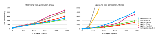
However, we’ve observed that it is possible, and quite valuable, to be able to approximately predict the performance of a Dusa program by reasoning about prefix firings and the deduce-then-choose execution strategy. The left side of Figure 9 shows that the spanning tree generation algorithm (Figure 2) has, across graphs with different features, a running time in Dusa consistently proportional to the number of edges, as the prefix firing methodology would predict. The right side of Figure 9 shows the performance of our best Clingo implementation of the same spec. (Appendix B contains much more comparison of Dusa’s performance relative to Clingo and Alpha on a variety of programs.)

7. Future work

The most obvious future work is completing a proof of 5.22, which would allow us to combine the results of Sections 3 and 5 to declare that we have a satisfying denotational semantics for answer set programming. We believe that a mechanized development of the results presented and referenced in this paper would aid in proving both 5.22 relating the denotational and operational semantics and 6.5 establishing the nondeterministic completeness of Algorithm 2.

7.1. Proof theory

In the authors’ estimation, there are three satisfying approaches to arriving at the meaning of a logic programming language. The first approach is the most ubiquitous: the meaning of a logic program is the least fixed point of a monontonic immediate consequence operator. The second is a direct appeal to models in classical logic, as in Clark’s completion, which has the obvious problems with self-justifying deduction described in the introduction. A third approach defines solutions to logic programs in terms of provability in a constructive proof theory (Miller et al., 1991), though there’s almost no work on justifying negation in this setting. An advantage of the proof-based approach is that proofs represent evidence for every derived fact (which, for finite-choice logic programming, might include evidence of absence), yielding context-dependent utility such as audit trails and explainability for solutions. For this and other reasons, we are interested in investigating proof theory for finite-choice logic programs.

7.2. Stratified negation

Answer set programming produces a canonical model on locally stratified answer set programs, so we can already simulate stratified negation via the translation in Section 3. However, this is often not ideal: if we want to know whether an edge in a sparse graph exists or not, finite-choice logic programming as presented here must materialize the dense graph of edges-that-do-not-exist. This expensive step is not necessary in datalog with stratified negation.

Stratification is not just for negation: it would also allow programs to talk about aggregate values such as the sum of the weights on the edges of a spanning tree. We also speculate that using stratification to inform the order in which attributes are considered in Algorithm 2 would lead to exponential speedups in many cases.

7.3. Eliminating backtracking points

The backtracking structure of our Algorithm 2 as illustrated in Figure 8 is notably reminiscent of the DPLL algorithm for solving the CNF-SAT problems. Under this analogy, the deduce-then-choose strategy can be seen as a form of unit propagation. However, it is a weak form of unit propagation, as conflicts can be easily hidden behind some trivial deduction. Speculatively performing deduction to eliminate inconsistent branches before adding a backtracking point can potentially eliminate an exponential amount of backtracking.

7.4. Avoiding searching for non-solution models

Algorithm 2 is an algorithm that searches for models of a program, but we are interested in the solutions, which are only the definite models. This can lead to problems, such as the following program:

(48) 𝑛𝑎𝑡(x)𝑛𝑎𝑡𝑥\displaystyle{{{\color[rgb]{.5,.5,.5}\definecolor[named]{pgfstrokecolor}{rgb}{.5,.5,.5}\pgfsys@color@gray@stroke{.5}\pgfsys@color@gray@fill{.5}\mathit{nat}}(x)}} 𝑛𝑎𝑡(𝗌(x))absent𝑛𝑎𝑡𝗌𝑥\displaystyle\leftarrow{{{\color[rgb]{.5,.5,.5}\definecolor[named]{pgfstrokecolor}{rgb}{.5,.5,.5}\pgfsys@color@gray@stroke{.5}\pgfsys@color@gray@fill{.5}\mathit{nat}}({\color[rgb]{0,.5,.5}\definecolor[named]{pgfstrokecolor}{rgb}{0,.5,.5}\mathsf{s}}(x))}}
(49) p(x)is?¯𝗍𝗍𝑝𝑥¯is?𝗍𝗍\displaystyle{{{\color[rgb]{.5,.5,.5}\definecolor[named]{pgfstrokecolor}{rgb}{.5,.5,.5}\pgfsys@color@gray@stroke{.5}\pgfsys@color@gray@fill{.5}\mathit{p}}({x})}\operatorname{{\color[rgb]{0,0,1}\definecolor[named]{pgfstrokecolor}{rgb}{0,0,1}{\underline{\textrm{{is?}}}}}}{{{\color[rgb]{0,.5,.5}\definecolor[named]{pgfstrokecolor}{rgb}{0,.5,.5}\mathsf{tt}}}}} 𝑛𝑎𝑡(x)absent𝑛𝑎𝑡𝑥\displaystyle\leftarrow{{{\color[rgb]{.5,.5,.5}\definecolor[named]{pgfstrokecolor}{rgb}{.5,.5,.5}\pgfsys@color@gray@stroke{.5}\pgfsys@color@gray@fill{.5}\mathit{nat}}(x)}}

Seeded with the fact 𝑛𝑎𝑡(𝗌n(𝗓))𝑛𝑎𝑡superscript𝗌𝑛𝗓{{{\color[rgb]{.5,.5,.5}\definecolor[named]{pgfstrokecolor}{rgb}{.5,.5,.5}\pgfsys@color@gray@stroke{.5}\pgfsys@color@gray@fill{.5}\mathit{nat}}({\color[rgb]{0,.5,.5}\definecolor[named]{pgfstrokecolor}{rgb}{0,.5,.5}\mathsf{s}}^{n}({\color[rgb]{0,.5,.5}\definecolor[named]{pgfstrokecolor}{rgb}{0,.5,.5}\mathsf{z}}))}}, this program has $2^{n}$ indefinite models but only 1 definite model. The effect in our current implementation is that, if we seek to enumerate all solutions to this program, execution will immediately return the one definite model (due to the bias against negative-information branches) and will then appear to hang as the exponentially many indefinite models are considered and rejected in turn. In situations like this, an algorithm that is incomplete for models, but complete for solutions, is desirable and would lead to an exponential improvement in enumerating all solutions.

7.5. Richer partial orders

In order to account for negative information in our semantics, the value associated with an attribute went from being a discrete term to being a member of the $\mathit{Constraint}$ poset. It may be possible to utilize this generalization to increase the language’s expressiveness with an analogue of LVars (Kuper and Newton, 2013). For example, we might allow an integer-valued attribute to be given successively larger values, so long as premises only check whether that attribute has a value greater than or equal to some threshold.

8. Conclusion

We have introduced the theory and implementation of finite-choice logic programming, an approach to logic programming where the meaning of programs that admit multiple models is defined as the least fixed point of a monotonic immediate consequence operator, albeit in a novel domain of mutually-exclusive models.

Finite-choice logic programming also provides a way of characterizing the stable models of non-ground answer set programs directly in terms of the operational semantics in Section 2.

Our Dusa implementation can enumerate solutions to finite-choice logic programs, and the runtime behavior of our implementation can reliably (if approximately) be predicted by McAllester’s cost semantics based on prefix firings.

Acknowledgements.
The first author carried out the bulk of design and implementation work on this project during a batch at Recurse Center. We are grateful to Recurse for providing a community and structure to support thinking deeply about programming. We want to thank Ian Horswill, whose CatSAT project (Horswill, 2018) was an important inspiration for this work, as well as Richard Comploi-Taupe, who helped us understand the state of answer set programming with lazy grounding. Thanks to Mitch Wand and to three anonymous reviewers whose comments helped us to improve this draft. This work was partially supported by the National Science Foundation under Grant No. 1846122.

References

  • (1)
  • Alvaro et al. (2011a) Peter Alvaro, Tom J Ameloot, Joseph M Hellerstein, William Marczak, and Jan Van den Bussche. 2011a. A declarative semantics for Dedalus. UC Berkeley EECS Technical Report 120 (2011), 2011.
  • Alvaro et al. (2011b) Peter Alvaro, William R Marczak, Neil Conway, Joseph M Hellerstein, David Maier, and Russell Sears. 2011b. Dedalus: Datalog in time and space. In Datalog Reloaded: First International Workshop. Revised Selected Papers. Springer, Oxford, UK, 262–281.
  • Aref et al. (2015) Molham Aref, Balder ten Cate, Todd J. Green, Benny Kimelfeld, Dan Olteanu, Emir Pasalic, Todd L. Veldhuizen, and Geoffrey Washburn. 2015. Design and Implementation of the LogicBlox System. In Proceedings of the 2015 ACM SIGMOD International Conference on Management of Data (Melbourne, Victoria, Australia) (SIGMOD ’15). Association for Computing Machinery, New York, NY, USA, 1371–1382. https://doi.org/10.1145/2723372.2742796
  • Claessen and Hughes (2011) Koen Claessen and John Hughes. 2011. QuickCheck: a lightweight tool for random testing of Haskell programs. ACM SIGPLAN Notices 46, 4 (2011), 53–64.
  • Clark (1978) Keith L. Clark. 1978. Negation as Failure. In Logic and Data Bases, Hervé Gallaire and Jack Minker (Eds.). Springer US, Boston, MA, 293–322. https://doi.org/10.1007/978-1-4684-3384-5_11
  • Comploi-Taupe et al. (2023) Richard Comploi-Taupe, Gerhard Friedrich, Konstantin Schekotihin, and Antonius Weinzierl. 2023. Domain-Specific Heuristics in Answer Set Programming: A Declarative Non-Monotonic Approach. J. Artif. Int. Res. 76 (may 2023), 56 pages. https://doi.org/10.1613/jair.1.14091
  • Dabral and Martens (2020) Chinmaya Dabral and Chris Martens. 2020. Generating explorable narrative spaces with answer set programming. In Proceedings of the AAAI Conference on Artificial Intelligence and Interactive Digital Entertainment, Vol. 16. AAAI Press, Washington, USA, 45–51.
  • Dabral et al. (2023) Chinmaya Dabral, Emma Tosch, and Chris Martens. 2023. Exploring Consequences of Privacy Policies with Narrative Generation via Answer Set Programming. (2023). Presented at Workshop on Programming Languages and the Law (ProLaLa@POPL). Preprint: https://arxiv.org/abs/2212.06719.
  • Dal Palù et al. (2009) Alessandro Dal Palù, Agostino Dovier, Enrico Pontelli, and Gianfranco Rossi. 2009. GASP: Answer Set Programming with Lazy Grounding. Fundam. Inf. 96, 3 (2009), 297–322.
  • Dao-Tran et al. (2012) Minh Dao-Tran, Thomas Eiter, Michael Fink, Gerald Weidinger, and Antonius Weinzierl. 2012. OMiGA : An Open Minded Grounding On-The-Fly Answer Set Solver. In Logics in Artificial Intelligence, Luis Fariñas del Cerro, Andreas Herzig, and Jérôme Mengin (Eds.). Springer Berlin Heidelberg, Berlin, Heidelberg, 480–483.
  • Dormans and Bakkes (2011) Joris Dormans and Sander Bakkes. 2011. Generating missions and spaces for adaptable play experiences. IEEE Transactions on Computational Intelligence and AI in Games 3, 3 (2011), 216–228.
  • Eisner (2023) Jason Eisner. 2023. Time-and-Space-Efficient Weighted Deduction. Transactions of the Association for Computational Linguistics 11 (08 2023), 960–973. https://doi.org/10.1162/tacl_a_00588 arXiv:https://direct.mit.edu/tacl/article-pdf/doi/10.1162/tacl_a_00588/2154459/tacl_a_00588.pdf
  • Eiter et al. (1997) Thomas Eiter, Georg Gottlob, and Heikki Mannila. 1997. Disjunctive datalog. ACM Transactions on Database Systems (TODS) 22, 3 (1997), 364–418.
  • Gebser et al. (2017) Martin Gebser, Roland Kaminski, Benjamin Kaufmann, and Torsten Schaub. 2017. Multi-shot ASP solving with clingo. CoRR abs/1705.09811 (2017).
  • Gebser et al. (2011) Martin Gebser, Benjamin Kaufmann, Roland Kaminski, Max Ostrowski, Torsten Schaub, and Marius Schneider. 2011. Potassco: The Potsdam answer set solving collection. Ai Communications 24, 2 (2011), 107–124.
  • Gelfond and Lifschitz (1988) Michael Gelfond and Vladimir Lifschitz. 1988. The Stable Model Semantics for Logic Programming. In Proceedings of International Logic Programming Conference and Symposium, Robert Kowalski and Kenneth A. Bowen (Eds.). MIT Press, 1070–1080.
  • Giannotti et al. (2001) Fosca Giannotti, Dino Pedreschi, and Carlo Zaniolo. 2001. Semantics and Expressive Power of Nondeterministic Constructs in Deductive Databases. J. Comput. System Sci. 62, 1 (2001), 15–42. https://doi.org/10.1006/jcss.1999.1699
  • Goldstein et al. (2023) Harrison Goldstein, Samantha Frohlich, Meng Wang, and Benjamin C Pierce. 2023. Reflecting on Random Generation. Proceedings of the ACM on Programming Languages 7, ICFP (2023), 322–355.
  • Goldstein and Pierce (2022) Harrison Goldstein and Benjamin C Pierce. 2022. Parsing randomness. Proceedings of the ACM on Programming Languages 6, OOPSLA2 (2022), 89–113.
  • Greco and Zaniolo (2001) Sergio Greco and Carlo Zaniolo. 2001. Greedy algorithms in Datalog. Theory and Practice of Logic Programming 1, 4 (2001), 381–407. https://doi.org/10.1017/S1471068401001090
  • Horswill (2018) Ian Horswill. 2018. CatSAT: A Practical, Embedded, SAT Language for Runtime PCG. Proceedings of the AAAI Conference on Artificial Intelligence and Interactive Digital Entertainment 14, 1 (Sep. 2018), 38–44. https://doi.org/10.1609/aiide.v14i1.13026
  • Hu et al. (2021) Xiaowen Hu, Joshua Karp, David Zhao, Abdul Zreika, Xi Wu, and Bernhard Scholz. 2021. The Choice Construct in the Soufflé Language. In Programming Languages and Systems, Hakjoo Oh (Ed.). Springer International Publishing, Cham, 163–181.
  • Kennaway and Hoare (1980) JR Kennaway and CAR Hoare. 1980. A theory of nondeterminism. In Automata, Languages and Programming: Seventh Colloquium Noordwijkerhout, the Netherlands July 14–18, 1980 7. Springer, 338–350.
  • Komendantskaya and Seda (2009) Ekaterina Komendantskaya and Anthony Karel Seda. 2009. Sound and Complete SLD-Resolution for Bilattice-Based Annotated Logic Programs. Electronic Notes in Theoretical Computer Science 225 (2009), 141–159. https://doi.org/10.1016/j.entcs.2008.12.071 Proceedings of the Irish Conference on the Mathematical Foundations of Computer Science and Information Technology (MFCSIT 2006).
  • Krishnamurthy and Naqvi (1988) Ravi Krishnamurthy and Shamim Naqvi. 1988. Non-Deterministic Choice in Datalog. In Proceedings of the Third International Conference on Data and Knowledge Bases, C. BEERI, J.W. SCHMIDT, and U. DAYAL (Eds.). Morgan Kaufmann, 416–424. https://doi.org/10.1016/B978-1-4832-1313-2.50038-X
  • Kuper and Newton (2013) Lindsey Kuper and Ryan R. Newton. 2013. LVars: lattice-based data structures for deterministic parallelism. In Proceedings of the 2nd ACM SIGPLAN Workshop on Functional High-Performance Computing (Boston, Massachusetts, USA) (FHPC ’13). Association for Computing Machinery, New York, NY, USA, 71–84. https://doi.org/10.1145/2502323.2502326
  • Lampropoulos et al. (2017) Leonidas Lampropoulos, Zoe Paraskevopoulou, and Benjamin C Pierce. 2017. Generating good generators for inductive relations. Proceedings of the ACM on Programming Languages 2, POPL (2017), 1–30.
  • Lefévre et al. (2017) Claire Lefévre, Christopher Béatrix, Igor Stéphan, and Laurent Garcia. 2017. ASPeRiX, a first-order forward chaining approach for answer set computing. Theory and Practice of Logic Programming 17, 3 (2017), 266–310. https://doi.org/10.1017/S1471068416000569
  • Leone et al. (1997) Nicola Leone, Pasquale Rullo, and Francesco Scarcello. 1997. Disjunctive stable models: Unfounded sets, fixpoint semantics, and computation. Information and computation 135, 2 (1997), 69–112.
  • Lifschitz (2019) Vladimir Lifschitz. 2019. Answer set programming. Springer Heidelberg.
  • McAllester (2002) David McAllester. 2002. On the complexity analysis of static analyses. J. ACM 49, 4 (jul 2002), 512–537. https://doi.org/10.1145/581771.581774
  • Miller et al. (1991) Dale Miller, Gopalan Nadathur, Frank Pfenning, and Andre Scedrov. 1991. Uniform proofs as a foundation for logic programming. Annals of Pure and Applied Logic 51, 1 (1991), 125–157. https://doi.org/10.1016/0168-0072(91)90068-W
  • Neufeld et al. (2015) Xenija Neufeld, Sanaz Mostaghim, and Diego Perez-Liebana. 2015. Procedural level generation with answer set programming for general video game playing. In 2015 7th Computer Science and Electronic Engineering Conference (CEEC). IEEE, 207–212.
  • Paraskevopoulou et al. (2022) Zoe Paraskevopoulou, Aaron Eline, and Leonidas Lampropoulos. 2022. Computing correctly with inductive relations. In Proceedings of the 43rd ACM SIGPLAN International Conference on Programming Language Design and Implementation. ACM, NY, USA, 966–980.
  • Plotkin (1976) Gordon D Plotkin. 1976. A powerdomain construction. SIAM J. Comput. 5, 3 (1976), 452–487.
  • Przymusinski (1988) Teodor C. Przymusinski. 1988. On the Declarative Semantics of Deductive Databases and Logic Programs. In Foundations of Deductive Databases and Logic Programming, Jack Minker (Ed.). Morgan Kaufmann, 193–216. https://doi.org/10.1016/B978-0-934613-40-8.50009-9
  • Przymusinski (1991) Teodor C Przymusinski. 1991. Stable semantics for disjunctive programs. New generation computing 9, 3-4 (1991), 401–424.
  • Sacca and Zaniolo (1990) Domenico Sacca and Carlo Zaniolo. 1990. Stable models and non-determinism in logic programs with negation. In Proceedings of the Ninth ACM SIGACT-SIGMOD-SIGART Symposium on Principles of Database Systems (Nashville, USA) (PODS ’90). Association for Computing Machinery, New York, NY, USA, 205–217. https://doi.org/10.1145/298514.298572
  • Scott (1982) Dana S Scott. 1982. Domains for denotational semantics. In Automata, Languages and Programming: Ninth Colloquium Aarhus, Denmark, July 12–16, 1982 9. Springer, 577–610.
  • Seidel et al. (2015) Eric L Seidel, Niki Vazou, and Ranjit Jhala. 2015. Type targeted testing. In Programming Languages and Systems: 24th European Symposium on Programming, ESOP 2015, Held as Part of the European Joint Conferences on Theory and Practice of Software, ETAPS 2015, London, UK, April 11-18, 2015, Proceedings 24. Springer, 812–836.
  • Shaker et al. (2016) Noor Shaker, Julian Togelius, and Mark J Nelson. 2016. Procedural content generation in games. Springer.
  • Short and Adams (2017) Tanya Short and Tarn Adams. 2017. Procedural generation in game design. CRC Press.
  • Simmons and Pfenning (2008) Robert J. Simmons and Frank Pfenning. 2008. Linear Logical Algorithms. In Automata, Languages and Programming, Luca Aceto, Ivan Damgård, Leslie Ann Goldberg, Magnús M. Halldórsson, Anna Ingólfsdóttir, and Igor Walukiewicz (Eds.). Springer Berlin Heidelberg, Berlin, Heidelberg, 336–347.
  • Smith and Bryson (2014) Anthony J Smith and Joanna J Bryson. 2014. A logical approach to building dungeons: Answer set programming for hierarchical procedural content generation in roguelike games. In Proceedings of the 50th Anniversary Convention of the AISB.
  • Smith et al. (2013) Adam M Smith, Eric Butler, and Zoran Popovic. 2013. Quantifying over play: Constraining undesirable solutions in puzzle design. In Foundations of Digital Games. 221–228.
  • Smith and Mateas (2011) Adam M Smith and Michael Mateas. 2011. Answer set programming for procedural content generation: A design space approach. IEEE Transactions on Computational Intelligence and AI in Games 3, 3 (2011), 187–200.
  • Smyth (1976) Michael B Smyth. 1976. Powerdomains. In International Symposium on Mathematical Foundations of Computer Science. Springer, 537–543.
  • Summerville et al. (2018) Adam Summerville, Chris Martens, Ben Samuel, Joseph Osborn, Noah Wardrip-Fruin, and Michael Mateas. 2018. Gemini: Bidirectional generation and analysis of games via ASP. In Fourteenth Artificial Intelligence and Interactive Digital Entertainment Conference.
  • Tarski (1955) Alfred Tarski. 1955. A lattice-theoretical fixpoint theorem and its applications. Pacific J. Math 5 (1955), 285–309.
  • Van Gelder et al. (1991) Allen Van Gelder, Kenneth A. Ross, and John S. Schlipf. 1991. The Well-Founded Semantics for General Logic Programs. J. ACM 38, 3 (jul 1991), 619–649. https://doi.org/10.1145/116825.116838
  • Weinzierl (2017) Antonius Weinzierl. 2017. Blending Lazy-Grounding and CDNL Search for Answer-Set Solving. In Logic Programming and Nonmonotonic Reasoning, Marcello Balduccini and Tomi Janhunen (Eds.). Springer International Publishing, Cham, 191–204.

Appendix A Additional proofs

A.1. Connecting finite-choice logic programming to datalog

Proposition A.1.

If the model of a datalog program is finite, it is possible to derive a sequence of facts X𝗌𝖾𝗊=p1(t1¯),,pn(tn¯)subscript𝑋𝗌𝖾𝗊subscript𝑝1¯subscript𝑡1subscript𝑝𝑛¯subscript𝑡𝑛X_{\mathsf{seq}}={{{\color[rgb]{.5,.5,.5}\definecolor[named]{pgfstrokecolor}{rgb}{.5,.5,.5}\pgfsys@color@gray@stroke{.5}\pgfsys@color@gray@fill{.5}\mathit{p_{1}}}(\overline{t_{1}})}},\ldots,{{{\color[rgb]{.5,.5,.5}\definecolor[named]{pgfstrokecolor}{rgb}{.5,.5,.5}\pgfsys@color@gray@stroke{.5}\pgfsys@color@gray@fill{.5}\mathit{p_{n}}}(\overline{t_{n}})}}, such that pi(ti¯)subscript𝑝𝑖¯subscript𝑡𝑖{{{\color[rgb]{.5,.5,.5}\definecolor[named]{pgfstrokecolor}{rgb}{.5,.5,.5}\pgfsys@color@gray@stroke{.5}\pgfsys@color@gray@fill{.5}\mathit{p_{i}}}(\overline{t_{i}})}} is always an immediate consequence of pj(tj)subscript𝑝𝑗subscript𝑡𝑗{{{\color[rgb]{.5,.5,.5}\definecolor[named]{pgfstrokecolor}{rgb}{.5,.5,.5}\pgfsys@color@gray@stroke{.5}\pgfsys@color@gray@fill{.5}\mathit{p_{j}}}(t_{j})}} for $j<i$.

If a datalog model is finite, it can be derived by a finite number of applications of the (datalog) immediate consequence operator, where each application adds a finite number of additional facts. We construct the sequence by placing all the facts derived with the first application of the immediate consequence operator first, followed by any additional facts derived with the second application of the immediate consequence operator, and so on.

Proof of Theorem 3.1 relating datalog and finite-choice logic programming.

Restating the theorem: Let $P$ be a datalog program with a finite model, and let $\langle P\rangle$ be the interpretation of $P$ as a finite-choice logic program as above. Then there is a unique solution $D$ to $\langle P\rangle$, and the model of $P$ is {p(t¯)p(t¯)is¯𝗎𝗇𝗂𝗍D}conditional-set𝑝¯𝑡𝑝¯𝑡¯is𝗎𝗇𝗂𝗍𝐷\{{{{\color[rgb]{.5,.5,.5}\definecolor[named]{pgfstrokecolor}{rgb}{.5,.5,.5}\pgfsys@color@gray@stroke{.5}\pgfsys@color@gray@fill{.5}\mathit{p}}(\overline{t})}}\mid{{{\color[rgb]{.5,.5,.5}\definecolor[named]{pgfstrokecolor}{rgb}{.5,.5,.5}\pgfsys@color@gray@stroke{.5}\pgfsys@color@gray@fill{.5}\mathit{p}}({\overline{t}})}\operatorname{{\color[rgb]{0,0,1}\definecolor[named]{pgfstrokecolor}{rgb}{0,0,1}{\underline{\textrm{{is}}}}}}{{{\color[rgb]{0,.5,.5}\definecolor[named]{pgfstrokecolor}{rgb}{0,.5,.5}\mathsf{unit}}}}}\in D\}.

By Lemma A.1 we can get some sequence X𝗌𝖾𝗊=p1(t1¯),,pn(tn¯)subscript𝑋𝗌𝖾𝗊subscript𝑝1¯subscript𝑡1subscript𝑝𝑛¯subscript𝑡𝑛X_{\mathsf{seq}}={{{\color[rgb]{.5,.5,.5}\definecolor[named]{pgfstrokecolor}{rgb}{.5,.5,.5}\pgfsys@color@gray@stroke{.5}\pgfsys@color@gray@fill{.5}\mathit{p_{1}}}(\overline{t_{1}})}},\ldots,{{{\color[rgb]{.5,.5,.5}\definecolor[named]{pgfstrokecolor}{rgb}{.5,.5,.5}\pgfsys@color@gray@stroke{.5}\pgfsys@color@gray@fill{.5}\mathit{p_{n}}}(\overline{t_{n}})}} containing exactly the elements in the model of $P$, where pi(ti¯)subscript𝑝𝑖¯subscript𝑡𝑖{{{\color[rgb]{.5,.5,.5}\definecolor[named]{pgfstrokecolor}{rgb}{.5,.5,.5}\pgfsys@color@gray@stroke{.5}\pgfsys@color@gray@fill{.5}\mathit{p_{i}}}(\overline{t_{i}})}} is always an immediate consequence of the set of facts that precede it in the sequence.

By induction on $n$ we get that {}P{pi(ti¯)is¯𝗎𝗇𝗂𝗍i<npi(ti¯)X𝗌𝖾𝗊}subscriptsuperscriptleads-todelimited-⟨⟩𝑃conditionalsubscript𝑝𝑖¯subscript𝑡𝑖¯is𝗎𝗇𝗂𝗍𝑖𝑛subscript𝑝𝑖¯subscript𝑡𝑖subscript𝑋𝗌𝖾𝗊\{\}\operatorname{\leadsto}^{*}_{\langle P\rangle}\{{{{\color[rgb]{.5,.5,.5}\definecolor[named]{pgfstrokecolor}{rgb}{.5,.5,.5}\pgfsys@color@gray@stroke{.5}\pgfsys@color@gray@fill{.5}\mathit{p_{i}}}({\overline{t_{i}}})}\operatorname{{\color[rgb]{0,0,1}\definecolor[named]{pgfstrokecolor}{rgb}{0,0,1}{\underline{\textrm{{is}}}}}}{{{\color[rgb]{0,.5,.5}\definecolor[named]{pgfstrokecolor}{rgb}{0,.5,.5}\mathsf{unit}}}}}\mid i<n\wedge{{{\color[rgb]{.5,.5,.5}\definecolor[named]{pgfstrokecolor}{rgb}{.5,.5,.5}\pgfsys@color@gray@stroke{.5}\pgfsys@color@gray@fill{.5}\mathit{p_{i}}}(\overline{t_{i}})}}\in X_{\mathsf{seq}}\}. Each new fact in the sequence is derived from some rule in the datalog program, and we can match that transition with the translated constructive answer set program. The solution $D$ we needed to construct is then {pi(ti¯)is¯𝗎𝗇𝗂𝗍pi(ti¯)X𝗌𝖾𝗊}conditional-setsubscript𝑝𝑖¯subscript𝑡𝑖¯is𝗎𝗇𝗂𝗍subscript𝑝𝑖¯subscript𝑡𝑖subscript𝑋𝗌𝖾𝗊\{{{{\color[rgb]{.5,.5,.5}\definecolor[named]{pgfstrokecolor}{rgb}{.5,.5,.5}\pgfsys@color@gray@stroke{.5}\pgfsys@color@gray@fill{.5}\mathit{p_{i}}}({\overline{t_{i}}})}\operatorname{{\color[rgb]{0,0,1}\definecolor[named]{pgfstrokecolor}{rgb}{0,0,1}{\underline{\textrm{{is}}}}}}{{{\color[rgb]{0,.5,.5}\definecolor[named]{pgfstrokecolor}{rgb}{0,.5,.5}\mathsf{unit}}}}}\mid{{{\color[rgb]{.5,.5,.5}\definecolor[named]{pgfstrokecolor}{rgb}{.5,.5,.5}\pgfsys@color@gray@stroke{.5}\pgfsys@color@gray@fill{.5}\mathit{p_{i}}}(\overline{t_{i}})}}\in X_{\mathsf{seq}}\}.

We need to show that $D$ is a solution, which means it has to be saturated and consistent. It’s obviously consistent: inconsistencies are impossible when every attribute maps to $\mathsf{unit}$. To show that it is saturated, we assume some additional fact p(t¯)is¯𝗎𝗇𝗂𝗍𝑝¯𝑡¯is𝗎𝗇𝗂𝗍{{{\color[rgb]{.5,.5,.5}\definecolor[named]{pgfstrokecolor}{rgb}{.5,.5,.5}\pgfsys@color@gray@stroke{.5}\pgfsys@color@gray@fill{.5}\mathit{p}}({\overline{t}})}\operatorname{{\color[rgb]{0,0,1}\definecolor[named]{pgfstrokecolor}{rgb}{0,0,1}{\underline{\textrm{{is}}}}}}{{{\color[rgb]{0,.5,.5}\definecolor[named]{pgfstrokecolor}{rgb}{0,.5,.5}\mathsf{unit}}}}} could be derived. Were that to be the case, there would be a corresponding rule that would add p(t¯)𝑝¯𝑡{{{\color[rgb]{.5,.5,.5}\definecolor[named]{pgfstrokecolor}{rgb}{.5,.5,.5}\pgfsys@color@gray@stroke{.5}\pgfsys@color@gray@fill{.5}\mathit{p}}(\overline{t})}} to $X_{\mathsf{seq}}$, contradicting the assumption that $X_{\mathsf{seq}}$ contains exactly the elements of $P$’s unique model.

It remains to be shown that $D$ is the unique solution. Consider an arbitrary solution $D^{\prime}$. First, by induction on the derivation of the solution p(t¯)is¯vD𝑝¯𝑡¯is𝑣𝐷{{{\color[rgb]{.5,.5,.5}\definecolor[named]{pgfstrokecolor}{rgb}{.5,.5,.5}\pgfsys@color@gray@stroke{.5}\pgfsys@color@gray@fill{.5}\mathit{p}}({\overline{t}})}\operatorname{{\color[rgb]{0,0,1}\definecolor[named]{pgfstrokecolor}{rgb}{0,0,1}{\underline{\textrm{{is}}}}}}{{v}}}\in D it must be the case that $v={\color[rgb]{0,.5,.5}\definecolor[named]{pgfstrokecolor}{rgb}{0,.5,.5}\mathsf{unit}}$. If $D^{\prime}$ was missing any elements in $D$ then it wouldn’t be a solution, and if $D$ was missing any elements in $D^{\prime}$ we could use that to show that $X_{\mathsf{seq}}$ was missing some element in $P$’s unique model, so $D=D^{\prime}$. ∎

A.2. Connecting finite-choice logic programming to answer set programming

Proof of Theorem 3.2 part 1, finite-choice logic programming finds all stable models.

Restating the theorem: Let $P$ be an ASP program, and let $\langle P\rangle$ be the interpretation of $P$ as a finite-choice logic program as defined above. For all stable models $X$ of $P$, there exists a solution $D$ of $\langle P\rangle$ such that pis¯𝗍𝗍D𝑝¯is𝗍𝗍𝐷{{{\color[rgb]{.5,.5,.5}\definecolor[named]{pgfstrokecolor}{rgb}{.5,.5,.5}\pgfsys@color@gray@stroke{.5}\pgfsys@color@gray@fill{.5}\mathit{p}}}\operatorname{{\color[rgb]{0,0,1}\definecolor[named]{pgfstrokecolor}{rgb}{0,0,1}{\underline{\textrm{{is}}}}}}{{{\color[rgb]{0,.5,.5}\definecolor[named]{pgfstrokecolor}{rgb}{0,.5,.5}\mathsf{tt}}}}}\in D if and only if pX𝑝𝑋{\color[rgb]{.5,.5,.5}\definecolor[named]{pgfstrokecolor}{rgb}{.5,.5,.5}\pgfsys@color@gray@stroke{.5}\pgfsys@color@gray@fill{.5}\mathit{p}}\in X.

Let $X$ be a stable model of $P$. The reduct $P^{X}$ is just a datalog program, so by Proposition A.1 we can get some sequence X𝗌𝖾𝗊=p1,,pksubscript𝑋𝗌𝖾𝗊subscript𝑝1subscript𝑝𝑘X_{\mathsf{seq}}={\color[rgb]{.5,.5,.5}\definecolor[named]{pgfstrokecolor}{rgb}{.5,.5,.5}\pgfsys@color@gray@stroke{.5}\pgfsys@color@gray@fill{.5}\mathit{p_{1}}},\ldots,{\color[rgb]{.5,.5,.5}\definecolor[named]{pgfstrokecolor}{rgb}{.5,.5,.5}\pgfsys@color@gray@stroke{.5}\pgfsys@color@gray@fill{.5}\mathit{p_{k}}} containing exactly the elements of $X$ such that each pisubscript𝑝𝑖{\color[rgb]{.5,.5,.5}\definecolor[named]{pgfstrokecolor}{rgb}{.5,.5,.5}\pgfsys@color@gray@stroke{.5}\pgfsys@color@gray@fill{.5}\mathit{p_{i}}} is the immediate consequence of the preceding facts according to some rule in the reduct $P^{X}$.

The proof below proceeds in two steps. In the first step, we establish by induction that for any prefix p1,,psubscript𝑝1𝑝{\color[rgb]{.5,.5,.5}\definecolor[named]{pgfstrokecolor}{rgb}{.5,.5,.5}\pgfsys@color@gray@stroke{.5}\pgfsys@color@gray@fill{.5}\mathit{p_{1}}},\ldots,{\color[rgb]{.5,.5,.5}\definecolor[named]{pgfstrokecolor}{rgb}{.5,.5,.5}\pgfsys@color@gray@stroke{.5}\pgfsys@color@gray@fill{.5}\mathit{p}} of $X_{\mathsf{seq}}$, there exists a consistent database $D$ such that

  • $\varnothing\operatorname{\leadsto}^{*}_{\langle P\rangle}D$

  • pis¯𝗍𝗍Dsuperscript𝑝¯is𝗍𝗍𝐷{\color[rgb]{.5,.5,.5}\definecolor[named]{pgfstrokecolor}{rgb}{.5,.5,.5}\pgfsys@color@gray@stroke{.5}\pgfsys@color@gray@fill{.5}\mathit{p^{\prime}}}\operatorname{{\color[rgb]{0,0,1}\definecolor[named]{pgfstrokecolor}{rgb}{0,0,1}{\underline{\textrm{{is}}}}}}{\color[rgb]{0,.5,.5}\definecolor[named]{pgfstrokecolor}{rgb}{0,.5,.5}\mathsf{tt}}\in D if and only if pp1,,psuperscript𝑝subscript𝑝1𝑝{\color[rgb]{.5,.5,.5}\definecolor[named]{pgfstrokecolor}{rgb}{.5,.5,.5}\pgfsys@color@gray@stroke{.5}\pgfsys@color@gray@fill{.5}\mathit{p^{\prime}}}\in{\color[rgb]{.5,.5,.5}\definecolor[named]{pgfstrokecolor}{rgb}{.5,.5,.5}\pgfsys@color@gray@stroke{.5}\pgfsys@color@gray@fill{.5}\mathit{p_{1}}},\ldots,{\color[rgb]{.5,.5,.5}\definecolor[named]{pgfstrokecolor}{rgb}{.5,.5,.5}\pgfsys@color@gray@stroke{.5}\pgfsys@color@gray@fill{.5}\mathit{p}}

  • pis¯𝖿𝖿Dsuperscript𝑝¯is𝖿𝖿𝐷{\color[rgb]{.5,.5,.5}\definecolor[named]{pgfstrokecolor}{rgb}{.5,.5,.5}\pgfsys@color@gray@stroke{.5}\pgfsys@color@gray@fill{.5}\mathit{p^{\prime}}}\operatorname{{\color[rgb]{0,0,1}\definecolor[named]{pgfstrokecolor}{rgb}{0,0,1}{\underline{\textrm{{is}}}}}}{\color[rgb]{0,.5,.5}\definecolor[named]{pgfstrokecolor}{rgb}{0,.5,.5}\mathsf{ff}}\in D only if pXsuperscript𝑝𝑋{\color[rgb]{.5,.5,.5}\definecolor[named]{pgfstrokecolor}{rgb}{.5,.5,.5}\pgfsys@color@gray@stroke{.5}\pgfsys@color@gray@fill{.5}\mathit{p^{\prime}}}\not\in X

Applying this inductive construction to the entire sequence $X_{\mathsf{seq}}$, we get a $D_{1}$ with pis¯𝗍𝗍Dsuperscript𝑝¯is𝗍𝗍𝐷{\color[rgb]{.5,.5,.5}\definecolor[named]{pgfstrokecolor}{rgb}{.5,.5,.5}\pgfsys@color@gray@stroke{.5}\pgfsys@color@gray@fill{.5}\mathit{p^{\prime}}}\operatorname{{\color[rgb]{0,0,1}\definecolor[named]{pgfstrokecolor}{rgb}{0,0,1}{\underline{\textrm{{is}}}}}}{\color[rgb]{0,.5,.5}\definecolor[named]{pgfstrokecolor}{rgb}{0,.5,.5}\mathsf{tt}}\in D if and only if pXsuperscript𝑝𝑋{\color[rgb]{.5,.5,.5}\definecolor[named]{pgfstrokecolor}{rgb}{.5,.5,.5}\pgfsys@color@gray@stroke{.5}\pgfsys@color@gray@fill{.5}\mathit{p^{\prime}}}\in X. In the second step, we add additional facts of the form pis¯𝖿𝖿superscript𝑝¯is𝖿𝖿{{{\color[rgb]{.5,.5,.5}\definecolor[named]{pgfstrokecolor}{rgb}{.5,.5,.5}\pgfsys@color@gray@stroke{.5}\pgfsys@color@gray@fill{.5}\mathit{p^{\prime}}}}\operatorname{{\color[rgb]{0,0,1}\definecolor[named]{pgfstrokecolor}{rgb}{0,0,1}{\underline{\textrm{{is}}}}}}{{{\color[rgb]{0,.5,.5}\definecolor[named]{pgfstrokecolor}{rgb}{0,.5,.5}\mathsf{ff}}}}} to $D_{1}$ until we have a solution $D_{2}$ to $\langle P\rangle$ where pis¯𝗍𝗍D2superscript𝑝¯is𝗍𝗍subscript𝐷2{{{\color[rgb]{.5,.5,.5}\definecolor[named]{pgfstrokecolor}{rgb}{.5,.5,.5}\pgfsys@color@gray@stroke{.5}\pgfsys@color@gray@fill{.5}\mathit{p^{\prime}}}}\operatorname{{\color[rgb]{0,0,1}\definecolor[named]{pgfstrokecolor}{rgb}{0,0,1}{\underline{\textrm{{is}}}}}}{{{\color[rgb]{0,.5,.5}\definecolor[named]{pgfstrokecolor}{rgb}{0,.5,.5}\mathsf{tt}}}}}\in D_{2} if and only if pXsuperscript𝑝𝑋{\color[rgb]{.5,.5,.5}\definecolor[named]{pgfstrokecolor}{rgb}{.5,.5,.5}\pgfsys@color@gray@stroke{.5}\pgfsys@color@gray@fill{.5}\mathit{p^{\prime}}}\in X.

First step: induction over the prefixes of $X_{\mathsf{seq}}$

The base case is immediate for $D=\varnothing$. In the inductive case, we’re given a consistent database $D$ where $\varnothing\operatorname{\leadsto}^{*}_{\langle P\rangle}D$ and where $D$ contains pis¯𝗍𝗍superscript𝑝¯is𝗍𝗍{{{\color[rgb]{.5,.5,.5}\definecolor[named]{pgfstrokecolor}{rgb}{.5,.5,.5}\pgfsys@color@gray@stroke{.5}\pgfsys@color@gray@fill{.5}\mathit{p^{\prime}}}}\operatorname{{\color[rgb]{0,0,1}\definecolor[named]{pgfstrokecolor}{rgb}{0,0,1}{\underline{\textrm{{is}}}}}}{{{\color[rgb]{0,.5,.5}\definecolor[named]{pgfstrokecolor}{rgb}{0,.5,.5}\mathsf{tt}}}}} for every psuperscript𝑝{\color[rgb]{.5,.5,.5}\definecolor[named]{pgfstrokecolor}{rgb}{.5,.5,.5}\pgfsys@color@gray@stroke{.5}\pgfsys@color@gray@fill{.5}\mathit{p^{\prime}}} preceding p𝑝{\color[rgb]{.5,.5,.5}\definecolor[named]{pgfstrokecolor}{rgb}{.5,.5,.5}\pgfsys@color@gray@stroke{.5}\pgfsys@color@gray@fill{.5}\mathit{p}} in $X_{\mathsf{seq}}$. We need to show that $\varnothing\operatorname{\leadsto}^{*}_{\langle P\rangle}D^{\prime}$ for some consistent $D^{\prime}$ that additionally contains pis¯𝗍𝗍𝑝¯is𝗍𝗍{{{\color[rgb]{.5,.5,.5}\definecolor[named]{pgfstrokecolor}{rgb}{.5,.5,.5}\pgfsys@color@gray@stroke{.5}\pgfsys@color@gray@fill{.5}\mathit{p}}}\operatorname{{\color[rgb]{0,0,1}\definecolor[named]{pgfstrokecolor}{rgb}{0,0,1}{\underline{\textrm{{is}}}}}}{{{\color[rgb]{0,.5,.5}\definecolor[named]{pgfstrokecolor}{rgb}{0,.5,.5}\mathsf{tt}}}}} (and no additional facts of the form pis¯𝗍𝗍superscript𝑝¯is𝗍𝗍{{{\color[rgb]{.5,.5,.5}\definecolor[named]{pgfstrokecolor}{rgb}{.5,.5,.5}\pgfsys@color@gray@stroke{.5}\pgfsys@color@gray@fill{.5}\mathit{p^{\prime}}}}\operatorname{{\color[rgb]{0,0,1}\definecolor[named]{pgfstrokecolor}{rgb}{0,0,1}{\underline{\textrm{{is}}}}}}{{{\color[rgb]{0,.5,.5}\definecolor[named]{pgfstrokecolor}{rgb}{0,.5,.5}\mathsf{tt}}}}}).

When we derive p𝑝{\color[rgb]{.5,.5,.5}\definecolor[named]{pgfstrokecolor}{rgb}{.5,.5,.5}\pgfsys@color@gray@stroke{.5}\pgfsys@color@gray@fill{.5}\mathit{p}} in the reduct, we know that this was due to a rule pp1,,pn𝑝subscript𝑝1subscript𝑝𝑛{\color[rgb]{.5,.5,.5}\definecolor[named]{pgfstrokecolor}{rgb}{.5,.5,.5}\pgfsys@color@gray@stroke{.5}\pgfsys@color@gray@fill{.5}\mathit{p}}\leftarrow{\color[rgb]{.5,.5,.5}\definecolor[named]{pgfstrokecolor}{rgb}{.5,.5,.5}\pgfsys@color@gray@stroke{.5}\pgfsys@color@gray@fill{.5}\mathit{p_{1}}},\ldots,{\color[rgb]{.5,.5,.5}\definecolor[named]{pgfstrokecolor}{rgb}{.5,.5,.5}\pgfsys@color@gray@stroke{.5}\pgfsys@color@gray@fill{.5}\mathit{p_{n}}} in the reduct $P^{X}$ such that all the premises p1,,pnsubscript𝑝1subscript𝑝𝑛{\color[rgb]{.5,.5,.5}\definecolor[named]{pgfstrokecolor}{rgb}{.5,.5,.5}\pgfsys@color@gray@stroke{.5}\pgfsys@color@gray@fill{.5}\mathit{p_{1}}},\ldots,{\color[rgb]{.5,.5,.5}\definecolor[named]{pgfstrokecolor}{rgb}{.5,.5,.5}\pgfsys@color@gray@stroke{.5}\pgfsys@color@gray@fill{.5}\mathit{p_{n}}} exist in $X_{\mathsf{seq}}$ before p𝑝{\color[rgb]{.5,.5,.5}\definecolor[named]{pgfstrokecolor}{rgb}{.5,.5,.5}\pgfsys@color@gray@stroke{.5}\pgfsys@color@gray@fill{.5}\mathit{p}}. This rule in the reduct $P^{X}$ was itself derived from a rule pp1,,pn,¬q1,,¬qm𝑝subscript𝑝1subscript𝑝𝑛subscript𝑞1subscript𝑞𝑚{\color[rgb]{.5,.5,.5}\definecolor[named]{pgfstrokecolor}{rgb}{.5,.5,.5}\pgfsys@color@gray@stroke{.5}\pgfsys@color@gray@fill{.5}\mathit{p}}\leftarrow{\color[rgb]{.5,.5,.5}\definecolor[named]{pgfstrokecolor}{rgb}{.5,.5,.5}\pgfsys@color@gray@stroke{.5}\pgfsys@color@gray@fill{.5}\mathit{p_{1}}},\ldots,{\color[rgb]{.5,.5,.5}\definecolor[named]{pgfstrokecolor}{rgb}{.5,.5,.5}\pgfsys@color@gray@stroke{.5}\pgfsys@color@gray@fill{.5}\mathit{p_{n}}},\neg{\color[rgb]{.5,.5,.5}\definecolor[named]{pgfstrokecolor}{rgb}{.5,.5,.5}\pgfsys@color@gray@stroke{.5}\pgfsys@color@gray@fill{.5}\mathit{q_{1}}},\ldots,\neg{\color[rgb]{.5,.5,.5}\definecolor[named]{pgfstrokecolor}{rgb}{.5,.5,.5}\pgfsys@color@gray@stroke{.5}\pgfsys@color@gray@fill{.5}\mathit{q_{m}}} in the original program $P$.

Having found this rule, we define to be $D^{\prime}$ as D{pis¯𝗍𝗍,q1is¯𝖿𝖿,,qmis¯𝖿𝖿}𝐷𝑝¯is𝗍𝗍subscript𝑞1¯is𝖿𝖿subscript𝑞𝑚¯is𝖿𝖿D\cup\{{{{\color[rgb]{.5,.5,.5}\definecolor[named]{pgfstrokecolor}{rgb}{.5,.5,.5}\pgfsys@color@gray@stroke{.5}\pgfsys@color@gray@fill{.5}\mathit{p}}}\operatorname{{\color[rgb]{0,0,1}\definecolor[named]{pgfstrokecolor}{rgb}{0,0,1}{\underline{\textrm{{is}}}}}}{{{\color[rgb]{0,.5,.5}\definecolor[named]{pgfstrokecolor}{rgb}{0,.5,.5}\mathsf{tt}}}}},{{{\color[rgb]{.5,.5,.5}\definecolor[named]{pgfstrokecolor}{rgb}{.5,.5,.5}\pgfsys@color@gray@stroke{.5}\pgfsys@color@gray@fill{.5}\mathit{q_{1}}}}\operatorname{{\color[rgb]{0,0,1}\definecolor[named]{pgfstrokecolor}{rgb}{0,0,1}{\underline{\textrm{{is}}}}}}{{{\color[rgb]{0,.5,.5}\definecolor[named]{pgfstrokecolor}{rgb}{0,.5,.5}\mathsf{ff}}}}},\ldots,{{{\color[rgb]{.5,.5,.5}\definecolor[named]{pgfstrokecolor}{rgb}{.5,.5,.5}\pgfsys@color@gray@stroke{.5}\pgfsys@color@gray@fill{.5}\mathit{q_{m}}}}\operatorname{{\color[rgb]{0,0,1}\definecolor[named]{pgfstrokecolor}{rgb}{0,0,1}{\underline{\textrm{{is}}}}}}{{{\color[rgb]{0,.5,.5}\definecolor[named]{pgfstrokecolor}{rgb}{0,.5,.5}\mathsf{ff}}}}}\}. This immediately satisfies the second condition that pis¯𝗍𝗍Dsuperscript𝑝¯is𝗍𝗍𝐷{\color[rgb]{.5,.5,.5}\definecolor[named]{pgfstrokecolor}{rgb}{.5,.5,.5}\pgfsys@color@gray@stroke{.5}\pgfsys@color@gray@fill{.5}\mathit{p^{\prime}}}\operatorname{{\color[rgb]{0,0,1}\definecolor[named]{pgfstrokecolor}{rgb}{0,0,1}{\underline{\textrm{{is}}}}}}{\color[rgb]{0,.5,.5}\definecolor[named]{pgfstrokecolor}{rgb}{0,.5,.5}\mathsf{tt}}\in D if and only if pp1,,psuperscript𝑝subscript𝑝1𝑝{\color[rgb]{.5,.5,.5}\definecolor[named]{pgfstrokecolor}{rgb}{.5,.5,.5}\pgfsys@color@gray@stroke{.5}\pgfsys@color@gray@fill{.5}\mathit{p^{\prime}}}\in{\color[rgb]{.5,.5,.5}\definecolor[named]{pgfstrokecolor}{rgb}{.5,.5,.5}\pgfsys@color@gray@stroke{.5}\pgfsys@color@gray@fill{.5}\mathit{p_{1}}},\ldots,{\color[rgb]{.5,.5,.5}\definecolor[named]{pgfstrokecolor}{rgb}{.5,.5,.5}\pgfsys@color@gray@stroke{.5}\pgfsys@color@gray@fill{.5}\mathit{p}}, and because the reduct survived into $P^{X}$, we know none of the $q_{i}$ are in $X$, so the third condition that pis¯𝖿𝖿Dsuperscript𝑝¯is𝖿𝖿𝐷{\color[rgb]{.5,.5,.5}\definecolor[named]{pgfstrokecolor}{rgb}{.5,.5,.5}\pgfsys@color@gray@stroke{.5}\pgfsys@color@gray@fill{.5}\mathit{p^{\prime}}}\operatorname{{\color[rgb]{0,0,1}\definecolor[named]{pgfstrokecolor}{rgb}{0,0,1}{\underline{\textrm{{is}}}}}}{\color[rgb]{0,.5,.5}\definecolor[named]{pgfstrokecolor}{rgb}{0,.5,.5}\mathsf{ff}}\in D only if pXsuperscript𝑝𝑋{\color[rgb]{.5,.5,.5}\definecolor[named]{pgfstrokecolor}{rgb}{.5,.5,.5}\pgfsys@color@gray@stroke{.5}\pgfsys@color@gray@fill{.5}\mathit{p^{\prime}}}\not\in X is also satisfied.

We need only extend $\varnothing\operatorname{\leadsto}^{*}_{\langle P\rangle}D$ to construct $\varnothing\operatorname{\leadsto}^{*}_{\langle P\rangle}D^{\prime}$. By the induction hypothesis, piis¯𝗍𝗍subscript𝑝𝑖¯is𝗍𝗍{{{\color[rgb]{.5,.5,.5}\definecolor[named]{pgfstrokecolor}{rgb}{.5,.5,.5}\pgfsys@color@gray@stroke{.5}\pgfsys@color@gray@fill{.5}\mathit{p_{i}}}}\operatorname{{\color[rgb]{0,0,1}\definecolor[named]{pgfstrokecolor}{rgb}{0,0,1}{\underline{\textrm{{is}}}}}}{{{\color[rgb]{0,.5,.5}\definecolor[named]{pgfstrokecolor}{rgb}{0,.5,.5}\mathsf{tt}}}}} is in the database for $1\leq i\leq n$. All but one of those rules are open rules with the conclusion qiis?¯𝖿𝖿subscript𝑞𝑖¯is?𝖿𝖿{{{\color[rgb]{.5,.5,.5}\definecolor[named]{pgfstrokecolor}{rgb}{.5,.5,.5}\pgfsys@color@gray@stroke{.5}\pgfsys@color@gray@fill{.5}\mathit{q_{i}}}}\operatorname{{\color[rgb]{0,0,1}\definecolor[named]{pgfstrokecolor}{rgb}{0,0,1}{\underline{\textrm{{is?}}}}}}{{{\color[rgb]{0,.5,.5}\definecolor[named]{pgfstrokecolor}{rgb}{0,.5,.5}\mathsf{ff}}}}} for $1\leq i\leq m$, and we can apply each of them in turn. The structure of the translation requires us to add q1is¯𝖿𝖿subscript𝑞1¯is𝖿𝖿{{{\color[rgb]{.5,.5,.5}\definecolor[named]{pgfstrokecolor}{rgb}{.5,.5,.5}\pgfsys@color@gray@stroke{.5}\pgfsys@color@gray@fill{.5}\mathit{q_{1}}}}\operatorname{{\color[rgb]{0,0,1}\definecolor[named]{pgfstrokecolor}{rgb}{0,0,1}{\underline{\textrm{{is}}}}}}{{{\color[rgb]{0,.5,.5}\definecolor[named]{pgfstrokecolor}{rgb}{0,.5,.5}\mathsf{ff}}}}} first, then q2is¯𝖿𝖿subscript𝑞2¯is𝖿𝖿{{{\color[rgb]{.5,.5,.5}\definecolor[named]{pgfstrokecolor}{rgb}{.5,.5,.5}\pgfsys@color@gray@stroke{.5}\pgfsys@color@gray@fill{.5}\mathit{q_{2}}}}\operatorname{{\color[rgb]{0,0,1}\definecolor[named]{pgfstrokecolor}{rgb}{0,0,1}{\underline{\textrm{{is}}}}}}{{{\color[rgb]{0,.5,.5}\definecolor[named]{pgfstrokecolor}{rgb}{0,.5,.5}\mathsf{ff}}}}}, and so on. Having added all the relevant negative premises, it’s now possible to apply the one translated closed rule that derives pis¯𝗍𝗍𝑝¯is𝗍𝗍{{{\color[rgb]{.5,.5,.5}\definecolor[named]{pgfstrokecolor}{rgb}{.5,.5,.5}\pgfsys@color@gray@stroke{.5}\pgfsys@color@gray@fill{.5}\mathit{p}}}\operatorname{{\color[rgb]{0,0,1}\definecolor[named]{pgfstrokecolor}{rgb}{0,0,1}{\underline{\textrm{{is}}}}}}{{{\color[rgb]{0,.5,.5}\definecolor[named]{pgfstrokecolor}{rgb}{0,.5,.5}\mathsf{tt}}}}}.

Second step: deriving a solution

The database $D_{1}$ we obtained in the first step might not be a solution, because it might not be saturated. In particular, there may be open rules that allow us to derive additional non-contradictory facts pis¯𝖿𝖿superscript𝑝¯is𝖿𝖿{{{\color[rgb]{.5,.5,.5}\definecolor[named]{pgfstrokecolor}{rgb}{.5,.5,.5}\pgfsys@color@gray@stroke{.5}\pgfsys@color@gray@fill{.5}\mathit{p^{\prime}}}}\operatorname{{\color[rgb]{0,0,1}\definecolor[named]{pgfstrokecolor}{rgb}{0,0,1}{\underline{\textrm{{is}}}}}}{{{\color[rgb]{0,.5,.5}\definecolor[named]{pgfstrokecolor}{rgb}{0,.5,.5}\mathsf{ff}}}}}. This would be the case, for example, if our original program looked something like this.

c𝑐\displaystyle{\color[rgb]{.5,.5,.5}\definecolor[named]{pgfstrokecolor}{rgb}{.5,.5,.5}\pgfsys@color@gray@stroke{.5}\pgfsys@color@gray@fill{.5}\mathit{c}} $\displaystyle\leftarrow$
b𝑏\displaystyle{\color[rgb]{.5,.5,.5}\definecolor[named]{pgfstrokecolor}{rgb}{.5,.5,.5}\pgfsys@color@gray@stroke{.5}\pgfsys@color@gray@fill{.5}\mathit{b}} cabsent𝑐\displaystyle\leftarrow{\color[rgb]{.5,.5,.5}\definecolor[named]{pgfstrokecolor}{rgb}{.5,.5,.5}\pgfsys@color@gray@stroke{.5}\pgfsys@color@gray@fill{.5}\mathit{c}}
a𝑎\displaystyle{\color[rgb]{.5,.5,.5}\definecolor[named]{pgfstrokecolor}{rgb}{.5,.5,.5}\pgfsys@color@gray@stroke{.5}\pgfsys@color@gray@fill{.5}\mathit{a}} b,¬d,¬cabsent𝑏𝑑𝑐\displaystyle\leftarrow{\color[rgb]{.5,.5,.5}\definecolor[named]{pgfstrokecolor}{rgb}{.5,.5,.5}\pgfsys@color@gray@stroke{.5}\pgfsys@color@gray@fill{.5}\mathit{b}},\neg{\color[rgb]{.5,.5,.5}\definecolor[named]{pgfstrokecolor}{rgb}{.5,.5,.5}\pgfsys@color@gray@stroke{.5}\pgfsys@color@gray@fill{.5}\mathit{d}},\neg{\color[rgb]{.5,.5,.5}\definecolor[named]{pgfstrokecolor}{rgb}{.5,.5,.5}\pgfsys@color@gray@stroke{.5}\pgfsys@color@gray@fill{.5}\mathit{c}}

In this case, $D_{1}$ would only contain cis¯𝗍𝗍𝑐¯is𝗍𝗍{{{\color[rgb]{.5,.5,.5}\definecolor[named]{pgfstrokecolor}{rgb}{.5,.5,.5}\pgfsys@color@gray@stroke{.5}\pgfsys@color@gray@fill{.5}\mathit{c}}}\operatorname{{\color[rgb]{0,0,1}\definecolor[named]{pgfstrokecolor}{rgb}{0,0,1}{\underline{\textrm{{is}}}}}}{{{\color[rgb]{0,.5,.5}\definecolor[named]{pgfstrokecolor}{rgb}{0,.5,.5}\mathsf{tt}}}}} and bis¯𝗍𝗍𝑏¯is𝗍𝗍{{{\color[rgb]{.5,.5,.5}\definecolor[named]{pgfstrokecolor}{rgb}{.5,.5,.5}\pgfsys@color@gray@stroke{.5}\pgfsys@color@gray@fill{.5}\mathit{b}}}\operatorname{{\color[rgb]{0,0,1}\definecolor[named]{pgfstrokecolor}{rgb}{0,0,1}{\underline{\textrm{{is}}}}}}{{{\color[rgb]{0,.5,.5}\definecolor[named]{pgfstrokecolor}{rgb}{0,.5,.5}\mathsf{tt}}}}}. In order to get a solution database, dis¯𝖿𝖿𝑑¯is𝖿𝖿{{{\color[rgb]{.5,.5,.5}\definecolor[named]{pgfstrokecolor}{rgb}{.5,.5,.5}\pgfsys@color@gray@stroke{.5}\pgfsys@color@gray@fill{.5}\mathit{d}}}\operatorname{{\color[rgb]{0,0,1}\definecolor[named]{pgfstrokecolor}{rgb}{0,0,1}{\underline{\textrm{{is}}}}}}{{{\color[rgb]{0,.5,.5}\definecolor[named]{pgfstrokecolor}{rgb}{0,.5,.5}\mathsf{ff}}}}} would need to be added.

First, we’ll establish that no additional facts of the form pis¯𝗍𝗍𝑝¯is𝗍𝗍{{{\color[rgb]{.5,.5,.5}\definecolor[named]{pgfstrokecolor}{rgb}{.5,.5,.5}\pgfsys@color@gray@stroke{.5}\pgfsys@color@gray@fill{.5}\mathit{p}}}\operatorname{{\color[rgb]{0,0,1}\definecolor[named]{pgfstrokecolor}{rgb}{0,0,1}{\underline{\textrm{{is}}}}}}{{{\color[rgb]{0,.5,.5}\definecolor[named]{pgfstrokecolor}{rgb}{0,.5,.5}\mathsf{tt}}}}} can be added to $D_{1}$. We consider every rule

pis¯{𝗍𝗍}𝑝¯is𝗍𝗍\displaystyle{{{\color[rgb]{.5,.5,.5}\definecolor[named]{pgfstrokecolor}{rgb}{.5,.5,.5}\pgfsys@color@gray@stroke{.5}\pgfsys@color@gray@fill{.5}\mathit{p}}}\operatorname{{\color[rgb]{0,0,1}\definecolor[named]{pgfstrokecolor}{rgb}{0,0,1}{\underline{\textrm{{is}}}}}}{{\{{\color[rgb]{0,.5,.5}\definecolor[named]{pgfstrokecolor}{rgb}{0,.5,.5}\mathsf{tt}}\}}}} p1is¯𝗍𝗍,,pnis¯𝗍𝗍,q1is¯𝖿𝖿,,qmis¯𝖿𝖿absentsubscript𝑝1¯is𝗍𝗍subscript𝑝𝑛¯is𝗍𝗍subscript𝑞1¯is𝖿𝖿subscript𝑞𝑚¯is𝖿𝖿\displaystyle\leftarrow{{{\color[rgb]{.5,.5,.5}\definecolor[named]{pgfstrokecolor}{rgb}{.5,.5,.5}\pgfsys@color@gray@stroke{.5}\pgfsys@color@gray@fill{.5}\mathit{p_{1}}}}\operatorname{{\color[rgb]{0,0,1}\definecolor[named]{pgfstrokecolor}{rgb}{0,0,1}{\underline{\textrm{{is}}}}}}{{{\color[rgb]{0,.5,.5}\definecolor[named]{pgfstrokecolor}{rgb}{0,.5,.5}\mathsf{tt}}}}},\ldots,{{{\color[rgb]{.5,.5,.5}\definecolor[named]{pgfstrokecolor}{rgb}{.5,.5,.5}\pgfsys@color@gray@stroke{.5}\pgfsys@color@gray@fill{.5}\mathit{p_{n}}}}\operatorname{{\color[rgb]{0,0,1}\definecolor[named]{pgfstrokecolor}{rgb}{0,0,1}{\underline{\textrm{{is}}}}}}{{{\color[rgb]{0,.5,.5}\definecolor[named]{pgfstrokecolor}{rgb}{0,.5,.5}\mathsf{tt}}}}},{{{\color[rgb]{.5,.5,.5}\definecolor[named]{pgfstrokecolor}{rgb}{.5,.5,.5}\pgfsys@color@gray@stroke{.5}\pgfsys@color@gray@fill{.5}\mathit{q_{1}}}}\operatorname{{\color[rgb]{0,0,1}\definecolor[named]{pgfstrokecolor}{rgb}{0,0,1}{\underline{\textrm{{is}}}}}}{{{\color[rgb]{0,.5,.5}\definecolor[named]{pgfstrokecolor}{rgb}{0,.5,.5}\mathsf{ff}}}}},\ldots,{{{\color[rgb]{.5,.5,.5}\definecolor[named]{pgfstrokecolor}{rgb}{.5,.5,.5}\pgfsys@color@gray@stroke{.5}\pgfsys@color@gray@fill{.5}\mathit{q_{m}}}}\operatorname{{\color[rgb]{0,0,1}\definecolor[named]{pgfstrokecolor}{rgb}{0,0,1}{\underline{\textrm{{is}}}}}}{{{\color[rgb]{0,.5,.5}\definecolor[named]{pgfstrokecolor}{rgb}{0,.5,.5}\mathsf{ff}}}}}

in the translated program. There are three cases to consider:

  1. (1)

    If pis¯𝗍𝗍D1𝑝¯is𝗍𝗍subscript𝐷1{{{\color[rgb]{.5,.5,.5}\definecolor[named]{pgfstrokecolor}{rgb}{.5,.5,.5}\pgfsys@color@gray@stroke{.5}\pgfsys@color@gray@fill{.5}\mathit{p}}}\operatorname{{\color[rgb]{0,0,1}\definecolor[named]{pgfstrokecolor}{rgb}{0,0,1}{\underline{\textrm{{is}}}}}}{{{\color[rgb]{0,.5,.5}\definecolor[named]{pgfstrokecolor}{rgb}{0,.5,.5}\mathsf{tt}}}}}\in D_{1}, then the rule can’t add any new facts.

  2. (2)

    If pis¯𝗍𝗍D1𝑝¯is𝗍𝗍subscript𝐷1{{{\color[rgb]{.5,.5,.5}\definecolor[named]{pgfstrokecolor}{rgb}{.5,.5,.5}\pgfsys@color@gray@stroke{.5}\pgfsys@color@gray@fill{.5}\mathit{p}}}\operatorname{{\color[rgb]{0,0,1}\definecolor[named]{pgfstrokecolor}{rgb}{0,0,1}{\underline{\textrm{{is}}}}}}{{{\color[rgb]{0,.5,.5}\definecolor[named]{pgfstrokecolor}{rgb}{0,.5,.5}\mathsf{tt}}}}}\not\in D_{1} and the original ASP rule was not eliminated from the reduct $P^{X}$, then pp1,,pn𝑝subscript𝑝1subscript𝑝𝑛{\color[rgb]{.5,.5,.5}\definecolor[named]{pgfstrokecolor}{rgb}{.5,.5,.5}\pgfsys@color@gray@stroke{.5}\pgfsys@color@gray@fill{.5}\mathit{p}}\leftarrow{\color[rgb]{.5,.5,.5}\definecolor[named]{pgfstrokecolor}{rgb}{.5,.5,.5}\pgfsys@color@gray@stroke{.5}\pgfsys@color@gray@fill{.5}\mathit{p_{1}}},\ldots,{\color[rgb]{.5,.5,.5}\definecolor[named]{pgfstrokecolor}{rgb}{.5,.5,.5}\pgfsys@color@gray@stroke{.5}\pgfsys@color@gray@fill{.5}\mathit{p_{n}}} appears in the reduct. Because p𝑝{\color[rgb]{.5,.5,.5}\definecolor[named]{pgfstrokecolor}{rgb}{.5,.5,.5}\pgfsys@color@gray@stroke{.5}\pgfsys@color@gray@fill{.5}\mathit{p}} is not in the model of the reduct, there must be some premise piXsubscript𝑝𝑖𝑋{\color[rgb]{.5,.5,.5}\definecolor[named]{pgfstrokecolor}{rgb}{.5,.5,.5}\pgfsys@color@gray@stroke{.5}\pgfsys@color@gray@fill{.5}\mathit{p_{i}}}\not\in X, meaning piis¯𝗍𝗍Dsubscript𝑝𝑖¯is𝗍𝗍𝐷{{{\color[rgb]{.5,.5,.5}\definecolor[named]{pgfstrokecolor}{rgb}{.5,.5,.5}\pgfsys@color@gray@stroke{.5}\pgfsys@color@gray@fill{.5}\mathit{p_{i}}}}\operatorname{{\color[rgb]{0,0,1}\definecolor[named]{pgfstrokecolor}{rgb}{0,0,1}{\underline{\textrm{{is}}}}}}{{{\color[rgb]{0,.5,.5}\definecolor[named]{pgfstrokecolor}{rgb}{0,.5,.5}\mathsf{tt}}}}}\not\in D, so the rule doesn’t apply and adding additional facts of the form qis¯𝗍𝗍𝑞¯is𝗍𝗍{{{\color[rgb]{.5,.5,.5}\definecolor[named]{pgfstrokecolor}{rgb}{.5,.5,.5}\pgfsys@color@gray@stroke{.5}\pgfsys@color@gray@fill{.5}\mathit{q}}}\operatorname{{\color[rgb]{0,0,1}\definecolor[named]{pgfstrokecolor}{rgb}{0,0,1}{\underline{\textrm{{is}}}}}}{{{\color[rgb]{0,.5,.5}\definecolor[named]{pgfstrokecolor}{rgb}{0,.5,.5}\mathsf{tt}}}}} would not change that.

  3. (3)

    If pis¯𝗍𝗍D1𝑝¯is𝗍𝗍subscript𝐷1{{{\color[rgb]{.5,.5,.5}\definecolor[named]{pgfstrokecolor}{rgb}{.5,.5,.5}\pgfsys@color@gray@stroke{.5}\pgfsys@color@gray@fill{.5}\mathit{p}}}\operatorname{{\color[rgb]{0,0,1}\definecolor[named]{pgfstrokecolor}{rgb}{0,0,1}{\underline{\textrm{{is}}}}}}{{{\color[rgb]{0,.5,.5}\definecolor[named]{pgfstrokecolor}{rgb}{0,.5,.5}\mathsf{tt}}}}}\not\in D_{1} and the original ASP rule was eliminated from the reduct $P^{X}$, then that rule has a premise qiis¯𝖿𝖿subscript𝑞𝑖¯is𝖿𝖿{{{\color[rgb]{.5,.5,.5}\definecolor[named]{pgfstrokecolor}{rgb}{.5,.5,.5}\pgfsys@color@gray@stroke{.5}\pgfsys@color@gray@fill{.5}\mathit{q_{i}}}}\operatorname{{\color[rgb]{0,0,1}\definecolor[named]{pgfstrokecolor}{rgb}{0,0,1}{\underline{\textrm{{is}}}}}}{{{\color[rgb]{0,.5,.5}\definecolor[named]{pgfstrokecolor}{rgb}{0,.5,.5}\mathsf{ff}}}}} that cannot possibly be satisfied in a consistent database, because qiis¯𝗍𝗍D1subscript𝑞𝑖¯is𝗍𝗍subscript𝐷1{{{\color[rgb]{.5,.5,.5}\definecolor[named]{pgfstrokecolor}{rgb}{.5,.5,.5}\pgfsys@color@gray@stroke{.5}\pgfsys@color@gray@fill{.5}\mathit{q_{i}}}}\operatorname{{\color[rgb]{0,0,1}\definecolor[named]{pgfstrokecolor}{rgb}{0,0,1}{\underline{\textrm{{is}}}}}}{{{\color[rgb]{0,.5,.5}\definecolor[named]{pgfstrokecolor}{rgb}{0,.5,.5}\mathsf{tt}}}}}\in D_{1}. Therefore, the rule doesn’t apply and adding additional facts of the form qis¯𝗍𝗍𝑞¯is𝗍𝗍{{{\color[rgb]{.5,.5,.5}\definecolor[named]{pgfstrokecolor}{rgb}{.5,.5,.5}\pgfsys@color@gray@stroke{.5}\pgfsys@color@gray@fill{.5}\mathit{q}}}\operatorname{{\color[rgb]{0,0,1}\definecolor[named]{pgfstrokecolor}{rgb}{0,0,1}{\underline{\textrm{{is}}}}}}{{{\color[rgb]{0,.5,.5}\definecolor[named]{pgfstrokecolor}{rgb}{0,.5,.5}\mathsf{tt}}}}} would not change that.

Because no new facts of the form pis¯𝗍𝗍𝑝¯is𝗍𝗍{{{\color[rgb]{.5,.5,.5}\definecolor[named]{pgfstrokecolor}{rgb}{.5,.5,.5}\pgfsys@color@gray@stroke{.5}\pgfsys@color@gray@fill{.5}\mathit{p}}}\operatorname{{\color[rgb]{0,0,1}\definecolor[named]{pgfstrokecolor}{rgb}{0,0,1}{\underline{\textrm{{is}}}}}}{{{\color[rgb]{0,.5,.5}\definecolor[named]{pgfstrokecolor}{rgb}{0,.5,.5}\mathsf{tt}}}}} can be derived, and every rule that might introduce a pis¯𝖿𝖿𝑝¯is𝖿𝖿{{{\color[rgb]{.5,.5,.5}\definecolor[named]{pgfstrokecolor}{rgb}{.5,.5,.5}\pgfsys@color@gray@stroke{.5}\pgfsys@color@gray@fill{.5}\mathit{p}}}\operatorname{{\color[rgb]{0,0,1}\definecolor[named]{pgfstrokecolor}{rgb}{0,0,1}{\underline{\textrm{{is}}}}}}{{{\color[rgb]{0,.5,.5}\definecolor[named]{pgfstrokecolor}{rgb}{0,.5,.5}\mathsf{ff}}}}} fact is an open rule, we can iteratively apply rules that derive new consistent pis¯𝖿𝖿𝑝¯is𝖿𝖿{{{\color[rgb]{.5,.5,.5}\definecolor[named]{pgfstrokecolor}{rgb}{.5,.5,.5}\pgfsys@color@gray@stroke{.5}\pgfsys@color@gray@fill{.5}\mathit{p}}}\operatorname{{\color[rgb]{0,0,1}\definecolor[named]{pgfstrokecolor}{rgb}{0,0,1}{\underline{\textrm{{is}}}}}}{{{\color[rgb]{0,.5,.5}\definecolor[named]{pgfstrokecolor}{rgb}{0,.5,.5}\mathsf{ff}}}}} facts to $D_{1}$ until no additional such facts can be consistently added. The result is a consistent, saturated database: a solution $D$ where pis¯𝗍𝗍D𝑝¯is𝗍𝗍𝐷{{{\color[rgb]{.5,.5,.5}\definecolor[named]{pgfstrokecolor}{rgb}{.5,.5,.5}\pgfsys@color@gray@stroke{.5}\pgfsys@color@gray@fill{.5}\mathit{p}}}\operatorname{{\color[rgb]{0,0,1}\definecolor[named]{pgfstrokecolor}{rgb}{0,0,1}{\underline{\textrm{{is}}}}}}{{{\color[rgb]{0,.5,.5}\definecolor[named]{pgfstrokecolor}{rgb}{0,.5,.5}\mathsf{tt}}}}}\in D if and only if pX𝑝𝑋{\color[rgb]{.5,.5,.5}\definecolor[named]{pgfstrokecolor}{rgb}{.5,.5,.5}\pgfsys@color@gray@stroke{.5}\pgfsys@color@gray@fill{.5}\mathit{p}}\in X. ∎

Proof of Theorem 3.2 part 2, all solutions are stable models.

Restating the theorem: Let $P$ be an ASP program and let $\langle P\rangle$ be the interpretation of $P$ as a finite-choice logic program as defined above. For all solutions $D$ of $\langle P\rangle$, the set {ppis¯𝗍𝗍D}conditional-set𝑝𝑝¯is𝗍𝗍𝐷\{{\color[rgb]{.5,.5,.5}\definecolor[named]{pgfstrokecolor}{rgb}{.5,.5,.5}\pgfsys@color@gray@stroke{.5}\pgfsys@color@gray@fill{.5}\mathit{p}}\mid{{{\color[rgb]{.5,.5,.5}\definecolor[named]{pgfstrokecolor}{rgb}{.5,.5,.5}\pgfsys@color@gray@stroke{.5}\pgfsys@color@gray@fill{.5}\mathit{p}}}\operatorname{{\color[rgb]{0,0,1}\definecolor[named]{pgfstrokecolor}{rgb}{0,0,1}{\underline{\textrm{{is}}}}}}{{{\color[rgb]{0,.5,.5}\definecolor[named]{pgfstrokecolor}{rgb}{0,.5,.5}\mathsf{tt}}}}}\in D\} is a stable model of $P$.

Let $D$ be a solution to $\langle P\rangle$, and let $X$ be {ppis¯𝗍𝗍D}conditional-set𝑝𝑝¯is𝗍𝗍𝐷\{{\color[rgb]{.5,.5,.5}\definecolor[named]{pgfstrokecolor}{rgb}{.5,.5,.5}\pgfsys@color@gray@stroke{.5}\pgfsys@color@gray@fill{.5}\mathit{p}}\mid{{{\color[rgb]{.5,.5,.5}\definecolor[named]{pgfstrokecolor}{rgb}{.5,.5,.5}\pgfsys@color@gray@stroke{.5}\pgfsys@color@gray@fill{.5}\mathit{p}}}\operatorname{{\color[rgb]{0,0,1}\definecolor[named]{pgfstrokecolor}{rgb}{0,0,1}{\underline{\textrm{{is}}}}}}{{{\color[rgb]{0,.5,.5}\definecolor[named]{pgfstrokecolor}{rgb}{0,.5,.5}\mathsf{tt}}}}}\in D\}. We can compute the reduct $P^{X}$, and that reduct $P^{X}$ has a unique (and finite) model $M$. If $X=M$, then $X$ is a stable model of $P$.

First step: $M\subseteq X$

$M$ is the model of $P^{X}$, and so by Proposition A.1 we can get some $M_{\mathsf{seq}}$ containing exactly the elements of $M$, and where each element in the sequence is the immediate consequence of the previous elements. We’ll prove by induction that for every prefix of $M_{\mathsf{seq}}$, the elements of that sequence are a subset of X={ppis¯𝗍𝗍D}𝑋conditional-set𝑝𝑝¯is𝗍𝗍𝐷X=\{{\color[rgb]{.5,.5,.5}\definecolor[named]{pgfstrokecolor}{rgb}{.5,.5,.5}\pgfsys@color@gray@stroke{.5}\pgfsys@color@gray@fill{.5}\mathit{p}}\mid{{{\color[rgb]{.5,.5,.5}\definecolor[named]{pgfstrokecolor}{rgb}{.5,.5,.5}\pgfsys@color@gray@stroke{.5}\pgfsys@color@gray@fill{.5}\mathit{p}}}\operatorname{{\color[rgb]{0,0,1}\definecolor[named]{pgfstrokecolor}{rgb}{0,0,1}{\underline{\textrm{{is}}}}}}{{\mathsf{tt}}}}\in D\}. The base case is immediate, because $\varnothing\subseteq X$.

When we want to extend our prefix with a new fact p𝑝{\color[rgb]{.5,.5,.5}\definecolor[named]{pgfstrokecolor}{rgb}{.5,.5,.5}\pgfsys@color@gray@stroke{.5}\pgfsys@color@gray@fill{.5}\mathit{p}}, we have that p𝑝{\color[rgb]{.5,.5,.5}\definecolor[named]{pgfstrokecolor}{rgb}{.5,.5,.5}\pgfsys@color@gray@stroke{.5}\pgfsys@color@gray@fill{.5}\mathit{p}} was derived by a rule of the form pp1,,pn𝑝subscript𝑝1subscript𝑝𝑛{\color[rgb]{.5,.5,.5}\definecolor[named]{pgfstrokecolor}{rgb}{.5,.5,.5}\pgfsys@color@gray@stroke{.5}\pgfsys@color@gray@fill{.5}\mathit{p}}\leftarrow{\color[rgb]{.5,.5,.5}\definecolor[named]{pgfstrokecolor}{rgb}{.5,.5,.5}\pgfsys@color@gray@stroke{.5}\pgfsys@color@gray@fill{.5}\mathit{p_{1}}},\ldots,{\color[rgb]{.5,.5,.5}\definecolor[named]{pgfstrokecolor}{rgb}{.5,.5,.5}\pgfsys@color@gray@stroke{.5}\pgfsys@color@gray@fill{.5}\mathit{p_{n}}} in the reduct $P^{X}$, which itself comes from a rule pp1,,pn,¬q1,,¬qm𝑝subscript𝑝1subscript𝑝𝑛subscript𝑞1subscript𝑞𝑚{\color[rgb]{.5,.5,.5}\definecolor[named]{pgfstrokecolor}{rgb}{.5,.5,.5}\pgfsys@color@gray@stroke{.5}\pgfsys@color@gray@fill{.5}\mathit{p}}\leftarrow{\color[rgb]{.5,.5,.5}\definecolor[named]{pgfstrokecolor}{rgb}{.5,.5,.5}\pgfsys@color@gray@stroke{.5}\pgfsys@color@gray@fill{.5}\mathit{p_{1}}},\ldots,{\color[rgb]{.5,.5,.5}\definecolor[named]{pgfstrokecolor}{rgb}{.5,.5,.5}\pgfsys@color@gray@stroke{.5}\pgfsys@color@gray@fill{.5}\mathit{p_{n}}},\neg{\color[rgb]{.5,.5,.5}\definecolor[named]{pgfstrokecolor}{rgb}{.5,.5,.5}\pgfsys@color@gray@stroke{.5}\pgfsys@color@gray@fill{.5}\mathit{q_{1}}},\ldots,\neg{\color[rgb]{.5,.5,.5}\definecolor[named]{pgfstrokecolor}{rgb}{.5,.5,.5}\pgfsys@color@gray@stroke{.5}\pgfsys@color@gray@fill{.5}\mathit{q_{m}}} in the program $P$. By the induction hypothesis, piis¯𝗍𝗍Dsubscript𝑝𝑖¯is𝗍𝗍𝐷{{{\color[rgb]{.5,.5,.5}\definecolor[named]{pgfstrokecolor}{rgb}{.5,.5,.5}\pgfsys@color@gray@stroke{.5}\pgfsys@color@gray@fill{.5}\mathit{p_{i}}}}\operatorname{{\color[rgb]{0,0,1}\definecolor[named]{pgfstrokecolor}{rgb}{0,0,1}{\underline{\textrm{{is}}}}}}{{{\color[rgb]{0,.5,.5}\definecolor[named]{pgfstrokecolor}{rgb}{0,.5,.5}\mathsf{tt}}}}}\in D for $1\leq i\leq n$.

By virtue of the fact that this rule was in the reduct $P^{X}$, it must not be the case that qiis¯𝗍𝗍Dsubscript𝑞𝑖¯is𝗍𝗍𝐷{{{\color[rgb]{.5,.5,.5}\definecolor[named]{pgfstrokecolor}{rgb}{.5,.5,.5}\pgfsys@color@gray@stroke{.5}\pgfsys@color@gray@fill{.5}\mathit{q_{i}}}}\operatorname{{\color[rgb]{0,0,1}\definecolor[named]{pgfstrokecolor}{rgb}{0,0,1}{\underline{\textrm{{is}}}}}}{{{\color[rgb]{0,.5,.5}\definecolor[named]{pgfstrokecolor}{rgb}{0,.5,.5}\mathsf{tt}}}}}\in D for $1\leq i\leq m$. There are $m$ open rules of the form

qjis?¯𝖿𝖿subscript𝑞𝑗¯is?𝖿𝖿\displaystyle{{{\color[rgb]{.5,.5,.5}\definecolor[named]{pgfstrokecolor}{rgb}{.5,.5,.5}\pgfsys@color@gray@stroke{.5}\pgfsys@color@gray@fill{.5}\mathit{q_{j}}}}\operatorname{{\color[rgb]{0,0,1}\definecolor[named]{pgfstrokecolor}{rgb}{0,0,1}{\underline{\textrm{{is?}}}}}}{{{\color[rgb]{0,.5,.5}\definecolor[named]{pgfstrokecolor}{rgb}{0,.5,.5}\mathsf{ff}}}}} p1is¯𝗍𝗍,,pnis¯𝗍𝗍,q1is¯𝖿𝖿,,qj1is¯𝖿𝖿absentsubscript𝑝1¯is𝗍𝗍subscript𝑝𝑛¯is𝗍𝗍subscript𝑞1¯is𝖿𝖿subscript𝑞𝑗1¯is𝖿𝖿\displaystyle\leftarrow{{{\color[rgb]{.5,.5,.5}\definecolor[named]{pgfstrokecolor}{rgb}{.5,.5,.5}\pgfsys@color@gray@stroke{.5}\pgfsys@color@gray@fill{.5}\mathit{p_{1}}}}\operatorname{{\color[rgb]{0,0,1}\definecolor[named]{pgfstrokecolor}{rgb}{0,0,1}{\underline{\textrm{{is}}}}}}{{{\color[rgb]{0,.5,.5}\definecolor[named]{pgfstrokecolor}{rgb}{0,.5,.5}\mathsf{tt}}}}},\ldots,{{{\color[rgb]{.5,.5,.5}\definecolor[named]{pgfstrokecolor}{rgb}{.5,.5,.5}\pgfsys@color@gray@stroke{.5}\pgfsys@color@gray@fill{.5}\mathit{p_{n}}}}\operatorname{{\color[rgb]{0,0,1}\definecolor[named]{pgfstrokecolor}{rgb}{0,0,1}{\underline{\textrm{{is}}}}}}{{{\color[rgb]{0,.5,.5}\definecolor[named]{pgfstrokecolor}{rgb}{0,.5,.5}\mathsf{tt}}}}},{{{\color[rgb]{.5,.5,.5}\definecolor[named]{pgfstrokecolor}{rgb}{.5,.5,.5}\pgfsys@color@gray@stroke{.5}\pgfsys@color@gray@fill{.5}\mathit{q_{1}}}}\operatorname{{\color[rgb]{0,0,1}\definecolor[named]{pgfstrokecolor}{rgb}{0,0,1}{\underline{\textrm{{is}}}}}}{{{\color[rgb]{0,.5,.5}\definecolor[named]{pgfstrokecolor}{rgb}{0,.5,.5}\mathsf{ff}}}}},\ldots,{{{\color[rgb]{.5,.5,.5}\definecolor[named]{pgfstrokecolor}{rgb}{.5,.5,.5}\pgfsys@color@gray@stroke{.5}\pgfsys@color@gray@fill{.5}\mathit{q_{j-1}}}}\operatorname{{\color[rgb]{0,0,1}\definecolor[named]{pgfstrokecolor}{rgb}{0,0,1}{\underline{\textrm{{is}}}}}}{{{\color[rgb]{0,.5,.5}\definecolor[named]{pgfstrokecolor}{rgb}{0,.5,.5}\mathsf{ff}}}}}

for $1\leq j\leq m$, and we can show by induction on $j$ that the presence of this rule, plus the fact that qjis¯𝗍𝗍Dsubscript𝑞𝑗¯is𝗍𝗍𝐷{{{\color[rgb]{.5,.5,.5}\definecolor[named]{pgfstrokecolor}{rgb}{.5,.5,.5}\pgfsys@color@gray@stroke{.5}\pgfsys@color@gray@fill{.5}\mathit{q_{j}}}}\operatorname{{\color[rgb]{0,0,1}\definecolor[named]{pgfstrokecolor}{rgb}{0,0,1}{\underline{\textrm{{is}}}}}}{{{\color[rgb]{0,.5,.5}\definecolor[named]{pgfstrokecolor}{rgb}{0,.5,.5}\mathsf{tt}}}}}\not\in D, that it must be the case that qjis¯𝖿𝖿Dsubscript𝑞𝑗¯is𝖿𝖿𝐷{{{\color[rgb]{.5,.5,.5}\definecolor[named]{pgfstrokecolor}{rgb}{.5,.5,.5}\pgfsys@color@gray@stroke{.5}\pgfsys@color@gray@fill{.5}\mathit{q_{j}}}}\operatorname{{\color[rgb]{0,0,1}\definecolor[named]{pgfstrokecolor}{rgb}{0,0,1}{\underline{\textrm{{is}}}}}}{{{\color[rgb]{0,.5,.5}\definecolor[named]{pgfstrokecolor}{rgb}{0,.5,.5}\mathsf{ff}}}}}\in D, because otherwise $D$ would not be saturated.

This means that all the premises of the closed rule deriving pis¯𝗍𝗍𝑝¯is𝗍𝗍{{{\color[rgb]{.5,.5,.5}\definecolor[named]{pgfstrokecolor}{rgb}{.5,.5,.5}\pgfsys@color@gray@stroke{.5}\pgfsys@color@gray@fill{.5}\mathit{p}}}\operatorname{{\color[rgb]{0,0,1}\definecolor[named]{pgfstrokecolor}{rgb}{0,0,1}{\underline{\textrm{{is}}}}}}{{{\color[rgb]{0,.5,.5}\definecolor[named]{pgfstrokecolor}{rgb}{0,.5,.5}\mathsf{tt}}}}} are satisfied, so by the consistency and saturation of $D$, pis¯𝗍𝗍D𝑝¯is𝗍𝗍𝐷{{{\color[rgb]{.5,.5,.5}\definecolor[named]{pgfstrokecolor}{rgb}{.5,.5,.5}\pgfsys@color@gray@stroke{.5}\pgfsys@color@gray@fill{.5}\mathit{p}}}\operatorname{{\color[rgb]{0,0,1}\definecolor[named]{pgfstrokecolor}{rgb}{0,0,1}{\underline{\textrm{{is}}}}}}{{{\color[rgb]{0,.5,.5}\definecolor[named]{pgfstrokecolor}{rgb}{0,.5,.5}\mathsf{tt}}}}}\in D and therefore pX𝑝𝑋{\color[rgb]{.5,.5,.5}\definecolor[named]{pgfstrokecolor}{rgb}{.5,.5,.5}\pgfsys@color@gray@stroke{.5}\pgfsys@color@gray@fill{.5}\mathit{p}}\in X.

Second step: $X\subseteq M$

For every pis¯𝗍𝗍D𝑝¯is𝗍𝗍𝐷{{{\color[rgb]{.5,.5,.5}\definecolor[named]{pgfstrokecolor}{rgb}{.5,.5,.5}\pgfsys@color@gray@stroke{.5}\pgfsys@color@gray@fill{.5}\mathit{p}}}\operatorname{{\color[rgb]{0,0,1}\definecolor[named]{pgfstrokecolor}{rgb}{0,0,1}{\underline{\textrm{{is}}}}}}{{{\color[rgb]{0,.5,.5}\definecolor[named]{pgfstrokecolor}{rgb}{0,.5,.5}\mathsf{tt}}}}}\in D, we must show that p𝑝{\color[rgb]{.5,.5,.5}\definecolor[named]{pgfstrokecolor}{rgb}{.5,.5,.5}\pgfsys@color@gray@stroke{.5}\pgfsys@color@gray@fill{.5}\mathit{p}} is in the model of $P^{X}$. We’ll prove by induction over the length of the derivation that for all $D^{\prime}$ where $\varnothing\operatorname{\leadsto}^{*}_{\langle P\rangle}D^{\prime}$, if $D^{\prime}\subseteq D$, then {ppis¯𝗍𝗍D}conditional-set𝑝𝑝¯is𝗍𝗍superscript𝐷\{{\color[rgb]{.5,.5,.5}\definecolor[named]{pgfstrokecolor}{rgb}{.5,.5,.5}\pgfsys@color@gray@stroke{.5}\pgfsys@color@gray@fill{.5}\mathit{p}}\mid{{{\color[rgb]{.5,.5,.5}\definecolor[named]{pgfstrokecolor}{rgb}{.5,.5,.5}\pgfsys@color@gray@stroke{.5}\pgfsys@color@gray@fill{.5}\mathit{p}}}\operatorname{{\color[rgb]{0,0,1}\definecolor[named]{pgfstrokecolor}{rgb}{0,0,1}{\underline{\textrm{{is}}}}}}{{{\color[rgb]{0,.5,.5}\definecolor[named]{pgfstrokecolor}{rgb}{0,.5,.5}\mathsf{tt}}}}}\in D^{\prime}\} is a subset of the model of $P^{X}$.

In the base case, we have that $\varnothing\operatorname{\leadsto}^{*}_{\langle P\rangle}\varnothing$, and $\varnothing$ is necessarily a subset of the model of $P^{X}$.

When we extend the derivation by deriving a new fact of the form pis¯𝖿𝖿𝑝¯is𝖿𝖿{{{\color[rgb]{.5,.5,.5}\definecolor[named]{pgfstrokecolor}{rgb}{.5,.5,.5}\pgfsys@color@gray@stroke{.5}\pgfsys@color@gray@fill{.5}\mathit{p}}}\operatorname{{\color[rgb]{0,0,1}\definecolor[named]{pgfstrokecolor}{rgb}{0,0,1}{\underline{\textrm{{is}}}}}}{{{\color[rgb]{0,.5,.5}\definecolor[named]{pgfstrokecolor}{rgb}{0,.5,.5}\mathsf{ff}}}}}, we can directly use the induction hypothesis.

When we extend the derivation with the rule

pis¯{𝗍𝗍}𝑝¯is𝗍𝗍\displaystyle{{{\color[rgb]{.5,.5,.5}\definecolor[named]{pgfstrokecolor}{rgb}{.5,.5,.5}\pgfsys@color@gray@stroke{.5}\pgfsys@color@gray@fill{.5}\mathit{p}}}\operatorname{{\color[rgb]{0,0,1}\definecolor[named]{pgfstrokecolor}{rgb}{0,0,1}{\underline{\textrm{{is}}}}}}{{\{{\color[rgb]{0,.5,.5}\definecolor[named]{pgfstrokecolor}{rgb}{0,.5,.5}\mathsf{tt}}\}}}} p1is¯𝗍𝗍,,pnis¯𝗍𝗍,q1is¯𝖿𝖿,,pmis¯𝖿𝖿absentsubscript𝑝1¯is𝗍𝗍subscript𝑝𝑛¯is𝗍𝗍subscript𝑞1¯is𝖿𝖿subscript𝑝𝑚¯is𝖿𝖿\displaystyle\leftarrow{{{\color[rgb]{.5,.5,.5}\definecolor[named]{pgfstrokecolor}{rgb}{.5,.5,.5}\pgfsys@color@gray@stroke{.5}\pgfsys@color@gray@fill{.5}\mathit{p_{1}}}}\operatorname{{\color[rgb]{0,0,1}\definecolor[named]{pgfstrokecolor}{rgb}{0,0,1}{\underline{\textrm{{is}}}}}}{{{\color[rgb]{0,.5,.5}\definecolor[named]{pgfstrokecolor}{rgb}{0,.5,.5}\mathsf{tt}}}}},\ldots,{{{\color[rgb]{.5,.5,.5}\definecolor[named]{pgfstrokecolor}{rgb}{.5,.5,.5}\pgfsys@color@gray@stroke{.5}\pgfsys@color@gray@fill{.5}\mathit{p_{n}}}}\operatorname{{\color[rgb]{0,0,1}\definecolor[named]{pgfstrokecolor}{rgb}{0,0,1}{\underline{\textrm{{is}}}}}}{{{\color[rgb]{0,.5,.5}\definecolor[named]{pgfstrokecolor}{rgb}{0,.5,.5}\mathsf{tt}}}}},{{{\color[rgb]{.5,.5,.5}\definecolor[named]{pgfstrokecolor}{rgb}{.5,.5,.5}\pgfsys@color@gray@stroke{.5}\pgfsys@color@gray@fill{.5}\mathit{q_{1}}}}\operatorname{{\color[rgb]{0,0,1}\definecolor[named]{pgfstrokecolor}{rgb}{0,0,1}{\underline{\textrm{{is}}}}}}{{{\color[rgb]{0,.5,.5}\definecolor[named]{pgfstrokecolor}{rgb}{0,.5,.5}\mathsf{ff}}}}},\ldots,{{{\color[rgb]{.5,.5,.5}\definecolor[named]{pgfstrokecolor}{rgb}{.5,.5,.5}\pgfsys@color@gray@stroke{.5}\pgfsys@color@gray@fill{.5}\mathit{p_{m}}}}\operatorname{{\color[rgb]{0,0,1}\definecolor[named]{pgfstrokecolor}{rgb}{0,0,1}{\underline{\textrm{{is}}}}}}{{{\color[rgb]{0,.5,.5}\definecolor[named]{pgfstrokecolor}{rgb}{0,.5,.5}\mathsf{ff}}}}}

then we need to show that p𝑝{\color[rgb]{.5,.5,.5}\definecolor[named]{pgfstrokecolor}{rgb}{.5,.5,.5}\pgfsys@color@gray@stroke{.5}\pgfsys@color@gray@fill{.5}\mathit{p}} is in the model of $P^{X}$. We know by the definition of the translation that a corresponding rule pp1,,pn,¬q1,,¬qm𝑝subscript𝑝1subscript𝑝𝑛subscript𝑞1subscript𝑞𝑚{\color[rgb]{.5,.5,.5}\definecolor[named]{pgfstrokecolor}{rgb}{.5,.5,.5}\pgfsys@color@gray@stroke{.5}\pgfsys@color@gray@fill{.5}\mathit{p}}\leftarrow{\color[rgb]{.5,.5,.5}\definecolor[named]{pgfstrokecolor}{rgb}{.5,.5,.5}\pgfsys@color@gray@stroke{.5}\pgfsys@color@gray@fill{.5}\mathit{p_{1}}},\ldots,{\color[rgb]{.5,.5,.5}\definecolor[named]{pgfstrokecolor}{rgb}{.5,.5,.5}\pgfsys@color@gray@stroke{.5}\pgfsys@color@gray@fill{.5}\mathit{p_{n}}},\neg{\color[rgb]{.5,.5,.5}\definecolor[named]{pgfstrokecolor}{rgb}{.5,.5,.5}\pgfsys@color@gray@stroke{.5}\pgfsys@color@gray@fill{.5}\mathit{q_{1}}},\ldots,\neg{\color[rgb]{.5,.5,.5}\definecolor[named]{pgfstrokecolor}{rgb}{.5,.5,.5}\pgfsys@color@gray@stroke{.5}\pgfsys@color@gray@fill{.5}\mathit{q_{m}}} must appear in $P$.

For $1\leq i\leq m$, we have qiis¯𝖿𝖿Dsubscript𝑞𝑖¯is𝖿𝖿superscript𝐷{{{\color[rgb]{.5,.5,.5}\definecolor[named]{pgfstrokecolor}{rgb}{.5,.5,.5}\pgfsys@color@gray@stroke{.5}\pgfsys@color@gray@fill{.5}\mathit{q_{i}}}}\operatorname{{\color[rgb]{0,0,1}\definecolor[named]{pgfstrokecolor}{rgb}{0,0,1}{\underline{\textrm{{is}}}}}}{{{\color[rgb]{0,.5,.5}\definecolor[named]{pgfstrokecolor}{rgb}{0,.5,.5}\mathsf{ff}}}}}\in D^{\prime} by the fact that the rule was applied, so its premises must have been satisfied. Because $D^{\prime}\subseteq D$ we must have qiis¯𝖿𝖿Dsubscript𝑞𝑖¯is𝖿𝖿𝐷{{{\color[rgb]{.5,.5,.5}\definecolor[named]{pgfstrokecolor}{rgb}{.5,.5,.5}\pgfsys@color@gray@stroke{.5}\pgfsys@color@gray@fill{.5}\mathit{q_{i}}}}\operatorname{{\color[rgb]{0,0,1}\definecolor[named]{pgfstrokecolor}{rgb}{0,0,1}{\underline{\textrm{{is}}}}}}{{{\color[rgb]{0,.5,.5}\definecolor[named]{pgfstrokecolor}{rgb}{0,.5,.5}\mathsf{ff}}}}}\in D, and because $D$ is consistent, qiis¯𝗍𝗍Dsubscript𝑞𝑖¯is𝗍𝗍𝐷{{{\color[rgb]{.5,.5,.5}\definecolor[named]{pgfstrokecolor}{rgb}{.5,.5,.5}\pgfsys@color@gray@stroke{.5}\pgfsys@color@gray@fill{.5}\mathit{q_{i}}}}\operatorname{{\color[rgb]{0,0,1}\definecolor[named]{pgfstrokecolor}{rgb}{0,0,1}{\underline{\textrm{{is}}}}}}{{{\color[rgb]{0,.5,.5}\definecolor[named]{pgfstrokecolor}{rgb}{0,.5,.5}\mathsf{tt}}}}}\not\in D, so piXsubscript𝑝𝑖𝑋{\color[rgb]{.5,.5,.5}\definecolor[named]{pgfstrokecolor}{rgb}{.5,.5,.5}\pgfsys@color@gray@stroke{.5}\pgfsys@color@gray@fill{.5}\mathit{p_{i}}}\not\in X for all $1\leq i\leq m$. That means the rule pp1,,pn𝑝subscript𝑝1subscript𝑝𝑛{\color[rgb]{.5,.5,.5}\definecolor[named]{pgfstrokecolor}{rgb}{.5,.5,.5}\pgfsys@color@gray@stroke{.5}\pgfsys@color@gray@fill{.5}\mathit{p}}\leftarrow{\color[rgb]{.5,.5,.5}\definecolor[named]{pgfstrokecolor}{rgb}{.5,.5,.5}\pgfsys@color@gray@stroke{.5}\pgfsys@color@gray@fill{.5}\mathit{p_{1}}},\ldots,{\color[rgb]{.5,.5,.5}\definecolor[named]{pgfstrokecolor}{rgb}{.5,.5,.5}\pgfsys@color@gray@stroke{.5}\pgfsys@color@gray@fill{.5}\mathit{p_{n}}} appears in the reduct $P^{X}$.

For $1\leq i\leq n$, we have piis¯𝗍𝗍Dsubscript𝑝𝑖¯is𝗍𝗍superscript𝐷{{{\color[rgb]{.5,.5,.5}\definecolor[named]{pgfstrokecolor}{rgb}{.5,.5,.5}\pgfsys@color@gray@stroke{.5}\pgfsys@color@gray@fill{.5}\mathit{p_{i}}}}\operatorname{{\color[rgb]{0,0,1}\definecolor[named]{pgfstrokecolor}{rgb}{0,0,1}{\underline{\textrm{{is}}}}}}{{{\color[rgb]{0,.5,.5}\definecolor[named]{pgfstrokecolor}{rgb}{0,.5,.5}\mathsf{tt}}}}}\in D^{\prime} by the fact that the rule was applied, so its premises must have been satisfied. By the induction hypothesis these pisubscript𝑝𝑖{\color[rgb]{.5,.5,.5}\definecolor[named]{pgfstrokecolor}{rgb}{.5,.5,.5}\pgfsys@color@gray@stroke{.5}\pgfsys@color@gray@fill{.5}\mathit{p_{i}}} must all be in the model of $P^{X}$.

If the premises of a rule are in the model then the conclusion must be in the model, so p𝑝{\color[rgb]{.5,.5,.5}\definecolor[named]{pgfstrokecolor}{rgb}{.5,.5,.5}\pgfsys@color@gray@stroke{.5}\pgfsys@color@gray@fill{.5}\mathit{p}} is in the model of $P^{X}$. ∎

A.3. Least upper bounds for the choice domain

Definition 5.8 defines the least upper bound operation for $\mathit{Choice}$ as follows: Take any $\{\mathcal{C}_{i}:i\in I\}\subseteq\mathit{Choice}$, and let $\mathcal{F}$ be the set of functions $f:I\rightarrow\mathit{DB}$ such that $f(i)\in\mathcal{C}_{i}$. (Equivalently, $\mathcal{F}$ is the direct product $\prod_{i\in I}C_{i}$.) We define $\bigvee\{\mathcal{C}_{i}:i\in I\}$ as $\{\bigvee\mathcal{D}:f\in\mathcal{F},\,\mathcal{D}=\{f(i):i\in I\},{\parallel}\mathcal{D}\}$.

However, it we must prove that this function that takes sets of choice sets always produces a choice set, and that the result is actually a least upper bound.

Lemma A.2.

$\bigvee_{i}\mathcal{C}_{i}$ is an element of $\mathit{Choice}$, i.e. is pairwise incompatible.

Proof.

Consider databases $D_{1},D_{2}\in\bigvee_{i}\mathcal{C}_{i}$. These are the least upper bound of the sets of databases picked out by $f_{1}$ and $f_{2}$, respectively. If $D_{1}\neq D_{2}$, then there is some index $i$ for which $f_{1}(i)\neq f_{2}(i)$, and $f_{1}(i)$ and $f_{2}(i)$ come from the same choice set $\mathcal{C}_{i}$, so they must be incompatible. By monotonicity of incompatibility (lemma 5.6), $D_{1}$ and $D_{2}$ are also incompatible. ∎

Lemma A.3.

$\bigvee_{\mathit{Choice}}$ is an upper bound in $\mathit{Choice}$. That is, if $\mathcal{C}\in\mathcal{S}$ then $\mathcal{C}\leq\bigvee\mathcal{S}$.

Proof.

Let $\mathcal{C}_{i}\in\mathcal{S}$. Every element of $\bigvee\mathcal{S}$ is the join over some selection of compatible databases, exactly one of which is an element of $\mathcal{C}_{i}$. That is, if $\mathcal{X}_{j}\in\bigvee\mathcal{S}$, then $\mathcal{X}_{j}=\bigvee_{i}f_{j}(i)$ where $f_{j}(i)=D_{i}\in\mathcal{C}_{i}$. Thus $D_{i}\leq\mathcal{X}_{j}$, as required. ∎

Theorem A.4.

$\bigvee_{i}\mathcal{C}_{i}$ is the least upper bound of $\{\mathcal{C}_{i}:i\in I\}\subseteq\mathit{Choice}$.

Proof.

Let $\mathcal{C}^{\prime}$ be an upper bound of $\{\mathcal{C}_{i}:i\in I\}$. To show that $\bigvee_{i}\mathcal{C}_{i}\leq\mathcal{C}^{\prime}$, it suffices to show that for every $D^{\prime}\in\mathcal{C}^{\prime}$, there exists some $D\in\bigvee_{i}\mathcal{C}_{i}$ such that $D\leq D^{\prime}$.

Therefore, let $D^{\prime}$ be an arbitrary element of $\mathcal{C}^{\prime}$. For every $i\in I$, there is (by definition of $\leq_{\mathit{Choice}}$) a unique $D_{i}\in\mathcal{C}_{i}$ such that $D_{i}\leq D^{\prime}$, and we can define $f:I\to\mathit{DB}$ to pick out that $D_{i}$. The set of databases $\{f(i):i\in I\}$ is compatible because $D^{\prime}$ is an upper bound. That means that $\bigvee_{i}\mathcal{C}_{i}$ contains $\bigvee_{i}f(i)$, and because $\bigvee_{\mathit{DB}}$ is already established as a least upper bound, $\bigvee_{i}f(i)\leq_{\mathit{DB}}D^{\prime}$. Letting $D=\bigvee_{i}f(i)$, establishes that $\bigvee_{\mathit{Choice}}$ is also a least upper bound. ∎

A.4. Immediate consequence and fixed points

Lemma A.5 ($\operatorname{\rightrightarrows}_{P}$ is monotone).

If $D_{1}\leq_{\mathit{DB}}D_{2}$ and $D_{1}\operatorname{\rightrightarrows}_{P}\mathcal{C}_{1}$, then $D_{2}\operatorname{\rightrightarrows}_{P}\mathcal{C}_{2}$ for some $\mathcal{C}_{2}\geq\mathcal{C}_{1}$.

Proof.

$D_{1}\operatorname{\rightrightarrows}_{P}\mathcal{C}_{1}$ means there is some rule ${H}\leftarrow F$ in $P$ whose premise $F$ is satisfied by $\sigma$ in $D_{1}$, and $\mathcal{C}_{1}=\{D_{1}\}\vee\langle{\sigma{H}}\rangle$. But since $D_{1}\leq D_{2}$, we know $F$ is also satisfied in $D_{2}$: for each premise p(t¯)is¯v𝑝¯𝑡¯is𝑣{{{\color[rgb]{.5,.5,.5}\definecolor[named]{pgfstrokecolor}{rgb}{.5,.5,.5}\pgfsys@color@gray@stroke{.5}\pgfsys@color@gray@fill{.5}\mathit{p}}({\overline{t}})}\operatorname{{\color[rgb]{0,0,1}\definecolor[named]{pgfstrokecolor}{rgb}{0,0,1}{\underline{\textrm{{is}}}}}}{{v}}} in $F$, we have 𝗃𝗎𝗌𝗍(σv)D1[p(σt¯)]D2[p(σt¯)]𝗃𝗎𝗌𝗍𝜎𝑣subscript𝐷1delimited-[]𝑝𝜎¯𝑡subscript𝐷2delimited-[]𝑝𝜎¯𝑡{\color[rgb]{0,0,1}\definecolor[named]{pgfstrokecolor}{rgb}{0,0,1}{\mathsf{just}}}(\sigma{v})\leq D_{1}[{{{\color[rgb]{.5,.5,.5}\definecolor[named]{pgfstrokecolor}{rgb}{.5,.5,.5}\pgfsys@color@gray@stroke{.5}\pgfsys@color@gray@fill{.5}\mathit{p}}(\sigma\overline{t})}}]\leq D_{2}[{{{\color[rgb]{.5,.5,.5}\definecolor[named]{pgfstrokecolor}{rgb}{.5,.5,.5}\pgfsys@color@gray@stroke{.5}\pgfsys@color@gray@fill{.5}\mathit{p}}(\sigma\overline{t})}}]. Therefore $D_{2}\operatorname{\rightrightarrows}_{P}\mathcal{C}_{2}$ where $\mathcal{C}_{2}=\{D_{2}\}\vee\langle{\sigma{H}}\rangle$. ∎

Proof of Lemma 5.16.

We need to show $\bigvee\{\mathcal{C}_{1}:D_{1}\operatorname{\rightrightarrows}_{P}\mathcal{C}_{1}\}\leq\bigvee\{\mathcal{C}_{2}:D_{2}\operatorname{\rightrightarrows}_{P}\mathcal{C}_{2}\}$. This follows from lemma A.5: every such $\mathcal{C}_{1}$ has some $\mathcal{C}_{2}$ with $\mathcal{C}_{1}\leq\mathcal{C}_{2}$, so any upper bound of $\{\mathcal{C}_{2}:D_{2}\operatorname{\rightrightarrows}_{P}\mathcal{C}_{2}\}$ is an upper bound of $\{C_{1}:D_{1}\operatorname{\rightrightarrows}_{P}\mathcal{C}_{2}\}$. ∎

Proof of Lemma 5.17.

We wish to show $\bigcup_{D\in\mathcal{C}}T_{P}(D)\leq_{\mathit{Choice}}\bigcup_{D^{\prime}\in\mathcal{C}^{\prime}}T_{P}(D^{\prime})$. So, fixing $D^{\prime}\in\mathcal{C}^{\prime}$ and $E^{\prime}\in T_{P}(D^{\prime})$, we wish to find a $D\in\mathcal{C}$ and $E\in T_{P}(D)$ with $E\leq E^{\prime}$. Since $\mathcal{C}\leq\mathcal{C}^{\prime}$, for $D^{\prime}\in\mathcal{C}^{\prime}$ there exists a unique $D\in\mathcal{C}$ with $D\leq D^{\prime}$. By monotonicity of $T_{P}$ we have $T_{P}(D)\leq_{\mathit{Choice}}T_{P}(D^{\prime})$. Thus for $E^{\prime}\in T_{P}(D^{\prime})$ we have a unique $E\in T_{P}(D)$ with $E\leq E^{\prime}$. ∎

A.5. Cost semantics for the committed choice interpretation

Proof of Theorem 6.7 establishing cost semantics.

Much of the argument directly follows the structure of McAllester’s argument in Theorem 1 from (McAllester, 2002). In particular, McAllester shows that the binary-rules-only transformation that maps arbitrary programs to programs suitable for Algorithms 1 and 2 have a number of prefix firings proportional to the number of prefix firings in the original program. It is then necessary to show that each prefix firing only causes a constant amount of work in the interpreter. As in McAllester’s proof, constant-time hashing operations ensure that we can do equality checks and the lookups necessary for two-premise rules in constant time. The main novelty here is that we need to show that we can assert any conclusions in constant time.

Observe that the hash map $M[a]$ always contains at most one fact of the form ${\color[rgb]{.5,0,.5}\definecolor[named]{pgfstrokecolor}{rgb}{.5,0,.5}{\mathsf{noneOf}}}(X)$. Let’s call a set of pairwise-incompatible constraint sets open if they contains ${\color[rgb]{.5,0,.5}\definecolor[named]{pgfstrokecolor}{rgb}{.5,0,.5}{\mathsf{noneOf}}}(X)$ and closed otherwise. The closed constraint sets will always be bounded by the longest list of values that appeared in the conclusion of a closed rule in the source program. We treat this as a constant, so we can perform intersections on this set in constant time. Open constraint sets will always include redundant information: when ${\color[rgb]{.5,0,.5}\definecolor[named]{pgfstrokecolor}{rgb}{.5,0,.5}{\mathsf{noneOf}}}(X)\in M[a]$, $v\in X$ if and only if ${\color[rgb]{0,0,1}\definecolor[named]{pgfstrokecolor}{rgb}{0,0,1}{\mathsf{just}}}(v)\in M[a]$. We can represent these open constraint sets as hash sets, which lets us check for membership and calculate least upper bounds in constant time. ∎

Appendix B Examples and benchmarks for Dusa

We did some work to compare Dusa against two existing systems: Clingo, part of the Postdam Answer Set Solving Collection (Potassco) and generally recognized as the industry standard (Gebser et al., 2011), and Alpha, a implementation of answer set programming with lazy grounding (Weinzierl, 2017). As discussed in Section 3.3, lazy-grounding systems are, like Dusa, able to handle problems that pre-grounding systems like Clingo cannot.

There are three other often-cited lazy-grounding ASP solvers: Gasp, ASPeRiX, and Omiga. We were unable to find source code for Gasp (Dal Palù et al., 2009), and we were unable to successfully compile ASPeRiX (Lefévre et al., 2017), though a comparison against ASPeRiX in particular would be interesting. Alpha describes itself as the successor to Omiga, and in benchmarking done by TU Wein, Alpha frequently outperformed Omiga and, when it was slower, seemed to take at most 2x longer, so a comparison against Omiga did not seem interesting for our purposes. Alpha’s documentation describes it as being tuned for exploration and not efficiency, which presumably accounts for the 2x slowdown over its predecessor in many cases.

All the results in this section were generated on AWS m7g.xlarge instances (64-bit 4-core virtual machines with 16 GB of memory) with processes limited to 10 GB of memory and 100 seconds of wall-clock time.111See https://github.com/robsimmons/dusa-benchmarking/ for all code and analysis. We cover three types of developments:

  • In Section B.2, we cover spanning tree generation and canonical representative identification, examples from Section 4 well-suited for finite-choice logic programming and the Dusa implementation.

  • In Section B.3, we cover N-queens and Adam Smith’s “Map Generation Speedrun,” pure search problems that are expressible in finite-choice logic programming but that demonstrate the kinds of problems that the current Dusa implementation is ill-suited for.

  • In Section B.4, we replicate a set of benchmarks designed for the Alpha implementation of answer set programming with lazy grounding.

B.1. Notes on concrete Dusa syntax

The Dusa examples in this section use the concrete syntax from the implementation, which follows the finite-choice logic programming notation from the paper closely. As is common in logic programming languages, variables are distinguished by being capitalized and the arrow $\leftarrow$ is replaced by “:-.” Less commonly, Dusa uses an un-curried logic programming notation, so we write “color X Y is red” to express a premise we would have written in this paper as 𝑐𝑜𝑙𝑜𝑟(x,y)is¯𝗋𝖾𝖽𝑐𝑜𝑙𝑜𝑟𝑥𝑦¯is𝗋𝖾𝖽{{{\color[rgb]{.5,.5,.5}\definecolor[named]{pgfstrokecolor}{rgb}{.5,.5,.5}\pgfsys@color@gray@stroke{.5}\pgfsys@color@gray@fill{.5}\mathit{color}}({x,y})}\operatorname{{\color[rgb]{0,0,1}\definecolor[named]{pgfstrokecolor}{rgb}{0,0,1}{\underline{\textrm{{is}}}}}}{{{\color[rgb]{0,.5,.5}\definecolor[named]{pgfstrokecolor}{rgb}{0,.5,.5}\mathsf{red}}}}}.

The implementation directly supports attributes with no values: writing “edge X Y” is equivalent to 𝑒𝑑𝑔𝑒(x,y)is¯𝗎𝗇𝗂𝗍𝑒𝑑𝑔𝑒𝑥𝑦¯is𝗎𝗇𝗂𝗍{{{\color[rgb]{.5,.5,.5}\definecolor[named]{pgfstrokecolor}{rgb}{.5,.5,.5}\pgfsys@color@gray@stroke{.5}\pgfsys@color@gray@fill{.5}\mathit{edge}}({x,y})}\operatorname{{\color[rgb]{0,0,1}\definecolor[named]{pgfstrokecolor}{rgb}{0,0,1}{\underline{\textrm{{is}}}}}}{{{\color[rgb]{0,.5,.5}\definecolor[named]{pgfstrokecolor}{rgb}{0,.5,.5}\mathsf{unit}}}}} as motivated in Section 3.1. An additional piece of syntactic sugar is that, when the conclusion of a closed rule only has one value, we are allowed to omit the curly-braces. Therefore, we can optionally omit the curly braces and write “parent X X is tt” for the head 𝑝𝑎𝑟𝑒𝑛𝑡(x,x)is¯{𝗍𝗍}𝑝𝑎𝑟𝑒𝑛𝑡𝑥𝑥¯is𝗍𝗍{{{\color[rgb]{.5,.5,.5}\definecolor[named]{pgfstrokecolor}{rgb}{.5,.5,.5}\pgfsys@color@gray@stroke{.5}\pgfsys@color@gray@fill{.5}\mathit{parent}}({x,x})}\operatorname{{\color[rgb]{0,0,1}\definecolor[named]{pgfstrokecolor}{rgb}{0,0,1}{\underline{\textrm{{is}}}}}}{{\{{\color[rgb]{0,.5,.5}\definecolor[named]{pgfstrokecolor}{rgb}{0,.5,.5}\mathsf{tt}}\}}}}, though 𝑝𝑎𝑟𝑒𝑛𝑡(x,x)is¯{𝗍𝗍,𝖿𝖿}𝑝𝑎𝑟𝑒𝑛𝑡𝑥𝑥¯is𝗍𝗍𝖿𝖿{{{\color[rgb]{.5,.5,.5}\definecolor[named]{pgfstrokecolor}{rgb}{.5,.5,.5}\pgfsys@color@gray@stroke{.5}\pgfsys@color@gray@fill{.5}\mathit{parent}}({x,x})}\operatorname{{\color[rgb]{0,0,1}\definecolor[named]{pgfstrokecolor}{rgb}{0,0,1}{\underline{\textrm{{is}}}}}}{{\{{\color[rgb]{0,.5,.5}\definecolor[named]{pgfstrokecolor}{rgb}{0,.5,.5}\mathsf{tt}},{\color[rgb]{0,.5,.5}\definecolor[named]{pgfstrokecolor}{rgb}{0,.5,.5}\mathsf{ff}}\}}}} requires curly braces and will be written “parent X X is { tt, ff }”.

We also extend the translation from answer set programming presented in Section 3.3 to use two additional features of answer set programming. The first ASP feature is constraints, or headless rules ($\leftarrow F$). These represent a series of facts that cannot all be simultaneously satisfied without invalidating the solution. Headless rules are definable in finite-choice logic programming — the satisfiability example in Section 4.3 shows how to do this, in fact — but Dusa provides a shorthand syntax for this with “#forbid” directives that allow direct translation of the ASP idiom. The second feature is choice rules, which allow the ASP engine to treat a predicate as either true or false. A choice rule written in ASP as “{p} :- q, not r” can be represented in finite-choice logic programming with the rule (pis¯{𝗍𝗍,𝖿𝖿}qis¯𝗍𝗍,ris¯𝖿𝖿)𝑝¯is𝗍𝗍𝖿𝖿𝑞¯is𝗍𝗍𝑟¯is𝖿𝖿({{{\color[rgb]{.5,.5,.5}\definecolor[named]{pgfstrokecolor}{rgb}{.5,.5,.5}\pgfsys@color@gray@stroke{.5}\pgfsys@color@gray@fill{.5}\mathit{p}}}\operatorname{{\color[rgb]{0,0,1}\definecolor[named]{pgfstrokecolor}{rgb}{0,0,1}{\underline{\textrm{{is}}}}}}{{\{{\color[rgb]{0,.5,.5}\definecolor[named]{pgfstrokecolor}{rgb}{0,.5,.5}\mathsf{tt}},{\color[rgb]{0,.5,.5}\definecolor[named]{pgfstrokecolor}{rgb}{0,.5,.5}\mathsf{ff}}\}}}}\leftarrow{{{\color[rgb]{.5,.5,.5}\definecolor[named]{pgfstrokecolor}{rgb}{.5,.5,.5}\pgfsys@color@gray@stroke{.5}\pgfsys@color@gray@fill{.5}\mathit{q}}}\operatorname{{\color[rgb]{0,0,1}\definecolor[named]{pgfstrokecolor}{rgb}{0,0,1}{\underline{\textrm{{is}}}}}}{{{\color[rgb]{0,.5,.5}\definecolor[named]{pgfstrokecolor}{rgb}{0,.5,.5}\mathsf{tt}}}}},{{{\color[rgb]{.5,.5,.5}\definecolor[named]{pgfstrokecolor}{rgb}{.5,.5,.5}\pgfsys@color@gray@stroke{.5}\pgfsys@color@gray@fill{.5}\mathit{r}}}\operatorname{{\color[rgb]{0,0,1}\definecolor[named]{pgfstrokecolor}{rgb}{0,0,1}{\underline{\textrm{{is}}}}}}{{{\color[rgb]{0,.5,.5}\definecolor[named]{pgfstrokecolor}{rgb}{0,.5,.5}\mathsf{ff}}}}}).

B.2. Examples from the paper

The spanning tree generation and canonical representative identification discussed in Section 4 are both cases where finite-choice logic programming allows the problem to be described quite concisely. ASP implementations of the same algorithm are clear and less efficient, as we see in this section.

B.2.1. Spanning tree generation

edge(X,Y) :- edge(Y,X).

% Exactly one root
{root(X)} :- node(X).
:- root(X), root(Y), X != Y.
someRoot :- root(X).

:- not someRoot.

% The root has itself as a parent
parent(X,X) :- root(X).

% Any tree node can be a parent
inTree(P) :- parent(P,_).
{parent(X,P)} :-
    edge(X,P), inTree(P).

% Only 1 parent
:- parent(X,P1),
    parent(X,P2), P1 != P2.

% Tree covers connected component


:- edge(X,Y), inTree(X),
    not inTree(Y).
edge X Y :- edge Y X.

# Exactly one root
root X is { tt, ff } :- node X.
#forbid root X is tt, root Y is tt, X != Y.
someRoot is tt :- root X is tt.
someRoot is? ff.
#forbid someRoot is ff.

# The root has itself as a parent
parent X X is tt :- root X.

# Any tree node can be a parent
inTree P is tt :- parent P _ is tt.
parent X P is { tt, ff } :-
    edge X P, inTree P.

# Only 1 parent
#forbid parent X P1 is tt,
     parent X P2 is tt, P1 != P2.

# Tree covers connected component
inTree Y is? ff :-
    edge X Y, inTree X is tt.
#forbid edge X Y, inTree X is tt,
    inTree Y is ff.
Figure 10. Spanning-tree description program in ASP, and “automatic” translation to Dusa.

Spanning tree generation as a finite-choice logic program is shown in Figure 2 and described in Section 4.1. That precise finite-choice logic program uses expressive features that aren’t available in ASP. That’s fine, as one of our arguments is that the expressiveness of finite-choice logic programming can lead to more efficient programs! However, we also wanted to do an apples-to-apples comparison: both the ASP program and its “automatic” translation as a Dusa program are shown side-by-side in Figure 10.222Automatic is in quotes because the translation is fully defined but not actually automated.

Refer to caption
Figure 11. Spanning tree creation: performance of Dusa, Clingo, and Alpha on graphs with different features. The X-axis is the number of edges in the input graph. All data points are the median of three runs requesting a single solution, discarding timeouts.

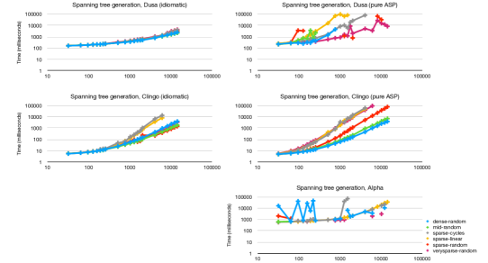
These programs were tested on a group of graphs with different features. The test graphs vary primarily in their number of edges and span three scales, growing by steps of 32 to 256, then by steps of 256 to 2048, then by steps of 2048 to 14336. Results are shown in Figure 11 (the left-hand side graphs are just a log-log plot of Figure 9).

Idiomatic Dusa is the clear winner here for overall consistency, exhibiting slow growth relative to the number of edges that seems to essentially match the linear prediction of the cost semantics On the majority of types, Dusa is outperformed by an idiomatic Clingo ASP program that replaces the four ”Exactly one root” rules with the single rule 1 {root(X) : edge(X,Y)} 1.

The right side of Figure 11 shows a “fair fight,” running the program in Figure 10 on in Dusa, Clingo, and Alpha. Clingo is the most consistent, but Dusa and Alpha outperform it on some sparce graphs, suggesting that Clingo’s performance issues are connected to the ground-then-solve methodology.

B.2.2. Appointing canonical representatives

edge(Y,X) :- edge(X,Y).

% Any node can be a rep
{representative(X,X)} :-
    node(X).

% Connected nodes have same rep
representative(Y,Rep) :-
    edge(X,Y),
    representative(X,Rep).

% Representatives must be unique
:- representative(X,R1),
    representative(X,R2), R1 != R2.

% Every node has a rep
hasRep(X) :-
   representative(X,_).

:- node(X), not hasRep(X).
edge Y X :- edge X Y.

# Any node can be a rep
representative X X is { tt, ff } :-
    node X.

# Connected nodes have same rep
representative X Rep is tt :-
    edge X Y,
    representative Y Rep is tt.

# Representatives must be unique
#forbid representative X R1 is tt,
    representative X R2 is tt, R1 != R2.

# Every node has a rep
hasRep X is tt :-
    representative X _ is tt.
hasRep X is? ff :- node X.
#forbid node X, hasRep X is ff.
Figure 12. Canonical representative identification in ASP, and “automatic” translation to Dusa.

The idiomatic finite-choice logic programming approach to appointing canonical representatives for connected components of an undirected graph is shown in Figure 3 in Section 4.2. An ASP version of this program, and the “automatic” translation of this program to a finite-choice logic program, is shown in Figure 12.

Refer to caption
Figure 13. Canonical representative identification: performance of Dusa, Clingo, and Alpha on graphs with different features. The X-axis is the number of edges in the input graph, the Y-axis is running time in milliseconds. All data points are the median of three runs requesting a single solution, discarding timeouts.

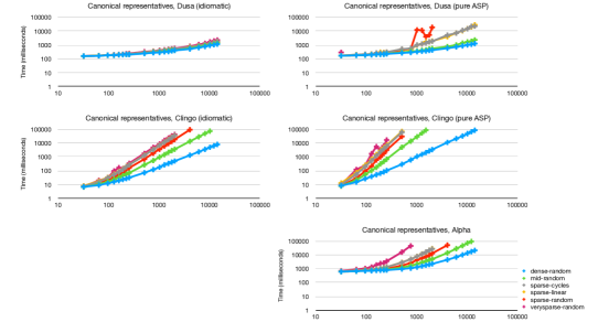
As in the previous section, it’s possible to get a shorter and more performant Clingo program by using Clingo-supported extensions to the ASP language: in this case, the last three ASP rules in Figure 12 can be replaced by the single Clingo rule

:- node(X), not 1{representative(X,R) : node(R)}1. In this case, however,

idiomatic Dusa the clear winner in all cases. Both Dusa and Alpha outperform Clingo in come cases on the same ASP program. This is not terribly surprising: in a graph with $v$ nodes, Clingo’s grounder is almost unavoidably going to require $O(v^{3})$ groundings of the key rule that requires connected nodes to have the same rep. It is a bit more surprising that, on all but the sparsest graphs, Dusa generally outperformed Alpha despite the implementation exerting almost no control over backtracking.

B.3. Examples ill-suited to the current Dusa implementation

In this section we compare Dusa to Clingo on two problems where we expect Dusa to perform poorly, because they require brute-force search. These represent low-hanging fruit for optimization of Dusa.

B.3.1. N-queens

The N-queens problem is a classic of algorithmic expressiveness. The problem is to place N queens on an N-by-N chessboard such that no two queens can immediately attack each other. We used the 2014 notes “Basic modeling and ASP and more via the n-Queens puzzle” by Torsten Schaub as a guide for the ASP implementations.333https://www.cs.uni-potsdam.de/~torsten/Potassco/Videos/BasicModeling/modeling.pdf Schaub’s solutions are not pure ASP, so we can’t just turn a crank to translate them to Dusa. Instead, we’ll consider a spectrum of two different Clingo solutions, and three different finite-choice logic programming solutions.

Basic Clingo implementation
{ queen(1..n,1..n) }.

 :- not { queen(I,J) } == n.
 :- queen(I,J), queen(I,JJ), J != JJ.
 :- queen(I,J), queen(II,J), I != II.
 :- queen(I,J), queen(II,JJ), (I,J) != (II,JJ), I-J == II-JJ.
 :- queen(I,J), queen(II,JJ), (I,J) != (II,JJ), I+J == II+JJ.
Figure 14. Basic N-queens program in Clingo’s dialect of answer-set programming.

The most basic ASP implementation of N-Queens is given in Figure 14. Reading the rules in order, they express:

  • Each spot in an N-by-N grid can have a queen or not.

  • There must be exactly N queens.

  • No two queens can share the same column.

  • No two queens can share the same row.

  • No two queens can share the same diagonal (in either direction).

This is a “sculptural” approach to answer set programming where the problem is explained in the most general terms, and then constraints are used to carve out out parts of the problem space that are not wanted.

The notation { queen(I, J) } == n in Figure 14 counts the number of occurrences of the queen predicate. Creating an analogue in finite-choice logic programming would probably require a form of stratified negation as discussed in Section 7.2. Our implementation doesn’t support range notation 1..n, but this is simple to emulate as a relation dim that contains all the numbers from 1 to N. This is shown in Figure 15.

#builtin INT_MINUS minus
#builtin INT_PLUS plus
dim N :- size is N.
dim (minus N 1) :- dim N, N != 1.
# Expands to: dim Nminus1 :- dim N, N != 1, minus N 1 is Nminus1.
Figure 15. Dusa declarations for using arithmetic and making a dim relation containing the numbers from 1 to declared size, inclusive.
On externally-computed predicates in Dusa

Figure 15 also demonstrates the use of integers and integer operations in Dusa, which is supported by our implementation and our theory. The theory of finite-choice logic programming supports treating externally-computed predicates as infinite relations. The most fundamental such relations are equality and inequality on terms and comparison of numbers, and these have built-in syntax in the Dusa implementation. Premises like “4 > X”, “N != 1”, or “P == pair X Y” can be thought of as referring to infinite relations: in the language of the paper, we would write 𝑔𝑡(𝟦,x)𝑔𝑡4𝑥{{{\color[rgb]{.5,.5,.5}\definecolor[named]{pgfstrokecolor}{rgb}{.5,.5,.5}\pgfsys@color@gray@stroke{.5}\pgfsys@color@gray@fill{.5}\mathit{gt}}({\color[rgb]{0,.5,.5}\definecolor[named]{pgfstrokecolor}{rgb}{0,.5,.5}\mathsf{4}},x)}}, 𝑛𝑒𝑞(n,𝟣)𝑛𝑒𝑞𝑛1{{{\color[rgb]{.5,.5,.5}\definecolor[named]{pgfstrokecolor}{rgb}{.5,.5,.5}\pgfsys@color@gray@stroke{.5}\pgfsys@color@gray@fill{.5}\mathit{neq}}(n,{\color[rgb]{0,.5,.5}\definecolor[named]{pgfstrokecolor}{rgb}{0,.5,.5}\mathsf{1}})}}, or 𝑒𝑞(p,𝗉𝖺𝗂𝗋(x,y))𝑒𝑞𝑝𝗉𝖺𝗂𝗋𝑥𝑦{{{\color[rgb]{.5,.5,.5}\definecolor[named]{pgfstrokecolor}{rgb}{.5,.5,.5}\pgfsys@color@gray@stroke{.5}\pgfsys@color@gray@fill{.5}\mathit{eq}}(p,{\color[rgb]{0,.5,.5}\definecolor[named]{pgfstrokecolor}{rgb}{0,.5,.5}\mathsf{pair}}(x,y))}}, respectively.

Our theory and implementation are able to handle operating on infinite relations as long as:

  1. (1)

    Infinite relations are never present in the conclusion of a rule, and

  2. (2)

    It is tractable to find all the substitutions that satisfy a premise.

In the implementation, syntactic checks prevent us from writing rules like p(x)𝑔𝑡(𝟦,x)𝑝𝑥𝑔𝑡4𝑥{{{\color[rgb]{.5,.5,.5}\definecolor[named]{pgfstrokecolor}{rgb}{.5,.5,.5}\pgfsys@color@gray@stroke{.5}\pgfsys@color@gray@fill{.5}\mathit{p}}(x)}}\leftarrow{{{\color[rgb]{.5,.5,.5}\definecolor[named]{pgfstrokecolor}{rgb}{.5,.5,.5}\pgfsys@color@gray@stroke{.5}\pgfsys@color@gray@fill{.5}\mathit{gt}}({\color[rgb]{0,.5,.5}\definecolor[named]{pgfstrokecolor}{rgb}{0,.5,.5}\mathsf{4}},x)}} or p(x,y)𝑒𝑞(x,y)𝑝𝑥𝑦𝑒𝑞𝑥𝑦{{{\color[rgb]{.5,.5,.5}\definecolor[named]{pgfstrokecolor}{rgb}{.5,.5,.5}\pgfsys@color@gray@stroke{.5}\pgfsys@color@gray@fill{.5}\mathit{p}}(x,y)}}\leftarrow{{{\color[rgb]{.5,.5,.5}\definecolor[named]{pgfstrokecolor}{rgb}{.5,.5,.5}\pgfsys@color@gray@stroke{.5}\pgfsys@color@gray@fill{.5}\mathit{eq}}(x,y)}} that might have infinitely many satisfying substitutions.

Additional built-in operations like addition and subtraction are included with #builtin directives. These are also treated like infinite relations. Figure 15 also demonstrates an additional language convenience that we picked up from LogiQL (Aref et al., 2015): the language supports treating built-in relations with functional dependencies like functions, so we can write dim (minus N 1) instead of needing to write dim Nminus1 and including minus N 1 is Nminus1 as an additional premise.

location N is? (tup X Y) :-
  dim N, dim X, dim Y.


#forbid
  location N is (tup X _),
  location M is (tup X _),
  N != M.
#forbid
  location N is (tup _ Y),
  location M is (tup _ Y),
  N != M.
#forbid
  location N is (tup X1 Y1),
  location M is (tup X2 Y2),
  N != M,
  minus X1 Y1 == minus X2 Y2.
#forbid
  location N is (tup X1 Y1),
  location M is (tup X2 Y2),
  N != M,
  plus X1 Y1 == plus X2 Y2.
col N is { X? } :-
  dim N, dim X.
row N is { Y? } :-
  dim N, dim Y.

#forbid
  col N is X, col M is X,
  N != M.

#forbid
  row N is Y, row M is Y,
  N != M.

#forbid
  row N is X1, col N is Y1,
  row M is X2, col M is Y2,
  N != M,
  minus X1 Y1 == minus X2 Y2.
#forbid
  row N is X1, col N is Y1,
  row M is X2, col M is Y2,
  N != M,
  plus X1 Y1 == plus X2 Y2.


rowFor X is { Y? } :-
  dim X, dim Y.


colFor Y is X :-
  rowFor X is Y.


posDiag (plus X Y)
  is (tuple X Y) :-
  rowFor X is Y.


negDiag (minus X Y)
  is (tuple X Y) :-
  rowFor X is Y.


Figure 16. Three different implementations of N-Queens in Dusa.
N-queens in Dusa

In order to adapt the N-queens problem to finite-choice logic programming, we need a way to ensure that there will be exactly N queens without Clingo’s #count aggregates used in Figure 14. The first program in Figure 16 is the most sculptural: we number each of the N queens and assign a unique coordinate pair to each queen. Our cost semantics suggests that the first rule in this program generates a complexity of $O(n^{3})$ for $n$ queens, and this observation also suggests a slight improvement. The middle program in Figure 16 is a rewrite of the first one where we switch to sixth normal form (as the literature on LogiQL suggests we should prefer (Aref et al., 2015)). Our cost semantics predicts more manageable behavior, quadratic instead of cubic, for this middle program. Despite the fact that this effect is dwarfed by exponential backtracking, the intuition it provides seems good: the middle program performs slightly better than the left program when we test performance.

If we think a bit about the problem, we can avoid the use of #forbid constraints entirely, as shown in the third column of Figure 16. Each column is labeled by an $x$ coordinate, and each row is labeled by a $y$ coordinate, and there is a functional dependency in both directions: each row has a queen in one column, and each column has a queen in one row. This is expressed by the first two rules in the rightmost program. Furthermore, we can assign every cell’s coordinates to a unique numbered diagonal by adding the coordinates (for the diagonals that go up and to the right) or subtracting the coordinates (for the diagonals that go down and to the right). The third and fourth rules in the third program use functional dependencies to invalidate any assignment that places two queens on the same diagonal.

Better Clingo implementation

{ queen(I,1..n) } == 1 :- I = 1..n.
{ queen(1..n,J) } == 1 :- J = 1..n.

 :- { queen(D-J,J) } >= 2, D = 2..2*n.
 :- { queen(D+J,J) } >= 2, D = 1-n..n-1.
Figure 17. More efficient N-queens implementation in Clingo.

The Dusa program we worked our way towards in the previous section is fundamentally using the same ideas as one of Torsten Schaub’s improved Clingo programs, shown in Figure 17. Each of the four rules in Schaub’s more efficient Clingo program corresponds loosely with one of the four rules in our final Dusa program in Figure 16, but Schaub’s version uses Clingo’s counting constraints to enforce the at-most-one-queen-per-diagonal property that is enforced by functional dependencies in Dusa.

Performance
Refer to caption
Figure 18. Performance of the previous five implementations of the N-queens problem in Dusa and Clingo. All data points are the median of three runs requesting 10 different solutions, discarding timeouts.

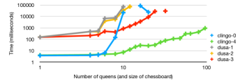
The performance of the two Clingo programs and three Dusa programs from this section is shown in Figure 18 with the problem size scaling from 1 to 100 queens. The first Clingo program scales quite badly and starts hitting the 100-second timeout in at least some runs starting at 12 queens, whereas the optimized Clingo program in Figure 17 is far and away the best. The three successive Dusa programs fall in the middle: the third program from Figure 16 is the best but starts to encounter timeouts at 28 queens.

B.3.2. Map-generation speedrun

dim(1..W) :- width(W).


{ solid(X,Y) :dim(X) :dim(Y) }.


start(1,1).
finish(W,W) :- width(W).
step(0,-1).
step(0,1).
step(1,0).
step(-1,0).

reachable(X,Y) :-
    start(X,Y),
    solid(X,Y).
reachable(NX,NY) :-
    reachable(X,Y),
    step(DX,DY),
    NX = X + DX,
    NY = Y + DY,
    solid(NX,NY).

complete :- finish(X,Y),
    reachable(X,Y).
:- not complete.

at(X,Y, 0) :-
    start(X,Y),
    solid(X,Y).
at(NX,NY, T+1) :-
    at(X,Y,T),
    length(Len),
    T < Len,
    step(DX,DY),
    NX = X + DX,
    NY = Y + DY,
    solid(NX,NY).

speedrun :- finish(X,Y), at(X,Y,T).
:- speedrun.
#builtin INT_PLUS plus
#builtin INT_MINUS minus

dim Width :- width is Width.
dim (minus N 1) :- dim N, N != 1.

solid X Y is { tt, ff } :-
    dim X, dim Y.

start 1 1.
finish W W :- width is W.
step 0 -1.
step 0 1.
step 1 0.
step -1 0.

reachable X Y :-
    start X Y,
    solid X Y is tt.
reachable NX NY :-
    reachable X Y,
    step DX DY,
    NX == plus X DX,
    NY == plus Y DY,
    solid NX NY is tt.

#demand finish X Y,
    reachable X Y.


at X Y 0 :-
    start X Y,
    solid X Y is tt.
at NX NY (plus T 1) :-
    at X Y T,
    length is Len,
    T < Len,
    step DX DY,
    NX == plus X DX,
    NY == plus Y DY,
    solid NX NY is tt.

speedrun :- finish X Y, at X Y _.
#forbid speedrun.
Figure 19. Adam Smith’s Map Generation Speedrun in ASP, and Dusa translation.

Adam Smith’s blog post “A Map Generation Speedrun with Answer Set Programming” is a beautiful example of the sculptural approach to ASP.444https://eis-blog.soe.ucsc.edu/2011/10/map-generation-speedrun/ On a tile grid, we stipulate that every tile can be solid or liquid, and we request maps where only a circuitous route can reach the bottom-right side of the map from the upper-right side.

Figure 19 shows that ASP’s expressiveness translates well into finite-choice logic programming, as the fundamental choice (is a tile land or sea?) is naturally expressed as a closed choice rule. As with the previous example, though, the current Dusa implementation is not well suited to support sculptural specifications.

Refer to caption
Figure 20. Map generation: performance of Dusa, Clingo, and Alpha on different-sized grids. All data points are the median of three runs requesting five different maps where the shortest path from upper-left to lower-right on an $n\times n$ grid was more than $2n+1$, discarding timeouts.

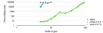
The map generation speedrun is an excellent demonstration of Dusa’s current lack of suitibility for sculptural programming: it times out for all grids larger than $10\times 10$, and times out at least once at every size, including $5\times 5$ grids. Alpha’s relatively poor showing, unable to handle any grids larger than $6\times 6$, was more surprising.

B.4. Alpha benchmarks

Using someone else’s benchmark is a good way to keep yourself honest. We are therefore grateful to Weinzirel (Weinzierl, 2017), who published an easily accessible set of benchmarks for the Alpha implementation of lazy grounding ASP.555http://www.kr.tuwien.ac.at/research/systems/alpha/benchmarks.html Our hypothesis was that this benchmark to be somewhat kind to Dusa, since lazy grounding ASP and the finite-choice logic program translation of ASP share many of the same advantages over the ground-then-solve approach, but would prevent us from just testing Dusa on problems where we expected it to succeed. By in large, the results were similar to our other benchmarks: Dusa performs impressively except on problems that obviously fall back on exponential search.

B.4.1. Ground explosion

p(X1,X2,X3,X4,X5,X6) :-
   select(X1), select(X2), select(X3),
   select(X4), select(X5), select(X6).

select(X) :- dom(X), not nselect(X).
nselect(X) :- dom(X), not select(X).
 :- not nselect(Y), select(X), dom(Y), X != Y.
Figure 21. Ground explosion benchmark.

The ground explosion benchmarks use the program in Figure 21 to trigger pathological behavior in ground-then-solve ASP solvers. For a domain with $n$ elements, a ground-then-solve solver will need to ground $6^{n}$ variants of the first rule, despite the fact that there are only $n+1$ solutions.

Refer to caption
Figure 22. Performance of the Dusa, Clingo, and Alpha solvers on the ground explosion benchmark in Figure 21. All data points are the median of three runs, discarding timeouts.

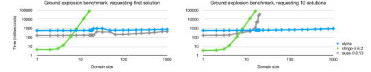
The results from this set of Alpha benchmarks are shown in Figure 22. Dusa was tested with the “automatic” translation of the answer set program. This benchmark shows both the strength of the Dusa implementation and the degree to which backtracking is done naively and inefficiently in Dusa. The first solution is found immediately, matching the asymptotic behavior of the Alpha implementation and improving on constant factors, but enumerating additional solutions is done in a way that results in exponential backtracking, so Dusa is unable to return 10 distinct solutions for most examples. We expect dramatically improving Dusa’s behavior here would be low-hanging fruit.

B.4.2. Graph 5-colorability

chosenColour(N,C) :- node(N), colour(C),
  not notChosenColour(N,C).
notChosenColour(N,C) :- node(N), colour(C),
  not chosenColour(N,C).

:- node(X), not colored(X).
colored(X) :- chosenColour(X,Fv1).

:- node(N), chosenColour(N,C1),
  chosenColour(N,C2), C1!=C2.

colour(red0).
colour(green0).
colour(blue0).
colour(yellow0).
colour(cyan0).

:- node(X), not chosenColour(X,red0),
  not chosenColour(X,blue0),
  not chosenColour(X,yellow0),
  not chosenColour(X,green0),
  not chosenColour(X,cyan0).

:- link(X,Y), node(X), node(Y), X<Y,
  chosenColour(X,C), chosenColour(Y,C).
color N is {
  red,
  green,
  blue,
  yellow,
  cyan
} :- node N.


#forbid link X Y,  X < Y,
  color X is C, color Y is C.
Figure 23. Graph 5-colorability expressed in ASP (left) and finite-choice logic programming (right).

A graph is 5-colorable if each node can be assigned one of five different colors such that no edge connects nodes of the same color. Perhaps there is a dramatically clearer way to express this concept in ASP than the ASP code from the benchmark shown in Figure 23, but it was remarkable how much simpler this is to express in finite-choice logic programming, as shown on the right side of Figure 23.

Refer to caption
Figure 24. Performance of the Dusa, Clingo, and Alpha solvers on 5-colorability benchmark from Figure 23. The Y-axis is running time in milliseconds, and all data points are the average of ten runs on different graphs requesting 10 different solutions each time, discarding timeouts. (The same data points with 50 nodes and 200 edges are present in both graphs.)

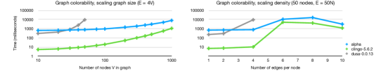
This is essentially a pure search problem, so it’s not surprising that the Dusa implementation performs quite badly. We didn’t bother testing the performance of the finite-choice logic program “automatically” translated from the ASP program in Figure 23, since the idiomatic program already exhibited poor performance.

B.4.3. “Cutedge” benchmark

delete(X,Y) :- edge(X,Y), not keep(X,Y).
keep(X,Y) :- edge(X,Y), delete(X1,Y1), X1 != X.
keep(X,Y) :- edge(X,Y), delete(X1,Y1), Y1 != Y.
reachable(X,Y) :- keep(X,Y).
reachable(X,Y) :- special(Y),reachable(X,Z),reachable(Z,Y).
Figure 25. “Cutedge” benchmark.

The “cutedge” benchmarks shown in Figure 25 remove an arbitrary edge from a graph and then calculate reachability from one endpoint of the removed edge and another specially designated node. The benchmark seems to be intended to force bad performance on ground-then-solve approaches without being as obviously unfair as the ground explosion benchmark. The “automatic” translation of this ASP program to a finite-choice logic program was used in Dusa. Figure 26 shows the very similar performance of Dusa and Alpha. Clingo is not shown, as it was only able to handle the 100 node cases without timeouts, though it managed to return results for 1 of the 10 runs 300-node graphs with 10% edge density.

Refer to caption
Figure 26. Performance of the Dusa and Alpha solvers on the “cutedge” benchmark from Figure 25 on random graphs with different edge probabilities. All data points are the average of ten runs requesting 10 different solutions, discarding timeouts.

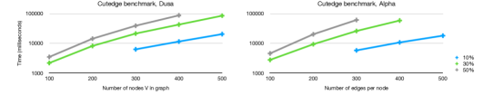
B.4.4. Graph reachability benchmark

The graph reachability benchmark (Figure 27) is included for completeness, but the test cases weren’t particularly interesting. It would be more interesting to rerun this test on the graphs used to test the spanning tree and canonical representative programs here order to tease apart different asymptotic behaviors.

reachable(X, Y) :- edge(X, Y).
reachable(S, Y) :- start(S), reachable(S, X), reachable(X, Y).
Figure 27. Graph reachability.
Instance size Dusa Clingo Alpha
1000/4 0.4 0.05 0.8
1000/8 0.5 0.1 0.9
10000/2 1.9 1.1 1.2
10000/4 3.6 2.3 1.6
10000/8 2.3 5.1 2.1
Figure 28. Performance of the Dusa, Clingo, and Alpha solvers on the graph reachability program from Figure 27. Instance size is number of nodes / number of edges per node, running time in seconds, and all data points are the average of ten runs on different graphs requesting 10 different solutions each time (though there is in fact only one unique solution in each case).