State Space Models are Comparable to Transformers
in Estimating Functions with Dynamic Smoothness

Abstract

Deep neural networks based on state space models (SSMs) are attracting much attention in sequence modeling since their computational cost is significantly smaller than that of Transformers. While the capabilities of SSMs have been primarily investigated through experimental comparisons, theoretical understanding of SSMs is still limited. In particular, there is a lack of statistical and quantitative evaluation of whether SSM can replace Transformers. In this paper, we theoretically explore in which tasks SSMs can be alternatives of Transformers from the perspective of estimating sequence-to-sequence functions. We consider the setting where the target function has direction-dependent smoothness and prove that SSMs can estimate such functions with the same convergence rate as Transformers. Additionally, we prove that SSMs can estimate the target function, even if the smoothness changes depending on the input sequence, as well as Transformers. Our results show the possibility that SSMs can replace Transformers when estimating the functions in certain classes that appear in practice.

1 Introduction

Foundation models based on Transformers have achieved remarkable success in various sequence modeling tasks such as natural language processing (Vaswani et al., 2017), computer vision (Dosovitskiy et al., 2020), and speech recognition (Radford et al., 2023). The superior performance of Transformers is attributed to the self-attention mechanism, which enables the model to aggregate the information from the input sequence.

In contrast to its success, self-attention mechanism has a potential problem that it requires a large amount of computation and memory. To deal with this issue, many studies have been attempted to develop efficient models that can replace Transformers. Among them, Structured State Space Models (SSMs) have garnered considerable interest recently. One advantage of SSMs is that the output can be computed with a significantly small time using convolution via FFT algorithm or recursive computation. Based on the original SSMs, many improvements have been proposed, such as HiPPO-based intialization (Gu et al., 2021) and architectures using gated convolutions (Fu et al., 2022, Poli et al., 2023).

Networks based on SSMs have accomplished high performance in various applications such as gene analysis (Nguyen et al., 2024), audio generation (Goel et al., 2022) and speech recognition (Saon et al., 2023). On the other hand, some of the recent studies pointed out the limitations of SSMs, especially for their abilities to solve tasks. For example, Merrill et al. (2024) show that SSMs cannot solve sequential problems from the view of computational complexity theory. Additionally, Gu and Dao (2023) pointed out that SSMs are less effective for the tasks to handle discrete and information-dense data such as language processing. Therefore, it is still unclear in what situation we can replace Transformers with SSMs.

Recently, some studies have theoretically investigated the abilities of SSMs. For instance, Wang and Xue (2024) show that SSMs are universal approximators for continuous sequence-to-sequence functions. Additionally, Massaroli et al. (2024) constructed the parameters of SSMs to solve the task called associated recall. Moreover, Cirone et al. (2024) studied the abilities of SSMs using rough path theory. However, they mainly focus on the expressive power of SSMs and do not provide statistical understanding. Furthermore, quantitative evaluations to compare SSMs and Transformers is limited.

Leaving aside SSMs, many studies have investigated the abilities of deep neural networks to estimate functions. Some of them analyze the estimation abilities of fully connected neural networks (FNNs) with the assumption that the target function is in certain function classes (Schmidt-Hieber, 2020, Suzuki, 2018) or have a specific smoothness structure (Suzuki and Nitanda, 2021). Moreover, Nakada and Imaizumi (2020) and Chen et al. (2022) consider the setting that the data distribution has a low-dimensional structure. Additionally, Okumoto and Suzuki (2021) studied convolutional neural networks (CNNs) and showed that CNNs can estimate the functions that have smoothness structures with the minimax optimal rate even if the input is infinite-dimensional. As for the Transformers, Takakura and Suzuki (2023) showed that Transformers can estimate the functions with infinite-dimensional input as well as CNNs. Additionally, they showed that Transformers can estimate the functions whose smoothness structure changes depending on the input.

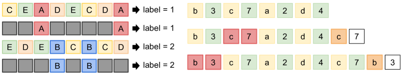
Figure 1.1: Conceptual illustrations of the abilities of SSMs. Left: This represents the classification task in which the existence of the token “A” or “B” is important. We prove that SSMs can extract such tokens, even if the position of the important token is different for each input. Right: This illustrate the task to predict the next token in the sequence. In this task, models have to output the token associated with the last token. We also prove that SSMs can solve such tasks, i.e., SSMs can extract appropriate tokens even if the position of essential tokens are different for each token in the same sequence.

Our contributions.

In this paper, we explore the abilities of SSMs with gated convolution to replace Transformers from the perspective of statistical learning theory. More specifically, we investigate the estimation ability of SSMs for the function classes called $\gamma$-smooth and piecewise $\gamma$-smooth. For the function in these classes, Takakura and Suzuki (2023) showed that Transformers can estimate them effectively. We prove that SSMs can also estimate those functions with the same convergence rate as Transformers, and show that SSMs can replace Transformers when estimating those functions.

The essential point of the two function classes above is that they have smoothness structures. As for $\gamma$-smooth functions, the smoothness of the function is the same for all input sequences, i.e., the important features to extract are fixed. On the other hand, piecewise $\gamma$-smooth functions have different smoothness depending on the input. This function class characterizes the ability of Transformers and SSMs to extract important features dynamically. In addition to the settings considered in Takakura and Suzuki (2023), we also consider the functions whose smoothness structure also changes depending on the position output token. This setting is inspired by the ability of Transformers to solve the task called associative recall (Ba et al., 2016). We show that SSMs can also replace Transformers in this setting. See Figure 1.1 for the conceptual illustrations of those function classes.

The contributions of this paper are summarized as follows:

1. We theoretically investigate the estimation ability of SSMs with gated convolutions for $\gamma$-smooth functions and piecewise $\gamma$-smooth functions. We show that SSMs can achieve the same estimation error as Transformers, which implies that SSMs may be alternative to Transformers in terms of estimating functions in those classes.

2. Inspired by recent research on the abilities of Transformers, we define function classes that are extensions of the piecewise $\gamma$-smooth function class. Then, we prove that SSMs can also attain the similar estimation error for those classes.

Other related works.

The function classes with piecewise smoothness are also considered in Petersen and Voigtlaender (2018) and Imaizumi and Fukumizu (2019). They do not consider anisotropic smoothness or the sequence-to-sequence functions, while we consider such situations.

One of the other directions to investigate the abilities of SSMs is to utilize the control theory, like Alonso et al. (2024). Instead of focusing on the statistical aspect, they mainly provide a comprehensive understanding of existing SSMs.

Gu and Dao (2023) proposed an SSM-based architecture called Mamba, whose filter is controlled by the input. While convolution with FFT algorithms cannot be used for Mamba, they proposed a hardware-aware efficient implementation. In this paper, we do not focus on the setting that filters are controlled by the input, and we consider SSMs with gated convolution with data-independent filters.

Notations.

For $l\in\mathbb{N}$, let $[l]$ be the set $\quantity{1,\dots,l}$ and for $l,r\in\mathbb{Z}~{}(l\leq r)$, let $[l:r]$ be the set $\quantity{l,\dots,r}$. For a set $S\subseteq\mathbb{R}$ and $d\in\mathbb{N}$, let $S^{d\times\infty}\coloneqq\quantity{[\dots,s_{-2},s_{-1},s_{0}]\mid s_{i}\in S^{d}}$. For $F:\Omega\to\mathbb{R}^{l}$, let $\norm{F}_{\infty}:=\sup_{X\in\Omega}\norm{F(X)}_{\infty}$. For the probability measure $P_{X}$ on $\Omega$ and $p>0$, the norm $\norm{\cdot}_{p,P_{X}}$ is defined by $\norm{f}_{p,P_{X}}=\left(\int_{\Omega}\norm{f(X)}_{p}^{p}\differential{P_{X}}\right)^{1/p}.$ For a matrix $A$, let $\norm{A}_{0}=\absolutevalue{\quantity{(i,j)\mid A_{ij}\neq 0}}$. For $F\colon\mathbb{R}^{d\times\infty}\to\mathbb{R}^{1\times\infty}$, we denote $F=(F_{j})_{j=-\infty}^{\infty}$ with $F_{j}\colon[0,1]^{d\times\infty}\to\mathbb{R}$.

2 Problem Settings

In this paper, we consider a non-parametric regression problem where the input is infinite-dimensional. More concretely, we suppose that the input $X\coloneqq\quantity[x_{i}]_{i=-\infty}^{0}\in\mathbb{R}^{d\times\infty}$ is a sequence of $d$-dimensional tokens. Let $P_{X}$ be a probability measure on $([0,1]^{d\times\infty},\mathcal{B}([0,1]^{d\times\infty}))$, and denote $\Omega\coloneqq\operatorname{\operatorname{supp}}(P_{X})$. We assume that $P_{X}$ is shift-invariant, i.e., for any $i\in\mathbb{Z}$ and $B\in\mathcal{B}([0,1]^{d\times\infty})$, it holds that $P_{X}(B)=P_{X}(\quantity{\Sigma_{i}(X)\mid X\in B})$ for any $i\in\mathbb{N}$, where $\Sigma_{j}$ is the shift operator $\Sigma_{j}\colon\mathbb{R}^{d\times\infty}\to\mathbb{R}^{d\times\infty}$ defined by $(\Sigma_{j}(X))_{i}=x_{i-j}$ for $X=[x_{j}]_{j=-\infty}^{0}\in\mathbb{R}^{d\times\infty}$.

We consider the setting where the output is also infinite-dimensional. As same as the usual nonparametric regression setting, suppose that we observe $n$ i.i.d. inputs $X^{(i)}\sim P_{X}~{}(i=1,\ldots,n)$ and the corresponding outputs $Y^{(i)}\in\mathbb{R}^{1\times\infty}$ generated by $Y^{(i)}=F^{\circ}(X^{(i)})+\xi^{(i)}$, where $\xi^{(i)}\in\mathbb{R}^{d\times\infty}$ is the i.i.d. noise generated from $\mathcal{N}(0,\sigma^{2})~{}(\sigma>0)$. We further assume that $\quantity{\xi^{(i)}}_{i=1}^{n}$ is independent of the inputs $\quantity{X^{(i)}}_{i=1}^{n}$.

Given the pairs of inputs and outputs $\quantity{(X^{(i)},Y^{(i)})}_{i=1}^{n}$, we obtain the estimator $\hat{F}$ of the target function $F$ through empirical risk minimization:

$$\hat{F}=\arg\min_{F\in\mathcal{S}}\frac{1}{n}\sum_{i=1}^{n}\sum_{j=l}^{r}\quantity(Y^{(i)}-F^{\circ}(X^{(i)}))^{2},$$

where $\mathcal{S}$ is supposed to be the class of networks that we define in the next section. To measure the statistical performance of the estimator $\hat{F}$, we utilize mean squared error (MSE) defined by

$$R_{l,r}(\hat{F},F^{\circ})=\frac{1}{l-r+1}\sum_{j=l}^{r}\mathbb{E}\quantity[\norm{\hat{F}_{j}(X)-F_{j}^{\circ}(X)}_{2,P_{X}}^{2}],$$

where the expectation is taken for $\quantity{\xi^{(i)}}_{i=1}^{n}$. Note that we consider the average error over the finite segment $[l:r]$ to avoid the technical difficulty of infinite-dimensionality. However, the estimation error analysis in Section 5 is independent of the choice of $l$ and $r$.

Similar to the setting of Takakura and Suzuki (2023), we assume that target function is shift equivariant. That is, we impose that the target function $F\colon\mathbb{R}^{d\times\infty}\to\mathbb{R}^{d\times\infty}$ satisfies $F(\Sigma_{j}(X))=\Sigma_{j}(F(X))$ for any $j\in\mathbb{N}$. This is a natural assumption in various applications such as language processing, audio processing, and time-series analysis. Additionally, we assume that the target function $F$ is included in a certain function classes defined in the remainings of this section.

2.1 $\gamma$-smooth function class

Here, we introduce the $\gamma$-smooth function class, which was first proposed by Okumoto and Suzuki (2021). First of all, for $r\in\mathbb{Z}_{0}^{d\times\infty}$, we define $\psi_{r_{ij}}:[0,1]\to\mathbb{R}$ by

$$\psi_{r_{ij}}(x)\coloneqq\begin{cases}\sqrt{2}\cos(2\pi\absolutevalue{r_{ij}}x)&\quad(r_{ij}<0),\\ 1&\quad(r_{ij}=0),\\ \sqrt{2}\sin(2\pi\absolutevalue{r_{ij}}x)&\quad(r_{ij}>0),\end{cases}$$

and $\psi_{r}:[0,1]^{d\times\infty}\to\mathbb{R}$ by $\psi_{r}(X)=\prod_{i=1}\prod_{j=1}\psi_{r_{ij}}(X_{ij})$. Then, $\quantity{\psi_{r}}_{r\in\mathbb{Z}_{0}^{d\times\infty}}$ forms a complete orthonormal system of $L^{2}([0,1]^{d\times\infty})$, Therefore, any $f\in L^{2}([0,1]^{d\times\infty})$ can be expanded as $f=\sum_{r\in\mathbb{Z}_{0}^{d\times\infty}}\expectationvalue{f,\psi_{r}}\psi_{r}$. For $s\in\mathbb{N}_{0}^{d\times\infty}$, we define

$$\delta_{s}(f)\coloneqq\sum_{r\in\mathbb{Z}_{0}^{d\times\infty},\lfloor 2^{{s_{ij}-1}}\rfloor\leq r_{ij}<2^{s_{ij}}}\expectationvalue{f,\psi_{r}}\psi_{r}.$$

Then, we define the $\gamma$-smooth function class as follows.

Definition 2.1 ($\gamma$-smooth function class).

For a given $\gamma:\mathbb{N}_{0}^{d\times\infty}\to\mathbb{R}$ which is monotonically non-decreasing with respect to each coordinate and $p\geq 2,\theta\geq 1$, we define the $\gamma$-smooth function space as follows:

$$\mathcal{F}_{p,\theta}^{\gamma}([0,1]^{d\times\infty})\coloneqq\quantity{f\in L^{2}([0,1]^{d\times\infty})\mid\norm{f}_{\mathcal{F}_{p,\theta}^{\gamma}}<\infty},$$

where the norm $\norm{f}_{\mathcal{F}_{p,\theta}^{\gamma}}$ is defined as $\norm{f}_{\mathcal{F}_{p,\theta}^{\gamma}}\coloneqq\quantity(\sum_{s\in\mathbb{N}_{0}^{d\times\infty}}2^{\theta\gamma(s)}\norm{\delta_{s}(f)}_{p,P_{X}}^{\theta})^{1/\theta}$. We also define the finite dimensional version of $\gamma$-smooth function space $\mathcal{F}_{p,\theta}^{\gamma}([0,1]^{d\times l})$ for $l\in\mathbb{N}$ in the same way.

Note that $\delta_{s}(f)$ can be seen as the frequency component of $f$ with frequency $\absolutevalue{r_{ij}}\sim 2^{s_{ij}}$ toward each coordinate. Therefore, we can interpret that $\gamma$ controls the amplitude of each frequency component through weighting the term $\norm{\delta_{s}(f)}_{p,P_{X}}$ in the norm. In other words, if $\gamma(s)$ is larger, the norm of frequency component $\delta_{s}(f)$ is smaller.

As a special case of $\gamma$, we consider the following two types of smoothness:

Definition 2.2 (Mixed and anisotropic smoothness).

For $a\in\mathbb{R}_{>0}^{d\times\infty}$, mixed smoothness and anisotropic smoothness is defined as follows:

$$\begin{array}[]{ll}\text{{(Mixed smoothness)}}&\quad\gamma(s)=\expectationvalue{a,s},\\ \vspace{-2mm}&\\ \text{{(Anisotropic smoothness)}}&\quad\gamma(s)=\max\quantity{a_{ij}s_{ij}\mid i\in[d],j\in\mathbb{Z}}.\end{array}$$

For each $i\in[d],j\in\mathbb{Z}$, the parameter $a_{ij}$ can be viewed as the smoothness for the coordinate $X_{ij}$. When $a_{ij}$ is large, $\gamma(s)$ with $s_{ij}\neq 0$ increases and the frequency component $\delta_{s}(f)$ with $s_{ij}\neq 0$ becomes smaller. In contrast, small $a_{ij}$ implies that the function is not smooth towards the coordinate $(i,j)$, which implies that $X_{ij}$ is an important feature.

The function class $\mathcal{F}_{p,\theta}^{\gamma}([0,1]^{d\times\infty})$ can be seen as extension of some famous function spaces to the infinite-dimensional setting. Indeed, if $P_{X}$ is uniform distribution on $[0,1]^{1\times l}$ and $p<\infty$, then $\mathcal{F}_{p,\theta}^{\gamma}([0,1]^{1\times l})$ with mixed smoothness is equivalent to the mixed-Besov space. Moreover, if $P_{X}$ is uniform distribution, then the anisotropic Sobolev space included in the unit ball of $\mathcal{F}_{2,2}^{\gamma}$ with anisotropic smoothness.

At the close of this subsection, we introduce some notation related to the smoothness parameter $a$. Let $\bar{a}$ be the sequence obtained by sorting $a$ in ascending order. That is, $\bar{a}=[a_{i_{1},j_{1}},\dots,a_{i_{k},j_{k}},\dots]$ satisfies $a_{i_{k},j_{k}}\leq a_{i_{k+1},j_{k+1}}$ for any $k\in\mathbb{N}$. Then, we define weak $l^{\alpha}$-norm for $\alpha>0$ as $\norm{a}_{wl^{\alpha}}:=\sup_{j}j^{\alpha}\bar{a}_{j}^{-1}.$ Additionally, we define $a^{\dagger}=\bar{a}_{1}$ for the mixed smoothness and $a^{\dagger}=\quantity(\sum_{i=1}^{\infty}\bar{a}_{i}^{-1})^{-1}$ for the anisotropic smoothness.

2.2 Piecewise $\gamma$-smooth function class

In this subsection, we describe the piecewise $\gamma$-smooth function class. This was firstly proposed by Takakura and Suzuki (2023) to clarify the advantage of Transformers compared to CNNs. More specifically, they pointed out that Transformers have ability to determine which features to extract depending on the input, while the estimation error analysis for $\gamma$-smooth function class does not reflect such ability. Since piecewise $\gamma$-smooth function has different smoothness depending on the input unlike $\gamma$-smooth function, it is necessary to choose appropriate features to extract when estimating a function in this class.

The rigourous definition of piecewise $\gamma$-smooth function class is given as follows.

Definition 2.3 (Piecewise $\gamma$-smooth function class).

For an index set $\Lambda$, let $\quantity{\Omega_{\lambda}}_{\lambda\in\Lambda}$ be a disjoint partition of $\Omega$. That is, $\quantity{\Omega_{\lambda}}_{\lambda\in\Lambda}$ satisfies $\Omega=\bigcup_{\lambda\in\Lambda}\Omega_{\lambda},~{}\Omega_{\lambda}\cap\Omega_{\lambda^{\prime}}=\emptyset~{}(\lambda\neq\lambda^{\prime}).$ For $V\in\mathbb{N}$ and a set of bijections $\quantity{\pi_{\lambda}}_{\lambda\in\Lambda}$ between $[V+1]$ and $[-V:0]$, define $\Pi_{\lambda}:\mathbb{R}^{d\times[-V:0]}\to\mathbb{R}^{d\times(V+1)}$ and $\Pi:\Omega\to\mathbb{R}^{d\times(V+1)}$ by

$$\Pi_{\lambda}([x_{-V},\dots,x_{0}]) \coloneqq[x_{\pi_{\lambda}(1)},\dots,x_{\pi_{\lambda}(V+1)}],$$

$$\Pi(X) \coloneqq\Pi_{\lambda}(X[-V:0])\quad\text{ if }X\in\Omega_{\lambda}.$$

Then, for $p\geq 2,\theta\geq 1$ and $\gamma:\mathbb{N}_{0}^{d\times\infty}\to\mathbb{R}$, the function class with piecewise $\gamma$-smoothness is defined as follows:

$$\mathcal{P}_{p,\theta}^{\gamma}(\Omega)\coloneqq\quantity{g=f\circ\Pi\mathrel{}\middle|\mathrel{}f\in\mathcal{F}_{p,\theta}^{\gamma}([0,1]^{d\times(V+1)}),\norm{g}_{\mathcal{P}_{p,\theta}^{\gamma}}<\infty},$$

where the norm $\norm{g}_{\mathcal{P}_{p,\theta}^{\gamma}}$ is defined by $\norm{g}_{\mathcal{P}_{p,\theta}^{\gamma}}\coloneqq\quantity(\sum_{s\in\mathbb{N}_{0}^{d\times[-V:0]}}2^{\theta\gamma(s)}\norm{\delta_{s}(f)\circ\Pi}_{p,P_{X}}^{\theta})^{1/\theta}.$

For $g\in\mathcal{P}_{p,\theta}^{\gamma}(\Omega)$ and $X\in\Omega_{\lambda_{1}},Y\in\Omega_{\lambda_{2}}$ with $\lambda_{1}\neq\lambda_{2}$, the smoothness parameter of $g$ at $X$ and $Y$ are different. This means that the coordinates of important features can change depending on the input. Takakura and Suzuki (2023) gives the convergence rate of the estimation error, and show that it almost coincides the rate for $\gamma$-smooth functions. This reveals the ability of Transformers to extract important features depending on the input.

To express how the disjoint partitions $\quantity{\Omega_{\lambda}}_{\lambda\in\Lambda}$ are determined, we introduce the importance function defined as follows.

Definition 2.4 (importance function).

A function $\mu:\Omega\to\mathbb{R}^{\infty}$ is called an importance function for $\quantity{\Omega_{\lambda}}_{\lambda\in\Lambda}$ if $\mu$ satisfies $\Omega_{\lambda}=\{X\in\Omega\mid\mu(X)_{\pi_{\lambda}(1)}>\cdots>\mu(X)_{\pi_{\lambda}(V+1)}\}.$

In simple terms, the paritions $\quantity{\Omega_{\lambda}}_{\lambda\in\Lambda}$ are determined to sort the inputs in descending order of the importance function. As same as Takakura and Suzuki (2023), we assume that an importance function $\mu$ is well-separated, i.e., for some constant $c,\beta>0$, $\mu$ satisfies $\mu(X)_{\pi_{\lambda}(i)}\geq\mu(X)_{\pi_{\lambda}(i+1)}+ci^{-\beta}$ for any $X\in\Omega_{\lambda}$. This implies the probability that $X$ satisfies $\mu(X)_{i}\simeq\mu(X)_{j}~{}(i\neq j)$ is zero. Similar assumption can be found in the literature of statistics such as Hall and Horowitz (2007).

2.3 Function class for the importance function

As for the importance function $\mu$, Takakura and Suzuki (2023) assume that it belongs to $\gamma$-smooth function class. Consequently, the value of importance of a token is unique in the input sequence, and does not change depending on the position of the output token. In order to consider the setting where the importance of tokens can change depending on the output token, in addition to the case where $\mu$ is (i) $\gamma$-smooth, we consider the following case:

(ii) similarity of features: Let $\zeta_{1},\ldots,\zeta_{d^{\prime}}\in\mathcal{F}_{p,\theta}^{\gamma}$, and $v_{j}\coloneqq\quantity[\zeta_{i}(\Sigma_{j}X)]_{i=1}^{d^{\prime}}\in\mathbb{R}^{d^{\prime}}~{}(j\in\mathbb{N})$. Suppose that $\norm{v_{j}}_{2}\leq 1$ for any $j\in\mathbb{N}$. Then, the importance function $\mu$ is can be represented by $\mu(X)=\quantity[-\norm{v_{0}-v_{j}}_{2}]_{j=-\infty}^{0}$ or $\mu(X)=\quantity[v_{0}^{\top}v_{j}]_{j=-\infty}^{0}$.

In this setting, $v_{j}$ intuitively represents the features of the token at the position $j$, and we assume that the importance of a token is controlled by the similarity between the target token and the current token.

The setting (ii) makes it possible for us to consider additional synthetic task. Specifically, the functions in setting (ii) includes the task called associative recall Ba et al. (2016). In this task, the query token has appeared in the past, and the model is required to output the same token that followed it in the previous occurrence, e.g., if the input is “a 2 c 4 b 3 d 1 e 7 c”, the model should output “4”. Additionally, (ii) includes in-context learning with $k$-nearest neighbors algorithm.

Note that the setting (i) includes some important settings such as induction head and selective copying Gu and Dao (2023). Indeed, in those tasks, the absolute position of the important token is fixed.

3 The Definition of State Space Models with Gated Convolution

(Discretized) state space models with input $[u_{t}]_{t=-L}^{0}$, the latent vectors $[x_{t}]_{t=-L}^{0}$ and the output $[y_{t}]_{t=-L}^{0}$ ($u_{t}\in\mathbb{R},x_{t}\in\mathbb{R},y_{t}\in\mathbb{R}$) is represented as follows:

$$x_{t+1}=\mathsf{A}x_{t}+\mathsf{B}u_{t},\quad y_{t}=\mathsf{C}x_{t}+\mathsf{D}u_{t}\quad(t=-L,\ldots,-1),$$

where $\mathsf{A},\mathsf{B},\mathsf{C},\mathsf{D}\in\mathbb{R}$ are the (learnable) parameters. Then, the output $y_{t}$ can be written explicitly as $y_{t}=\sum_{n=0}^{L+t}\left(\mathsf{C}\mathsf{A}^{t-n}\mathsf{B}+\mathsf{D}\delta_{t-n}\right)u_{n}.$ By setting $h_{t}\coloneqq\mathsf{C}\mathsf{A}^{t}\mathsf{B}+\mathsf{D}\delta_{t}$ and $h=[h_{t}]_{t=0}^{L}$, we can rewrite the output as $y_{t}=(h\ast u)_{t}\coloneqq\sum_{n=0}^{L+t}h_{t-n}u_{n}.$ If the filter $[h_{t}]_{t=0}^{L}$ is precomputed, the output can be computed with $O(L\log L)$ time complexity using FFT algorithm, which is much faster than the computation cost of Transformers, $O(L^{2})$.

In this paper, we consider the state space models with gated convolution like H3 (Fu et al., 2022) and Hyena (Poli et al., 2023). State space model with gated convolution is an architecture that consists of the three components: (i) FNN layers, (ii) gated convolution layers, and (iii) an embedding layer.

(i) FNN layer

An FNN with depth $L$ and width $W$ is defined as

$$f(x)\coloneqq(A_{L}\eta(\cdot)+b_{L})\circ\dots\circ(A_{1}x+b_{1}),$$

where $\eta=\mathrm{ReLU}$, and $A_{i}\in\mathbb{R}^{d_{i+1}\times d_{i}},b_{i}\in\mathbb{R}^{d_{i+1}}$ with $\max_{i}d_{i}\leq W$. Then, we define the class of FNN with depth $L$, width $W$, norm bound $B$ and sparsity $S$ by

$$\Psi(L,W,S,B):=\left\{f\mathrel{}\middle|\mathrel{}\max_{i}\quantity{\norm{A_{i}}_{\infty},\norm{b_{i}}_{\infty}}\leq B,~{}\sum_{i=1}^{L}\norm{A_{i}}_{0}+\norm{b_{i}}_{0}\leq S\right\}.$$

(ii) Gated convolution layer

​​​​ Next, we define gated convolution, which is an idea originally proposed by Dauphin et al. (2017). Let $W_{V},W_{Q}\in\mathbb{R}^{D\times D}$ be learnable weights, and $D$ be the embedding dimension. Then, the gated convolution layer $g\colon\mathbb{R}^{|X|}\to\mathbb{R}^{|X|}$ with window size $U$ is defined as

$$g(X)\coloneqq(W^{Q}X)\odot\quantity(H\ast(W^{V}X)),\quad H_{k,j}\coloneqq c_{1,k}\cos\quantity(\frac{2\pi j\cdot a_{1,k}}{U})+c_{2,k}\sin\quantity(\frac{2\pi j\cdot a_{2,k}}{U}),$$

where $H\in\mathbb{R}^{D\times U}$ is a filter controlled by learnable parameters $c_{1},c_{2},a_{1},a_{2}\in\mathbb{R}^{D}$. Note that $\odot\colon\mathbb{R}^{D}\times\mathbb{R}^{D}\to\mathbb{R}^{D}$ is the element-wise product, and $X\ast Y\coloneqq\quantity[X_{i}\ast Y_{i}]_{i=1}^{d}$ for $X=[X_{i}]_{i=1}^{d}\in\mathbb{R}^{d\times\infty},Y=[Y_{i}]_{i=1}^{d}\in\mathbb{R}^{d\times\infty}$. Then, we define the class of gated convolution layer with window size $U$, embedding dimension $D$ and norm constraint $B$ by

$$\mathcal{C}(U,D,B)\coloneqq\quantity{g\mathrel{}\middle|\mathrel{}\max\quantity{\norm{W^{V}}_{\infty},\norm{W^{Q}}_{\infty},\norm{a_{1}}_{\infty},\norm{a_{2}}_{\infty},\norm{c_{1}}_{\infty},\norm{c_{2}}_{\infty}}\leq B}.$$

This setting is basically inspired Hyena, in which neural networks with $\sin$ activation is used as a convolution filter. However, this can be easily extended to the SSMs with gated convolution with ordenary filter $h_{t}=\mathsf{C}\mathsf{A}^{t}\mathsf{B}+\mathsf{D}\delta_{t}$. Indeed, by constructing the parameters in the filter appropriately, we can obtain the same architecture as the gated convolution layer. See Appendix A for the details. Note that we assume the finite window size $U$, as well as Takakura and Suzuki (2023).

(iii) Embedding layer

Finally, we define the embedding layer. For embedding dimension $D$, an embedding layer is defined as

$$\mathrm{Emb}(X)=[E_{1}X_{i}+E_{2}]_{i=-\infty}^{\infty},$$

where $E_{1}\in\mathbb{R}^{D\times d}$ and $E_{2}\in\mathbb{R}^{D}$ are learnable parameters.

Then, the output of the whole network for input $X$ is computed by $f_{M}\circ g_{M}\circ\cdots\circ f_{1}\circ g_{1}\circ\mathrm{Emb}(X)$. Due to the technical convenience to analyze the estimation error, we consider the setting where the output of the network is bounded. For this purpose, we assume that the output above is fed into the function $\mathrm{clip}_{R}$ defined by $\displaystyle\mathrm{clip}_{R}(x)\coloneqq\begin{cases}R&\quad(x>R),\\ x&\quad(-R\leq x\leq R),\\ -R&\quad(x<-R).\end{cases}$ Since $\mathrm{clip}_{R}$ can be implemented by the FNN with depth $1$ and width $2$, such assumption does not far from the practical setting.

Summarizing above, we define the class of data-controlled SSMs by

$$\mathcal{S}(M,U,D,L,W,S,B)\!\coloneqq\!\!\left\{\!\mathrm{clip}_{R}\circ f_{M}\circ g_{M}\circ\cdots\circ f_{1}\circ g_{1}\circ\mathrm{Emb}\!\mathrel{}\middle|\mathrel{}\begin{aligned} &f_{i}\in\Psi(L,W,S,B),\\ &g_{i}\in\mathcal{C}(U,D,B),\\ &\|E_{1}\|_{\infty}\leq B,~{}\|E_{2}\|_{\infty}\leq B.\!\end{aligned}\right\}\!.$$

4 Approximation Ability of SSMs with Gated Convolution

4.1 Approximation of $\gamma$-smooth functions

Now, we establish the approximation ability of $\gamma$-smooth functions via SSMs. First, we state the detailed assumptions on the target function.

Assumption 4.1.

The true function $F^{\circ}$ is shift-equivariant and satisfies $F^{\circ}_{0}\in\mathcal{F}_{p,\theta}^{\gamma}$, where $\gamma$ is mixed or anisotropic smoothness. Suppose that it holds $\norm{F}_{\mathcal{F}_{p,\theta}^{\gamma}}\leq 1$ and $\norm{F^{\circ}_{0}}_{\infty}\leq R$, where $R>0$ is a constant. Additionally, we assume the smoothness parameter $a$ satisfies $\norm{a}_{wl^{\alpha}}\leq 1$ for some $0<\alpha<\infty$ and $a_{ij}=\Omega(\log(\absolutevalue{j}+1))$. Moreover, if $\gamma$ is mixed smoothness, we assume $\bar{a}_{1}<\bar{a}_{2}$.

Remark.

The assumption $\norm{a}_{wl^{\alpha}}\leq 1$ implies that the $j$-th smallest element of smoothness parameter $a$ increases polynomially with respect to $j$, which indicates the sparsity of the important features. Moreover, the assuption $a_{ij}=\Omega(\log(\absolutevalue{j}+1))$ means that the token distant from the current token is less important. Thus, those two assumptions are natural in various applications.

Then, we have the following theorem which shows that the SSM can approximate $\gamma$-smooth functions.

Theorem 4.2.

Suppose that target function $F^{\circ}$ satisfies Assumption 4.1. Then, for any $T>0$, there exists an SSM $F\in\mathcal{S}(M,U,D,L,W,S,B)$ with

$$M=1,\quad\log U\sim T,\quad D\sim T^{1/\alpha},\quad L\sim T,\quad W\sim T^{1/\alpha},$$ (4.1)

$$W^{\prime}\sim T^{1/\alpha}2^{T/a^{\dagger}},\quad S\sim T^{2/\alpha}\max\quantity{T^{2/\alpha},T^{2}}2^{T/a^{\dagger}},\quad\log B\sim T^{1/\alpha},$$

such that $\norm{F-F^{\circ}}_{2,P_{X}}\lesssim 2^{-T}.$

The proof can be found in Appendix D. We can see that, the number of parameters to achieve certain error does not suffer from the infinite dimensionality. This is due to the fact the SSMs use same convolution filter for each tokens, as well as self-attention of Transformers.

4.2 Approximation of piecewise $\gamma$-smooth functions

Next, we show that the SSMs can approximate the piecewise $\gamma$-smooth functions. To this end, we first state the detailed assumptions on the target function.

Assumption 4.3.

The true function $F^{\circ}$ is shift-equivariant and satisfies $F^{\circ}_{0}\in\mathcal{P}_{p,\theta}^{\gamma}$, where $\gamma$ is mixed or anisotropic smoothness, and suppose that $\norm{F^{\circ}_{0}}_{\mathcal{P}_{p,\theta}^{\gamma}}\leq 1$ and $\norm{F^{\circ}_{0}}_{\infty}\leq R$, where $R>0$ is a constant. Additionally, we assume $a_{ij}=\Omega(j^{\alpha})$ and $\norm{a}_{wl^{\alpha}}\leq 1$ for some $0<\alpha<\infty$. Moreover, there exists a importance function $\mu$ of $\mathcal{P}_{p,\theta}^{\gamma}$ that is represented by (i) $\gamma$-smooth condition or (ii) similarity. For case (i), we further assume that $\mu$ satisfies Assumption 4.1.

Remark.

The assumptions on the norm of the smoothness parameter $a$ and the function $F_{0}^{\circ}$ are same as Assumption 4.1. The interpretion for the conditions on the importance function is described in Subsection 2.3. The condition $a_{ij}=\Omega(j^{\alpha})$ indicates that the function is smoother with respect to the token with small importance the tokens are sorted in order of decreasing importance by the map $\Pi$. Note that, unlike the case of Assumption 4.1, the condition $a_{ij}=\Omega(j^{\alpha})$ is imposed on the smoothness of permuted tokens, and $j$ can be different from the original position.

Then, we have the following theorem on the approximation ability of SSMs for piecewise $\gamma$-smooth functions.

Theorem 4.4.

Let $F^{\circ}$ be a function satisfying Assumption 4.3. Then, for any $T>0$, there exists a SSM $\hat{F}\in\mathcal{S}(M,U,D,L,W,S,B)$ with

$$M \lesssim T^{1/\alpha},\quad U=V,\quad D\lesssim T^{c_{\alpha,\beta}}\log^{2}V,\quad L\lesssim T^{c_{\alpha,\beta}}\log^{3}V,$$ (4.2)

$$W \lesssim 2^{T/a^{\dagger}}T^{c_{\alpha,\beta}}\log^{2}V,\quad S\lesssim 2^{T/a^{\dagger}}T^{c_{\alpha,\beta}}\log^{3}V,\quad\log B\lesssim T^{c_{\alpha,\beta}}\log^{3}V,$$

such that $\norm{F^{\circ}-\hat{F}}_{2}\lesssim 2^{-T}.$ Here, $c_{\alpha,\beta}$ is a constant depending on $\alpha$ and $\beta$ such that $c_{\alpha,\beta}\leq 4+2/\alpha+3\beta/\alpha$.

The proof can be found in Appendix E. This result reveals that the number of parameters to attain the error $2^{-T}$ is same as the case of $\gamma$-smoothness, which implies SSMs have the ability to extract tokens depending on the input sequence and the token at the output position.

5 Estimation Ability of SSMs with Gated Convolution

Using the approximation theory in the previous section, we now establish the theory estimation ability of SSMs. To this end, we first introduce the following theorem, which evaluates the estimation ability of ERM estimators in $\mathcal{S}(M,U,D,L,W,S,B)$.

Theorem 5.1.

Let $\hat{F}\in\mathcal{S}(M,U,D,L,W,S,B)$ be an ERM estimator which minimizes the emprical cost. Then, for any $\delta\in(0,1)$, it holds that

$$R_{l,r}(\hat{F},F^{\circ})\lesssim\inf_{F\in\mathcal{S}}\frac{1}{r-l+1}\sum_{i=l}^{r}\norm{F_{i}-F^{\circ}_{i}}_{2,P_{X}}^{2}+\frac{1}{n}\cdot M^{2}L(S+D)\log\quantity(\frac{DULWB}{\delta})+\delta.$$

This theorem can be proved by using Theorem 5.2 of Takakura and Suzuki (2023) and the bound of covering number of the space $\mathcal{S}$. The proof can be found in Appendix F.

Combining the appoximation theory (Theorem 4.2) and the theorem on the estimation ability (Theorem 5.1), we obtain the following theorem, which evaluates the estimation ability of SSMs for $\gamma$-smooth functions.

Theorem 5.2.

Suppose that the target function $F^{\circ}$ satisfies Assumption 4.1. Let $\hat{F}$ be an ERM estimator in $\mathcal{S}(M,U,D,L,W,S,B)$, with $M,U,D,L,W,S,B$ defined as (4.1) for $T=\frac{a^{\dagger}}{2a^{\dagger}+1}$. Then, for any $l,r\in\mathbb{Z}$, it holds

$$R_{l,r}(\hat{F},F^{\circ})\lesssim n^{-\frac{2a^{\dagger}}{2a^{\dagger}+1}}(\log n)^{2+2/\alpha}\max\quantity{(\log n)^{3/\alpha},(\log n)^{4}}.$$

We prove this theorem in Appendix G. From this theorem, we can see that SSMs can avoids the bad effect of infinite dimensionality, and achieves the convergence rate with respect to the sample size that is independent to the dimension of input and output. Additionally, this convergence rate is identical to that of CNNs (Okumoto and Suzuki, 2021) and Transformers (Takakura and Suzuki, 2023) up to poly-log factor. These facts imply that SSMs have the ability avoid the curse of dimensionality using the smoothness structure of the target function as CNNs and Transformers do. Moreover, for the case of anisotropic smoothness with finite dimensional input and output, the convergence rate matches the minimax optimal rate given by Suzuki and Nitanda (2021) up to poly-log factor. This indicates that SSMs is a optimal estimator for the anisotropic smoothness function class.

Next, we evaluate the estimation ability of SSMs for piecewise $\gamma$-smooth functions.

Theorem 5.3.

Suppose that the target function $F^{\circ}$ satisfies Assumption 4.3. Let $\hat{F}$ be an ERM estimator in $\mathcal{S}(M,U,D,L,W,S,B)$, with $M,U,D,L,W,S,B$ defined as (4.2) for $T=\frac{a^{\dagger}}{2a^{\dagger}+1}$. Then, for any $l,r\in\mathbb{Z}$, it holds

$$R_{l,r}(\hat{F},F^{\circ})\lesssim n^{-\frac{2a^{\dagger}}{2a^{\dagger}+1}}(\log n)^{c_{\alpha,\beta}^{\prime}}\log^{10}V,$$

where $c_{\alpha,\beta}^{\prime}$ is a constant depending on $\alpha,\beta$ such that $c_{\alpha,\beta}^{\prime}\leq 16+10/\alpha+12\beta/\alpha$.

The proof can be found in Appendix H. As well as the case of $\gamma$-smooth functions, this convergence rate with respect to $n$ matches that of Transformers. This indicates that SSMs have ability to select important tokens depending on the inputs, similary to Transformers. In addition, Theorem 5.3 includes the setting of extention of importance functions described in Subsection 2.3. This fact reveals that, even in situations where the positions of important tokens differ for each output token, it is possible for SSMs to identify them. Moreover, since the estimation error bound depends on $V$ with only poly-log factor, if $V=\mathrm{poly}(n)$, the estimation error rate does not change up to poly-log factor. This aspect also matches the result of Transformers.

Overall, we can conclude that, SSMs can be alternative of Transformers, (i) when the target function has a smoothness structure, and (ii) in the case where the positions of important tokens differ depending on the input.

6 Numerical Experiments

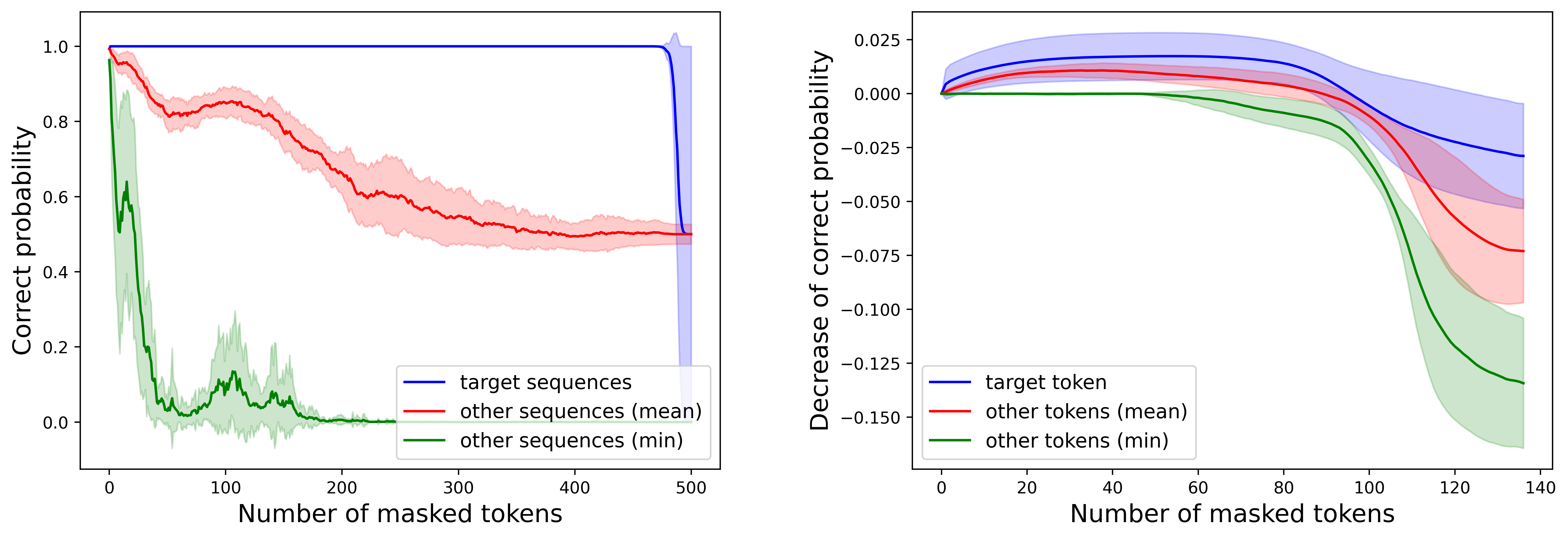
Figure 6.1: The experimental results. Left: We choose one target sequence from the test data, and repeatedly mask the tokens with less importance. Then, the probability of correct classification decreases slowly, which means the essential tokens for the classification are limited. On the other hand, if we mask tokens at the same position for other sequences, the accuracy decreases faster. This indicates that the model can select the important tokens depending on the input. Right: We fix one target token for each sequence, and repeatedly mask the input tokens with less importance. Then, the probability of correct prediction decreases slower for the chosen token than the other tokens. This reveals that the important tokens to pay attention is different depending on the output token.

To demonstrate that our theory is compatible with the real-world tasks, we conducted two numerical experiments. We utilize the pretrained model of Hyena provided by Nguyen et al. (2024), which is trained via the next token prediction task with the nucleic acid base sequences. We fine-tune the model using Genomic Benchmark dataset (Grešová et al., 2023). Additional description on the experimental setting can be found in Appendix I.

First, we verify that SSMs can select important tokens depending on the input. We fine-tune the model with the binary classification task. Then, we choose one sequence in the test data and plot the transition of the probability of correct classification when we repeatedly mask the input tokens that do not affect the classification result. Additionally, we observe how the correctness for other sequences changes when we mask the same tokens as the chosen sequence.

The result is shown on the left of Figure 6.1. We can see that SSMs can classify the sequences even if we mask most of the tokens. This indicates that the number of important tokens to classify the sequence is small. Moreover, the accuracies for other sequences decrease when there are a few tokens left, which means that the important tokens of other sequences differ from the chosen sequence.

Second, we demonstrate the ability of SSMs to extract important tokens depending on the output token. We consider the task to predict the masked token at the last of sequence. Then, we choose one token for each sequence and plot the transition of the probability of correct prediction when we repeatedly mask the tokens whose impact on the prediction is small. Additionally, we plot the transition of the correctness for other tokens when we mask the the tokens at the same positions.

We show the result in the right part of Figure 6.1. We can notice that the accuracy for the chosen token decreases slower than the other tokens. This reveals that the important tokens to pay attention to are different depending on the position of the output token, and SSMs can adaptively extract the important tokens depending on the output token.

7 Conclusion

In this paper, we theoretically explore the possibility of SSMs as an alternative to Transformers. To this end, we established the theory on the approximation and estimation ability of SSMs for a certain class. In addition to the function spaces considered in the previous work, we extend the piecewise $\gamma$-smooth function class to include the case where the importance of a token can change depending on the output token. Consequently, we prove that SSMs have the same estimation ability as Transformers for those function classes.

Limitations and future works

We investigate the ability of ERM estimators, and did not discuss whether the SSMs can be optimized efficiently. Analyzing how the optimization algorithm works for SSMs is an possible direction for future work. Additionally, we did not investigate the other types of models that is said to be an alternative to Transformers, such as SSMs with data-dependent filters (like Mamba (Gu and Dao, 2023)) and linear attention (Katharopoulos et al., 2020). Future research could focus on the comparison between those models and SSMs with gated convolution.

—— Appendix ——

Appendix A Extension to ordinary SSM filter

In this section, we describe how to extend our setting to the ordinary SSM filter. More specifically, our setting with embedding dimension $D$ can be extended to the ordinary SSM filter with embedding dimension $4D$.

For simplicity, we consider the case $D=1$. We constuct the parameters $\mathsf{A},\mathsf{B},\mathsf{C},\mathsf{D}\in\mathbb{R}^{2\times 2}$ to make the filter $h_{t}\coloneqq\mathsf{C}\mathsf{A}^{t}\mathsf{B}+\mathsf{D}\delta_{t-n}$ same as the filter defined in Section 3. Let us set $\mathsf{D}=0$, and

$$\mathsf{A}=\matrixquantity[\cos\quantity(\frac{2\pi a_{1,1}}{U})&-\sin\quantity(\frac{2\pi a_{1,1}}{U})&0&0\\ \sin\quantity(\frac{2\pi a_{1,1}}{U})&\cos\quantity(\frac{2\pi a_{1,1}}{U})&0&0\\ 0&0&\cos\quantity(\frac{2\pi a_{1,2}}{U})&-\sin\quantity(\frac{2\pi a_{1,2}}{U})\\ 0&0&\sin\quantity(\frac{2\pi a_{1,2}}{U})&\cos\quantity(\frac{2\pi a_{1,2}}{U})].$$

Then, we have

$$\mathsf{A}^{t}=\matrixquantity[\cos\quantity(\frac{2\pi a_{1,1}t}{U})&-\sin\quantity(\frac{2\pi a_{1,1}t}{U})&0&0\\ \sin\quantity(\frac{2\pi a_{1,1}t}{U})&\cos\quantity(\frac{2\pi a_{1,1}t}{U})&0&0\\ 0&0&\cos\quantity(\frac{2\pi a_{1,2}t}{U})&-\sin\quantity(\frac{2\pi a_{1,2}t}{U})\\ 0&0&\sin\quantity(\frac{2\pi a_{1,2}t}{U})&\cos\quantity(\frac{2\pi a_{1,2}t}{U})].$$

Therefore, if we set

$$\mathsf{B}=\matrixquantity[1&0&0&0\\ 0&0&0&0\\ 0&0&1&0\\ 0&0&0&0],\quad\mathsf{C}=\matrixquantity[c_{1,1}&0&0&0\\ 0&0&0&0\\ 0&0&0&0\\ c_{1,2}&0&0&0],$$

then we have

$$h_{t}=\matrixquantity[c_{1,1}\cos\quantity(\frac{2\pi a_{1,1}t}{U})&0&0&0\\ 0&0&0&0\\ 0&0&0&0\\ c_{1,2}\sin\quantity(\frac{2\pi a_{1,2}t}{U})&0&0&0].$$

Then, if we appropriately set $W^{V}$ and $W^{Q}$, this filter can realize the same output with our setting.

While we do not show the estimation ability for the filter above, we can easily extend our proof to derive the almost same estimation error bound for it.

Appendix B Key Insight on SSMs with Gated Convolution

Before starting the proof, we show the key insight on SSMs with gated convolution.

Suppose $f\colon\mathbb{R}^{d}\to\mathbb{R}^{2n},x\mapsto\quantity[\phi_{A}^{(1)}(x),\ldots,\phi_{A}^{(n)}(x),\phi_{B}^{(1)}(x),\ldots,\phi_{B}^{(n)}(x)]$ is a fully connected neural network. Additionally, let $g\in\mathcal{C}(U,D,B)$ with $D=2n$. Recall that $g$ is defined as

$$g(X)=\quantity(W^{Q}X)\odot\quantity(H\ast\quantity(W^{V}X))\quad(X\in\mathbb{R}^{2n\times\infty}),$$

where $H\in\mathbb{R}^{2n\times 2n}$ is a filter defined by

$$H_{k,j}\coloneqq c_{1,k}\cos\quantity(\frac{2\pi j\cdot a_{1,k}}{U})+c_{2,k}\sin\quantity(\frac{2\pi j\cdot a_{2,k}}{U}).$$

Let us set the parameters $W^{Q},W^{V}\in\mathbb{R}^{2n\times 2n},c_{1},c_{2}\in\mathbb{R}^{2n}$ in $g$ as

where $S\subseteq[n]$ and $\alpha_{1},\ldots,\alpha_{n}\in\mathbb{R}$. Then, for any input $X\coloneqq\quantity[x_{t}]_{t=-\infty}^{0}\in\mathbb{R}^{2n\times\infty}$, we have

$$(g\circ f(X))_{0}=\matrixquantity[\sum_{t=-U}^{0}\alpha_{1}\cdot\psi^{(1)}(t/U)\phi_{A}^{(1)}(x_{t})\phi_{B}^{(1)}(x_{0})\\ \vdots\\ \sum_{t=-U}^{0}\alpha_{n}\cdot\psi^{(n)}(t/U)\phi_{A}^{(n)}(x_{t})\phi_{B}^{(n)}(x_{0})\\ 0\\ \vdots\\ 0],$$

where

$$\psi^{(k)}(s)\coloneqq\begin{cases}\cos(2\pi a_{1,k}\cdot s)&(k\in S),\\ \sin(2\pi a_{2,k}\cdot s)&(k\notin S).\end{cases}$$

Therefore, we can see that, for any function $K\colon\mathbb{R}^{2n+1}\to\mathbb{R}$ that can be approximated by the form of

$$K(t,x,y)=\sum_{k=1}^{n}\alpha_{k}\cdot\psi^{(k)}(t/U)\phi_{A}^{(k)}(x)\phi_{B}^{(k)}(y),$$

one FNN and one SSM with gated convolution can approximate its summation over

$$(t,x,y)=\quantity(0,x_{0},x_{0}),\quantity(-1,x_{-1},x_{0}),\ldots,\quantity(-U,x_{-U},x_{0}),$$

i.e.,

$$\sum_{t=-U}^{0}K(t,x_{t},x_{0}).$$

In the following proof, we use this fact for sevaral times as described below.

Extracting a token at a specific position

We can extract one token from $x_{0},x_{-1},\ldots,x_{-U}$ by setting $K$ to satisfy

$$K(t,x,y)\approx\begin{cases}x\quad(t=t_{0}),\\ 0\quad(t\neq t_{0}),\end{cases}$$

for some $t_{0}\in[-U:0]$.

Extracting a feature of the token with high similarity

Let $\rho\colon\mathbb{R}^{n}\times\mathbb{R}^{n}\to\mathbb{R}$ be a kernel function that measures the similarity between two vectors. Suppose that $\rho$ can be approximated by a finite sum as follows:

$$\rho(x,y)\approx\sum_{k=1}^{n}\alpha_{i}\cdot\eta_{k}(x)\eta_{k}(y).$$

Let us set $K$ to satisfy

$$K(t,x,y)\approx\sum_{k=1}^{n}x_{m}\cdot\eta_{k}(x)\cdot\eta_{k}(y),$$

for some $m\in[n]$. Then we can extract the $m$-th coordinate of the token that has the highest similarity with $x_{0}$ among $x_{-U},\ldots,x_{0}$, if the similarities between other tokens and $x$ are significantly lower. Note that $x\mapsto x_{m}\cdot\eta_{k}(x)$ can be approximated by a FNN.

Appendix C Auxiliary Lemmas

In the following discusstion, to simplify the notation, we define the function class $\Psi^{\prime}(D,B)$ by

$$\Psi^{\prime}(D,B)\coloneqq\quantity{t\mapsto\quantity[c_{1,k}\cos\quantity(2\pi a_{1,k}t)+c_{2,k}\sin\quantity(2\pi a_{2,k}t)]_{k=1}^{D}\mathrel{}\middle|\mathrel{}\norm{c}_{\infty}\leq B,\norm{a}_{\infty}\leq B.}.$$

First, we prove the following lemma, which states the properties of the $\mathrm{Softmax}$ and multi-variate Swish function.

Lemma C.1 (Properties of $\mathrm{Softmax}$ and Multi-variate Swish function).

Fix $\theta\in\mathbb{R}^{d}$. Assume that there exists an index $i^{\ast}\in[d]$ and $\delta>0$ such that $\theta_{i^{\ast}}>\theta_{i}+\delta$ for all $i\neq i^{\ast}$. Then, the following two statements hold:

1. (Lemma C.1 of Takakura and Suzuki (2023)) It holds

   $$\sum_{i=1}^{d}\absolutevalue{\mathrm{Softmax}(\theta)_{i}-\delta_{i,i^{\ast}}}\leq 2d\exp(-\delta).$$

2. For any $x\in[0,1]^{d}$, it holds

   $$\absolutevalue{\sum_{i=1}^{d}\mathrm{Softmax}(\theta)_{i}\cdot x_{i}-\max\{x_{1},\ldots,x_{d}\}}\leq 2d^{2}\exp(-\delta).$$

Proof.

We prove the second one. Using the first argument, we have

$$\absolutevalue{\sum_{i=1}^{d}\mathrm{Softmax}(\theta)_{i}\cdot x_{i}-\max\{x_{1},\ldots,x_{d}\}}$$

$$\quad\leq\absolutevalue{\sum_{i\neq i^{\ast}}\mathrm{Softmax}(\theta)_{i}\cdot x_{i}+\quantity(\mathrm{Softmax}(\theta)_{i^{\ast}}\cdot x_{i^{\ast}}-\max\{x_{1},\ldots,x_{d}\})}$$

$$\quad=\absolutevalue{\sum_{i\neq i^{\ast}}\mathrm{Softmax}(\theta)_{i}\cdot x_{i}+\quantity(\mathrm{Softmax}(\theta)_{i^{\ast}}\cdot x_{i^{\ast}}-\delta_{i,i^{\ast}}x_{i^{\ast}})}$$

$$\quad\leq\sum_{i\neq i^{\ast}}\mathrm{Softmax}(\theta)_{i}\cdot x_{i}+\absolutevalue{\mathrm{Softmax}(\theta)_{i^{\ast}}-\delta_{i,i^{\ast}}}\cdot x_{i^{\ast}}$$

$$\quad\leq\sum_{i=1}^{d}\absolutevalue{\mathrm{Softmax}(\theta)_{i}-\delta_{i,i^{\ast}}}\cdot x_{i}$$

$$\quad\leq 2d^{2}\exp(-\delta),$$

which completes the proof. ∎

The following lemma shows the approximation ability of FNN for some elementary functions.

Lemma C.2 (Lemma F.6, Lemma F.7, Lemma F.12 of Oko et al. (2023), Corollary 4.2 of Perekrestenko et al. (2018)).

The following statements hold:

1. Let $d\geq 2,C\geq 1,\epsilon_{\mathrm{error}}\in(0,1]$. For any $\epsilon>0$, there exists a neural network $f_{\mathrm{mult}}\in\Psi(L,W,S,B)$ with

   $$L\lesssim(\log\epsilon^{-1}+d\log C)\cdot\log d,\quad W\lesssim d,\quad S\lesssim d\log\epsilon^{-1}+d\log C,\quad\log B\lesssim d\log C,$$

   such that, for any $x\in[0,C]^{d}$ and $x\in\mathbb{R}^{d}$ with $\norm{x-x^{\prime}}_{\infty}\leq\epsilon_{\mathrm{error}}$, it holds

   $$\absolutevalue{f_{\mathrm{mult}}(x^{\prime})-\prod_{i=1}^{d}x_{i}}\leq\epsilon+d\cdot C^{d}\cdot\epsilon_{\mathrm{error}}.$$

2. For any $\epsilon\in(0,1)$, there exists $f_{\mathrm{rec}}\in\Psi(L,W,S,B)$ with

   $$L\lesssim\log^{2}\epsilon^{-1},\quad W\lesssim\log^{3}\epsilon^{-1},\quad S\lesssim\log^{4}\epsilon^{-1},\quad\log B\lesssim\log\epsilon^{-1},$$

   such that, for any $x\in[\epsilon,\epsilon^{-1}]$ and $x^{\prime}\in\mathbb{R}$, it holds

   $$\absolutevalue{f_{\mathrm{rec}}(x^{\prime})-\frac{1}{x}}\leq\epsilon+\frac{\absolutevalue{x^{\prime}-x}}{\epsilon^{2}}.$$

3. For any $\epsilon>0$, there exists $f_{\exp}\in\Psi(L,W,S,B)$ with

   $$L\lesssim\log^{2}\epsilon^{-1},\quad W\lesssim\log\epsilon^{-1},\quad S\lesssim\log^{2}\epsilon^{-1},\quad\log B\lesssim\log^{2}\epsilon^{-1},$$

   such that, for any $x,x^{\prime}\geq 0$, it holds

   $$\absolutevalue{f_{\exp}(x^{\prime})-\exp(x)}\leq\epsilon+\absolutevalue{x^{\prime}-x}.$$

4. For any $\epsilon>0,a>0,b\in\mathbb{R},C\geq 1$, there exists $f_{\cos}\in\Psi(L,W,S,B)$ with

   $$L\lesssim\log^{2}\epsilon^{-1}+\log(aD+b),\quad W\lesssim 1,$$

   $$S\lesssim\log^{2}\epsilon^{-1}+\log(aD+b),\quad\log B\lesssim\max\quantity{1,\log\absolutevalue{b/a}},$$

   such that, for any $x\in[-D,D]$, it holds

   $$\absolutevalue{f_{\cos}(x)-\cos(ax+b)}\leq\epsilon.$$

The following is a famous fact that there exists a neural network that realize the clipping function.

Lemma C.3.

Let $a,b\in\mathbb{R}$. There exists a neural neural network $f_{\mathrm{clip}}\in\Psi(L,W,S,B)$ with

$$L\lesssim 1,\quad W\lesssim 1,\quad S\lesssim 1,\quad B\lesssim\absolutevalue{a}+\absolutevalue{b},$$

such that, for any $x\in\mathbb{R}$, it holds

$$f_{\mathrm{clip}}(x)=\begin{cases}a&\quad\text{if $x\leq a$},\\ x&\quad\text{if $a\leq x\leq b$},\\ b&\quad\text{if $b\leq x$}.\end{cases}$$

Lastly, we state the following lemma, which shows that the dirac delta function can be approximated by a neural network.

Lemma C.4.

There exists $N\in\mathbb{N}$ and FNNs $\phi_{n},\phi^{\prime}_{n},\phi^{\prime\prime}_{n}\in\Psi_{1,1}(L,W,S,B),~{}\psi_{n},\psi^{\prime}_{n}\in\Psi^{\prime}(1,B)~{}(n=1,\ldots,N)$ with

$$N\lesssim\log\epsilon^{-1},$$

$$L\lesssim\log^{2}\epsilon^{-1}\log^{2}\kappa,\quad W\lesssim\log^{2}\epsilon^{-1},\quad S\lesssim\log^{4}\epsilon^{-1}\log^{2}\kappa,\quad\log B\lesssim\log\epsilon^{-1}\log\kappa,$$

$$L^{\prime}=1,\quad W^{\prime}\lesssim\log^{2}\epsilon^{-1},\quad S^{\prime}\lesssim\log^{2}\epsilon^{-1},$$

such that,

• for any $t,x\in\mathbb{R}$, it holds

  $$\absolutevalue{\exp(-\kappa\cdot\sin^{2}\quantity(\frac{\pi}{2}(t-x)))-\sum_{n=1}^{N}\psi_{n}(t)\phi_{n}(x)}\lesssim\epsilon,$$

• for any $x,y\in\mathbb{R}$, it holds

  $$\absolutevalue{\exp(-\kappa\cdot\sin^{2}\quantity(\frac{\pi}{2}(x-y)))-\sum_{n=1}^{N}\phi^{\prime}_{n}(x)\phi^{\prime\prime}_{n}(y)}\lesssim\epsilon,$$

• for any $t\in[-1,1]$, it holds

  $$\absolutevalue{\exp(-\kappa\cdot\sin^{2}\quantity(\frac{\pi t}{2}))-\sum_{n=1}^{N}\psi^{\prime}_{n}(t)}\lesssim\epsilon.$$

Proof.

The first part of the proof is inspired by Lemma F.12 of Oko et al. (2023). Let us set $A=\log 3\epsilon^{-1}$. The Taylor expansion of $\exp$ shows that, for any $x\in[0,A]$, it holds

$$\absolutevalue{\exp(-x)-\sum_{n=0}^{N-1}\frac{(-1)^{n}}{n!}x^{n}}\leq\frac{A^{N}}{N!}.$$

Additionally, we can evaluate the right-hand side as $A^{k}/k!\leq\quantity(\mathrm{e}A/k)^{k}$. Therefore, if we set $N=\max\quantity{2\mathrm{e}A,\lceil\log_{2}3\epsilon^{-1}\rceil}$, the error can be bounded by $\epsilon/3$. Moreover, for $x>A$, we have

$$\absolutevalue{\exp(-x)-\sum_{n=0}^{N-1}\frac{(-1)^{n}}{n!}x^{n}} \leq\absolutevalue{\exp(-x)-\exp(-A)}+\absolutevalue{\exp(-A)-\sum_{n=0}^{N-1}\frac{(-1)^{n}}{n!}x^{n}}$$

$$\leq\frac{\epsilon}{3}+\frac{2\epsilon}{3}=\epsilon.$$

Next, let us approximate $\displaystyle\sum_{n=0}^{N-1}\frac{(-\kappa)^{n}}{n!}\sin^{2n}\quantity(\frac{\pi}{2}(t-x))$. We use the fact that

$$\sin^{2n}(x) =\quantity(\frac{\mathrm{e}^{ix}-\mathrm{e}^{-ix}}{2})^{2n}=\frac{1}{2^{2n}}\sum_{k=0}^{2n}\binom{2n}{k}(-1)^{k}\mathrm{e}^{i(2k-2n)x}$$

$$=\frac{(-1)^{n}}{2^{2n}}\binom{2n}{n}+\sum_{k\geq n+1}\frac{(-1)^{k}}{2^{2n-1}}\binom{2n}{k}\cos\quantity((2k-2n)x),$$

where $c_{n}=1$ if $n$ is even and $c_{n}=0$ if $n$ is odd. Thus, we have

$$\sum_{n=0}^{N-1}\frac{(-\kappa)^{n}}{n!}\sin^{2n}\quantity(\frac{\pi}{2}(t-x))$$

$$\quad=\sum_{n=0}^{N-1}\frac{\kappa^{n}}{n!2^{2n}}\binom{2n}{n}+\sum_{n=0}^{N-1}\sum_{k\geq n+1}\frac{(-\kappa)^{n}}{n!}\frac{1}{2^{2n-1}}\binom{2n}{k}\cos\quantity(\pi(k-n)(t-x))$$

$$\quad=\sum_{n=0}^{N-1}\frac{\kappa^{n}}{n!2^{2n}}\binom{2n}{n}+\sum_{n=0}^{N-1}\sum_{k\geq n+1}\frac{(-\kappa)^{n}}{n!}\frac{1}{2^{2n-1}}\binom{2n}{k}\Biggl{(}\cos\quantity(\pi(k-n)t)\cos\quantity(\pi(k-n)x)$$

$$\hskip 227.62204pt+\sin\quantity(\pi(k-n)t)\sin\quantity(\pi(k-n)x)\biggr{)},$$

which is decomposed into the sum of products of functions of $t$ and $x$. Since

$$\absolutevalue{\frac{(-\kappa)^{n}}{n!}\frac{1}{2^{2n-1}}\binom{2n}{k}}\leq\frac{\kappa^{n}}{n!2^{n}}\frac{(2n)!}{k!(2n-k)!}\leq\frac{\kappa^{n}}{n!2^{n}}\frac{2^{n}(n!)^{2}}{(\max(k,2n-k))!}=\frac{\kappa^{n}}{n!2^{n}}\frac{2^{n}(n!)^{2}}{n!}\leq\kappa^{N},$$

we can see that, there exists $C_{0},C_{n,k}~{}(n\in[N],k\in[0:n/2])$ with

$$C_{0}\leq\kappa^{N},\quad C_{n,k}\leq\kappa^{N},$$

such that

$$\sum_{n=0}^{N-1}\frac{(-\kappa)^{n}}{n!}\sin^{2n}\quantity(\frac{\pi}{2}(t-x)) =C_{0}+\sum_{n=0}^{N-1}\sum_{k\geq(n+1)/2}C_{n,k}\bigl{(}\cos\quantity(\pi(k-n)t)\cos\quantity(\pi(k-n)x)$$

$$\hskip 113.81102pt+\sin\quantity(\pi(k-n)t)\sin\quantity(\pi(k-n)x)\bigr{)}.$$

The second equation to be proved is already obtained setting $x=0$.

Finally, we approximate each term using neural networks. Lemma C.2 implies that, for any $n,k$ and $\epsilon>0$, there exists a neural network $\phi_{1,n,k},\phi_{2,n,k}\in\Psi_{1,1}(L,W,S,B)$ with

$$L\lesssim N^{2}\log^{2}\kappa+\log^{2}\epsilon^{-1},\quad W\lesssim 1,\quad S\lesssim N^{2}\log^{2}\kappa+\log^{2}\epsilon^{-1},\quad\log B\lesssim 1,$$

such that

$$\absolutevalue{\cos(\pi(k-n)x)-\phi_{1,n,k}(x)}\leq\epsilon/(N^{2}\kappa^{N}),\quad\absolutevalue{\sin(\pi(k-n)x)-\phi_{2,n,k}(x)}\leq\epsilon/(N^{2}\kappa^{N}).$$

Then, if we approximate $\exp(-\kappa\cdot\cos(2\pi(t-x)))$ by

$$C_{0}+\sum_{n=0}^{N-1}\sum_{k\geq(n+1)/2}C_{n,k}\quantity(\cos\quantity(\pi(k-n)t)\phi_{1,n,k}(x)+\sin\quantity(\pi(k-n)t)\phi_{2,n,k}(x)),$$

the error can be bounded by

$$\epsilon+\sum_{n=0}^{N-1}\sum_{k\geq(n+1)/2}C_{n,k}\cdot\frac{2\epsilon}{N^{2}\kappa^{N}}\leq\epsilon+N^{2}\kappa^{N}\cdot\frac{2\epsilon}{N^{2}\kappa^{N}}\leq 3\epsilon,$$

which completes the proof. ∎

Appendix D Proof of Theorem 4.2

Given a smoothness function $\gamma\colon\mathbb{N}_{0}^{d\times\infty}\to\mathbb{R}$, we define

$$I(T,\gamma) \coloneqq\{(i,j)\mid\exists s\in\mathbb{N}_{0}^{d\times\infty}\text{ such that }s_{ij}\neq 0,\gamma(s)<T\},$$

$$d_{\max} \coloneqq|I(T,\gamma)|.$$

The feature extraction map $\Gamma\colon\mathbb{R}^{d\times\infty}\to\mathbb{R}^{d_{\max}}$ is defined as

$$\Gamma(X)=[X_{i_{1},j_{1}},\ldots,X_{i_{d_{\max}},j_{d_{\max}}}].$$

The following lemma shows that, if FNN receives finite number of "important" features, it can approximate $\gamma$-smooth functions and piecewise $\gamma$-smooth functions. This is mainly due to the condition $\|a\|_{wl^{\alpha}}\leq 1$, which induces sparsity of important features.

Lemma D.1 (Theorem D.3 in Takakura and Suzuki (2023)).

Suppose that the target functions $f\in\mathcal{F}_{p,\theta}^{\gamma}$ and $g\in\mathcal{P}_{p,\theta}^{\gamma}$ satisfy $\norm{f}_{\infty}\leq R$ and $\norm{g}_{\infty}\leq R$, where $R>0$ and $\gamma$ is the mixed or anisotropic smoothness and the smoothness parameter $a$ satisfies $\norm{a}_{wl^{\alpha}}\leq 1$. For any $T>0$, there exist FNNs $\hat{f}_{T},\hat{g}_{T}\in\Psi(L,W,S,B)$ such that

$$\norm{\hat{f}_{T}\circ\Gamma-f}_{2,P_{X}} \lesssim 2^{-T},$$

$$\norm{\hat{g}_{T}\circ\Gamma\circ\Pi-g}_{2,P_{X}} \lesssim 2^{-T},$$

where

$$L \sim\max\quantity{T^{2/\alpha},T^{2}},W\sim T^{1/\alpha}2^{T/a^{\dagger}},$$

$$S \sim T^{2/\alpha}\max\quantity{T^{2/\alpha},T^{2}}2^{T/a^{\dagger}},\log B\sim T^{1/\alpha}.$$

From this lemma, we can see that, if the the convolution layer can approximate $\Gamma$, the SSM can give important features to the FNN, and the FNN can approximate the target function.

Now, we prove Theorem 4.2.

Proof of Theorem 4.2.

Firstly, we construct the embedding layer $\mathrm{Emb}\colon\mathbb{R}^{d\times\infty}\to\mathbb{R}^{D\times\infty}$. Set the embedding dimension $D$ as $\max\{d,d_{\max}\}+1$. We set $E_{1}\in\mathbb{R}^{D\times d}$ to satisfy

$$E_{1}x=[x_{1},~{}\ldots,~{}x_{d},~{}0,\underbrace{0,~{}\ldots,~{}0}_{D-d-1\text{ elements}}]^{\top}.$$

for $x=[x_{1},\ldots,x_{d}]\in\mathbb{R}^{d}$. Additionally, we set $E_{2}\in\mathbb{R}^{D}$ to satisfy

$$E_{2}=[\underbrace{0,~{}\ldots,~{}0}_{d\text{ elements}},~{}1,\underbrace{0,~{}\ldots,~{}0}_{D-d-1\text{ elements}}]^{\top}.$$

Note that $\norm{E_{1}}_{\infty}=\norm{E_{2}}_{\infty}=1$. Then, the constructed embedding layer $\mathrm{Emb}$ is represented as follows:

$$\mathrm{Emb}(X)=\begin{bmatrix}\cdots&x_{t}&\cdots\\ \cdots&1&\cdots\\ \cdots&0&\cdots\\ \vdots&\vdots&\vdots\\ \cdots&0&\cdots\\ \end{bmatrix}\in\mathbb{R}^{D\times\infty}.$$

Secondly, we construct the gated convolution layer. The role of this layer is to approximate the feature extractor $\Gamma$. The weight matrix $W^{V}\in\mathbb{R}^{D\times|X|}$ is set to extract the important “dimensions” ($i_{1},\ldots,i_{d_{\max}}$). More precisely, we set $W_{V}$ to satisfy

$$W^{V}y=[y_{i_{1}},\ldots,y_{i_{d_{\max}}},\underbrace{0,~{}\ldots,~{}0}_{D-d_{\max}\text{ elements}}]\in\mathbb{R}^{D}$$

for $y=[y_{1},\ldots,y_{D}]\in\mathbb{R}^{D}$. Then, the resulted projection is represented as follows:

$$W^{V}(\mathrm{Emb}(X))=\begin{bmatrix}\cdots&X_{t,i_{1}}&\cdots\\ \vdots&\vdots&\vdots\\ \cdots&X_{t,i_{d_{\max}}}&\cdots\\ \cdots&0&\cdots\\ \vdots&\vdots&\cdots\\ \cdots&0&\cdots\\ \end{bmatrix}\in\mathbb{R}^{D\times\infty}.$$

Next, we construct the convolution filter. From the assumption $a_{ij}=\Omega(\log(|j|+1))$, we can choose the window size $U\in\mathbb{N}$ such that

$$\log U\sim T\mbox{\quad and\quad}a_{ij}\leq T\Longrightarrow j\leq U.$$

Lemma C.4 shows that, for each $j_{m}~{}(m=1,\ldots,d_{\max})$, for any $\epsilon>0,\kappa>0$, there exists $k_{m}\in\Psi^{\prime}(W^{\prime},B)$ with

$$W^{\prime}\lesssim\log^{2}\epsilon^{-1},\quad B\lesssim\log\epsilon^{-1}\log\kappa$$

such that

$$\max_{j=0,\ldots,U}\absolutevalue{k_{m}\quantity(\frac{j}{U})-\exp(-\kappa\cdot\sin^{2}\quantity(\frac{\pi}{2}\quantity(\frac{j}{U}-\frac{j_{m}}{U})))}\lesssim\epsilon.$$

Now, if $\absolutevalue{j-j_{m}}\geq 1$, it holds

$$\exp(-\kappa\cdot\sin^{2}\quantity(\frac{\pi}{2}\quantity(\frac{j}{U}-\frac{j_{m}}{U})))\leq\exp(-\kappa\cdot\quantity(\frac{2}{\pi}\cdot\frac{\pi}{2}\cdot\frac{1}{U})^{2})=\exp(-\frac{\kappa}{U^{2}}),$$

and, if $j=j_{m}$, it holds

$$\exp(-\kappa\cdot\sin^{2}\quantity(\frac{\pi}{2}\quantity(\frac{j}{U}-\frac{j_{m}}{U})))=1.$$

Therefore, if we set $\kappa=U^{2}\log\epsilon^{-1}$, we have

$$\max_{j=0,\ldots,U}\absolutevalue{k_{m}\quantity(\frac{j}{U})-\delta_{j_{m}}(j)}\lesssim 2\epsilon,$$

where $\delta_{j^{\prime}}$ is the function defined by

$$\delta_{j^{\prime}}(j)=\begin{cases}1&\text{if }j=j^{\prime},\\ 0&\text{otherwise}.\end{cases}$$

This inequality show that the filter $k$ can approximately extract the important tokens.

Finally, we set the weight matrix $W^{Q}$ by

$$W^{Q}_{i,j}=\begin{cases}1&\text{if $j=d+1$}\\ 0&\text{otherwise},\end{cases}$$

which results in $W^{Q}(\mathrm{Emb}(X))=[1,\ldots,1]^{\top}$ and

$$g_{1}\circ\mathrm{Emb}(X) =W^{Q}(\mathrm{Emb}(X))\odot(\beta^{(1)}\ast W^{(0)}(\mathrm{Emb}(X)))$$

$$=\beta^{(1)}\ast W^{(0)}(\mathrm{Emb}(X))$$

$$=[z_{t}]_{t=-\infty}^{\infty}\in\mathbb{R}^{D\times\infty},$$

$$z_{t} =\sum_{s=0}^{U-1}k(s)\sum_{i=1}^{D}W^{(0)}_{i,t-s}X_{i,t-s}$$

$$=\begin{bmatrix}\sum_{s=0}^{U-1}(k(s))_{1}X_{i_{1},t-s}\\ \vdots\\ \sum_{s=0}^{U-1}(k(s))_{d_{\max}}X_{i_{d_{\max}},t-s}\\ 0\\ \vdots\\ 0\end{bmatrix}.$$

Thirdly, we construct the FNN layer. From Lemma D.1, there exists an FNN $\hat{f}\in\Psi(L,W,S,B)$ such that

$$\norm{\hat{f}\circ\Gamma-F_{0}^{\circ}}_{2,P_{X}}\lesssim 2^{-T},$$ (D.1)

where

$$\begin{aligned} L&\sim\max\quantity{T^{2/\alpha},T^{2}},W\sim T^{1/\alpha}2^{T/a^{\dagger}},\\ S&\sim T^{2/\alpha}\max\quantity{T^{2/\alpha},T^{2}}2^{T/a^{\dagger}},\log B\sim T^{1/\alpha}.\end{aligned}$$ (D.2)

Let $C\colon\mathbb{R}^{D}\to\mathbb{R}^{d}$ be a linear map such that

$$Cy=[y_{1},\ldots,y_{d_{\max}}]^{\top}$$

for $y=[y_{1},\ldots,y_{D}]^{\top}\in\mathbb{R}^{D}$, and we set $f_{1}\coloneqq\hat{f}\circ C$. Note that $f_{1}\in\Psi(L,W,S,B)$ for $L,W,S,B$ defined in (D.2). The constructed data-controlled SSM $\hat{F}_{t}~{}(t\in\mathbb{Z})$ is represented as follows:

$$\hat{F}_{t}(X)=f_{1}(z_{t})=\hat{f}\circ C(z_{t})=\hat{f}\circ\hat{\Gamma}\circ\Sigma_{t}(X),$$

where

$$\hat{\Gamma}(X)=\left[\sum_{s=0}^{U-1}(k(s))_{m}X_{i_{m},-s}\right]_{m=1}^{d_{\max}}\in\mathbb{R}^{d_{\max}}.$$

Now, we evaluate the error between the target function $F^{\circ}_{t}$ and the constructed model $\hat{F}_{t}$ for $t\in\mathbb{Z}$. Due to the shift-equivariance of $F^{\circ}$, we have $F_{t}^{\circ}=F_{0}^{\circ}\circ\Sigma_{t}$. Additionally, we can easily check that $\hat{F}_{t}$ is also shift-equivariant, i.e., $\hat{F}_{t}(X)=\hat{F}_{0}(X\circ\Sigma_{t})$. Moreover, since $P_{X}$ is also shift-equivariant, we have $\norm{u}_{2,P_{X}}=\norm{u\circ\Sigma_{t}}_{2,P_{X}}$ for any $t\in\mathbb{Z}$ and $u\colon\mathbb{R}^{d\times\infty}\to\mathbb{R}^{d}$ such that $\norm{u}_{2,P_{X}}<\infty$. Therefore, it holds

$$\norm{\hat{F}_{t}-F_{t}^{\circ}}_{2,P_{X}}=\norm{\hat{F}_{0}\circ\Sigma_{t}-F_{0}^{\circ}\circ\Sigma_{t}}$$

=∥^F0-F0∘∥2,PX

for any $t\in\mathbb{Z}$. Therefore, it is sufficient to evaluate $\norm{\hat{F}_{0}-F_{0}^{\circ}}_{2,P_{X}}$. We evaluate the error by separating into two terms:

$$\norm{\hat{F}_{0}-F_{0}^{\circ}}_{2,P_{X}}\leq\norm{\hat{F}_{0}-\hat{f}\circ\Gamma}_{2,P_{X}}+\norm{\hat{f}\circ\Gamma-F_{0}^{\circ}}_{2,P_{X}}.$$

The second term can be bounded by (D.1), so we evaluate the first term. Since $\hat{f}\in\Psi(L,W,S,B)$ is $(BW)^{L}$-lipschitz continuous, for any $X\in[0,1]^{d\times\infty}$, we have

$$\left|\hat{F}_{0}(X)-\hat{f}\circ\Gamma(X)\right|=\left|\hat{f}(\hat{\Gamma}(X))-\hat{f}(\Gamma(X))\right|\leq(BW)^{L}\norm{\hat{\Gamma}(X)-\Gamma(X)}_{\infty}.$$

Since $X\in[0,1]^{d\times\infty}$, it holds

$$\norm{\hat{\Gamma}(X)-\Gamma(X)}_{\infty} =\max_{m=1,\ldots,d_{\max}}\left|\sum_{s=0}^{U-1}(k(s))_{m}X_{i_{m},-s}-\delta_{j_{m}}(s)X_{i_{m},-s}\right|$$

$$\leq\max_{m=1,\ldots,d_{\max}}\sum_{s=0}^{U-1}\left|(k(s))_{m}-\delta_{j_{m}}(s)\right|$$

$$\leq U\epsilon.$$

By setting $\epsilon=2^{-T}/U$, we have

$$\left|\hat{F}_{0}(X)-\hat{f}\circ\Gamma(X)\right|\leq\norm{\hat{\Gamma}(X)-\Gamma(X)}_{\infty}\leq 2^{-T}$$

for any $X\in[0,1]^{d\times\infty}$. Therefore, it holds

$$\norm{\hat{F}_{0}-F_{0}^{\circ}}_{2,P_{X}} \leq\norm{\hat{F}_{0}-\hat{f}\circ\Gamma}_{2,P_{X}}+\norm{\hat{f}\circ\Gamma-F_{0}^{\circ}}_{2,P_{X}}$$

$$\leq\sup_{X\in[0,1]^{d\times\infty}}\left|\hat{F}_{0}(X)-\hat{f}\circ\Gamma(X)\right|+\norm{\hat{f}\circ\Gamma-F_{0}^{\circ}}_{2,P_{X}}$$

$$\lesssim 2^{-T}.$$

Finally, we evaluate the parameters $L,W,S,B$ which controls the class of $k\in\Psi^{\prime}(W^{\prime},B)$. Since $\|a\|_{wl^{\alpha}}=\sup_{j}j^{\alpha}\bar{a}_{j}^{-1}\leq 1$, it holds

$${d_{\max}}\coloneqq\absolutevalue{\quantity{(i,j)\mathrel{}\middle|\mathrel{}\exists s\in\mathbb{N}_{0}^{d\times\infty},s_{ij}\neq 0,\gamma(s)<T}}\leq T^{1/\alpha}.$$

Therefore, we have

$$W^{\prime} ={d_{\max}}\cdot\log^{2}\epsilon^{-1}\lesssim T^{2+1/\alpha},$$

$$\log B \sim\log\epsilon^{-1}\log(U^{2}\log\epsilon^{-1})\lesssim T^{2}.$$

This completes the proof. ∎

Appendix E Proof of Theorem 4.4

E.1 Proof for the case of (i) $\gamma$-smooth importance function

Proof of Theorem 4.4 for the case of (i) $\gamma$-smooth importance function.

For $T>0$, we define

$$I_{j}(T,\gamma) \coloneqq\quantity{i\mid(i,j)\in I(T,\gamma)}=\quantity{i_{1}^{(j)},\ldots,i_{\absolutevalue{I_{j}}}^{(j)}},$$

$$r_{\max}(T,\gamma) \coloneqq\max\quantity{j\in[J]\mid I_{j}(T,\gamma)\neq\emptyset},$$

Note that $r_{\max}(T,\gamma)\sim T^{1/\alpha}$ since $a_{ij}=\Omega(j^{\alpha})$.

Theorem 4.2 implies that there exist an embedding layer $\mathrm{Emb}$, an FNN $f_{1}\in\Psi(L,W,S,B)$ and a gated convolution layer $g_{1}\in\mathcal{C}(U,D,L^{\prime},W^{\prime},S,B)$ with

$$M=1,\log U\sim T,D\sim T^{1/\alpha},$$

$$L\sim T,W_{1}\sim T^{1/\alpha},$$

$$L^{\prime}\sim\max\quantity{T^{2/\alpha},T^{2}},W^{\prime}\sim T^{1/\alpha}2^{T/a^{\dagger}},$$

$$S\sim T^{2/\alpha}\max\quantity{T^{2/\alpha},T^{2}}2^{T/a^{\dagger}},\log B\sim T^{1/\alpha},$$

such that

$$f_{1}\circ g_{1}\circ\mathrm{Emb}(X)_{i}=[x_{i}^{\top},\widehat{\mu}_{i}(X),\underbrace{0,\ldots,0}_{\text{$d_{\max}$ elements}},\underbrace{-1,\ldots,-1}_{\text{$r_{\max}$ elements}}]^{\top},$$

for all $i\in\mathbb{Z}$, where $\widehat{\mu}_{i}(X)$ satisfies

$$\absolutevalue{\widehat{\mu}_{i}(X)_{-t}-(\mu_{i}(X)-1)}\lesssim 2^{-T}.$$

Intuitively, the $i$-th elements for $i=3,\ldots,2+d_{\max}$ are used to store the feature $X_{t-i,j}$ for $j\in[d]$, and the $i$-th elements for $i=3+d_{\max},\ldots,2+d_{\max}+r_{\max}$ are buffers to store which elements are already selected. Note that, for any $i\leq r_{\max}$, it holds

$$\widehat{\mu}(X)_{\pi_{\lambda}(i)}-\widehat{\mu}(X)_{\pi_{\lambda}(i+1)}\gtrsim(\mu(X)_{\pi_{\lambda}(i)}-2^{-T})-(\mu(X)_{\pi_{\lambda}(i+1)}+2^{-T})\gtrsim T^{-\beta/\alpha},$$

and $\widehat{\mu}(X)_{t}\in[-1,0]$ for all $t\in[0:V]$.

In the following, we set $U=V$. Let us set $\chi_{T}\sim\displaystyle\frac{T\log 2+2\log U}{T^{-\beta/\alpha}}$. Using Lemma C.2, we see that, there exists a neural network $\phi_{\exp}\in\Psi(L,W,S,B)$ with

$$L\lesssim T^{2(1+\beta/\alpha)}\log^{2}U,\quad W\lesssim T^{1+\beta/\alpha}\log U,\quad S\lesssim T^{2(1+\beta/\alpha)}\log^{2}U,\quad\log B\lesssim T^{2(1+\beta/\alpha)}\log^{2}U,$$

such that, for any $x\leq 0$, it holds

$$\absolutevalue{\phi_{\exp}(\chi_{T}x)-\exp(\chi_{T}x)}\leq 2^{-2T^{1+\beta/\alpha}}/U^{3}.$$

Moreover, using Lemma C.2 again, we see that there exists a neural network $\phi_{\times}$ with

$$L\lesssim T^{2(1+\beta/\alpha)}\log^{2}U,\quad W\lesssim 1,\quad S\lesssim T^{2(1+\beta/\alpha)}\log^{2}U,\quad\log B\lesssim T^{1+\beta/\alpha}\log U,$$

such that, for any $0\leq x\lesssim U^{2}\exp(T^{1+\beta/\alpha}),~{}0\leq y\lesssim 1$, it holds

$$\absolutevalue{\phi_{\times}(x,y)-xy}\leq 2^{-2T^{1+\beta/\alpha}}/U^{3}.$$

Then, for any $x\leq 0$ and $y\in[0,1]$, it holds

$$\absolutevalue{\phi_{\times}(\phi_{\exp}(\chi_{T}x),y)-\exp(\chi_{T}x)y} \leq\absolutevalue{\phi_{\times}(\phi_{\exp}(\chi_{T}x),y)-\phi_{\exp}(\chi_{T}x)y}+\absolutevalue{\phi_{\exp}(\chi_{T}x)y-\exp(\chi_{T}x)y}$$

$$\leq 2^{-2T^{1+\beta/\alpha}}/U^{3}+2^{-2T^{1+\beta/\alpha}}/U^{3}$$

$$\lesssim 2^{-2T^{1+\beta/\alpha}}/U^{3}.$$

Then, let us define $f^{\prime}_{1}$ be an FNN layer such that it holds

$$f^{\prime}_{1}\circ f_{1}\circ g_{1}(X)\circ\mathrm{Emb}(X)_{i}=[\phi_{\times}(\phi_{\exp}(\widehat{\mu}_{i}(X)),x_{i}),\underbrace{0,\ldots,0}_{\text{$d_{\max}$ elements}},\underbrace{-1,\ldots,-1}_{\text{$r_{\max}$ elements}}]^{\top}.$$

Additionally, we define

$$Z_{m}\coloneqq(f^{\prime}_{m}\circ g_{m}\circ f_{m})\circ\cdots\circ(f^{\prime}_{1}\circ g_{1}\circ f_{1})\circ\mathrm{Emb}(X),$$

for $m\in[1:r_{\max}]$. We construct remaining layers $f_{2},g_{2},f^{\prime}_{2},\ldots,f_{r_{\max}+1},g_{r_{\max}+1},f^{\prime}_{r_{\max}+1}$ to make them satisfying

$$Z_{m}=[\phi_{\times}(\phi_{\exp}(\widehat{\mu}_{i}(X)),x_{i}),\widehat{X}_{i_{1}^{(1)},j_{1}},\ldots,\widehat{X}_{i_{\absolutevalue{I_{1}}}^{(1)},j_{1}},\ldots,\widehat{X}_{i_{1}^{(m)},j_{m}},\ldots,\widehat{X}_{i_{\absolutevalue{I_{m}}}^{(m)},j_{m}},\underbrace{0,\ldots,0}_{d_{\max}-\sum_{j=1}^{m}\absolutevalue{I_{j}}\text{ elements}},$$

$$\hskip 256.0748pt\widehat{j}_{1}/U,\ldots,\widehat{j}_{m}/U,\underbrace{-1,\ldots,-1}_{r_{\max}-m\text{ elements}}]^{\top},$$

where $\widehat{X}_{i_{k}^{(j_{m})},j_{m}},\widehat{j}_{m}$ are the approximation of $\widehat{X}_{i_{k}^{(j_{m})},j_{m}},\widehat{j}_{m}~{}(m=1,\ldots,M;k=1,\ldots,\absolutevalue{I_{j_{m}}})$ respectively such that

$$\absolutevalue{\widehat{X}_{i_{k}^{(j_{m})},j_{m}}-X_{i_{k}^{(j_{m})},j_{m}}}\lesssim 2^{-T},\quad\absolutevalue{\widehat{j}_{m}/U-j_{m}/U}\lesssim 2^{-3T^{1+\beta/\alpha}}/V^{5}.$$

Then, we see that

$$Z_{M}=[x_{i}^{\top},\widehat{\mu}_{i}(X),\widehat{X}_{i_{1}^{(1)},j_{1}},\ldots,\widehat{X}_{i_{\absolutevalue{I_{1}}}^{(1)},j_{1}},\ldots,\widehat{X}_{i_{1}^{(r_{\max})},j_{r_{\max}}},\ldots,\widehat{X}_{i_{\absolutevalue{I_{r_{\max}}}}^{(r_{\max})},j_{r_{\max}}},\widehat{j}_{1}/U,\ldots,\widehat{j}_{M}/U]^{\top}.$$

Hence, Lemma D.1 shows that there exists a FNN $f^{\prime}_{M}\in\Psi(L,W,S,B)$ with

$$L\lesssim\max\quantity{T^{2/\alpha},T^{2}},\quad W\lesssim T^{1/\alpha}2^{T/\alpha^{\dagger}},$$

$$S\lesssim T^{2/\alpha}\max\quantity{T^{2/\alpha,T^{2}}}2^{T/\alpha^{\dagger}},\quad\log B\lesssim T^{1/\alpha},$$

such that

$$\norm{f^{\prime}_{M}(Z_{M})-f}_{2}\lesssim 2^{-T}.$$

The same discussion as Theorem 4.2 gives the desired result.

In the following, we construct an FNN $f_{m}$ and a gated convolution layer $g_{m}$ for $m\in[1:r_{\max}]$. The proof mainly divided into two parts: (i) obtaining $\widehat{X}_{i^{(m)}_{k},j_{m}}$, i.e., the approximation of important features $X_{i^{(m)}_{k},j_{m}}~{}(k=1,\ldots,\absolutevalue{I_{m}})$ and (ii) getting $\widehat{j}_{m}$, i.e., recording which token $j_{m}$ was selected.

Picking up the important features $X_{i^{(m)}_{k},j_{m}}~{}(k=1,\ldots,\absolutevalue{I_{m}})$

Due to Lemma C.1 and the fact that $j_{m}\in[0:V]$ is an index such that $\mu_{t-j}$ ($\widehat{\mu}_{t-j}$) is the largest in $\mu_{t-j}$ ($\widehat{\mu}_{t-j})~{}(j\neq j_{1},\ldots,j_{m-1})$, for any $t\in[0:U]$ with $t\neq t_{0}$, it holds

$$\absolutevalue{\frac{\sum_{j=0}^{V}X_{i,j}\exp(\chi_{T}\cdot\widehat{\mu}_{t-j})\cdot(1-\mathbb{I}_{S}(j))}{\sum_{j=0}^{V}\exp(\chi_{T}\cdot\widehat{\mu}_{t-j})\cdot(1-\mathbb{I}_{S}(j))}-X_{i,j_{m}}}\leq 2U^{2}\exp(-\chi_{T}\cdot T^{-\beta/\alpha})\lesssim 2^{-T},$$

where $S=\quantity{j_{1},\ldots,j_{m-1}}$. Now, let us approximate

$$\frac{\sum_{j=0}^{V}X_{i,j}\exp(\chi_{T}\cdot\widehat{\mu}_{t_{i}})\cdot(1-\mathbb{I}_{S}(j))}{\sum_{j=0}^{V}\exp(\chi_{T}\cdot\widehat{\mu}_{t-i})\cdot(1-\mathbb{I}_{S}(j))}=\frac{\frac{1}{V}\sum_{j=0}^{V}X_{i,j}\exp(\chi_{T}\cdot\widehat{\mu}_{t_{i}})\cdot(1-\mathbb{I}_{S}(j))}{\frac{1}{V}\sum_{j=0}^{V}\exp(\chi_{T}\cdot\widehat{\mu}_{t-i})\cdot(1-\mathbb{I}_{S}(j))}$$

using neural networks. Using Lemma C.2, we see that, for any $\epsilon_{1}>0$, there exists a neural network $\phi_{\mathrm{rec}}\in\Psi(L,W,S,B)$ with

$$L\lesssim\log^{2}\epsilon_{1}^{-1},\quad W\lesssim\log^{3}\epsilon_{1}^{-1},\quad S\lesssim\log^{4}\epsilon_{1}^{-1},\quad\log B\lesssim\log\epsilon_{1}^{-1},$$

such that, for any $x\in[\epsilon_{1},\epsilon_{1}^{-1}]$, it holds

$$\absolutevalue{\phi_{\mathrm{rec}}(x)-\frac{1}{x}}\leq\epsilon_{1},$$

and $\phi_{\mathrm{rec}}(x)\in(0,1]$. Moreover, using Lemma C.2 again, we see that, for any $\epsilon_{3}>0$, there exists a neural network $\phi_{\mathrm{mult}}\in\Psi(L,W,S,B)$ with

$$L\lesssim\log\epsilon_{2}^{-1},\quad W\lesssim 1,\quad S\lesssim\log\epsilon_{2}^{-1},\quad\log B\lesssim 1,$$

such that, for any $x\in[0,1]^{2}$, it holds

$$\absolutevalue{\phi_{\mathrm{mult}}(x)-x_{1}x_{2}}\leq\epsilon_{2}.$$

Setting $\epsilon_{1}=\min\{\exp(-\chi_{T}),2^{-T}\},\epsilon_{2}=2^{-T}$ and

$$\phi_{\ast}\colon[\exp(-\chi_{T}),1]\times[0,1]\to\mathbb{R},(x,y)\mapsto\phi_{\mathrm{mult}}(\phi_{\mathrm{rec}}(x),y),$$

we see that $\phi_{\ast}\in\Psi(L,W,S,B)$ with

$$L\lesssim T^{2(1+\beta/\alpha)}\log^{2}U,\quad W\lesssim T^{3(1+\beta/\alpha)}\log^{3}U,\quad S\lesssim T^{4(1+\beta/\alpha)}\log^{4}U,\quad\log B\lesssim T^{1+\beta/\alpha}\log U,$$

and, for any $x\in[\exp(-\chi_{T}),\exp(\chi_{T})],y\in[0,U]$, it holds

$$\absolutevalue{\phi_{\ast}(x,y)-\frac{y}{x}} =\absolutevalue{\phi_{\mathrm{mult}}(\phi_{\mathrm{rec}}(x),y)-\frac{y}{x}}$$

$$\leq\absolutevalue{\phi_{\mathrm{mult}}(\phi_{\mathrm{rec}}(x),y)-y\phi_{\mathrm{rec}}(x)}+\absolutevalue{y\phi_{\mathrm{rec}}(x)-\frac{y}{x}}$$

$$\leq\epsilon_{2}+\epsilon_{1}\lesssim 2^{-T}.$$

Now, if we set $w(x,y)\coloneqq y/x$ for $x,y>0$, we have

$$\norm{\nabla w(x,y)}_{2}=\sqrt{\quantity(\frac{1}{x})^{2}+\quantity(-\frac{y}{x^{2}})^{2}}=\frac{1}{x}\sqrt{1+\quantity(\frac{y}{x})^{2}}.$$

Therefore, if $x\geq 1$ and $0\leq y\leq x$, it holds

$$\norm{\nabla w(x,y)}_{2}\leq\frac{1}{x}\sqrt{1+\quantity(\frac{x}{x})^{2}}=\sqrt{2}\exp(\chi_{T})\lesssim U^{2}2^{T^{1+\beta/\alpha}},$$

which means, for any $x,x^{\prime},y,y^{\prime}>0$ with $x,x^{\prime}\in[\exp(-\chi_{T}),1]$ and $0\leq y\leq x,0\leq y^{\prime}\leq x^{\prime}$, it holds

$$\absolutevalue{\frac{y}{x}-\frac{y^{\prime}}{x^{\prime}}}\lesssim U^{2}2^{T^{1+\beta/\alpha}}\quantity(\absolutevalue{x-x^{\prime}}+\absolutevalue{y-y^{\prime}}),$$

which means

$$\absolutevalue{\phi_{\ast}(x^{\prime},y^{\prime})-\frac{y}{x}} \leq\absolutevalue{\phi_{1}(x^{\prime},y^{\prime})-\frac{y^{\prime}}{x^{\prime}}}+\absolutevalue{\frac{y^{\prime}}{x^{\prime}}-\frac{y}{x}}$$

$$\lesssim 2^{-T}+U^{2}2^{T^{1+\beta/\alpha}}\quantity(\absolutevalue{x-x^{\prime}}+\absolutevalue{y-y^{\prime}})$$

Next, Lemma C.4 implies that there exists a neural networks $\phi^{\prime}_{n}\in\Psi^{\prime}(1,B)$ and $\phi_{n}\in\Psi(L,W,S,B)~{}(n=1,\ldots,N)$ with

$$N \lesssim T^{1+\beta/\alpha}\log T\log V,$$

$$L \lesssim T^{2(1+\beta/\alpha)}\log T\log^{2}V,\quad W\lesssim 1,$$

$$S \lesssim T^{2(1+\beta/\alpha)}\log T\log^{2}V,\quad\log B\lesssim 1,$$

such that, for any $t,x,\widehat{x}\in[0,1]$, it holds

$$\absolutevalue{\sum_{n=0}^{N}\phi^{\prime}_{n}(t)\phi_{n}(\widehat{x})-\exp(-\frac{V^{2}(\frac{1}{\alpha}\log T+2T^{1+\beta/\alpha}+2\log V)\cdot\sin^{2}\quantity(\frac{\pi}{2}(t-x))}{2})}$$

$$\hskip 113.81102pt\lesssim T^{-1/\alpha}2^{-2T^{1+\beta/\alpha}}/V^{2}+T^{1+\beta/\alpha}V^{3}\absolutevalue{x-\hat{x}}.$$

Since

$$\exp(-\frac{V^{2}(\frac{1}{\alpha}\log T+2T^{1+\beta/\alpha}+2\log V)\sin^{2}\quantity(\frac{\pi}{2}(t-x))}{2})$$

$$\hskip 199.16928pt\begin{cases}\leq T^{-1/\alpha}2^{-2T^{1+\beta/\alpha}}/V^{2}&\quad(\absolutevalue{t-x}\geq 1/V),\\ =1&\quad(t=x),\end{cases}$$

we have

$$\absolutevalue{\exp(-\frac{V^{2}(\frac{1}{\alpha}\log T+2T^{1+\beta/\alpha}+2\log V)\sin^{2}\quantity(\frac{\pi}{2}(t-x))}{2})-\mathbb{I}_{\quantity{x}}(t)}\lesssim 2T^{-1/\alpha}2^{-2T^{1+\beta/\alpha}}/V^{2}.$$

Therefore, we have

$$\absolutevalue{\sum_{n=1}^{N}\phi^{\prime}_{n}(t)\phi_{n}(\widehat{x})-\mathbb{I}_{\quantity{x}}(t)}\lesssim T^{-1/\alpha}2^{-(1+\beta/\alpha)T}/V^{2}+T^{1+\beta/\alpha}V^{3}\absolutevalue{x-\hat{x}}.$$

Summing up over $x=j_{1}/U,\ldots,j_{m-1}/U$, we have

$$\absolutevalue{\sum_{m^{\prime}=1}^{m-1}\sum_{i=1}^{I}\phi_{0}^{(j_{m^{\prime}},i)}(t)\phi_{1}^{(j_{m^{\prime}},i)}(\hat{j}_{m^{\prime}}/U)-\mathbb{I}_{S}(t)}$$

$$\qquad\lesssim r_{\max}\quantity(T^{-1/\alpha}2^{-2T^{1+\beta/\alpha}}/V^{2}+T^{1+\beta/\alpha}V^{3}\absolutevalue{\hat{j}_{m^{\prime}}/U-j_{m^{\prime}}/U})$$

$$\qquad\lesssim 2^{-2T^{1+\beta/\alpha}}/V^{2}.$$

Combining the results above, we have

$$\Biggl{|}\frac{1}{V}\sum_{j=0}^{V}\phi_{\times}(\phi_{\exp}(X_{i,j},\chi_{T}\widehat{\cdot}\mu_{t-j}))\cdot\quantity(1-\sum_{m^{\prime}=1}^{m-1}\sum_{i=1}^{I}\phi_{0}^{(j_{m^{\prime}},i)}(t)\phi_{1}^{(j_{m^{\prime}},i)}(\hat{j}_{m^{\prime}}/U))$$

$$\hskip 213.39566pt-\frac{1}{V}\sum_{j=0}^{V}X_{i,j}\exp(\chi_{T}\cdot\widehat{\mu}_{t-j})\cdot(1-\mathbb{I}_{S}(j))\Biggr{|}$$

$$\quad\lesssim\frac{1}{V}\sum_{j=0}^{V}\Biggl{(}\absolutevalue{\phi_{\times}(\phi_{\exp}(X_{i,j},\chi_{T}\cdot\widehat{\mu}_{t-j}))\cdot\quantity(\sum_{m^{\prime}=1}^{m-1}\sum_{i=1}^{I}\phi_{0}^{(j_{m^{\prime}},i)}(t)\phi_{1}^{(j_{m^{\prime}},i)}(\hat{j}_{m^{\prime}}/U)-\mathbb{I}_{S}(j))}$$

$$\hskip 142.26378pt+\absolutevalue{\quantity(\phi_{\times}(\phi_{\exp}(X_{i,j},\chi_{T}\widehat{\cdot}\mu_{t-j}))-X_{i,j}\exp(\chi_{T}\cdot\widehat{\mu}_{t-j}))\mathbb{I}_{S}(j)}\Biggr{)}$$

$$\quad\lesssim 2^{-2T^{1+\beta/\alpha}}/V^{2}$$

Similarly, we have

$$\Biggl{|}\frac{1}{V}\sum_{j=0}^{V}\phi_{\exp}(\chi_{T}\widehat{\cdot}\mu_{t-j})\cdot\quantity(1-\sum_{m^{\prime}=1}^{m-1}\sum_{i=1}^{I}\phi_{0}^{(j_{m^{\prime}},i)}(t)\phi_{1}^{(j_{m^{\prime}},i)}(\hat{j}_{m^{\prime}}/U))$$

$$\hskip 213.39566pt-\frac{1}{V}\sum_{j=0}^{V}\exp(\chi_{T}\cdot\widehat{\mu}_{t-j})\cdot(1-\mathbb{I}_{S}(j))\Biggr{|}$$

$$\lesssim 2^{-2T^{1+\beta/\alpha}}/V^{2}$$

Using the facts that

$$\begin{gathered}\exp(-\chi_{T})\leq\frac{1}{V}\sum_{t=0}^{V}\exp(\chi_{T}\cdot\widehat{\mu}[t])\leq 1,\\ \frac{1}{V}\sum_{t=0}^{V}u[t]\exp(\chi_{T}\cdot\widehat{\mu}[t])\leq\frac{1}{V}\sum_{t=0}^{V}\exp(\chi_{T}\cdot\widehat{\mu}[t]),\end{gathered}$$

we have

$$\Biggl{|}\phi_{1}\Biggl{(}\frac{1}{V}\sum_{j=0}^{V}\phi_{\times}(X_{i,j},\phi_{\exp}(\widehat{\chi}_{T}\cdot\mu_{t-j}))\cdot\quantity(1-\sum_{m^{\prime}=1}^{m-1}\sum_{i=1}^{I}\phi_{0}^{(j_{m^{\prime}},i)}(t)\phi_{1}^{(j_{m^{\prime}},i)}(\hat{j}_{m^{\prime}}/U)),$$

$$\hskip 85.35826pt\frac{1}{V}\sum_{j=0}^{V}\phi_{\exp}(\widehat{\chi}_{T}\cdot\mu_{t-j})\cdot\quantity(1-\sum_{m^{\prime}=1}^{m-1}\sum_{i=1}^{I}\phi_{0}^{(j_{m^{\prime}},i)}(t)\phi_{1}^{(j_{m^{\prime}},i)}(\hat{j}_{m^{\prime}}/U))\Biggr{)}$$

$$\hskip 227.62204pt-\frac{\sum_{t=0}^{U}u[t]\exp(\chi_{T}\cdot\widehat{\mu}[t])\cdot(1-\mathbb{I}_{S}(j))}{\sum_{t=0}^{U}\exp(\chi_{T}\cdot\widehat{\mu}[t])\cdot(1-\mathbb{I}_{S}(j))}\Biggr{|}$$

$$\quad\lesssim 2^{-T}+V^{2}2^{T^{1+\beta/\alpha}}\cdot 2^{-2T^{1+\beta/\alpha}}/V^{2}\lesssim 2^{-T}.$$

Overall, we can see that, there exist neural networks $\phi_{O}\in\Psi^{\prime}(L,W,S,B)$ and $\phi_{A},\phi_{B},\phi_{C}\in\Psi(L,W,S,B)$ with

$$L\lesssim T^{3+1/\alpha+3\beta/\alpha}\log T\log^{3}V,\quad W\lesssim T^{2+1/\alpha+2\beta/\alpha}\log T\log^{2}V,$$

$$S\lesssim T^{3+1/\alpha+3\beta/\alpha}\log T\log^{3}V,\quad\log B\lesssim T^{3+1/\alpha+3\beta/\alpha}\log T\log^{3}V,$$

such that

$$\max_{i\in\quantity{i_{1}^{(m)},\ldots,i_{\absolutevalue{I_{m}}}^{(m)}}}\Biggl{|}\underbrace{\phi_{C}\quantity(\sum_{j=0}^{V}\phi_{O}(j/V)\phi_{A}(Z_{m-1})\phi_{B}(Z_{m-1}[-j]))}_{\eqqcolon\widehat{X}_{i,j_{m}}}-X_{j_{m},i}\Biggr{|}\lesssim 2^{-T}.$$

Recording which token was picked up

Similar discussion as above shows that there exist neural networks $\phi^{\prime}_{O}\in\Psi^{\prime}(L,W,S,B)$ and $\phi^{\prime}_{A},\phi^{\prime}_{B},\phi^{\prime}_{C}\in\Psi(L,W,S,B)$ with

$$L\lesssim T^{3+1/\alpha+3\beta/\alpha}\log T\log^{3}V,\quad W\lesssim T^{2+1/\alpha+2\beta/\alpha}\log T\log^{2}V,$$

$$S\lesssim T^{3+1/\alpha+3\beta/\alpha}\log T\log^{3}V,\quad\log B\lesssim T^{3+1/\alpha+3\beta/\alpha}\log T\log^{3}V,$$

such that

$$\absolutevalue{\phi^{\prime}_{C}\quantity(\sum_{j=0}^{V}\phi^{\prime}_{O}(j/V)\phi^{\prime}_{A}(Z_{m-1})\phi^{\prime}_{B}(Z_{m-1}[-j]))-\sin(\frac{\pi}{4}\frac{j_{m}}{V})}\lesssim 2^{-T}.$$

Lemma C.2 shows that there exists a neural network $\phi_{\arcsin}\in\Psi(L,W,S,B)$ with

$$L\lesssim T^{2(1+\beta/\alpha)}\log^{2}V,\quad W\lesssim 1,\quad S\lesssim T^{2(1+\beta/\alpha)}\log^{2}V,\quad\log B\lesssim T^{1+\beta/\alpha}\log V,$$

for any $x\in[0,\pi/4]$, it holds

$$\absolutevalue{\phi_{\arcsin}(x)-\arcsin(x)}\lesssim 2^{-3T^{1+\beta/\alpha}}/V^{5}.$$

Using this network, we can obtain $\widehat{j}_{m}/V$ such that $\absolutevalue{\widehat{j}_{m}/V-j_{m}/V}\lesssim 2^{-3T^{1+\beta/\alpha}}/V^{5}$.

Finishing the proof

We can easily see that, constructing the weight matrix in the gated convolution layers appropriately, we can obtain $Z_{m}$ from $Z_{m-1}$ using the neural networks constructed above. This completes the proof. ∎

E.2 Proof for the case of (ii) importance functions with similarity

In this subsection, we consider the case of similarity-based importance function.

First, we show the approximation error when the importance is given by the distance. Thanks to the separated condition of the importance function, we can see that, for any $j\neq j^{\prime}$, it holds

$$\norm{v_{0}-v_{j}}^{2}-\norm{v_{0}-v_{j^{\prime}}}^{2}=\quantity(\norm{v_{0}-v_{j}}-\norm{v_{0}-v_{j^{\prime}}})\quantity(\norm{v_{0}+v_{j}}+\norm{v_{0}+v_{j^{\prime}}})\gtrsim T^{-2\beta/\alpha}.$$

Now, since it is hold that

$$u^{2}-\frac{u^{4}}{3}\leq\sin^{2}(u)=\frac{1-\cos 2u}{2}\leq u^{2},$$

for $u\in[0,\pi/2]$, for $A>0$, it holds

$$\absolutevalue{\quantity(A\sin\quantity(\frac{\pi}{2A}\quantity(v_{0i}-v_{ji})))^{2}-\quantity(\frac{\pi}{2}\quantity(v_{0i}-v_{ji}))^{2}}$$

$$\hskip 85.35826pt=\absolutevalue{A^{2}\sin^{2}\quantity(\frac{\pi}{2A}\quantity(v_{0i}-v_{ji}))-A^{2}\quantity(\frac{\pi}{2A}\quantity(v_{0i}-v_{ji}))^{2}}$$

$$\hskip 85.35826pt\lesssim\frac{1}{A^{2}}.$$

Therefore, if we set $A\sim\sqrt{d^{\prime}}T^{\beta/\alpha}$, it holds

$$\sum_{i=1}^{d^{\prime}}\quantity(A\sin\quantity(\frac{\pi}{2A}\quantity(v_{0i}-v_{ji})))^{2}-\sum_{i=1}^{d^{\prime}}\quantity(A\sin\quantity(\frac{\pi}{2A}\quantity(v_{0i}-v_{ji^{\prime}})))^{2}\gtrsim T^{-2\beta/\alpha}.$$

Then, let us set $\displaystyle\kappa\sim\frac{T+\log V}{T^{-2\beta/\alpha}}$. Therefore, if we can approximate

$$\exp\quantity(-\kappa\sum_{i=1}^{d^{\prime}}\quantity(A\sin\quantity(\frac{\pi}{2A}\quantity(v_{0i}-v_{ji})))^{2})=\prod_{i=1}^{d^{\prime}}\exp\quantity(-\kappa A^{2}\sin^{2}\quantity(\frac{\pi}{2}\quantity(v_{0i}-v_{ji}))),$$

with the error less then $2^{-2T^{1+\beta/\alpha}}/V^{3}$ efficiently, then the same discussion as the case of (i) gives the desired result, due to Lemma C.1.

Using Lemma C.4, we can see that there exists sneural network $\phi^{(i)}_{n},\psi^{(i)}_{n}\in\Psi(L,W,S,B)~{}(n=1,\ldots,N)$ with

$$N\lesssim T^{1+\beta/\alpha}\log V,$$

$$L\lesssim T^{2(1+\beta/\alpha)}\log^{2}T\log^{3}V,\quad W\lesssim T^{2(1+\beta/\alpha)}\log^{2}V,$$

$$S\lesssim T^{4(1+\beta/\alpha)}\log^{2}T\log^{5}V,\quad\log B\lesssim T^{1+\beta/\alpha}\log T\log^{2}V,$$

such that, for any $x,y\in[0,1]$, it holds

≲2-2T1+β/αd′2V3.

Since we can see that $\exp(-\kappa\sin^{2}(\pi/2(v_{0i}-v{ji})))\in(0,1]$, it holds

≲2-2T1+β/αd′V3.

Finally, Lemma C.2 shows that there exists a neural network $\phi_{\times}$ with

$$L\lesssim T^{2(1+\beta/\alpha)}\log^{2}U,\quad W\lesssim 1,\quad S\lesssim T^{2(1+\beta/\alpha)}\log^{2}U,\quad\log B\lesssim T^{1+\beta/\alpha}\log U,$$

such that

$$\absolutevalue{\phi_{\times}\quantity(\quantity[\sum_{n=1}^{N}\phi^{(i)}_{n}(v_{0,i})\psi^{(i)}_{n}(v_{j,i})]_{i=1}^{d^{\prime}})-\prod_{i=1}^{d^{\prime}}\quantity(\sum_{n=1}^{N}\phi^{(i)}_{n}(v_{0,i})\psi^{(i)}_{n}(v_{j,i}))}\lesssim 2^{-2T^{1+\beta/\alpha}}/V^{3},$$

which completes the proof.

As for the setting of inner product, we have

$$\exp\quantity(v_{0}^{\top}v_{j})=\exp(\frac{1}{2}\norm{v_{0}}^{2})\exp(\frac{1}{2}\norm{v_{j}}^{2})\exp\quantity(-\frac{1}{2}\norm{v_{0}-v_{j}}^{2}).$$

Since $\exp(\frac{1}{2}\norm{v_{0}}^{2})$ and $\exp(\frac{1}{2}\norm{v_{j}}^{2})$ can be approximated by neural networks in each token, we immediately obtain the desired result.

Appendix F Proof of Theorem 5.1

To prove the theorem, we use the following proposition.

Proposition F.1 (Theorem 5.2 in Takakura and Suzuki (2023)).

For a given class $\mathcal{F}$ of functions from $[0,1]^{d\times\infty}$ to $\mathbb{R}^{\infty}$, let $\hat{F}\in\mathcal{F}$ be an ERM estimator which minimizes the empirical cost. Suppose that there exists a constant $R>0$ such that $\norm{F^{\circ}}_{\infty}\leq R$, $\norm{F}_{\infty}\leq R$ for any $F\in\mathcal{F}$, and $\mathcal{N}(\mathcal{F},\delta,\norm{\cdot}_{\infty})\geq 3$. Then, for any $0<\delta<1$, it holds that

$$R_{l,r}(\hat{F},F^{\circ})\lesssim\inf_{F\in\mathcal{F}}\frac{1}{r-l+1}\sum_{i=l}^{r}\norm{F_{i}-F^{\circ}_{i}}_{2,P_{X}}^{2}+(R^{2}+\sigma^{2})\frac{\log\mathcal{N}(\mathcal{F},\delta,\norm{\cdot}_{\infty})}{n}+(R+\sigma)\delta,$$

where $\mathcal{N}(\mathcal{F},\delta,\norm{\cdot})$ is the $\delta$-covering number of the space $\mathcal{F}$ associated with the norm $\norm{\cdot}$, defined by

$$\mathcal{N}(\mathcal{F},\delta,\norm{\cdot})\coloneqq\inf\quantity{m\in\mathbb{N}\mathrel{}\middle|\mathrel{}\exists F_{1},\ldots,F_{m}\in\mathcal{F},\forall F\in\mathcal{F},\exists i\in[m]\text{ s.t. }\norm{F-F_{i}}\leq\delta}.$$

Thanks to this proposition, the problem to obtain the upper bound of the excess risk of the estimator $\hat{F}$ is reduced to the problem to evaluate the covering number of the function class $\mathcal{S}$. The covering number of the function class $\mathcal{S}$ can be evaluated as follows.

Theorem F.2 (Covering number of SSMs with gated convolution).

The covering number of the function class $\mathcal{S}(M,U,D,L,W,S,B)$ can be bounded as

$$\log\mathcal{N}(\mathcal{S}(M,U,D,L,W,S,B),\delta,\norm{\cdot}_{\infty})\lesssim M^{2}L(S+D^{2})\log\quantity(\frac{DULWB}{\delta}).$$

This theorem implies that the upper bound of the covering number of the function class $\mathcal{S}$ polynomially increases with respect to the embedding dimensions $D$, the number of layers $M,L$ and the sparsity $S$ of the parameters. This result is similar to the result by Takakura and Suzuki (2023) on the covering number of Transformers.

A large difference of the covering number between the SSMs and Transformers is the dependence on the window size $U$; the covering number of the SSMs depends on $U$ logarithmically, while that of the Transformers does not depend on $U$. This is because SSMs sum up the tokens in the convolution without normalization. Whereas it is prefered that the covering number does not depend on $U$, the logarithmic dependence on $U$ is not a serious problem for the estimation ability, as we will see later.

In the following, we prove Theorem F.2. First of all, we introduce the lemma below, which is useful to evaluate the covering number.

Lemma F.3.

Let $\quantity{f_{\theta}}_{\theta\in\Theta}$ be a parametrized function class from $[0,1]^{d\times\infty}$ to $\mathbb{R}^{\infty}$. Suppose that the parameter space $\Theta$ satisfies $\Theta\subseteq[-B,B]^{D}$ for some $B>0,D>0$. Additionally, suppose that

$$\absolutevalue{\quantity{\theta\mid\theta\neq 0,\theta\in\Theta}}\leq S.$$

Moreover, assume that there exists a constant $r>0$ such that

$$\norm{f_{\theta}-f_{\tilde{\theta}}}_{\infty}\leq r\|\theta-\tilde{\theta}\|_{\infty}\quad\text{for any $\theta,\tilde{\theta}\in\Theta$}.$$

Then, it holds

$$\log\mathcal{N}(\mathcal{F},\delta,\norm{\cdot}_{\infty})\leq S\log\quantity(\frac{rBD}{\delta}).$$

The following lemma is drawn from Takakura and Suzuki (2023), which evaluates the norm of the output of FNN, the lipschitz constant with respect to the input, and the lipschitz constant with respect to the parameters.

Lemma F.4 (Lemma E.3 in Suzuki (2018)).

Suppose that two FNNs $f,\widetilde{f}$ with $L$ layers and $W$ hidden units is given by

$$f(x) \coloneqq(A_{L}\sigma(\cdot)+b_{L})\circ\cdots\circ(A_{1}\sigma(x)+b_{1}),$$

$$\widetilde{f}(x) \coloneqq(\widetilde{A}_{L}\sigma(\cdot)+\widetilde{b}_{L})\circ\cdots\circ(\widetilde{A}_{1}\sigma(x)+\widetilde{b}_{1}),$$

where $\sigma$ is the ReLU activation function. Assume that for any $l=1,\ldots,L$, it holds

$$\norm{A_{l}}_{\infty}\leq B,\quad\norm{\widetilde{A}_{l}}_{\infty}\leq B,\quad\norm{b_{l}}_{\infty}\leq B,\quad\norm{\widetilde{b}_{l}}_{\infty}\leq B.$$

Additionally, let $r\geq 1$ be a constant.

1. For any $x\in\mathbb{R}^{D\times\infty}$ with $\norm{x}_{\infty}\leq r$, it holds

   $$\norm{f(x)}_{\infty}\leq(2BW)^{L}r.$$

2. For any $X,X^{\prime}\in\mathbb{R}^{D\times\infty}$, it holds

   $$\norm{f(x)-f(x^{\prime})}_{\infty}\leq(BW)^{L}\norm{X-X^{\prime}}_{\infty}.$$

3. Assume that, for any $l=1,\ldots,L$, it holds

   $$\norm{A_{l}-\widetilde{A}_{l}}_{\infty}\leq\delta,\quad\norm{b_{l}-\widetilde{b}_{l}}_{\infty}\leq\delta.$$

   Then, for any $x\in\mathbb{R}^{D}$ with $\norm{x}_{\infty}\leq r$, it holds

   $$\norm{f(x)-\widetilde{f}(x)}_{\infty}\leq 2(2BW)^{L}r\cdot\delta.$$

We also evaluate them for the gated convolution layers.

Lemma F.5.

Suppose that two gated convolution layers $g,\widetilde{g}$ with window size $U$ and embedding dimention $D$ is given by

$$g(X) \coloneqq(W_{Q}X)\odot(\beta(X)\ast(W_{V}X)),$$

$$\widetilde{g}(X) \coloneqq(\widetilde{W}_{Q}X)\odot(\widetilde{\beta}(X)\ast(\widetilde{W}_{V}X)).$$

Let $r\geq 1$ be a constant. Assume that it holds

$$\norm{W_{Q}}_{\infty}\leq B,\quad\norm{\widetilde{W}_{Q}}_{\infty}\leq B,\quad\norm{W_{V}}_{\infty}\leq B,\quad\norm{\widetilde{W}_{V}}_{\infty}\leq B,$$

and, for any $h=0,\ldots,H$ and $X\in\mathbb{R}^{d\times\infty}$ with $\norm{X}_{\infty}\leq r$, it holds

$$\norm{\beta(X)}_{1}\leq c,\quad\norm{\widetilde{\beta}(X)}_{1}\leq c,$$

for some $B\geq 1,c\geq 1$. Then, the following statements hold.

1. For any $X\in\mathbb{R}^{D\times\infty}$ with $\norm{X}_{\infty}\leq r$, it holds

   $$\norm{g(X)}_{\infty}\leq(BDrc)^{2}.$$

2. Suppose that $X,X^{\prime}\in\mathbb{R}^{D\times\infty}$ satisfies $\norm{X}_{\infty}\leq r,\norm{X^{\prime}}_{\infty}\leq r$ and

   $$\norm{\beta(X)-\beta(X^{\prime})}_{1}\leq\kappa\norm{X-X^{\prime}}_{\infty}$$

   for some $\kappa\geq 0$. Then, it holds

   $$\norm{g(X)-g(X^{\prime})}_{\infty}\leq\quantity(2B^{2}rc+Br\cdot\kappa)\norm{X-X^{\prime}}_{\infty}.$$

3. Assume that, for any $h=0,\ldots,H$, it holds

   $$\norm{W_{Q}-\widetilde{W}_{Q}}_{\infty}\leq\delta,\quad\norm{W_{V}-\widetilde{W}_{V}}_{\infty}\leq\delta,\quad\norm{\beta(X)-\widetilde{\beta}(X)}_{1}\leq\iota\delta.$$

   for $\iota>0$. Then, it holds

   $$\norm{g(X)-\widetilde{g}(X)}_{\infty}\leq\quantity(2Br^{2}c+(Br)^{2}\cdot\iota)\cdot\delta.$$

Proof.

We use frequently the following three inequalities:

$$\norm{WX}_{\infty} \leq\norm{W}_{1}\norm{X}_{\infty}\leq D\cdot\norm{W}_{\infty}\norm{X}_{\infty},$$

$$\norm{X\odot Y}_{\infty} \leq\norm{X}_{\infty}\norm{Y}_{\infty},$$

$$\norm{\beta\ast X}_{\infty} \leq\norm{\beta}_{1}\norm{X}_{\infty},$$

where $W\in\mathbb{R}^{D\times D},X\in\mathbb{R}^{D\times\infty},Y\in\mathbb{R}^{D\times\infty},\beta\in\mathbb{R}^{D\times U}$.

Proof of 1

We have

$$\norm{g(X)}_{\infty} =\norm{(W_{Q}X)\odot\quantity(\beta(X)\ast\quantity(W_{V}X))}_{\infty}$$

$$\leq\norm{W_{Q}X}_{\infty}\cdot\norm{\beta(X)\ast\quantity(W_{V}X)}_{\infty}$$

$$\leq\norm{W_{Q}X}_{\infty}\cdot\norm{W_{V}X}_{\infty}\cdot\norm{\beta(X)}_{1}$$

$$\leq(BDr)^{2}\cdot c\leq(BDrc)^{2}.$$

Proof of 2

We have

$$\norm{g(X)-g(X^{\prime})}_{\infty} =\norm{(W_{Q}X)\odot\quantity(\beta(X)\ast\quantity(W_{V}X))-(W_{Q}X^{\prime})\odot\quantity(\beta(X^{\prime})\ast\quantity(W_{V}X^{\prime}))}_{\infty}$$

$$\leq\norm{(W_{Q}X)\odot\quantity(\beta(X)\ast\quantity(W_{V}X))-(W_{Q}X^{\prime})\odot\quantity(\beta(X)\ast\quantity(W_{V}X))}_{\infty}$$

$$\quad+\norm{(W_{Q}X^{\prime})\odot\quantity(\beta(X)\ast\quantity(W_{V}X))-(W_{Q}X^{\prime})\odot\quantity(\beta(X^{\prime})\ast\quantity(W_{V}X))}_{\infty}$$

$$\quad\quad+\norm{(W_{Q}X^{\prime})\odot\quantity(\beta(X^{\prime})\ast\quantity(W_{V}X))-(W_{Q}X^{\prime})\odot\quantity(\beta(X^{\prime})\ast\quantity(W_{V}X^{\prime}))}_{\infty}$$

$$\leq\norm{(W_{Q}(X-X^{\prime}))\odot\quantity(\beta(X)\ast\quantity(W_{V}X))}_{\infty}$$

$$\quad+\norm{(W_{Q}X^{\prime})\odot\quantity(\quantity(\beta(X)-\beta(X^{\prime}))\ast\quantity(W_{V}X))}_{\infty}$$

$$\quad\quad+\norm{(W_{Q}X^{\prime})\odot\quantity(\beta(X^{\prime})\ast\quantity(W_{V}\quantity(X-X^{\prime})))}_{\infty}$$

$$\leq\norm{W_{Q}(X-X^{\prime})}_{\infty}\cdot\norm{\beta(X)}_{1}\cdot\norm{W_{V}X}_{\infty}$$

$$\quad+\norm{W_{Q}X^{\prime}}_{\infty}\cdot\norm{\beta(X)-\beta(X^{\prime})}_{1}\cdot\norm{W_{V}X}_{\infty}$$

$$\quad\quad+\norm{W_{Q}X^{\prime}}_{\infty}\cdot\norm{\beta(X^{\prime})}_{1}\cdot\norm{W_{V}(X-X^{\prime})}_{\infty}$$

$$\leq B\norm{X-X^{\prime}}_{\infty}\cdot c\cdot Br+Br\cdot\kappa\norm{X-X^{\prime}}_{\infty}\cdot Br+Br\cdot c\cdot B\norm{X-X^{\prime}}_{\infty}$$

$$=\quantity(2B^{2}rc+Br\cdot\kappa)\norm{X-X^{\prime}}_{\infty}.$$

Proof of 3

We have

$$\norm{g(X)-\widetilde{g}(X)}_{\infty} =\norm{(W_{Q}X)\odot\quantity(\beta(X)\ast\quantity(W_{V}X))-(\widetilde{W}_{Q}X)\odot\quantity(\widetilde{\beta}(X)\ast\quantity(\widetilde{W}_{V}X))}_{\infty}$$

$$\leq\norm{(W_{Q}X)\odot\quantity(\beta(X)\ast\quantity(W_{V}X))-(\widetilde{W}_{Q}X)\odot\quantity(\beta(X)\ast\quantity(W_{V}X))}_{\infty}$$

$$\quad+\norm{(\widetilde{W}_{Q}X)\odot\quantity(\beta(X)\ast\quantity(W_{V}X))-(\widetilde{W}_{Q}X)\odot\quantity(\widetilde{\beta}(X)\ast\quantity(W_{V}X))}_{\infty}$$

$$\quad\quad+\norm{(\widetilde{W}_{Q}X)\odot\quantity(\widetilde{\beta}(X)\ast\quantity(W_{V}X))-(\widetilde{W}_{Q}X)\odot\quantity(\widetilde{\beta}(X)\ast\quantity(\widetilde{W}_{V}X))}_{\infty}$$

$$\leq\norm{\quantity(\quantity(W_{Q}-\widetilde{W}_{Q})X)\odot\quantity(\beta(X)\ast\quantity(W_{V}X))}_{\infty}$$

$$\quad+\norm{(\widetilde{W}_{Q}X)\odot\quantity(\quantity(\beta(X)-\widetilde{\beta}(X))\ast\quantity(W_{V}X))}_{\infty}$$

$$\quad\quad+\norm{(\widetilde{W}_{Q}X)\odot\quantity(\widetilde{\beta}(X)\ast\quantity(\quantity(W_{V}-\widetilde{W}_{V})X))}$$

$$\leq\norm{(W_{Q}-\widetilde{W}_{Q})X}_{\infty}\cdot\norm{\beta(X)}_{1}\cdot\norm{W_{V}X}_{\infty}$$

$$\quad+\norm{\widetilde{W}_{Q}X}_{\infty}\cdot\norm{\beta(X)-\widetilde{\beta}(X)}_{1}\cdot\norm{W_{V}X}_{\infty}$$

$$\quad\quad+\norm{\widetilde{W}_{Q}X}_{\infty}\cdot\norm{\widetilde{\beta}(X)}_{1}\cdot\norm{\quantity(W_{V}-\widetilde{W}_{V})X}_{\infty}$$

$$\leq\delta r\cdot c\cdot Br+Br\cdot\iota\delta\cdot Br+Br\cdot c\cdot\delta r$$

$$=\quantity(2Br^{2}c+(Br)^{2}\cdot\iota)\delta.$$

∎

Subsequently, we evaluate the lipschitz constant of the composition of the layers with respect to the input and the parameters.

Lemma F.6.

Let $(f_{1},\widetilde{f}_{1}),\ldots,(f_{M},\widetilde{f}_{M})$ be pairs of two FNNs which satisfy the same condition of the pair $(f,\tilde{f})$ in Lemma F.4. Additionally, let $(g_{1},\widetilde{g}_{1}),\ldots,(g_{M},\widetilde{g}_{M})$ be gated convolution layers which satisfy the same condition of the pair $(g,\widetilde{g})$ in Lemma F.5. Suppose $R>0$ be a constant, and $F,\widetilde{F}\colon[0,1]^{d\times\infty}\to\mathbb{R}^{\infty}$ are two functions defined by

$$F \coloneqq\mathrm{clip}_{R}\circ f_{M}\circ g_{M}\circ\cdots\circ\mathrm{clip}_{R}\circ f_{1}\circ g_{1},$$

$$\widetilde{F} \coloneqq\mathrm{clip}_{R}\circ\widetilde{f}_{M}\circ\widetilde{g}_{M}\circ\cdots\circ\mathrm{clip}_{R}\circ\widetilde{f}_{1}\circ\widetilde{g}_{1}.$$

Moreover, assume that $B\geq 1,c\geq 1,r\geq 1$. Then, it holds

$$\norm{F(X)-\widetilde{F}(X)}_{\infty}\leq 2^{M+1}(2BW)^{ML}(BDRc)^{2M}(1+\kappa)^{M}(1+\iota)\cdot\delta.$$

Proof.

For $m=1,\ldots,M$, we define

$$F_{m}\coloneqq\mathrm{clip}_{R}\circ f_{m}\circ g_{m}\circ\cdots\circ\mathrm{clip}_{R}\circ f_{1}\circ g_{1},\quad\widetilde{F}_{m}\coloneqq\mathrm{clip}_{R}\circ\widetilde{f}_{m}\circ\widetilde{g}_{m}\circ\cdots\circ\mathrm{clip}_{R}\circ\widetilde{f}_{1}\circ\widetilde{g}_{1},$$

and $F_{0}\coloneqq\operatorname{id},\widetilde{F}_{0}\coloneqq\operatorname{id}$. Then, it holds

$$F_{m}=\mathrm{clip}_{R}\circ f_{m}\circ g_{m}\circ F_{m-1},\quad\widetilde{F}_{m}=\mathrm{clip}_{R}\circ\widetilde{f}_{m}\circ\widetilde{g}_{m}\circ\widetilde{F}_{m-1}$$

for $m=1,\ldots,M$. Note that $\norm{F_{m}}_{\infty}\leq R$ and $\norm{\widetilde{F}_{m}}_{\infty}\leq R$ for any $m=1,\ldots,M$ due to the clipping.

For any $X\in\mathbb{R}^{d\times\infty}$ with $\norm{X}_{\infty}\leq r$ and $m=1,\ldots,M$, we have

$$\norm{F_{m}(X)-\widetilde{F}_{m}(X)}_{\infty} =\norm{\mathrm{clip}_{R}\circ f_{m}\circ g_{m}\circ F_{m-1}(X)-\mathrm{clip}_{R}\circ\widetilde{f}_{m}\circ\widetilde{g}_{m}\circ\widetilde{F}_{m-1}(X)}_{\infty}$$

$$=\norm{f_{m}\circ g_{m}\circ F_{m-1}(X)-\widetilde{f}_{m}\circ\widetilde{g}_{m}\circ\widetilde{F}_{m-1}(X)}_{\infty}$$

$$\hskip 142.26378pt\quad(\because\text{$\mathrm{clip}_{R}$ is 1-lipschitz continuous.})$$

$$\leq\norm{f_{m}\circ g_{m}\circ F_{m-1}(X)-\widetilde{f}_{m}\circ g_{m}\circ F_{m-1}(X)}_{\infty}$$

$$\quad+\norm{\widetilde{f}_{m}\circ g_{m}\circ F_{m-1}(X)-\widetilde{f}_{m}\circ\widetilde{g}_{m}\circ F_{m-1}(X)}_{\infty}$$

$$\quad\quad+\norm{\widetilde{f}_{m}\circ\widetilde{g}_{m}\circ F_{m-1}(X)-\widetilde{f}_{m}\circ\widetilde{g}_{m}\circ\widetilde{F}_{m-1}(X)}_{\infty}.$$

For the first term, since $\displaystyle\norm{g_{m}\circ F_{m-1}(X)}\leq(BDRc)^{2}$ due to the first argument of Lemma F.5, using the third argument of Lemma F.4, we have

$$\norm{f_{m}\circ g_{m}\circ F_{m-1}(X)-\widetilde{f}_{m}\circ g_{m}\circ F_{m-1}(X)}_{\infty}\leq 2(2BW)^{L}(BDRc)^{2}\cdot\delta.$$

For the second term, the second argument of Lemma F.4 and the third argument of Lemma F.5 yield

$$\norm{\widetilde{f}_{m}\circ g_{m}\circ F_{m-1}(X)-\widetilde{f}_{m}\circ\widetilde{g}_{m}\circ F_{m-1}(X)}_{\infty} \leq(BW)^{L}\norm{g_{m}\circ F_{m-1}(X)-\widetilde{g}_{m}\circ F_{m-1}(X)}_{\infty}$$

$$\leq(BW)^{L}\cdot\quantity(2BR^{2}c+(BR)^{2}\cdot\iota)\cdot\delta.$$

For the thrid term, the third argument of Lemma F.4 and the third argument of Lemma F.5 imply

$$\norm{\widetilde{f}_{m}\circ\widetilde{g}_{m}\circ F_{m-1}(X)-\widetilde{f}_{m}\circ\widetilde{g}_{m}\circ\widetilde{F}_{m-1}(X)}_{\infty}$$

$$\hskip 85.35826pt\leq(BW)^{L}\norm{\widetilde{g}_{m}\circ F_{m-1}(X)-\widetilde{g}_{m}\circ\widetilde{F}_{m-1}(X)}_{\infty}$$

$$\hskip 85.35826pt\leq(BW)^{L}\cdot\quantity(2B^{2}Rc+BR\cdot\kappa)\cdot\norm{F_{m-1}(X)-\widetilde{F}_{m-1}(X)}_{\infty}.$$

Let $\lambda_{1},\lambda_{2}$ be the constants defined by

$$\lambda_{1} \coloneqq\quantity(2(2BW)^{L}(BDRc)^{2}+(BW)^{L}\cdot\quantity(2BR^{2}c+(BR)^{2}\cdot\iota))\cdot\delta$$

$$\lambda_{2} \coloneqq(BW)^{L}\cdot\quantity(2B^{2}Rc+BR\cdot\kappa).$$

Then, we have

$$\norm{F_{m}(X)-\widetilde{F}_{m}(X)}_{\infty}\leq\lambda_{1}+\lambda_{2}\cdot\norm{F_{m-1}(X)-\widetilde{F}_{m-1}(X)}_{\infty}.$$

This implies

$$\norm{F_{m}(X)-\widetilde{F}_{m}(X)}_{\infty}+\frac{\lambda_{1}}{\lambda_{2}-1}\leq\lambda_{2}\cdot\quantity(\norm{F_{m-1}(X)-\widetilde{F}_{m-1}(X)}_{\infty}+\frac{\lambda_{1}}{\lambda_{2}-1}).$$

Thus, by induction, we have

$$\norm{F_{m}(X)-\widetilde{F}_{m}(X)}_{\infty}+\frac{\lambda_{1}}{\lambda_{2}-1}\leq\lambda_{2}^{m}\cdot\quantity(\norm{F_{0}(X)-\widetilde{F}_{0}(X)}_{\infty}+\frac{\lambda_{1}}{\lambda_{2}-1})=\frac{\lambda_{2}^{m}\cdot\lambda_{1}}{\lambda_{2}-1}.$$

Since $\lambda_{2}>1$, it holds

$$\norm{F_{m}(X)-\widetilde{F}_{m}(X)}_{\infty}\leq\lambda_{1}\cdot\frac{\lambda_{2}^{m}-1}{\lambda_{2}-1}=\lambda_{1}\cdot\quantity(1+\lambda_{2}+\cdot+\lambda_{2}^{m-1})\leq m\lambda_{1}\lambda_{2}^{m-1}.$$

Now, using

$$\lambda_{1}\leq 3(2BW)^{L}(BDRc)^{2}(1+\iota)\cdot\delta,\quad\lambda_{2}\leq 2(2BW)^{L}(BDRc)^{2}(1+\kappa),$$

we have

$$\norm{F(X)-\widetilde{F}(X)}_{\infty}\leq M\lambda_{1}\lambda_{2}^{M-1}\leq 2^{M+1}(2BW)^{ML}(BDRc)^{2M}(1+\kappa)^{M}(1+\iota)\cdot\delta,$$

which completes the proof. ∎

Finally, we prove Theorem F.2.

Proof of Theorem F.2.

$$\kappa =0$$

$$\iota \leq 2U\cdot(2BW^{\prime})^{L^{\prime}}$$

$$c \leq U(2BW^{\prime})^{L^{\prime}}$$

Therefore, we have

$$\norm{F(X)-\widetilde{F}(X)}_{\infty} \leq 2^{M+1}(2BW)^{ML}(BDRU(2BW^{\prime})^{L^{\prime}})^{2M}\cdot\quantity(2\cdot 2U(2BW^{\prime})^{L^{\prime}})\cdot\delta$$

$$=2^{M+3}(2BW)^{ML}(2BW^{\prime})^{(2M+1)L^{\prime}}(BDRU)^{2M+1}\cdot\delta.$$

The number of parameters in a FNN is $2W^{2}L$. Additionally, the number of parameters in a gated convolution layer is $2D^{2}$. Moreover, the number of nonzero parameters in whole network is bounded by $M(S+2D^{2})$. Therefore, the covering number can be evaluated as

$$\log\mathcal{N}(\mathcal{S}(M,U,D,L,W,S,B),\delta,\norm{\cdot}_{\infty})$$

$$\quad\leq M(S+2D^{2})$$

$$\quad~{}~{}+\log\quantity(\frac{M\quantity(2W^{2}L+D^{2})\cdot B\cdot 2^{M+3}(2BW)^{ML}(2BW^{\prime})^{(2M+1)L^{\prime}}(BDRU)^{2M+1}}{\delta})$$

$$\quad\lesssim M^{2}L(S+D^{2})\log\quantity(\frac{DULWB}{\delta}),$$

which completes the proof. ∎

Appendix G Proof of Theorem 5.2

Proof of Theorem 5.2.

Theorem 4.2 implies that, for any $T>0$, there exists an SSM $F\in\mathcal{S}(M,U,D,L,W,S,B)$ with

$$M=1,\quad\log U\sim T,\quad D\sim T^{1/\alpha},\quad L\sim T,\quad W\sim T^{1/\alpha}2^{T/a^{\dagger}},$$

$$S\sim T^{2/\alpha}\max\quantity{T^{2/\alpha},T^{2}}2^{T/a^{\dagger}},\quad\log B\sim T^{1/\alpha},$$

such that $\norm{F-F^{\circ}}_{2,P_{X}}\lesssim 2^{-T}$. Therefore, it holds

$$\frac{1}{r-l+1}\sum_{t=l}^{r}\norm{F_{i}-F^{\circ}_{i}}_{2,P_{X}}^{2}\leq 2^{-2T}.$$

Note that, thanks to the clipping, it holds $\norm{F}_{\infty}\leq R$, and thus this inequality gives the upper bound for the first term of the right-hand side of Proposition F.1.

Next, Theorem F.2 shows that it holds

$$\log\mathcal{N}(\mathcal{S},\delta,\norm{\cdot}_{\infty})\lesssim 2^{T/a^{\dagger}}T^{1+2/\alpha}\max\quantity{T^{3/\alpha},T^{4}}\log\frac{T}{\delta}.$$

Combining the above two inequalities and Proposition F.1, it holds

$$R_{l,r}(\hat{F},F^{\circ})\lesssim 2^{-2T}+\frac{2^{T/a^{\dagger}}T^{1+2/\alpha}\max\quantity{T^{3/\alpha},T^{4}}\log\frac{T}{\delta}}{n}+\delta.$$

By setting $T=\frac{a^{\dagger}}{2a^{\dagger}+1}\log n$ and $\delta=1/n$, we have

$$R_{l,r}(\hat{F},F^{\circ})\lesssim n^{-\frac{2a^{\dagger}}{2a^{\dagger}+1}}(\log n)^{2+2/\alpha}\max\quantity{(\log n)^{3/\alpha},(\log n)^{4}}.$$

∎

Appendix H Proof of Theorem 5.3

Proof of Theorem 5.3.

Theorem 4.4 implies that, for any $T>0$, there exists an SSM $F\in\mathcal{S}(M,U,D,L,W,S,B)$ with

$$M=T^{1/\alpha},\quad U=V,\quad D\sim T^{c_{\alpha,\beta}}\log^{2}V,$$

$$L\sim T^{c_{\alpha,\beta}}\log^{3}V,\quad W\sim 2^{T/a^{\dagger}}T^{c_{\alpha,\beta}}\log^{2}V,$$

$$S\sim 2^{T/a^{\dagger}}T^{c_{\alpha,\beta}}\log^{3}V,\quad\log B\sim T^{c_{\alpha,\beta}}\log^{3}V,$$

such that $\norm{F-F^{\circ}}_{2,P_{X}}\lesssim 2^{-T}$. Therefore, it holds

$$\frac{1}{r-l+1}\sum_{t=l}^{r}\norm{F_{i}-F^{\circ}_{i}}_{2,P_{X}}^{2}\leq 2^{-2T}.$$

Next, Theorem F.2 shows that it holds

$$\log N(\mathcal{S},\delta,\norm{\cdot}_{\infty})\lesssim 2^{T/a^{\dagger}}T^{2/\alpha+4c_{\alpha,\beta}}(\log V)^{10}\log\frac{1}{\delta}.$$

As same as the proof of Theorem 5.2, we can show that

$$R_{l,r}(\hat{F},F^{\circ})\lesssim 2^{-2T}+\frac{2^{T/a^{\dagger}}T^{2/\alpha+4c_{\alpha,\beta}}(\log V)^{10}\log\frac{1}{\delta}}{n}+\delta.$$

By setting $T=\frac{a^{\dagger}}{2a^{\dagger}+1}\log n$ and $\delta=1/n$, we have

$$R_{l,r}(\hat{F},F^{\circ})\lesssim n^{-\frac{2a^{\dagger}}{2a^{\dagger}+1}}(\log n)^{1+2/\alpha+4c_{\alpha,\beta}}\log^{10}V.$$

∎

Appendix I Additional details on the experiments

All the code was implemented in Python 3.10.14 with Pytorch 1.13.1 and CUDA ver 11.7. The experiments were conducted on Ubuntu 20.04.5 with A100 PCIe 40GB.

Genomic Benchmark dataset (Grešová et al., 2023) is given with the Apache License Version 2.0 and can be accessed from https://github.com/ML-Bioinfo-CEITEC/genomic_benchmarks. The pretrained model of Hyena is given with the Apache License Version 2.0 and can be accessed from https://github.com/HazyResearch/safari?tab=readme-ov-file.

For the training and evaluation of models, we utilized the code provided at https://colab.research.google.com/drive/1wyVEQd4R3HYLTUOXEEQmp_I8aNC_aLhL.

Experiment 1.

We used the dataset human_enhancers_cohn of Genomic Benchmark dataset. As for the pretrained model of Hyena, we used hyenadna-tiny-1k-seqlen. The model was fine-tuned for 100 epochs. Then, we sampled 20 different test sequences whose correct probability is larger or equal to 0.95. For each sequence, we repeatedly mask the tokens that maximize the correct probability. The error bar is calculated by the standard deviation of these 20 samples. The source code for the experiment is downstream_finetune.py and downstream_mask.py, which can be found in the supplemental material. Finetuning needs around one hour, and masking needs around 90 minutes.

Experiment 2.

We used the dataset demo_human_or_worm, and we fine-tuned the model using the data labeled “human”. As for the pretrained model of Hyena, we used hyenadna-small-32k-seqlen. The model was fine-tuned for 10 epochs. Then, we sampled 20 different test sequences that have more than 20 tokens with the correct probability $>$ 0.35. The error bar is calculated by the standard deviation of these 20 samples. The source code for the experiment is nextword_finetune.py and nextword_mask.py, which can be found in the supplemental material. Finetuning needs around 6 hours, and masking needs around 20 minutes.

References

• Alonso et al. (2024) C. A. Alonso, J. Sieber, and M. N. Zeilinger. State space models as foundation models: A control theoretic overview. arXiv preprint arXiv:2403.16899, 2024.
• Ba et al. (2016) J. Ba, G. E. Hinton, V. Mnih, J. Z. Leibo, and C. Ionescu. Using fast weights to attend to the recent past. Advances in neural information processing systems, 29, 2016.
• Chen et al. (2022) M. Chen, H. Jiang, W. Liao, and T. Zhao. Nonparametric regression on low-dimensional manifolds using deep relu networks: Function approximation and statistical recovery. Information and Inference: A Journal of the IMA, 11(4):1203–1253, 2022.
• Cirone et al. (2024) N. M. Cirone, A. Orvieto, B. Walker, C. Salvi, and T. Lyons. Theoretical foundations of deep selective state-space models. arXiv preprint arXiv:2402.19047, 2024.
• Dauphin et al. (2017) Y. N. Dauphin, A. Fan, M. Auli, and D. Grangier. Language modeling with gated convolutional networks. In International conference on machine learning, pages 933–941. PMLR, 2017.
• Dosovitskiy et al. (2020) A. Dosovitskiy, L. Beyer, A. Kolesnikov, D. Weissenborn, X. Zhai, T. Unterthiner, M. Dehghani, M. Minderer, G. Heigold, S. Gelly, et al. An image is worth 16x16 words: Transformers for image recognition at scale. In International Conference on Learning Representations, 2020.
• Fu et al. (2022) D. Y. Fu, T. Dao, K. K. Saab, A. W. Thomas, A. Rudra, and C. Re. Hungry hungry hippos: Towards language modeling with state space models. In The Eleventh International Conference on Learning Representations, 2022.
• Goel et al. (2022) K. Goel, A. Gu, C. Donahue, and C. Ré. It’s raw! audio generation with state-space models. In International Conference on Machine Learning, pages 7616–7633. PMLR, 2022.
• Grešová et al. (2023) K. Grešová, V. Martinek, D. Čechák, P. Šimeček, and P. Alexiou. Genomic benchmarks: a collection of datasets for genomic sequence classification. BMC Genomic Data, 24(1):25, 2023.
• Gu and Dao (2023) A. Gu and T. Dao. Mamba: Linear-time sequence modeling with selective state spaces. arXiv preprint arXiv:2312.00752, 2023.
• Gu et al. (2021) A. Gu, K. Goel, and C. Ré. Efficiently modeling long sequences with structured state spaces. arXiv preprint arXiv:2111.00396, 2021.
• Hall and Horowitz (2007) P. Hall and J. L. Horowitz. Methodology and convergence rates for functional linear regression. 2007.
• Imaizumi and Fukumizu (2019) M. Imaizumi and K. Fukumizu. Deep neural networks learn non-smooth functions effectively. In The 22nd international conference on artificial intelligence and statistics, pages 869–878. PMLR, 2019.
• Katharopoulos et al. (2020) A. Katharopoulos, A. Vyas, N. Pappas, and F. Fleuret. Transformers are rnns: Fast autoregressive transformers with linear attention. In International conference on machine learning, pages 5156–5165. PMLR, 2020.
• Massaroli et al. (2024) S. Massaroli, M. Poli, D. Fu, H. Kumbong, R. Parnichkun, D. Romero, A. Timalsina, Q. McIntyre, B. Chen, A. Rudra, et al. Laughing hyena distillery: Extracting compact recurrences from convolutions. Advances in Neural Information Processing Systems, 36, 2024.
• Merrill et al. (2024) W. Merrill, J. Petty, and A. Sabharwal. The illusion of state in state-space models. arXiv preprint arXiv:2404.08819, 2024.
• Nakada and Imaizumi (2020) R. Nakada and M. Imaizumi. Adaptive approximation and generalization of deep neural network with intrinsic dimensionality. Journal of Machine Learning Research, 21(174):1–38, 2020.
• Nguyen et al. (2024) E. Nguyen, M. Poli, M. Faizi, A. Thomas, M. Wornow, C. Birch-Sykes, S. Massaroli, A. Patel, C. Rabideau, Y. Bengio, et al. Hyenadna: Long-range genomic sequence modeling at single nucleotide resolution. Advances in neural information processing systems, 36, 2024.
• Oko et al. (2023) K. Oko, S. Akiyama, and T. Suzuki. Diffusion models are minimax optimal distribution estimators. In International Conference on Machine Learning, pages 26517–26582. PMLR, 2023.
• Okumoto and Suzuki (2021) S. Okumoto and T. Suzuki. Learnability of convolutional neural networks for infinite dimensional input via mixed and anisotropic smoothness. In International Conference on Learning Representations, 2021.
• Perekrestenko et al. (2018) D. Perekrestenko, P. Grohs, D. Elbrächter, and H. Bölcskei. The universal approximation power of finite-width deep relu networks. arXiv preprint arXiv:1806.01528, 2018.
• Petersen and Voigtlaender (2018) P. Petersen and F. Voigtlaender. Optimal approximation of piecewise smooth functions using deep relu neural networks. Neural Networks, 108:296–330, 2018.
• Poli et al. (2023) M. Poli, S. Massaroli, E. Nguyen, D. Y. Fu, T. Dao, S. Baccus, Y. Bengio, S. Ermon, and C. Ré. Hyena hierarchy: Towards larger convolutional language models. arXiv preprint arXiv:2302.10866, 2023.
• Radford et al. (2023) A. Radford, J. W. Kim, T. Xu, G. Brockman, C. McLeavey, and I. Sutskever. Robust speech recognition via large-scale weak supervision. In International Conference on Machine Learning, pages 28492–28518. PMLR, 2023.
• Saon et al. (2023) G. Saon, A. Gupta, and X. Cui. Diagonal state space augmented transformers for speech recognition. In ICASSP 2023-2023 IEEE International Conference on Acoustics, Speech and Signal Processing (ICASSP), pages 1–5. IEEE, 2023.
• Schmidt-Hieber (2020) J. Schmidt-Hieber. Nonparametric regression using deep neural networks with relu activation function. 2020.
• Suzuki (2018) T. Suzuki. Adaptivity of deep relu network for learning in besov and mixed smooth besov spaces: optimal rate and curse of dimensionality. In International Conference on Learning Representations, 2018.
• Suzuki and Nitanda (2021) T. Suzuki and A. Nitanda. Deep learning is adaptive to intrinsic dimensionality of model smoothness in anisotropic besov space. Advances in Neural Information Processing Systems, 34:3609–3621, 2021.
• Takakura and Suzuki (2023) S. Takakura and T. Suzuki. Approximation and estimation ability of transformers for sequence-to-sequence functions with infinite dimensional input. In Proceedings of the 40th International Conference on Machine Learning, pages 33416–33447. PMLR, 2023.
• Vaswani et al. (2017) A. Vaswani, N. Shazeer, N. Parmar, J. Uszkoreit, L. Jones, A. N. Gomez, Ł. Kaiser, and I. Polosukhin. Attention is all you need. Advances in neural information processing systems, 30, 2017.
• Wang and Xue (2024) S. Wang and B. Xue. State-space models with layer-wise nonlinearity are universal approximators with exponential decaying memory. Advances in Neural Information Processing Systems, 36, 2024.