A Causal Framework for Evaluating Deferring Systems

Filippo Palomba*
Princeton University
fpalomba@princeton.edu
Andrea Pugnana*
University of Pisa
andrea.pugnana@di.unipi.it José M. Álvarez
Scuola Normale Superiore, University of Pisa
jose.alvarez@sns.it Salvatore Ruggieri
University of Pisa
salvatore.ruggieri@unipi.it
0000-0002-6400-3142 0000-0001-9138-8212 0000-0001-9412-9013 0000-0002-1917-6087
Abstract

Deferring systems extend supervised Machine Learning (ML) models with the possibility to defer predictions to human experts. However, evaluating the impact of a deferring strategy on system accuracy is still an overlooked area. This paper fills this gap by evaluating deferring systems through a causal lens. We link the potential outcomes framework for causal inference with deferring systems. This allows us to identify the causal impact of the deferring strategy on predictive accuracy. We distinguish two scenarios. In the first one, we can access both the human and the ML model predictions for the deferred instances. In such a case, we can identify the individual causal effects for deferred instances and aggregates of them. In the second scenario, only human predictions are available for the deferred instances. In this case, we can resort to regression discontinuity design to estimate a local causal effect. We empirically evaluate our approach on synthetic and real datasets for seven deferring systems from the literature.

**footnotetext: Equal contribution.

1 Introduction

Machine Learning (ML) models are increasingly being used to support decision making in many high-stakes and socially sensitive domains. In such settings, wrong predictions can be harmful. To control for model mistakes, an extension of supervised learning allows ML models to abstain from providing a prediction and defer the prediction to a human expert. Such an extension is known as “learning to defer” (LtD) [1] or “learning under triage” [2]. The extended models, called deferring systems, aim at obtaining the best from the combination of AI and human expert predictions.

The LtD research field is blooming, with novel approaches continuously appearing (e.g., [3, 4, 5, 6, 7, 8]). However, little attention has been devoted to evaluating the impact of deferring. Most works evaluate deferring systems by looking at the final accuracy obtained by the human-AI team. Although suitable for ML practitioners, this accuracy-based view on evaluation is narrow. Policymakers are interested in understanding the causal effect of introducing a deferring system within a high-stake decision-making process [9].

Consider the following two examples: (Ex1) an online platform introduces a new deferring system to moderate its content for hate speech, meaning most content moderation is still automated, but a small part is now handled by humans; (Ex2) a hospital introduces a new deferring system for the diagnosis of a disease, meaning that part of the cases will still be handled by medical doctors, but another part will be predicted by an ML model. After some months, the stakeholders of the online platform (in Ex1) may ask the developers of the deferring system to quantify the causal effects of deferring to humans instead of automatic content moderation. Similarly, the stakeholders of the hospital (in Ex2) may ask for the causal effects of deferring to the ML model instead of full human decision-making. Both examples demand for a causal inference approach [10], where the goal is to estimate the causal effect of a variable on another one [11].

Causal inference has a long tradition within policy evaluation [12], and we build on it for evaluating deferring systems. We link deferring systems with the causal inference framework of potential outcomes [13, 14] by mapping concepts from the former to the latter. We distinguish two scenarios. In the first one, we can access the ML model predictions for both deferred and non-deferred instances, and the human predictions only for deferred ones. Example Ex1 belongs to such a scenario. In this context, various causal quantities of deferring to humans can be readily identified and estimated. In the second scenario, we can access the ML model predictions only for the non-deferred instances and the human predictions only for the deferred ones. In this context, we rely on Regression Discontinuity (RD) design [15] to identify and estimate a local causal effect, where local refers to the boundary of the deferring decision. Such a local causal effect covers both the causal effect of deferring to humans and the one of deferring to the ML model, as they are one the opposite of the other. Example Ex2 belongs to such a scenario.

The contributions of this paper are: (i)𝑖(i) we frame the evaluation of deferring systems as a causal inference problem using the potential outcome framework; (ii)𝑖𝑖(ii) we investigate two scenarios, and for each, we show which causal effects can be identified and estimated; and (iii)𝑖𝑖𝑖(iii) we evaluate the proposed approach on five datasets, including a synthetic one and four real-world ones, and on seven deferring systems from the literature. The paper first introduces causal inference and deferring systems in Section 2. The two frameworks are bridged in Section 3 and two scenarios of causal estimation are investigated. We report experiments in Section 4. Finally, we summarize and conclude.

2 Background and related work

2.1 Causal inference

The core task of causal inference is to estimate the causal effect of a binary treatment random variable D{0,1}𝐷01D\in\{0,1\} on another discrete or continuous outcome random variable O𝒪𝑂𝒪O\in\mathcal{O}. Let us consider a random sample {Di,Oi}i=1nsuperscriptsubscriptsubscript𝐷𝑖subscript𝑂𝑖𝑖1𝑛\{D_{i},O_{i}\}_{i=1}^{n} of i.i.d. variables, where the subscript i𝑖i denotes a specific instance/unit i𝑖i. We denote realizations of such random variables with lowercase letters. A formal definition of a causal effect is given by the Neyman-Rubin causal framework [13, 14] through the notion of potential outcomes. A potential outcome O(d)𝒪,d{0,1}formulae-sequence𝑂𝑑𝒪𝑑01O(d)\in\mathcal{O},d\in\{0,1\} is a random variable representing the value that the outcome variable O𝑂O would take when the treatment variable is set to d𝑑d. Accordingly, the (individual) causal effect of D𝐷D on O𝑂O for unit i𝑖i is defined as τi=Oi(1)Oi(0)subscript𝜏𝑖subscript𝑂𝑖1subscript𝑂𝑖0\tau_{i}=O_{i}(1)-O_{i}(0).111 We make the stable unit treatment value assumption (SUTVA) [16]. It requires each unit’s potential outcome not to depend on the treatment assignment of other units, ruling out interference between units.

If we were able to observe the joint distribution of (O(0),O(1))𝑂0𝑂1(O(0),O(1)), then the causal effect of each unit could be readily estimated from a dataset of observations. However, for each unit i𝑖i, only one among Oi(1)subscript𝑂𝑖1O_{i}(1) and Oi(0)subscript𝑂𝑖0O_{i}(0) can be typically observed. This is called the “fundamental problem of causal inference” [17]. It occurs since the observed outcome Oisubscript𝑂𝑖O_{i} and the potential outcomes are related by Oi=DiOi(1)+(1Di)Oi(0)subscript𝑂𝑖subscript𝐷𝑖subscript𝑂𝑖11subscript𝐷𝑖subscript𝑂𝑖0O_{i}=D_{i}\cdot O_{i}(1)+(1-D_{i})\cdot O_{i}(0). In other words, if a unit i𝑖i is assigned to the treatment (Di=1subscript𝐷𝑖1D_{i}=1), then the potential outcome Oi(0)subscript𝑂𝑖0O_{i}(0) is counterfactual in nature, and we would not observe it. Symmetrically, Oi(1)subscript𝑂𝑖1O_{i}(1) is counterfactual for units not assigned to treatment (Di=0subscript𝐷𝑖0D_{i}=0). For this reason, researchers are often interested in less granular causal quantities, such as:

τ𝙰𝚃𝙴:=𝔼[O(1)O(0)],andτ𝙰𝚃𝚃:=𝔼[O(1)O(0)D=1],formulae-sequenceassignsubscript𝜏𝙰𝚃𝙴𝔼delimited-[]𝑂1𝑂0andassignsubscript𝜏𝙰𝚃𝚃𝔼delimited-[]𝑂1conditional𝑂0𝐷1\displaystyle\tau_{\mathtt{ATE}}:=\mathbb{E}[O(1)-O(0)],\qquad\text{and}\qquad\tau_{\mathtt{ATT}}:=\mathbb{E}[O(1)-O(0)\mid D=1], (1)

known as the average treatment effect (ATE) and the average treatment effect on the treated (ATT), respectively222The subscripts of Oisubscript𝑂𝑖O_{i} and Disubscript𝐷𝑖D_{i} can be omitted in the expectation since variables are i.i.d.. Despite being more general than the individual causal effect, the causal estimands in (1) cannot be estimated from a dataset of observations unless some assumptions are imposed, as the distribution of (D,O(0),O(1))𝐷𝑂0𝑂1(D,O(0),O(1)) is (i) unknown and (ii) generally impossible to learn from the data because of the fundamental problem of causal inference. Several methodologies have been proposed to use context-dependent knowledge to model (D,O(0),O(1))𝐷𝑂0𝑂1(D,O(0),O(1)) (see [12] for a recent review).

The RD design [15] is one of such methodologies. In the canonical RD design, units are assigned a score V𝑉V\in\mathbb{R}, known as running variable, and ranked according to it. A unit i𝑖i whose running variable Visubscript𝑉𝑖V_{i} is greater or equal than a cutoff value ξ𝜉\xi is assigned to treatment, otherwise it does not receive the treatment. It follows that the assignment to treatment is known, deterministic, and can be described by Di=𝟙{Viξ}subscript𝐷𝑖1subscript𝑉𝑖𝜉D_{i}=\mathds{1}\{V_{i}\geq\xi\}. This knowledge of the assignment process can be exploited to identify and estimate causal effects. Indeed, if we can assume that units in the vicinity of the cutoff are similar, then the RD design can be used to identify:

τ𝚁𝙳:=𝔼[O(1)O(0)V=ξ].assignsubscript𝜏𝚁𝙳𝔼delimited-[]𝑂1conditional𝑂0𝑉𝜉\tau_{\mathtt{RD}}:=\mathbb{E}[O(1)-O(0)\mid V=\xi].

This quantity can be interpreted as a version of τ𝙰𝚃𝚃subscript𝜏𝙰𝚃𝚃\tau_{\mathtt{ATT}} “local” at the cutoff. The above heuristics was formalized by Hahn et al. [18] in terms of potential outcomes through the following assumption.

Assumption 1 (RD-continuity).

The expected potential outcomes are continuous at the cutoff, namely, there exist:

limvξ𝔼[O(0)V=v]andlimvξ𝔼[O(1)V=v].subscript𝑣𝜉𝔼delimited-[]conditional𝑂0𝑉𝑣andsubscript𝑣𝜉𝔼delimited-[]conditional𝑂1𝑉𝑣\lim_{v\to\xi}\mathbb{E}[O(0)\mid V=v]\qquad\text{and}\qquad\lim_{v\to\xi}\mathbb{E}[O(1)\mid V=v].

In words, Assumption 1 requires the average potential outcomes not to change abruptly in a small neighbourhood around the cutoff; hence their left and right limits exist and are equal. Under Assumption 1, τ𝚁𝙳subscript𝜏𝚁𝙳\tau_{\mathtt{RD}} can be identified from the data, as the next theorem shows.

Theorem 1 (Theorem 3 from [18]).

Let Assumption 1 hold. Then:

limvξ+𝔼[OV=v]limvξ𝔼[OV=v]=τ𝚁𝙳.subscript𝑣subscript𝜉𝔼delimited-[]conditional𝑂𝑉𝑣subscript𝑣subscript𝜉𝔼delimited-[]conditional𝑂𝑉𝑣subscript𝜏𝚁𝙳\lim_{v\to\xi_{+}}\mathbb{E}[O\mid V=v]-\lim_{v\to\xi_{-}}\mathbb{E}[O\mid V=v]=\tau_{\mathtt{RD}}.

Theorem 1 is “local” in nature, as it shows that the average treatment effect on the treated can be identified for a specific sub-population of units, namely those with V=ξ𝑉𝜉V=\xi.

2.2 Deferring systems

Let 𝒳q𝒳superscript𝑞\mathcal{X}\subseteq\mathbb{R}^{q} be a q𝑞q-dimensional input space, 𝒴={1,,m}𝒴1𝑚\mathcal{Y}=\{1,\ldots,m\} be the target space and P(𝐗,Y)𝑃𝐗𝑌P(\mathbf{X},Y) be the probability distribution over 𝒳×𝒴𝒳𝒴\mathcal{X}\times\mathcal{Y}. Given a hypothesis space \mathcal{F} of functions that map 𝒳𝒳\mathcal{X} to 𝒴𝒴\mathcal{Y}, the goal of supervised learning is to find the hypothesis f𝑓f\in\mathcal{F} that minimizes the risk:

R(f)=𝔼[l(f(𝐗),Y)]=𝒳×𝒴l(f(𝐱),y)𝑑𝒫(𝐱,y),𝑅𝑓𝔼delimited-[]𝑙𝑓𝐗𝑌subscript𝒳𝒴𝑙𝑓𝐱𝑦differential-d𝒫𝐱𝑦R(f)=\mathbb{E}[l(f(\mathbf{X}),Y)]=\int_{\mathcal{X}\times\mathcal{Y}}l(f(\mathbf{x}),y)d\mathcal{P}(\mathbf{x},y),

where l:𝒴×𝒴:𝑙𝒴𝒴l:\mathcal{Y}\times\mathcal{Y}\to\mathbb{R} is a user-specified loss function and 𝒫𝒫\mathcal{P} is the probability measure linked to the joint distribution P𝑃P over the space 𝒳×𝒴𝒳𝒴\mathcal{X}\times\mathcal{Y}. Here, f𝑓f represents an ML model (a.k.a. a predictor). Because P(𝐗,Y)𝑃𝐗𝑌P(\mathbf{X},Y) is generally unknown, it is typically assumed that we have access to a set of realizations, called a training set, of an i.i.d. random sample over P(𝐗,Y)𝑃𝐗𝑌P(\mathbf{X},Y). The training set is used to learn a predictor f^^𝑓\hat{f}, such that f^argminfR^(f)^𝑓subscriptargmin𝑓^𝑅𝑓\hat{f}\in\operatorname*{arg\,min}_{f\in\mathcal{F}}\widehat{R}(f), with R^(f)^𝑅𝑓\widehat{R}(f) denoting the empirical counterpart of the risk R(f)𝑅𝑓R(f) over the training set.

Since the predictor f^^𝑓\hat{f} can make mistakes, one can extend the canonical setting presented above by allowing the ML model to defer difficult cases to another predictor. Here, we consider a human expert as another predictor h:𝒵𝒴:𝒵𝒴h:\mathcal{Z}\to\mathcal{Y}, where 𝒵𝒵\mathcal{Z} is possibly a higher dimensional space than 𝒳𝒳\mathcal{X}. To keep the notation simple, we will consider the case where 𝒵=𝒳𝒵𝒳\mathcal{Z}=\mathcal{X}. The mechanism that determines who provides the prediction is called the policy function (or rejector/deferring strategy) and can be formally defined as a (binary) mapping g:𝒳{0,1}:𝑔𝒳01g:\mathcal{X}\to\{0,1\}. We define the deferring system ϑitalic-ϑ\vartheta, i.e. the human-AI team, as a triplet (f,g,h)𝑓𝑔(f,g,h), such that:

ϑ(𝐱)=(f,g,h)(𝐱)={f(𝐱) if g(𝐱)=0h(𝐱) if g(𝐱)=1italic-ϑ𝐱𝑓𝑔𝐱cases𝑓𝐱 if 𝑔𝐱0otherwise𝐱 if 𝑔𝐱1otherwise\vartheta(\mathbf{x})=(f,g,h)(\mathbf{x})=\begin{cases}f(\mathbf{x})\quad\text{ if }\quad g(\mathbf{x})=0\\ h(\mathbf{x})\quad\text{ if }\quad g(\mathbf{x})=1\end{cases}

meaning, if g(𝐱)=0𝑔𝐱0g(\mathbf{x})=0, the prediction is provided by the ML model, while if g(𝐱)=1𝑔𝐱1g(\mathbf{x})=1, the human expert takes care of the prediction. We assume a single human expert to defer the prediction to, thus excluding generalizations that pick which expert to defer to [6, 19]. Let 𝒢𝒢\mathcal{G} be the set of all the policy functions and (f,g)𝑓𝑔\mathcal{L}(f,g) the expected risk of the whole deferring system, namely:

(f,g)=𝒳×𝒴lML(f(𝐱),y)(1g(𝐱))𝑑𝒫(𝐱,y)+𝒳×𝒴lH(h(𝐱),y)g(𝐱)𝑑𝒫(𝐱,y),𝑓𝑔subscript𝒳𝒴subscript𝑙𝑀𝐿𝑓𝐱𝑦1𝑔𝐱differential-d𝒫𝐱𝑦subscript𝒳𝒴subscript𝑙𝐻𝐱𝑦𝑔𝐱differential-d𝒫𝐱𝑦\mathcal{L}(f,g)=\int_{\mathcal{X}\times\mathcal{Y}}l_{ML}\left(f(\mathbf{x}),y\right)\left(1-g(\mathbf{x})\right)d\mathcal{P}(\mathbf{x},y)+\int_{\mathcal{X}\times\mathcal{Y}}l_{H}(h(\mathbf{x}),y)g(\mathbf{x})d\mathcal{P}(\mathbf{x},y), (2)

with lMLsubscript𝑙𝑀𝐿l_{ML} (resp., lHsubscript𝑙𝐻l_{H}) referring to the loss associated with the ML model (resp., human expert). The goal then becomes finding the best f𝑓f\in\mathcal{F} and g𝒢𝑔𝒢g\in\mathcal{G} such that:

minf,g𝒢(f,g)s.t.𝔼[g(𝐗)]1c,subscriptformulae-sequence𝑓𝑔𝒢𝑓𝑔s.t.𝔼delimited-[]𝑔𝐗1𝑐\min_{f\in\mathcal{F},g\in\mathcal{G}}\mathcal{L}(f,g)\quad\text{s.t.}\quad\mathbb{E}[g(\mathbf{X})]\leq 1-c,

where c[0,1]𝑐01c\in[0,1] is a target coverage, i.e., a user-specified fraction of instances for which the ML model is selected to make predictions.

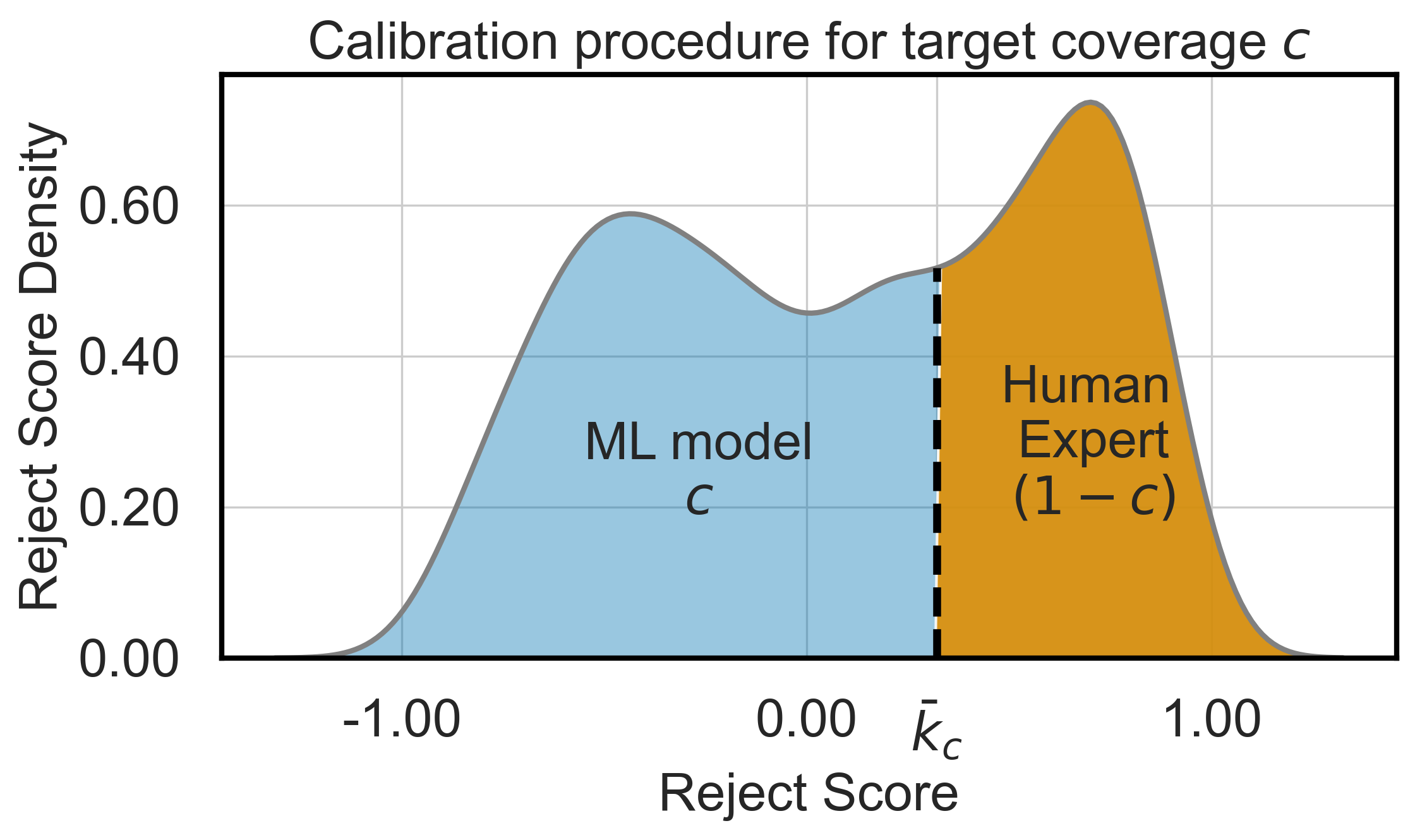
Most methods design the deferring strategy through a reject score function k:𝒳:𝑘𝒳k:\mathcal{X}\to\mathbb{R}, which estimates whether the human expert prediction is more likely to be correct than the one of the ML model [7]. High values of k(𝐱)𝑘𝐱k(\mathbf{x}) correspond to cases where the human expert is preferable, i.e., it is more likely to provide a correct prediction. Hence, we can set a threshold κ¯¯𝜅\overline{\kappa} over k(𝐱)𝑘𝐱k(\mathbf{x}) to define the policy function as g(𝐱)=𝟙{k(𝐱)κ¯}𝑔𝐱1𝑘𝐱¯𝜅g(\mathbf{x})=\mathds{1}\{k(\mathbf{x})\geq\overline{\kappa}\}. Okati et al. [2] show that such a thresholding strategy is optimal. In practice, one can estimate such a threshold in various ways. For instance, if there are no coverage constraints, a linear search procedure can be run by selecting the κ¯¯𝜅\overline{\kappa} that maximizes accuracy over a validation set [7]. Otherwise, one can consider a coverage-calibration procedure by setting κ¯¯𝜅\overline{\kappa} as the c𝑡ℎsuperscript𝑐𝑡ℎc^{\mathit{th}}-percentile of the reject score values over a validation set [20], as shown in Figure 3. In order to highlight the relationship between κ¯¯𝜅\overline{\kappa} and c𝑐c, we denote the estimated threshold for a target coverage c𝑐c as κ¯csubscript¯𝜅𝑐\overline{\kappa}_{c}, i.e., κ¯csubscript¯𝜅𝑐\overline{\kappa}_{c} is such that 𝔼[𝟙{k(𝐗)κ¯c}]=(1c)𝔼delimited-[]1𝑘𝐗subscript¯𝜅𝑐1𝑐\mathbb{E}[\mathds{1}\{k(\mathbf{X})\geq\overline{\kappa}_{c}\}]=(1-c).

2.3 Related work

By viewing the introduction of human-AI teams as an intervention in a ML-based or in a human-based decision flow, our work bridges causal inference for policy evaluation with deferring systems. To the best of our knowledge, the only related work is due to Choe et al. [21], who estimate the accuracy of abstaining classifiers (which do not account for deferring to human experts) on the abstained instances under the assumption that the abstention policy is stochastic. Such an assumption is impractical in the context of deferring systems. See Appendix A for additional related work.

Policy evaluation. Causal inference methods are commonly used to evaluate the effects of treatments/policies and, thus, inform policymakers [12]. Randomized control trials (RCT), i.e., experiments that assign units to treatment randomly, are the gold standard for inferring average causal effects (such as τ𝙰𝚃𝙴subscript𝜏𝙰𝚃𝙴\tau_{\mathtt{ATE}}) in many fields including healthcare [22], education [23], and finance [24]. When it is not possible to rely on RCTs, e.g., it is not ethical or too costly to run an experiment, one can resort to other techniques using observational data [11, 25]. The RD design has been used to assess the effectiveness of treatments in several fields, such as healthcare [26, 27, 28], criminal behavior [29], education [30, 31, 32, 33], public economics [34, 35, 36], and corporate finance [37].

Deferring systems applications. In recent years, deferring systems have been deployed to build human-AI teams in different settings. For instance, Van der Pias et al. [38] present a deferring system for sleep stage scoring, which can be used to allow physicians to focus on critical patients. Cianci et al. [39] adopt selective classification [40] for uncertainty self-assessment of a credit scoring ML model, with the purpose of informing the human decision maker. Bondi et al. [41] study a deferring system for evaluating the presence of animals in photo traps, showing that the performance of the deferring system is influenced by how the deferral choice is communicated to humans. We refer to Punzi et al. [42] for a recent survey on hybrid decision-making.

3 Evaluating deferring systems
Refer to caption
Figure 1: In blue, the (c)%percent𝑐({c})\% of instances (i.e., those with k(𝐱)<κ¯c𝑘𝐱subscript¯𝜅𝑐k(\mathbf{x})<\overline{\kappa}_{c}) assigned to the ML model; in orange, the (1c)%percent1𝑐(1-{c})\% instances (i.e., those with k(𝐱)κ¯c𝑘𝐱subscript¯𝜅𝑐k(\mathbf{x})\geq\overline{\kappa}_{c}) the human predicts.
Refer to caption
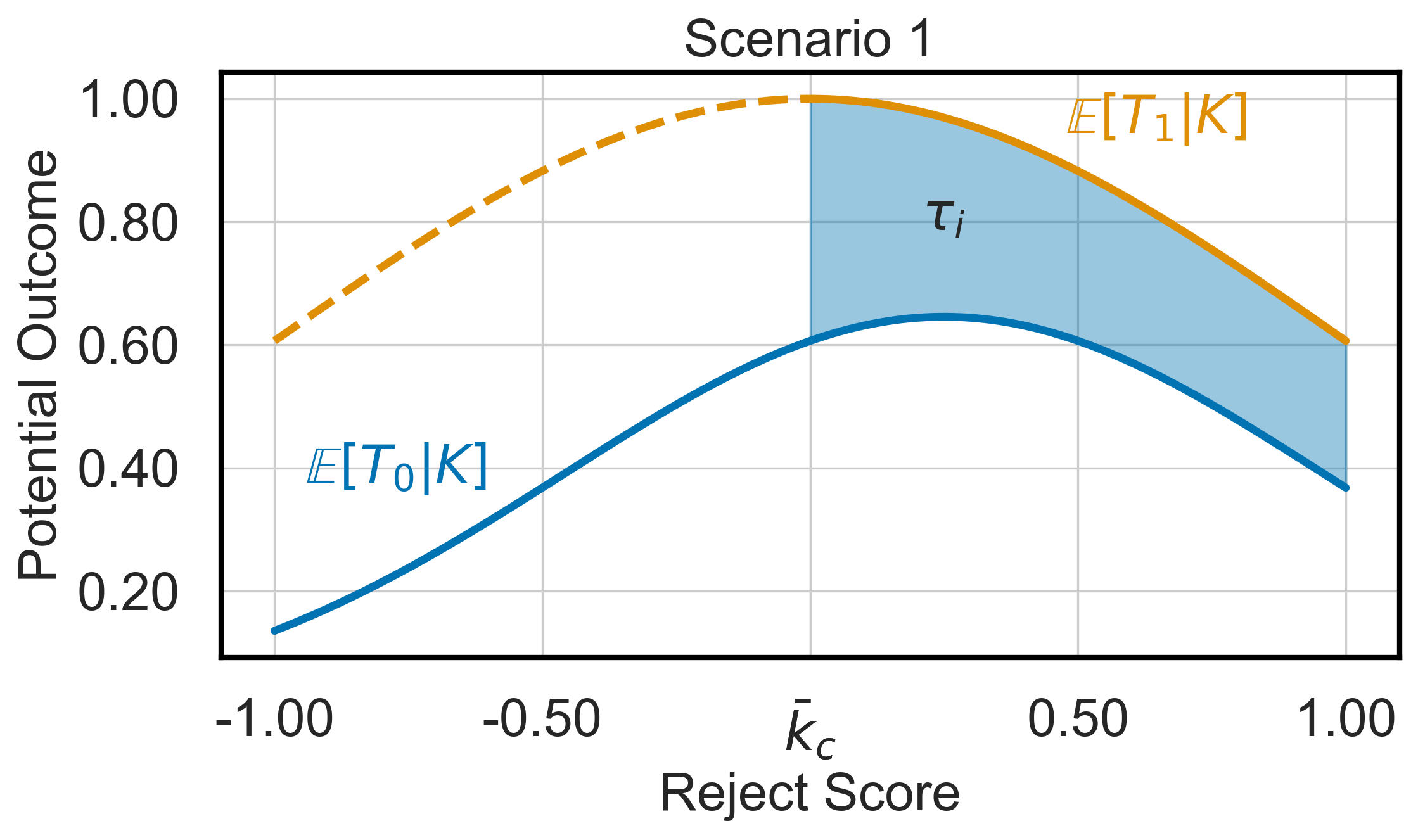
Figure 2: Scenario 1 assumptions: dashed lines are unobserved values and thick lines observed ones. The coloured area represents where the effects can be estimated (i.e., k(𝐱)κ¯c𝑘𝐱subscript¯𝜅𝑐k(\mathbf{x})\geq\overline{\kappa}_{c}).
Refer to caption
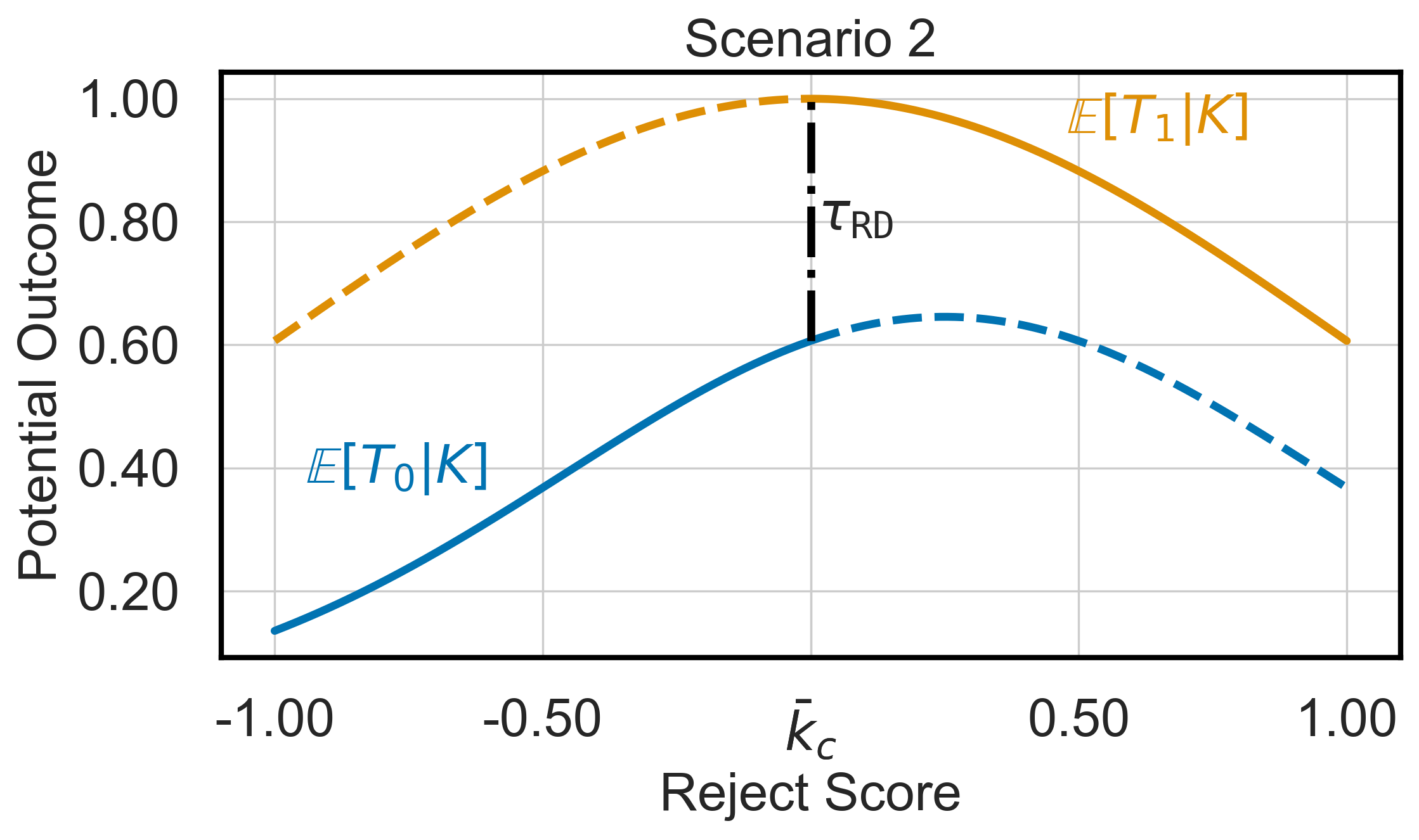
Figure 3: Scenario 2 assumptions: dashed lines are unobserved values and thick lines observed ones. We can estimate τ𝚁𝙳subscript𝜏𝚁𝙳\tau_{\mathtt{RD}} at the cutoff value (i.e., k(𝐱)=κ¯c𝑘𝐱subscript¯𝜅𝑐k(\mathbf{x})=\overline{\kappa}_{c}).

Problem statement. We consider the problem of measuring the causal contribution, in terms of accuracy, of deferring the prediction to a human expert in a given deferring system based on a reject score function. For this, we assume a given set of realizations 𝒟n={(𝐱i,yi)}i=1nsubscript𝒟𝑛superscriptsubscriptsubscript𝐱𝑖subscript𝑦𝑖𝑖1𝑛\mathcal{D}_{n}=\{(\mathbf{x}_{i},y_{i})\}_{i=1}^{n}, called a test set, of an i.i.d. random sample {(𝐗i,Yi)}i=1nsuperscriptsubscriptsubscript𝐗𝑖subscript𝑌𝑖𝑖1𝑛\{(\mathbf{X}_{i},Y_{i})\}_{i=1}^{n} over P(𝐗,Y)𝑃𝐗𝑌P(\mathbf{X},Y).

Table 1: Deferring systems under the Potential Outcome lens.
Potential Outcome Deferring Systems
running variable Visubscript𝑉𝑖V_{i} Kisubscript𝐾𝑖K_{i}
cutoff ξ𝜉\xi κ¯csubscript¯𝜅𝑐\overline{\kappa}_{c}
treatment Disubscript𝐷𝑖D_{i} Gisubscript𝐺𝑖G_{i}
outcome Oisubscript𝑂𝑖O_{i} Tisubscript𝑇𝑖T_{i}
potential outcomes Oi(d),d{0,1}subscript𝑂𝑖𝑑𝑑01O_{i}(d),d\in\{0,1\} Ti(g),g{0,1}subscript𝑇𝑖𝑔𝑔01T_{i}(g),g\in\{0,1\}
τisubscript𝜏𝑖\tau_{i} Oi(1)Oi(0)subscript𝑂𝑖1subscript𝑂𝑖0O_{i}(1)-O_{i}(0) Ti(1)Ti(0)subscript𝑇𝑖1subscript𝑇𝑖0T_{i}(1)-T_{i}(0)

Methodology. We tackle the problem above by bridging deferring systems with the potential outcome framework. The key observation is that the reject score maps to a running variable, and the accuracy of the ML model and of the human expert map to the potential outcomes.

Table 1 provides a mapping of the role of each variable of a deferring system into the potential outcomes framework. We have that: (i)𝑖(i) the reject score Ki=k(𝐗i)subscript𝐾𝑖𝑘subscript𝐗𝑖K_{i}=k(\mathbf{X}_{i}) is the running variable; (ii)𝑖𝑖(ii) the threshold κ¯c𝒦subscript¯𝜅𝑐𝒦\overline{\kappa}_{c}\in\mathcal{K} is the cutoff; (iii)𝑖𝑖𝑖(iii) the policy function Gi=𝟙{Kiκ¯c}subscript𝐺𝑖1subscript𝐾𝑖subscript¯𝜅𝑐G_{i}=\mathds{1}\{K_{i}\geq\overline{\kappa}_{c}\} is the treatment assignment: if Gi=1subscript𝐺𝑖1G_{i}=1, the human expert provides the prediction h(𝐗i)subscript𝐗𝑖h(\mathbf{X}_{i}), otherwise the ML model provides the prediction f(𝐗i)𝑓subscript𝐗𝑖f(\mathbf{X}_{i}); (iv)𝑖𝑣(iv) the outcome Ti=𝟙{ϑ(𝐗i)=Yi}subscript𝑇𝑖1italic-ϑsubscript𝐗𝑖subscript𝑌𝑖T_{i}=\mathds{1}\{\vartheta(\mathbf{X}_{i})=Y_{i}\} is an indicator function for whether the prediction of the deferring system is correct, i.e., the prediction equals the target variable Yisubscript𝑌𝑖Y_{i} or not; (v)𝑣(v) correctness of ML model Ti(0)=𝟙{f(𝐗i)=Yi}subscript𝑇𝑖01𝑓subscript𝐗𝑖subscript𝑌𝑖T_{i}(0)=\mathds{1}{}\{f(\mathbf{X}_{i})=Y_{i}\} and of the human expert Ti(1)=𝟙{h(𝐗i)=Yi}subscript𝑇𝑖11subscript𝐗𝑖subscript𝑌𝑖T_{i}(1)=\mathds{1}{}\{h(\mathbf{X}_{i})=Y_{i}\} are the potential outcomes, and they are connected to the outcome Tisubscript𝑇𝑖T_{i} as follows: Ti=GiTi(1)+(1Gi)Ti(0)subscript𝑇𝑖subscript𝐺𝑖subscript𝑇𝑖11subscript𝐺𝑖subscript𝑇𝑖0T_{i}=G_{i}\cdot T_{i}(1)+(1-G_{i})\cdot T_{i}(0); finally, (vi)𝑣𝑖(vi) the individual causal effect τisubscript𝜏𝑖\tau_{i} is the difference between Ti(1)subscript𝑇𝑖1T_{i}(1) and Ti(0)subscript𝑇𝑖0T_{i}(0).

In the following, we distinguish two scenarios, which allow for the identification of causal effects. In both scenarios, we assume that the human predictions h(𝐗i)subscript𝐗𝑖h(\mathbf{X}_{i}) can be accessed only for the deferred instances, i.e., if Gi=1subscript𝐺𝑖1G_{i}=1.

Scenario 1.

The ML model predictions f(𝐗i)𝑓subscript𝐗𝑖f(\mathbf{X}_{i}) can be accessed for the whole random sample.

This scenario covers cases in which the ML model can be called without any cost or side effects. For example, this is the case when the development team runs an internal evaluation of the deferring system. In this scenario, we can identify the causal effects of deferring to the human (Section 3.1). Example Ex1 from the introduction falls under this scenario.

Scenario 2.

The ML model predictions f(𝐗i)𝑓subscript𝐗𝑖f(\mathbf{X}_{i}) can be accessed only for the non-deferred instances, i.e., if Gi=0subscript𝐺𝑖0G_{i}=0.

This scenario covers cases in which model invocation is costly (e.g., due to a pay-per-use fee), may have side effects, or discloses sensitive data. For example, in an external audit, the owner of the deferring system may be reluctant to share ML predictions for deferred instances: since these predictions are not the system’s actual output, releasing them might not be legally binding. In this scenario, we can identify the causal effects of deferring to the human locally to the deferring threshold (Section 3.2). Moreover, this scenario is also able to cover the cases where the intervention to be causally evaluated is the introduction of the ML model in a fully human decision-making process, as in example Ex2 from the introduction. In example Ex2, we are not interested in the causal effect of deferring from the ML model to human expert, but rather of deferring from the human expert to the ML model. Therefore, Scenario 1 does not apply if we reverse the role of the ML model and the human expert, because we cannot assume to have the human expert decisions for cases assigned to the ML model. However, since the local causal effect of deferring from the human expert to the ML model is the opposite of the one of deferring from the ML model to the human expert, we can rely on Scenario 2 for estimating it.

3.1 Scenario 1: deferring systems as an almost perfect causal inference design

In this scenario, we are in the ideal situation in which both potential outcomes are observed for the deferred instances (Gi=1)G_{i}=1), as both the ML model prediction f(𝐗i)𝑓subscript𝐗𝑖f(\mathbf{X}_{i}), and the human prediction h(𝐗i)subscript𝐗𝑖h(\mathbf{X}_{i}), are available. Let n𝑛n be the size of the test set 𝒟nsubscript𝒟𝑛\mathcal{D}_{n}, then, the following holds.

Proposition 1.

Let Scenario 1 hold. Then, for each i[1,n]𝑖1𝑛i\in[1,n] such that Gi=1subscript𝐺𝑖1G_{i}=1:

τi=Ti(1)Ti(0)=𝟙{h(𝐗i)=Yi}𝟙{f(𝐗i)=Yi}.subscript𝜏𝑖subscript𝑇𝑖1subscript𝑇𝑖01subscript𝐗𝑖subscript𝑌𝑖1𝑓subscript𝐗𝑖subscript𝑌𝑖\tau_{i}=T_{i}(1)-T_{i}(0)=\mathds{1}\{h(\mathbf{X}_{i})=Y_{i}\}-\mathds{1}\{f(\mathbf{X}_{i})=Y_{i}\}.
Proof.

Identification is immediate because both potential outcomes are observed for a unit i[1,n]𝑖1𝑛i\in[1,n] that has also been evaluated by a human (Gi=1subscript𝐺𝑖1G_{i}=1). In particular, Ti(0)=𝟙{f(𝐗i)=Yi}subscript𝑇𝑖01𝑓subscript𝐗𝑖subscript𝑌𝑖T_{i}(0)=\mathds{1}\{f(\mathbf{X}_{i})=Y_{i}\} is observable because we are under Scenario 1 and Ti(1)=𝟙{h(𝐗i)=Yi})T_{i}(1)=\mathds{1}\{h(\mathbf{X}_{i})=Y_{i}\}) since Gi=1subscript𝐺𝑖1G_{i}=1. ∎

Because we can directly compute the most granular causal effect on deferred instances, τisubscript𝜏𝑖\tau_{i}, we can also retrieve less granular quantities. For instance, if we average the τisubscript𝜏𝑖\tau_{i} over the population of deferred units, we obtain the average treatment effect on the deferred, τ𝙰𝚃𝙳subscript𝜏𝙰𝚃𝙳\tau_{\mathtt{ATD}}, which is the deferring systems’ equivalent of τ𝙰𝚃𝚃subscript𝜏𝙰𝚃𝚃\tau_{\mathtt{ATT}} in (1). This causal estimand can be identified as follows.

Proposition 2.

Let Scenario 1 hold. Then:

τ𝙰𝚃𝙳=𝔼[T(1)T(0)|G=1]=𝔼[𝟙{h(𝐗)=Y}G=1]𝔼[𝟙{f(𝐗)=Y}G=1].subscript𝜏𝙰𝚃𝙳𝔼delimited-[]𝑇1conditional𝑇0𝐺1𝔼delimited-[]conditional1𝐗𝑌𝐺1𝔼delimited-[]conditional1𝑓𝐗𝑌𝐺1\tau_{\mathtt{ATD}}=\mathbb{E}[T(1)-T(0)|G=1]=\mathbb{E}\left[\mathds{1}\{h(\mathbf{X})=Y\}\mid G=1\right]-\mathbb{E}\left[\mathds{1}\{f(\mathbf{X})=Y\}\mid G=1\right].

The proof can be found in Appendix B. τ𝙰𝚃𝙳subscript𝜏𝙰𝚃𝙳\tau_{\mathtt{ATD}} allows us to measure the (average) effect on accuracy due to the “intervention” of deferring to a human the prediction for the deferred instances. Intuitively, τ𝙰𝚃𝙳subscript𝜏𝙰𝚃𝙳\tau_{\mathtt{ATD}} estimates what would be the average percentage increase in accuracy for deferred instances if the human predicts instead of the ML model. This effect motivates the introduction of a deferring system to stakeholders. Policymakers can use it to assess the impact of such systems. The estimation of τ𝙰𝚃𝙳subscript𝜏𝙰𝚃𝙳\tau_{\mathtt{ATD}} is straightforward and can be conducted via a simple difference-in-means estimator of the form:

τ^𝙰𝚃𝙳=1n1i[1,n]:g(𝐱i)=1[ti(1)ti(0)]=1n1i[1,n]:g(𝐱i)=1[𝟙{h(𝐱i)=yi}𝟙{f(𝐱i)=yi}],subscript^𝜏𝙰𝚃𝙳1subscript𝑛1subscript:𝑖1𝑛𝑔subscript𝐱𝑖1delimited-[]subscript𝑡𝑖1subscript𝑡𝑖01subscript𝑛1subscript:𝑖1𝑛𝑔subscript𝐱𝑖1delimited-[]1subscript𝐱𝑖subscript𝑦𝑖1𝑓subscript𝐱𝑖subscript𝑦𝑖\widehat{\tau}_{\mathtt{ATD}}=\frac{1}{n_{1}}\sum_{i\in[1,n]:g(\mathbf{x}_{i})=1}\left[t_{i}(1)-t_{i}(0)\right]=\frac{1}{n_{1}}\sum_{i\in[1,n]:g(\mathbf{x}_{i})=1}\left[\mathds{1}\{h(\mathbf{x}_{i})=y_{i}\}-\mathds{1}\{f(\mathbf{x}_{i})=y_{i}\}\right],

where n1:=|{i[1,n]:g(𝐱i)=1}|assignsubscript𝑛1conditional-set𝑖1𝑛𝑔subscript𝐱𝑖1n_{1}:=|\{i\in[1,n]:g(\mathbf{x}_{i})=1\}| is the number of deferred instances in the test set.

Furthermore, any aggregated metrics of the individual causal effects on the deferred can be estimated in this setting. Another interesting quantity is:

τ𝙰𝚃𝙳(k)=𝔼[T(1)T(0)G=1,K=k],kκ¯c,formulae-sequencesubscript𝜏𝙰𝚃𝙳𝑘𝔼delimited-[]formulae-sequence𝑇1conditional𝑇0𝐺1𝐾𝑘𝑘subscript¯𝜅𝑐\tau_{\mathtt{ATD}}(k)=\mathbb{E}[T(1)-T(0)\mid G=1,K=k],\qquad k\geq\overline{\kappa}_{c},

which measures how the average difference in predictive accuracy changes as the coverage varies above the threshold κ¯csubscript¯𝜅𝑐\overline{\kappa}_{c}. Notice that 𝔼[T(1)T(0)G=1,K=k]=𝔼[T(1)T(0)K=k]𝔼delimited-[]formulae-sequence𝑇1conditional𝑇0𝐺1𝐾𝑘𝔼delimited-[]𝑇1conditional𝑇0𝐾𝑘\mathbb{E}[T(1)-T(0)\mid G=1,K=k]=\mathbb{E}[T(1)-T(0)\mid K=k] since kκ¯c𝑘subscript¯𝜅𝑐k\geq\overline{\kappa}_{c} if and only if G=1𝐺1G=1. Given kκ¯c𝑘subscript¯𝜅𝑐k\geq\overline{\kappa}_{c}, a natural estimator of τ𝙰𝚃𝙳(k)subscript𝜏𝙰𝚃𝙳𝑘\tau_{\mathtt{ATD}}(k) would be a non-parametric local polynomial kernel regression around k𝑘k. Local polynomial kernel regressions [43] fit a p𝑝p-th order polynomial locally at k𝑘k via weighted least squares, where the weight of each instance is determined by the shape of the kernel and is non-increasing in the distance between k𝑘k and k(𝐱i)𝑘subscript𝐱𝑖k(\mathbf{x}_{i}).

3.2 Scenario 2: deferring systems as an RD design

If we cannot access the ML model predictions for the deferred instances, we can still exploit the additional knowledge on the policy function to estimate causal quantities. In particular, we can exploit the fact that deferring systems can be interpreted as an RD design to compute a local version of τ𝙰𝚃𝙳subscript𝜏𝙰𝚃𝙳\tau_{\mathtt{ATD}}. In this scenario, τ𝚁𝙳subscript𝜏𝚁𝙳\tau_{\mathtt{RD}} answers the following question: for a fixed coverage value c𝑐c and the corresponding reject score threshold κ¯csubscript¯𝜅𝑐\overline{\kappa}_{c}, what would be the increase in accuracy if we let the human expert predict instead of the ML model for the instances with reject score close to κ¯csubscript¯𝜅𝑐\overline{\kappa}_{c}? Such an interpretation is possible if Assumption 1 holds. If we have reasons to believe that small changes of the reject-score threshold κ¯csubscript¯𝜅𝑐\overline{\kappa}_{c} do not abruptly change the expected predictive accuracy of the human expert and of the ML model, then Assumption 1 is satisfied.

Proposition 3.

Let Scenario 2 hold and let Assumption 1 be satisfied for the deferring system. Then

limkκ¯c+𝔼[TK=k]limkκ¯c𝔼[TK=k]=τ𝚁𝙳,subscript𝑘superscriptsubscript¯𝜅𝑐𝔼delimited-[]conditional𝑇𝐾𝑘subscript𝑘superscriptsubscript¯𝜅𝑐𝔼delimited-[]conditional𝑇𝐾𝑘subscript𝜏𝚁𝙳\lim_{k\to\overline{\kappa}_{c}^{+}}\mathbb{E}[T\mid K=k]-\lim_{k\to\overline{\kappa}_{c}^{-}}\mathbb{E}[T\mid K=k]=\tau_{\mathtt{RD}},

where τ𝚁𝙳:=𝔼[T(1)T(0)K=κ¯c]assignsubscript𝜏𝚁𝙳𝔼delimited-[]𝑇1conditional𝑇0𝐾subscript¯𝜅𝑐\tau_{\mathtt{RD}}:=\mathbb{E}[T(1)-T(0)\mid K=\overline{\kappa}_{c}].

The proof can be found in Appendix B. Proposition 3 allows us to evaluate the causal effect of deferring to a human in a decision flow even if we do not have access to ML predictions for the deferred instances. Indeed, τ𝚁𝙳subscript𝜏𝚁𝙳\tau_{\mathtt{RD}} readily quantifies the gain in predictive accuracy of having the human expert predicting in place of the ML model at the cutoff. The local nature of τ𝚁𝙳subscript𝜏𝚁𝙳\tau_{\mathtt{RD}} motivates the use of local non-parametric polynomial kernel regression to estimate 𝔼[TK=κ¯c]𝔼delimited-[]conditional𝑇𝐾subscript¯𝜅𝑐\mathbb{E}[T\mid K=\overline{\kappa}_{c}] from the left and the right of the cutoff, thus obtaining an estimator τ^𝚁𝙳subscript^𝜏𝚁𝙳\hat{\tau}_{\mathtt{RD}} of τ𝚁𝙳subscript𝜏𝚁𝙳\tau_{\mathtt{RD}}. We point out that τ𝚁𝙳subscript𝜏𝚁𝙳\tau_{\mathtt{RD}} can also be computed under Scenario 1. In Appendix C, we discuss additional caveats, including how to set the optimal coverage, how to check if Assumption 1 holds, and the uncertainty due to the ML model estimation.

4 Experimental evaluation

We experimentally address three questions:

Q1: What causal effects of deferring can be estimated under Scenario 1 in a controlled setting?

Q2: What causal effects of deferring can be estimated under Scenario 2 in a controlled setting?

Q3: What are the causal effects of deferring on real datasets?

To address Q1 and Q2, we consider a simulated setting to control the data-generating process. We then address Q3 by considering real-world datasets, discussing in this section the results for Scenario 1. Complete results for synthetic and real data are reported in Appendix D.2. All experimental software is available at https://github.com/andrepugni/PODS. Experimental hardware specifications and carbon footprint are reported in Appendix D.1.4.

4.1 Experimental settings

Table 2: Datasets and baselines details (epochs - ep., learning rate - lr, optimizer - op.).
dataset n |𝓨|𝓨|\mathcal{Y}| human network model pre-trained used in hyper-parameters
synth 20k 2 synthetic linear no [7] ep.=50;lr=1e2;op.=Adamformulae-sequenceep.50formulae-sequencelr1𝑒2op.Adam\texttt{ep.}=50;\texttt{lr}=1e-2;\-\texttt{op.}=\texttt{Adam}
cifar10h 10k 10 separate annotator WideResNet [44] yes [7, 8] ep.=150;lr=1e3;op.=AdamWformulae-sequenceep.150formulae-sequencelr1𝑒3op.AdamW\texttt{ep.}=150;\texttt{lr}=1e-3;\-\texttt{op.}=\texttt{AdamW}
galaxyzoo 10k 2 random annotator ResNet50 [45] yes [2, 5, 7] ep.=50;lr=1e3;op.=Adamformulae-sequenceep.50formulae-sequencelr1𝑒3op.Adam\texttt{ep.}=50;\texttt{lr}=1e-3;\-\texttt{op.}=\texttt{Adam}
hatespeech 25k 3 random annotator FNN on SBERT embeddings [46] yes [2, 5, 7, 8] ep.=100;lr=1e2;op.=Adamformulae-sequenceep.100formulae-sequencelr1𝑒2op.Adam\texttt{ep.}=100;\texttt{lr}=1e-2;\-\texttt{op.}=\texttt{Adam}
xray-airspace 4.4k 2 random annotator DenseNet121 [47] yes [7] ep.=3;lr=1e3;op.=AdamWformulae-sequenceep.3formulae-sequencelr1𝑒3op.AdamW\texttt{ep.}=3;\texttt{lr}=1e-3;\-\texttt{op.}=\texttt{AdamW}

Data. For Q1 and Q2, we generate synthetic data using the procedure from Mozannar et al. [7]. Such a procedure generates samples containing (i) instances for which the human expert performs better than the ML model and (ii) instances for which the ML model is better than the human expert. Regarding Q3, we consider four datasets used in the LtD literature: cifar10h [48], a hard-labelled version of galaxyzoo [49], hatespeech [50], and xray-airspace [51, 52]. Table 2 provides relevant data characteristics, while the applied pre-processing is detailed in Appendix D.1.1.

Baselines. We consider several deferring systems, including: Selective Prediction (SP) [53], Compare Confidence (CC) [3], Differentiable Triage (DT) [2], Cross-Entropy Surrogate (LCE) [4], One Vs All (OVA) [5], Realizable Surrogate (RS) [7] and Asymmetric SoftMax (ASM) [8]. Table 2 reports the base network model and the methods’ hyper-parameters used for each dataset. We provide further details for the baselines and the hyper-parameters choice in Appendices D.1.2, D.1.3.

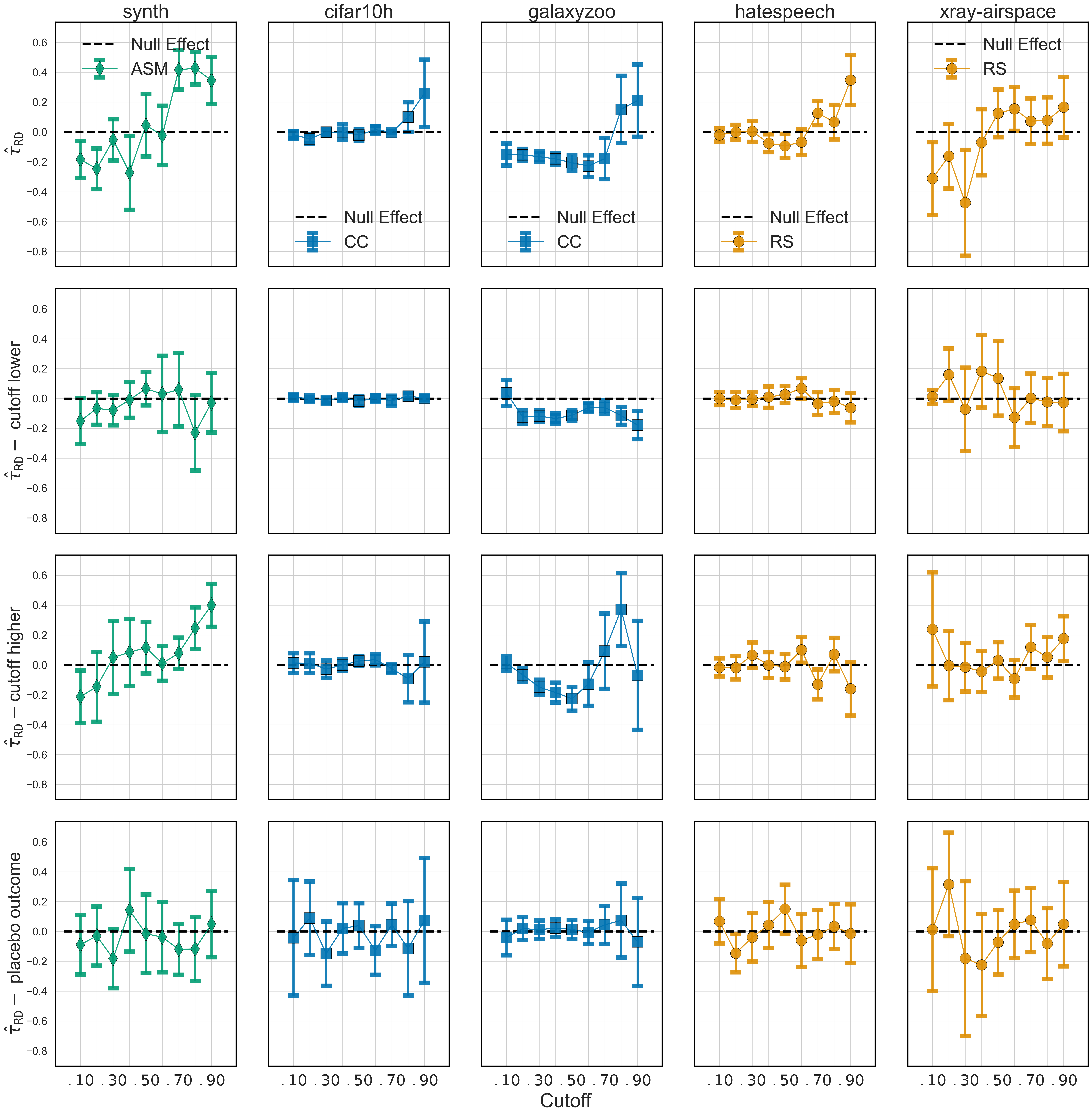
General setup. For all the experiments, we consider the following steps: (i)𝑖(i) we randomly split the dataset in training, validation, and test set, according to a 70%,10%,20%percent70percent10percent2070\%,10\%,20\% proportion; (ii)𝑖𝑖(ii) we train the deferring system on the training set; (iii)𝑖𝑖𝑖(iii) we estimate different cutoff values κ¯csubscript¯𝜅𝑐\overline{\kappa}_{c} over the validation set, considering each of the following target coverages c{.10,.20,.30,.40,.50,.60,.70,.80,.90}𝑐.10.20.30.40.50.60.70.80.90c\in\{.10,.20,.30,.40,.50,.60,.70,.80,.90\}; (iv)𝑖𝑣(iv) for each cutoff value κ¯csubscript¯𝜅𝑐\overline{\kappa}_{c}, we estimate on the test set the deferring system accuracy as well as τ𝙰𝚃𝙳subscript𝜏𝙰𝚃𝙳\tau_{\mathtt{ATD}} and τ𝚁𝙳subscript𝜏𝚁𝙳\tau_{\mathtt{RD}}. We consider a single training, validation, and test split since our goal is estimating the causal effect of implementing a deferring system, not estimating its predictive accuracy. The estimate τ^𝙰𝚃𝙳subscript^𝜏𝙰𝚃𝙳\hat{\tau}_{\mathtt{ATD}} is computed through a difference in means estimator and τ^𝚁𝙳subscript^𝜏𝚁𝙳\hat{\tau}_{\mathtt{RD}} is obtained using the default implementation of rdrobust package [54], i.e., a local linear kernel regression with optimal bandwidth [55]. To assess the statistical significance of the results, we report the 95% confidence intervals and the corresponding p𝑝p-values (pv𝑝𝑣pv) associated with τ^𝙰𝚃𝙳subscript^𝜏𝙰𝚃𝙳\hat{\tau}_{\mathtt{ATD}} and τ^𝚁𝙳subscript^𝜏𝚁𝙳\hat{\tau}_{\mathtt{RD}} when testing the null hypotheses of τ𝙰𝚃𝙳=0subscript𝜏𝙰𝚃𝙳0\tau_{\mathtt{ATD}}=0 and τ𝚁𝙳=0subscript𝜏𝚁𝙳0\tau_{\mathtt{RD}}=0, respectively. We correct for multiple testing through the Bonferroni correction for all the tested hypotheses (five datasets, ten coverages under Scenario 1 and nine under Scenario 2, seven methods): to achieve significance at a family-wise error rate of α=.05𝛼.05\alpha=.05, the p𝑝p-value must be smaller than 7.52e57.52E-57.5210-5.

4.2 Experimental results

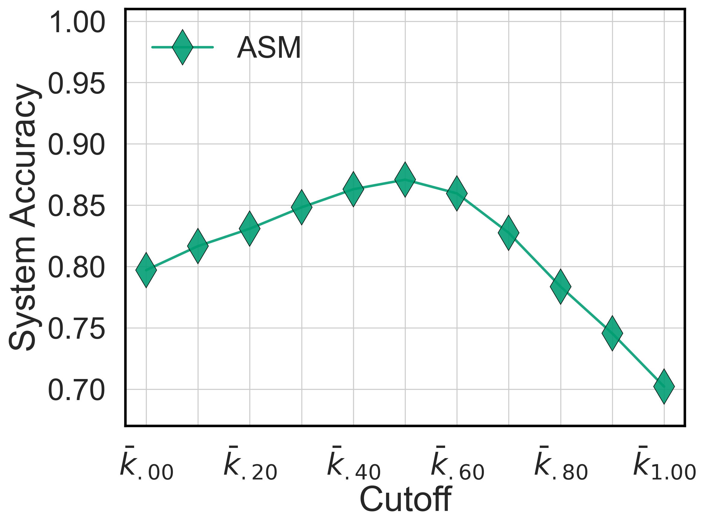
Figure 4 shows the results on the synthetic data (Q1 and Q2). Concerning real data (Q3), Figure 5 reports the results for Scenario 1, while results for Scenario 2 are discussed in Appendix D.2. For each dataset, we also report the best-deferring system in terms of accuracy: Figure 4(a) shows the accuracy for the synth dataset, while the bottom row of Figure 5 plots the accuracy for the real datasets. Appendix D.2 reports results for the other baselines.
Refer to caption
(a) ASM accuracy.
Refer to caption
(b) τ^𝙰𝚃𝙳subscript^𝜏𝙰𝚃𝙳\hat{\tau}_{\mathtt{ATD}} for ASM.
Refer to caption
(c) τ^𝙰𝚃𝙳subscript^𝜏𝙰𝚃𝙳\hat{\tau}_{\mathtt{ATD}} at c=.90𝑐.90c=.90.
Refer to caption
(d) τ^𝚁𝙳subscript^𝜏𝚁𝙳\hat{\tau}_{\mathtt{RD}} for ASM.
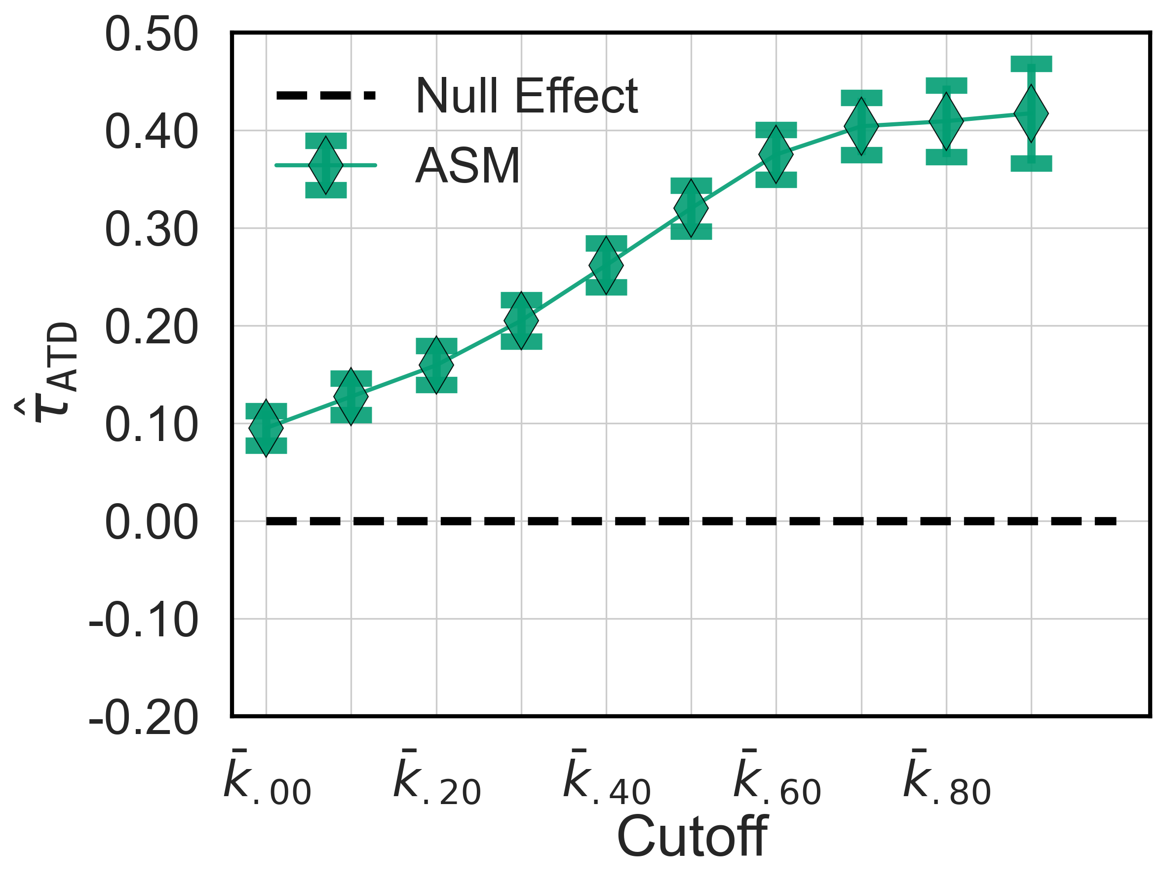
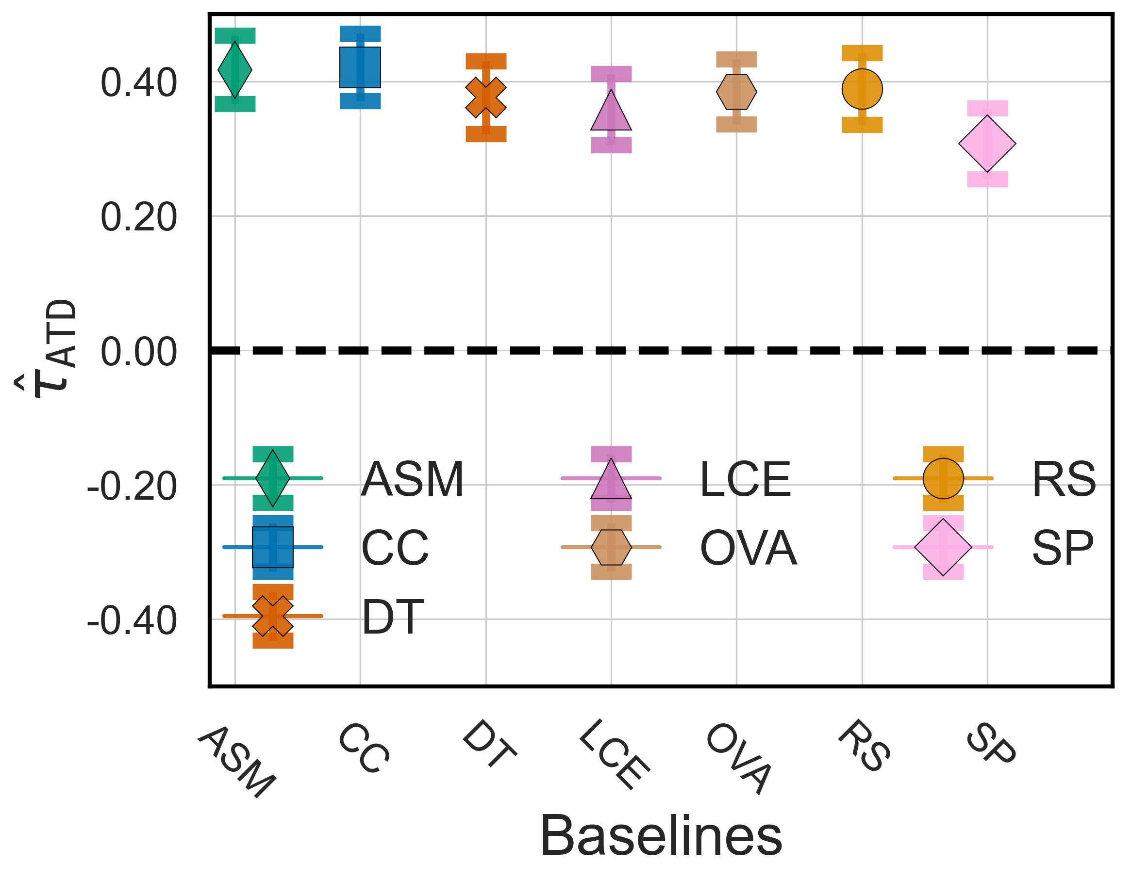
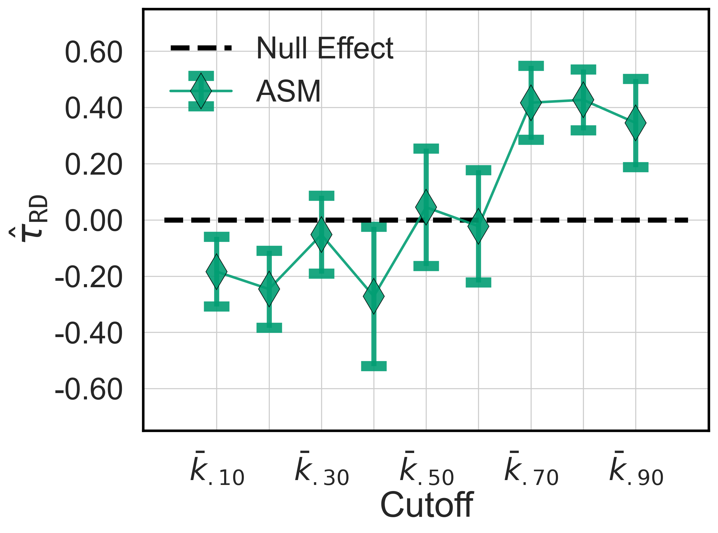
Figure 4: Performance on synthetic data. (a) reports the deferring system accuracy when varying cutoff κ¯csubscript¯𝜅𝑐\overline{\kappa}_{c} for the best baseline Asymmetric SoftMax (ASM) w.r.t. accuracy. (b) reports estimated τ^𝙰𝚃𝙳subscript^𝜏𝙰𝚃𝙳\hat{\tau}_{\mathtt{ATD}} when varying cutoff κ¯csubscript¯𝜅𝑐\overline{\kappa}_{c} on synthetic data for the best baseline. (c) compares the τ^𝙰𝚃𝙳subscript^𝜏𝙰𝚃𝙳\hat{\tau}_{\mathtt{ATD}} of multiple baselines at a fixed coverage c=.90𝑐.90c=.90. (d) reports estimated τ^𝚁𝙳subscript^𝜏𝚁𝙳\hat{\tau}_{\mathtt{RD}} when varying cutoff κ¯csubscript¯𝜅𝑐\overline{\kappa}_{c} for the best baseline.

Q1: causal effects under Scenario 1. Figure 4(b) shows the estimated τ^𝙰𝚃𝙳subscript^𝜏𝙰𝚃𝙳\hat{\tau}_{\mathtt{ATD}}s (the green diamonds) and their confidence intervals when varying the cutoff κ¯csubscript¯𝜅𝑐\overline{\kappa}_{c}. The black horizontal line denotes the null effects for τ^𝙰𝚃𝙳subscript^𝜏𝙰𝚃𝙳\hat{\tau}_{\mathtt{ATD}} and τ^𝚁𝙳subscript^𝜏𝚁𝙳\hat{\tau}_{\mathtt{RD}}. The plot confirms the effectiveness of ASM, with an increasing trend in the estimated causal effects, ranging from .095absent.095\approx.095 (pv6.98e26)𝑝𝑣6.98E-26(pv\approx$6.9810-26$) at zero coverage to .417absent.417\approx.417 (pv7.32e58𝑝𝑣7.32E-58pv\approx$7.3210-58$) at c=.90𝑐.90c=.90. Hence, introducing a deferring system turns out to be beneficial. Moreover, the strictly increasing value of τ^𝙰𝚃𝙳subscript^𝜏𝙰𝚃𝙳\hat{\tau}_{\mathtt{ATD}} w.r.t. the cutoff κ¯csubscript¯𝜅𝑐\overline{\kappa}_{c} allows us to confirm the deferring strategy’s effectiveness further. In fact, the higher the coverage, the more difficult instances are deferred to the human. Hence, the system is properly ranking the instances. We point out that this effect cannot be quantified by only examining the accuracy (see Figure 4(a)), as done by existing works in the literature.

Moreover, under Scenario 1, we can fix the target coverage and compare the estimate τ^𝙰𝚃𝙳subscript^𝜏𝙰𝚃𝙳\hat{\tau}_{\mathtt{ATD}} for multiple deferring systems. Figure 4(c) provides an example of this approach for c=.90𝑐.90c=.90. The ASM and CC baselines perform the best in such a case.

Q2: causal effects under Scenario 2. Due to the limited access to the ML model predictions, under Scenario 2, the estimation of the causal effect τ𝚁𝙳subscript𝜏𝚁𝙳\tau_{\mathtt{RD}} can be done only at the cutoff value κ¯csubscript¯𝜅𝑐\overline{\kappa}_{c} because (i)𝑖(i) we do not observe human predictions for the instances with reject-score below κ¯csubscript¯𝜅𝑐\overline{\kappa}_{{c}}; (ii)𝑖𝑖(ii) we cannot access the ML model predictions for the instances with reject score above κ¯csubscript¯𝜅𝑐\overline{\kappa}_{c}; and (iii)𝑖𝑖𝑖(iii) we cannot freely compare the performance on instances assigned to the ML model with performance on instances deferred to the expert as they are different from each other by construction. Figure 4(d) reports the estimated τ^𝚁𝙳subscript^𝜏𝚁𝙳\hat{\tau}_{\mathtt{RD}}’s: coefficients are negative (and not significant) for low coverage values, reaching the minimum value at κ¯.40subscript¯𝜅.40\overline{\kappa}_{.40} with an estimated effect of .272absent.272\approx-.272 (p𝑝p-value 3.14e2absent3.14E-2\approx$3.1410-2$). The estimates increase and become significant for larger coverage values, achieving a maximum value of .427absent.427\approx.427 (p𝑝p-value 1.20e14absent1.20E-14\approx$1.2010-14$) at c=.80𝑐.80c=.80. Thus, for the instances with a reject score value close to κ¯.80subscript¯𝜅.80\overline{\kappa}_{.80}, deferring to a human expert causes an increase in accuracy of 42.7%absentpercent42.7\approx 42.7\%.

As a general consideration, at the cutoff for which the estimated τ^𝚁𝙳subscript^𝜏𝚁𝙳\hat{\tau}_{\mathtt{RD}} is close to zero, we have that predicting with an ML model or a human expert is the same. Hence, such a cutoff maximizes the overall human-AI team accuracy. In higher cutoff values, the human performs better, while in lower cutoff values, the ML model performs better. From Figure 4(d), the τ^𝚁𝙳subscript^𝜏𝚁𝙳\hat{\tau}_{\mathtt{RD}} is close to zero for κ¯.50subscript¯𝜅.50\overline{\kappa}_{.50}. At such a cutoff, accuracy is maximized, as shown in Figure 4(a). In summary, the study of τ^𝚁𝙳subscript^𝜏𝚁𝙳\hat{\tau}_{\mathtt{RD}} at the variation of κ¯csubscript¯𝜅𝑐\overline{\kappa}_{c} helps evaluate whether the threshold κ¯¯𝜅\overline{\kappa} in the deferring system has been properly set.

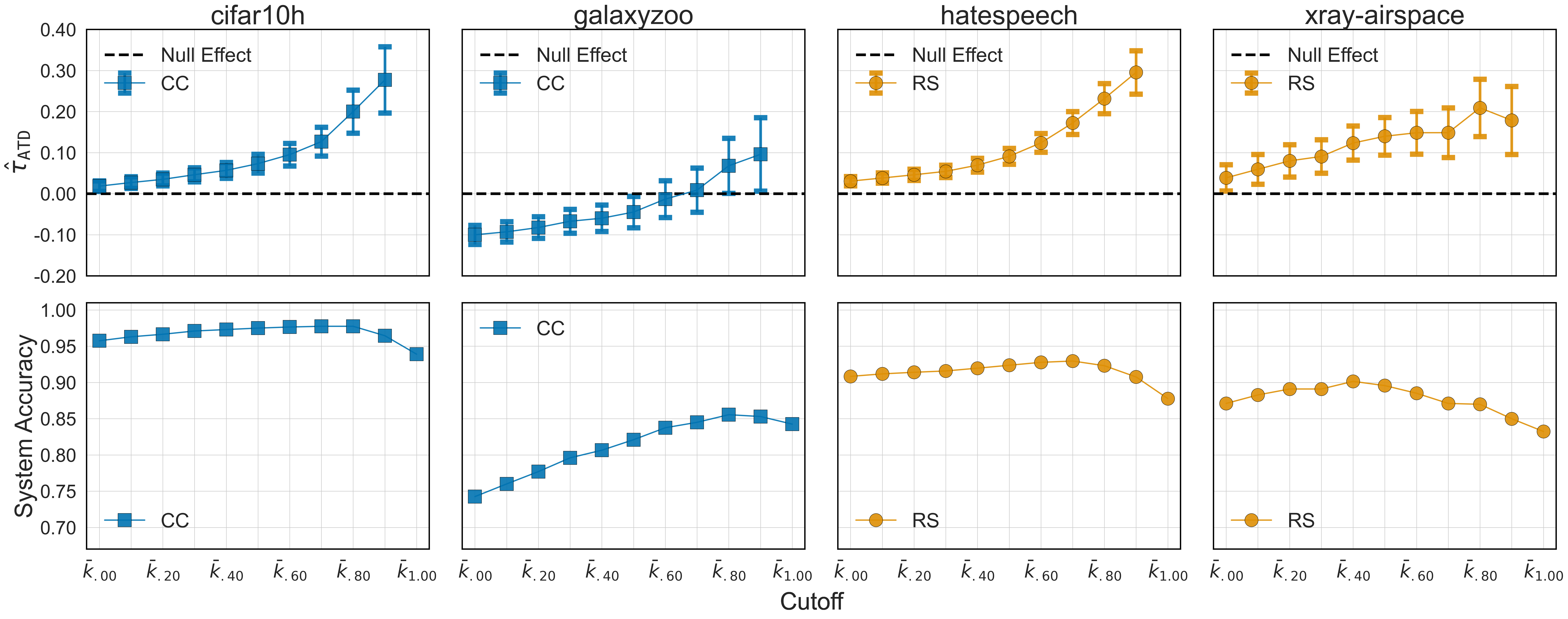
Q3: real datasets. Consider Figure 5. Regarding cifar10h, the τ^𝙰𝚃𝙳subscript^𝜏𝙰𝚃𝙳\hat{\tau}_{\mathtt{ATD}}’s are positive and increasing with κ¯csubscript¯𝜅𝑐\overline{\kappa}_{c}: the values range from .019absent.019\approx.019 at c=0𝑐0c=0 to .265absent.265\approx.265 (pv2.83e10)𝑝𝑣2.83E-10(pv\approx$2.8310-10$) at c=.90𝑐.90c=.90. This means that the deferring system correctly identifies those instances where the ML model is better than the human expert because deferring fewer instances yields higher τ^𝙰𝚃𝙳subscript^𝜏𝙰𝚃𝙳\hat{\tau}_{\mathtt{ATD}}’s.

For galaxyzoo, τ^𝙰𝚃𝙳subscript^𝜏𝙰𝚃𝙳\hat{\tau}_{\mathtt{ATD}} takes negative values for the coverages below c=.70𝑐.70c=.70. This is because the ML model at full coverage (accuracy of .843absent.843\approx.843) performs better than the human expert (accuracy of .743absent.743\approx.743). Moreover, for c=.80𝑐.80c=.80 and c=.90𝑐.90c=.90, the estimated τ^𝙰𝚃𝙳subscript^𝜏𝙰𝚃𝙳\hat{\tau}_{\mathtt{ATD}} are .068absent.068\approx.068 (pv4.69e2)𝑝𝑣4.69E-2(pv\approx$4.6910-2$) and .096absent.096\approx.096 (pv3.56e2)𝑝𝑣3.56E-2(pv\approx$3.5610-2$) respectively. In particular, they are not statistically different from zero. Hence, introducing a deferring system would not improve over a fully automated setting.

For hatespeech, the causal effects monotonically increase with the coverage, with τ^𝙰𝚃𝙳subscript^𝜏𝙰𝚃𝙳\hat{\tau}_{\mathtt{ATD}} ranging from .019absent.019\approx.019 (pv9.54e18)𝑝𝑣9.54E-18(pv\approx$9.5410-18$) at c=0𝑐0c=0 up to .295absent.295\approx.295 (pv7.40e28)𝑝𝑣7.40E-28(pv\approx$7.4010-28$) at c=.90𝑐.90c=.90. All the values significantly differ from zero, suggesting that deferring is effective.

We can also observe an overall positive effect for the xray-airspace dataset. Notice that the highest τ^𝙰𝚃𝙳subscript^𝜏𝙰𝚃𝙳\hat{\tau}_{\mathtt{ATD}} is achieved at c=.80𝑐.80c=.80 (.209absent.209\approx.209, pv4.29e9𝑝𝑣4.29E-9pv\approx$4.2910-9$), while the τ^𝙰𝚃𝙳subscript^𝜏𝙰𝚃𝙳\hat{\tau}_{\mathtt{ATD}} at c=.90𝑐.90c=.90 is lower (.179(\approx.179, pv2.41e5)pv\approx$2.4110-5$). This suggests that the reject score of the deferring system may not properly identify where the human expert performs better than the ML model. However, the difference between c=.80𝑐.80c=.80 and c=.90𝑐.90c=.90 is not statistically significant.

Refer to caption
Figure 5: Best deferring system performances on real data when varying the cutoff κ¯csubscript¯𝜅𝑐\overline{\kappa}_{c}. Top: estimated τ𝙰𝚃𝙳subscript𝜏𝙰𝚃𝙳\tau_{\mathtt{ATD}}. Bottom: accuracy. CC is Compare Confidence, RS is Realizable Surrogate.

5 Conclusions

We tackled the evaluation of predictive accuracy of deferring systems from a causal perspective. Our link with the potential outcomes and with the RD design frameworks directly allows for reasoning on the causal effects of the deferring strategy. Experiments showed some practical guidance on how to reason about the causal estimations to evaluate deferring systems.

Limitations and broader impact. We assumed that we had access to the reject scores k(𝐱)𝑘𝐱k(\mathbf{x}) of instances. This is not strictly required under Scenario 1, for which only the information on whether an instance is deferred or not is required. Conversely, identifying τ𝚁𝙳subscript𝜏𝚁𝙳\tau_{\mathtt{RD}} under Scenario 2 requires at least knowing the ranking induced by the reject score. Moreover, Assumption 1 must hold to identify τ𝚁𝙳subscript𝜏𝚁𝙳\tau_{\mathtt{RD}}. However, such an assumption is not directly verifiable and can only be falsified. We discuss this further in Appendix C and show how to falsify Assumption 1 in Appendix D.3.

From a broader impact perspective, our evaluation framework can be used to quantify the impact of deferring systems. Since these systems are becoming increasingly popular in many socially sensitive contexts, our approach can help better evaluate and deploy safer systems.

Future work. Multiple directions are open to future research. We mention extending our approach: to evaluate fairness metrics beyond predictive accuracy; to deferring strategies that consider multiple human experts; and to account for the influence that deferring has on human behaviour, as in strategic classification and performative predictions.

Acknowledgments

A. Pugnana and S. Ruggieri have received funding by PNRR - M4C2 - Investimento 1.3, Partenariato Esteso PE00000013 - “FAIR - Future Artificial Intelligence Research” - Spoke 1 “Human-centered AI”, funded by the European Commission under the NextGeneration EU programme. J. M. Alvarez and S. Ruggieri have received funding from the European Union’s Horizon 2020 research and innovation program under Marie Sklodowska-Curie Actions (grant agreement number 860630) for the project “NoBIAS - Artificial Intelligence without Bias”. This work reflects only the authors’ views and the European Research Executive Agency is not responsible for any use that may be made of the information it contains.

References

  • Madras et al. [2018] David Madras, Toniann Pitassi, and Richard S. Zemel. Predict responsibly: Improving fairness and accuracy by learning to defer. In NeurIPS, pages 6150–6160, 2018.
  • Okati et al. [2021] Nastaran Okati, Abir De, and Manuel Gomez-Rodriguez. Differentiable learning under triage. In NeurIPS, pages 9140–9151, 2021.
  • Raghu et al. [2019] Maithra Raghu, Katy Blumer, Greg Corrado, Jon M. Kleinberg, Ziad Obermeyer, and Sendhil Mullainathan. The algorithmic automation problem: Prediction, triage, and human effort. CoRR, abs/1903.12220, 2019.
  • Mozannar and Sontag [2020] Hussein Mozannar and David A. Sontag. Consistent estimators for learning to defer to an expert. In ICML, volume 119, pages 7076–7087. PMLR, 2020.
  • Verma and Nalisnick [2022] Rajeev Verma and Eric T. Nalisnick. Calibrated learning to defer with one-vs-all classifiers. In ICML, volume 162 of Proceedings of Machine Learning Research, pages 22184–22202. PMLR, 2022.
  • Verma et al. [2023] Rajeev Verma, Daniel Barrejón, and Eric T. Nalisnick. Learning to defer to multiple experts: Consistent surrogate losses, confidence calibration, and conformal ensembles. In AISTATS, volume 206, pages 11415–11434. PMLR, 2023.
  • Mozannar et al. [2023] Hussein Mozannar, Hunter Lang, Dennis Wei, Prasanna Sattigeri, Subhro Das, and David A. Sontag. Who should predict? exact algorithms for learning to defer to humans. In AISTATS, volume 206, pages 10520–10545. PMLR, 2023.
  • Cao et al. [2023] Yuzhou Cao, Hussein Mozannar, Lei Feng, Hongxin Wei, and Bo An. In defense of softmax parametrization for calibrated and consistent learning to defer. In NeurIPS, 2023.
  • Álvarez et al. [2024] José M. Álvarez, Alejandra Bringas-Colmenarejo, Alaa Elobaid, Simone Fabbrizzi, Miriam Fahimi, Antonio Ferrara, Siamak Ghodsi, Carlos Mougan, Ioanna Papageorgiou, Paula Reyero Lobo, Mayra Russo, Kristen M. Scott, Laura State, Xuan Zhao, and Salvatore Ruggieri. Policy advice and best practices on bias and fairness in AI. Ethics Inf. Technol., 26(2):31, 2024.
  • Pearl [2009] Judea Pearl. Causality: Models, Reasoning, and Inference. Cambridge University Press, 2009.
  • Nogueira et al. [2022] Ana Rita Nogueira, Andrea Pugnana, Salvatore Ruggieri, Dino Pedreschi, and João Gama. Methods and tools for causal discovery and causal inference. WIREs Data Mining Knowl. Discov., 12(2), 2022.
  • Abadie and Cattaneo [2018] Alberto Abadie and Matias D. Cattaneo. Econometric Methods for Program Evaluation. Annual Review of Economics, 10(1):465–503, 2018.
  • Neyman [1923] Jersey Neyman. Sur les applications de la théorie des probabilités aux experiences agricoles: Essai des principes. Roczniki Nauk Rolniczych, 10(1):1–51, 1923.
  • Rubin [1974] Donald B. Rubin. Estimating causal effects of treatments in randomized and nonrandomized studies. Journal of Educational Psychology, 66(5):688–701, October 1974.
  • Thistlethwaite and Campbell [1960a] Donald L Thistlethwaite and Donald T Campbell. Regression-discontinuity analysis: An alternative to the ex post facto experiment. Journal of Educational Psychology, 51(6):309, 1960a.
  • Rubin [1978] Donald B. Rubin. Bayesian Inference for Causal Effects: The Role of Randomization. The Annals of Statistics, 6(1):34–58, 1978.
  • Holland [1986] Paul W. Holland. Statistics and Causal Inference. Journal of the American Statistical Association, 81(396):945–960, December 1986.
  • Hahn et al. [2001] Jinyong Hahn, Petra Todd, and Wilbert Van der Klaauw. Identification and Estimation of Treatment Effects with a Regression-Discontinuity Design. Econometrica, 69(1):201–209, 2001.
  • Mao et al. [2023] Anqi Mao, Christopher Mohri, Mehryar Mohri, and Yutao Zhong. Two-stage learning to defer with multiple experts. In NeurIPS, 2023.
  • Pugnana et al. [2024] Andrea Pugnana, Lorenzo Perini, Jesse Davis, and Salvatore Ruggieri. Deep neural network benchmarks for selective classification. CoRR, abs/2401.12708, 2024.
  • Choe et al. [2023] Yo Joong Choe, Aditya Gangrade, and Aaditya Ramdas. Counterfactually comparing abstaining classifiers. In NeurIPS, 2023.
  • Stolberg et al. [2004] Harald O Stolberg, Geoffrey Norman, and Isabelle Trop. Randomized controlled trials. American Journal of Roentgenology, 183(6):1539–1544, 2004.
  • Carlana et al. [2022] Michela Carlana, Eliana La Ferrara, and Paolo Pinotti. Goals and gaps: Educational careers of immigrant children. Econometrica, 90(1):1–29, 2022.
  • Banerjee et al. [2015] Abhijit Banerjee, Esther Duflo, Rachel Glennerster, and Cynthia Kinnan. The miracle of microfinance? Evidence from a randomized evaluation. American Economic Journal: Applied Economics, pages 22–53, 2015.
  • Angrist and Pischke [2009] Joshua Angrist and Jörn-Steffen Pischke. Mostly Harmless Econometrics. Princeton University Press, 2009.
  • Ludwig and Miller [2007] Jens Ludwig and Douglas L. Miller. Does Head Start Improve Children’s Life Chances? Evidence from a Regression Discontinuity Design. The Quarterly Journal of Economics, 122(1):159–208, February 2007.
  • Boon et al. [2021] Michele Hilton Boon, Peter Craig, Hilary Thomson, Mhairi Campbell, and Laurence Moore. Regression discontinuity designs in health: a systematic review. Epidemiology, 32(1):87–93, 2021.
  • Cattaneo et al. [2023] Matias D Cattaneo, Luke Keele, and Rocío Titiunik. A guide to regression discontinuity designs in medical applications. Statistics in Medicine, 42(24):4484–4513, 2023.
  • Pinotti [2017] Paolo Pinotti. Clicking on Heaven’s Door: The Effect of Immigrant Legalization on Crime. American Economic Review, 107(1):138–168, January 2017.
  • Angrist and Lavy [1999] Joshua D. Angrist and Victor Lavy. Using Maimonides’ Rule to Estimate the Effect of Class Size on Scholastic Achievement. The Quarterly Journal of Economics, 114(2):533–575, May 1999.
  • Cellini et al. [2010] Stephanie Riegg Cellini, Fernando Ferreira, and Jesse Rothstein. The Value of School Facility Investments: Evidence from a Dynamic Regression Discontinuity Design. The Quarterly Journal of Economics, 125(1):215–261, 2010.
  • Duflo et al. [2011] Esther Duflo, Pascaline Dupas, and Michael Kremer. Peer Effects, Teacher Incentives, and the Impact of Tracking: Evidence from a Randomized Evaluation in Kenya. American Economic Review, 101(5):1739–1774, August 2011.
  • Pop-Eleches and Urquiola [2013] Cristian Pop-Eleches and Miguel Urquiola. Going to a Better School: Effects and Behavioral Responses. American Economic Review, 103(4):1289–1324, June 2013.
  • Lalive [2008] Rafael Lalive. How do extended benefits affect unemployment duration? A regression discontinuity approach. Journal of Econometrics, 142(2):785–806, February 2008.
  • Battistin et al. [2009] Erich Battistin, Agar Brugiavini, Enrico Rettore, and Guglielmo Weber. The Retirement Consumption Puzzle: Evidence from a Regression Discontinuity Approach. American Economic Review, 99(5):2209–2226, December 2009.
  • Coviello and Mariniello [2014] Decio Coviello and Mario Mariniello. Publicity requirements in public procurement: Evidence from a regression discontinuity design. Journal of Public Economics, 109:76–100, January 2014.
  • Flammer [2015] Caroline Flammer. Does Corporate Social Responsibility Lead to Superior Financial Performance? A Regression Discontinuity Approach. Management Science, 61(11):2549–2568, November 2015.
  • Van der Pias et al. [2023a] Dries Van der Pias, Wannes Meert, Johan Verbraecken, and Jesse Davis. A novel reject option applied to sleep stage scoring. In SDM, pages 820–828. SIAM, 2023a.
  • Cianci et al. [2023] Giuseppe Cianci, Roberto Goglia, Riccardo Guidotti, Matteo Kapllaj, Roberto Mosca, Andrea Pugnana, Franco Ricotti, and Salvatore Ruggieri. Applied data science for leasing score prediction. In IEEE Big Data, pages 1687–1696. IEEE, 2023.
  • El-Yaniv and Wiener [2010] Ran El-Yaniv and Yair Wiener. On the foundations of noise-free selective classification. J. Mach. Learn. Res., 11:1605–1641, 2010.
  • Bondi et al. [2022] Elizabeth Bondi, Raphael Koster, Hannah Sheahan, Martin J. Chadwick, Yoram Bachrach, A. Taylan Cemgil, Ulrich Paquet, and Krishnamurthy Dvijotham. Role of human-AI interaction in selective prediction. In AAAI, pages 5286–5294. AAAI Press, 2022.
  • Punzi et al. [2024] Clara Punzi, Roberto Pellungrini, Mattia Setzu, Fosca Giannotti, and Dino Pedreschi. AI, Meet Human: Learning paradigms for hybrid decision making systems. arXiv preprint arXiv:2402.06287, 2024.
  • Fan and Gijbels [1996] Jianqing Fan and Irène Gijbels. Local Polynomial Modelling and Its Applications: Monographs on Statistics and Applied Probability 66. Routledge, January 1996.
  • Zagoruyko and Komodakis [2016] Sergey Zagoruyko and Nikos Komodakis. Wide residual networks. In BMVC. BMVA Press, 2016.
  • He et al. [2016] Kaiming He, Xiangyu Zhang, Shaoqing Ren, and Jian Sun. Deep residual learning for image recognition. In CVPR, pages 770–778. IEEE Computer Society, 2016.
  • Reimers and Gurevych [2019] Nils Reimers and Iryna Gurevych. Sentence-bert: Sentence embeddings using siamese bert-networks. In EMNLP/IJCNLP (1), pages 3980–3990. Association for Computational Linguistics, 2019.
  • Huang et al. [2017] Gao Huang, Zhuang Liu, Laurens van der Maaten, and Kilian Q. Weinberger. Densely connected convolutional networks. In CVPR, pages 2261–2269. IEEE Computer Society, 2017.
  • Battleday et al. [2020] Ruairidh M. Battleday, Joshua C. Peterson, and Thomas L. Griffiths. Capturing human categorization of natural images at scale by combining deep networks and cognitive models. Nature communications, 11(1):5418, 2020.
  • AstroDave et al. [2013] AstroDave, AstroTom, Christopher Read @ Winton, joycenv, and Kyle Willett. Galaxy zoo - the galaxy challenge, 2013. URL https://kaggle.com/competitions/galaxy-zoo-the-galaxy-challenge.
  • Davidson et al. [2017] Thomas Davidson, Dana Warmsley, Michael W. Macy, and Ingmar Weber. Automated hate speech detection and the problem of offensive language. In ICWSM, pages 512–515. AAAI Press, 2017.
  • Wang et al. [2017] Xiaosong Wang, Yifan Peng, Le Lu, Zhiyong Lu, Mohammadhadi Bagheri, and Ronald M. Summers. Chestx-ray8: Hospital-scale chest x-ray database and benchmarks on weakly-supervised classification and localization of common thorax diseases. In CVPR, pages 3462–3471. IEEE Computer Society, 2017.
  • Majkowska et al. [2020] Anna Majkowska, Sid Mittal, David F Steiner, Joshua J Reicher, Scott Mayer McKinney, Gavin E Duggan, Krish Eswaran, Po-Hsuan Cameron Chen, Yun Liu, Sreenivasa Raju Kalidindi, et al. Chest radiograph interpretation with deep learning models: assessment with radiologist-adjudicated reference standards and population-adjusted evaluation. Radiology, 294(2):421–431, 2020.
  • Geifman and El-Yaniv [2017] Yonatan Geifman and Ran El-Yaniv. Selective classification for deep neural networks. In NIPS, pages 4878–4887, 2017.
  • Calonico et al. [2017] Sebastian Calonico, Matias D. Cattaneo, Max H. Farrell, and Rocio Titiunik. Rdrobust: Software for regression-discontinuity designs. The Stata Journal, 17(2):372–404, 2017.
  • Calonico et al. [2020] Sebastian Calonico, Matias D Cattaneo, and Max H Farrell. Optimal bandwidth choice for robust bias-corrected inference in regression discontinuity designs. The Econometrics Journal, 23(2):192–210, 2020.
  • Chow [1970] C. K. Chow. On optimum recognition error and reject tradeoff. IEEE Trans. Inf. Theory, 16(1):41–46, 1970.
  • Hendrickx et al. [2024] Kilian Hendrickx, Lorenzo Perini, Dries Van der Plas, Wannes Meert, and Jesse Davis. Machine learning with a reject option: a survey. Mach. Learn., 113(5):3073–3110, 2024.
  • Nalisnick et al. [2019] Eric T. Nalisnick, Akihiro Matsukawa, Yee Whye Teh, Dilan Görür, and Balaji Lakshminarayanan. Hybrid models with deep and invertible features. In ICML, volume 97, pages 4723–4732. PMLR, 2019.
  • Wang and Yiu [2020] Xin Wang and Siu-Ming Yiu. Classification with rejection: Scaling generative classifiers with supervised deep infomax. In IJCAI, pages 2980–2986. ijcai.org, 2020.
  • Coenen et al. [2020] Lize Coenen, Ahmed K. A. Abdullah, and Tias Guns. Probability of default estimation, with a reject option. In DSAA, pages 439–448. IEEE, 2020.
  • Liang et al. [2018] Shiyu Liang, Yixuan Li, and R. Srikant. Enhancing the reliability of out-of-distribution image detection in neural networks. In ICLR. OpenReview.net, 2018.
  • Kühne et al. [2021] Joana Kühne, Christian März, et al. Securing deep learning models with autoencoder based anomaly detection. In PHM Society European Conference, volume 6, pages 221–233, 2021.
  • Perini and Davis [2023] Lorenzo Perini and Jesse Davis. Unsupervised anomaly detection with rejection. In NeurIPS, 2023.
  • Van der Pias et al. [2023b] Dries Van der Pias, Wannes Meert, Johan Verbraecken, and Jesse Davis. A novel reject option applied to sleep stage scoring. In SDM, pages 820–828. SIAM, 2023b.
  • Cortes et al. [2023] Corinna Cortes, Giulia DeSalvo, and Mehryar Mohri. Theory and algorithms for learning with rejection in binary classification. Annals of Mathematics and Artificial Intelligence, pages 1–39, 2023.
  • Herbei and Wegkamp [2006] Radu Herbei and Maten H. Wegkamp. Classification with reject option. Can. J. Stat., 34(4):709––721, 2006.
  • Cortes et al. [2016] Corinna Cortes, Giulia DeSalvo, and Mehryar Mohri. Boosting with abstention. In NeurIPS, pages 1660–1668, 2016.
  • Tortorella [2005] Francesco Tortorella. A ROC-based reject rule for dichotomizers. Pattern Recognit. Lett., 26(2):167–180, 2005.
  • Condessa et al. [2013] Filipe Condessa, José M. Bioucas-Dias, Carlos A. Castro, John A. Ozolek, and Jelena Kovacevic. Classification with reject option using contextual information. In ISBI, pages 1340–1343. IEEE, 2013.
  • Franc et al. [2023] Vojtech Franc, Daniel Průša, and Václav Vorácek. Optimal strategies for reject option classifiers. J. Mach. Learn. Res., 24:11:1–11:49, 2023.
  • Denis and Hebiri [2020] Christophe Denis and Mohamed Hebiri. Consistency of plug-in confidence sets for classification in semi-supervised learning. J. of Nonpar. Statistics, 32(1):42–72, 2020.
  • Pugnana and Ruggieri [2023a] Andrea Pugnana and Salvatore Ruggieri. A model-agnostic heuristics for selective classification. In AAAI, pages 9461–9469. AAAI Press, 2023a.
  • Pugnana and Ruggieri [2023b] Andrea Pugnana and Salvatore Ruggieri. AUC-based selective classification. In AISTATS, volume 206, pages 2494–2514. PMLR, 2023b.
  • Geifman and El-Yaniv [2019] Yonatan Geifman and Ran El-Yaniv. Selectivenet: A deep neural network with an integrated reject option. In ICML, volume 97, pages 2151–2159. PMLR, 2019.
  • Corbière et al. [2019] Charles Corbière, Nicolas Thome, Avner Bar-Hen, Matthieu Cord, and Patrick Pérez. Addressing failure prediction by learning model confidence. In NeurIPS, pages 2898–2909, 2019.
  • Huang et al. [2020] Lang Huang, Chao Zhang, and Hongyang Zhang. Self-adaptive training: beyond empirical risk minimization. In NeurIPS, 2020.
  • Feng et al. [2023] Leo Feng, Mohamed Osama Ahmed, Hossein Hajimirsadeghi, and Amir H. Abdi. Towards better selective classification. In ICLR. OpenReview.net, 2023.
  • Chernozhukov et al. [2018] Victor Chernozhukov, Denis Chetverikov, Mert Demirer, Esther Duflo, Christian Hansen, Whitney Newey, and James Robins. Double/debiased machine learning for treatment and structural parameters. The Econometrics Journal, 21(1):C1–C68, February 2018.
  • De et al. [2020] Abir De, Paramita Koley, Niloy Ganguly, and Manuel Gomez-Rodriguez. Regression under human assistance. In AAAI, pages 2611–2620. AAAI Press, 2020.
  • De et al. [2021] Abir De, Nastaran Okati, Ali Zarezade, and Manuel Gomez Rodriguez. Classification under human assistance. In AAAI, pages 5905–5913. AAAI Press, 2021.
  • Thistlethwaite and Campbell [1960b] Donald L. Thistlethwaite and Donald T. Campbell. Regression-discontinuity analysis: An alternative to the ex post facto experiment. Journal of Educational Psychology, 51(6):309–317, 1960b.
  • Lee [2008] David S. Lee. Randomized experiments from non-random selection in U.S. House elections. Journal of Econometrics, 142(2):675–697, February 2008.
  • Cattaneo et al. [2015] Matias D. Cattaneo, Brigham R. Frandsen, and Rocío Titiunik. Randomization Inference in the Regression Discontinuity Design: An Application to Party Advantages in the U.S. Senate. Journal of Causal Inference, 3(1):1–24, March 2015.
  • Imbens and Angrist [1994] Guido W. Imbens and Joshua D. Angrist. Identification and Estimation of Local Average Treatment Effects. Econometrica, 62(2):467, March 1994.
  • Lee and Lemieux [2010] David S. Lee and Thomas Lemieux. Regression discontinuity designs in economics. Journal of economic literature, 48(2):281–355, 2010.
  • Cattaneo and Titiunik [2022] Matias D. Cattaneo and Rocío Titiunik. Regression Discontinuity Designs. Annual Review of Economics, 14(1):821–851, 2022.
  • Calonico et al. [2014] Sebastian Calonico, Matias D. Cattaneo, and Rocio Titiunik. Robust Nonparametric Confidence Intervals for Regression-Discontinuity Designs. Econometrica, 82(6):2295–2326, 2014.
  • Kolesár and Rothe [2018] Michal Kolesár and Christoph Rothe. Inference in Regression Discontinuity Designs with a Discrete Running Variable. American Economic Review, 108(8):2277–2304, August 2018.
  • Calonico et al. [2018] Sebastian Calonico, Matias D. Cattaneo, and Max H. Farrell. On the Effect of Bias Estimation on Coverage Accuracy in Nonparametric Inference. Journal of the American Statistical Association, 113(522):767–779, April 2018.
  • Calonico et al. [2022] Sebastian Calonico, Matias D. Cattaneo, and Max H. Farrell. Coverage error optimal confidence intervals for local polynomial regression. Bernoulli, 28(4), November 2022.
  • Cattaneo et al. [2019] Matias D. Cattaneo, Nicolás Idrobo, and Rocío Titiunik. A Practical Introduction to Regression Discontinuity Designs: Foundations. Cambridge University Press, 1 edition, November 2019.
  • Cattaneo et al. [2020] Matias D. Cattaneo, Michael Jansson, and Xinwei Ma. Simple Local Polynomial Density Estimators. Journal of the American Statistical Association, 115(531):1449–1455, July 2020.
  • Cattaneo et al. [2016] Matias D. Cattaneo, Luke Keele, Rocío Titiunik, and Gonzalo Vazquez-Bare. Interpreting Regression Discontinuity Designs with Multiple Cutoffs. The Journal of Politics, 78(4):1229–1248, October 2016.
  • Cattaneo et al. [2021] Matias D. Cattaneo, Luke Keele, Rocío Titiunik, and Gonzalo Vazquez-Bare. Extrapolating Treatment Effects in Multi-Cutoff Regression Discontinuity Designs. Journal of the American Statistical Association, 116(536):1941–1952, October 2021.
  • Dong and Lewbel [2015] Yingying Dong and Arthur Lewbel. Identifying the Effect of Changing the Policy Threshold in Regression Discontinuity Models. Review of Economics and Statistics, 97(5):1081–1092, December 2015.
  • Brown et al. [2020] Tom B. Brown, Benjamin Mann, Nick Ryder, Melanie Subbiah, Jared Kaplan, Prafulla Dhariwal, Arvind Neelakantan, Pranav Shyam, Girish Sastry, Amanda Askell, Sandhini Agarwal, Ariel Herbert-Voss, Gretchen Krueger, Tom Henighan, Rewon Child, Aditya Ramesh, Daniel M. Ziegler, Jeffrey Wu, Clemens Winter, Christopher Hesse, Mark Chen, Eric Sigler, Mateusz Litwin, Scott Gray, Benjamin Chess, Jack Clark, Christopher Berner, Sam McCandlish, Alec Radford, Ilya Sutskever, and Dario Amodei. Language models are few-shot learners. In NeurIPS, 2020.
  • Dong and Kolesár [2023] Yingying Dong and Michal Kolesár. When can we ignore measurement error in the running variable? Journal of Applied Econometrics, 38(5):735–750, August 2023.
  • Kingma and Ba [2015] Diederik P. Kingma and Jimmy Ba. Adam: A method for stochastic optimization. In ICLR, 2015.
  • Loshchilov and Hutter [2019] Ilya Loshchilov and Frank Hutter. Decoupled weight decay regularization. In ICLR. OpenReview.net, 2019.
  • Courty et al. [2024] Benoit Courty, Victor Schmidt, Sasha Luccioni, Goyal-Kamal, MarionCoutarel, Boris Feld, Jérémy Lecourt, LiamConnell, Amine Saboni, Inimaz, supatomic, Mathilde Léval, Luis Blanche, Alexis Cruveiller, ouminasara, Franklin Zhao, Aditya Joshi, Alexis Bogroff, Hugues de Lavoreille, Niko Laskaris, Edoardo Abati, Douglas Blank, Ziyao Wang, Armin Catovic, Marc Alencon, Michal Stechly, Christian Bauer, Lucas-Otavio, JPW, and MinervaBooks. mlco2/codecarbon: v2.4.1, May 2024.
  • Cattaneo et al. [2022] Matias D. Cattaneo, Michael Jansson, and Xinwei Ma. lpdensity: Local polynomial density estimation and inference. J. Stat. Softw., 101(2), 2022.

Appendix A Extended Related Work

Abstaining systems.

The idea to allow ML models to abstain (a.k.a. to reject) from predicting dates back to the 1970s, with the seminal work by Chow [56].

In the literature, two kinds of rejections have been considered: novelty rejection and ambiguity rejection. The former provides methods that abstain when the instances are far away from the training data distribution; the latter abstains on instances close to the decision boundary of the classifier [57].

Novelty rejection is highly sought if a shift between the training and the test set distributions can occur [38]. Multiple approaches have been proposed for building novelty rejectors. For instance, one can estimate the marginal density of the training distribution and reject an instance if its probability is below a certain threshold [58, 59]. Another approach relies on a one-class classification model that predicts as novel the instances falling out of the region learnt from the training set [60]. Alternatively, one can provide a score representing the novelty of an instance and abstain when such a score is above a certain level [61, 62, 63, 64].

Regarding ambiguity rejection, two main approaches have emerged in the literature: Learning to Reject (LtR) [56] and Selective Prediction (SP) [40].

LtR - based on the original work by  Chow [56] - aims at learning a pair (classifier, rejector) such that the rejector determines when the classifier predicts, limiting the predictions to the region where the classifier is likely correct [65]. The LtR methods learn the trade-off between abstention and prediction through a parameter a𝑎a, representing the cost of rejection [66, 67, 68, 69].

On the other hand, SP methods rely on confidence functions, identifying instances where the classifier is more prone to make mistakes [40]. Confidence values allow one to trade off coverage c𝑐c for selective risk, namely the risk over those instances for which a prediction is provided. Such a trade-off can be used to frame the learning problem in two ways: either we maximize coverage given a minimal target risk we want to ensure (bounded-improvement problem), or we minimize the selective risk given a target coverage (bounded-abstention problem) [70].

From a practical perspective, both model-agnostic methods (e.g., [71, 72, 73]) and model-specific ones (e.g., using Deep Neural Network architectures [53, 74, 75, 76, 77]) have been proposed to solve the selective prediction task. For an extensive characterization of deep-neural-network (DNN)-based approaches, we refer to [20], where the authors empirically compare existing DNN-based approaches, categorizing them depending on how they abstain.

An in-depth theoretical analysis for both LtR and SP can be found in [70], where the authors show that both frameworks share similar optimal strategies, and a recent survey covering abstaining systems can be found in [57], where the authors provide an overall taxonomy of existing approaches.

Choe et al. [21] consider the evaluation of abstaining classifiers, in a scenario where the predictions are missing or unaccessible for the rejected instances. They define the counterfactual score as the expected accuracy of the classifier had it not been given the option to abstain. A double-ML approach [78] is used to estimate the counterfactual score. In order to exploit results of inference under missing data, the paper assumes a stochastic abstention policy, which is impractical in the context of deferring systems: instances are not deferred to a human expert at random.

Deferring systems.

Learning to Defer (LtD) - as framed by Madras et al. [1] - is a generalization of LtR, where rather than incurring a rejection cost, the system can defer instances to human expert(s). Compared with LtR and SP, one of the main differences is that the expert’s predictions might be wrong under the LtD framework.

From a theoretical perspective, De et al. [79] show that the problem of learning to defer when choosing a ridge regression as a base predictor is NP-hard. By reformulating the problem using submodular functions, they devise a greedy algorithm with some theoretical guarantees. Similar results also hold for the classification setting when considering margin-based classifiers, as shown in [80]. Okati et al. [2] formally characterises the scenarios where a predictive model can take advantage of including humans in the loop. They show that standard ML models trained to predict over all the instances may be suboptimal when it comes to LtD, proposing a deterministic threshold rule to determine when the ML model or the human has to predict.

Due to the difficulties in directly optimizing (2), several approaches provide surrogate losses to learn predictors that can defer to experts: Mozannar and Sontag [4] propose a method that jointly learns both the rejector and the ML predictor with some generalization bounds; Verma and Nalisnick [5] and Cao et al. [8] extend the work of [4] by providing consistent surrogate loss with better calibration properties; Verma et al. [6] consider the problem of deferring to a multitude of experts; Mozannar et al. [7] provide a Mixed Integer Linear Programming formulation to solve the problem in the linear setting and a novel surrogate loss that is realizable and consistent.

Regression discontinuity.

The RD design first appeared in [81] to study the motivational effect of public recognition on the likelihood of obtaining a scholarship. Forty years later, [18] proposed a thorough formalization of this methodology, which shows the identification of the average treatment effect on the treated via smoothness of the potential outcomes. An alternative framework for identification has been presented in [82] and [83], where the authors carefully propose conditions under which, at least near the cutoff, the RD design can be interpreted as an RCT. Early reviews are [84] and [85], whereas a more recent one contrasting the two approaches mentioned above is [86].

For estimation purposes, the local nature of τ𝚁𝙳subscript𝜏𝚁𝙳\tau_{\mathtt{RD}} motivates the use of local non-parametric polynomial kernel regressions estimators from the left and from the right of the cutoff (for a review see [43]). Particular attention in the literature has been devoted to how to optimally choose the smoothing bandwidth used in local polynomial estimation (for different approaches to the problem, see [84, 87, 88]) and how to correct for the smoothing bias and conduct valid inference accordingly [89, 90]. For a practical introduction to RD and more information on how to choose the other tuning parameters (kernel shape and degree of the polynomial), see [91].

Appendix B Proofs

We report here the proofs for Proposition 2 and 3. For the reader’s convenience, we also restate the propositions.

Proposition 2.

Let Scenario 1 hold. Then:

τ𝙰𝚃𝙳=𝔼[T(1)T(0)|G=1]=𝔼[𝟙{h(𝐗)=Y}G=1]𝔼[𝟙{f(𝐗)=Y}G=1].subscript𝜏𝙰𝚃𝙳𝔼delimited-[]𝑇1conditional𝑇0𝐺1𝔼delimited-[]conditional1𝐗𝑌𝐺1𝔼delimited-[]conditional1𝑓𝐗𝑌𝐺1\tau_{\mathtt{ATD}}=\mathbb{E}[T(1)-T(0)|G=1]=\mathbb{E}\left[\mathds{1}\{h(\mathbf{X})=Y\}\mid G=1\right]-\mathbb{E}\left[\mathds{1}\{f(\mathbf{X})=Y\}\mid G=1\right].
Proof.

We have that:

τ𝙰𝚃𝙳subscript𝜏𝙰𝚃𝙳\displaystyle\tau_{\mathtt{ATD}} =𝔼[T(1)G=1]𝔼[T(0)G=1]absent𝔼delimited-[]conditional𝑇1𝐺1𝔼delimited-[]conditional𝑇0𝐺1\displaystyle=\mathbb{E}\left[T(1)\mid G=1\right]-\mathbb{E}\left[T(0)\mid G=1\right]
=𝔼[𝟙{h(𝐗)=Y}G=1]𝔼[𝟙{f(𝐗)=Y}G=1],absent𝔼delimited-[]conditional1𝐗𝑌𝐺1𝔼delimited-[]conditional1𝑓𝐗𝑌𝐺1\displaystyle=\mathbb{E}\left[\mathds{1}\{h(\mathbf{X})=Y\}\mid G=1\right]-\mathbb{E}\left[\mathds{1}\{f(\mathbf{X})=Y\}\mid G=1\right],

where the last two quantities are observable under Scenario 1. ∎

Proposition 3.

Let Scenario 2 hold and let Assumption 1 be satisfied for the deferring system. Then

limkκ¯c+𝔼[TK=k]limkκ¯c𝔼[TK=k]=τ𝚁𝙳,subscript𝑘superscriptsubscript¯𝜅𝑐𝔼delimited-[]conditional𝑇𝐾𝑘subscript𝑘superscriptsubscript¯𝜅𝑐𝔼delimited-[]conditional𝑇𝐾𝑘subscript𝜏𝚁𝙳\lim_{k\to\overline{\kappa}_{c}^{+}}\mathbb{E}[T\mid K=k]-\lim_{k\to\overline{\kappa}_{c}^{-}}\mathbb{E}[T\mid K=k]=\tau_{\mathtt{RD}},

where τ𝚁𝙳:=𝔼[T(1)T(0)K=κ¯c]assignsubscript𝜏𝚁𝙳𝔼delimited-[]𝑇1conditional𝑇0𝐾subscript¯𝜅𝑐\tau_{\mathtt{RD}}:=\mathbb{E}[T(1)-T(0)\mid K=\overline{\kappa}_{c}].

Proof.

This is an instance of Theorem 1. ∎

Appendix C Limitations and Extensions

Here are a few caveats regarding the proposed framework.

Is Assumption 1 met?

Assumption 1 is required to be able to identify the causal effect under Scenario 2. Formally, such an assumption requires continuity of the expected predictive accuracy at coverage level κ¯csubscript¯𝜅𝑐\overline{\kappa}_{c} for both the ML model and the human. In practical terms, there is no reason to believe that the accuracy of the ML model would abruptly change in a neighborhood of κ¯csubscript¯𝜅𝑐\overline{\kappa}_{c}. However, continuity of 𝔼[T(1)K=k]𝔼delimited-[]conditional𝑇1𝐾𝑘\mathbb{E}[T(1)\mid K=k] around κ¯csubscript¯𝜅𝑐\overline{\kappa}_{c} could be falsified, e.g., if the expert would put extra effort into predicting deferred instances compared to the non-deferred ones. Concerning this aspect, Bondi et al. [41] show that the role of communicating the deferral status can indeed impact human performance. On the one hand, they observe improvements in human accuracy for those instances where the ML model is correct if the deferral choice is communicated to the human predictors. On the other hand, they do not observe a statistically significant effect in those instances in which the ML model makes mistakes. Therefore, we advise considering this aspect when developing and evaluating a deferring system.

Is Assumption 1 testable?

Unfortunately, Assumption 1 is not directly testable because ML predictions (T(0)𝑇0T(0)) and human predictions (T(1)𝑇1T(1)) are not available when Kκ¯c𝐾subscript¯𝜅𝑐K\geq\overline{\kappa}_{c} or K<κ¯c𝐾subscript¯𝜅𝑐K<\overline{\kappa}_{c}, respectively. However, it is possible (and suggested) to test the implications of Assumption 1. In what follows, we briefly describe three different falsification tests. We refer the reader interested in a more detailed review and guide on these (and other) tests to [85] and [91, Chapter 5].

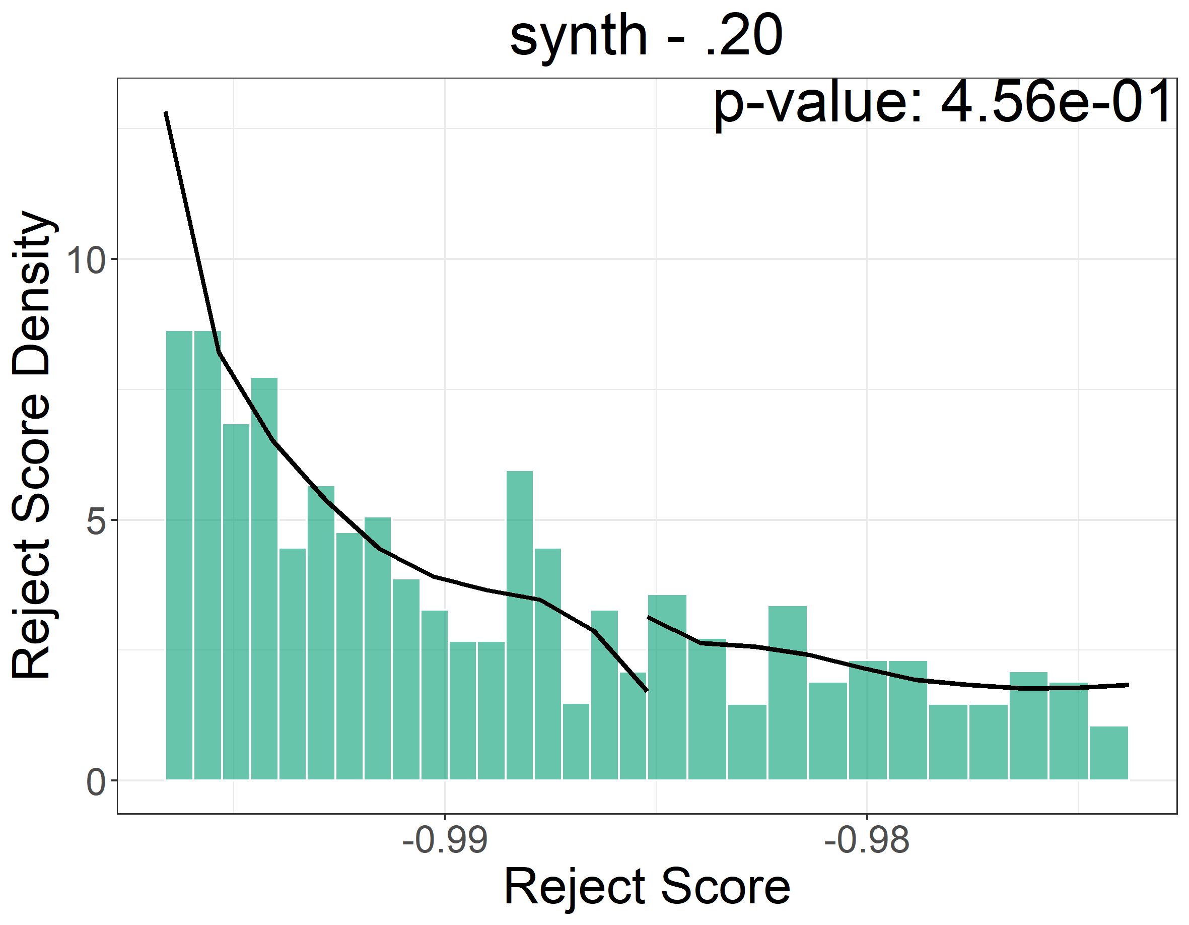
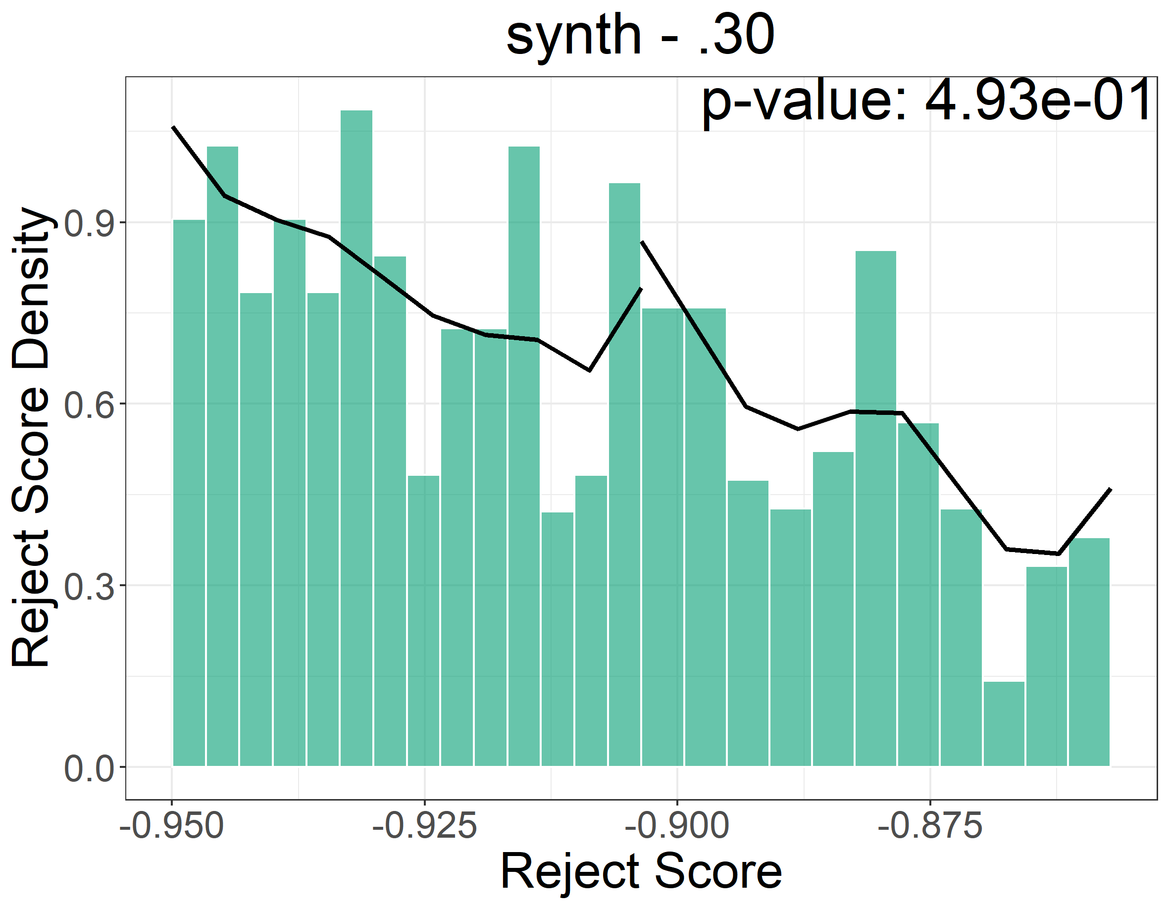
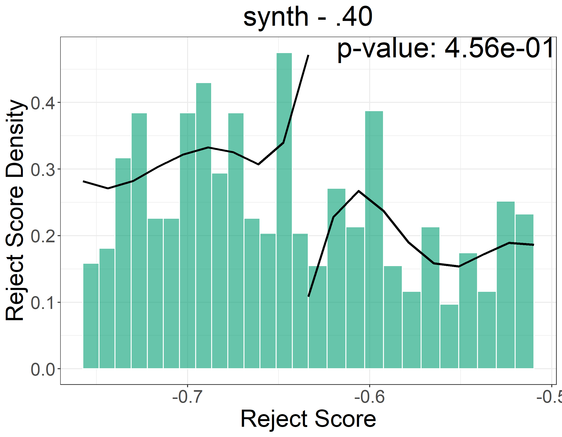
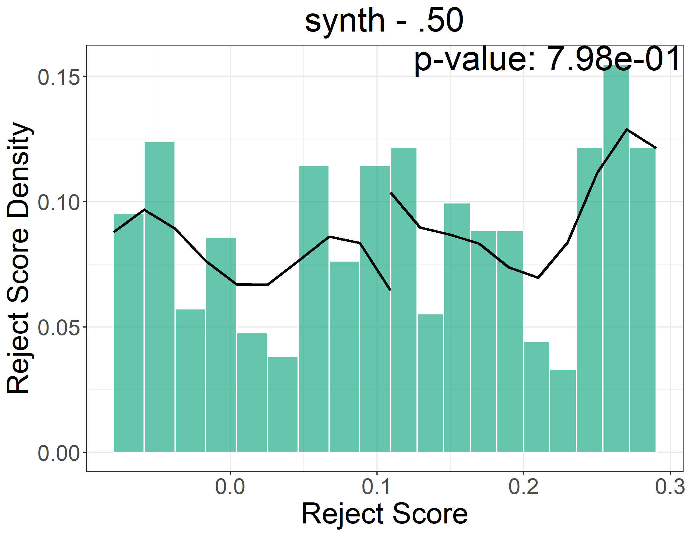
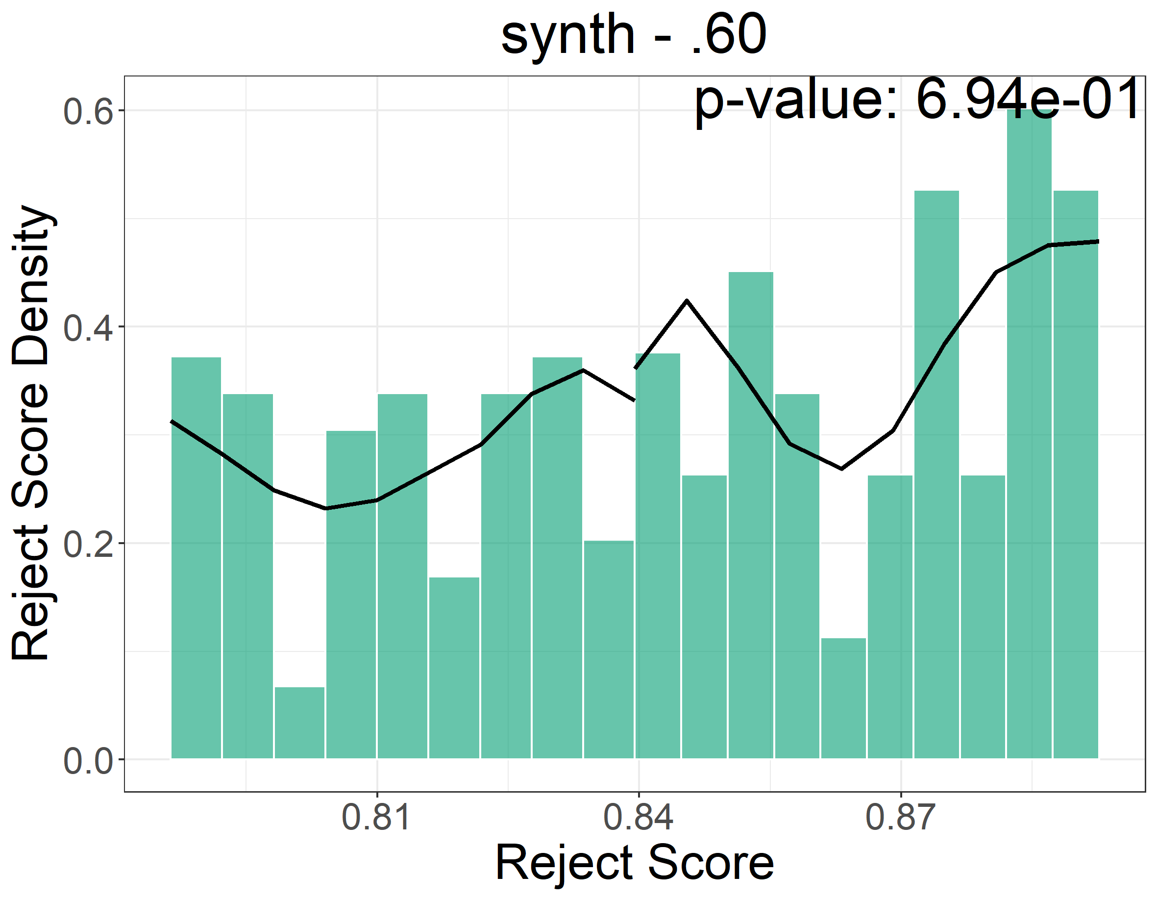
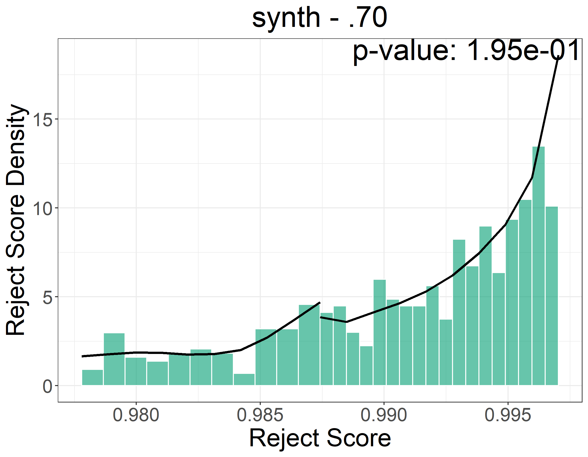
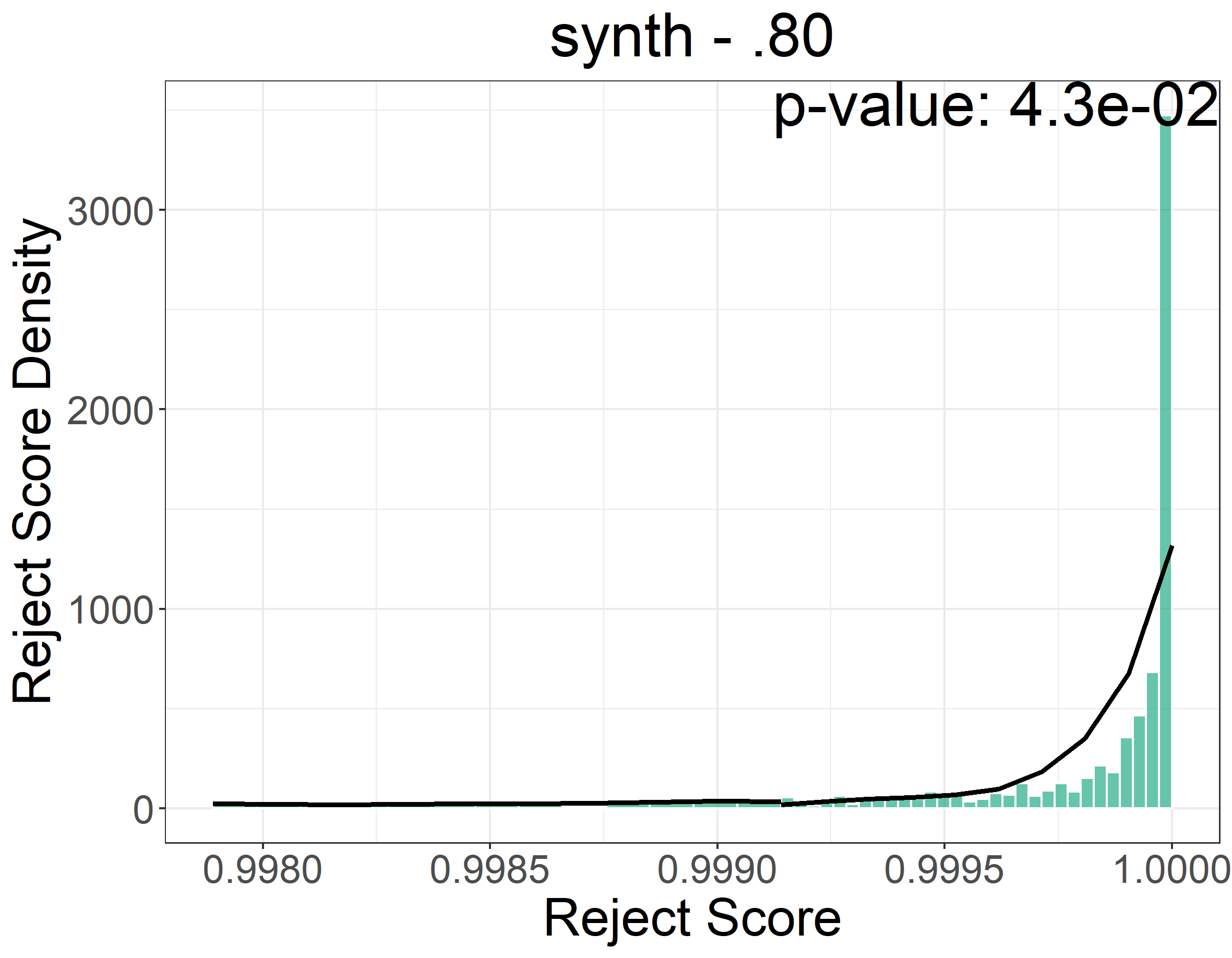
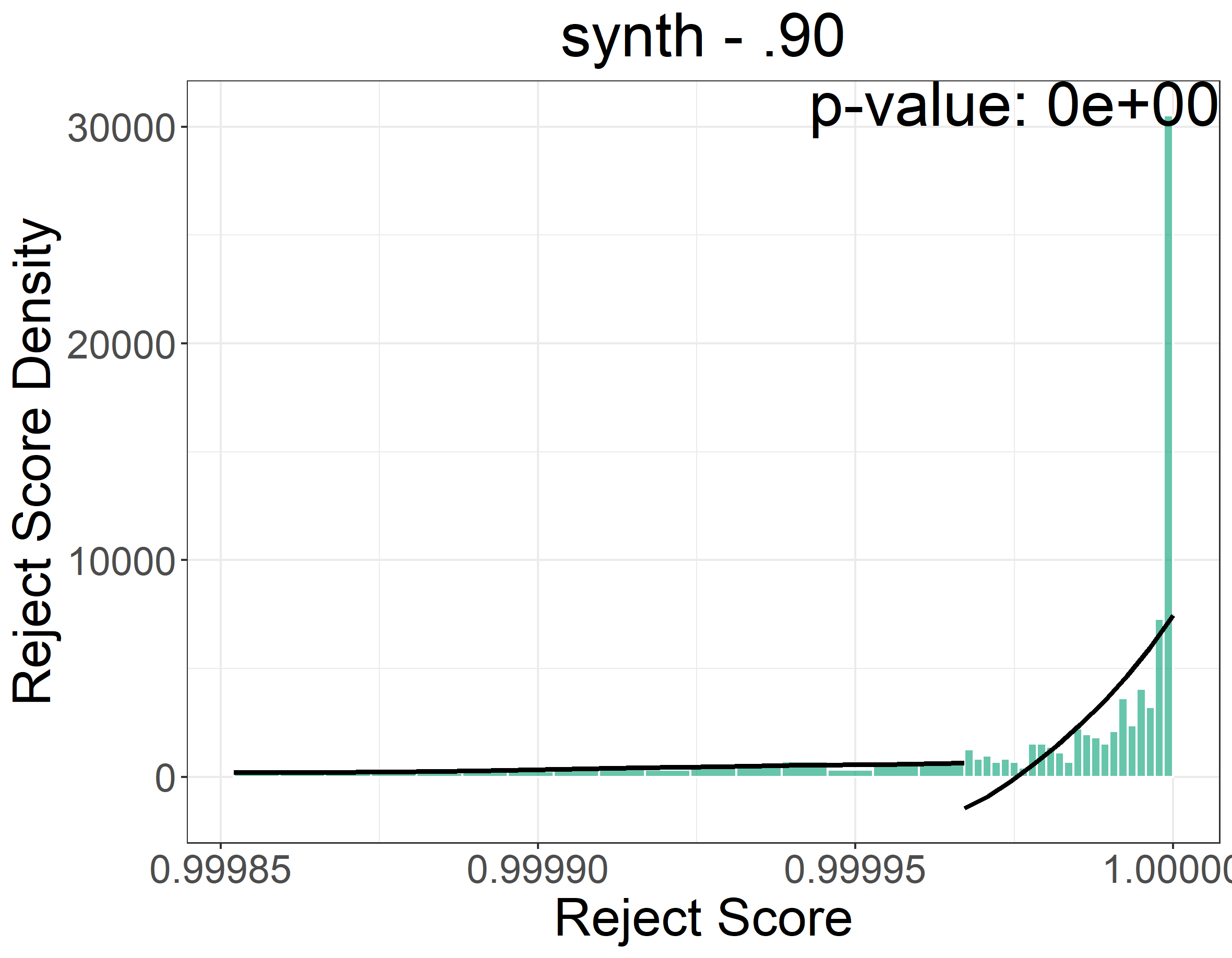
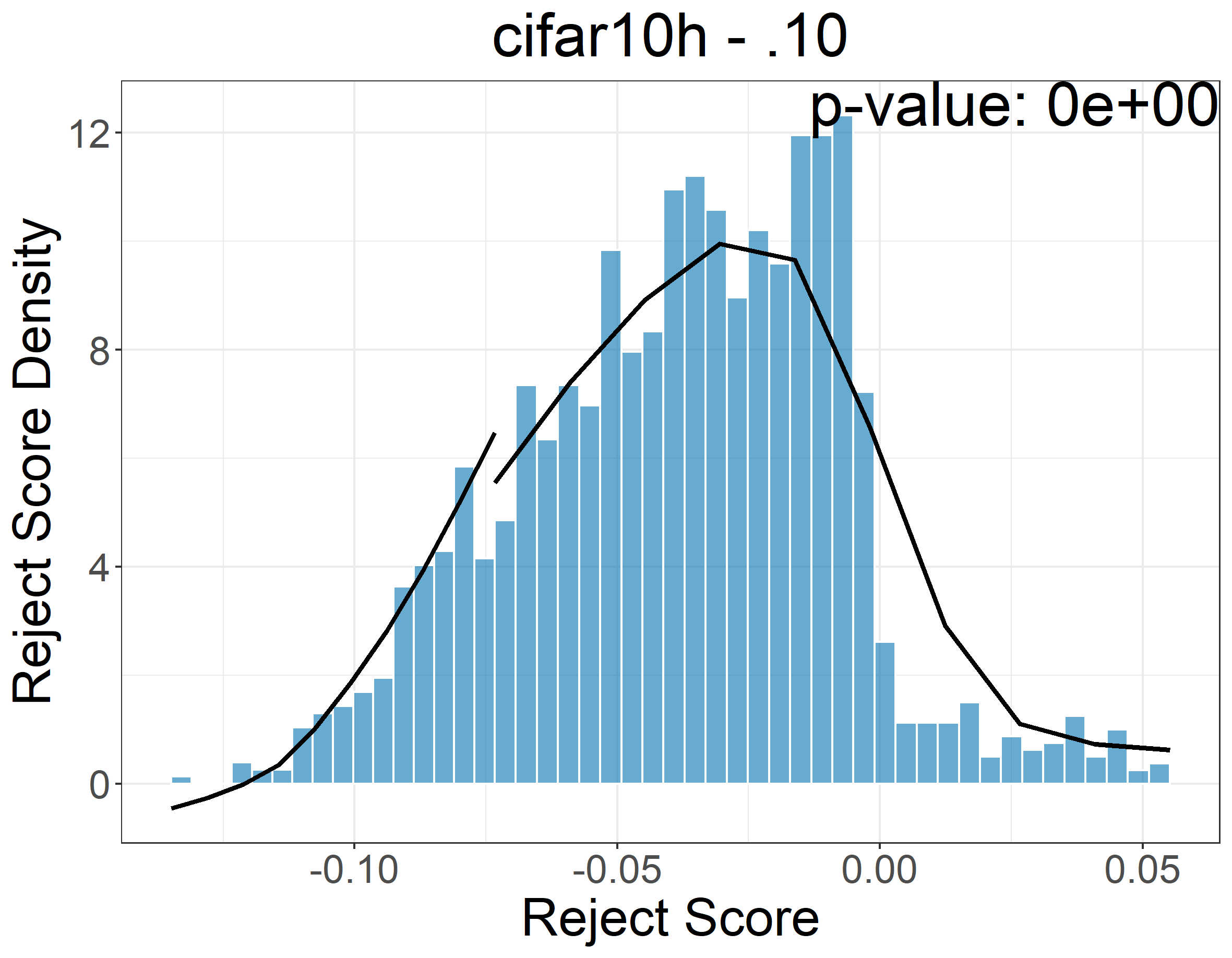
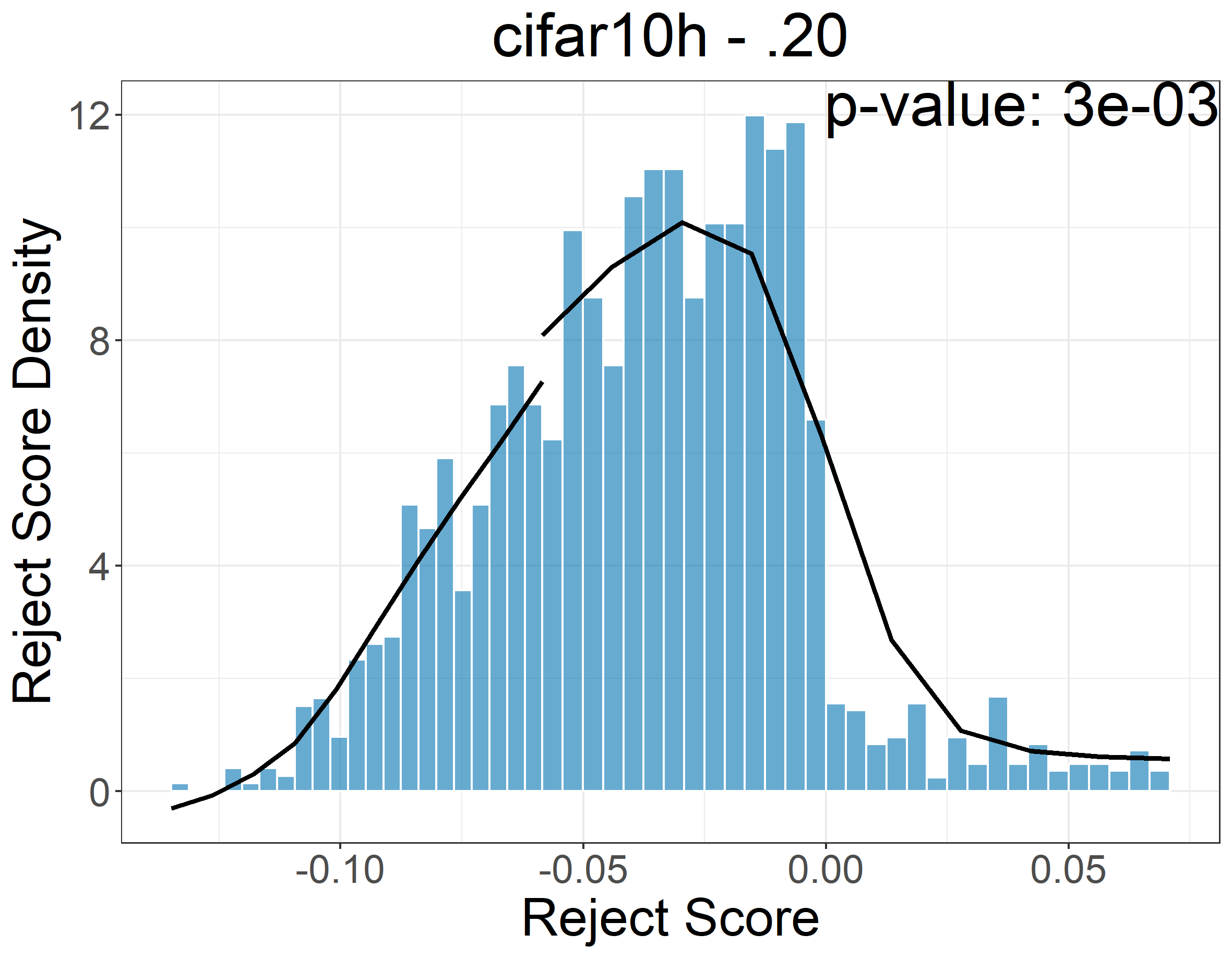
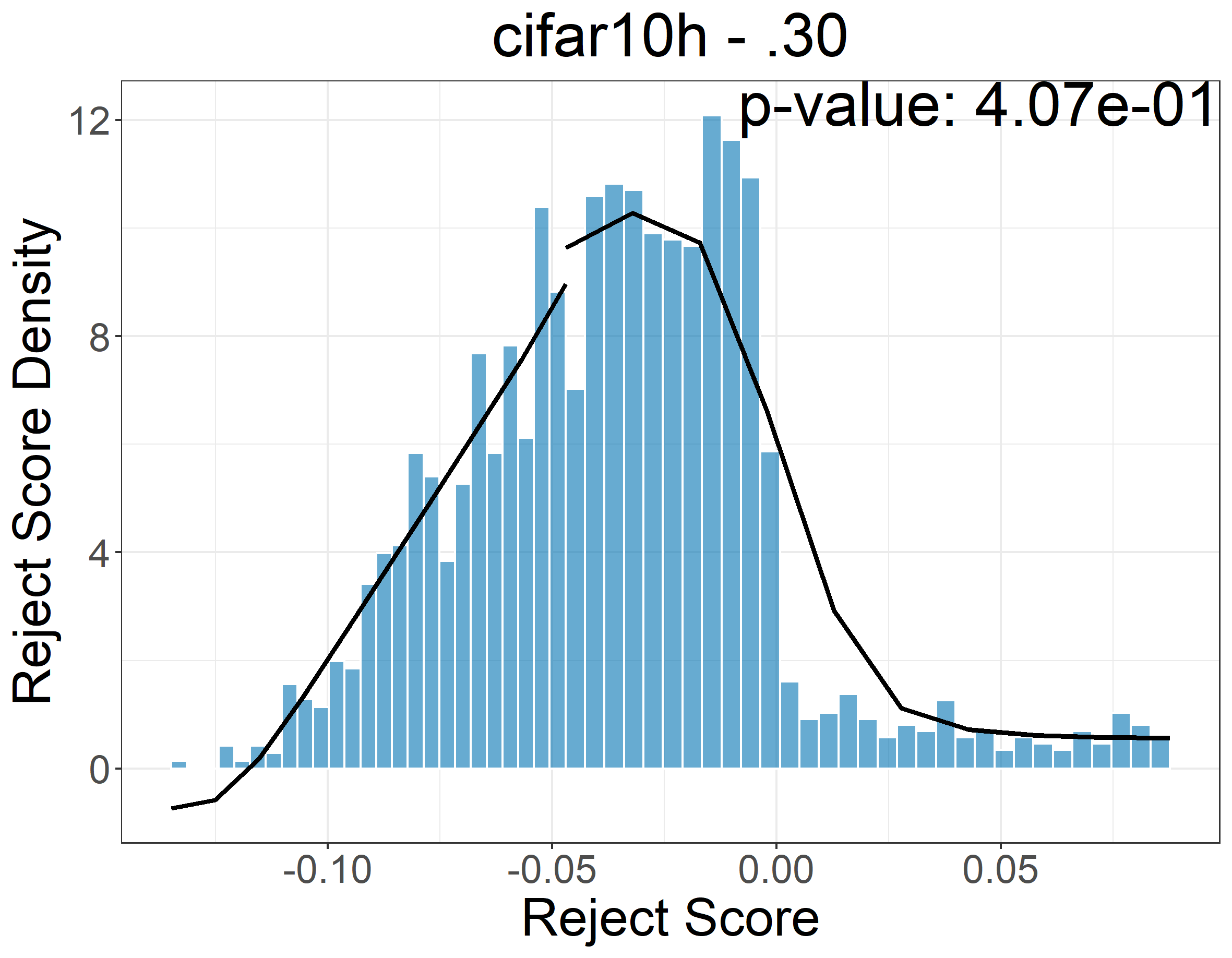
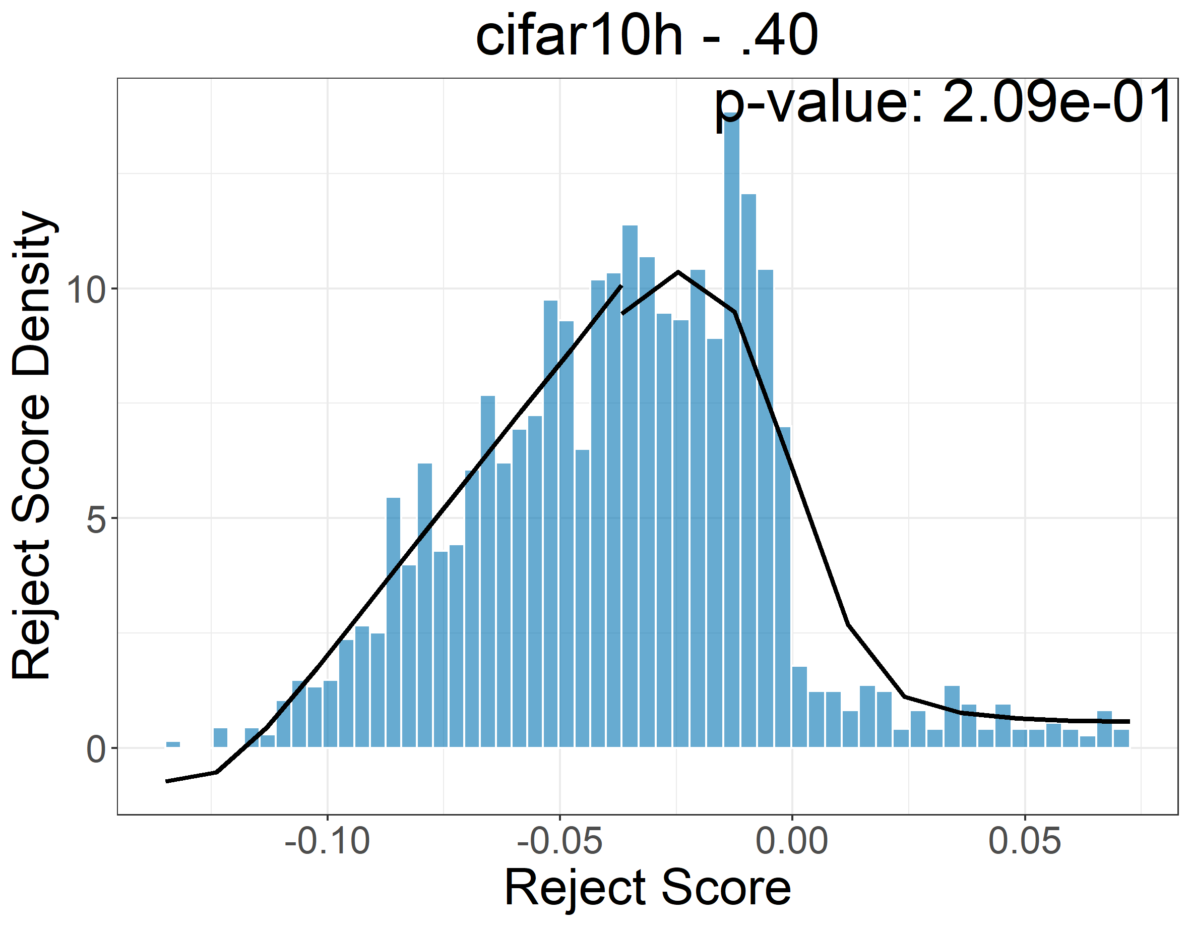
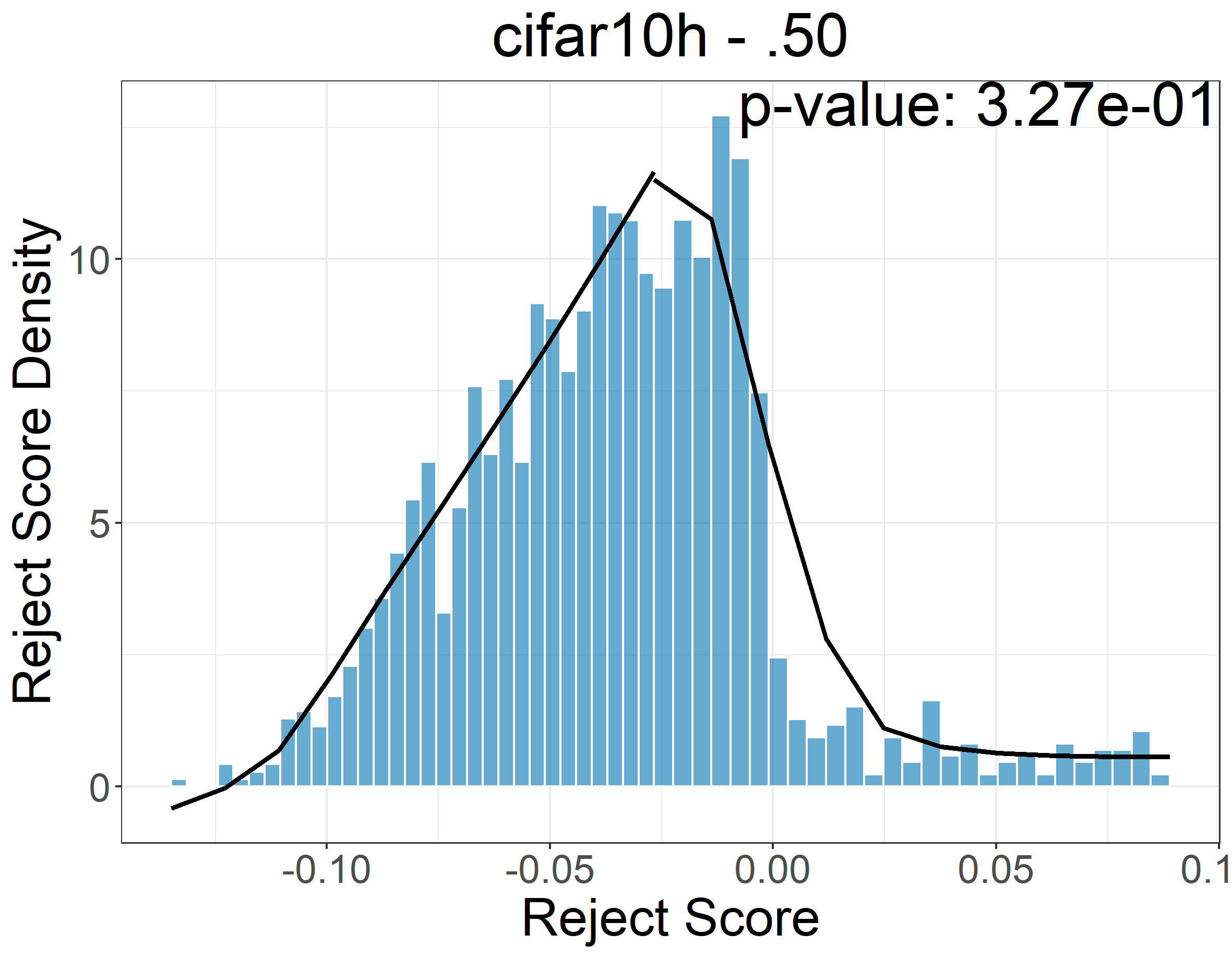
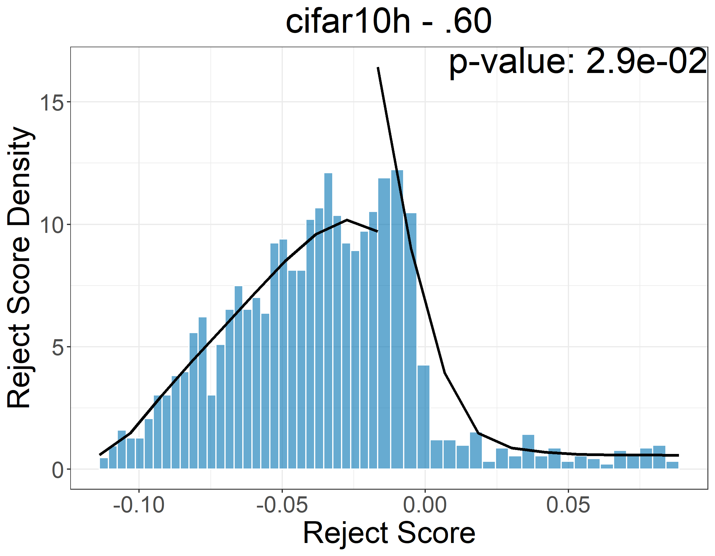
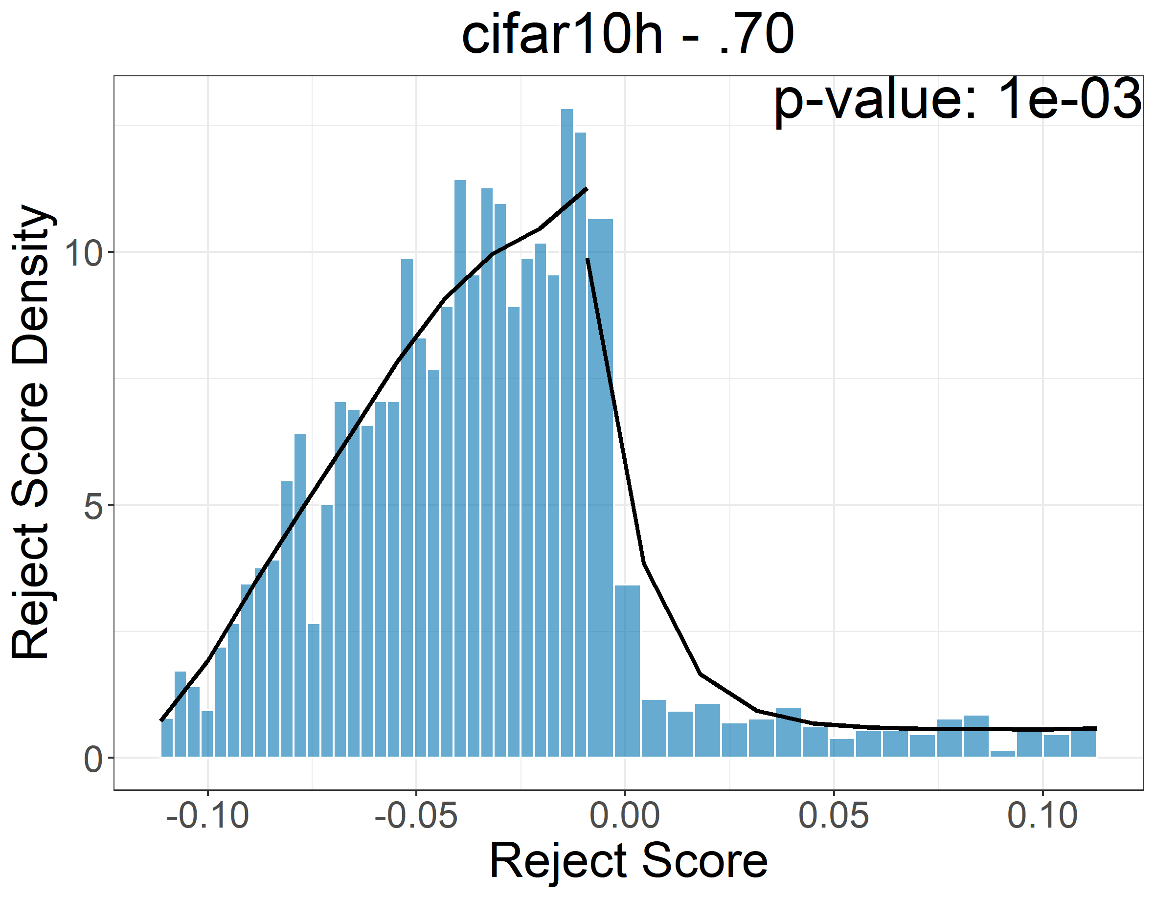
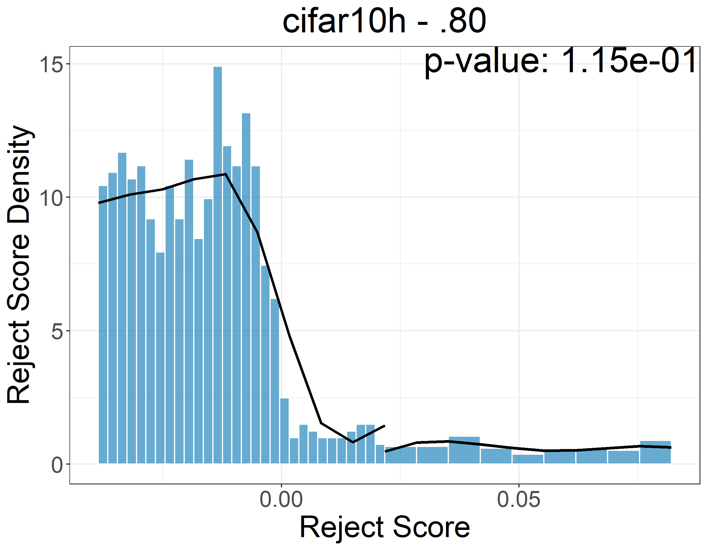
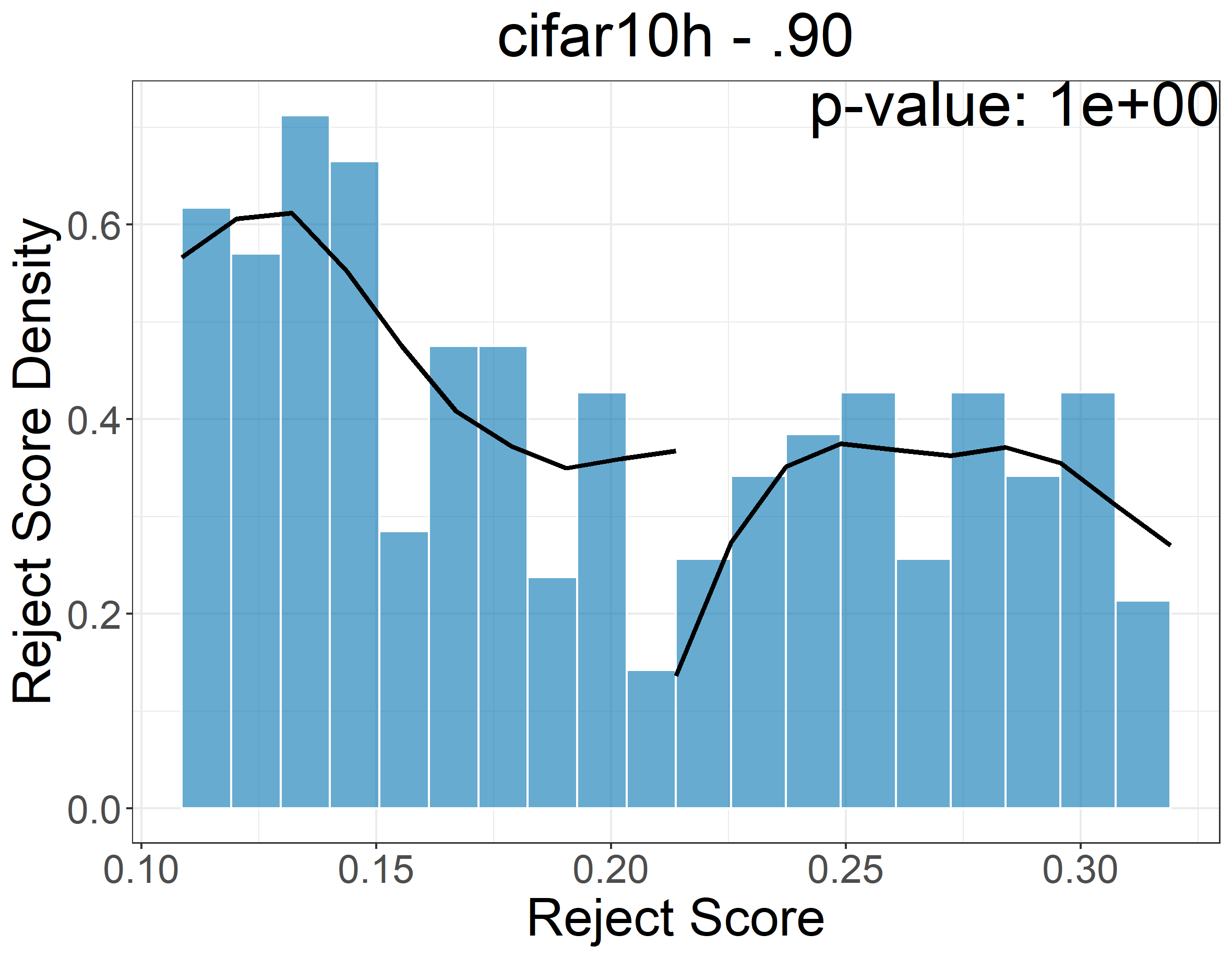
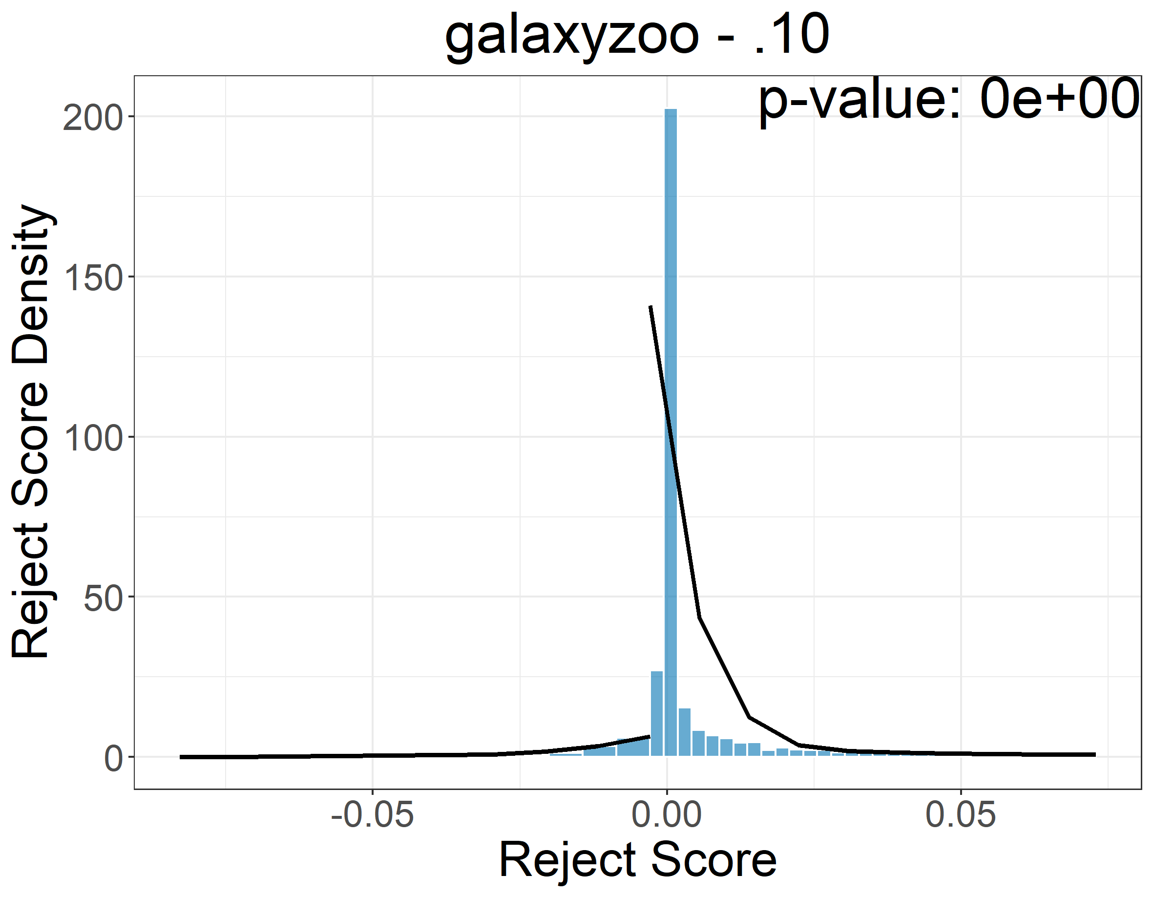
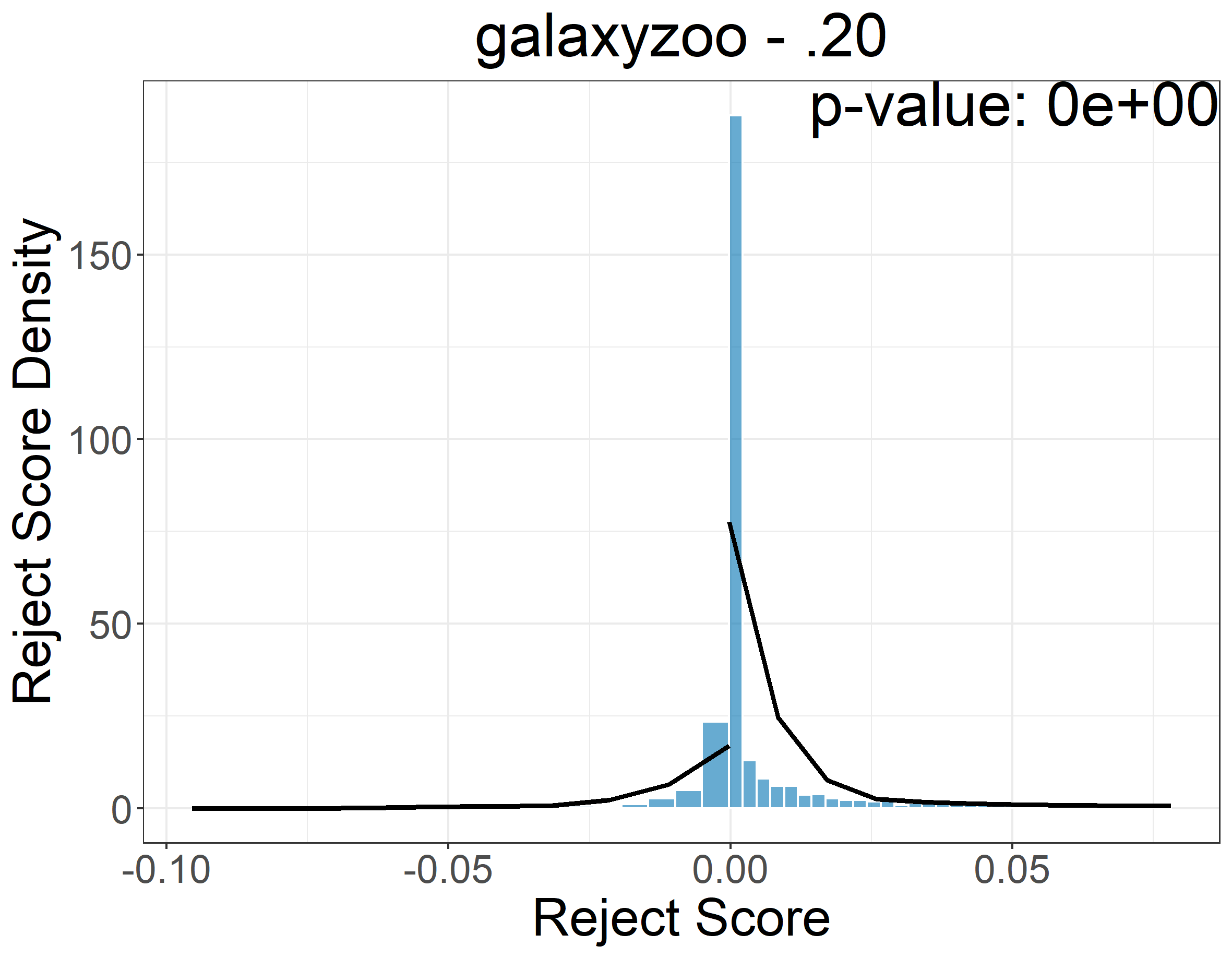
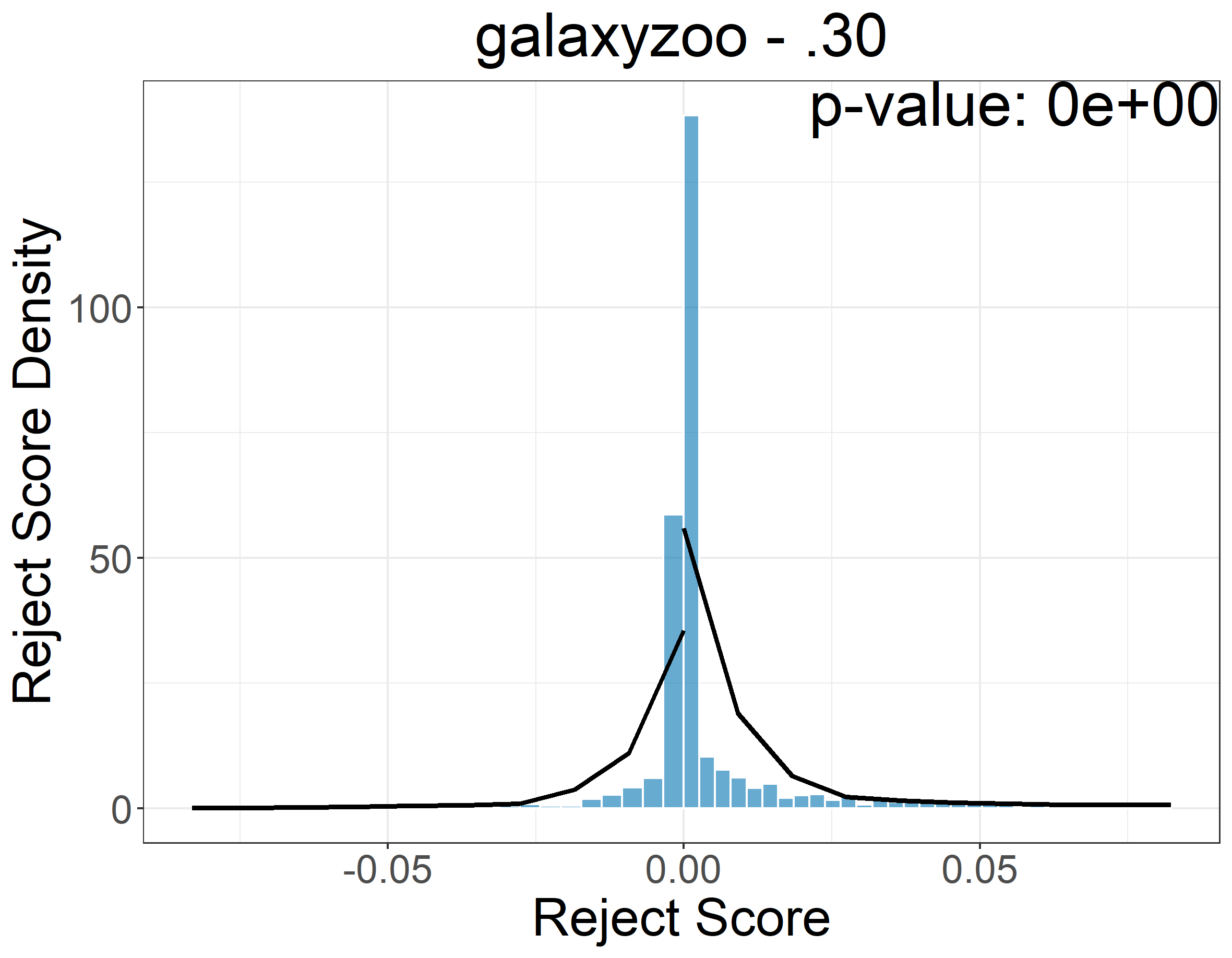
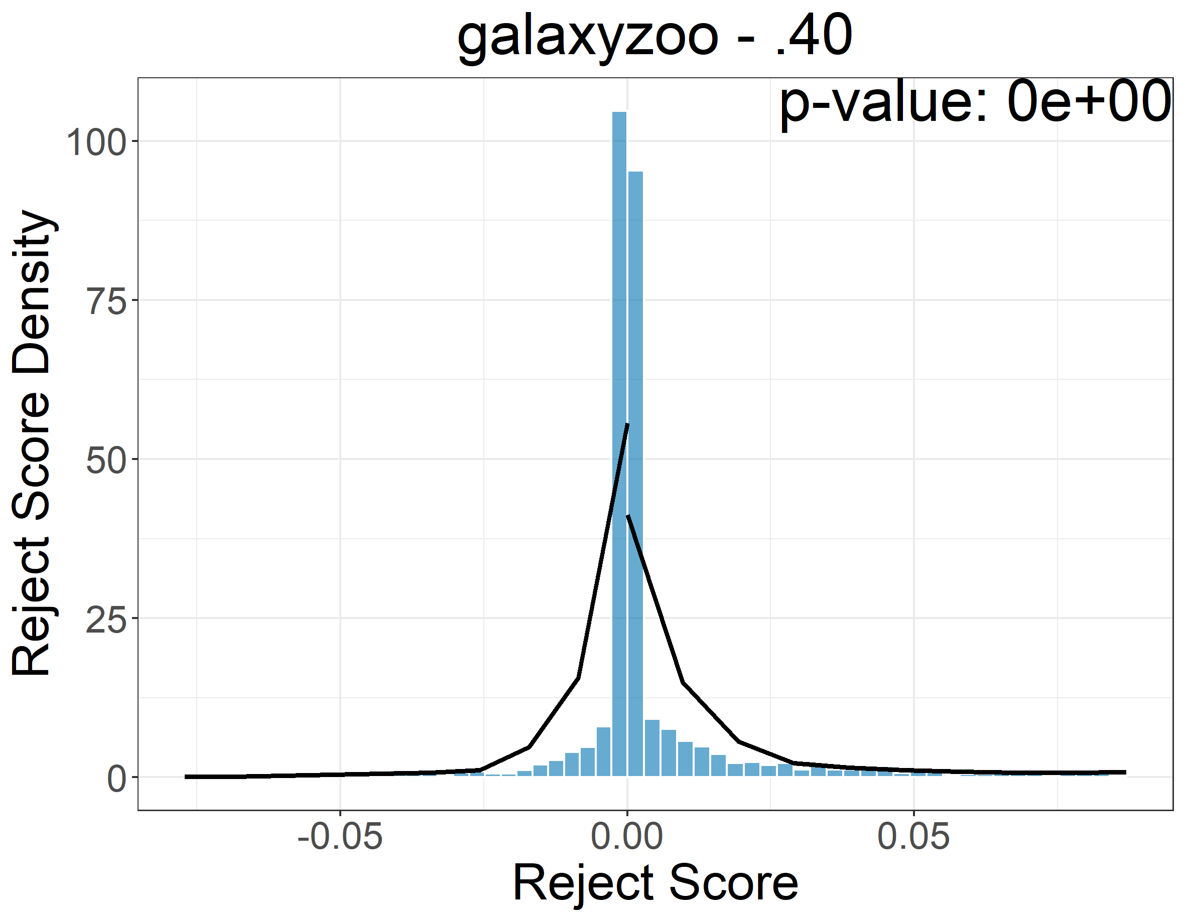
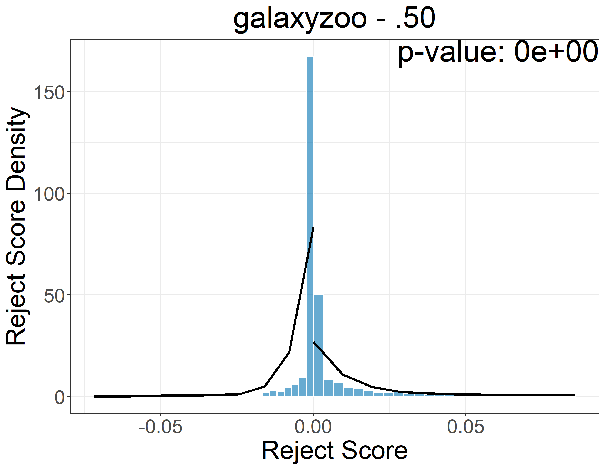
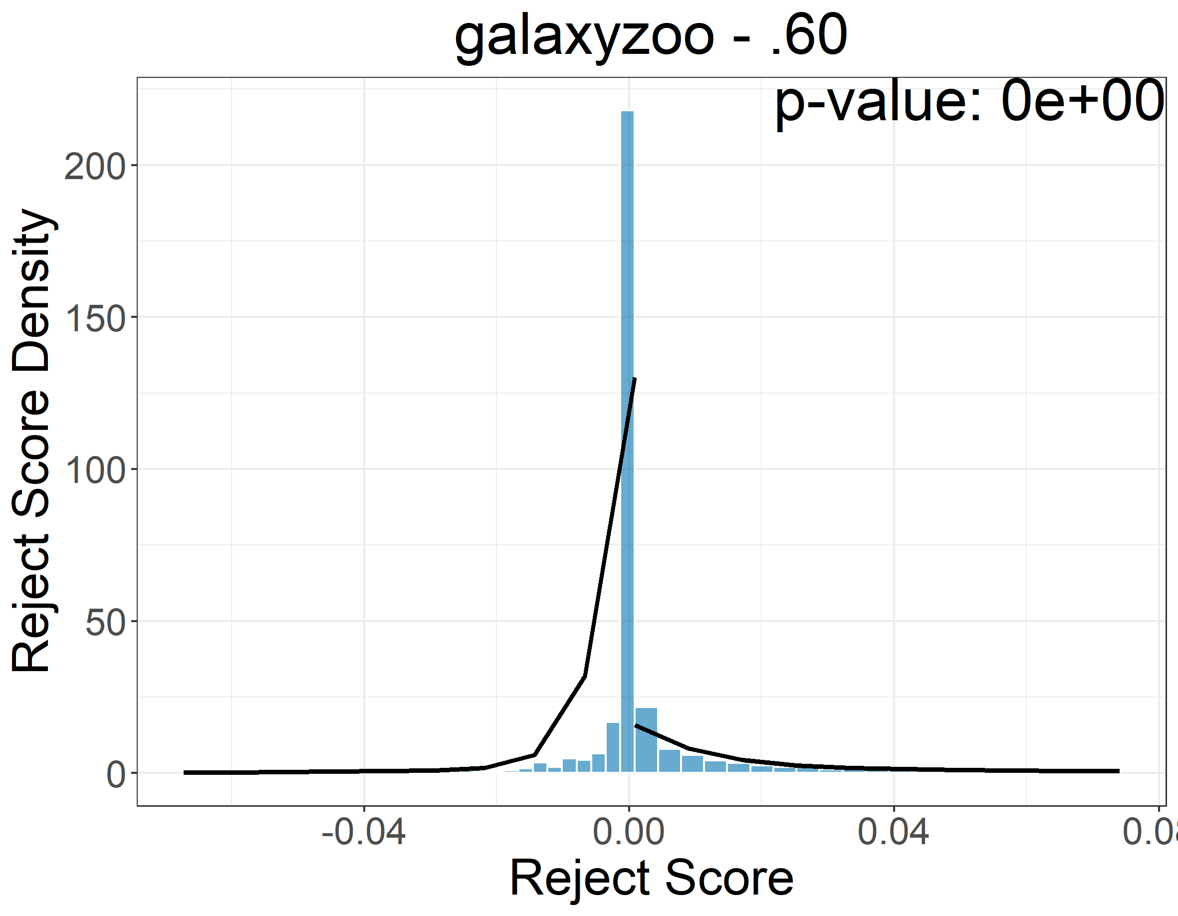
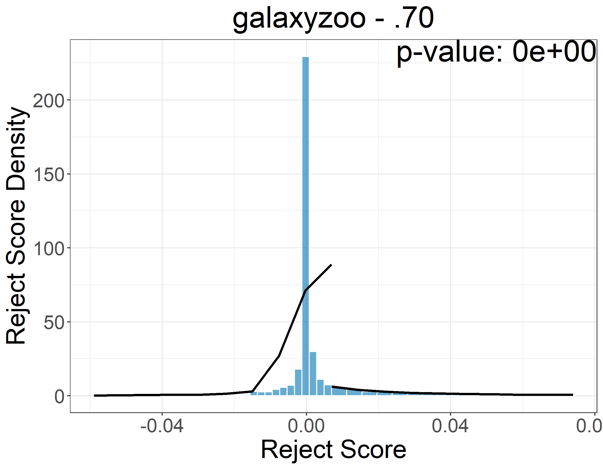
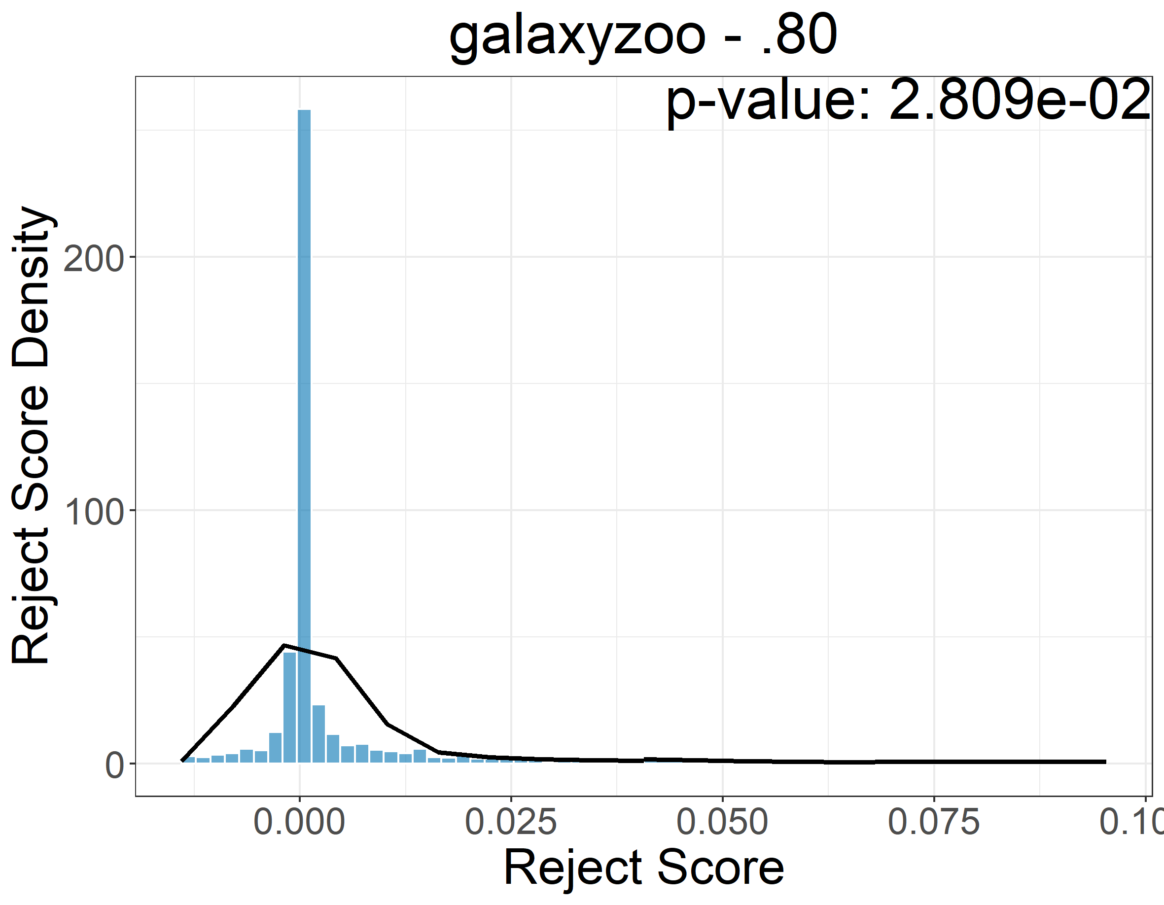
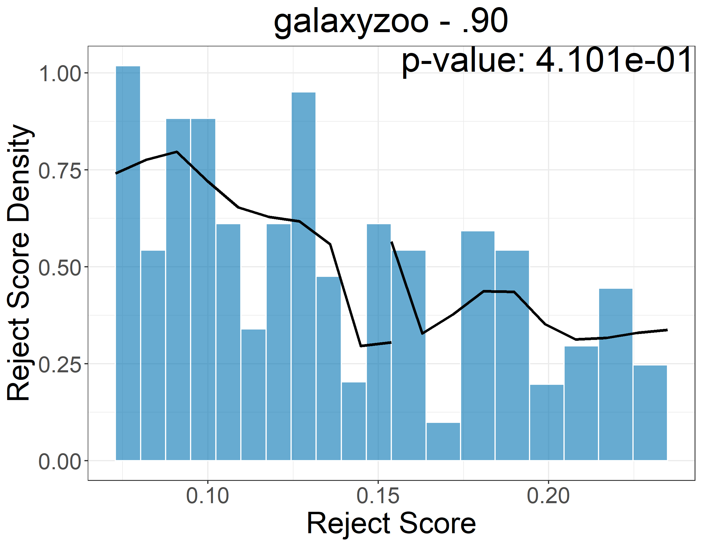
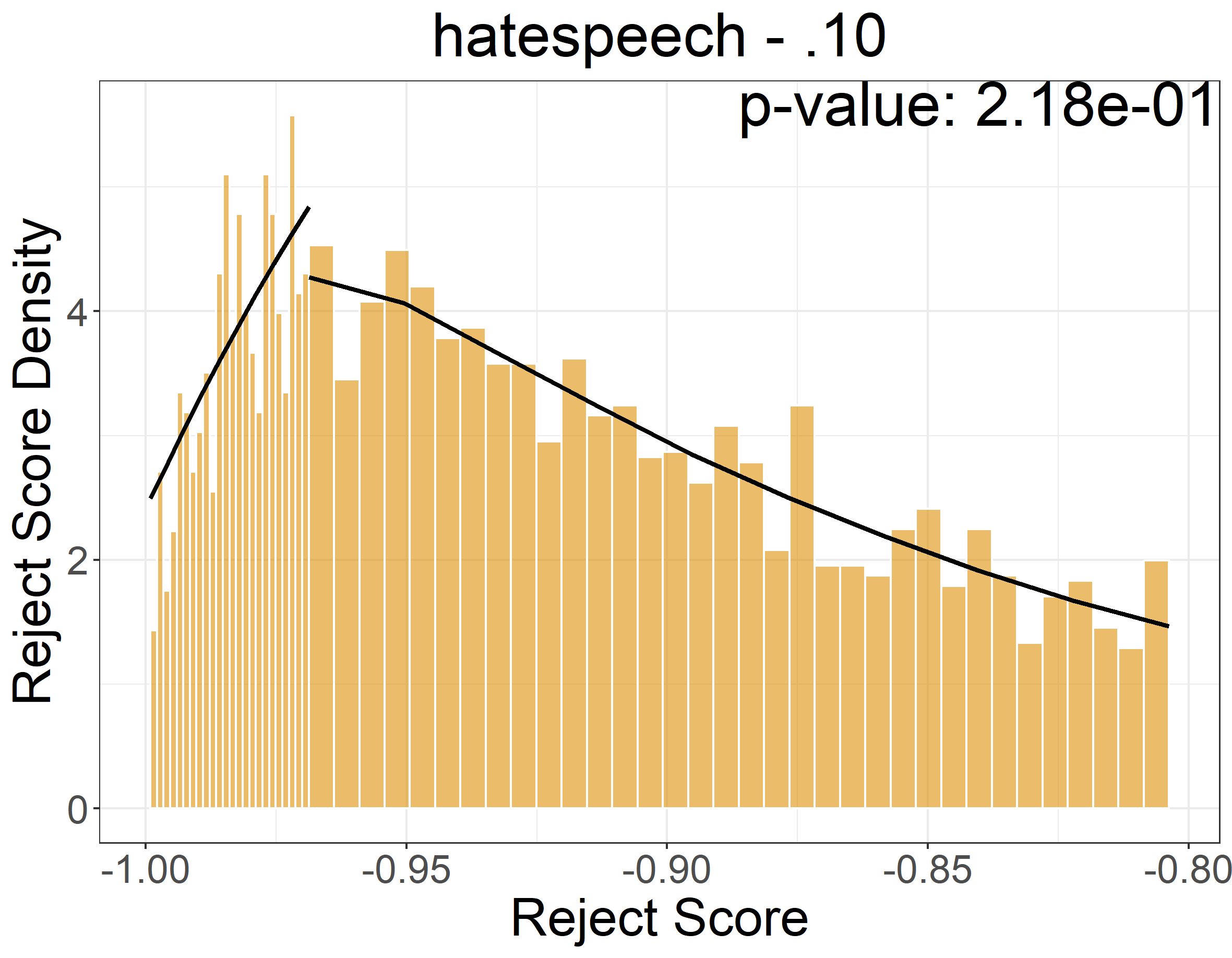
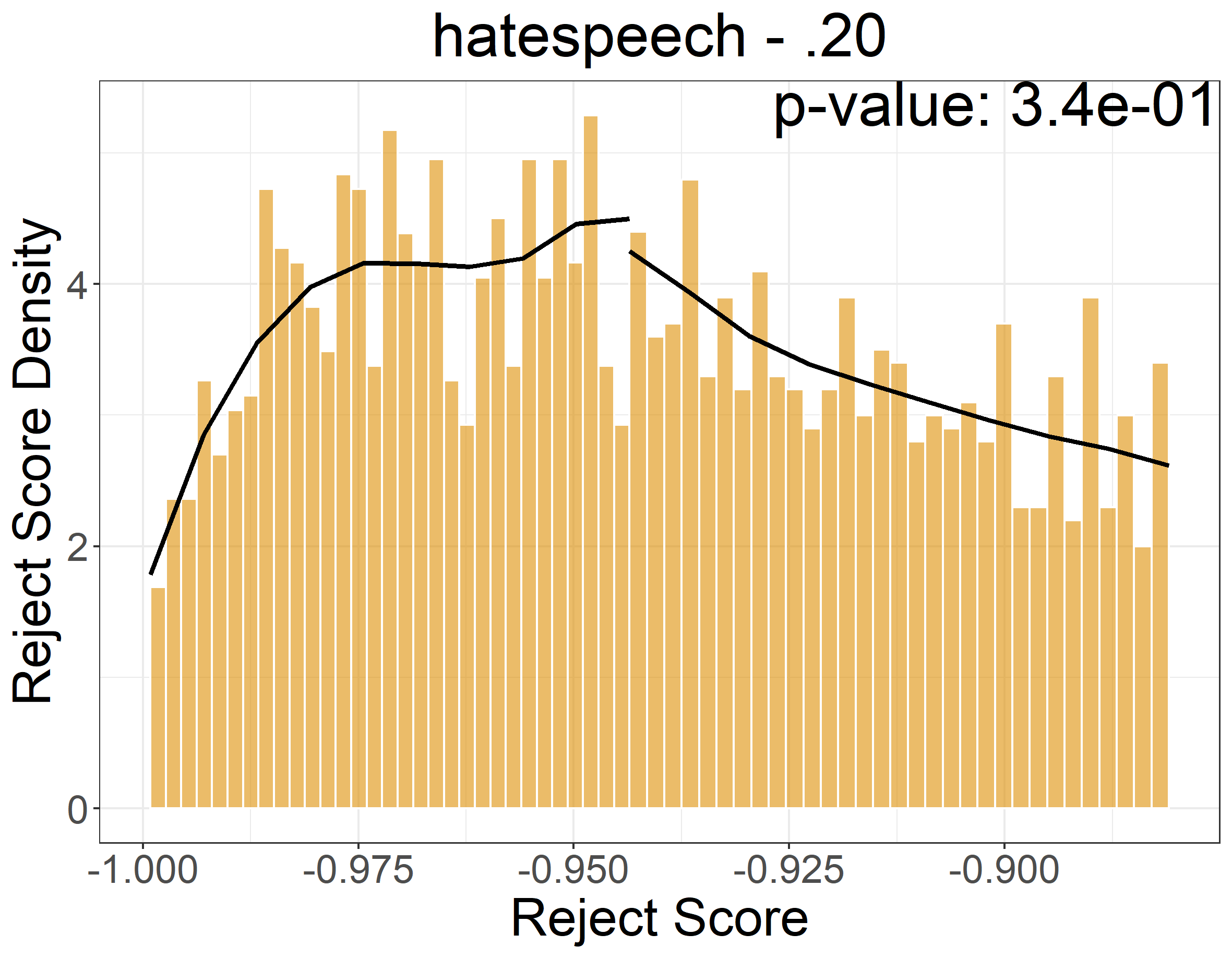
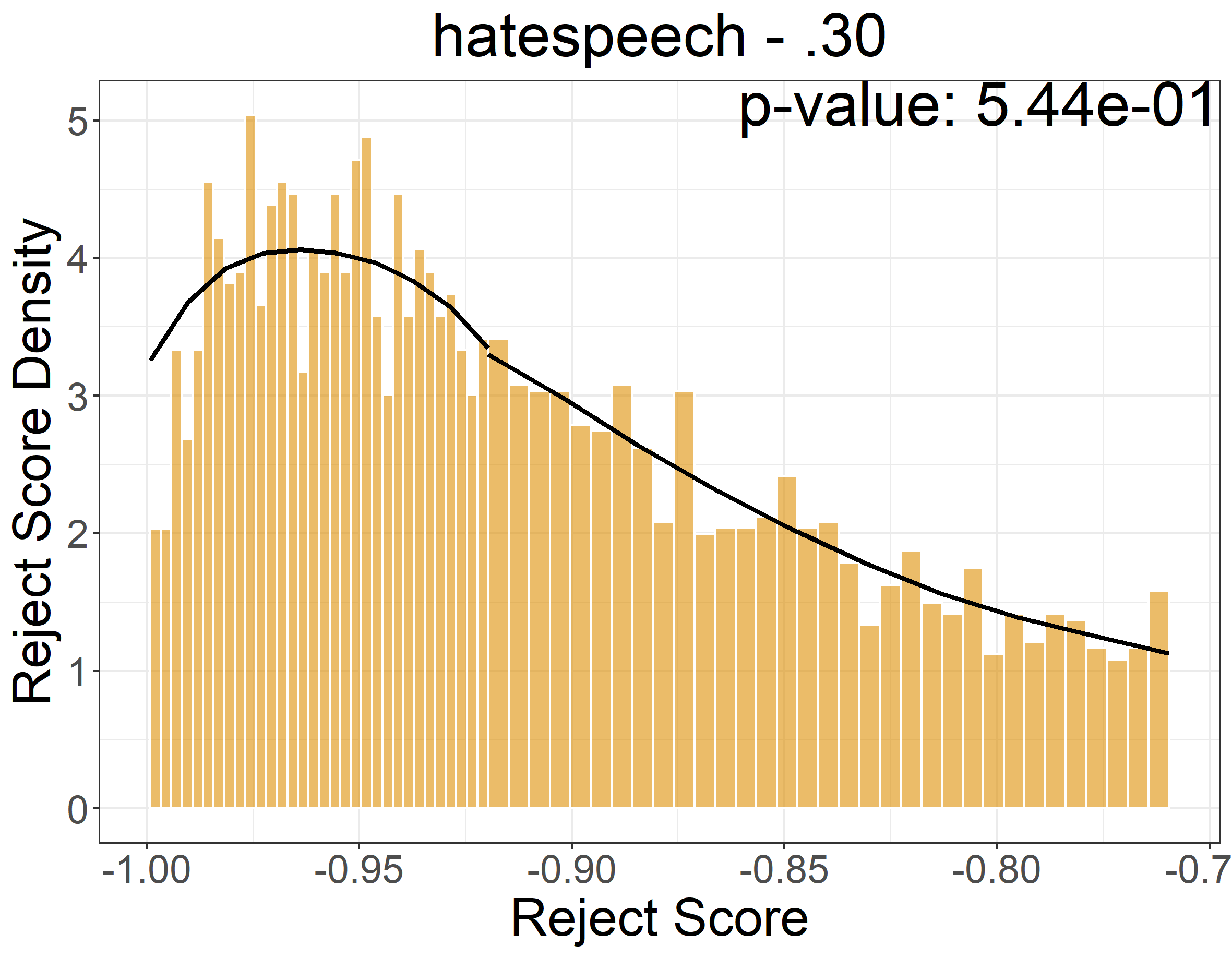
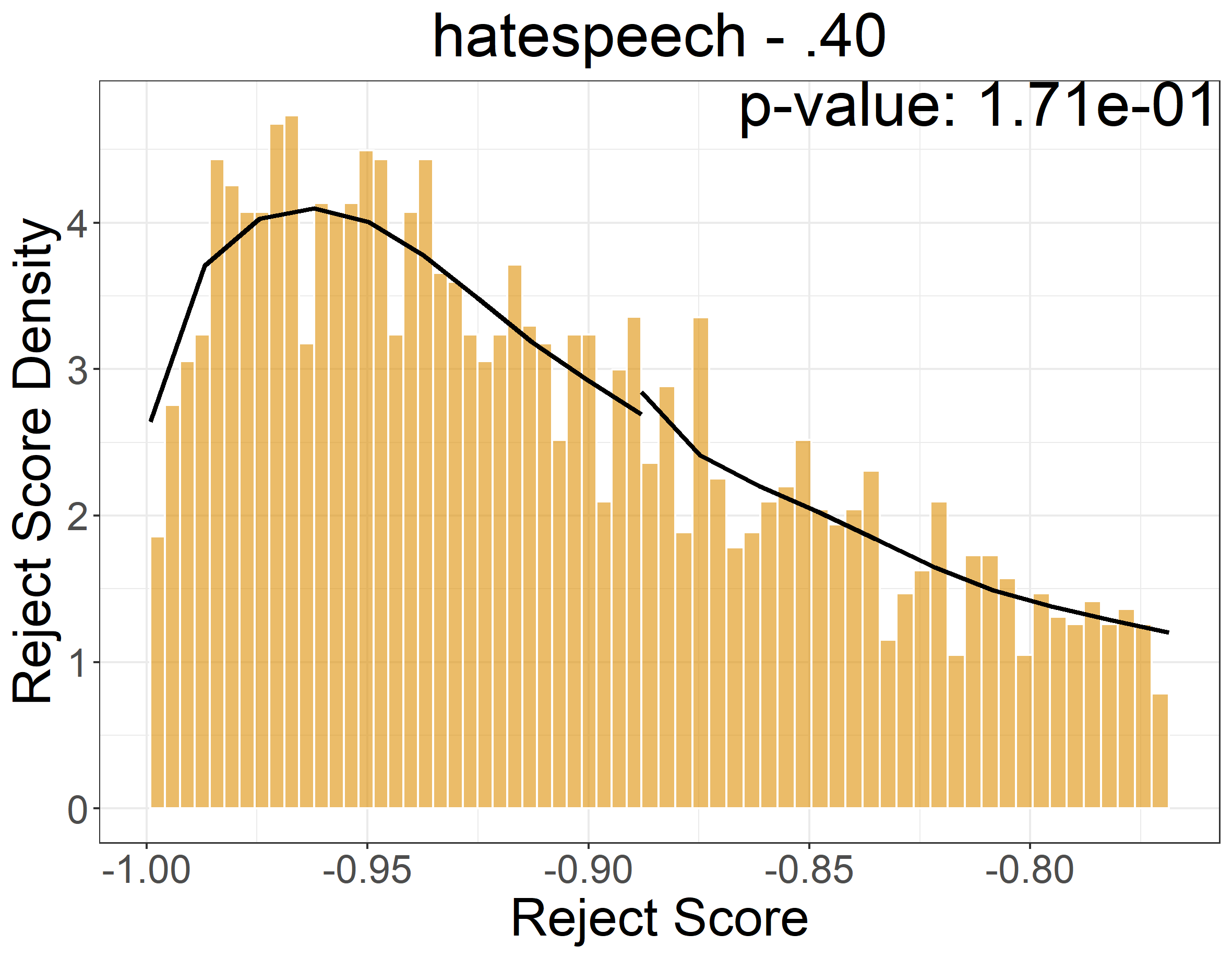
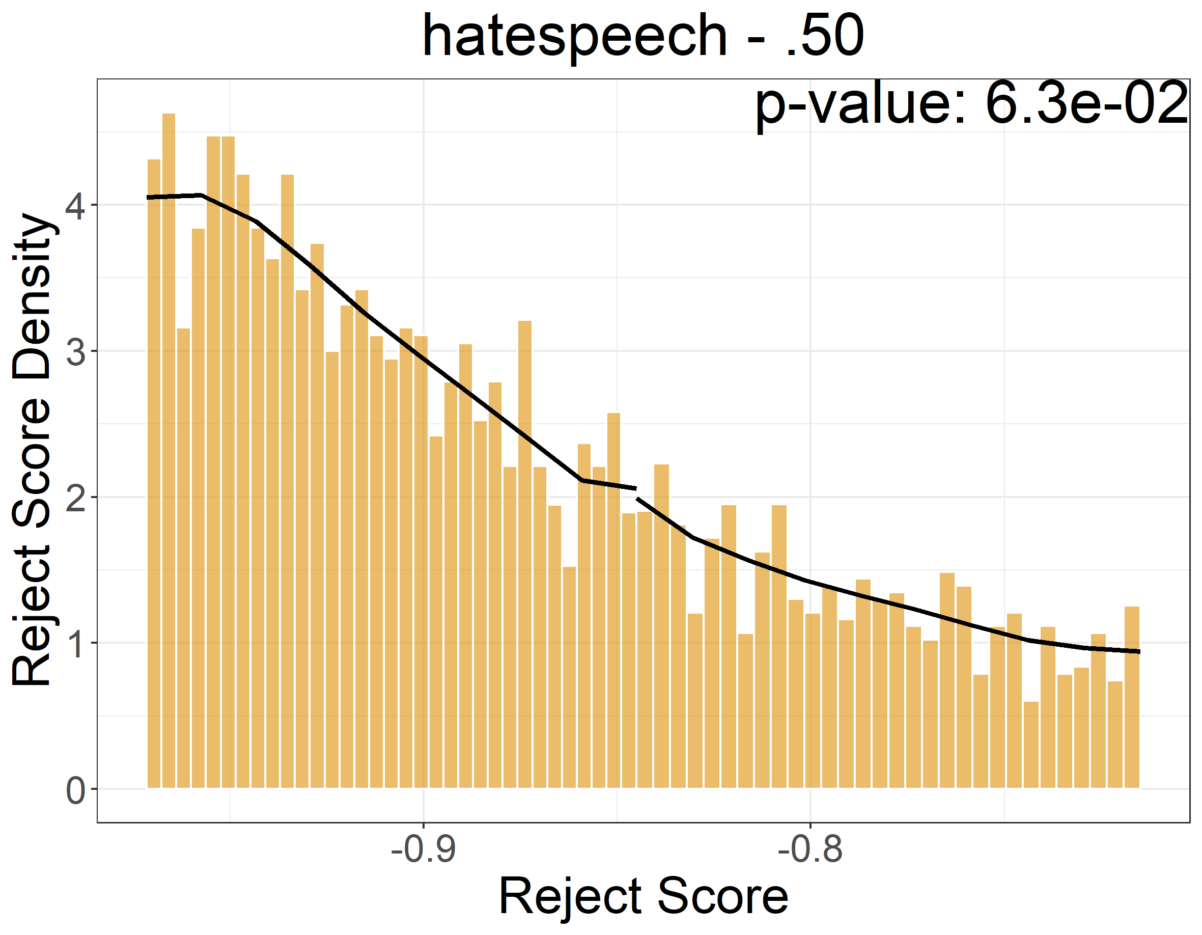
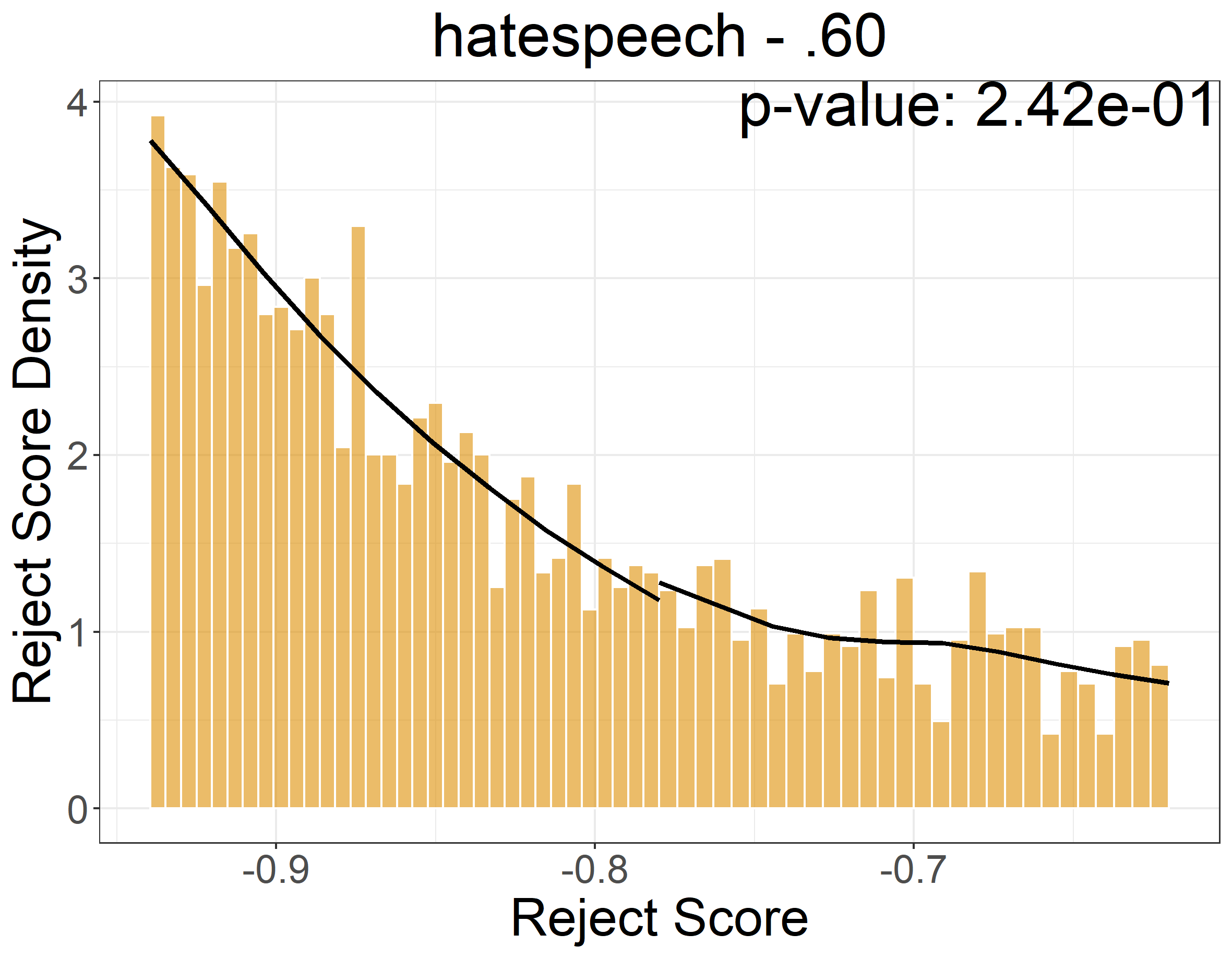
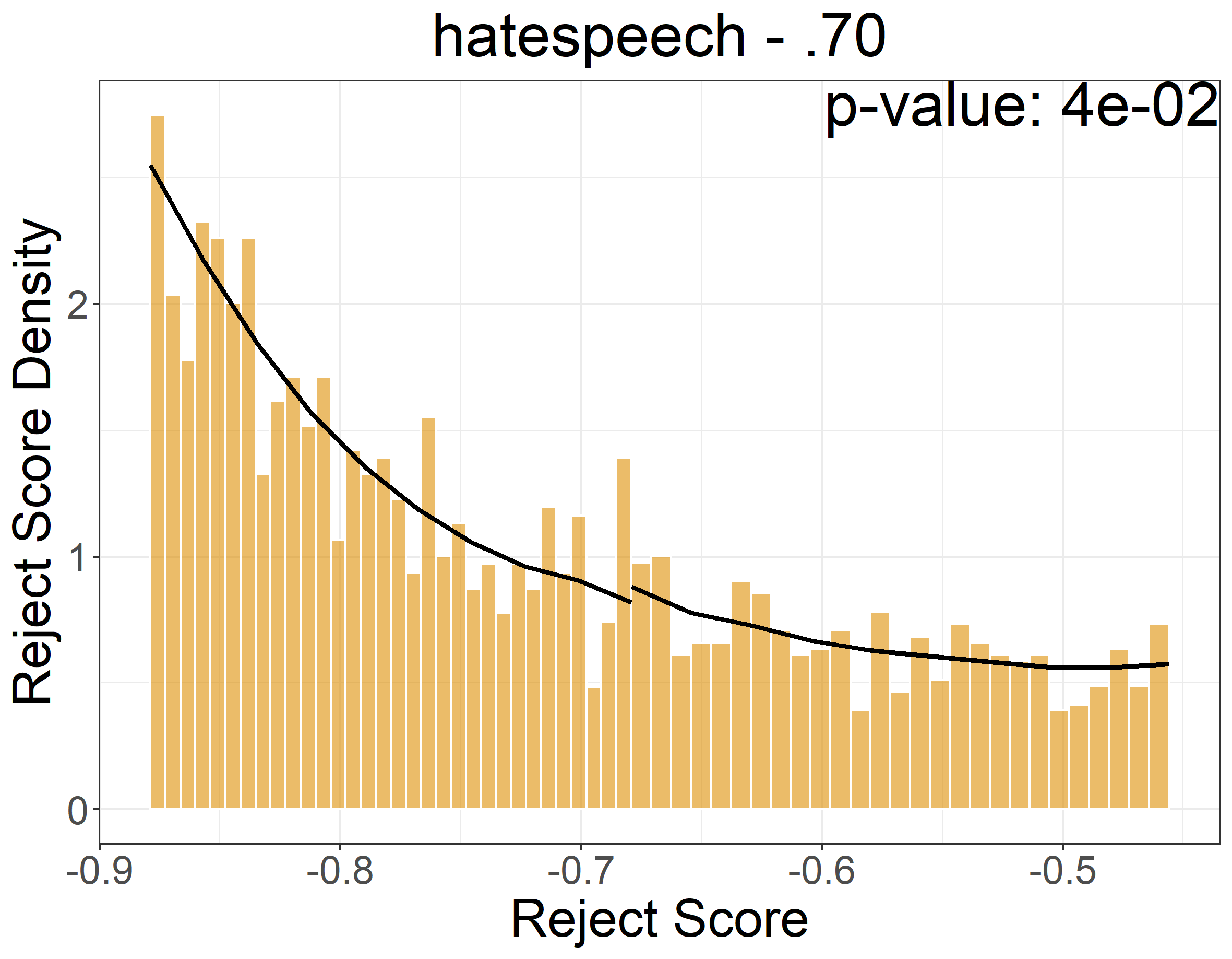
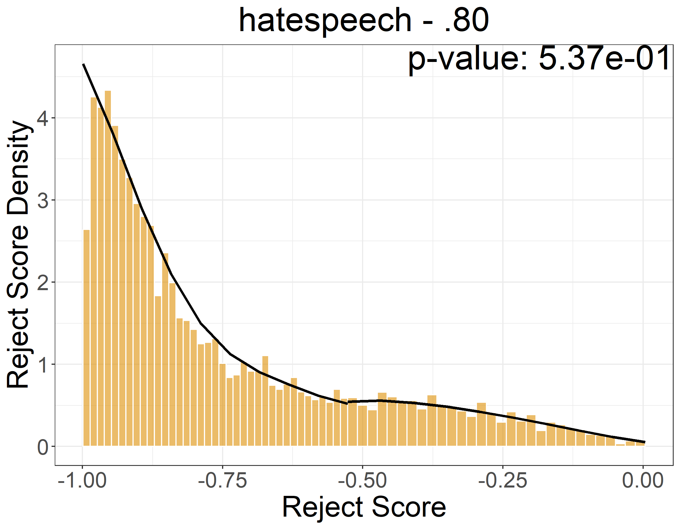
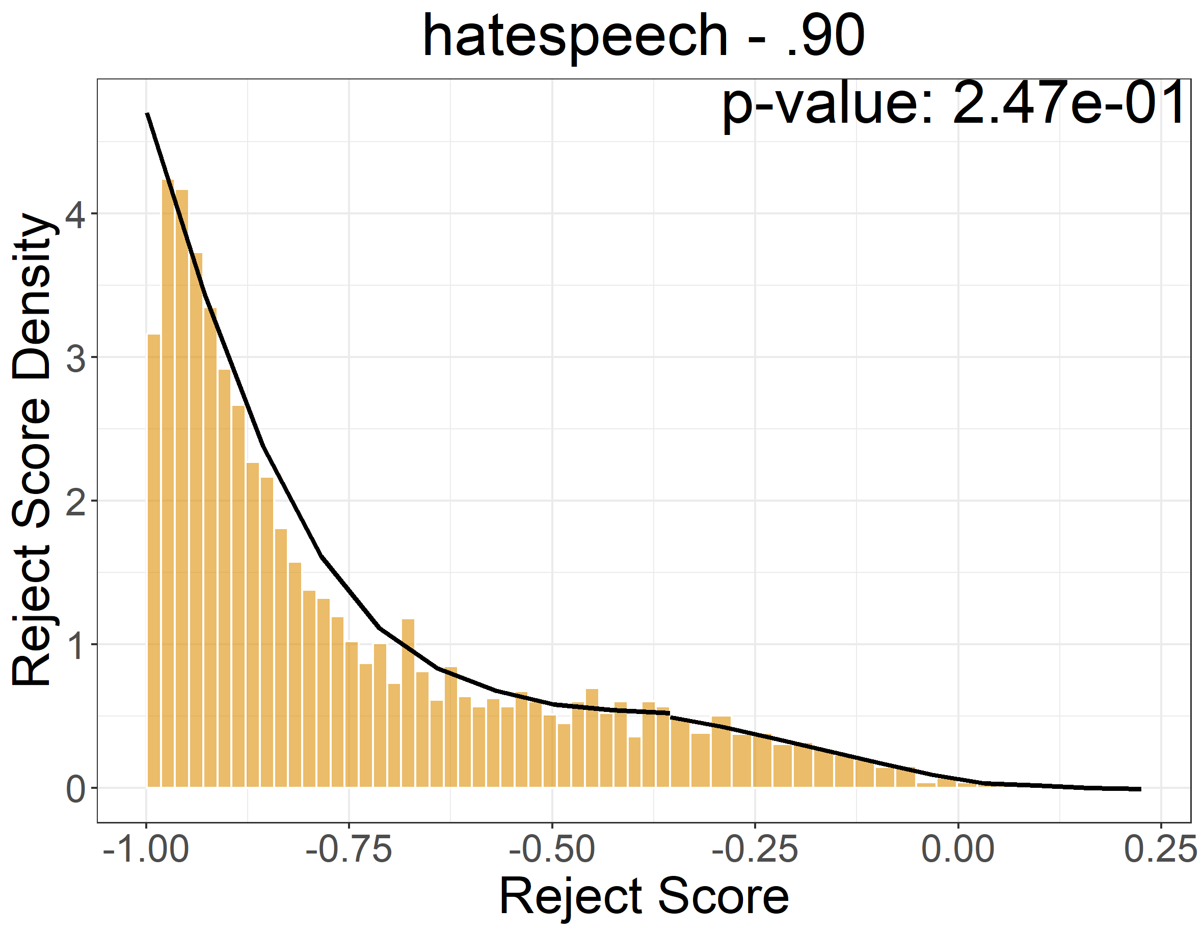
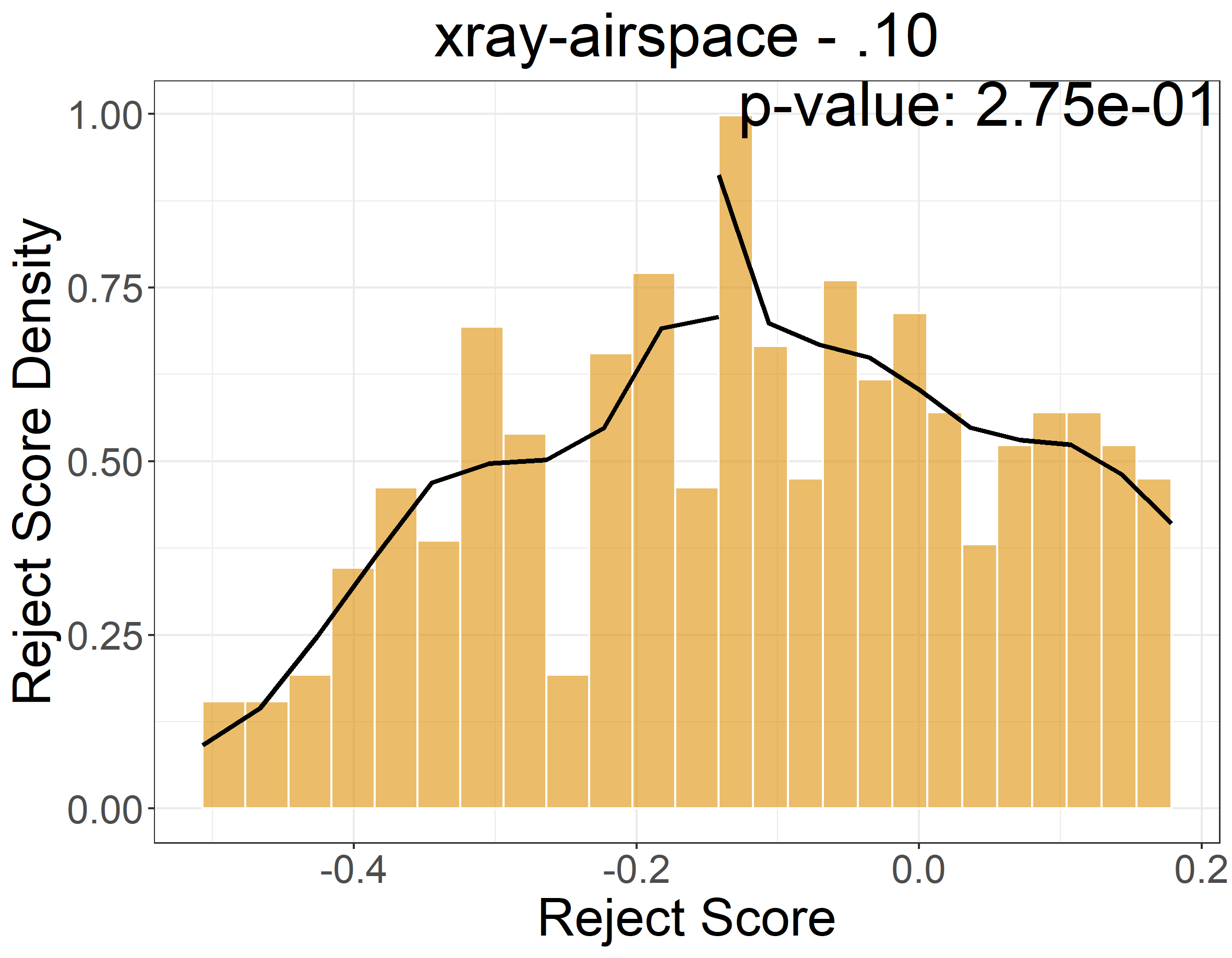
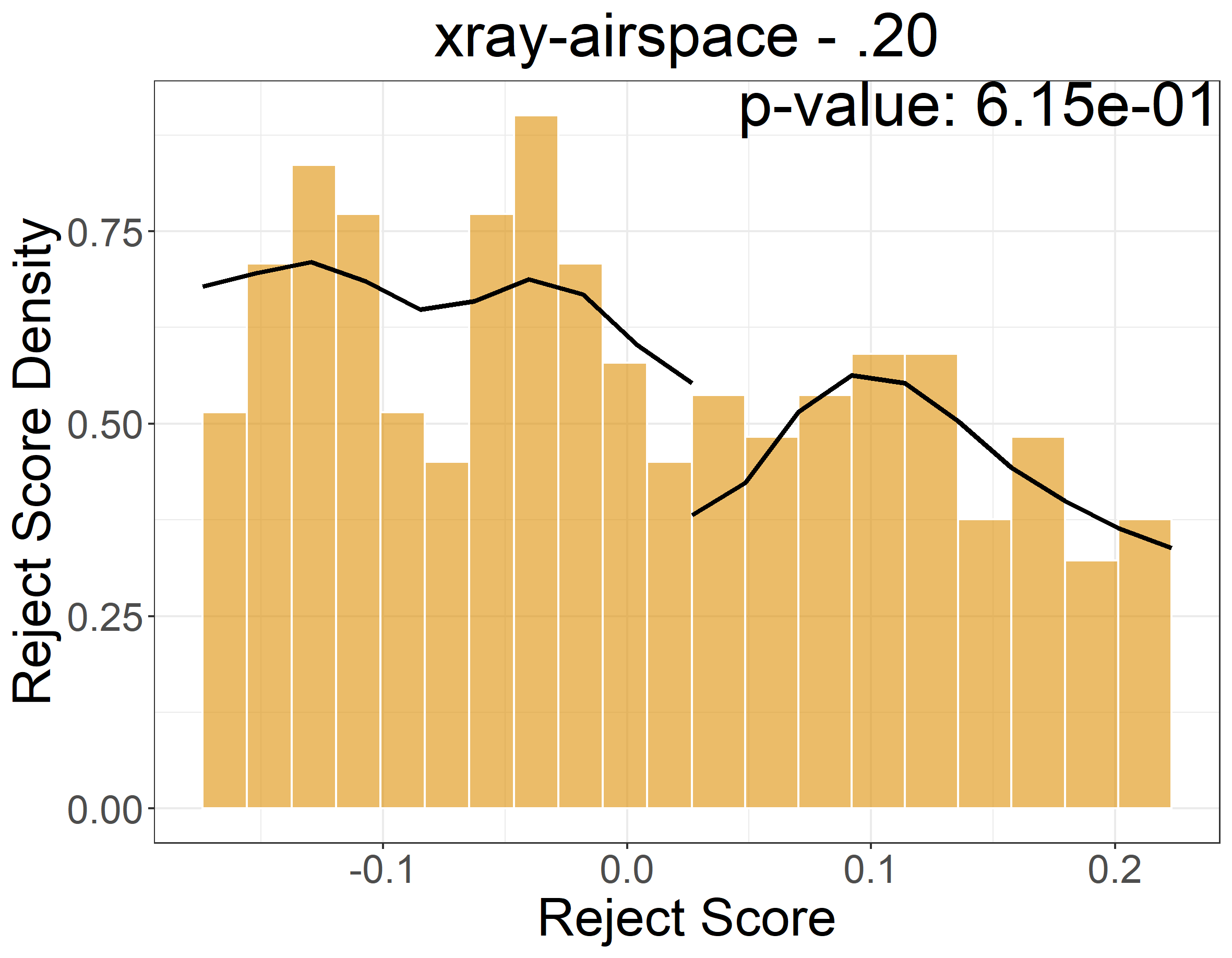
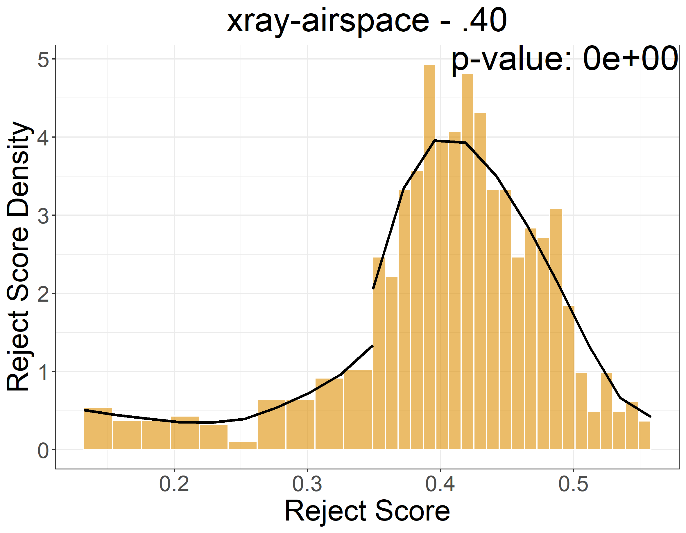
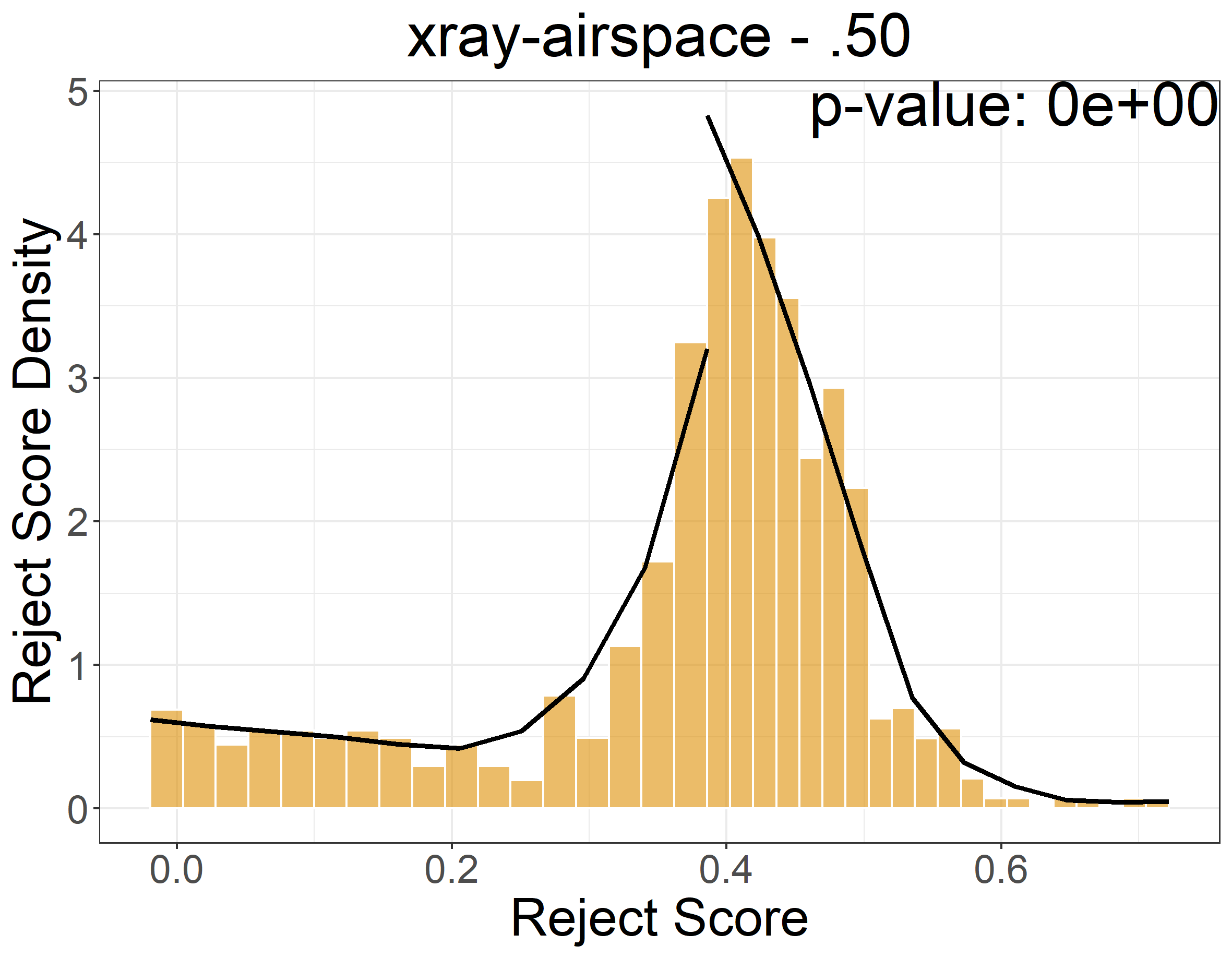
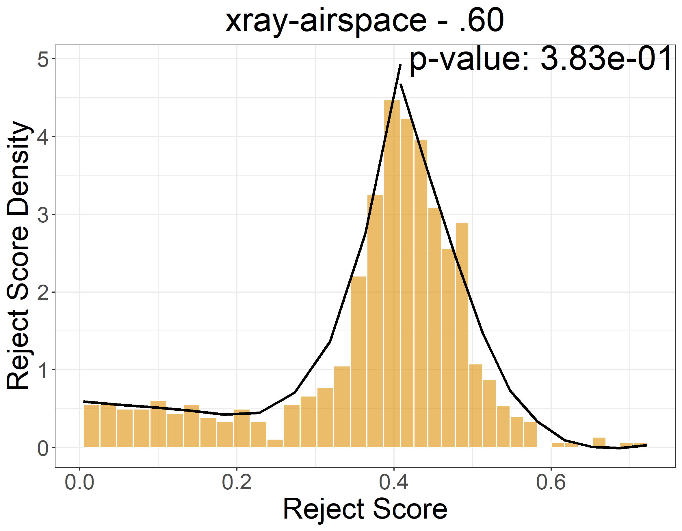
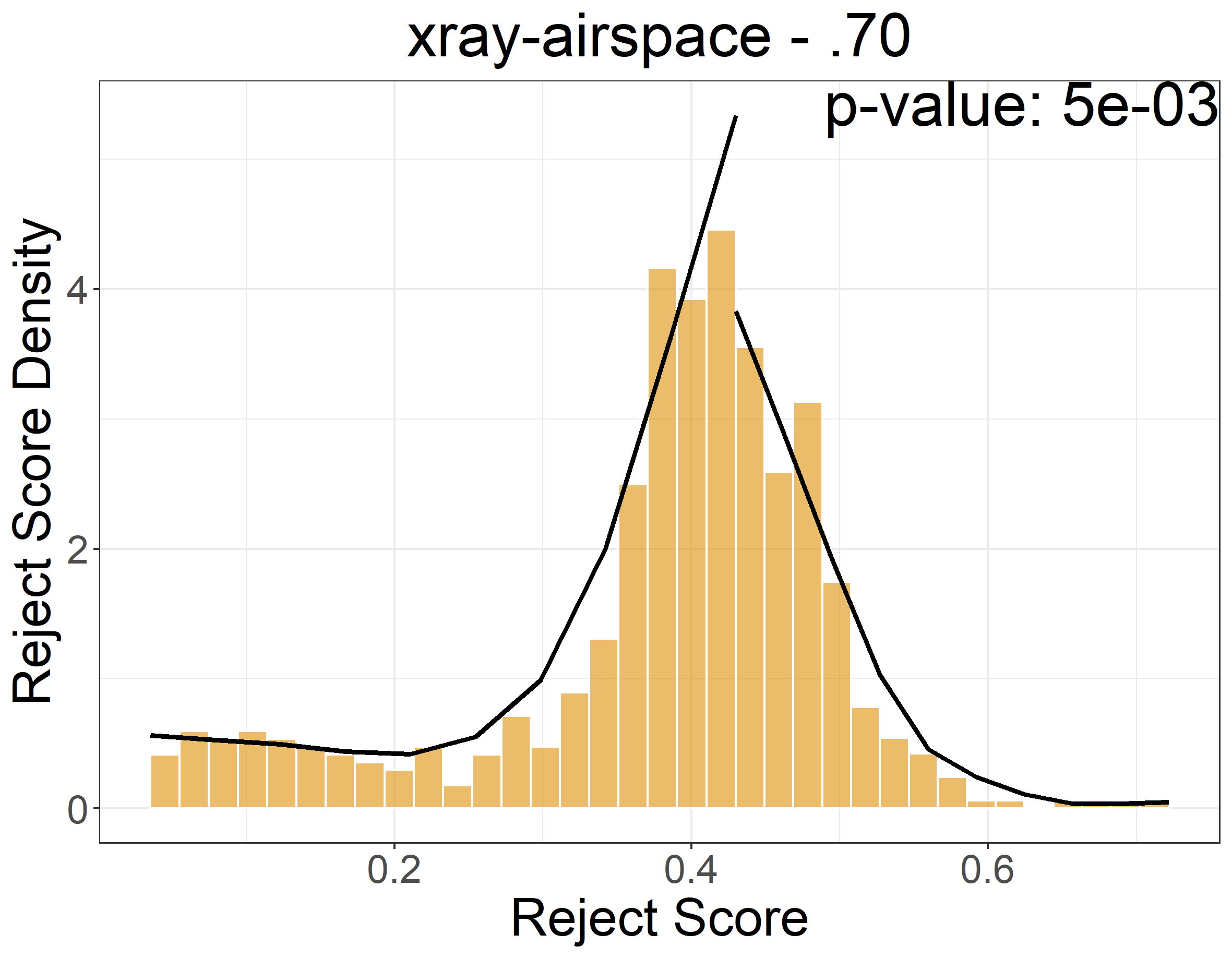
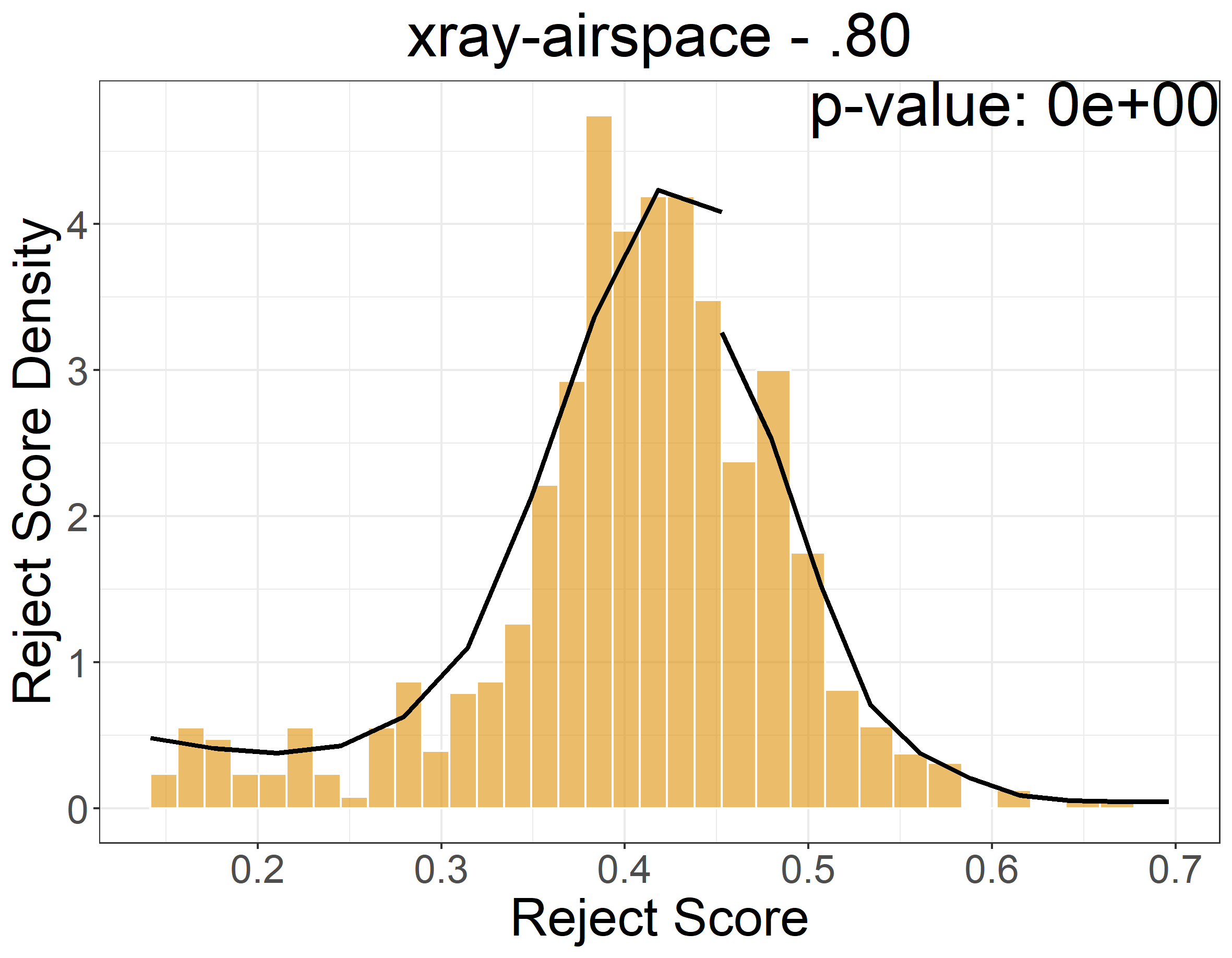
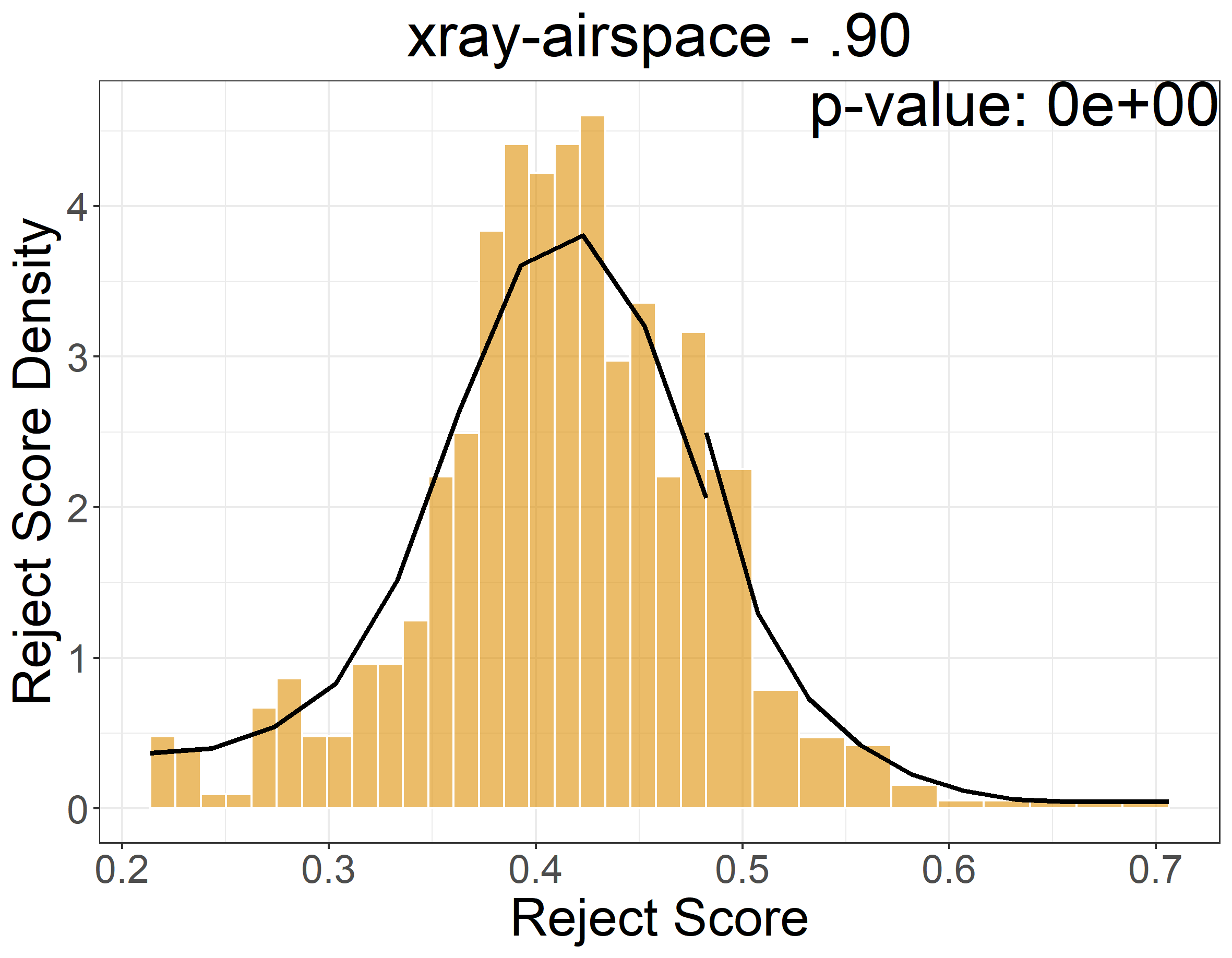
Non-manipulation of the running variable. One instance in which Assumption 1 does not hold is when units know the rule with which the running variable Kisubscript𝐾𝑖K_{i} is computed and/or can manipulate its value. Accordingly, a feasible falsification test involves checking whether the empirical probability distribution of the running variable is smooth (i.e., it does not jump) at the cutoff. This test can be formally conducted by estimating the density of the running variable with histograms or kernel density estimators [91, 92]. For a practical example, see Section D.3 and Figures 7-11.

No effect on predetermined features and placebo outcomes. In a similar spirit to what we described above, another falsification test involves comparing treated and control units near the cutoff to see if they share similar observable traits: if units can’t manipulate their score, there should not be systematic differences between units close to the cutoff, aside from their treatment status. As such, units just above and below the cutoff should resemble each other in all aspects unaffected by the treatment. These aspects (or features) can be predetermined features, variables realizing before treatment assignment, or placebo outcomes, variables that should not have been influenced by the treatment. This test can be conducted by estimating an RD where the outcome variable is either a predetermined feature or a placebo outcome and checking that the null hypothesis of no effect is not rejected. An application of this falsification test can be found in Section D.3.1 and in the fourth row of Figure 6.

Placebo cutoffs. Another type of falsification test involves checking if statistically significant treatment effects can be estimated using artificial cutoff values. We stress that the evidence of no effect –hence smoothness of the expected potential outcomes– away from the cutoff is neither sufficient nor necessary for Assumption 1 to hold, but the presence of discontinuities in other places might discredit such an assumption. To conduct such a test, one has to estimate the RD using a cutoff value that is different from the original one. Section D.3.1 and the second and third rows of Figure 6 showcase this falsification test in our empirical applications.

Optimal coverage

We again stress that RD designs are local in nature. Hence, under Scenario 2, without imposing additional strong parametric assumptions on the shape of 𝔼[T(d)|K=k],d{0,1}𝔼delimited-[]conditional𝑇𝑑𝐾𝑘𝑑01\mathbb{E}[T(d)|K=k],d\in\{0,1\}, we cannot recover the average treatment effect for coverage levels other than κ¯csubscript¯𝜅𝑐\overline{\kappa}_{c}. However, suppose that we have access to different batches of data, where similar human experts and the same ML model take turns in predicting the ground truth Y𝑌Y, but the reject-score threshold was let vary in a countable (ordered) set 𝒦¯𝒦¯𝒦𝒦\overline{\mathcal{K}}\subseteq\mathcal{K}. For instance, we can be in the presence of multiple human moderators that receive different amounts of content to moderate (i.e. κ¯¯𝜅\overline{\kappa} is changing). Then, we can leverage results in the literature of RD designs with multiple non-cumulative cutoffs [93, 94] and identify

τ𝚁𝙳𝙳(k):=𝔼[T(1)T(0)K=k],k[κ¯𝚕𝚋,κ¯𝚞𝚋],formulae-sequenceassignsubscript𝜏𝚁𝙳𝙳𝑘𝔼delimited-[]𝑇1conditional𝑇0𝐾𝑘𝑘subscript¯𝜅𝚕𝚋subscript¯𝜅𝚞𝚋\tau_{\mathtt{RDD}}(k):=\mathbb{E}[T(1)-T(0)\mid K=k],\qquad k\in[\overline{\kappa}_{\mathtt{lb}},\overline{\kappa}_{\mathtt{ub}}],

where κ¯𝚕𝚋:=min𝒦¯assignsubscript¯𝜅𝚕𝚋¯𝒦\overline{\kappa}_{\mathtt{lb}}:=\min\overline{\mathcal{K}} and κ¯𝚞𝚋:=max𝒦¯assignsubscript¯𝜅𝚞𝚋¯𝒦\overline{\kappa}_{\mathtt{ub}}:=\max\overline{\mathcal{K}}. More precisely, identification of τ𝙰𝚃𝙳(k)subscript𝜏𝙰𝚃𝙳𝑘\tau_{\mathtt{ATD}}(k) requires continuity of 𝔼[T(d)K=k],d{0,1}𝔼delimited-[]conditional𝑇𝑑𝐾𝑘𝑑01\mathbb{E}[T(d)\mid K=k],d\in\{0,1\} in k𝑘k for k[κ¯𝚕𝚋,κ¯𝚞𝚋]𝑘subscript¯𝜅𝚕𝚋subscript¯𝜅𝚞𝚋k\in[\overline{\kappa}_{\mathtt{lb}},\overline{\kappa}_{\mathtt{ub}}] and a similar shape of 𝔼[T(0)Ki=k]𝔼delimited-[]conditional𝑇0subscript𝐾𝑖𝑘\mathbb{E}[T(0)\mid K_{i}=k] across datasets. An exercise in this spirit might be useful to choose the optimal level of coverage κ¯:=argmaxk𝒦¯τ𝙰𝚃𝙳(k)assignsuperscript¯𝜅subscriptargmax𝑘¯𝒦subscript𝜏𝙰𝚃𝙳𝑘\overline{\kappa}^{\star}:=\operatorname*{arg\,max}_{k\in\overline{\mathcal{K}}}\tau_{\mathtt{ATD}}(k), where the optimality is defined in the sense of getting the largest increase in predictive accuracy out of having human experts guessing instead of the model.

Should we increase or decrease the coverage?

Despite being local by construction, the RD can be used to learn about the gradient of the treatment effect at the cutoff. Indeed, Dong and Lewbel [95] show that, under regularity conditions on how 𝔼[T(d)K=k],d{0,1}𝔼delimited-[]conditional𝑇𝑑𝐾𝑘𝑑01\mathbb{E}[T(d)\mid K=k],d\in\{0,1\} changes around κ¯csubscript¯𝜅𝑐\overline{\kappa}_{c}, the RD setting can be used to learn how τ𝚁𝙳subscript𝜏𝚁𝙳\tau_{\mathtt{RD}} would change if the reject-score threshold κ¯csubscript¯𝜅𝑐\overline{\kappa}_{c} were marginally changed. Therefore, this suggests that when the deferring system accuracy is maximal, τ𝚁𝙳subscript𝜏𝚁𝙳\tau_{\mathtt{RD}} should be close to zero. The intuition is that we should be indifferent between predicting with the ML model or deferring to the human expert at the optimal value.

Uncertainty in the ML model estimation

The outcome variable for unit i𝑖i in the LtD framework is Ti=𝟙{ϑ(𝐗i)=Yi}subscript𝑇𝑖1italic-ϑsubscript𝐗𝑖subscript𝑌𝑖T_{i}=\mathds{1}\{\vartheta(\mathbf{X}_{i})=Y_{i}\} and the running variable is the reject score Ki=k(𝐗i)subscript𝐾𝑖𝑘subscript𝐗𝑖K_{i}=k(\mathbf{X}_{i}) (see Table 1). However, in practice, we compute the outcome and the reject score via an estimated version of the model, i.e. f^().^𝑓\hat{f}(\cdot). We explicitly do not consider this source of uncertainty because access is usually limited to an estimated final version of the model without possibly fitting it again (e.g., large language models [96]). For this reason, with a slight abuse of notation, we always write f()𝑓f(\cdot), Tisubscript𝑇𝑖T_{i}, and Kisubscript𝐾𝑖K_{i} when we should write f^()^𝑓\hat{f}(\cdot), T^i,subscript^𝑇𝑖\hat{T}_{i}, and K^isubscript^𝐾𝑖\hat{K}_{i}, respectively. If one is willing also to capture this uncertainty and model re-estimation is viable, off-the-shelf non-parametric bootstrap procedures are available. Moreover, [97] show that under the condition that the noisy score correctly assigns samples to treatment and control groups, τ𝚁𝙳subscript𝜏𝚁𝙳\tau_{\mathtt{RD}} can be interpreted as the treatment effect when the noisy score equals the cutoff. We argue that this latter measure is still the one of interest, particularly so when the model is taken as given because the reject score can only be computed using the estimated ML model.

Appendix D Experimental evaluation

D.1 Additional details

D.1.1 Data

We use the data from Mozannar et al. [7] and Okati et al. [2].

Concerning the synthetic dataset synth, we generate the data using the method described in Mozannar et al. [7]333See the GitHub repository https://github.com/clinicalml/human_ai_deferral: given a parameter d𝑑d, 𝐱d𝐱superscript𝑑\mathbf{x}\in\mathbb{R}^{d} is sampled from a mixture of d𝑑d equally weighted Gaussians, each one with uniformly random mean and variance. To obtain the target variable Y𝑌Y, the procedure generates two random half-spaces, one referring to the optimal policy function g:𝒳{0,1}:superscript𝑔𝒳01g^{*}:\mathcal{X}\to\{0,1\} and one representing an optimal ML model f:𝒳𝒴:superscript𝑓𝒳𝒴f^{*}:\mathcal{X}\to\mathcal{Y}. The fraction of instances for which g(𝐱)=0superscript𝑔𝐱0g^{*}(\mathbf{x})=0 is randomly chosen to be between .20.20.20 and .80.80.80. For all those instances on the side where g(𝐱)=0superscript𝑔𝐱0g^{*}(\mathbf{x})=0, the target variable Y𝑌Y is changed to be consistent with the optimal ML model f(𝐱)superscript𝑓𝐱f^{*}(\mathbf{x}) with probability 1pML1subscript𝑝𝑀𝐿1-p_{ML} and otherwise uniform. Conversely, when g(𝐗)=1superscript𝑔𝐗1g^{*}(\mathbf{X})=1, the labels are uniformly sampled. The human expert h(𝐱)𝐱h(\mathbf{x}) is then set to make mistakes at a rate of ph0subscript𝑝0p_{h0} when g(𝐱)=0superscript𝑔𝐱0g^{*}(\mathbf{x})=0 and at a rate of ph1subscript𝑝1p_{h1} when g(𝐱)=1superscript𝑔𝐱1g^{*}(\mathbf{x})=1. In our experiments, we set d=30𝑑30d=30, ph0=.30subscript𝑝0.30p_{h0}=.30, ph1=.10subscript𝑝1.10p_{h1}=.10, pML=.20subscript𝑝𝑀𝐿.20p_{ML}=.20.

Regarding real data, in cifar10h [48], the task is to annotate images belonging to 10 different categories. Here, the human prediction is provided by a separate human annotator.

In galaxyzoo [49], the main task is identifying whether the image contains a non-smooth galaxy. Thus, Y=0𝑌0Y=0 if the image contains a smooth galaxy and Y=1𝑌1Y=1 otherwise. Since we have 30 annotators for each image, we consider the majority of the annotators as the target variable Y𝑌Y, while the human expert prediction h(𝐗)𝐗h(\mathbf{X}) is sampled randomly from the 30 annotators.

For hatespeech [50], the goal is to detect whether the text contains offensive or hate-speech language. The human predictor is sampled randomly as in Mozannar et al. [7].

Finally, xray-airspace [51, 52] contains both chest X-rays with human predictions and chest X-rays without human predictions. For each image, the target variable Y𝑌Y encodes the presence of an airspace opacity. The human predictions are randomly sampled from multiple experts, as done by Mozannar et al. [7].

D.1.2 Baselines

Selective Prediction (SP): Geifman and El-Yaniv [53] present a neural network classifier with a reject option. The reject score is defined considering the maximum of the final softmax values, i.e., k(𝐱)=maxysy(𝐱)𝑘𝐱subscript𝑦subscript𝑠𝑦𝐱k(\mathbf{x})=\max_{y}s_{y}(\mathbf{x}), where sy(𝐱)subscript𝑠𝑦𝐱s_{y}(\mathbf{x}) is the final layer softmax value for class y𝑦y. We stress that SP does not take into account the human expert’s ability but determines deferral only based on those cases where the ML model is uncertain.

Compare Confidence (CC): Raghu et al. [3] extend SP by learning (independently) another model - called the expert model - that uses as a target variable whether the human expert is correct. Then, deferral is determined by comparing the reject score of the classifier and the expert model.

Differentiable Triage (DT): Okati et al. [2] consider a two-stage approach, where at each epoch (i) the classifier is trained only on those points where the classifier loss is lower than the human loss, (ii) another ML model - called the rejector - is fitted to predict who has a lower loss between the classifier and the human. At the end of the training procedure, deferral is decided based on the estimated probability of the human expert having a lower loss than the classifier.

Cross-Entropy Surrogate (LCE): Mozannar and Sontag [4] propose a consistent surrogate loss of (2), when l𝑙l is the 0-1 loss. The surrogate loss is then used to train the deferring system, which employs a neural network with an additional head to represent deferral;

One Vs All (OVA): Verma and Nalisnick [5] propose a different consistent surrogate loss, which improves the final calibration of the deferring system;

Realizable Surrogate (RS): Mozannar et al. [7] extend the approaches based on surrogate losses by considering a consistent and realizable-consistent surrogate of (2), when lMsubscript𝑙𝑀l_{M} and lHsubscript𝑙𝐻l_{H} are the 0-1 loss. As for LCE, also RS considers a neural network with an additional head representing deferral.

Asymmetric SoftMax (ASM): Cao et al. [8] extend both LCE and OVA by providing a surrogate loss that ensures a better calibration of the reject score.

For all the baselines but ASM, we consider the implementation provided by Mozannar et al. [7]3. We implement ASM from Cao et al. [8]’s code, which can be found in their supplementary material.

D.1.3 Hyperparameters

For synth, we considered a simple linear feedforward architecture. For each baseline, we trained the model for 505050 epochs with lr=1e2lr1𝑒2\texttt{lr}=1e-2 and Adam [98] as the optimizer. Batch size was set to 1,02410241,024.

For real data, all the methods were trained following the settings in either Mozannar et al. [7] (cifar10h, hatespeech, xray-airspace) or Okati et al. [2] (galaxyzoo).

In particular, for cifar10h, we trained a base WideResNet on the original cifar10 dataset for 200 epochs using cross-entropy loss, learning rate equals to .001.001.001 and AdamW [99] as an optimizer. For each baseline, we fine-tuned the base WideResnet on cifar10h for 150 epochs, using a learning rate of .001.001.001 and AdamW as an optimizer.

For hatespeech, we considered pre-trained embeddings of SBERT and we fine-tuned a feed-forward neural network for 100 epochs, setting the learning rate to .01.01.01 and Adam as optimizer.

For xray-airspace, we first fine-tuned a pre-trained DenseNet121 [47] for 10 epochs on the x-rays that do not contain human predictions, setting lr=1e4lr1E-4\texttt{lr}=$110-4$ and AdamW as the optimizer. For each baseline, we further fine-tuned the obtained model, training it for 333 epochs on xray-airspace with a learning rate equal to 1e31E-3110-3 and AdamW as the optimizer.

Finally, for galaxyzoo, we consider a pre-trained ResNet50 and train each baseline for 505050 epochs, using Adam as the optimizer and a learning rate of 1e31E-3110-3.

The batch size was set to 128128128 for all the real datasets.

D.1.4 Hardware and carbon footprint

Regarding computational resources, we split the workload over two machines: (i)𝑖(i) a 96 cores machine with Intel(R) Xeon(R) Gold 6342 CPU @ 2.80GHz and two NVIDIA RTX A6000, OS Ubuntu 20.04.4; (ii)𝑖𝑖(ii) a 224 cores machine with Intel(R) Xeon(R) Platinum 8480+ CPU and eight NVIDIA A100-SXM4-80GB, OS Ubuntu 22.04.4 LTS.

We track all our runs using the Python package codecarbon [100]. This allows us to consider the total time required by all our experimentation (including failed and repeated experiments) and its environmental costs. Overall, the cumulated time of all our runs amounts to 5absent5\approx 5 days. This translates into an overall CO2subscriptCO2\text{CO}_{2} consumption of roughly 25.2absent25.2\approx 25.2 Kg Eq.CO2subscriptCO2\text{CO}_{2}, which equals a car drive of 60absent60\approx 60 miles.

D.2 Detailed results for Q1, Q2 and Q3

Tables 3-7 report the detailed results of experiments on the synthetic and the real datasets. Tables include τ^𝙰𝚃𝙳subscript^𝜏𝙰𝚃𝙳\hat{\tau}_{\mathtt{ATD}} (the Scenario 1 main estimate), τ^𝚁𝙳subscript^𝜏𝚁𝙳\hat{\tau}_{\mathtt{RD}} (the Scenario 2 main estimate), and the deferring system accuracy at various target coverages for all the seven baselines. For τ^𝙰𝚃𝙳subscript^𝜏𝙰𝚃𝙳\hat{\tau}_{\mathtt{ATD}} and τ^𝚁𝙳subscript^𝜏𝚁𝙳\hat{\tau}_{\mathtt{RD}}, we show in parentheses the associated p-value when testing the significance of the causal effect being different from zero. Significant (after Bonferroni correction of α=0.05𝛼0.05\alpha=0.05) p-values are shown in blue.

Q3: real datasets under Scenario 2. We observe that most of the τ^𝚁𝙳subscript^𝜏𝚁𝙳\hat{\tau}_{\mathtt{RD}} estimates are not statistically significant. A motivation for this is because the considered test sets are not large in size, ranging from 854854854 (xray-airspace) to 4,59745974,597 (hatespeech) instances. This impacts the estimation strategy, as τ^𝚁𝙳subscript^𝜏𝚁𝙳\hat{\tau}_{\mathtt{RD}} is computed through local kernel regressions over instances within an optimal bandwidth. In summary, locally to the deferring boundary, the difference between the ML model and the human expert is minimal (we cannot reject the null hypothesis that it is zero) for most of the coverages c𝑐c.

A few exceptions can be noticed. For galaxyzoo and the CC baseline, a few statistically significant (and negative) effects on τ^𝚁𝙳subscript^𝜏𝚁𝙳\hat{\tau}_{\mathtt{RD}} occur. The ML model performs generally better than the human expert on this task, advocating for almost full automation. For hatespeech, there is a statistically significant effect .348(pv4.1e5)absent.348𝑝𝑣4.1E-5\approx.348~{}(pv\approx$4.110-5$) for RS (the best baseline w.r.t. accuracy) at κ¯c=.90subscript¯𝜅𝑐.90\overline{\kappa}_{c}=.90. Thus, the causal effect of deferring to the human expert on instances around the cutoff κ¯.90subscript¯𝜅.90\overline{\kappa}_{.90} is positive. For xray-airspace, which resembles the settings of the example (Ex2) from the introduction, and for the RS baseline, there is at κ¯.30subscript¯𝜅.30\overline{\kappa}_{.30} a large negative effect effect of .473absent.473\approx-.473 (pv8.95e3𝑝𝑣8.95E-3pv\approx$8.9510-3$, yet not statistically significant). This is in favor of deferring from the human expert to the ML model.

We also notice some extreme cases where there is insufficient variability of the reject scores at the cutoff. This occurs when the reject scores are peaked around a value. In those cases, the local polynomial regression, as implemented by rdrobust, is not able to estimate τ^𝚁𝙳subscript^𝜏𝚁𝙳\hat{\tau}_{\mathtt{RD}}. These cases are reported as “-” in Tables 3-7.

Table 3: synth results. Bold for highest value, blue p-values for statistical significance.
c𝑐c ASM CC DT LCE OVA RS SP
τ^𝙰𝚃𝙳subscript^𝜏𝙰𝚃𝙳\hat{\tau}_{\mathtt{ATD}} .00 .095(6.98e26).0956.98E-26.095~{}({\color[rgb]{0,0,1}\definecolor[named]{pgfstrokecolor}{rgb}{0,0,1}$6.9810-26$}) .128(1.07e45).1281.07E-45.128~{}({\color[rgb]{0,0,1}\definecolor[named]{pgfstrokecolor}{rgb}{0,0,1}$1.0710-45$}) .112(1.66e35).1121.66E-35.112~{}({\color[rgb]{0,0,1}\definecolor[named]{pgfstrokecolor}{rgb}{0,0,1}$1.6610-35$}) .123(1.07e42).1231.07E-42.123~{}({\color[rgb]{0,0,1}\definecolor[named]{pgfstrokecolor}{rgb}{0,0,1}$1.0710-42$}) .122(2.63e42).1222.63E-42.122~{}({\color[rgb]{0,0,1}\definecolor[named]{pgfstrokecolor}{rgb}{0,0,1}$2.6310-42$}) .098(1.10e27).0981.10E-27.098~{}({\color[rgb]{0,0,1}\definecolor[named]{pgfstrokecolor}{rgb}{0,0,1}$1.1010-27$}) .132(1.55e𝟒𝟖).1321.55E-48\mathbf{.132~{}({\color[rgb]{0,0,1}\definecolor[named]{pgfstrokecolor}{rgb}{0,0,1}$1.5510-48$})}
.10 .127(3.53e40).1273.53E-40.127~{}({\color[rgb]{0,0,1}\definecolor[named]{pgfstrokecolor}{rgb}{0,0,1}$3.5310-40$}) .164(1.53e𝟔𝟓).1641.53E-65\mathbf{.164~{}({\color[rgb]{0,0,1}\definecolor[named]{pgfstrokecolor}{rgb}{0,0,1}$1.5310-65$})} .137(1.29e46).1371.29E-46.137~{}({\color[rgb]{0,0,1}\definecolor[named]{pgfstrokecolor}{rgb}{0,0,1}$1.2910-46$}) .154(8.57e59).1548.57E-59.154~{}({\color[rgb]{0,0,1}\definecolor[named]{pgfstrokecolor}{rgb}{0,0,1}$8.5710-59$}) .154(8.23e59).1548.23E-59.154~{}({\color[rgb]{0,0,1}\definecolor[named]{pgfstrokecolor}{rgb}{0,0,1}$8.2310-59$}) .130(1.27e41).1301.27E-41.130~{}({\color[rgb]{0,0,1}\definecolor[named]{pgfstrokecolor}{rgb}{0,0,1}$1.2710-41$}) .158(2.83e62).1582.83E-62.158~{}({\color[rgb]{0,0,1}\definecolor[named]{pgfstrokecolor}{rgb}{0,0,1}$2.8310-62$})
.20 .159(1.28e55).1591.28E-55.159~{}({\color[rgb]{0,0,1}\definecolor[named]{pgfstrokecolor}{rgb}{0,0,1}$1.2810-55$}) .191(9.98e𝟖𝟏).1919.98E-81\mathbf{.191~{}({\color[rgb]{0,0,1}\definecolor[named]{pgfstrokecolor}{rgb}{0,0,1}$9.9810-81$})} .164(1.01e59).1641.01E-59.164~{}({\color[rgb]{0,0,1}\definecolor[named]{pgfstrokecolor}{rgb}{0,0,1}$1.0110-59$}) .178(1.57e70).1781.57E-70.178~{}({\color[rgb]{0,0,1}\definecolor[named]{pgfstrokecolor}{rgb}{0,0,1}$1.5710-70$}) .188(6.60e80).1886.60E-80.188~{}({\color[rgb]{0,0,1}\definecolor[named]{pgfstrokecolor}{rgb}{0,0,1}$6.6010-80$}) .166(7.48e61).1667.48E-61.166~{}({\color[rgb]{0,0,1}\definecolor[named]{pgfstrokecolor}{rgb}{0,0,1}$7.4810-61$}) .179(4.01e72).1794.01E-72.179~{}({\color[rgb]{0,0,1}\definecolor[named]{pgfstrokecolor}{rgb}{0,0,1}$4.0110-72$})
.30 .205(7.92e81).2057.92E-81.205~{}({\color[rgb]{0,0,1}\definecolor[named]{pgfstrokecolor}{rgb}{0,0,1}$7.9210-81$}) .229(1.58e𝟏𝟎𝟎).2291.58E-100\mathbf{.229~{}({\color[rgb]{0,0,1}\definecolor[named]{pgfstrokecolor}{rgb}{0,0,1}$1.5810-100$})} .198(2.65e76).1982.65E-76.198~{}({\color[rgb]{0,0,1}\definecolor[named]{pgfstrokecolor}{rgb}{0,0,1}$2.6510-76$}) .203(1.90e81).2031.90E-81.203~{}({\color[rgb]{0,0,1}\definecolor[named]{pgfstrokecolor}{rgb}{0,0,1}$1.9010-81$}) .223(1.55e97).2231.55E-97.223~{}({\color[rgb]{0,0,1}\definecolor[named]{pgfstrokecolor}{rgb}{0,0,1}$1.5510-97$}) .202(2.14e78).2022.14E-78.202~{}({\color[rgb]{0,0,1}\definecolor[named]{pgfstrokecolor}{rgb}{0,0,1}$2.1410-78$}) .208(2.51e86).2082.51E-86.208~{}({\color[rgb]{0,0,1}\definecolor[named]{pgfstrokecolor}{rgb}{0,0,1}$2.5110-86$})
.40 .262(6.27e116).2626.27E-116.262~{}({\color[rgb]{0,0,1}\definecolor[named]{pgfstrokecolor}{rgb}{0,0,1}$6.2710-116$}) .264(5.01e𝟏𝟏𝟕).2645.01E-117\mathbf{.264~{}({\color[rgb]{0,0,1}\definecolor[named]{pgfstrokecolor}{rgb}{0,0,1}$5.0110-117$})} .234(4.86e92).2344.86E-92.234~{}({\color[rgb]{0,0,1}\definecolor[named]{pgfstrokecolor}{rgb}{0,0,1}$4.8610-92$}) .234(8.99e95).2348.99E-95.234~{}({\color[rgb]{0,0,1}\definecolor[named]{pgfstrokecolor}{rgb}{0,0,1}$8.9910-95$}) .262(7.11e118).2627.11E-118.262~{}({\color[rgb]{0,0,1}\definecolor[named]{pgfstrokecolor}{rgb}{0,0,1}$7.1110-118$}) .251(9.56e106).2519.56E-106.251~{}({\color[rgb]{0,0,1}\definecolor[named]{pgfstrokecolor}{rgb}{0,0,1}$9.5610-106$}) .233(2.39e94).2332.39E-94.233~{}({\color[rgb]{0,0,1}\definecolor[named]{pgfstrokecolor}{rgb}{0,0,1}$2.3910-94$})
.50 .320(9.03e𝟏𝟓𝟖).3209.03E-158\mathbf{.320~{}({\color[rgb]{0,0,1}\definecolor[named]{pgfstrokecolor}{rgb}{0,0,1}$9.0310-158$})} .305(1.16e138).3051.16E-138.305~{}({\color[rgb]{0,0,1}\definecolor[named]{pgfstrokecolor}{rgb}{0,0,1}$1.1610-138$}) .260(1.51e98).2601.51E-98.260~{}({\color[rgb]{0,0,1}\definecolor[named]{pgfstrokecolor}{rgb}{0,0,1}$1.5110-98$}) .260(9.15e98).2609.15E-98.260~{}({\color[rgb]{0,0,1}\definecolor[named]{pgfstrokecolor}{rgb}{0,0,1}$9.1510-98$}) .302(6.62e136).3026.62E-136.302~{}({\color[rgb]{0,0,1}\definecolor[named]{pgfstrokecolor}{rgb}{0,0,1}$6.6210-136$}) .319(7.30e150).3197.30E-150.319~{}({\color[rgb]{0,0,1}\definecolor[named]{pgfstrokecolor}{rgb}{0,0,1}$7.3010-150$}) .248(3.62e88).2483.62E-88.248~{}({\color[rgb]{0,0,1}\definecolor[named]{pgfstrokecolor}{rgb}{0,0,1}$3.6210-88$})
.60 .375(2.62e𝟏𝟖𝟏).3752.62E-181\mathbf{.375~{}({\color[rgb]{0,0,1}\definecolor[named]{pgfstrokecolor}{rgb}{0,0,1}$2.6210-181$})} .335(2.03e137).3352.03E-137.335~{}({\color[rgb]{0,0,1}\definecolor[named]{pgfstrokecolor}{rgb}{0,0,1}$2.0310-137$}) .291(3.45e104).2913.45E-104.291~{}({\color[rgb]{0,0,1}\definecolor[named]{pgfstrokecolor}{rgb}{0,0,1}$3.4510-104$}) .289(1.83e99).2891.83E-99.289~{}({\color[rgb]{0,0,1}\definecolor[named]{pgfstrokecolor}{rgb}{0,0,1}$1.8310-99$}) .347(5.46e155).3475.46E-155.347~{}({\color[rgb]{0,0,1}\definecolor[named]{pgfstrokecolor}{rgb}{0,0,1}$5.4610-155$}) .363(8.52e170).3638.52E-170.363~{}({\color[rgb]{0,0,1}\definecolor[named]{pgfstrokecolor}{rgb}{0,0,1}$8.5210-170$}) .264(7.92e82).2647.92E-82.264~{}({\color[rgb]{0,0,1}\definecolor[named]{pgfstrokecolor}{rgb}{0,0,1}$7.9210-82$})
.70 .404(8.12e𝟏𝟔𝟏).4048.12E-161\mathbf{.404~{}({\color[rgb]{0,0,1}\definecolor[named]{pgfstrokecolor}{rgb}{0,0,1}$8.1210-161$})} .364(3.09e127).3643.09E-127.364~{}({\color[rgb]{0,0,1}\definecolor[named]{pgfstrokecolor}{rgb}{0,0,1}$3.0910-127$}) .323(3.13e99).3233.13E-99.323~{}({\color[rgb]{0,0,1}\definecolor[named]{pgfstrokecolor}{rgb}{0,0,1}$3.1310-99$}) .327(1.28e101).3271.28E-101.327~{}({\color[rgb]{0,0,1}\definecolor[named]{pgfstrokecolor}{rgb}{0,0,1}$1.2810-101$}) .381(6.66e148).3816.66E-148.381~{}({\color[rgb]{0,0,1}\definecolor[named]{pgfstrokecolor}{rgb}{0,0,1}$6.6610-148$}) .390(4.27e155).3904.27E-155.390~{}({\color[rgb]{0,0,1}\definecolor[named]{pgfstrokecolor}{rgb}{0,0,1}$4.2710-155$}) .281(1.17e69).2811.17E-69.281~{}({\color[rgb]{0,0,1}\definecolor[named]{pgfstrokecolor}{rgb}{0,0,1}$1.1710-69$})
.80 .409(4.07e𝟏𝟎𝟔).4094.07E-106\mathbf{.409~{}({\color[rgb]{0,0,1}\definecolor[named]{pgfstrokecolor}{rgb}{0,0,1}$4.0710-106$})} .378(1.31e94).3781.31E-94.378~{}({\color[rgb]{0,0,1}\definecolor[named]{pgfstrokecolor}{rgb}{0,0,1}$1.3110-94$}) .340(1.98e72).3401.98E-72.340~{}({\color[rgb]{0,0,1}\definecolor[named]{pgfstrokecolor}{rgb}{0,0,1}$1.9810-72$}) .357(1.04e83).3571.04E-83.357~{}({\color[rgb]{0,0,1}\definecolor[named]{pgfstrokecolor}{rgb}{0,0,1}$1.0410-83$}) .386(2.32e100).3862.32E-100.386~{}({\color[rgb]{0,0,1}\definecolor[named]{pgfstrokecolor}{rgb}{0,0,1}$2.3210-100$}) .375(7.04e89).3757.04E-89.375~{}({\color[rgb]{0,0,1}\definecolor[named]{pgfstrokecolor}{rgb}{0,0,1}$7.0410-89$}) .293(1.06e51).2931.06E-51.293~{}({\color[rgb]{0,0,1}\definecolor[named]{pgfstrokecolor}{rgb}{0,0,1}$1.0610-51$})
.90 .417(7.32e58).4177.32E-58.417~{}({\color[rgb]{0,0,1}\definecolor[named]{pgfstrokecolor}{rgb}{0,0,1}$7.3210-58$}) .421(8.99e𝟔𝟏).4218.99E-61\mathbf{.421~{}({\color[rgb]{0,0,1}\definecolor[named]{pgfstrokecolor}{rgb}{0,0,1}$8.9910-61$})} .376(3.83e42).3763.83E-42.376~{}({\color[rgb]{0,0,1}\definecolor[named]{pgfstrokecolor}{rgb}{0,0,1}$3.8310-42$}) .358(5.77e40).3585.77E-40.358~{}({\color[rgb]{0,0,1}\definecolor[named]{pgfstrokecolor}{rgb}{0,0,1}$5.7710-40$}) .385(1.88e55).3851.88E-55.385~{}({\color[rgb]{0,0,1}\definecolor[named]{pgfstrokecolor}{rgb}{0,0,1}$1.8810-55$}) .389(3.32e46).3893.32E-46.389~{}({\color[rgb]{0,0,1}\definecolor[named]{pgfstrokecolor}{rgb}{0,0,1}$3.3210-46$}) .308(2.61e30).3082.61E-30.308~{}({\color[rgb]{0,0,1}\definecolor[named]{pgfstrokecolor}{rgb}{0,0,1}$2.6110-30$})
τ^𝚁𝙳subscript^𝜏𝚁𝙳\hat{\tau}_{\mathtt{RD}} .10 .184(3.62e3).1843.62E-3-.184~{}($3.6210-3$) .146(4.69e2).1464.69E-2-.146~{}($4.6910-2$) .095(1.21e1).0951.21E-1-.095~{}($1.2110-1$) .130(6.87e2).1306.87E-2-.130~{}($6.8710-2$) .156(7.23e2).1567.23E-2-.156~{}($7.2310-2$) .272(2.83e3).2722.83E-3-.272~{}($2.8310-3$) .068(5.10e𝟏).0685.10E-1\mathbf{.068~{}($5.1010-1$)}
.20 .246(4.21e4).2464.21E-4-.246~{}($4.2110-4$) .183(9.61e3).1839.61E-3-.183~{}($9.6110-3$) .107(3.22e2).1073.22E-2-.107~{}($3.2210-2$) .034(4.94e1).0344.94E-1-.034~{}($4.9410-1$) .044(5.02e1).0445.02E-1-.044~{}($5.0210-1$) .086(1.54e1).0861.54E-1-.086~{}($1.5410-1$) .117(1.57e𝟏).1171.57E-1\mathbf{.117~{}($1.5710-1$)}
.30 .052(4.57e1).0524.57E-1-.052~{}($4.5710-1$) .008(8.73e𝟏).0088.73E-1\mathbf{.008~{}($8.7310-1$)} .015(7.74e1).0157.74E-1-.015~{}($7.7410-1$) .012(8.31e1).0128.31E-1-.012~{}($8.3110-1$) .077(1.69e1).0771.69E-1-.077~{}($1.6910-1$) .098(1.15e1).0981.15E-1-.098~{}($1.1510-1$) .158(1.54e2).1581.54E-2-.158~{}($1.5410-2$)
.40 .272(3.14e2).2723.14E-2-.272~{}($3.1410-2$) .051(2.78e1).0512.78E-1-.051~{}($2.7810-1$) .009(8.45e1).0098.45E-1-.009~{}($8.4510-1$) .099(9.91e2).0999.91E-2.099~{}($9.9110-2$) .007(9.08e1).0079.08E-1.007~{}($9.0810-1$) .126(5.03e2).1265.03E-2-.126~{}($5.0310-2$) .106(7.09e𝟐).1067.09E-2\mathbf{.106~{}($7.0910-2$)}
.50 .045(6.72e1).0456.72E-1.045~{}($6.7210-1$) .080(1.46e1).0801.46E-1.080~{}($1.4610-1$) .113(3.47e2).1133.47E-2.113~{}($3.4710-2$) .053(3.94e1).0533.94E-1.053~{}($3.9410-1$) .134(2.31e2).1342.31E-2.134~{}($2.3110-2$) .024(6.39e1).0246.39E-1-.024~{}($6.3910-1$) .190(1.28e𝟑).1901.28E-3\mathbf{.190~{}($1.2810-3$)}
.60 .022(8.26e1).0228.26E-1-.022~{}($8.2610-1$) .096(1.72e1).0961.72E-1.096~{}($1.7210-1$) .149(1.47e2).1491.47E-2.149~{}($1.4710-2$) .147(1.81e2).1471.81E-2.147~{}($1.8110-2$) .328(3.55e6).3283.55E-6.328~{}({\color[rgb]{0,0,1}\definecolor[named]{pgfstrokecolor}{rgb}{0,0,1}$3.5510-6$}) .340(3.76e𝟔).3403.76E-6\mathbf{.340~{}({\color[rgb]{0,0,1}\definecolor[named]{pgfstrokecolor}{rgb}{0,0,1}$3.7610-6$})} .240(9.45e4).2409.45E-4.240~{}($9.4510-4$)
.70 .417(5.28e𝟏𝟎).4175.28E-10\mathbf{.417~{}({\color[rgb]{0,0,1}\definecolor[named]{pgfstrokecolor}{rgb}{0,0,1}$5.2810-10$})} .314(5.59e7).3145.59E-7.314~{}({\color[rgb]{0,0,1}\definecolor[named]{pgfstrokecolor}{rgb}{0,0,1}$5.5910-7$}) .210(4.80e4).2104.80E-4.210~{}($4.8010-4$) .062(3.66e1).0623.66E-1.062~{}($3.6610-1$) .374(1.32e10).3741.32E-10.374~{}({\color[rgb]{0,0,1}\definecolor[named]{pgfstrokecolor}{rgb}{0,0,1}$1.3210-10$}) .339(5.01e7).3395.01E-7.339~{}({\color[rgb]{0,0,1}\definecolor[named]{pgfstrokecolor}{rgb}{0,0,1}$5.0110-7$}) .352(1.71e7).3521.71E-7.352~{}({\color[rgb]{0,0,1}\definecolor[named]{pgfstrokecolor}{rgb}{0,0,1}$1.7110-7$})
.80 .427(1.20e14).4271.20E-14.427~{}({\color[rgb]{0,0,1}\definecolor[named]{pgfstrokecolor}{rgb}{0,0,1}$1.2010-14$}) .370(2.01e7).3702.01E-7.370~{}({\color[rgb]{0,0,1}\definecolor[named]{pgfstrokecolor}{rgb}{0,0,1}$2.0110-7$}) .277(2.63e6).2772.63E-6.277~{}({\color[rgb]{0,0,1}\definecolor[named]{pgfstrokecolor}{rgb}{0,0,1}$2.6310-6$}) .333(7.94e9).3337.94E-9.333~{}({\color[rgb]{0,0,1}\definecolor[named]{pgfstrokecolor}{rgb}{0,0,1}$7.9410-9$}) .429(2.18e𝟏𝟐).4292.18E-12\mathbf{.429~{}({\color[rgb]{0,0,1}\definecolor[named]{pgfstrokecolor}{rgb}{0,0,1}$2.1810-12$})} .236(1.02e3).2361.02E-3.236~{}($1.0210-3$) .170(3.32e2).1703.32E-2.170~{}($3.3210-2$)
.90 .345(1.71e5).3451.71E-5.345~{}({\color[rgb]{0,0,1}\definecolor[named]{pgfstrokecolor}{rgb}{0,0,1}$1.7110-5$}) .460(1.67e𝟏𝟎).4601.67E-10\mathbf{.460~{}({\color[rgb]{0,0,1}\definecolor[named]{pgfstrokecolor}{rgb}{0,0,1}$1.6710-10$})} .418(1.01e5).4181.01E-5.418~{}({\color[rgb]{0,0,1}\definecolor[named]{pgfstrokecolor}{rgb}{0,0,1}$1.0110-5$}) .222(7.58e3).2227.58E-3.222~{}($7.5810-3$) .401(2.28e9).4012.28E-9.401~{}({\color[rgb]{0,0,1}\definecolor[named]{pgfstrokecolor}{rgb}{0,0,1}$2.2810-9$}) .254(4.17e3).2544.17E-3.254~{}($4.1710-3$) .280(1.87e3).2801.87E-3.280~{}($1.8710-3$)
Accuracy .00 .797.797\mathbf{.797} .797.797\mathbf{.797} .797.797\mathbf{.797} .797.797\mathbf{.797} .797.797\mathbf{.797} .797.797\mathbf{.797} .797.797\mathbf{.797}
.10 .817.817\mathbf{.817} .816.816.816 .808.808.808 .812.812.812 .813.813.813 .815.815.815 .809.809.809
.20 .831.831.831 .825.825.825 .818.818.818 .818.818.818 .828.828.828 .833.833\mathbf{.833} .812.812.812
.30 .848.848\mathbf{.848} .831.831.831 .825.825.825 .820.820.820 .834.834.834 .843.843.843 .817.817.817
.40 .863.863\mathbf{.863} .830.830.830 .826.826.826 .820.820.820 .836.836.836 .853.853.853 .812.812.812
.50 .871.871\mathbf{.871} .829.829.829 .820.820.820 .810.810.810 .832.832.832 .863.863.863 .794.794.794
.60 .860.860\mathbf{.860} .810.810.810 .809.809.809 .796.796.796 .822.822.822 .853.853.853 .774.774.774
.70 .827.827\mathbf{.827} .785.785.785 .788.788.788 .779.779.779 .796.796.796 .824.824.824 .751.751.751
.80 .784.784\mathbf{.784} .748.748.748 .757.757.757 .750.750.750 .752.752.752 .773.773.773 .726.726.726
.90 .745.745\mathbf{.745} .714.714.714 .721.721.721 .709.709.709 .716.716.716 .736.736.736 .701.701.701
1.00 .702.702\mathbf{.702} .669.669.669 .685.685.685 .674.674.674 .675.675.675 .699.699.699 .665.665.665
Table 4: cifar10h results. Bold for highest value, blue p-values for statistical significance.
c𝑐c ASM CC DT LCE OVA RS SP
τ^𝙰𝚃𝙳subscript^𝜏𝙰𝚃𝙳\hat{\tau}_{\mathtt{ATD}} .00 .028(4.55e5).0284.55E-5.028~{}({\color[rgb]{0,0,1}\definecolor[named]{pgfstrokecolor}{rgb}{0,0,1}$4.5510-5$}) .018(5.35e3).0185.35E-3.018~{}($5.3510-3$) .049(1.39e𝟏𝟎).0491.39E-10\mathbf{.049~{}({\color[rgb]{0,0,1}\definecolor[named]{pgfstrokecolor}{rgb}{0,0,1}$1.3910-10$})} .018(4.84e3).0184.84E-3.018~{}($4.8410-3$) .021(2.40e3).0212.40E-3.021~{}($2.4010-3$) .018(5.35e3).0185.35E-3.018~{}($5.3510-3$) .021(1.36e3).0211.36E-3.021~{}($1.3610-3$)
.10 .033(2.15e5).0332.15E-5.033~{}({\color[rgb]{0,0,1}\definecolor[named]{pgfstrokecolor}{rgb}{0,0,1}$2.1510-5$}) .027(1.85e4).0271.85E-4.027~{}($1.8510-4$) .038(4.64e𝟕).0384.64E-7\mathbf{.038~{}({\color[rgb]{0,0,1}\definecolor[named]{pgfstrokecolor}{rgb}{0,0,1}$4.6410-7$})} .021(2.81e3).0212.81E-3.021~{}($2.8110-3$) .024(1.36e3).0241.36E-3.024~{}($1.3610-3$) .021(4.11e3).0214.11E-3.021~{}($4.1110-3$) .024(1.01e3).0241.01E-3.024~{}($1.0110-3$)
.20 .039(6.45e𝟔).0396.45E-6\mathbf{.039~{}({\color[rgb]{0,0,1}\definecolor[named]{pgfstrokecolor}{rgb}{0,0,1}$6.4510-6$})} .035(1.16e5).0351.16E-5.035~{}({\color[rgb]{0,0,1}\definecolor[named]{pgfstrokecolor}{rgb}{0,0,1}$1.1610-5$}) .035(1.55e6).0351.55E-6.035~{}({\color[rgb]{0,0,1}\definecolor[named]{pgfstrokecolor}{rgb}{0,0,1}$1.5510-6$}) .027(6.14e4).0276.14E-4.027~{}($6.1410-4$) .027(1.01e3).0271.01E-3.027~{}($1.0110-3$) .025(2.37e3).0252.37E-3.025~{}($2.3710-3$) .029(5.43e4).0295.43E-4.029~{}($5.4310-4$)
.30 .048(7.06e𝟕).0487.06E-7\mathbf{.048~{}({\color[rgb]{0,0,1}\definecolor[named]{pgfstrokecolor}{rgb}{0,0,1}$7.0610-7$})} .046(1.09e7).0461.09E-7.046~{}({\color[rgb]{0,0,1}\definecolor[named]{pgfstrokecolor}{rgb}{0,0,1}$1.0910-7$}) .016(1.80e2).0161.80E-2.016~{}($1.8010-2$) .033(2.19e4).0332.19E-4.033~{}($2.1910-4$) .035(1.99e4).0351.99E-4.035~{}($1.9910-4$) .032(5.13e4).0325.13E-4.032~{}($5.1310-4$) .037(6.76e5).0376.76E-5.037~{}({\color[rgb]{0,0,1}\definecolor[named]{pgfstrokecolor}{rgb}{0,0,1}$6.7610-5$})
.40 .062(3.30e𝟖).0623.30E-8\mathbf{.062~{}({\color[rgb]{0,0,1}\definecolor[named]{pgfstrokecolor}{rgb}{0,0,1}$3.3010-8$})} .057(5.77e9).0575.77E-9.057~{}({\color[rgb]{0,0,1}\definecolor[named]{pgfstrokecolor}{rgb}{0,0,1}$5.7710-9$}) .007(2.58e1).0072.58E-1.007~{}($2.5810-1$) .041(7.55e5).0417.55E-5.041~{}($7.5510-5$) .045(3.07e5).0453.07E-5.045~{}({\color[rgb]{0,0,1}\definecolor[named]{pgfstrokecolor}{rgb}{0,0,1}$3.0710-5$}) .041(1.26e4).0411.26E-4.041~{}($1.2610-4$) .043(4.56e5).0434.56E-5.043~{}({\color[rgb]{0,0,1}\definecolor[named]{pgfstrokecolor}{rgb}{0,0,1}$4.5610-5$})
.50 .086(4.67e𝟏𝟏).0864.67E-11\mathbf{.086~{}({\color[rgb]{0,0,1}\definecolor[named]{pgfstrokecolor}{rgb}{0,0,1}$4.6710-11$})} .073(2.30e10).0732.30E-10.073~{}({\color[rgb]{0,0,1}\definecolor[named]{pgfstrokecolor}{rgb}{0,0,1}$2.3010-10$}) .004(4.50e1).0044.50E-1-.004~{}($4.5010-1$) .059(1.45e6).0591.45E-6.059~{}({\color[rgb]{0,0,1}\definecolor[named]{pgfstrokecolor}{rgb}{0,0,1}$1.4510-6$}) .056(1.32e5).0561.32E-5.056~{}({\color[rgb]{0,0,1}\definecolor[named]{pgfstrokecolor}{rgb}{0,0,1}$1.3210-5$}) .051(2.57e5).0512.57E-5.051~{}({\color[rgb]{0,0,1}\definecolor[named]{pgfstrokecolor}{rgb}{0,0,1}$2.5710-5$}) .058(3.54e6).0583.54E-6.058~{}({\color[rgb]{0,0,1}\definecolor[named]{pgfstrokecolor}{rgb}{0,0,1}$3.5410-6$})
.60 .108(2.70e𝟏𝟐).1082.70E-12\mathbf{.108~{}({\color[rgb]{0,0,1}\definecolor[named]{pgfstrokecolor}{rgb}{0,0,1}$2.7010-12$})} .095(1.16e11).0951.16E-11.095~{}({\color[rgb]{0,0,1}\definecolor[named]{pgfstrokecolor}{rgb}{0,0,1}$1.1610-11$}) .003(6.38e1).0036.38E-1-.003~{}($6.3810-1$) .073(7.63e7).0737.63E-7.073~{}({\color[rgb]{0,0,1}\definecolor[named]{pgfstrokecolor}{rgb}{0,0,1}$7.6310-7$}) .079(5.61e7).0795.61E-7.079~{}({\color[rgb]{0,0,1}\definecolor[named]{pgfstrokecolor}{rgb}{0,0,1}$5.6110-7$}) .080(6.18e8).0806.18E-8.080~{}({\color[rgb]{0,0,1}\definecolor[named]{pgfstrokecolor}{rgb}{0,0,1}$6.1810-8$}) .079(5.54e8).0795.54E-8.079~{}({\color[rgb]{0,0,1}\definecolor[named]{pgfstrokecolor}{rgb}{0,0,1}$5.5410-8$})
.70 .132(1.71e𝟏𝟑).1321.71E-13\mathbf{.132~{}({\color[rgb]{0,0,1}\definecolor[named]{pgfstrokecolor}{rgb}{0,0,1}$1.7110-13$})} .127(1.25e12).1271.25E-12.127~{}({\color[rgb]{0,0,1}\definecolor[named]{pgfstrokecolor}{rgb}{0,0,1}$1.2510-12$}) .007(1.57e1).0071.57E-1-.007~{}($1.5710-1$) .098(2.99e8).0982.99E-8.098~{}({\color[rgb]{0,0,1}\definecolor[named]{pgfstrokecolor}{rgb}{0,0,1}$2.9910-8$}) .116(7.92e9).1167.92E-9.116~{}({\color[rgb]{0,0,1}\definecolor[named]{pgfstrokecolor}{rgb}{0,0,1}$7.9210-9$}) .120(1.22e10).1201.22E-10.120~{}({\color[rgb]{0,0,1}\definecolor[named]{pgfstrokecolor}{rgb}{0,0,1}$1.2210-10$}) .122(8.63e11).1228.63E-11.122~{}({\color[rgb]{0,0,1}\definecolor[named]{pgfstrokecolor}{rgb}{0,0,1}$8.6310-11$})
.80 .178(1.83e14).1781.83E-14.178~{}({\color[rgb]{0,0,1}\definecolor[named]{pgfstrokecolor}{rgb}{0,0,1}$1.8310-14$}) .200(7.80e14).2007.80E-14.200~{}({\color[rgb]{0,0,1}\definecolor[named]{pgfstrokecolor}{rgb}{0,0,1}$7.8010-14$}) .005(3.18e1).0053.18E-1-.005~{}($3.1810-1$) .126(2.34e7).1262.34E-7.126~{}({\color[rgb]{0,0,1}\definecolor[named]{pgfstrokecolor}{rgb}{0,0,1}$2.3410-7$}) .167(2.85e10).1672.85E-10.167~{}({\color[rgb]{0,0,1}\definecolor[named]{pgfstrokecolor}{rgb}{0,0,1}$2.8510-10$}) .189(5.25e12).1895.25E-12.189~{}({\color[rgb]{0,0,1}\definecolor[named]{pgfstrokecolor}{rgb}{0,0,1}$5.2510-12$}) .207(8.41e𝟏𝟓).2078.41E-15\mathbf{.207~{}({\color[rgb]{0,0,1}\definecolor[named]{pgfstrokecolor}{rgb}{0,0,1}$8.4110-15$})}
.90 .306(2.79e14).3062.79E-14.306~{}({\color[rgb]{0,0,1}\definecolor[named]{pgfstrokecolor}{rgb}{0,0,1}$2.7910-14$}) .277(1.74e11).2771.74E-11.277~{}({\color[rgb]{0,0,1}\definecolor[named]{pgfstrokecolor}{rgb}{0,0,1}$1.7410-11$}) .005(3.19e1).0053.19E-1-.005~{}($3.1910-1$) .193(2.32e7).1932.32E-7.193~{}({\color[rgb]{0,0,1}\definecolor[named]{pgfstrokecolor}{rgb}{0,0,1}$2.3210-7$}) .254(1.05e10).2541.05E-10.254~{}({\color[rgb]{0,0,1}\definecolor[named]{pgfstrokecolor}{rgb}{0,0,1}$1.0510-10$}) .286(2.72e12).2862.72E-12.286~{}({\color[rgb]{0,0,1}\definecolor[named]{pgfstrokecolor}{rgb}{0,0,1}$2.7210-12$}) .320(2.75e𝟏𝟑).3202.75E-13\mathbf{.320~{}({\color[rgb]{0,0,1}\definecolor[named]{pgfstrokecolor}{rgb}{0,0,1}$2.7510-13$})}
τ^𝚁𝙳subscript^𝜏𝚁𝙳\hat{\tau}_{\mathtt{RD}} .10 .843(9.54e2).8439.54E-2-.843~{}($9.5410-2$) .017(1.89e1).0171.89E-1-.017~{}($1.8910-1$) .114(1.90e𝟏).1141.90E-1\mathbf{.114~{}($1.9010-1$)} .029(6.86e2).0296.86E-2-.029~{}($6.8610-2$) .005(5.60e1).0055.60E-1-.005~{}($5.6010-1$) .017(1.69e3).0171.69E-3-.017~{}($1.6910-3$) .015(8.08e3).0158.08E-3-.015~{}($8.0810-3$)
.20 .022(2.12e1).0222.12E-1-.022~{}($2.1210-1$) .046(3.61e3).0463.61E-3-.046~{}($3.6110-3$) .122(2.26e𝟐).1222.26E-2\mathbf{.122~{}($2.2610-2$)} .011(4.58e1).0114.58E-1-.011~{}($4.5810-1$) .027(2.90e2).0272.90E-2-.027~{}($2.9010-2$) .022(9.53e4).0229.53E-4-.022~{}($9.5310-4$) .025(1.27e4).0251.27E-4-.025~{}($1.2710-4$)
.30 .043(1.73e5).0431.73E-5-.043~{}({\color[rgb]{0,0,1}\definecolor[named]{pgfstrokecolor}{rgb}{0,0,1}$1.7310-5$}) .000(9.92e1).0009.92E-1-.000~{}($9.9210-1$) .213(4.70e𝟒).2134.70E-4\mathbf{.213~{}($4.7010-4$)} .005(7.28e1).0057.28E-1-.005~{}($7.2810-1$) .039(8.70e2).0398.70E-2-.039~{}($8.7010-2$) .029(3.00e4).0293.00E-4-.029~{}($3.0010-4$) .024(3.51e4).0243.51E-4-.024~{}($3.5110-4$)
.40 .039(1.65e3).0391.65E-3-.039~{}($1.6510-3$) .001(9.75e1).0019.75E-1-.001~{}($9.7510-1$) .054(3.26e𝟏).0543.26E-1\mathbf{.054~{}($3.2610-1$)} .016(4.46e1).0164.46E-1-.016~{}($4.4610-1$) .009(5.19e1).0095.19E-1-.009~{}($5.1910-1$) .038(2.60e4).0382.60E-4-.038~{}($2.6010-4$) .037(1.01e4).0371.01E-4-.037~{}($1.0110-4$)
.50 .006(8.04e1).0068.04E-1.006~{}($8.0410-1$) .020(2.94e1).0202.94E-1-.020~{}($2.9410-1$) .063(1.73e𝟏).0631.73E-1\mathbf{.063~{}($1.7310-1$)} .026(1.85e1).0261.85E-1-.026~{}($1.8510-1$) .020(3.68e1).0203.68E-1-.020~{}($3.6810-1$) .052(3.28e4).0523.28E-4-.052~{}($3.2810-4$) .048(6.66e4).0486.66E-4-.048~{}($6.6610-4$)
.60 .146(2.84e2).1462.84E-2-.146~{}($2.8410-2$) .016(2.30e𝟏).0162.30E-1\mathbf{.016~{}($2.3010-1$)} .037(3.74e1).0373.74E-1-.037~{}($3.7410-1$) .019(6.48e1).0196.48E-1-.019~{}($6.4810-1$) .008(8.33e1).0088.33E-1-.008~{}($8.3310-1$) .048(5.91e3).0485.91E-3-.048~{}($5.9110-3$) .052(7.96e3).0527.96E-3-.052~{}($7.9610-3$)
.70 .070(6.07e1).0706.07E-1.070~{}($6.0710-1$) .001(7.48e1).0017.48E-1-.001~{}($7.4810-1$) .023(5.67e1).0235.67E-1-.023~{}($5.6710-1$) .052(3.03e1).0523.03E-1.052~{}($3.0310-1$) .080(1.94e𝟏).0801.94E-1\mathbf{.080~{}($1.9410-1$)} .055(4.83e2).0554.83E-2-.055~{}($4.8310-2$) .059(4.96e1).0594.96E-1-.059~{}($4.9610-1$)
.80 .035(6.22e1).0356.22E-1-.035~{}($6.2210-1$) .101(4.51e𝟐).1014.51E-2\mathbf{.101~{}($4.5110-2$)} .041(2.44e1).0412.44E-1-.041~{}($2.4410-1$) .014(8.57e1).0148.57E-1-.014~{}($8.5710-1$) .027(7.02e1).0277.02E-1-.027~{}($7.0210-1$) .057(5.20e1).0575.20E-1.057~{}($5.2010-1$) .000(9.99e1).0009.99E-1.000~{}($9.9910-1$)
.90 .102(5.04e1).1025.04E-1.102~{}($5.0410-1$) .260(2.37e𝟐).2602.37E-2\mathbf{.260~{}($2.3710-2$)} .030(2.35e1).0302.35E-1-.030~{}($2.3510-1$) .175(1.89e1).1751.89E-1.175~{}($1.8910-1$) .143(2.15e1).1432.15E-1.143~{}($2.1510-1$) .059(7.25e1).0597.25E-1.059~{}($7.2510-1$) .142(5.07e1).1425.07E-1.142~{}($5.0710-1$)
Accuracy .00 .958.958\mathbf{.958} .958.958\mathbf{.958} .958.958\mathbf{.958} .958.958\mathbf{.958} .958.958\mathbf{.958} .958.958\mathbf{.958} .958.958\mathbf{.958}
.10 .959.959.959 .963.963\mathbf{.963} .943.943.943 .959.959.959 .959.959.959 .958.958.958 .958.958.958
.20 .960.960.960 .967.967\mathbf{.967} .936.936.936 .961.961.961 .959.959.959 .959.959.959 .959.959.959
.30 .963.963.963 .971.971\mathbf{.971} .919.919.919 .963.963.963 .962.962.962 .962.962.962 .962.962.962
.40 .966.966.966 .973.973\mathbf{.973} .913.913.913 .964.964.964 .964.964.964 .964.964.964 .963.963.963
.50 .971.971.971 .975.975\mathbf{.975} .907.907.907 .968.968.968 .965.965.965 .966.966.966 .966.966.966
.60 .971.971.971 .977.977\mathbf{.977} .908.908.908 .967.967.967 .968.968.968 .972.972.972 .970.970.970
.70 .970.970.970 .978.978\mathbf{.978} .907.907.907 .968.968.968 .970.970.970 .976.976.976 .974.974.974
.80 .967.967.967 .978.978\mathbf{.978} .908.908.908 .962.962.962 .970.970.970 .975.975.975 .977.977.977
.90 .958.958.958 .965.965.965 .908.908.908 .955.955.955 .962.962.962 .967.967\mathbf{.967} .964.964.964
1.00 .929.929.929 .939.939\mathbf{.939} .909.909.909 .939.939\mathbf{.939} .937.937.937 .939.939\mathbf{.939} .936.936.936
Table 5: galaxyzoo results. Bold for highest value, blue p-values for statistical significance.
c𝑐c ASM CC DT LCE OVA RS SP
τ^𝙰𝚃𝙳subscript^𝜏𝙰𝚃𝙳\hat{\tau}_{\mathtt{ATD}} .00 .103(5.96e18).1035.96E-18-.103~{}({\color[rgb]{0,0,1}\definecolor[named]{pgfstrokecolor}{rgb}{0,0,1}$5.9610-18$}) .100(2.98e17).1002.98E-17-.100~{}({\color[rgb]{0,0,1}\definecolor[named]{pgfstrokecolor}{rgb}{0,0,1}$2.9810-17$}) .093(1.13e14).0931.13E-14-.093~{}({\color[rgb]{0,0,1}\definecolor[named]{pgfstrokecolor}{rgb}{0,0,1}$1.1310-14$}) .082(3.04e𝟏𝟏).0823.04E-11\mathbf{-.082~{}({\color[rgb]{0,0,1}\definecolor[named]{pgfstrokecolor}{rgb}{0,0,1}$3.0410-11$})} .098(1.89e16).0981.89E-16-.098~{}({\color[rgb]{0,0,1}\definecolor[named]{pgfstrokecolor}{rgb}{0,0,1}$1.8910-16$}) .099(6.63e17).0996.63E-17-.099~{}({\color[rgb]{0,0,1}\definecolor[named]{pgfstrokecolor}{rgb}{0,0,1}$6.6310-17$}) .097(2.81e15).0972.81E-15-.097~{}({\color[rgb]{0,0,1}\definecolor[named]{pgfstrokecolor}{rgb}{0,0,1}$2.8110-15$})
.10 .088(5.64e12).0885.64E-12-.088~{}({\color[rgb]{0,0,1}\definecolor[named]{pgfstrokecolor}{rgb}{0,0,1}$5.6410-12$}) .093(1.81e13).0931.81E-13-.093~{}({\color[rgb]{0,0,1}\definecolor[named]{pgfstrokecolor}{rgb}{0,0,1}$1.8110-13$}) .089(1.31e12).0891.31E-12-.089~{}({\color[rgb]{0,0,1}\definecolor[named]{pgfstrokecolor}{rgb}{0,0,1}$1.3110-12$}) .081(3.61e𝟏𝟎).0813.61E-10\mathbf{-.081~{}({\color[rgb]{0,0,1}\definecolor[named]{pgfstrokecolor}{rgb}{0,0,1}$3.6110-10$})} .086(3.07e11).0863.07E-11-.086~{}({\color[rgb]{0,0,1}\definecolor[named]{pgfstrokecolor}{rgb}{0,0,1}$3.0710-11$}) .098(4.17e14).0984.17E-14-.098~{}({\color[rgb]{0,0,1}\definecolor[named]{pgfstrokecolor}{rgb}{0,0,1}$4.1710-14$}) .096(2.81e15).0962.81E-15-.096~{}({\color[rgb]{0,0,1}\definecolor[named]{pgfstrokecolor}{rgb}{0,0,1}$2.8110-15$})
.20 .076(1.34e8).0761.34E-8-.076~{}({\color[rgb]{0,0,1}\definecolor[named]{pgfstrokecolor}{rgb}{0,0,1}$1.3410-8$}) .082(8.11e10).0828.11E-10-.082~{}({\color[rgb]{0,0,1}\definecolor[named]{pgfstrokecolor}{rgb}{0,0,1}$8.1110-10$}) .094(1.77e12).0941.77E-12-.094~{}({\color[rgb]{0,0,1}\definecolor[named]{pgfstrokecolor}{rgb}{0,0,1}$1.7710-12$}) .074(6.26e8).0746.26E-8-.074~{}({\color[rgb]{0,0,1}\definecolor[named]{pgfstrokecolor}{rgb}{0,0,1}$6.2610-8$}) .072(2.10e𝟕).0722.10E-7\mathbf{-.072~{}({\color[rgb]{0,0,1}\definecolor[named]{pgfstrokecolor}{rgb}{0,0,1}$2.1010-7$})} .092(1.16e10).0921.16E-10-.092~{}({\color[rgb]{0,0,1}\definecolor[named]{pgfstrokecolor}{rgb}{0,0,1}$1.1610-10$}) .096(2.81e15).0962.81E-15-.096~{}({\color[rgb]{0,0,1}\definecolor[named]{pgfstrokecolor}{rgb}{0,0,1}$2.8110-15$})
.30 .069(1.01e6).0691.01E-6-.069~{}({\color[rgb]{0,0,1}\definecolor[named]{pgfstrokecolor}{rgb}{0,0,1}$1.0110-6$}) .067(5.59e6).0675.59E-6-.067~{}({\color[rgb]{0,0,1}\definecolor[named]{pgfstrokecolor}{rgb}{0,0,1}$5.5910-6$}) .084(1.65e9).0841.65E-9-.084~{}({\color[rgb]{0,0,1}\definecolor[named]{pgfstrokecolor}{rgb}{0,0,1}$1.6510-9$}) .072(6.54e7).0726.54E-7-.072~{}({\color[rgb]{0,0,1}\definecolor[named]{pgfstrokecolor}{rgb}{0,0,1}$6.5410-7$}) .060(9.17e𝟓).0609.17E-5\mathbf{-.060~{}($9.1710-5$)} .078(8.71e7).0788.71E-7-.078~{}({\color[rgb]{0,0,1}\definecolor[named]{pgfstrokecolor}{rgb}{0,0,1}$8.7110-7$}) .096(2.81e15).0962.81E-15-.096~{}({\color[rgb]{0,0,1}\definecolor[named]{pgfstrokecolor}{rgb}{0,0,1}$2.8110-15$})
.40 .063(5.98e5).0635.98E-5-.063~{}({\color[rgb]{0,0,1}\definecolor[named]{pgfstrokecolor}{rgb}{0,0,1}$5.9810-5$}) .060(2.78e4).0602.78E-4-.060~{}($2.7810-4$) .082(2.49e8).0822.49E-8-.082~{}({\color[rgb]{0,0,1}\definecolor[named]{pgfstrokecolor}{rgb}{0,0,1}$2.4910-8$}) .051(1.24e𝟑).0511.24E-3\mathbf{-.051~{}($1.2410-3$)} .057(5.86e4).0575.86E-4-.057~{}($5.8610-4$) .072(2.52e5).0722.52E-5-.072~{}({\color[rgb]{0,0,1}\definecolor[named]{pgfstrokecolor}{rgb}{0,0,1}$2.5210-5$}) .056(2.04e3).0562.04E-3-.056~{}($2.0410-3$)
.50 .060(4.09e4).0604.09E-4-.060~{}($4.0910-4$) .045(2.19e2).0452.19E-2-.045~{}($2.1910-2$) .090(1.13e8).0901.13E-8-.090~{}({\color[rgb]{0,0,1}\definecolor[named]{pgfstrokecolor}{rgb}{0,0,1}$1.1310-8$}) .039(3.18e2).0393.18E-2-.039~{}($3.1810-2$) .046(1.62e2).0461.62E-2-.046~{}($1.6210-2$) .039(4.32e2).0394.32E-2-.039~{}($4.3210-2$) .039(6.11e𝟐).0396.11E-2\mathbf{-.039~{}($6.1110-2$)}
.60 .051(7.96e3).0517.96E-3-.051~{}($7.9610-3$) .013(5.68e1).0135.68E-1-.013~{}($5.6810-1$) .100(4.39e8).1004.39E-8-.100~{}({\color[rgb]{0,0,1}\definecolor[named]{pgfstrokecolor}{rgb}{0,0,1}$4.3910-8$}) .006(7.62e𝟏).0067.62E-1\mathbf{-.006~{}($7.6210-1$)} .025(2.54e1).0252.54E-1-.025~{}($2.5410-1$) .006(7.74e1).0067.74E-1-.006~{}($7.7410-1$) .006(7.88e1).0067.88E-1-.006~{}($7.8810-1$)
.70 .036(1.17e1).0361.17E-1-.036~{}($1.1710-1$) .009(7.49e1).0097.49E-1.009~{}($7.4910-1$) .111(7.99e8).1117.99E-8-.111~{}({\color[rgb]{0,0,1}\definecolor[named]{pgfstrokecolor}{rgb}{0,0,1}$7.9910-8$}) .013(5.85e1).0135.85E-1.013~{}($5.8510-1$) .014(5.87e1).0145.87E-1-.014~{}($5.8710-1$) .014(6.05e1).0146.05E-1.014~{}($6.0510-1$) .019(5.06e𝟏).0195.06E-1\mathbf{.019~{}($5.0610-1$)}
.80 .017(5.84e1).0175.84E-1.017~{}($5.8410-1$) .068(4.69e2).0684.69E-2.068~{}($4.6910-2$) .105(1.65e5).1051.65E-5-.105~{}({\color[rgb]{0,0,1}\definecolor[named]{pgfstrokecolor}{rgb}{0,0,1}$1.6510-5$}) .028(3.65e1).0283.65E-1.028~{}($3.6510-1$) .007(8.12e1).0078.12E-1.007~{}($8.1210-1$) .060(7.64e2).0607.64E-2.060~{}($7.6410-2$) .079(2.81e𝟐).0792.81E-2\mathbf{.079~{}($2.8110-2$)}
.90 .072(1.23e1).0721.23E-1.072~{}($1.2310-1$) .096(3.56e2).0963.56E-2.096~{}($3.5610-2$) .119(5.50e6).1195.50E-6-.119~{}({\color[rgb]{0,0,1}\definecolor[named]{pgfstrokecolor}{rgb}{0,0,1}$5.5010-6$}) .102(1.91e2).1021.91E-2.102~{}($1.9110-2$) .024(6.02e1).0246.02E-1.024~{}($6.0210-1$) .089(7.63e2).0897.63E-2.089~{}($7.6310-2$) .105(3.15e𝟐).1053.15E-2\mathbf{.105~{}($3.1510-2$)}
τ^𝚁𝙳subscript^𝜏𝚁𝙳\hat{\tau}_{\mathtt{RD}} .10 .177(2.37e1).1772.37E-1-.177~{}($2.3710-1$) .150(7.54e5).1507.54E-5-.150~{}($7.5410-5$) .496(2.64e𝟐).4962.64E-2\mathbf{.496~{}($2.6410-2$)} .192(7.48e2).1927.48E-2-.192~{}($7.4810-2$) .262(1.68e19).2621.68E-19-.262~{}({\color[rgb]{0,0,1}\definecolor[named]{pgfstrokecolor}{rgb}{0,0,1}$1.6810-19$}) .162(1.41e14).1621.41E-14-.162~{}({\color[rgb]{0,0,1}\definecolor[named]{pgfstrokecolor}{rgb}{0,0,1}$1.4110-14$}) -
.20 .216(1.18e1).2161.18E-1-.216~{}($1.1810-1$) .153(3.66e13).1533.66E-13-.153~{}({\color[rgb]{0,0,1}\definecolor[named]{pgfstrokecolor}{rgb}{0,0,1}$3.6610-13$}) .084(6.61e𝟏).0846.61E-1\mathbf{.084~{}($6.6110-1$)} .193(3.60e3).1933.60E-3-.193~{}($3.6010-3$) .110(1.84e1).1101.84E-1-.110~{}($1.8410-1$) .277(7.73e26).2777.73E-26-.277~{}({\color[rgb]{0,0,1}\definecolor[named]{pgfstrokecolor}{rgb}{0,0,1}$7.7310-26$}) -
.30 .187(3.00e1).1873.00E-1-.187~{}($3.0010-1$) .165(2.90e20).1652.90E-20-.165~{}({\color[rgb]{0,0,1}\definecolor[named]{pgfstrokecolor}{rgb}{0,0,1}$2.9010-20$}) .511(1.05e1).5111.05E-1-.511~{}($1.0510-1$) .086(2.47e𝟏).0862.47E-1\mathbf{-.086~{}($2.4710-1$)} .152(2.89e2).1522.89E-2-.152~{}($2.8910-2$) .277(2.63e28).2772.63E-28-.277~{}({\color[rgb]{0,0,1}\definecolor[named]{pgfstrokecolor}{rgb}{0,0,1}$2.6310-28$}) -
.40 .040(7.16e1).0407.16E-1-.040~{}($7.1610-1$) .180(3.18e20).1803.18E-20-.180~{}({\color[rgb]{0,0,1}\definecolor[named]{pgfstrokecolor}{rgb}{0,0,1}$3.1810-20$}) .097(4.50e𝟏).0974.50E-1\mathbf{.097~{}($4.5010-1$)} .082(8.66e2).0828.66E-2-.082~{}($8.6610-2$) .180(4.49e2).1804.49E-2-.180~{}($4.4910-2$) .215(1.02e2).2151.02E-2-.215~{}($1.0210-2$) -
.50 .050(5.46e1).0505.46E-1-.050~{}($5.4610-1$) .206(6.27e15).2066.27E-15-.206~{}({\color[rgb]{0,0,1}\definecolor[named]{pgfstrokecolor}{rgb}{0,0,1}$6.2710-15$}) .023(8.38e1).0238.38E-1-.023~{}($8.3810-1$) .261(1.17e5).2611.17E-5-.261~{}({\color[rgb]{0,0,1}\definecolor[named]{pgfstrokecolor}{rgb}{0,0,1}$1.1710-5$}) .060(5.84e𝟏).0605.84E-1\mathbf{.060~{}($5.8410-1$)} .250(4.18e4).2504.18E-4-.250~{}($4.1810-4$) .220(1.06e1).2201.06E-1-.220~{}($1.0610-1$)
.60 .012(8.70e𝟏).0128.70E-1\mathbf{.012~{}($8.7010-1$)} .228(6.41e10).2286.41E-10-.228~{}({\color[rgb]{0,0,1}\definecolor[named]{pgfstrokecolor}{rgb}{0,0,1}$6.4110-10$}) .067(5.97e1).0675.97E-1-.067~{}($5.9710-1$) .106(5.36e2).1065.36E-2-.106~{}($5.3610-2$) .358(8.70e2).3588.70E-2-.358~{}($8.7010-2$) .287(2.55e2).2872.55E-2-.287~{}($2.5510-2$) .290(2.44e2).2902.44E-2-.290~{}($2.4410-2$)
.70 .123(1.66e2).1231.66E-2-.123~{}($1.6610-2$) .178(1.16e2).1781.16E-2-.178~{}($1.1610-2$) .312(1.24e2).3121.24E-2-.312~{}($1.2410-2$) .018(7.69e𝟏).0187.69E-1\mathbf{-.018~{}($7.6910-1$)} .381(2.83e2).3812.83E-2-.381~{}($2.8310-2$) .152(5.62e1).1525.62E-1-.152~{}($5.6210-1$) .036(8.97e1).0368.97E-1-.036~{}($8.9710-1$)
.80 .013(8.67e1).0138.67E-1-.013~{}($8.6710-1$) .153(1.84e1).1531.84E-1.153~{}($1.8410-1$) - .089(2.41e1).0892.41E-1-.089~{}($2.4110-1$) .295(7.49e2).2957.49E-2-.295~{}($7.4910-2$) .213(3.18e𝟏).2133.18E-1\mathbf{.213~{}($3.1810-1$)} .353(1.44e1).3531.44E-1-.353~{}($1.4410-1$)
.90 .066(7.63e1).0667.63E-1-.066~{}($7.6310-1$) .211(8.75e𝟐).2118.75E-2\mathbf{.211~{}($8.7510-2$)} - .158(8.07e2).1588.07E-2.158~{}($8.0710-2$) .010(9.59e1).0109.59E-1-.010~{}($9.5910-1$) - .184(6.52e1).1846.52E-1-.184~{}($6.5210-1$)
Accuracy .00 .743.743\mathbf{.743} .743.743\mathbf{.743} .743.743\mathbf{.743} .743.743\mathbf{.743} .743.743\mathbf{.743} .743.743\mathbf{.743} .743.743\mathbf{.743}
.10 .767.767\mathbf{.767} .760.760.760 .755.755.755 .751.751.751 .764.764.764 .753.753.753 .743.743.743
.20 .784.784\mathbf{.784} .777.777.777 .761.761.761 .764.764.764 .783.783.783 .768.768.768 .743.743.743
.30 .796.796.796 .796.796.796 .776.776.776 .772.772.772 .800.800\mathbf{.800} .788.788.788 .743.743.743
.40 .808.808\mathbf{.808} .806.806.806 .786.786.786 .793.793.793 .807.807.807 .797.797.797 .806.806.806
.50 .815.815.815 .821.821.821 .791.791.791 .805.805.805 .819.819.819 .822.822\mathbf{.822} .821.821.821
.60 .825.825.825 .838.838.838 .797.797.797 .822.822.822 .831.831.831 .839.839\mathbf{.839} .837.837.837
.70 .834.834.834 .845.845\mathbf{.845} .803.803.803 .829.829.829 .837.837.837 .845.845\mathbf{.845} .845.845.845
.80 .849.849.849 .856.856\mathbf{.856} .816.816.816 .830.830.830 .842.842.842 .853.853.853 .854.854.854
.90 .853.853\mathbf{.853} .853.853\mathbf{.853} .817.817.817 .834.834.834 .843.843.843 .849.849.849 .850.850.850
1.00 .846.846\mathbf{.846} .843.843.843 .836.836.836 .825.825.825 .841.841.841 .841.841.841 .839.839.839
Table 6: hatespeech results. Bold for highest value, blue p-values for statistical significance.
c𝑐c ASM CC DT LCE OVA RS SP
τ^𝙰𝚃𝙳subscript^𝜏𝙰𝚃𝙳\hat{\tau}_{\mathtt{ATD}} .00 .067(1.11e26).0671.11E-26.067~{}({\color[rgb]{0,0,1}\definecolor[named]{pgfstrokecolor}{rgb}{0,0,1}$1.1110-26$}) .033(8.80e9).0338.80E-9.033~{}({\color[rgb]{0,0,1}\definecolor[named]{pgfstrokecolor}{rgb}{0,0,1}$8.8010-9$}) .097(1.41e𝟒𝟗).0971.41E-49\mathbf{.097~{}({\color[rgb]{0,0,1}\definecolor[named]{pgfstrokecolor}{rgb}{0,0,1}$1.4110-49$})} .037(2.14e10).0372.14E-10.037~{}({\color[rgb]{0,0,1}\definecolor[named]{pgfstrokecolor}{rgb}{0,0,1}$2.1410-10$}) .031(8.33e8).0318.33E-8.031~{}({\color[rgb]{0,0,1}\definecolor[named]{pgfstrokecolor}{rgb}{0,0,1}$8.3310-8$}) .031(9.54e8).0319.54E-8.031~{}({\color[rgb]{0,0,1}\definecolor[named]{pgfstrokecolor}{rgb}{0,0,1}$9.5410-8$}) .030(1.67e7).0301.67E-7.030~{}({\color[rgb]{0,0,1}\definecolor[named]{pgfstrokecolor}{rgb}{0,0,1}$1.6710-7$})
.10 .078(7.73e30).0787.73E-30.078~{}({\color[rgb]{0,0,1}\definecolor[named]{pgfstrokecolor}{rgb}{0,0,1}$7.7310-30$}) .037(1.58e9).0371.58E-9.037~{}({\color[rgb]{0,0,1}\definecolor[named]{pgfstrokecolor}{rgb}{0,0,1}$1.5810-9$}) .089(4.07e𝟒𝟏).0894.07E-41\mathbf{.089~{}({\color[rgb]{0,0,1}\definecolor[named]{pgfstrokecolor}{rgb}{0,0,1}$4.0710-41$})} .042(4.40e11).0424.40E-11.042~{}({\color[rgb]{0,0,1}\definecolor[named]{pgfstrokecolor}{rgb}{0,0,1}$4.4010-11$}) .038(1.80e9).0381.80E-9.038~{}({\color[rgb]{0,0,1}\definecolor[named]{pgfstrokecolor}{rgb}{0,0,1}$1.8010-9$}) .038(1.27e9).0381.27E-9.038~{}({\color[rgb]{0,0,1}\definecolor[named]{pgfstrokecolor}{rgb}{0,0,1}$1.2710-9$}) .036(1.38e8).0361.38E-8.036~{}({\color[rgb]{0,0,1}\definecolor[named]{pgfstrokecolor}{rgb}{0,0,1}$1.3810-8$})
.20 .092(9.89e𝟑𝟓).0929.89E-35\mathbf{.092~{}({\color[rgb]{0,0,1}\definecolor[named]{pgfstrokecolor}{rgb}{0,0,1}$9.8910-35$})} .047(1.07e12).0471.07E-12.047~{}({\color[rgb]{0,0,1}\definecolor[named]{pgfstrokecolor}{rgb}{0,0,1}$1.0710-12$}) .078(3.08e30).0783.08E-30.078~{}({\color[rgb]{0,0,1}\definecolor[named]{pgfstrokecolor}{rgb}{0,0,1}$3.0810-30$}) .047(9.99e12).0479.99E-12.047~{}({\color[rgb]{0,0,1}\definecolor[named]{pgfstrokecolor}{rgb}{0,0,1}$9.9910-12$}) .044(1.27e10).0441.27E-10.044~{}({\color[rgb]{0,0,1}\definecolor[named]{pgfstrokecolor}{rgb}{0,0,1}$1.2710-10$}) .046(3.68e11).0463.68E-11.046~{}({\color[rgb]{0,0,1}\definecolor[named]{pgfstrokecolor}{rgb}{0,0,1}$3.6810-11$}) .047(3.25e11).0473.25E-11.047~{}({\color[rgb]{0,0,1}\definecolor[named]{pgfstrokecolor}{rgb}{0,0,1}$3.2510-11$})
.30 .107(7.13e𝟑𝟖).1077.13E-38\mathbf{.107~{}({\color[rgb]{0,0,1}\definecolor[named]{pgfstrokecolor}{rgb}{0,0,1}$7.1310-38$})} .058(7.39e16).0587.39E-16.058~{}({\color[rgb]{0,0,1}\definecolor[named]{pgfstrokecolor}{rgb}{0,0,1}$7.3910-16$}) .074(3.69e26).0743.69E-26.074~{}({\color[rgb]{0,0,1}\definecolor[named]{pgfstrokecolor}{rgb}{0,0,1}$3.6910-26$}) .060(1.26e15).0601.26E-15.060~{}({\color[rgb]{0,0,1}\definecolor[named]{pgfstrokecolor}{rgb}{0,0,1}$1.2610-15$}) .059(3.00e15).0593.00E-15.059~{}({\color[rgb]{0,0,1}\definecolor[named]{pgfstrokecolor}{rgb}{0,0,1}$3.0010-15$}) .054(1.18e12).0541.18E-12.054~{}({\color[rgb]{0,0,1}\definecolor[named]{pgfstrokecolor}{rgb}{0,0,1}$1.1810-12$}) .058(1.01e13).0581.01E-13.058~{}({\color[rgb]{0,0,1}\definecolor[named]{pgfstrokecolor}{rgb}{0,0,1}$1.0110-13$})
.40 .129(4.43e𝟒𝟓).1294.43E-45\mathbf{.129~{}({\color[rgb]{0,0,1}\definecolor[named]{pgfstrokecolor}{rgb}{0,0,1}$4.4310-45$})} .071(6.37e18).0716.37E-18.071~{}({\color[rgb]{0,0,1}\definecolor[named]{pgfstrokecolor}{rgb}{0,0,1}$6.3710-18$}) .062(7.38e18).0627.38E-18.062~{}({\color[rgb]{0,0,1}\definecolor[named]{pgfstrokecolor}{rgb}{0,0,1}$7.3810-18$}) .076(2.98e20).0762.98E-20.076~{}({\color[rgb]{0,0,1}\definecolor[named]{pgfstrokecolor}{rgb}{0,0,1}$2.9810-20$}) .075(2.36e19).0752.36E-19.075~{}({\color[rgb]{0,0,1}\definecolor[named]{pgfstrokecolor}{rgb}{0,0,1}$2.3610-19$}) .070(7.63e16).0707.63E-16.070~{}({\color[rgb]{0,0,1}\definecolor[named]{pgfstrokecolor}{rgb}{0,0,1}$7.6310-16$}) .076(6.32e18).0766.32E-18.076~{}({\color[rgb]{0,0,1}\definecolor[named]{pgfstrokecolor}{rgb}{0,0,1}$6.3210-18$})
.50 .159(3.03e𝟓𝟏).1593.03E-51\mathbf{.159~{}({\color[rgb]{0,0,1}\definecolor[named]{pgfstrokecolor}{rgb}{0,0,1}$3.0310-51$})} .088(3.66e21).0883.66E-21.088~{}({\color[rgb]{0,0,1}\definecolor[named]{pgfstrokecolor}{rgb}{0,0,1}$3.6610-21$}) .052(7.85e12).0527.85E-12.052~{}({\color[rgb]{0,0,1}\definecolor[named]{pgfstrokecolor}{rgb}{0,0,1}$7.8510-12$}) .094(2.07e23).0942.07E-23.094~{}({\color[rgb]{0,0,1}\definecolor[named]{pgfstrokecolor}{rgb}{0,0,1}$2.0710-23$}) .094(5.27e22).0945.27E-22.094~{}({\color[rgb]{0,0,1}\definecolor[named]{pgfstrokecolor}{rgb}{0,0,1}$5.2710-22$}) .091(1.47e20).0911.47E-20.091~{}({\color[rgb]{0,0,1}\definecolor[named]{pgfstrokecolor}{rgb}{0,0,1}$1.4710-20$}) .096(8.34e21).0968.34E-21.096~{}({\color[rgb]{0,0,1}\definecolor[named]{pgfstrokecolor}{rgb}{0,0,1}$8.3410-21$})
.60 .202(5.68e𝟓𝟗).2025.68E-59\mathbf{.202~{}({\color[rgb]{0,0,1}\definecolor[named]{pgfstrokecolor}{rgb}{0,0,1}$5.6810-59$})} .117(8.85e25).1178.85E-25.117~{}({\color[rgb]{0,0,1}\definecolor[named]{pgfstrokecolor}{rgb}{0,0,1}$8.8510-25$}) .055(5.07e11).0555.07E-11.055~{}({\color[rgb]{0,0,1}\definecolor[named]{pgfstrokecolor}{rgb}{0,0,1}$5.0710-11$}) .111(1.76e24).1111.76E-24.111~{}({\color[rgb]{0,0,1}\definecolor[named]{pgfstrokecolor}{rgb}{0,0,1}$1.7610-24$}) .113(3.48e23).1133.48E-23.113~{}({\color[rgb]{0,0,1}\definecolor[named]{pgfstrokecolor}{rgb}{0,0,1}$3.4810-23$}) .124(3.12e26).1243.12E-26.124~{}({\color[rgb]{0,0,1}\definecolor[named]{pgfstrokecolor}{rgb}{0,0,1}$3.1210-26$}) .117(3.38e22).1173.38E-22.117~{}({\color[rgb]{0,0,1}\definecolor[named]{pgfstrokecolor}{rgb}{0,0,1}$3.3810-22$})
.70 .281(1.11e𝟕𝟐).2811.11E-72\mathbf{.281~{}({\color[rgb]{0,0,1}\definecolor[named]{pgfstrokecolor}{rgb}{0,0,1}$1.1110-72$})} .160(1.35e29).1601.35E-29.160~{}({\color[rgb]{0,0,1}\definecolor[named]{pgfstrokecolor}{rgb}{0,0,1}$1.3510-29$}) .052(1.78e8).0521.78E-8.052~{}({\color[rgb]{0,0,1}\definecolor[named]{pgfstrokecolor}{rgb}{0,0,1}$1.7810-8$}) .134(4.45e24).1344.45E-24.134~{}({\color[rgb]{0,0,1}\definecolor[named]{pgfstrokecolor}{rgb}{0,0,1}$4.4510-24$}) .138(1.93e23).1381.93E-23.138~{}({\color[rgb]{0,0,1}\definecolor[named]{pgfstrokecolor}{rgb}{0,0,1}$1.9310-23$}) .172(4.05e34).1724.05E-34.172~{}({\color[rgb]{0,0,1}\definecolor[named]{pgfstrokecolor}{rgb}{0,0,1}$4.0510-34$}) .165(8.66e30).1658.66E-30.165~{}({\color[rgb]{0,0,1}\definecolor[named]{pgfstrokecolor}{rgb}{0,0,1}$8.6610-30$})
.80 .359(2.21e𝟕𝟑).3592.21E-73\mathbf{.359~{}({\color[rgb]{0,0,1}\definecolor[named]{pgfstrokecolor}{rgb}{0,0,1}$2.2110-73$})} .212(5.92e33).2125.92E-33.212~{}({\color[rgb]{0,0,1}\definecolor[named]{pgfstrokecolor}{rgb}{0,0,1}$5.9210-33$}) .049(1.39e5).0491.39E-5.049~{}({\color[rgb]{0,0,1}\definecolor[named]{pgfstrokecolor}{rgb}{0,0,1}$1.3910-5$}) .185(4.49e27).1854.49E-27.185~{}({\color[rgb]{0,0,1}\definecolor[named]{pgfstrokecolor}{rgb}{0,0,1}$4.4910-27$}) .165(1.44e20).1651.44E-20.165~{}({\color[rgb]{0,0,1}\definecolor[named]{pgfstrokecolor}{rgb}{0,0,1}$1.4410-20$}) .232(4.47e35).2324.47E-35.232~{}({\color[rgb]{0,0,1}\definecolor[named]{pgfstrokecolor}{rgb}{0,0,1}$4.4710-35$}) .201(1.74e26).2011.74E-26.201~{}({\color[rgb]{0,0,1}\definecolor[named]{pgfstrokecolor}{rgb}{0,0,1}$1.7410-26$})
.90 .468(2.35e𝟔𝟑).4682.35E-63\mathbf{.468~{}({\color[rgb]{0,0,1}\definecolor[named]{pgfstrokecolor}{rgb}{0,0,1}$2.3510-63$})} .318(2.44e33).3182.44E-33.318~{}({\color[rgb]{0,0,1}\definecolor[named]{pgfstrokecolor}{rgb}{0,0,1}$2.4410-33$}) .034(1.79e2).0341.79E-2.034~{}($1.7910-2$) .222(5.95e20).2225.95E-20.222~{}({\color[rgb]{0,0,1}\definecolor[named]{pgfstrokecolor}{rgb}{0,0,1}$5.9510-20$}) .213(8.91e17).2138.91E-17.213~{}({\color[rgb]{0,0,1}\definecolor[named]{pgfstrokecolor}{rgb}{0,0,1}$8.9110-17$}) .295(7.40e28).2957.40E-28.295~{}({\color[rgb]{0,0,1}\definecolor[named]{pgfstrokecolor}{rgb}{0,0,1}$7.4010-28$}) .255(1.25e19).2551.25E-19.255~{}({\color[rgb]{0,0,1}\definecolor[named]{pgfstrokecolor}{rgb}{0,0,1}$1.2510-19$})
τ^𝚁𝙳subscript^𝜏𝚁𝙳\hat{\tau}_{\mathtt{RD}} .10 .129(2.04e2).1292.04E-2-.129~{}($2.0410-2$) .037(3.12e1).0373.12E-1-.037~{}($3.1210-1$) .122(9.14e𝟐).1229.14E-2\mathbf{.122~{}($9.1410-2$)} .044(1.64e1).0441.64E-1-.044~{}($1.6410-1$) .068(2.39e1).0682.39E-1.068~{}($2.3910-1$) .020(3.79e1).0203.79E-1-.020~{}($3.7910-1$) .026(2.93e1).0262.93E-1-.026~{}($2.9310-1$)
.20 .020(5.38e1).0205.38E-1-.020~{}($5.3810-1$) .063(1.27e2).0631.27E-2-.063~{}($1.2710-2$) .123(2.79e𝟐).1232.79E-2\mathbf{.123~{}($2.7910-2$)} .041(1.23e1).0411.23E-1-.041~{}($1.2310-1$) .001(9.90e1).0019.90E-1.001~{}($9.9010-1$) .000(9.89e1).0009.89E-1-.000~{}($9.8910-1$) .046(2.71e2).0462.71E-2-.046~{}($2.7110-2$)
.30 .014(7.85e1).0147.85E-1.014~{}($7.8510-1$) .008(6.90e1).0086.90E-1.008~{}($6.9010-1$) .057(2.78e𝟏).0572.78E-1\mathbf{.057~{}($2.7810-1$)} .061(2.66e2).0612.66E-2-.061~{}($2.6610-2$) .035(3.35e1).0353.35E-1-.035~{}($3.3510-1$) .005(8.97e1).0058.97E-1.005~{}($8.9710-1$) .049(6.71e2).0496.71E-2-.049~{}($6.7110-2$)
.40 .006(8.85e1).0068.85E-1-.006~{}($8.8510-1$) .031(4.91e2).0314.91E-2-.031~{}($4.9110-2$) .121(2.29e𝟑).1212.29E-3\mathbf{.121~{}($2.2910-3$)} .057(2.34e2).0572.34E-2-.057~{}($2.3410-2$) .021(6.03e1).0216.03E-1-.021~{}($6.0310-1$) .075(1.45e2).0751.45E-2-.075~{}($1.4510-2$) .064(2.53e2).0642.53E-2-.064~{}($2.5310-2$)
.50 .038(2.78e1).0382.78E-1-.038~{}($2.7810-1$) .003(8.80e1).0038.80E-1.003~{}($8.8010-1$) .133(7.73e𝟑).1337.73E-3\mathbf{.133~{}($7.7310-3$)} .024(3.98e1).0243.98E-1.024~{}($3.9810-1$) .004(9.19e1).0049.19E-1-.004~{}($9.1910-1$) .092(2.70e2).0922.70E-2-.092~{}($2.7010-2$) .037(3.80e1).0373.80E-1-.037~{}($3.8010-1$)
.60 .044(3.19e𝟏).0443.19E-1\mathbf{.044~{}($3.1910-1$)} .035(7.25e2).0357.25E-2-.035~{}($7.2510-2$) .041(4.18e1).0414.18E-1-.041~{}($4.1810-1$) .026(3.91e1).0263.91E-1.026~{}($3.9110-1$) .021(6.29e1).0216.29E-1-.021~{}($6.2910-1$) .068(1.20e1).0681.20E-1-.068~{}($1.2010-1$) .006(9.15e1).0069.15E-1-.006~{}($9.1510-1$)
.70 .113(1.66e1).1131.66E-1-.113~{}($1.6610-1$) .071(8.66e2).0718.66E-2.071~{}($8.6610-2$) .098(7.61e3).0987.61E-3.098~{}($7.6110-3$) .009(8.13e1).0098.13E-1-.009~{}($8.1310-1$) .125(2.68e3).1252.68E-3.125~{}($2.6810-3$) .127(2.08e𝟑).1272.08E-3\mathbf{.127~{}($2.0810-3$)} .045(4.37e1).0454.37E-1-.045~{}($4.3710-1$)
.80 .151(4.38e𝟐).1514.38E-2\mathbf{.151~{}($4.3810-2$)} .035(5.19e1).0355.19E-1.035~{}($5.1910-1$) .030(5.77e1).0305.77E-1-.030~{}($5.7710-1$) .097(1.18e2).0971.18E-2.097~{}($1.1810-2$) .028(6.77e1).0286.77E-1.028~{}($6.7710-1$) .067(2.58e1).0672.58E-1.067~{}($2.5810-1$) .066(4.38e1).0664.38E-1.066~{}($4.3810-1$)
.90 .315(8.58e5).3158.58E-5.315~{}($8.5810-5$) .218(2.66e2).2182.66E-2.218~{}($2.6610-2$) .054(3.27e1).0543.27E-1.054~{}($3.2710-1$) .267(7.86e5).2677.86E-5.267~{}($7.8610-5$) .153(1.32e1).1531.32E-1.153~{}($1.3210-1$) .348(4.10e𝟓).3484.10E-5\mathbf{.348~{}({\color[rgb]{0,0,1}\definecolor[named]{pgfstrokecolor}{rgb}{0,0,1}$4.1010-5$})} .112(2.68e1).1122.68E-1.112~{}($2.6810-1$)
Accuracy .00 .908.908\mathbf{.908} .908.908\mathbf{.908} .908.908\mathbf{.908} .908.908\mathbf{.908} .908.908\mathbf{.908} .908.908\mathbf{.908} .908.908\mathbf{.908}
.10 .911.911.911 .908.908.908 .893.893.893 .909.909.909 .911.911.911 .912.912\mathbf{.912} .910.910.910
.20 .914.914.914 .912.912.912 .874.874.874 .908.908.908 .912.912.912 .914.914.914 .915.915\mathbf{.915}
.30 .915.915.915 .915.915.915 .863.863.863 .913.913.913 .918.918\mathbf{.918} .916.916.916 .918.918\mathbf{.918}
.40 .919.919.919 .916.916.916 .849.849.849 .918.918.918 .922.922.922 .920.920.920 .924.924\mathbf{.924}
.50 .921.921.921 .918.918.918 .837.837.837 .919.919.919 .923.923.923 .924.924.924 .926.926\mathbf{.926}
.60 .922.922.922 .920.920.920 .833.833.833 .917.917.917 .922.922.922 .928.928\mathbf{.928} .925.925.925
.70 .922.922.922 .921.921.921 .827.827.827 .912.912.912 .918.918.918 .930.930\mathbf{.930} .928.928.928
.80 .910.910.910 .919.919.919 .821.821.821 .908.908.908 .910.910.910 .923.923\mathbf{.923} .919.919.919
.90 .883.883.883 .907.907.907 .815.815.815 .894.894.894 .899.899.899 .908.908\mathbf{.908} .904.904.904
1.00 .841.841.841 .875.875.875 .812.812.812 .871.871.871 .877.877.877 .878.878.878 .878.878\mathbf{.878}
Table 7: xray-airspace results. Bold for highest value, blue p-values for statistical significance.
c𝑐c ASM CC DT LCE OVA RS SP
τ^𝙰𝚃𝙳subscript^𝜏𝙰𝚃𝙳\hat{\tau}_{\mathtt{ATD}} .00 .359(2.65e𝟓𝟗).3592.65E-59\mathbf{.359~{}({\color[rgb]{0,0,1}\definecolor[named]{pgfstrokecolor}{rgb}{0,0,1}$2.6510-59$})} .029(6.73e2).0296.73E-2.029~{}($6.7310-2$) .189(1.54e21).1891.54E-21.189~{}({\color[rgb]{0,0,1}\definecolor[named]{pgfstrokecolor}{rgb}{0,0,1}$1.5410-21$}) .033(4.09e2).0334.09E-2.033~{}($4.0910-2$) .033(3.77e2).0333.77E-2.033~{}($3.7710-2$) .039(1.79e2).0391.79E-2.039~{}($1.7910-2$) .023(1.32e1).0231.32E-1.023~{}($1.3210-1$)
.10 .416(6.40e𝟕𝟎).4166.40E-70\mathbf{.416~{}({\color[rgb]{0,0,1}\definecolor[named]{pgfstrokecolor}{rgb}{0,0,1}$6.4010-70$})} .046(1.19e2).0461.19E-2.046~{}($1.1910-2$) .196(2.94e22).1962.94E-22.196~{}({\color[rgb]{0,0,1}\definecolor[named]{pgfstrokecolor}{rgb}{0,0,1}$2.9410-22$}) .053(3.81e3).0533.81E-3.053~{}($3.8110-3$) .055(2.28e3).0552.28E-3.055~{}($2.2810-3$) .059(1.31e3).0591.31E-3.059~{}($1.3110-3$) .034(5.56e2).0345.56E-2.034~{}($5.5610-2$)
.20 .482(2.31e𝟖𝟔).4822.31E-86\mathbf{.482~{}({\color[rgb]{0,0,1}\definecolor[named]{pgfstrokecolor}{rgb}{0,0,1}$2.3110-86$})} .063(1.46e3).0631.46E-3.063~{}($1.4610-3$) .199(6.83e22).1996.83E-22.199~{}({\color[rgb]{0,0,1}\definecolor[named]{pgfstrokecolor}{rgb}{0,0,1}$6.8310-22$}) .068(5.43e4).0685.43E-4.068~{}($5.4310-4$) .072(1.98e4).0721.98E-4.072~{}($1.9810-4$) .080(7.14e5).0807.14E-5.080~{}({\color[rgb]{0,0,1}\definecolor[named]{pgfstrokecolor}{rgb}{0,0,1}$7.1410-5$}) .038(4.99e2).0384.99E-2.038~{}($4.9910-2$)
.30 .585(4.64e𝟏𝟏𝟓).5854.64E-115\mathbf{.585~{}({\color[rgb]{0,0,1}\definecolor[named]{pgfstrokecolor}{rgb}{0,0,1}$4.6410-115$})} .079(3.13e4).0793.13E-4.079~{}($3.1310-4$) .209(2.85e22).2092.85E-22.209~{}({\color[rgb]{0,0,1}\definecolor[named]{pgfstrokecolor}{rgb}{0,0,1}$2.8510-22$}) .085(5.40e5).0855.40E-5.085~{}({\color[rgb]{0,0,1}\definecolor[named]{pgfstrokecolor}{rgb}{0,0,1}$5.4010-5$}) .082(3.37e5).0823.37E-5.082~{}({\color[rgb]{0,0,1}\definecolor[named]{pgfstrokecolor}{rgb}{0,0,1}$3.3710-5$}) .091(1.34e5).0911.34E-5.091~{}({\color[rgb]{0,0,1}\definecolor[named]{pgfstrokecolor}{rgb}{0,0,1}$1.3410-5$}) .043(4.29e2).0434.29E-2.043~{}($4.2910-2$)
.40 .673(7.24e𝟏𝟒𝟒).6737.24E-144\mathbf{.673~{}({\color[rgb]{0,0,1}\definecolor[named]{pgfstrokecolor}{rgb}{0,0,1}$7.2410-144$})} .092(1.10e4).0921.10E-4.092~{}($1.1010-4$) .239(5.31e26).2395.31E-26.239~{}({\color[rgb]{0,0,1}\definecolor[named]{pgfstrokecolor}{rgb}{0,0,1}$5.3110-26$}) .092(6.10e5).0926.10E-5.092~{}({\color[rgb]{0,0,1}\definecolor[named]{pgfstrokecolor}{rgb}{0,0,1}$6.1010-5$}) .108(1.11e7).1081.11E-7.108~{}({\color[rgb]{0,0,1}\definecolor[named]{pgfstrokecolor}{rgb}{0,0,1}$1.1110-7$}) .123(5.29e9).1235.29E-9.123~{}({\color[rgb]{0,0,1}\definecolor[named]{pgfstrokecolor}{rgb}{0,0,1}$5.2910-9$}) .068(4.56e3).0684.56E-3.068~{}($4.5610-3$)
.50 .730(2.49e𝟏𝟔𝟎).7302.49E-160\mathbf{.730~{}({\color[rgb]{0,0,1}\definecolor[named]{pgfstrokecolor}{rgb}{0,0,1}$2.4910-160$})} .104(8.15e5).1048.15E-5.104~{}($8.1510-5$) .242(7.17e23).2427.17E-23.242~{}({\color[rgb]{0,0,1}\definecolor[named]{pgfstrokecolor}{rgb}{0,0,1}$7.1710-23$}) .106(7.50e5).1067.50E-5.106~{}({\color[rgb]{0,0,1}\definecolor[named]{pgfstrokecolor}{rgb}{0,0,1}$7.5010-5$}) .115(1.61e7).1151.61E-7.115~{}({\color[rgb]{0,0,1}\definecolor[named]{pgfstrokecolor}{rgb}{0,0,1}$1.6110-7$}) .140(1.91e9).1401.91E-9.140~{}({\color[rgb]{0,0,1}\definecolor[named]{pgfstrokecolor}{rgb}{0,0,1}$1.9110-9$}) .085(2.06e3).0852.06E-3.085~{}($2.0610-3$)
.60 .800(2.30e𝟏𝟗𝟐).8002.30E-192\mathbf{.800~{}({\color[rgb]{0,0,1}\definecolor[named]{pgfstrokecolor}{rgb}{0,0,1}$2.3010-192$})} .125(3.60e5).1253.60E-5.125~{}({\color[rgb]{0,0,1}\definecolor[named]{pgfstrokecolor}{rgb}{0,0,1}$3.6010-5$}) .254(6.58e20).2546.58E-20.254~{}({\color[rgb]{0,0,1}\definecolor[named]{pgfstrokecolor}{rgb}{0,0,1}$6.5810-20$}) .120(5.22e5).1205.22E-5.120~{}({\color[rgb]{0,0,1}\definecolor[named]{pgfstrokecolor}{rgb}{0,0,1}$5.2210-5$}) .159(6.11e11).1596.11E-11.159~{}({\color[rgb]{0,0,1}\definecolor[named]{pgfstrokecolor}{rgb}{0,0,1}$6.1110-11$}) .149(2.24e8).1492.24E-8.149~{}({\color[rgb]{0,0,1}\definecolor[named]{pgfstrokecolor}{rgb}{0,0,1}$2.2410-8$}) .130(2.47e5).1302.47E-5.130~{}({\color[rgb]{0,0,1}\definecolor[named]{pgfstrokecolor}{rgb}{0,0,1}$2.4710-5$})
.70 .858(1.39e𝟐𝟎𝟏).8581.39E-201\mathbf{.858~{}({\color[rgb]{0,0,1}\definecolor[named]{pgfstrokecolor}{rgb}{0,0,1}$1.3910-201$})} .183(2.02e8).1832.02E-8.183~{}({\color[rgb]{0,0,1}\definecolor[named]{pgfstrokecolor}{rgb}{0,0,1}$2.0210-8$}) .191(2.19e11).1912.19E-11.191~{}({\color[rgb]{0,0,1}\definecolor[named]{pgfstrokecolor}{rgb}{0,0,1}$2.1910-11$}) .160(7.51e6).1607.51E-6.160~{}({\color[rgb]{0,0,1}\definecolor[named]{pgfstrokecolor}{rgb}{0,0,1}$7.5110-6$}) .173(9.47e10).1739.47E-10.173~{}({\color[rgb]{0,0,1}\definecolor[named]{pgfstrokecolor}{rgb}{0,0,1}$9.4710-10$}) .149(1.31e6).1491.31E-6.149~{}({\color[rgb]{0,0,1}\definecolor[named]{pgfstrokecolor}{rgb}{0,0,1}$1.3110-6$}) .158(8.21e6).1588.21E-6.158~{}({\color[rgb]{0,0,1}\definecolor[named]{pgfstrokecolor}{rgb}{0,0,1}$8.2110-6$})
.80 .887(3.48e𝟏𝟒𝟓).8873.48E-145\mathbf{.887~{}({\color[rgb]{0,0,1}\definecolor[named]{pgfstrokecolor}{rgb}{0,0,1}$3.4810-145$})} .271(6.70e11).2716.70E-11.271~{}({\color[rgb]{0,0,1}\definecolor[named]{pgfstrokecolor}{rgb}{0,0,1}$6.7010-11$}) .032(1.02e1).0321.02E-1.032~{}($1.0210-1$) .203(2.17e6).2032.17E-6.203~{}({\color[rgb]{0,0,1}\definecolor[named]{pgfstrokecolor}{rgb}{0,0,1}$2.1710-6$}) .181(2.22e8).1812.22E-8.181~{}({\color[rgb]{0,0,1}\definecolor[named]{pgfstrokecolor}{rgb}{0,0,1}$2.2210-8$}) .209(4.30e9).2094.30E-9.209~{}({\color[rgb]{0,0,1}\definecolor[named]{pgfstrokecolor}{rgb}{0,0,1}$4.3010-9$}) .218(4.30e7).2184.30E-7.218~{}({\color[rgb]{0,0,1}\definecolor[named]{pgfstrokecolor}{rgb}{0,0,1}$4.3010-7$})
.90 .887(3.48e𝟏𝟒𝟓).8873.48E-145\mathbf{.887~{}({\color[rgb]{0,0,1}\definecolor[named]{pgfstrokecolor}{rgb}{0,0,1}$3.4810-145$})} .352(2.71e9).3522.71E-9.352~{}({\color[rgb]{0,0,1}\definecolor[named]{pgfstrokecolor}{rgb}{0,0,1}$2.7110-9$}) .033(1.57e1).0331.57E-1.033~{}($1.5710-1$) .320(1.89e8).3201.89E-8.320~{}({\color[rgb]{0,0,1}\definecolor[named]{pgfstrokecolor}{rgb}{0,0,1}$1.8910-8$}) .194(1.47e4).1941.47E-4.194~{}($1.4710-4$) .179(2.42e5).1792.42E-5.179~{}({\color[rgb]{0,0,1}\definecolor[named]{pgfstrokecolor}{rgb}{0,0,1}$2.4210-5$}) .253(8.05e5).2538.05E-5.253~{}($8.0510-5$)
τ^𝚁𝙳subscript^𝜏𝚁𝙳\hat{\tau}_{\mathtt{RD}} .10 .272(1.29e1).2721.29E-1-.272~{}($1.2910-1$) .215(4.69e1).2154.69E-1-.215~{}($4.6910-1$) .059(7.38e𝟏).0597.38E-1\mathbf{.059~{}($7.3810-1$)} .190(9.40e2).1909.40E-2-.190~{}($9.4010-2$) .123(4.68e1).1234.68E-1-.123~{}($4.6810-1$) .312(1.22e2).3121.22E-2-.312~{}($1.2210-2$) .034(3.36e1).0343.36E-1-.034~{}($3.3610-1$)
.20 .558(1.22e2).5581.22E-2-.558~{}($1.2210-2$) .013(7.70e1).0137.70E-1-.013~{}($7.7010-1$) .109(5.37e𝟏).1095.37E-1\mathbf{.109~{}($5.3710-1$)} .012(9.34e1).0129.34E-1-.012~{}($9.3410-1$) .162(1.19e1).1621.19E-1-.162~{}($1.1910-1$) .161(1.43e1).1611.43E-1-.161~{}($1.4310-1$) .042(6.52e1).0426.52E-1.042~{}($6.5210-1$)
.30 .073(6.71e1).0736.71E-1.073~{}($6.7110-1$) .058(5.48e1).0585.48E-1-.058~{}($5.4810-1$) .067(6.38e1).0676.38E-1-.067~{}($6.3810-1$) .103(1.90e1).1031.90E-1.103~{}($1.9010-1$) .726(3.63e𝟒).7263.63E-4\mathbf{.726~{}($3.6310-4$)} .473(8.95e3).4738.95E-3-.473~{}($8.9510-3$) .273(4.35e3).2734.35E-3-.273~{}($4.3510-3$)
.40 .322(1.03e𝟏).3221.03E-1\mathbf{.322~{}($1.0310-1$)} .027(7.69e1).0277.69E-1.027~{}($7.6910-1$) .022(8.44e1).0228.44E-1-.022~{}($8.4410-1$) .092(1.06e1).0921.06E-1.092~{}($1.0610-1$) .153(2.13e1).1532.13E-1-.153~{}($2.1310-1$) .069(5.42e1).0695.42E-1-.069~{}($5.4210-1$) .055(5.15e1).0555.15E-1.055~{}($5.1510-1$)
.50 .354(1.38e𝟏).3541.38E-1\mathbf{.354~{}($1.3810-1$)} .058(6.20e1).0586.20E-1.058~{}($6.2010-1$) .144(2.38e1).1442.38E-1.144~{}($2.3810-1$) .010(8.83e1).0108.83E-1.010~{}($8.8310-1$) .157(1.16e1).1571.16E-1.157~{}($1.1610-1$) .125(1.25e1).1251.25E-1.125~{}($1.2510-1$) .018(8.06e1).0188.06E-1-.018~{}($8.0610-1$)
.60 .465(2.12e𝟏).4652.12E-1\mathbf{.465~{}($2.1210-1$)} .093(4.63e1).0934.63E-1.093~{}($4.6310-1$) .041(7.67e1).0417.67E-1.041~{}($7.6710-1$) .014(8.47e1).0148.47E-1.014~{}($8.4710-1$) .090(2.72e1).0902.72E-1.090~{}($2.7210-1$) .155(3.70e2).1553.70E-2.155~{}($3.7010-2$) .171(1.60e1).1711.60E-1-.171~{}($1.6010-1$)
.70 .357(3.82e1).3573.82E-1.357~{}($3.8210-1$) .180(1.35e1).1801.35E-1-.180~{}($1.3510-1$) .638(5.77e𝟓).6385.77E-5\mathbf{.638~{}({\color[rgb]{0,0,1}\definecolor[named]{pgfstrokecolor}{rgb}{0,0,1}$5.7710-5$})} .064(4.29e1).0644.29E-1-.064~{}($4.2910-1$) .044(6.15e1).0446.15E-1-.044~{}($6.1510-1$) .073(3.52e1).0733.52E-1.073~{}($3.5210-1$) .114(5.64e1).1145.64E-1-.114~{}($5.6410-1$)
.80 - .137(3.60e1).1373.60E-1.137~{}($3.6010-1$) .072(6.93e1).0726.93E-1.072~{}($6.9310-1$) .152(3.21e1).1523.21E-1-.152~{}($3.2110-1$) .176(3.33e2).1763.33E-2.176~{}($3.3310-2$) .077(3.28e1).0773.28E-1.077~{}($3.2810-1$) .278(1.36e𝟏).2781.36E-1\mathbf{.278~{}($1.3610-1$)}
.90 - .065(7.91e1).0657.91E-1.065~{}($7.9110-1$) .222(1.94e1).2221.94E-1-.222~{}($1.9410-1$) .023(9.01e1).0239.01E-1-.023~{}($9.0110-1$) .032(8.44e1).0328.44E-1.032~{}($8.4410-1$) .167(1.06e𝟏).1671.06E-1\mathbf{.167~{}($1.0610-1$)} .008(9.54e1).0089.54E-1.008~{}($9.5410-1$)
Accuracy .00 .871.871\mathbf{.871} .871.871\mathbf{.871} .871.871\mathbf{.871} .871.871\mathbf{.871} .871.871\mathbf{.871} .871.871\mathbf{.871} .871.871\mathbf{.871}
.10 .879.879.879 .880.880.880 .864.864.864 .883.883.883 .884.884\mathbf{.884} .883.883.883 .877.877.877
.20 .892.892\mathbf{.892} .889.889.889 .850.850.850 .889.889.889 .891.891.891 .891.891.891 .877.877.877
.30 .897.897\mathbf{.897} .893.893.893 .838.838.838 .893.893.893 .891.891.891 .891.891.891 .877.877.877
.40 .877.877.877 .894.894.894 .836.836.836 .890.890.890 .900.900.900 .902.902\mathbf{.902} .886.886.886
.50 .842.842.842 .892.892.892 .814.814.814 .886.886.886 .892.892.892 .896.896\mathbf{.896} .887.887.887
.60 .789.789.789 .890.890.890 .783.783.783 .885.885.885 .897.897\mathbf{.897} .885.885.885 .897.897\mathbf{.897}
.70 .726.726.726 .900.900\mathbf{.900} .730.730.730 .887.887.887 .887.887.887 .871.871.871 .892.892.892
.80 .632.632.632 .899.899\mathbf{.899} .687.687.687 .884.884.884 .869.869.869 .870.870.870 .891.891.891
.90 .632.632.632 .885.885\mathbf{.885} .685.685.685 .876.876.876 .852.852.852 .850.850.850 .872.872.872
1.00 .512.512.512 .842.842.842 .682.682.682 .838.838.838 .838.838.838 .832.832.832 .848.848\mathbf{.848}

D.3 How to validate estimates under Scenario 2

When considering Scenario 2, we require Assumption 1 to hold. Here, we provide a few sanity checks that can be implemented to validate the estimates (see Appendix C for a detailed description).

D.3.1 Placebo Tests

Placebo cutoff test setup.

We consider the same setup presented in Section 2, except for the following:

  1. 1.

    we estimate two different cutoff values κ¯c,Lsubscript¯𝜅𝑐𝐿\overline{\kappa}_{c,L} and κ¯c,Hsubscript¯𝜅𝑐𝐻\overline{\kappa}_{c,H}

    • κ¯c,Lsubscript¯𝜅𝑐𝐿\overline{\kappa}_{c,L} is obtained by considering the 75-th percentile on the instances with a reject score below κ¯csubscript¯𝜅𝑐\overline{\kappa}_{c},

    • κ¯c,Hsubscript¯𝜅𝑐𝐻\overline{\kappa}_{c,H} is estimated by considering the 25-th percentile of the reject scores above κ¯csubscript¯𝜅𝑐\overline{\kappa}_{c};

  2. 2.

    we run a local kernel polynomial regression to estimate τ^𝚁𝙳subscript^𝜏𝚁𝙳\hat{\tau}_{\mathtt{RD}}, substituting the true cutoff value κ¯csubscript¯𝜅𝑐\overline{\kappa}_{c} with both κ¯c,Lsubscript¯𝜅𝑐𝐿\overline{\kappa}_{c,L} and κ¯c,Hsubscript¯𝜅𝑐𝐻\overline{\kappa}_{c,H}.

Placebo outcome test setup.

We consider the same setup presented in Section 2, except for the following:

  1. 1.

    we sample a placebo outcome T~~𝑇\tilde{T}, such that T~𝙱𝚎𝚛𝚗𝚘𝚞𝚕𝚕𝚒(p)similar-to~𝑇𝙱𝚎𝚛𝚗𝚘𝚞𝚕𝚕𝚒𝑝\tilde{T}\sim\mathtt{Bernoulli}(p) and p=.5𝑝.5p=.5;

  2. 2.

    we run the same local kernel polynomial regression used to estimate τ^𝚁𝙳subscript^𝜏𝚁𝙳\hat{\tau}_{\mathtt{RD}} substituting the target variable T𝑇T with T~~𝑇\tilde{T}.

Results
Refer to caption
Figure 6: Estimated τ^𝚁𝙳subscript^𝜏𝚁𝙳\hat{\tau}_{\mathtt{RD}} for the best baselines over the five datasets. The first row provides the estimates of τ^𝚁𝙳subscript^𝜏𝚁𝙳\hat{\tau}_{\mathtt{RD}}. The second row provides the estimates for the lower cutoff placebo test. The third row provides the estimates for the higher cutoff placebo test. The fourth row provides the estimates for the placebo outcome test.

Figure 6 provides the results for the placebo tests above. The first row shows the original estimates for τ^𝚁𝙳subscript^𝜏𝚁𝙳\hat{\tau}_{\mathtt{RD}} under Scenario 2 for the best baselines.

Regarding synth, all the coefficients of the placebo tests are not significant, with the sole exception of the highest coverage c=.90𝑐.90c=.90 when considering the highest cutoff (third row of Figure 6).

When considering cifar10h, hatespeech, and xray-airspace, all the coefficients for all the placebo tests are not significant. This suggests that our estimated τ^𝚁𝙳subscript^𝜏𝚁𝙳\hat{\tau}_{\mathtt{RD}} should be robust.

On the other hand, when looking at galaxyzoo, we see statistically significant estimates for the fake cutoff placebo estimates. This means we should take with a grain of salt our estimated τ^𝚁𝙳subscript^𝜏𝚁𝙳\hat{\tau}_{\mathtt{RD}}, as assumptions could be violated.

We can exploit other tests, such as the one detailed in the next subsection, to understand why the placebo tests fail.

D.3.2 Density Estimation

Density estimation test setup.

We consider the same setup presented in Section 2, and we validate τ^𝚁𝙳subscript^𝜏𝚁𝙳\hat{\tau}_{\mathtt{RD}} estimates by estimating the empirical density of reject scores. This is done separately for instances below the cutoff and above the cutoff, using the R package rddensity [101] with default parameters. This allows us to: (i)𝑖(i) statistically assess the continuity of estimated reject score densities around the cutoff using a permutation test (null hypothesis stands for continuity at the cutoff); (ii)𝑖𝑖(ii) visualize whether there is a discontinuity in the estimated reject score densities around the cutoffs.

Results

Figures 7-11 provide the density estimation plots and the permutation tests p-values (high values mean we can’t falsify the assumption) for the best baseline on all the datasets. If the running variable is not manipulable, we would expect to see no difference in the estimated densities from both sides of the cutoff.

We can see that for the majority of cutoffs, the estimated densities are close, thus not falsifying Assumption 1. The only exception is galaxyzoo (Figure 9), where most tests reject the null hypothesis. The main reason for this behavior is that the reject score density peaks around one value, with little variation in the reject scores. Accordingly, small changes in the reject score imply abrupt changes in predictive accuracy. This sheds light on a potential criticality of the deferring system, i.e., the reject score estimation. Moreover, this behavior also explains why most placebo cutoff tests failed for galaxyzoo.

Regarding synth, the null hypothesis is rejected only for c=.10𝑐.10c=.10 and c=.90𝑐.90c=.90. Once again, this is because the reject scores peak at 11-1 and 111, potentially harming the quality of the estimates. We see similar trends for cifar10h (Figure 8), where the p-values are significant only at c=.10𝑐.10c=.10, and xray-airspace, where values are significant for c>.70𝑐.70c>.70 and around the accuracy maximizing cutoff value, i.e., .κ¯.50subscript¯𝜅.50\overline{\kappa}_{.50} and κ¯¯𝜅\overline{\kappa}.

Regarding hatespeech, we see no statistically significant p-values, suggesting the validity of τ^𝚁𝙳subscript^𝜏𝚁𝙳\hat{\tau}_{\mathtt{RD}} across all cutoff values (see Figure 10).
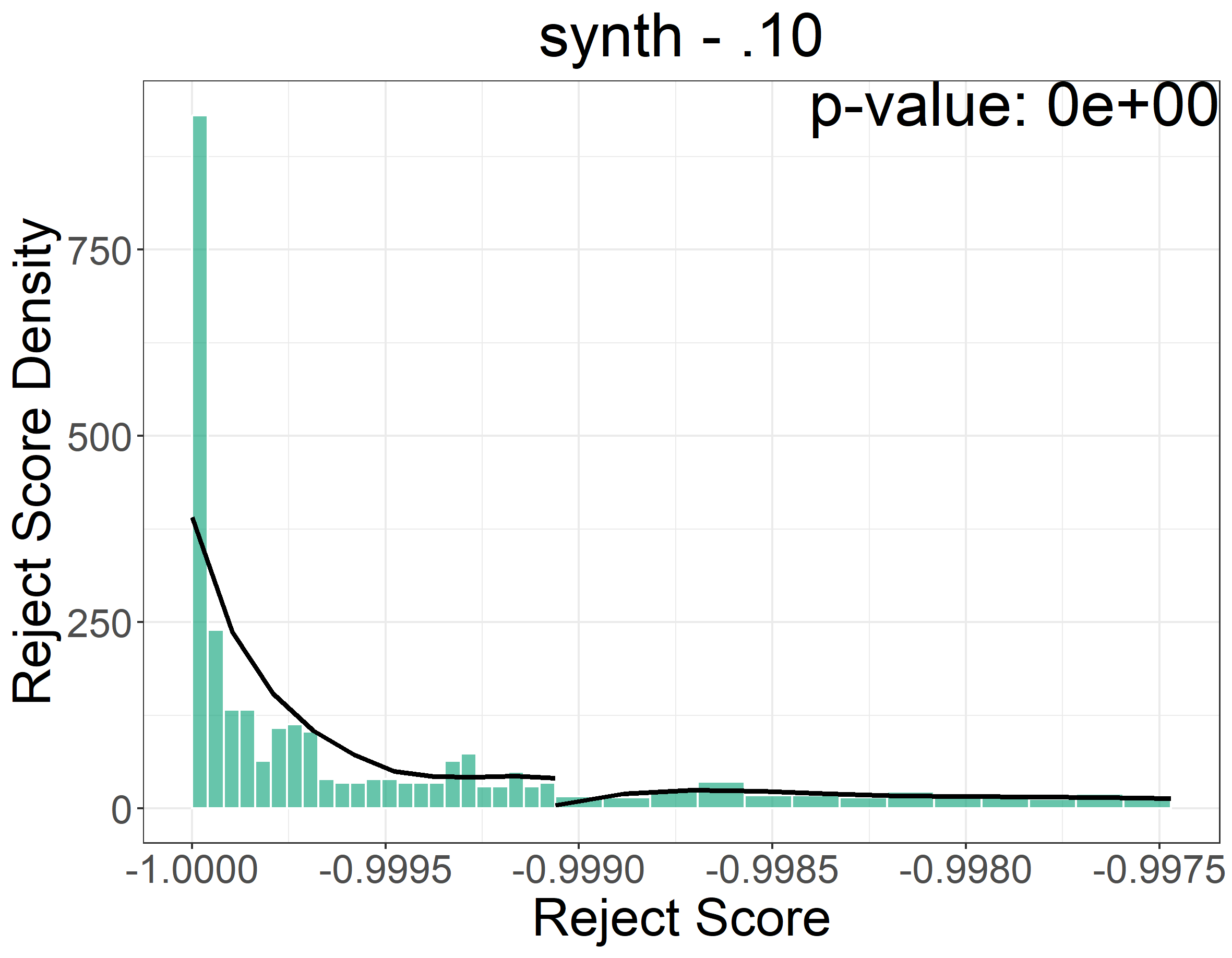
Refer to caption
(a) κ¯.10subscript¯𝜅.10\overline{\kappa}_{.10}.
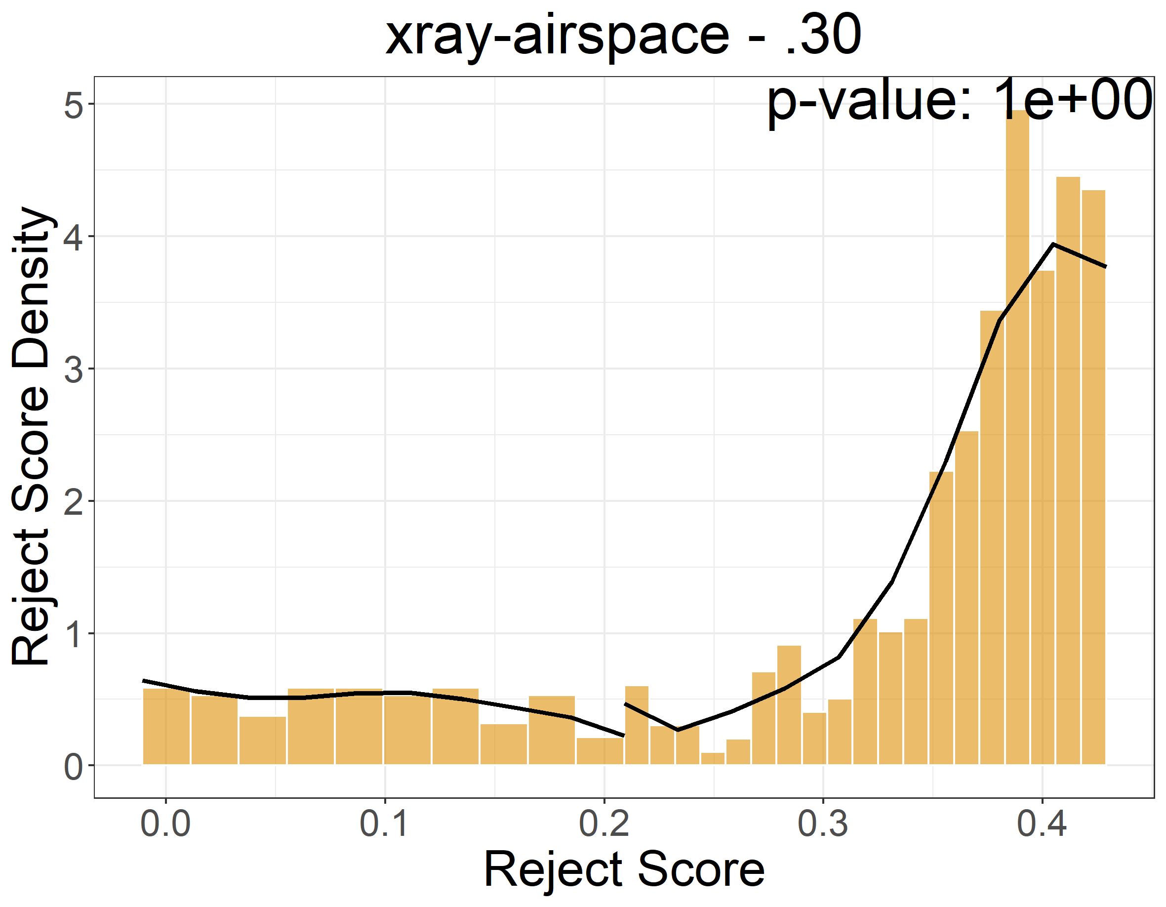
Refer to caption
(b) κ¯.20subscript¯𝜅.20\overline{\kappa}_{.20}.
Refer to caption
(c) κ¯.30subscript¯𝜅.30\overline{\kappa}_{.30}.
Refer to caption
(d) κ¯.40subscript¯𝜅.40\overline{\kappa}_{.40}.
Refer to caption
(e) κ¯.50subscript¯𝜅.50\overline{\kappa}_{.50}.
Refer to caption
(f) κ¯.60subscript¯𝜅.60\overline{\kappa}_{.60}.
Refer to caption
(g) κ¯.70subscript¯𝜅.70\overline{\kappa}_{.70}.
Refer to caption
(h) κ¯.80subscript¯𝜅.80\overline{\kappa}_{.80}.
Refer to caption
(i) κ¯.90subscript¯𝜅.90\overline{\kappa}_{.90}.
Figure 7: synth estimated best baseline (ASM) reject scores densities at the left and right of cutoff κ¯csubscript¯𝜅𝑐\overline{\kappa}_{c}. All the plots are zoomed around the cutoff values.
Refer to caption
(a) κ¯.10subscript¯𝜅.10\overline{\kappa}_{.10}.
Refer to caption
(b) κ¯.20subscript¯𝜅.20\overline{\kappa}_{.20}.
Refer to caption
(c) κ¯.30subscript¯𝜅.30\overline{\kappa}_{.30}.
Refer to caption
(d) κ¯.40subscript¯𝜅.40\overline{\kappa}_{.40}.
Refer to caption
(e) κ¯.50subscript¯𝜅.50\overline{\kappa}_{.50}.
Refer to caption
(f) κ¯.60subscript¯𝜅.60\overline{\kappa}_{.60}.
Refer to caption
(g) κ¯.70subscript¯𝜅.70\overline{\kappa}_{.70}.
Refer to caption
(h) κ¯.80subscript¯𝜅.80\overline{\kappa}_{.80}.
Refer to caption
(i) κ¯.90subscript¯𝜅.90\overline{\kappa}_{.90}.
Figure 8: cifar10h estimated best baseline (CC) reject scores densities at the left and right of cutoff κ¯csubscript¯𝜅𝑐\overline{\kappa}_{c}. All the plots are zoomed around the cutoff values.
Refer to caption
(a) κ¯.10subscript¯𝜅.10\overline{\kappa}_{.10}.
Refer to caption
(b) κ¯.20subscript¯𝜅.20\overline{\kappa}_{.20}.
Refer to caption
(c) κ¯.30subscript¯𝜅.30\overline{\kappa}_{.30}.
Refer to caption
(d) κ¯.40subscript¯𝜅.40\overline{\kappa}_{.40}.
Refer to caption
(e) κ¯.50subscript¯𝜅.50\overline{\kappa}_{.50}.
Refer to caption
(f) κ¯.60subscript¯𝜅.60\overline{\kappa}_{.60}.
Refer to caption
(g) κ¯.70subscript¯𝜅.70\overline{\kappa}_{.70}.
Refer to caption
(h) κ¯.80subscript¯𝜅.80\overline{\kappa}_{.80}.
Refer to caption
(i) κ¯.90subscript¯𝜅.90\overline{\kappa}_{.90}.
Figure 9: galaxyzoo estimated reject scores densities at the left and right of cutoff κ¯csubscript¯𝜅𝑐\overline{\kappa}_{c} for the best baseline CC. All the plots are zoomed around the cutoff values.
Refer to caption
(a) κ¯.10subscript¯𝜅.10\overline{\kappa}_{.10}.
Refer to caption
(b) κ¯.20subscript¯𝜅.20\overline{\kappa}_{.20}.
Refer to caption
(c) κ¯.30subscript¯𝜅.30\overline{\kappa}_{.30}.
Refer to caption
(d) κ¯.40subscript¯𝜅.40\overline{\kappa}_{.40}.
Refer to caption
(e) κ¯.50subscript¯𝜅.50\overline{\kappa}_{.50}.
Refer to caption
(f) κ¯.60subscript¯𝜅.60\overline{\kappa}_{.60}.
Refer to caption
(g) κ¯.70subscript¯𝜅.70\overline{\kappa}_{.70}.
Refer to caption
(h) κ¯.80subscript¯𝜅.80\overline{\kappa}_{.80}.
Refer to caption
(i) κ¯.90subscript¯𝜅.90\overline{\kappa}_{.90}.
Figure 10: hatespeech estimated best baseline (RS) reject scores densities at the left and right of cutoff κ¯csubscript¯𝜅𝑐\overline{\kappa}_{c}. All the plots are zoomed around the cutoff values.
Refer to caption
(a) κ¯.10subscript¯𝜅.10\overline{\kappa}_{.10}.
Refer to caption
(b) κ¯.20subscript¯𝜅.20\overline{\kappa}_{.20}.
Refer to caption
(c) κ¯.30subscript¯𝜅.30\overline{\kappa}_{.30}.
Refer to caption
(d) κ¯.40subscript¯𝜅.40\overline{\kappa}_{.40}.
Refer to caption
(e) κ¯.50subscript¯𝜅.50\overline{\kappa}_{.50}.
Refer to caption
(f) κ¯.60subscript¯𝜅.60\overline{\kappa}_{.60}.
Refer to caption
(g) κ¯.70subscript¯𝜅.70\overline{\kappa}_{.70}.
Refer to caption
(h) κ¯.80subscript¯𝜅.80\overline{\kappa}_{.80}.
Refer to caption
(i) κ¯.90subscript¯𝜅.90\overline{\kappa}_{.90}.
Figure 11: xray-airspace estimated best baseline (RS) reject scores densities at the left and right of cutoff κ¯csubscript¯𝜅𝑐\overline{\kappa}_{c}. All the plots are zoomed around the cutoff values.