Enhancing Security and Privacy in Federated Learning using Update Digests and Voting-Based Defense

Abstract

Federated Learning (FL) is a promising privacy-preserving machine learning paradigm that allows data owners to collaboratively train models while keeping their data localized. Despite its potential, FL faces challenges related to the trustworthiness of both clients and servers, especially in the presence of curious or malicious adversaries. In this paper, we introduce a novel framework named Federated Learning with Update Digest (FLUD), which addresses the critical issues of privacy preservation and resistance to Byzantine attacks within distributed learning environments. FLUD utilizes an innovative approach, the $\mathsf{LinfSample}$ method, allowing clients to compute the $l_{\infty}$ norm across sliding windows of updates as an update digest. This digest enables the server to calculate a shared distance matrix, significantly reducing the overhead associated with Secure Multi-Party Computation (SMPC) by three orders of magnitude while effectively distinguishing between benign and malicious updates. Additionally, FLUD integrates a privacy-preserving, voting-based defense mechanism that employs optimized SMPC protocols to minimize communication rounds. Our comprehensive experiments demonstrate FLUD’s effectiveness in countering Byzantine adversaries while incurring low communication and runtime overhead. FLUD offers a scalable framework for secure and reliable FL in distributed environments, facilitating its application in scenarios requiring robust data management and security.

I Introduction

I-A Background and Motivation

Federated Learning (FL) [1] is a distributed machine learning paradigm that enables data owners to collaboratively train models while keeping their data local, sharing only model updates with a central server. The server integrates these updates based on an Aggregating Rule (AR), thus facilitating collaborative model training. Notably, models trained via FL can achieve accuracies comparable to those trained with centralized methods [2].

However, the effectiveness of FL crtically depends on the trustworthiness of both the data owners (i.e., clients) and the server. The presence of curious or malicious adversaries in FL introduces a complex interplay between clients and servers [3, 4, 5, 6]. In classic AR such as Federated Averaging (FedAvg) [1], the server performs the weighted averaging-based aggregation on updates from clients indiscriminately. This process is vulnerable to Byzantine adversaries that may tamper with local data or modify the training process to generate poisoned local model updates [7]. Studies [8, 9, 10] have demonstrated that even a single malicious client can cause the global model derived from FedAvg to deviate from the intended training direction. Byzantine adversaries may also execute attacks sporadically [10, 11], including backdoor attacks that may require only a single round to embed a persistent backdoor in the global model [8, 9]. Since the server cannot access the client’s data, Byzantine-resistant aggregation rule (BRAR) [10, 12, 5, 13] needs to be implemented.

Moreover, the server may compromise clients’ data privacy, e.g., through data reconstruction attacks [14, 15, 16] or source attacks [17] simply by analyzing the plaintext updates from clients. For example, DLG [14] initially generates a random input $X^{\prime}$ and then calculates the $l_{2}$ distance between the fake gradient and the real plaintext gradient as the loss function. InvertGrad [16] employs cosine distance and total variation as the loss function. As such, clients need to encrypt or perturb the uploaded updates. However, considering the false sense of security [18] brought by perturbation and quantization, mechanisms such as Secure Multi-Party Computation (SMPC) [19, 20] are necessary to safeguard the privacy of updates.

I-B Related Work

In scenarios with limited prior knowledge, such as the number of malicious clients (assumed to be $\beta$), the server is required to compute statistical information of updates, including geometric distance, median, and norm. The Multikrum [10] selects multiple updates that have the smallest sum of distances to the other $m-\beta-2$ nearest updates, where $m$ is number of clients. Trimmedmean [12] sorts the values of each dimension of all updates and then removes the $\beta$ extreme values in that dimension, calculating the average of the remaining values as the global update for that dimension. However, these methods of dimensional level and distance calculation have been proven to be very vulnerable under complex attacks [7, 21].

In the absence of prior knowledge, the server uses clustering, clipping, and other methods to limit the impact of poisoned updates on the global model from multiple aspects. ClippedClustering [22] adaptively clips all updates using the median of historical norms and uses agglomerative hierarchical clustering to divide all updates into two clusters, averaging all updates in the larger cluster. DNC [7] uses singular value decomposition to detect and remove outliers and randomly samples its input updates to reduce dimensions. MESAS [23] carefully selects six metrics about the local model that can maximally filter malicious models.

Trust-based methods assume that the server collects a clean small root dataset to bootstrap trust or assumes that clients will honestly propagate on the local model with a specified dataset. In FLTrust [5] and FLOD [6], the server uses a clean dataset to defend against a large fraction of malicious clients. Updates with directions greater than 90 degrees are discarded, and the remaining updates are aligned with the clean updates in norm and aggregated according to cosine similarity. However, FLOD [6] uses signed updates for aggregation, which increases the number of rounds required for convergence and decreases the accuracy of the global model. FLARE [24] requires users to perform forward propagation on a specified dataset and upload penultimate layer representations, calculating the maximum mean discrepancy of these representations as the distance between models. Those updates that are selected as neighbors the most times.

The cost of converting very complex BRAR into privacy-preserving computation protocols is significant, and not less than performing secure inference on a model with input length in the millions. Therefore, privacy-preserving BRAR (ppBRAR) cannot use complex statistical metrics to ensure its practicality. PPBR [25] designs a 3PC-based maliciously secure top-$k$ protocol to calculate the sum of the largest $k$ similarities for each update as a score, and selects the updates with the highest scores for weighted average aggregation. shieldFL [3], based on double-trapdoor HE, calculates the cosine similarity between each local update and the global update of the previous round, considering the lowest similarity as malicious and assigning lower weights to updates close to it. However, it assumes that all local updates in the first round are benign, which is unrealistic when the adversary is static from the start. Specifically, LFR-PPFL [26] tracks the change in distance between pairwise updates to find malicious clients, but this includes an assumption of a static adversary, i.e., malicious clients engage in malicious behavior every round. RoFL [27] and ELSA [28] limit the norm of all updates to mitigate the destructiveness of poisoned updates, the former using zero-knowledge proofs to ensure the correctness of the norm, the latter using multi-bit Boolean secret sharing to ensure the norm bound. However, when the number of corrupted clients increases, the accuracy of the global model will decrease significantly.

Methods that simultaneously address the plaintext leakage of updates and the problem of Byzantine adversary transform BRAR into ppBRAR [4, 6, 3] via SMPC. This approach involves replacing a centralized server with multiple distributed servers. As a result, traditional aggregation protocols are converted into SMPC protocols. Consequently, model updates are transmitted to these servers either as ciphertext or as shares, which then serve as inputs for the computation protocols. Acting as computing parties, these servers collaboratively execute the ppBRAR protocol. However, the SMPC overhead for deploying trained detection models on servers or implementing methods like PCA is often prohibitive.

Consequently, many ppBRARs adopt heuristic methods and utilize relatively simple statistical features to distinguish between malicious and benign clients, such as sign [29], geometric distance [10], cosine similarity [25], $l_{2}$ norm [28, 27], and clustering methods [4]. In the absence of prior knowledge, such as a clean dataset, ppBRARs often need to perform statistical measurements on all entries of the updates. For the SMPC overhead of pairwise distances/similarities between $m$ $d$-dimensional updates, it introduces $\binom{m}{2}$ times $d$-dimensional Hadamard products [6, 25, 4], thereby accounting for more than 80% of the duration of the entire scheme [4]. Therefore, reducing the computational overhead of pairwise distance calculations has become an urgent task to be addressed.

I-C Contributions of this Paper

Considering the above issues, we first simulate 8 advanced attacks with a 40% malicious client ratio. We observe that malicious updates from straightforward attacks can be filtered out based solely on a global $l_{\infty}$ norm. For those poisoned updates that inject subtle deviations based on the mean and variance of all benign updates or are trained on tampered samples, we find that using sliding windows to calculate the $l_{\infty}$ vector of model updates can still capture the subtle differences between them and benign updates. Therefore, we suggest using update digests to calculate the shared distance matrix instead of the model updates themselves, which can significantly reduce the computational overhead related to SMPC on servers. Moreover, we introduce a novel privacy-preserving voting filter strategy aimed at eliminating poisoned updates. This strategy involves converting the sharing of the distance matrix into the sharing of the voting matrix, achieved by parallel computing the median of all rows of the matrix. The contributions of this paper are summarized as follows:

• We propose FLUD, which includes an update digest calculation method termed $\mathsf{LinfSample}$, a privacy-preserving voting-based defense method that can filter out poisoned model updates. $\mathsf{LinfSample}$ employs a sliding window to gather $l_{\infty}$ on updates, where clients are only required to bear the additional computation and upload the sharing of update digest. Meanwhile, the server experiences a reduction in the computational overhead for the distance matrix by three orders of magnitude, thereby enhancing the security and privacy of Federated Learning in a streamlined manner.

• We further design carefully optimized privacy-preserving SMPC protocols for FLUD, including packed comparison techniques for arithmetic shares, Additive Homomorphic Encryption (AHE)-based multi-row shuffle protocols, and quick select protocols based on packed comparison. These protocols adopt parallel techniques and significantly reduce the number of communication rounds, enhancing the efficiency and scalability of our system.

• Through extensive comparative experiments, we demonstrate the robustness of the $\mathsf{LinfSample}$ method and FLUD against Byzantine adversaries. We also assess the communication and runtime overhead of the designed SMPC protocols across a spectrum of models and client populations. The results affirm FLUD’s strong Byzantine resistance and extremely low communication and runtime overhead.

II Preliminaries

II-A Federated Learning

A classical FL algorithm typically includes an initial step 1, followed by $T$ repetitions of steps 2-4.

• Step 1: The server initializes a global model randomly.

• Step 2: At the global round $t$, the server selects a set of clients $\mathcal{C}_{t}$ and broadcasts the global model $\boldsymbol{\omega}^{t}$.

• Step 3: Each client $i$ locally performs the replacement $\boldsymbol{\omega}_{i}^{t}\leftarrow\boldsymbol{\omega}^{t}$ and estimates the gradients of the loss function over their private dataset for $E$ epochs. Then $i$ computes and uploads the local model update $\boldsymbol{g}_{i}^{t}\leftarrow\boldsymbol{\omega}_{i}^{t}-\boldsymbol{\omega}^{t}$.

• Step 4: The server collects the local model updates and utilizes an AR to compute the global update, which is then used to update the global model.

Note that when the aggregating party implements ppBRAR, the centralized server is replaced by multiple distributed servers.

II-B Byzantine Attacks in FL

The Byzantine adversary encompasses a spectrum of malicious behaviors, whereby compromised clients manipulate local data or the training process to generate poisoned updates, in an attempt to disrupt the training process of the global model. Specifically, these attacks can be classified into Untargeted and Targeted attacks based on their objectives. We denote the set of clients corrupted by the adversary as $\mathcal{C^{\prime}}$.

II-B1 Untargeted attacks

In untargeted attacks, adversaries construct malicious updates that, when aggregated, cause the model to lose usability or extend the number of rounds required for convergence. The types of attacks that can be implemented vary depending on the knowledge and capabilities possessed by the adversary.

Adversaries with limited knowledge and capabilities only know the local data and training process of the compromised clients. The attacks they can launch include:

• LabelFlipping [11]. The adversary flips the labels of all local samples. For example, in a dataset with $10$ classes, the label of all samples is set to $9-y$, where $y$ is the actual label.

• SignFlipping [30]. After the adversary calculates the gradient each time, it flips the signs of all the entries, and then uses it to update the local model. This is essentially a reversed gradient descent method.

• Noise-$(\mu,\sigma^{2})$ [30]. The adversary uploads a vector $\boldsymbol{x}$, each element of which follows $\mathcal{N}(\mu,\sigma^{2})$. Here we set the sampling source to be the standard normal distribution, denoted as Noise-(0,1).

The adversary, knowing all the model updates from benign clients, skillfully constructs the following attack by calculating the mean ($\mu_{j}$) and variance ($\sigma_{j}$) for each dimension $j$:

• ALIE [31]. The adversary uses the Inverse Cumulative Distribution Function (ICDF) of a standard normal distribution to calculate $\alpha$, representing an upper limit of the standard normal random variable. For each $i\in\mathcal{C^{\prime}}$, $\boldsymbol{g}_{i,j}=\mu_{j}+\sigma_{j}\cdot\alpha$, creating a certain offset in the generated updates.

• MinMax [32]. The adversary computes a scaling factor $\alpha$ to ensure that the maximum distance from the malicious update $\boldsymbol{g}{i}$ to any benign update does not exceed the maximum distance between any two benign updates. Each component of the malicious update, $\boldsymbol{g}_{i,j}$, is calculated as $\mu_{j}+\sigma_{j}\cdot\alpha$.

• IPM-$\alpha$ [33]. The adversary directs all the corrupted clients upload an average update in the opposite direction, scaled by $\alpha$. Specifically, for every client $i$ in $\mathcal{C^{\prime}}$, $\boldsymbol{g}_{i}=-\frac{\alpha}{|\mathcal{C}\setminus\mathcal{C^{\prime}}|}\sum_{j\in\mathcal{C}\setminus\mathcal{C^{\prime}}}\boldsymbol{g}_{j}$. Here we set two values for $\alpha$, 0.1 and 100, as two types of attacks, denoted as IPM-0.1 and IPM-100, respectively.

II-B2 Targeted attack / Backdoor attack[8, 9]

The adversary embeds a trigger, such as a visible white square or a subtle perturbation, into features and changes their labels to a specific target. The poisoned model predicts correctly on clean samples, but it predicts samples with triggers as the target label. In practice, we let the adversary manipulates all corrupted clients by placing a $6\times 6$ pixel white block in the top-left corner of half of their samples and setting the target label to 0.

Therefore, we simulate the following eight types of attacks: LabelFlipping, SignFlipping, Noise-(0,1), ALIE, MinMax, IPM-0.1, IPM-100, and Backdoor. At the beginning of FL, the adversary will control all clients in $\mathcal{C}^{\prime}$ to launch one of these attacks.

II-C Additive Secret Sharing

Additive secret sharing [19] is a commonly used two-party computation (2PC) technique that allows two computing parties, $S_{0}$ and $S_{1}$, to perform efficient linear computations on shares. It is frequently combined with oblivious transfer, garbled circuits, and homomorphic encryption to create hybrid protocols. The commonly used building blocks for additive secret sharing operate as follows:

$\mathsf{Split}(x)\rightarrow\langle x\rangle$: The holder of the secret $x\in\mathbb{Z}_{2^{l}}$ selects a random number $r\overset{\$}{\leftarrow}\{0,1\}^{l}$ as $\langle x\rangle_{0}$ and computes the $\langle x\rangle_{1}=x-r\mod 2^{l}$. Then $\langle x\rangle_{b}$ are to $S_{b}$, $b\in\{0,1\}$. $\langle x\rangle$ is considered as the Arithmetic sharing of $x$. Here we adopt a more practical approach, where the holder and $S_{0}$ use a pre-negotiated seed to generate $\langle x\rangle_{0}$, thereby reducing communication overhead by half.

$\mathsf{Reavel}(\langle x\rangle)\rightarrow x$: Party $S_{b}$ sends $\langle x\rangle_{b}$ to $S_{b-1}$. Subsequently, $S_{b}$ locally computes $x=\langle x\rangle_{0}+\langle x\rangle_{1}\mod 2^{l}$ to recover $x$.

$\mathsf{ADD}(\langle x\rangle,\langle y\rangle)\rightarrow\langle z\rangle$: To compute the sum $\langle z\rangle=\langle x+y\rangle$, $S_{b}$ locally computes $\langle z\rangle_{b}=\langle x\rangle_{b}+\langle y\rangle_{b}\mod 2^{l}$.

$\mathsf{MUL}(\langle x\rangle,\langle y\rangle)\rightarrow\langle z\rangle$: For computing the product $\langle z\rangle=\langle x\cdot y\rangle$, $S_{0}$ and $S_{1}$ utilize pre-generated Beaver triples $\langle a\rangle$, $\langle b\rangle$, $\langle c\rangle$, where $c=a\cdot b$. $S_{0}$ and $S_{1}$ recover $e=x-a$ and $f=y-b$. Then, $S_{0}$ computes locally $\langle z\rangle_{0}=ef+e\langle b\rangle_{0}+f\langle a\rangle_{0}+\langle c\rangle_{0}\mod 2^{l}$, while $S_{1}$ computes locally $\langle z\rangle_{1}=e\langle b\rangle_{1}+f\langle a\rangle_{1}+\langle c\rangle_{1}\mod 2^{l}$.

In particular, when $l=1$, we denote the sharing of $x\in\{0,1\}$ as Boolean sharing $\langle x\rangle^{B}$. In this case, we substitute $\mathsf{XOR}$ and $\mathsf{AND}$ for $\mathsf{ADD}$ and $\mathsf{MUL}$, respectively. Additionally, a function exists that converts Boolean sharing to Arithmetic sharing: $\mathsf{B2A}(\langle x\rangle^{B})\rightarrow\langle z\rangle$. For further details, please refer to [20].

II-D Additive Homomorphic Encryption

AHE allows operations on ciphertexts which correspond to addition or multiplication in the plaintext space, without the need to decrypt. The plaintext space for AHE is $M$, and the ciphertext space is $C$. AHE consists of three functions and two operations:

$\mathsf{KeyGen}(1^{\kappa})\rightarrow(sk,pk)$: Given a security parameter $\kappa$, generate a key pair, where $pk$ is used for encryption, and $sk$ for decryption.

$\mathsf{Enc}(m,pk)\rightarrow c$: Anyone with the public key $pk$ can encrypt a plaintext $m$ to a ciphertext $c$.

$\mathsf{Dec}(c,sk)\rightarrow m$: Only the person with the private key $sk$ can decrypt a ciphertext $c$ to get a plaintext $m$.

$\oplus$, $\boxplus$: Furthermore, for any plaintexts $m_{1},m_{2}\in M$, it holds that $\mathsf{Dec}(\mathsf{Enc}(m_{1})\oplus\mathsf{Enc}(m_{2}))=m_{1}+m_{2}$ and $\mathsf{Dec}(\mathsf{Enc}(m_{1})\boxplus m_{2})=m_{1}+m_{2}$. Hence, performing the $\oplus$ or $\boxplus$ operation on ciphertexts is equivalent to performing addition in the plaintext space.

The AHE scheme used in this paper is the Paillier [34], with the length of the plaintext space $M$ being 1024 bits and the length of the ciphertext space $C$ being 2048 bits.

III Overview

III-A System Model

The system model (Fig. 1) includes two components:

Client Side: This side consists of $m$ clients, with each client $i$ possessing a local dataset $\mathcal{D}_{i}$. During each global iteration in FL, client $i$ computes update using $\mathcal{D}_{i}$ based on the latest global model. If client $i$ is corrupted by the byzantine adversary, it will construct a poisoned model update according to the type of attack. It also generates an update digest, and uploads both the update and the digest in the form of sharing to the servers.

Aggregator Side: This side involves two servers responsible for performing aggregations. After receiving the shares in each global round, they execute a secure aggregation process involving a series of 2PC protocols to filter the poisoned updates and compute the new global model. The 2PC protocols involve computing the sharing of the Squared Euclidean Distance (SED) matrix, the medians of the rows, the voting matrix and the new global update.

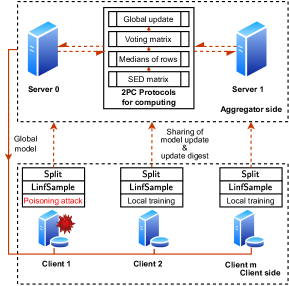
Figure 1: System model

III-B Threat Model

We consider a Byzantine adversary $\mathcal{A}_{f}$ that can corrupt fewer than half of the clients. This setting is consistent with previous works [21, 4, 25, 35]. It controls the set of corrupted clients $\mathcal{C}^{\prime}$ to implement any one of 8 types of attacks described in Sec. II-B.

Moreover, we consider a static probabilistic polynomial time adversary, $\mathcal{A}_{h}$, who is also honest-but-curious [36, 20]. It could control at most one of the servers $S_{0}$ and $S_{1}$ at the beginning of FLUD. $\mathcal{A}_{h}$ will faithfully execute the designed 2PC protocols but will also attempt to infer private information about clients from the sharing and from the transcripts of the 2PC protocols. We define the security of the 2PC protocols using the same simulation paradigm [20]. For example, consider a 2PC protocol $\Pi$ that encompasses multiple sub-protocols $\{A,\ldots,Z\}$. We replace the real-world implementation of $\Pi$ with the corresponding ideal functionalities $\{\mathcal{F}_{A},\ldots,\mathcal{F}_{Z}\}$ for these sub-protocols, thereby constructing the $(\mathcal{F}_{A},\ldots,\mathcal{F}_{Z})$-hybrid model. $\Pi$ is considered secure if, within the $(\mathcal{F}_{A},\ldots,\mathcal{F}_{Z})$-hybrid model, the simulator $\mathcal{S}$ cannot distinguish the protocol’s behavior in the real world from its behavior in the ideal world.

III-C Design Goals

Byzantine Robustness. With the distance matrix computed based on update digests and the implementation of the voting method, their combination empowers FLUD to defend against each of the eight attacks listed in Sec. II-B.

Privacy Preservation. The secure aggregation process does not leak any statistical information about updates, and servers cannot learn anything more than which clients’ updates will be aggregated.

Efficiency. FLUD has to incur lower overhead in the 2PC protocols as compared to existing schemes which compute distances and clustering [35, 22] on full-sized updates.

Scalability. Our designed 2PC protocols have excellent communication round complexity and runtime overhead, enabling FLUD to scale effectively with an increasing number of clients.

IV Defense idea

IV-A Observation

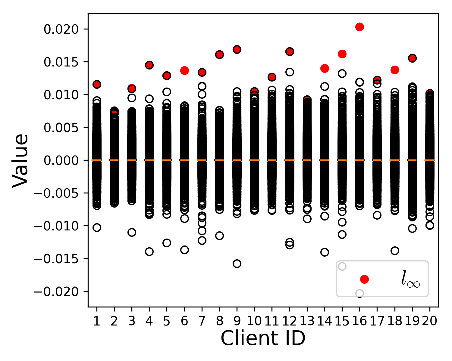
(a) LabelFlipping

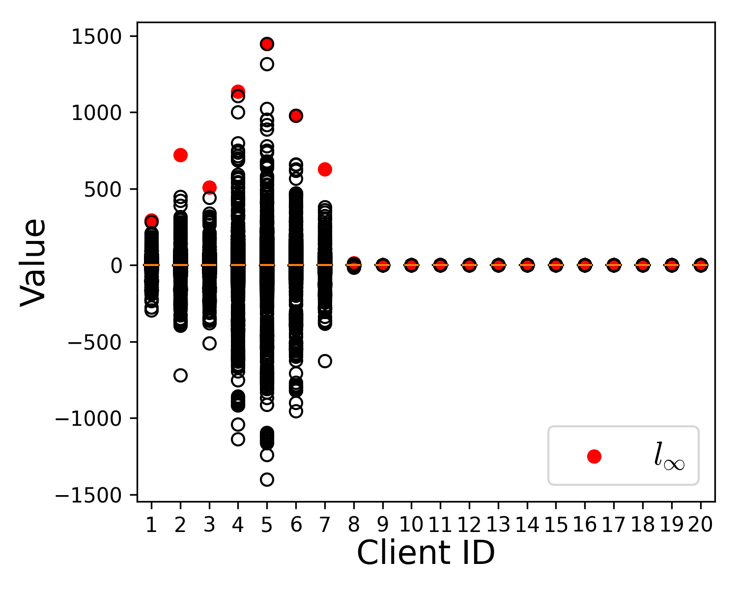
(b) SignFlipping

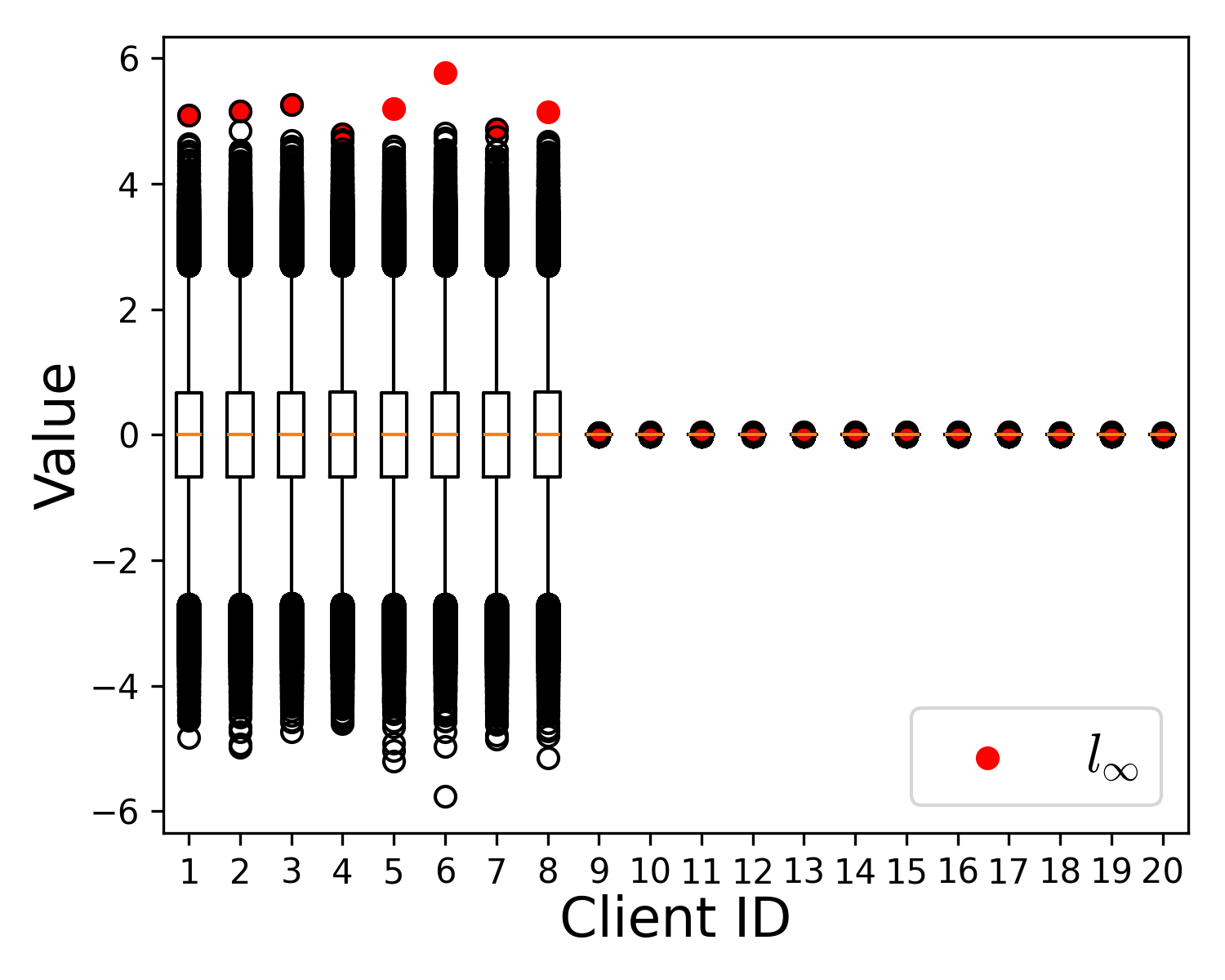
(c) Noise-(0,1)

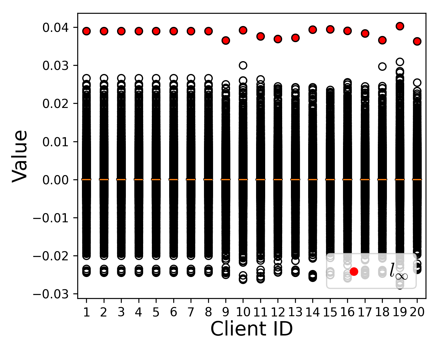
(d) ALIE

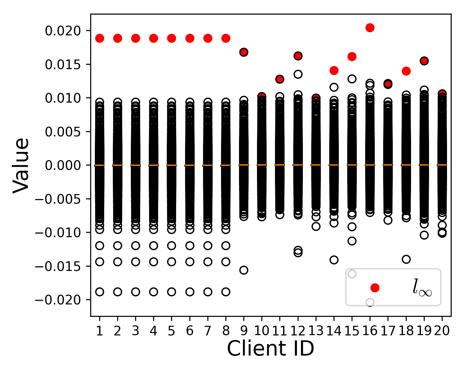
(e) MinMax

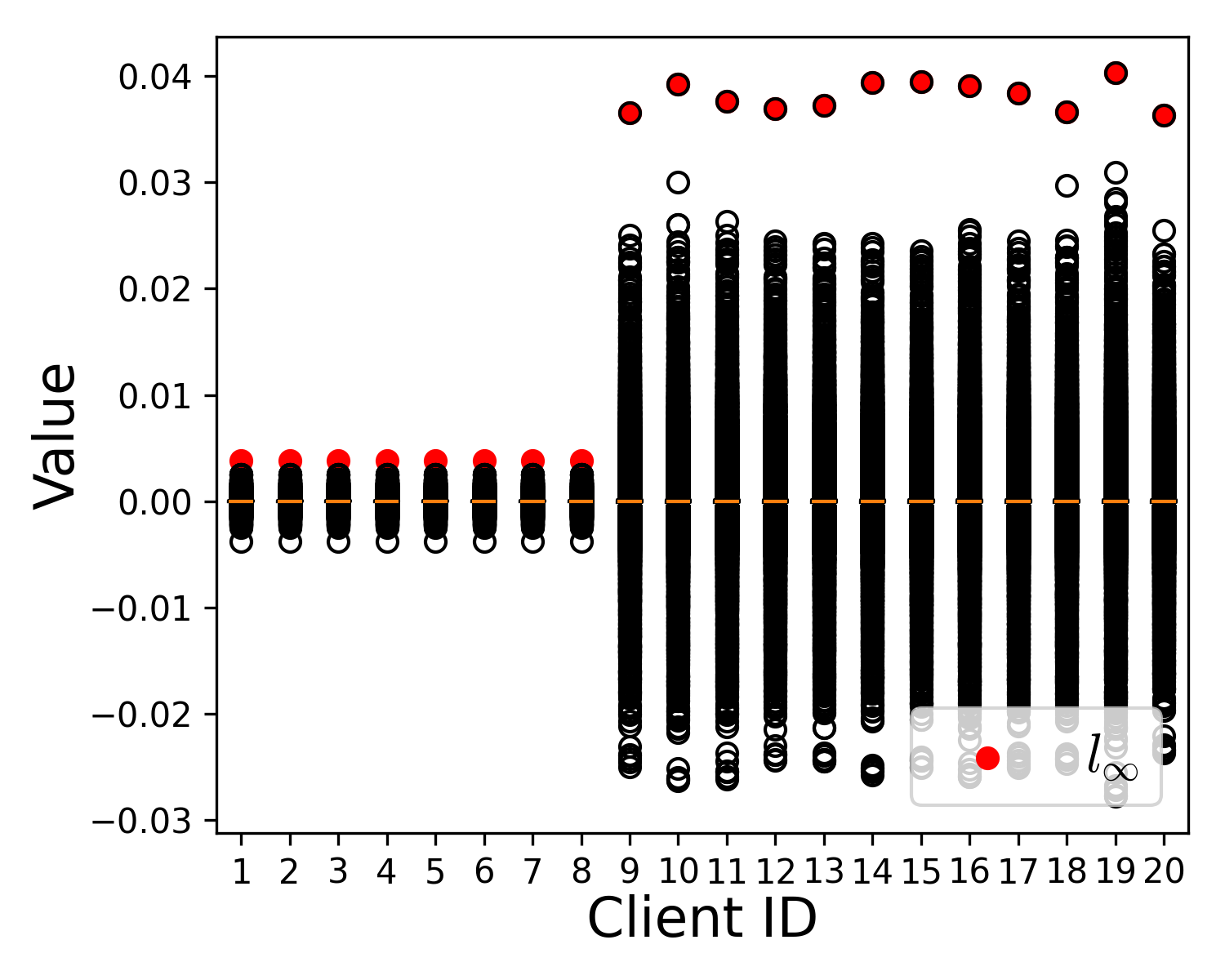
(f) IPM-0.1

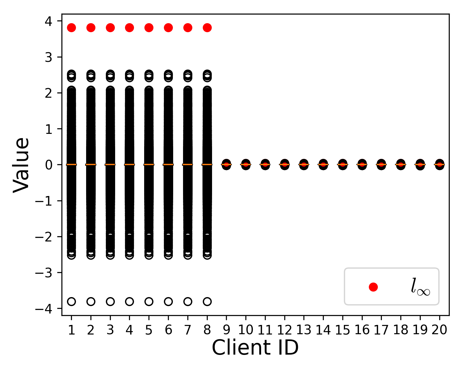
(g) IPM-100

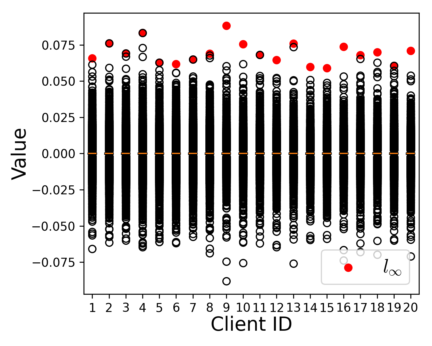
(h) Backdoor

Figure 2: Box plots of model updates from 20 clients and their global $l_{\infty}$ norms, where clients with IDs 1-8 are malicious clients executing specific attacks, and clients with IDs 9-20 are benign clients.

We plot box plots of the updates constructed via $8$ attacks mentioned in Sec. II-B in Fig.2. The dataset is CIFAR-10, and the setting for the ResNet10 model is consistent with Sec. VI-A. Clients 1-8 are controlled by Byzantine adversary, and clients 9-20 are benign clients. We observe that Byzantine attacks can be categorized into three types.

The first type comprises amplified updates, where the absolute values in most dimensions are greater than those in benign updates. Aggregating such updates would result in a significant shift in the global model towards the incorrect direction, leading to a loss of usability. It includes SignFlipping, Noise-(0,1) and IPM-100. The second type consists of diminished updates, where the amplitudes in most dimensions are smaller than those in benign updates. Aggregating such updates would slow down the global model or reduce its final convergence accuracy. It includes IPM-0.1. Both of the above types are easily detectable by distance detection algorithms since the global $l_{\infty}$ norm of these poisoned updates represents an extremum. For ease of exposition, we refer to the first type of updates as Up-scaled Updates and the second type as Down-scaled Updates.

The third type consists of meticulously crafted updates, which are fine-tuned based on the mean and variance of benign updates, or updates trained from poisoned data. We refer to this type of updates as Mix-scaled Updates. It includes LabelFlipping, ALIE, MinMax and Backdoor. The norm or global $l_{\infty}$ of these updates is typically similar to that of benign updates. Next, we flatten all updates and sample them using a sliding window of size $4096$ to compute the vectors of $l_{\infty}$ norms. We then calculate the pairwise SEDs between vectors and represent them in the form heatmaps in Fig.3. It is evident that this sampling method still effectively discerns between poisoned and benign updates.

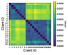
(a) LabelFlipping

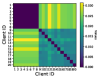
(b) ALIE

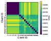
(c) MinMax

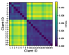
(d) Backdoor

Figure 3: Pairwise SEDs between 20 update digests. Here, clients utilize a sliding window to capture the $l_{\infty}$ norms of their local model updates and then concatenate all the $l_{\infty}$ values into a new vector termed the update digest.

From the observations above, we can infer that each sliding window of updates exhibits similarity in its positive and negative fluctuation ranges. We summarize the schematics of benign updates and the three types of poisoned updates in Fig. 4. The $l_{\infty}$ norms in each sliding window of benign updates remain similar, whereas those in poisoned updates exhibit significant deviations. Mix-scaled updates, however, may display variations in $l_{\infty}$ norms, with some being smaller and others larger than those observed in benign updates. Therefore, mix-scaled updates still show variations in $l_{\infty}$ norms as compared to benign updates. By using sliding window analysis, servers not only pinpoint these discrepancies but also also benefit from a significant reduction in the computational overhead required for shared pairwise distance calculations compared to analyses based on the full-size updates.

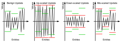
Figure 4: A schematic representation of benign updates and three types of poisoned updates.

IV-B Filtering Method

Since Byzantine adversaries operate covertly and can launch attacks in any round, we need to compute pairwise distances in each round.

IV-B1 Linfsample

The $\mathsf{LinfSample}$ consists of two steps for client $i$: 1. Flatten the entire model update: $\boldsymbol{f}_{i}\leftarrow\mathsf{flatten}(\boldsymbol{g}_{i})$. 2. Compute the $l_{\infty}$ of entries selected by the sliding window as Eq. 1:

$$\boldsymbol{d}_{i,j}=\max\left\{\lvert\boldsymbol{f}_{i,s\cdot i+k}\rvert\;\middle|\;k=0,1,...,s-1\right\},\quad j=1,2,...,l^{\prime}$$ (1)

where the window size and stride are both set to $s$ with the ceiling mode. The value of $s$ is discussed in Sec. VI-D. Assuming the length of $\boldsymbol{f}_{i}$ is $l$, the length of the update digest is given by $l^{\prime}=\lfloor\frac{l}{s}\rfloor+1\{s\,|\,l\}$.

IV-B2 Mutual Voting

Since our threat model assumes that the majority of clients are honest, without prior knowledge and clean datasets, a common approach is to find a cluster comprising more than half of the total updates. As updates are unlabeled, traditional KNN clustering cannot be used. Therefore, we design a voting mechanism similar to an unlabeled KNN. Assuming there are $m$ participating clients, each client can vote for the $m$ closest clients (including itself). Then, clients receiving at least $\frac{m}{2}$ votes are deemed benign, and their updates are aggregated by weighted averaging to form the global update.

V Construction

V-A Framework

We propose the FLUD framework (Alg. 1) designed to enhance model robustness against adversarial manipulations by employing a 2PC based ppBRAR. The framework operates with servers $S_{0}$ and $S_{1}$, $m$ clients, their local datasets and public preset parameters.

On the client side, after local training, each client applies the $\mathsf{LinfSample}$ technique, as described in Sec. IV-B1, to their update $\boldsymbol{g}_{i}$, obtaining the update digest $\boldsymbol{d}_{i}$. This update digest and model update are then shared with the servers via the practical $\mathsf{Split}$, as described in Sec. II-C.

On the aggregator side, servers compute the shared SED matrix $\langle\boldsymbol{M}\rangle$ of $m$ digests. Assume that the length of $\boldsymbol{d}_{i}$ is $k$. Specifically, for $i,j\in[1,m]$ where $i\neq j$, they compute $\langle\boldsymbol{tmp}\rangle\leftarrow\mathsf{MUL}(\langle\boldsymbol{d}_{i}\rangle-\langle\boldsymbol{d}_{j}\rangle,\langle\boldsymbol{d}_{i}\rangle-\langle\boldsymbol{d}_{j}\rangle)$ and set $\langle\boldsymbol{M}_{i,j}\rangle\leftarrow\mathsf{ADD}(\langle\boldsymbol{tmp}_{1}\rangle,\ldots,\langle\boldsymbol{tmp}_{k}\rangle)$. For cases where $i=j$, servers set $\langle\boldsymbol{M}_{i,j}\rangle_{0}=\langle\boldsymbol{M}_{i,j}\rangle_{1}=0$.

Algorithm 1 The FLUD framework

1:Input: Client set $\mathcal{P}=\{P_{1},P_{2},\ldots,P_{m}\}$, two servers $S_{0}$ and $S_{1}$, the number of global rounds $T$, local learning rate $\eta_{l}$, batch size $b$, the collection of local datasets $\mathcal{D}=\{\mathcal{D}_{1},\mathcal{D}_{2},\ldots,\mathcal{D}_{m}\}$, the size $s$ of the sampling window used by $\mathsf{LinfSample}$

2:Output: Global model parameter $\boldsymbol{\omega}$

3:Randomly initialize the global model $\boldsymbol{\omega}_{0}$

4:for global round $t\in[0,T-1]$ do

5:     $\triangleright$ Client side:

6:     for each client $i\in[1,m]$ in parallel do

7:         Run $\text{SGD}(b,\boldsymbol{\omega}_{t},\mathcal{D}_{i},\eta_{l})$ for $E$ epochs to get $\boldsymbol{g}_{i}$

8:         $\boldsymbol{d}_{i}\leftarrow\mathsf{LinfSample}(\boldsymbol{g}_{i},s)$

9:         $\mathsf{Split}(\boldsymbol{d}_{i})\rightarrow\langle\boldsymbol{d}_{i}\rangle$, $\mathsf{Split}(\boldsymbol{g}_{i})\rightarrow\langle\boldsymbol{g}_{i}\rangle$

10:     end for

11:     $\triangleright$ Aggregator side:

12:     Calculate the shared SED matrix $\langle\boldsymbol{M}\rangle$ of $\{\langle\boldsymbol{d}_{i}\rangle\}_{i\in[1,m]}$

13:     // Compute the shared voting matrix of $\{\langle\boldsymbol{d}_{i}\rangle\}_{i\in[1,m]}$

14:     $\langle\tilde{\boldsymbol{M}}\rangle\leftarrow\mathsf{matrixSharedShuffle}(\langle\boldsymbol{M}\rangle)$

15:     $\langle\mu_{1}\rangle,\ldots,\langle\mu_{m}\rangle\leftarrow\mathsf{mulRowQuickSelect}(\langle\tilde{\boldsymbol{M}}\rangle,\frac{m}{2}*m)$

16:     Reshape $\{\langle\mu_{1}\rangle*m,\ldots,\langle\mu_{m}\rangle*m\}$ into an $m\times m$ matrix $\langle\mathcal{U}\rangle$

17:     $\langle r_{1}\rangle^{B},\ldots,\langle r_{m^{2}}\rangle^{B}\leftarrow\mathsf{packedCompare}(\mathsf{flt}(\langle\boldsymbol{M}\rangle),\mathsf{flt}(\langle\mathcal{U}\rangle))$

18:     $\langle r_{1}\rangle,\ldots,\langle r_{m^{2}}\rangle\leftarrow\mathsf{B2A}(\langle r_{1}\rangle^{B},\ldots,\langle r_{m^{2}}\rangle^{B})$

19:     Reshape $\{\langle r_{1}\rangle,\ldots,\langle r_{m^{2}}\rangle\}$ into an $m\times m$ shared voting matrix $\langle\boldsymbol{V}\rangle$

20:     // Calculate the number of votes each client $i$ received

21:     For $i\in[1,m]$, $\langle v_{i}\rangle\leftarrow\mathsf{ADD}(\{\langle\boldsymbol{V}_{1,i}\rangle,\ldots,\langle\boldsymbol{V}_{m,i}\rangle\})$

22:     // Find clients that received at least $\frac{m}{2}$ votes

23:     $\langle e_{1}\rangle^{B},\ldots,\langle e_{m}\rangle^{B}\leftarrow\mathsf{packedCompare}((\frac{m}{2}-1)*m,\{\langle v_{i}\rangle\}_{i\in[1,m]})$

24:     $e_{1},\ldots,e_{m}\leftarrow\mathsf{Reveal}(\langle e_{1}\rangle^{B},\ldots,\langle e_{m}\rangle^{B})$

25:     Collect those indices $i$ whose $e_{i}=1$ into $\mathcal{Y}$

26:     $\langle\boldsymbol{g}\rangle\leftarrow\mathsf{ADD}(\{\mathsf{MUL}(\frac{|\mathcal{D}_{i}|}{\sum_{i}{|\mathcal{D}_{i}|}}\cdot\langle\boldsymbol{g}_{i}\rangle)\}_{i\in\mathcal{Y}})$

27:     $\boldsymbol{g}\leftarrow\mathsf{reveal}(\langle\boldsymbol{g}\rangle)$

28:     Broadcast $\boldsymbol{\omega}\leftarrow\boldsymbol{\omega}-\boldsymbol{g}$ to $\mathcal{P}$

29:end for

30:return $\boldsymbol{\omega}$

The operations performed in lines 11-17 transform the shared SED matrix into the shared voting matrix. To prevent the leakage of distance relationships among clients due to the revelation of comparison results during the subsequent quick select process [4, 37], servers invoke $\mathsf{matrixSharedShuffle}$ to independently shuffle all rows of $\langle\boldsymbol{M}\rangle$ and produce $\langle\tilde{\boldsymbol{M}}\rangle$. The servers then use $\mathsf{mulRowQuickSelect}$ to find the shares of the median values, denoted $\{\langle\mu_{i}\rangle\}_{i\in[1,m]}$, corresponding to the $\frac{m}{2}$-th largest values in each row of $\langle\tilde{\boldsymbol{M}}\rangle$. It is worth noting that FLUD employs the meticulously designed 2PC protocol, $\mathsf{packedCompare}$, as the underlying component for batch comparisons on shares. $\mathsf{packedCompare}$ features an extremely low communication round overhead. Subsequently, the servers replicate each of the $m$ medians $m$ times, reshaping them into an $m\times m$ matrix $\mathcal{U}$, where the elements of the set are filled into the matrix row by row.

In lines 18-19, for any two clients $i,j\in[1,m]$, if $\langle\boldsymbol{M}_{i,j}\rangle<\langle\mathcal{U}_{i,j}\rangle$, client $i$ will vote for $j$, resulting in $\langle\boldsymbol{V}_{i,j}\rangle=1$ in the voting matrix. The sum of the $i$-th column of $\langle\boldsymbol{V}\rangle$ represents the total number of votes received by client $i$. In lines 20-21, the servers compare the shares of $m$ vote counts with $m$ thresholds, where $\langle e_{i}\rangle^{B}=1$ indicates that $v_{i}$ is greater than $\frac{m}{2}-1$. In lines 22-25, the servers reveal $\langle e_{i}\rangle^{B}$ and aggregate the updates of the clients based on weights, resulting in a global update used to update the global model and proceed with the next round of global iteration.

It is noteworthy that the global updates, obtained through splitting, aggregating, and revealing local model updates, exhibit virtually no impact on precision. The FLUD framework utilizes carefully designed secure and efficient 2PC protocols to enable servers to shuffle, anonymize, and collectively determine on the most reliable updates through a robust voting process. It also effectively diminishes the impact of potentially corrupted updates by ensuring that only those endorsed by a majority are considered.

V-B packedCompare

Compared with Millionaires’ implementation of ABY [19], $\mathcal{F}_{\mathsf{Mill}}^{\mathsf{int}}$ [20] eliminates the overhead of converting Arithmetic Sharing to Yao Sharing. It also utilizes the comparison to significantly reduce overhead and requires only $logl$ rounds. However, $\mathcal{F}_{\mathsf{Mill}}^{\mathsf{int}}$ [20] can only compare one pair of $l$-bit arithmetic shares at a time. If there are $n$ pairs, then the communication round would be $n\cdot logl$.

Furthermore, we find that by concatenating multiple arithmetic shares bit by bit, we can achieve packed comparison. Regardless of the number of pairs compared simultaneously, only $logl$ rounds of complexity are required. In Alg.2, we describe how $\mathsf{packedCompare}$ is implemented to perform packed comparisons on $n$ pairs of arithmetic shares. The variable $m$ represents the bit length per segment, which is typically set to 4.

First, each server $S_{b}$ parses $\{\langle x_{j}-y_{j}\rangle^{L}_{b}\}_{j}$, separating them into a sign bit and the remaining $l-1$ bits of unsigned numbers. Here, server $P_{b}$ can extract the most significant bit $\{\mathsf{msb}_{j,b}\}_{j}$. Since $l$ is typically a power of 2, to standardize the iterative operations in the comparison tree, we want the unsigned number to be $l$ bits. Therefore, $P_{0}$ locally fills $\{2^{l-1}-1-w_{i,0}\}_{i}$ to $\{0||2^{l-1}-1-w_{i,0}\}_{i}$, and later concatenates them into a bit string $\alpha$ of length $n\cdot l$. Similarly, $P_{1}$ locally fills $\{w_{i,1}\}_{i}$ to $\{0||w_{i,1}\}_{i}$ and concatenate them into a bit string $\beta$ of length $n\cdot l$.

Then, $\alpha$ and $\beta$ are each cut into $n\cdot q$ segments, each segment being $m$ bits, where $m\cdot q=l$ in line 7. In the loop from line 9 to line 15, $S_{0}$ and $S_{1}$ compute $n\cdot q$ leaves in the comparison tree’s $0$-th layer. Each leaf $j$ stores the $m$-bit results of $lt$ and $eq$ for $\alpha_{j}$ and $\beta_{j}$. In lines 16-19, we calculate the comparison tree further towards the root for $\log q$ layers, resulting in $n$ $lt$, which are $n$ $carry$. Finally, in lines 20-21, according to the formula below, let $P_{b}$ output $\langle lt_{\log q,j}\rangle_{b}^{B}\oplus\mathsf{msb}_{j,b}\oplus b$ as $\langle 1\{x_{i}<y_{i}\}\rangle^{B}_{b}$.

Complexity and Security. We further compare $\mathsf{packedCompare}$ with two other 2PC protocols that support secure comparison over arithmetic sharing. When $l=32$, for comparing a pair of arithmetic shares, both ideal functionalities $\mathcal{F}_{\mathsf{Mill}}^{\mathsf{int}}$ [20] and $\mathcal{F}_{\mathsf{packedCompare}}$ incur a communication overhead of 298 bits, which is slightly higher than the 252 bits required by $\mathcal{F}_{Mill}^{bin}$ [38]. When comparing $n$ pairs, the round number for $\mathcal{F}_{\mathsf{packedCompare}}$ remains constant at 5. The security of $\mathcal{F}_{\mathsf{packedCompare}}$ follows in the $(\left(\begin{subarray}{c}M\\ 1\end{subarray}\right)-\mathsf{OT}_{2},\mathcal{F}_{\mathsf{correlatedAND}})$-hybrid, as $\{\langle lt_{0,j}\rangle^{B},\langle eq_{0,j}\rangle^{B}\}_{j\in[0,n\cdot q-1]}$ are uniformly random.

TABLE I: The theoretical overhead of $\mathcal{F}_{\mathsf{packedCompare}}$ compared to two other comparison functionalities.

Protocol Communication(bits) Round complexity $1$ pair of $l$-bit arithmetic shares $\mathcal{F}_{Mill}^{bin}$ [38] $8l-4$ $l$ $\mathcal{F}_{\mathsf{Mill}}^{\mathsf{int}}$ [20] $\frac{l}{m}(2^{m+1}+6)-6$ $\boldsymbol{logl}$ $\mathcal{F}_{\mathsf{packedCompare}}$ $\frac{l}{m}(2^{m+1}+6)-6$ $\boldsymbol{logl}$ $n$ pairs of $l$-bit arithmetic shares $\mathcal{F}_{Mill}^{bin}$ [38] $8nl-4n$ $l$ $\mathcal{F}_{\mathsf{Mill}}^{\mathsf{int}}$ [20] $n(\frac{l}{m}(2^{m+1}+6)-6)$ $nlogl$ $\mathcal{F}_{\mathsf{packedCompare}}$ $n(\frac{l}{m}(2^{m+1}+6)-6)$ $\boldsymbol{logl}$

Algorithm 2 $\mathsf{packedCompare}$

1:Input: $S_{0},S_{1}$ hold $\langle x_{0}\rangle,\ldots,\langle x_{n-1}\rangle$ and $\langle y_{0}\rangle,\ldots,\langle y_{n-1}\rangle$

2:Output: $S_{0},S_{1}$ learn $\langle 1\{x_{0}<y_{0}\}\rangle^{B},\ldots,\langle 1\{x_{n-1}<y_{n-1}\}\rangle^{B}$

3:for $j\in[0,n-1]$ do

4:     For $b\in[0,1]$, $S_{b}$ locally computes $\langle x_{j}-y_{j}\rangle_{b}\leftarrow\langle x_{j}\rangle_{b}-\langle y_{j}\rangle_{b}$ and parses $\langle x_{j}-y_{j}\rangle_{b}$ as $\mathsf{msb}_{j,b}||w_{j,b}$, where $w_{j,b}\in\{0,1\}^{l-1}$

5:     $S_{0}$ constructs $a_{i}=0||2^{l-1}-1-w_{i,0}$

6:     $S_{1}$ constructs $b_{i}=0||w_{i,1}$

7:end for

8:$S_{0}$ constructs $\alpha=a_{0}||\ldots||a_{n-1}$

9:$S_{1}$ constructs $\beta=b_{0}||\ldots||b_{n-1}$

10:$S_{0}$ parses $\alpha$ as $\alpha_{n\cdot q-1}||\dots||\alpha_{0}$ and $S_{1}$ parses $\beta$ as $\beta_{n\cdot q-1}||\dots||\beta_{0}$, where $\alpha_{i},\beta_{i}\in\{0,1\}^{m},q=l/m$

11:Let $M=2^{m}$.

12:for $j\in[0,n\cdot q-1]$ do

13:     $S_{0}$ samples $\langle lt_{0,j}\rangle^{B},\langle eq_{0,j}\rangle^{B}\leftarrow\{0,1\}$.

14:     for $k\in[0,M-1]$ do

15:         $S_{0}$ sets $s_{j,k}=\langle lt_{0,j}\rangle_{0}^{B}\oplus 1\{\alpha_{j}<k\}$.

16:         $S_{0}$ sets $t_{j,k}=\langle eq_{0,j}\rangle_{0}^{B}\oplus 1\{\alpha_{j}=k\}$.

17:         $S_{0}$ sets $q_{j,k}=s_{j,k}||t_{j,k}$

18:     end for

19:     $S_{0}$ and $S_{1}$ invoke an instance of $\left(\begin{subarray}{c}M\\ 1\end{subarray}\right)-\mathsf{OT}_{2}$ where $S_{0}$ is the sender with inputs $\{q_{j,k}\}_{k}$ and $S_{1}$ is the receiver with input $\beta_{j}$. $S_{1}$ parses its output as $\langle lt_{0,j}\rangle_{1}^{B}||\langle eq_{0,j}\rangle_{1}^{B}$.

20:end for

21:for $i\in[1,\log q]$ do

22:     for $j\in[0,(n\cdot q/2^{i})-1]$ do

23:         For $b\in[0,1]$, $S_{b}$ invokes $\mathcal{F}_{\mathsf{correlatedAND}}$ with inputs $\langle lt_{i-1,2j}\rangle^{B}$, $\langle eq_{i-1,2j}\rangle^{B}$ and $\langle eq_{i-1,2j+1}\rangle^{B}$ to learn output $\langle e\rangle^{B}$ and $\langle f\rangle^{B}$, where $e=lt_{i-1,2j}\land eq_{i-1,2j+1}$ and $f=eq_{i-1,2j}\land eq_{i-1,2j+1}$

24:         For $b\in[0,1]$, $S_{b}$ sets $\langle lt_{i,j}\rangle_{b}^{B}=\langle lt_{i-1,2j+1}\rangle_{b}^{B}\oplus\langle e\rangle_{b}^{B}$ and $\langle eq_{i,j}\rangle_{b}^{B}=\langle f\rangle_{b}^{B}$

25:     end for

26:end for

27:for $j\in[0,n-1]$ do

28:     For $b\in[0,1]$, $S_{b}$ sets $\langle 1\{x_{j}<y_{j}\}\rangle^{B}_{b}=\langle lt_{\log q,j}\rangle_{b}^{B}\oplus\mathsf{msb}_{j,b}\oplus b$

29:end for

V-C matrixSharedShuffle

The steps of $\mathsf{matrixSharedShuffle}$ follow Alg.3. First, $S_{1}$ uses an AHE public key $pk_{1}$ to encrypt all elements of matrix sharing $\langle\boldsymbol{D}\rangle_{1}$, and $\llbracket\langle\boldsymbol{D}\rangle_{1}\rrbracket_{1}$ of $m^{2}$ AHE ciphertexts are sent to $S_{0}$. Then, $S_{0}$ recovers $\boldsymbol{D}$ in plaintext space and masks it with a randomly generated mask matrix $\boldsymbol{L}$. $S_{0}$ employs $\mathsf{matrixShuffle}$ to shuffle the matrices $\llbracket\boldsymbol{L}\rrbracket_{0}$ and $\llbracket\boldsymbol{D}\rrbracket_{1}$ under permutation $\pi_{1}$, respectively Specifically, $\mathsf{matrixShuffle}(\boldsymbol{A},\boldsymbol{\pi})$ shuffle all rows of input matrix $\boldsymbol{A}$ with $\boldsymbol{A}_{i,j}\leftarrow\boldsymbol{A}_{i,\boldsymbol{\pi}_{i,j}},i,j\in[0,1-m]$. Then shuffled results $\llbracket\dot{\boldsymbol{L}}\rrbracket_{0}$ and $\llbracket\dot{\boldsymbol{D}}\rrbracket_{1}$, with a total size of $2m^{2}$ AHE ciphertexts, are transmit to the $S_{1}$.

After that, $S_{1}$ decrypts to obtain the masked matrix $\dot{\boldsymbol{D}}$ permuted in plaintext by $\boldsymbol{\pi}_{0}$. Thus $S_{1}$ learns nothing about $\boldsymbol{D}$. Then, $S_{1}$ masks $\dot{\boldsymbol{D}}$ with a randomly sampled mask matrix $\boldsymbol{R}$ and permutes it using $\boldsymbol{\pi}_{1}$. Simultaneously, $S_{1}$ masks the plaintext $\dot{\boldsymbol{L}}$ under the ciphertext $\llbracket\dot{\boldsymbol{L}}\rrbracket_{0}$ encrypted by $pk_{0}$ using $\boldsymbol{R}$ and scrambles it. The result $\llbracket\ddot{\boldsymbol{L}}\rrbracket_{0}$ is sent to $S_{0}$. Last, $S_{0}$ decrypts $\llbracket\ddot{\boldsymbol{L}}\rrbracket_{0}$ to obtain the plaintext $\ddot{\boldsymbol{L}}$ as $\langle S\rangle_{0}$.

Complexity and Security. The $\mathsf{matrixSharedShuffle}$ shuffles each row of shared matrix $\boldsymbol{D}$ independently in 3 rounds, with the communication overhead being only $4m^{2}$ AHE ciphertexts. Since the $\{L_{i,j},R_{i,j}\}_{i\in[0,m-1],j\in[0.n-1]}$ are uniformly random selected and elements in $\boldsymbol{\pi}_{0}$, $\boldsymbol{\pi}_{1}$ are uniformly random permutations, the security follows AHE-hybrid.

Algorithm 3 $\mathsf{matrixSharedShuffle}$

1:Input: $S_{0},S_{1}$ hold the sharing of a matrix with dimensions $m$ by $n$ $\langle\boldsymbol{D}\rangle$, they also hold $\boldsymbol{\pi}_{0}=\{\pi_{0,0},\ldots,\pi_{0,m-1}\}$ and $\boldsymbol{\pi}_{1}=\{\pi_{1,0},\ldots,\pi_{1,m-1}\}$, respectively.

2:Output: $S_{0},S_{1}$ learn the sharing of matrix $\langle\boldsymbol{S}\rangle$, where $\boldsymbol{S}=\mathsf{matrixShuffle}(\mathsf{matrixShuffle}(\boldsymbol{D},\boldsymbol{\pi}_{0}),\boldsymbol{\pi}_{1})$

3:$\triangleright S_{1}$:

4:for $i\in[0,m-1]$ do

5:     for $j\in[0,n-1]$ do

6:         Encrypt: $\llbracket\langle\boldsymbol{D}_{i,j}\rangle_{1}\rrbracket_{1}\leftarrow\mathsf{Enc}(\langle\boldsymbol{D}_{i,j}\rangle_{1},pk_{1})$

7:     end for

8:end for

9:Send $\llbracket\langle\boldsymbol{D}\rangle_{1}\rrbracket_{1}$ to $S_{0}$

10:$\triangleright S_{0}$:

11:for $i\in[0,m-1]$ do

12:     for $j\in[0,n-1]$ do

13:         $\llbracket\boldsymbol{D}_{i,j}\rrbracket_{1}=\llbracket\langle\boldsymbol{D}_{i,j}\rangle_{1}\rrbracket_{1}\boxplus\langle\boldsymbol{D}_{i,j}\rangle_{0}$

14:         Sample: $\boldsymbol{L}_{i,j}\overset{\$}{\leftarrow}\{0,1\}^{\kappa}$

15:         Mask: $\llbracket\boldsymbol{D}_{i,j}\rrbracket_{1}=\llbracket\boldsymbol{D}_{i,j}\rrbracket_{1}\boxplus(-\boldsymbol{L}_{i,j})$

16:     end for

17:end for

18:$\llbracket\dot{\boldsymbol{L}}\rrbracket_{0}\leftarrow\mathsf{matrixShuffle}(\llbracket\boldsymbol{L}\rrbracket_{0},\boldsymbol{\pi}_{0})$

19:$\llbracket\dot{\boldsymbol{D}}\rrbracket_{1}\leftarrow\mathsf{matrixShuffle}(\llbracket\boldsymbol{D}\rrbracket_{1},\boldsymbol{\pi}_{0})$

20:Send $\llbracket\dot{\boldsymbol{L}}\rrbracket_{0}$ and $\llbracket\dot{\boldsymbol{D}}\rrbracket_{1}$ to $S_{1}$

21:$\triangleright S_{1}$:

22:for $i\in[0,m-1]$ do

23:     for $j\in[0,n-1]$ do

24:         Decrypt: $\dot{\boldsymbol{D}}_{i,j}\leftarrow\mathsf{Dec}(\llbracket\dot{\boldsymbol{D}}_{i,j}\rrbracket_{1},pk_{1})$

25:         Sample: $\boldsymbol{R}_{i,j}\overset{\$}{\leftarrow}\{0,1\}^{\kappa}$

26:         Mask: $\llbracket\dot{\boldsymbol{L}}_{i,j}\rrbracket_{0}=\llbracket\dot{\boldsymbol{L}}_{i,j}\rrbracket_{0}\boxplus\boldsymbol{R}_{i,j}$

27:     end for

28:end for

29:$\langle\boldsymbol{S}\rangle_{1}\leftarrow\mathsf{matrixShuffle}(\dot{\boldsymbol{D}}-\boldsymbol{R},\boldsymbol{\pi}_{1})$

30:$\llbracket\ddot{\boldsymbol{L}}\rrbracket_{0}\leftarrow\mathsf{matrixShuffle}(\llbracket\dot{\boldsymbol{L}}\rrbracket_{0},\boldsymbol{\pi}_{1})$

31:Send $\llbracket\ddot{\boldsymbol{L}}\rrbracket_{0}$ to $S_{0}$

32:$\triangleright S_{0}$:

33:Decrypt: $\langle\boldsymbol{S}\rangle_{0}\leftarrow\mathsf{Dec}(\llbracket\ddot{\boldsymbol{L}}\rrbracket_{0},pk_{0})$

V-D mulRowPartition

As shown in Alg.4, $\mathsf{mulRowPartition}$ takes $m$ shared sequences as input, and outputs $m$ partitioned sequences and indices for $m$ pivots. Here, shared sequences $\langle\boldsymbol{S}_{0}\rangle,\ldots\langle\boldsymbol{S}_{m-1}\rangle$ can have different lengths. The idea of $\mathsf{mulRowPartition}$ is to take the last element of each sequence as a pivot to partition the entire sequence.

In the loop from lines 2-4, $m$ pivots are packed into a set. In lines 6-10, the algorithm appends the sharing of the $j$-th position of $\boldsymbol{S}_{i}$ and the pivot of that row to $\alpha$ and $\beta$ respectively. Meanwhile, $\boldsymbol{d}$ records the indices of the rows involved in comparison. After revealing the comparison results, the value smaller than the pivot will be swapped to the $j$-th position of that row. Finally, each sequence $\langle\boldsymbol{S}_{i}\rangle$ satisfies that all shared values on the left of $\langle\boldsymbol{S}_{\boldsymbol{q}_{i}}\rangle$ are smaller than it, and all shared values on the right of $\langle\boldsymbol{S}_{\boldsymbol{q}_{i}}\rangle$ are larger.

Complexity and Security. Since $\langle\boldsymbol{S}_{0}\rangle,\ldots\langle\boldsymbol{S}_{m-1}\rangle$ are all randomly shuffled. The complexity of invoking $\mathsf{packedCompare}$ corresponds to the length of the longest sequence. The security of $\mathsf{mulRowPartition}$ follows the $\mathcal{F}_{\mathsf{packedCompare}}$-hybrid.

Algorithm 4 $\mathsf{mulRowPartition}$

1:Input: $S_{0},S_{1}$ hold a shared collection $\langle\boldsymbol{S}\rangle$ of $m$ shared sequences $\langle\boldsymbol{S}_{0}\rangle,\langle\boldsymbol{S}_{1}\rangle,\ldots,\langle\boldsymbol{S}_{m-1}\rangle$

2:Output: $S_{0},S_{1}$ learn the index set $\boldsymbol{q}$, and a shared collection $\langle\boldsymbol{S}\rangle$ of partitioned shared sequences $\langle\boldsymbol{S}_{0}\rangle,\langle\boldsymbol{S}_{1}\rangle,\ldots,\langle\boldsymbol{S}_{m-1}\rangle$

3:Let $\boldsymbol{p},\boldsymbol{t}\leftarrow\emptyset$

4:for $i\in[0,m-1]$ do

5:     Append $\langle\boldsymbol{S}_{i,-1}\rangle$ into $\boldsymbol{p}$

6:     Append $-1$ into $\boldsymbol{t}$

7:end for

8:$l=\max(\{\mathsf{len}(\langle\boldsymbol{S}_{i}\rangle)\}_{i\in[0,m-1]})$

9:for $j\in[0,l-2]$ do

10:     Let $\boldsymbol{\alpha},\boldsymbol{\beta},\boldsymbol{d}\leftarrow\emptyset$

11:     for $i\in[0,m-1]$ do

12:         if $j<len(\boldsymbol{S}_{i})-1$ then

13:              Append $\langle\boldsymbol{S}_{i,j}\rangle,\langle\boldsymbol{p}_{i}\rangle,i$ into $\boldsymbol{\alpha},\boldsymbol{\beta},\boldsymbol{d}$, respectively

14:         end if

15:     end for

16:     $\langle\boldsymbol{c}\rangle^{B}\leftarrow\mathsf{packedCompare}(\boldsymbol{\alpha},\boldsymbol{\beta})$

17:     $\boldsymbol{c}\leftarrow\mathsf{Reveal}(\langle\boldsymbol{c}\rangle^{B})$

18:     for $i\in[0,\mathsf{len}(\boldsymbol{c})-1]$ do

19:         if $\boldsymbol{c}_{i}==1$ then

20:              $\boldsymbol{t}_{\boldsymbol{d}_{i}}=\boldsymbol{t}_{\boldsymbol{d}_{i}}+1$

21:              Swap $\langle\boldsymbol{S}_{\boldsymbol{d}_{i},\boldsymbol{t}_{\boldsymbol{d}_{i}}}\rangle$ and $\langle\boldsymbol{S}_{\boldsymbol{d}_{i},j}\rangle$

22:         end if

23:     end for

24:     Let $\boldsymbol{q}\leftarrow\emptyset$

25:     for $i\in[0,m-1]$ do

26:         Append $\boldsymbol{t}_{i}+1$ into $\boldsymbol{q}$

27:         Swap $\langle\boldsymbol{S}_{i,\boldsymbol{q}_{i}}\rangle$ and $\langle\boldsymbol{S}_{i,-1}\rangle$

28:     end for

29:end for

30:return $\boldsymbol{q},\langle\boldsymbol{S}\rangle=\langle\boldsymbol{S}_{0}\rangle,\langle\boldsymbol{S}_{1}\rangle,\ldots,\langle\boldsymbol{S}_{m-1}\rangle,$

V-E mulRowQuickSelect

We described the workflow of $\mathsf{mulRowQuickSelect}$ in Alg.5. The input $\langle\boldsymbol{A}\rangle$ is a set of $m$ shared sequences, where each sequence $\langle\boldsymbol{A}_{i}\rangle$ may have a different length. For sequence $\boldsymbol{A}_{i}$, the goal is to find the $t_{i}$-th value. In the initial global call to $\mathsf{mulRowQuickSelect}$, $\bar{\boldsymbol{d}}$ is an empty dictionary, and $x_{i}=i$.

In lines 3-7, $\mathsf{mulRowQuickSelect}$ initially partitions each row $\langle\boldsymbol{A}_{i}\rangle$; $\langle\boldsymbol{L}_{i}\rangle$ denotes values smaller than the pivot, and $\langle\boldsymbol{R}_{i}\rangle$ contains the pivot and those shared numbers greater than it. Next, if the length of $\langle\boldsymbol{R}_{i}\rangle$ matches $t_{i}$ exactly, this pivot is recorded as a value in $\bar{\boldsymbol{d}}$ with the corresponding key as $x_{i}$. Otherwise, the sequence containing the target position is added to the collection $\langle\boldsymbol{A^{\prime}}\rangle$, and the new target position $\boldsymbol{t^{\prime}}$, along with their initial row numbers $\boldsymbol{x^{\prime}}$, are computed and used as inputs to recursively call $\mathsf{mulRowQuickSelect}$. Therefore, with each call to $\mathsf{mulRowQuickSelect}$, the algorithm adds at least one value to the global dictionary $\bar{\boldsymbol{d}}$.

Finally, $\bar{\boldsymbol{d}}$ represents the dictionary, where the keys are the row indices, and the values are the $t_{i}$-th largest elements of $\langle\boldsymbol{A}_{i}\rangle$.

Complexity and Security. Since $\langle\boldsymbol{S}_{0}\rangle,\ldots\langle\boldsymbol{S}_{m-1}\rangle$ are all randomly shuffled. The complexity of calling $\mathsf{packedCompare}$ is equal to the length of the longest sequence. The security of $\mathsf{mulRowQuickSelect}$ follows trivially in the $(\mathcal{F}_{\mathsf{packedCompare}},\mathcal{F}_{\mathsf{mulRowPartition}})$-hybrid.

Algorithm 5 $\mathsf{mulRowQuickSelect}$

1:Input: $S_{0},S_{1}$ hold a shared collection $\langle\boldsymbol{A}\rangle$ of $m$ shared sequences $\langle\boldsymbol{A}_{0}\rangle,\ldots,\langle\boldsymbol{A}_{m-1}\rangle$ that have been independently shuffled, the set $\boldsymbol{t}$ of target index values $\{t_{0},t_{1},\ldots,t_{m-1}\}$, the set $\boldsymbol{x}=\{x_{0},x_{1},\ldots,x_{m-1}\}$, where $x_{i}$ is initial index of $\langle\boldsymbol{A}_{i}\rangle$

2:Output: Servers $S_{0},S_{1}$ learn the shared values $\langle\bar{\boldsymbol{d}}[0]\rangle$, $\langle\bar{\boldsymbol{d}}[1]\rangle$, $\ldots$, $\langle\bar{\boldsymbol{d}}[m-1]\rangle$ as the $t_{i}\text{-th}$ largest of $\langle\boldsymbol{A}_{0}\rangle,\langle\boldsymbol{A}_{1}\rangle,\ldots,\langle\boldsymbol{A}_{m-1}\rangle$, respectively.

3:global dictionary $\bar{\boldsymbol{d}}$

4:Let $\langle\boldsymbol{R}\rangle,\langle\boldsymbol{L}\rangle,\langle\boldsymbol{A^{\prime}}\rangle,\boldsymbol{t^{\prime}}\leftarrow\emptyset$

5:$(\boldsymbol{p},\langle\boldsymbol{A}\rangle)$ $\leftarrow$ $\mathsf{mulRowPartition}(\langle\boldsymbol{A}\rangle)$

6:Let $\boldsymbol{x^{\prime}}\leftarrow\emptyset$

7:for $i\in[0,\mathsf{len}(\boldsymbol{p})-1]$ do

8:     Append $\mathsf{slice}(\langle\boldsymbol{A}_{i}\rangle,\boldsymbol{p}_{i},-1)$ into $\langle\boldsymbol{R}\rangle$

9:     Append $\mathsf{slice}(\langle\boldsymbol{A}_{i}\rangle,0,\boldsymbol{p}_{i}-1)$ into $\langle\boldsymbol{L}\rangle$

10:end for

11:for $i\in[0,\mathsf{len}(\boldsymbol{p})-1]$ do

12:     if $\mathsf{len}(\langle\boldsymbol{R}_{i}\rangle)==t_{i}$ then

13:         $\langle\bar{\boldsymbol{d}}[{x_{i}}]\rangle\leftarrow\langle\boldsymbol{A}_{i,\boldsymbol{p}_{i}}\rangle$

14:     else if $\mathsf{len}(\langle\boldsymbol{R}\rangle_{i})>t_{i}$ then

15:         Append $\langle\boldsymbol{R}\rangle_{i},t_{i},x_{i}$ into $\langle\boldsymbol{A^{\prime}}\rangle,\boldsymbol{t^{\prime}},\boldsymbol{x^{\prime}}$, respectively

16:     else

17:         Append $\langle\boldsymbol{L}_{i}\rangle,t_{i}-\mathsf{len}(\langle\boldsymbol{R}\rangle_{i}),x_{i}$ into $\langle\boldsymbol{A^{\prime}}\rangle,\boldsymbol{t^{\prime}},\boldsymbol{x^{\prime}}$, respectively

18:     end if

19:end for

20:if $\mathsf{len}(\boldsymbol{x^{\prime}})>0$ then

21:     $\mathsf{mulRowQuickSelect}(\langle\boldsymbol{A^{\prime}}\rangle,\boldsymbol{t^{\prime}},\boldsymbol{x^{\prime}})$

22:end if

VI Evaluation

VI-A Experiment Settings

Environment. The experimental environment is established on the Ubuntu 20.04 Operating System. The hardware configuration includes an AMD 3960X 24-Core CPU, an NVIDIA GTX 3090 24GB GPU and 64GB DDR4 3200MHz RAM. We utilize PyTorch to construct the training process. Meanwhile, we employ the Python PHE library to implement AHE. Additionally, 2PC protocols related to secret sharing are implemented in C++.

Datasets. We utilize: (i) CIFAR-10 [39]: $60,000$ $32\times 32$ color images, divided into $50,000$ training and $10,000$ testing images across $10$ categories, each containing $6,000$ images, (ii) FashionMNIST [40]: $60,000$ training samples and $10,000$ testing samples, this dataset features $28\times 28$ grayscale images of fashion products, categorized into 10 different classes, and (iii) MNIST [41]: $60,000$ training and $10,000$ testing samples of $28\times 28$ grayscale images, each representing a handwritten digit from $0$ to $9$.

Models. We utilize (i) ResNet10, a deep residual CNN for CIFAR-10, consists of an initial convolution layer, four residual blocks with ReLU activation, followed by average pooling and a 10-neuron fully connected classifier. It has $4,903,242$ trainable parameters. (ii) FashionCNN employs two convolutional layers for samples of FashionMNIST, followed by three fully connected layers of 2304, 600, and 120 neurons, and a 10-neuron classifier. It has $1,475,146$ parameters. (iii) MNIST-MLP features an input layer for flattened samples of MNIST, two hidden layers with 128 and 256 neurons, a 10-neuron output layer, and $136,074$ parameters.

Clients. We configure $20$ clients, with 8 designated as malicious, capable of executing one of the eight attacks described in Sec. II-B. We split the training set under independent and identically distributed (IID) and non-independent and identically distributed (non-IID) conditions, which is then distributed to 20 clients. The local learning rate, batch size, and number of local epochs are set at 0.1, 128, and 10, respectively. The Stochastic Gradient Descent optimizer and Cross-Entropy loss function are utilized. Aggregator. Servers set the global learning rate to 1 and the global round count to 200.

Evaluation metrics. For untargeted attacks, we utilize Main Accuracy (MA) as the metric to assess the defensive capability, with higher MA values indicating better defense effectiveness. For targeted attacks, Attack Success Rate (ASR) is employed as the metric to evaluate the effectiveness of backdoor attacks. ASR is computed as the proportion of samples in the test set $\mathcal{D}_{t}$, consisting solely of triggers and target classes, that are classified by the global model as the target class.

VI-B Comparison of Sampling Methods

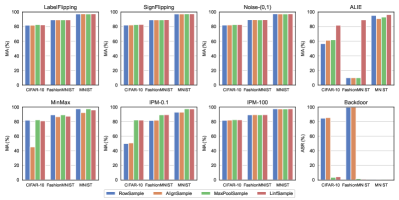
Figure 5: The MA and ASR (%) of the three baselines and $\mathsf{LinfSample}$ across three datasets.

To demonstrate the superior resistance of $\mathsf{LinfSample}$ against Byzantine attacks and its capability to reduce the SMPC overhead of computing shared SED matrix, we compared it with three other sampling methods, ensuring that the subsequent voting process is consistent with FLUD. The specific configurations for the four methods are as follows:

(i) $\mathsf{RowSample}$: No sampling is performed. Servers compute the shared SED matrix on updates. (ii) $\mathsf{AlignSample}$ [35]: For each layer of the update, the maximum absolute value is determined first, and all entries are aligned with this value while retaining their original signs. The output of this process serves as the update digest. (iii) $\mathsf{MaxPoolSample}$ [42]: The update is reshaped into a matrix and subjected to 2D max-pooling with a kernel size of $5\times 5$ to compute the update digest. (iv) $\mathsf{LinfSample}$: The update is computed as described in Sec. IV-B1, with the window size set to $4096$. In (ii), (iii) and (iv), servers compute the shared SED matrix on digests.

VI-B1 Byzantine resilience

Our results in Fig. 5 indicate that in the presence of straightforward attacks such as LabelFlipping, SignFlipping, Noise-(0,1), and IPM-100, all four sampling methods are capable of effectively identifying poisoned updates.

When training on the MNIST, the structure of the global model is the simplest, and all methods are capable of withstanding the four other types of attacks. However, when the global model becomes more complex, all methods show a slight decline in their defensive capabilities against Backdoor. Concurrently, the ALIE can easily compromise the global models using ResNet10 and FashionCNN across three baselines. Both $\mathsf{RowSample}$ and $\mathsf{AlignSample}$ also fail under the IPM-0.1 and Backdoor when the global model employs ResNet10 or FashionCNN. These observations underscore that despite the escalating complexity of both the global models and the attacks, the updates maintain variability in their segmented $l_{\infty}$. Consequently, $\mathsf{LinfSample}$ demonstrates a more robust capability to resist interference from fine-tuning updates compared to other sampling methods.

VI-B2 Communication of client uploads for Sharing

The $\mathsf{RowSample}$ method requires only the splitting of updates, resulting in the lowest overhead for client-side sharing. In contrast, $\mathsf{LinfSample}$, $\mathsf{AlignSample}$, and $\mathsf{MaxPoolSample}$ additionally necessitate the splitting of digests. Consequently, the size of these digests determines the additional overhead that clients must bear. According to Tab. II, the digests produced by $\mathsf{LinfSample}$ are the shortest among the three methods, thus rendering the extra overhead imposed on clients by $\mathsf{LinfSample}$ negligible.

VI-B3 Overhead of computing SED matrix

TABLE II: Comparison of the overhead imposed on clients and servers by $\mathsf{LinfSample}$ and three other sampling methods.

Dataset $\mathsf{RowSample}$ $\mathsf{AlignSample}$ $\mathsf{MaxPoolSample}$ $\mathsf{LinfSample}$ Communication of sharing for each client (MB) CIFAR-10 374.1 748.2 389.1 374.2 FashionMNIST 112.5 225.1 117.1 112.6 MNIST 10.4 20.8 10.8 10.4 Communication of computing shared SED matrix for servers (MB) CIFAR-10 14215.3 14215.3 568.6 3.5 FashionMNIST 4276.7 4276.7 171.1 1.1 MNIST 394.5 394.5 15.8 0.1 Runtime of computing shared SED matrix for servers (s) CIFAR-10 5757.2 5757.2 217.5 3.2 FashionMNIST 1752.0 1752.0 74.3 1.8 MNIST 154.7 154.7 11.7 1.0

We further test the communication and time overhead of computing the SED matrix for the four sampling methods, which are depicted in Tab. II. The ppBRARs employing these four methods compute the same number of SEDs. The overhead is primarily dependent on the length of the input shared vectors. The length of $\langle\boldsymbol{g}_{i}\rangle$ is identical to that of $\langle\boldsymbol{d}_{i}\rangle$ in $\mathsf{AlignSample}$, $25$ times that of $\langle\boldsymbol{d}_{i}\rangle$ in $\mathsf{MaxPoolSample}$, and $4096$ times that of $\langle\boldsymbol{d}_{i}\rangle$ in $\mathsf{LinfSample}$. Observations in Tab. II indicate that FLUD reduces communication and runtime by three orders of magnitude compared to $\mathsf{RowSample}$ and $\mathsf{AlignSample}$. Simultaneously, compared to $\mathsf{MaxPoolSample}$, $\mathsf{RowSample}$ also demonstrates a significant overhead advantage.

VI-C Byzantine Robustness of FLUD

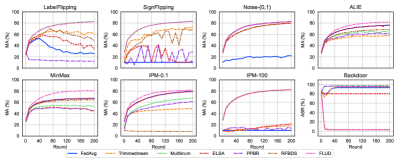
(a) The dataset is CIFAR-10, the global model is ResNet10.

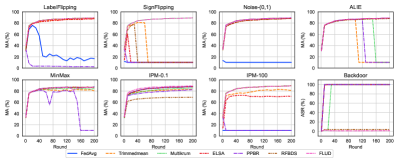
(b) The dataset is FashionMNIST, the global model is FashionCNN.

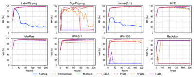
(c) The dataset is MNIST, the global model is MNIST-MLP.

Figure 6: Under the scenario with a 40% malicious client ratio, MA and ASR (%) of FLUD and the other six comparative schemes against Byzantine attacks across three datasets.

We evaluate the Byzantine resilience of six baselines and FLUD:

• FedAvg [1]: Aggregates updates by taking the weighted average.

• Trimmedmean [12]: Removes the highest and lowest 40% of values in each dimension and takes the average of the remaining values.

• Multikrum [10]: The server calculates the sum of Euclidean distances to the 10 nearest neighbors of $\boldsymbol{g}_{i}$, using this sum as a score. The smaller the score, the higher the credibility, and the server aggregates the updates of the 10 smallest scores.

• ELSA [28]: Assumes that the server knows an ideal norm, which is the average of the norms of model updates from all benign clients. Any update larger than the ideal norm is clipped to the ideal norm.

• PPBR [25]: Calculates the sum of cosine similarities to the $10$ nearest neighbors of $\boldsymbol{g}_{i}$ as a credibility score, and finally aggregates the $10$ updates with the highest credibility scores.

• RFBDS[35]: Compresses updates using $\mathsf{AlignSample}$, clusters them with OPTICS, and clips the updates using $l_{2}$ norm.

We plot the Byzantine resilience of the baselines and FLUD under three datasets in Fig. 6, where all datasets are IID. We find that as the model becomes more complex, some aggregation schemes, when faced with ALIE, MinMax, and IPM-0.1 attacks, converge to lower accuracy or even fail. Only FLUD consistently maintains the highest accuracy, indicating that $\mathsf{LinfSample}$ can capture the differences in poisoned updates under such attacks by sampling on $l_{\infty}$. Additionally, adversaries implementing Noise attacks are easily defended by aggregation methods other than FedAvg. We found that only RFBDS and FLUD can effectively resist Backdoor attacks. Multikrum and FLUD can effectively resist LabelFlipping, SignFlipping, and IPM-100 attacks. Overall, FLUD has surprisingly robust Byzantine resilience.

VI-D Influence of Window Size

TABLE III: The MA and ASR (%) of $\mathsf{LinfSample}$ against Byzantine attacks with different sizes of sampling windows.

Dataset (No. of Model Parameters) Attack The size of the sampling window.($2^{X}$) 4 5 6 7 8 9 10 11 12 13 14 15 16 17 18 19 20 21 22 23 CIFAR-10 ($4,903,242$) ALIE $81.5$ $81.7$ $81.5$ $81.8$ $81.9$ $82.0$ $82.0$ $82.1$ $81.9$ $82.0$ $81.8$ $82.1$ $82.2$ $82.0$ $82.2$ $82.1$ $82.0$ $81.3$ $81.2$ $80.9$ LabelFlipping $82.8$ $82.4$ $82.2$ $82.3$ $82.4$ $82.5$ $82.8$ $82.7$ $82.3$ $82.7$ $82.7$ $82.7$ $82.4$ $82.4$ $82.8$ $82.3$ $82.4$ $82.7$ $82.5$ $72.6$ Noise-(0,1) $82.3$ $82.5$ $82.3$ $82.5$ $82.7$ $82.8$ $82.3$ $82.7$ $82.8$ $82.7$ $82.1$ $83.0$ $82.9$ $82.5$ $82.6$ $82.7$ $82.9$ $82.6$ $82.8$ $82.9$ SignFlipping $82.5$ $82.6$ $82.6$ $82.7$ $82.6$ $82.6$ $82.5$ $82.9$ $82.9$ $82.6$ $82.7$ $82.5$ $82.7$ $82.8$ $82.4$ $82.8$ $82.7$ $82.6$ $82.7$ $83.2$ MinMax $61.6$ $60.7$ $61.4$ $57.4$ $73.4$ $80.4$ $80.6$ $81.0$ $81.1$ $81.4$ $81.7$ $81.3$ $81.5$ $81.0$ $73.9$ $72.4$ $70.9$ $69.2$ $71.5$ $68.1$ IPM-0.1 $81.8$ $82.0$ $81.5$ $81.7$ $81.9$ $82.0$ $81.8$ $82.0$ $82.0$ $81.8$ $81.6$ $82.0$ $81.8$ $82.3$ $82.4$ $82.2$ $82.3$ $82.4$ $82.0$ $82.4$ IPM-100 $82.4$ $82.3$ $82.3$ $82.3$ $82.5$ $82.4$ $82.4$ $82.3$ $82.4$ $82.5$ $82.3$ $82.4$ $82.2$ $82.6$ $82.7$ $82.4$ $82.3$ $82.5$ $82.6$ $82.7$ Backdoor(ASR) 25.21 14.2 3.6 8.57 3.74 3.74 3.34 3.78 4.15 3.52 3.45 3.97 3.6 4.0 4.38 3.82 5.12 3.86 7.04 48.09 FashionMNIST ($1,475,146$) ALIE $88.9$ $88.9$ $89.2$ $89.2$ $89.2$ $89.3$ $89.3$ $89.3$ $89.3$ $89.3$ $89.3$ $89.3$ $89.2$ $89.2$ $89.1$ $89.1$ $89.1$ $89.2$ - - LabelFlipping $89.3$ $89.3$ $89.3$ $89.3$ $89.4$ $89.3$ $89.4$ $89.5$ $89.3$ $89.5$ $89.4$ $89.4$ $89.4$ $89.4$ $89.2$ $89.3$ $89.3$ $89.4$ - - Noise-(0,1) $89.4$ $89.4$ $89.2$ $89.4$ $89.3$ $89.4$ $89.4$ $89.4$ $89.4$ $89.4$ $89.4$ $89.4$ $89.3$ $89.2$ $89.3$ $89.3$ $89.2$ $89.4$ - - SignFlipping $89.3$ $89.3$ $89.3$ $89.3$ $89.2$ $89.3$ $89.3$ $89.4$ $89.4$ $89.4$ $89.3$ $89.3$ $89.3$ $89.3$ $89.3$ $89.4$ $89.3$ $89.3$ - - MinMax $83.8$ $85.8$ $83.8$ $84.9$ $86.0$ $86.4$ $85.9$ $86.5$ $87.4$ $86.4$ $84.7$ $85.3$ $87.7$ $87.1$ $86.4$ $84.9$ $84.7$ $85.1$ - - IPM-0.1 $89.3$ $89.3$ $89.3$ $89.3$ $89.3$ $89.4$ $89.4$ $89.4$ $89.4$ $89.4$ $89.5$ $89.4$ $89.4$ $89.4$ $89.4$ $89.3$ $89.4$ $89.3$ - - IPM-100 $89.3$ $89.3$ $89.4$ $89.4$ $89.3$ $89.4$ $89.4$ $89.4$ $89.4$ $89.4$ $89.4$ $89.4$ $89.3$ $89.3$ $89.3$ $89.5$ $89.3$ $89.4$ - - Backdoor(ASR) $1.0$ $1.2$ $1.1$ $1.2$ $1.2$ $1.3$ $1.4$ $1.2$ $1.4$ $1.6$ $1.3$ $1.0$ $1.3$ $1.4$ $1.2$ $1.1$ $8.2$ $100.0$ - - MNIST ($136,074$) ALIE $93.6$ $94.1$ $94.8$ $95.0$ $95.4$ $96.0$ $96.3$ $96.5$ $96.4$ $96.7$ $96.0$ $95.7$ $96.0$ $95.1$ $91.2$ - - - - - LabelFlipping $97.5$ $97.4$ $97.4$ $97.5$ $97.4$ $97.4$ $97.5$ $97.4$ $97.5$ $97.4$ $97.5$ $97.4$ $97.4$ $97.5$ $97.5$ - - - - - Noise-(0,1) $97.4$ $97.5$ $97.5$ $97.4$ $97.4$ $97.5$ $97.4$ $97.4$ $97.4$ $97.5$ $97.5$ $97.5$ $97.5$ $97.5$ $97.5$ - - - - - SignFlipping $97.4$ $97.4$ $97.4$ $97.5$ $97.5$ $97.4$ $97.5$ $97.4$ $97.5$ $97.4$ $97.5$ $97.6$ $97.5$ $97.5$ $97.5$ - - - - - MinMax $93.6$ $94.3$ $94.5$ $94.6$ $94.9$ $95.3$ $95.5$ $95.8$ $95.9$ $96.1$ $96.4$ $96.4$ $96.4$ $96.2$ $96.0$ - - - - - IPM-0.1 $97.4$ $97.4$ $97.4$ $97.3$ $97.3$ $97.4$ $97.3$ $97.4$ $97.3$ $97.4$ $97.3$ $97.4$ $97.4$ $97.4$ $97.4$ - - - - - IPM-100 $97.4$ $97.5$ $97.5$ $97.4$ $97.4$ $97.4$ $97.4$ $97.4$ $97.5$ $97.4$ $97.5$ $97.5$ $97.5$ $97.6$ $97.5$ - - - - - Backdoor(ASR) $0.2$ $0.1$ $0.2$ $0.2$ $0.2$ $0.2$ $0.2$ $0.2$ $0.1$ $0.2$ $0.3$ $0.2$ $0.2$ $0.2$ $0.2$ - - - - -

Intuitively, when the size of the sampling window, $2^{X}$, in $\mathsf{LinfSample}$ is too small, detecting changes in the signs of poisoned model updates may be challenging. Conversely, when $2^{X}$ is excessively large, it may result in significant information loss. The test results are presented in Tab. III. We observed that the attacks most sensitive to the size of $2^{X}$ are LabelFlipping, ALIE, MinMax, and Backdoor attacks. This observation is consistent with our discussion in Sec. IV-A. To ensure that FLUD can effectively filter Mix-scaled Updates when training global models with varying architectures, selecting an appropriate size for the sampling window is crucial. Based on an empirical analysis of the experimental results, setting the window size to $2^{11}$, $2^{12}$, $2^{13}$, or $2^{14}$ is reasonable. The updates generated by the other four simpler attacks fall into either Up-scaled Updates or Down-scaled Updates categories; therefore, FLUD’s resilience against these attacks is not sensitive to the size of the sampling window in $\mathsf{LinfSample}$.

VI-E Impact of Client Data Distribution

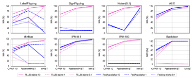
Figure 7: The MA and ASR (%) of the FedAvg and FLUD across three different data distributions.

Furthermore, we utilize the same Dirichlet distribution as in [43] to partition the training set. A smaller value of $\alpha$ indicates a greater degree of non-IIDness, leading clients to likely possess samples predominantly from a single category. Conversely, a larger $\alpha$ results in more similar data distributions across clients. We test three different settings of $\alpha$: 10, 1, and 0.1 and the experimental results are presented in Fig. 7.

It is evident that at $\alpha=10$, FLUD is the most robust under all attack scenarios. At $\alpha=1$, FLUD still maintains higher robustness in most scenarios compared to FedAvg. However, in CIFAR-10, under LabelFlipping, ALIE, and MinMax attacks, FLUD shows some instability as it slightly underperforms compared to FedAvg. When $\alpha$ is reduced to 0.1, due to increased distances between model updates of benign clients, FLUD exhibits more instability, leading to its underperformance in ALIE, MinMax, and IPM-0.1 attacks compared to FedAvg.

Therefore, FLUD demonstrates sufficient robustness when $\alpha$ is high. However, as $\alpha$ decreases, its ability to filter out malicious clients in attacks such as LabelFlipping, ALIE, MinMax, and Backdoor gradually declines.

VI-F Efficiency of Computing Medians

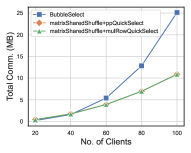
(a) Communication

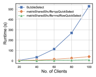
(b) Runtime

Figure 8: Overheads of computing medians for servers.

To further compute the medians of all rows in SED matrix, we compare $\mathsf{matrixSharedShuffle+mulRowQuickSelect}$ with two other baselines. The $\mathsf{BubbleSelect}$ protocol employs privacy-preserving maxpooling from [20] and utilizes bubble sort to find the $m/2$ largest shared value row-by-row. The $\mathsf{matrixSharedShuffle+ppQuickSelect}$ protocol employs the same shuffle algorithm as FLUD and utilizes the select method from [4] to compute the shared median row-by-row. The overhead of these three protocols is solely dependent on the number of clients, i.e., the size of the distance matrix. Therefore, we test the communication and runtime of the three protocols with 20, $40$, $60$, $80$, and $100$ clients.

To find the median of a row, the comparison complexity of $\mathsf{BubbleSelect}$ is $O(m^{3})$, while the comparison complexity of the other two protocols is $O(m)$. Furthermore, when the goal is to find the medians of multiple rows, $\mathsf{mulRowQuickSelect}$ packs and compares the shares in multiple rows each time until it finds the medians of all rows. As such, when calculating the medians of multiple sequences, its worst-case comparison complexity is $O(m^{2})$, and the average comparison complexity is $O(m)$. In contrast, the average comparison complexity of $\mathsf{ppQuickSelect}$ is $O(m^{2})$.

From Fig. 8a, it can be observed that the communication overhead of the three protocols is nearly identical when the number of clients is $20$ and $40$. As the number of clients increases, although $\mathsf{BubbleSelect}$ does not require row shuffling, its overhead grows the fastest. In contrast, the communication costs of the other two protocols increase more gradually. When the client count reaches 100, the communication overhead of $\mathsf{BubbleSelect}$ becomes twice that of the other two protocols. From Fig. 8b, it is evident that when the number of clients is $20$, the runtime of the three protocols is essentially the same. Moreover, as the number of clients increases, the runtime overhead of using $\mathsf{mulRowQuickSelect}$ consistently remains the lowest and increases most slowly.

VII Conclusion

This study introduces FLUD framework, enhancing data security, privacy, and access control in distributed environments. FLUD employs update digests and a novel, privacy-preserving, voting-based defense to mitigate risks posed by Byzantine adversaries, significantly reducing the computational and communication overhead associated with SMPC. Since we assume a relatively weak adversary who does not forge update digests, FLUD does not incorporate steps for verifying update digests. Future work will focus on developing methods to verify update digests efficiently, even in the presence of stronger adversaries, thus broadening FLUD’s applicability and robustness against more sophisticated threats. Overall, this framework contributes to improving the robustness of FL systems against security threats, ensuring safer data management practices in AI applications.

Wenjie Li received his M.S. degree from the School of Cyber Security and Computer, Hebei University of China in 2021. Currently, he is a Ph.D. student at the School of Cyber Engineering, Xidian University, China, and also a visiting student at the College of Computing and Data Science (CCDS) at Nanyang Technological University (NTU). He is working on cryptography, secure aggregation in federated learning and privacy-preserving machine learning.

Kai Fan received his B.S., M.S. and Ph.D. degrees from Xidian University, P.R.China, in 2002, 2005 and 2007, respectively, in Telecommunication Engineering, Cryptography and Telecommunication and Information System. He is working as a professor in State Key Laboratory of Integrated Service Networks at Xidian University. He published over 70 papers in journals and conferences. He received 9 Chinese patents. He has managed 5 national research projects. His research interests include IoT security and information security.

Jingyuan Zhang received the B.Eng. degree in cyber space security from the School of Cyber Science and Engineering, Wuhan University. He is currently pursuing a Master of Science in Artificial Intelligence at the College of Computing and Data Science (CCDS) at Nanyang Technological University (NTU). His research interests include federated learning and federated transfer learning.

Hui Li was born in 1968 in Shaanxi Province of China. In 1990, he received his B. S. degree in radio electronics from Fudan University. In 1993, and 1998, he received his M.S. degree and Ph.D. degree in telecommunications and information system from Xidian University respectively. He is now a professor of Xidian University. His research interests include network and information security.

Wei Yang Bryan Lim is currently an Assistant Professor at the College of Computing and Data Science (CCDS), Nanyang Technological University (NTU), Singapore. Previously, he was Wallenberg-NTU Presidential Postdoctoral Fellow. In 2022, he earned his PhD from NTU under the Alibaba PhD Talent Programme and was affiliated with the CityBrain team of DAMO academy. His doctoral efforts earned him accolades such as the “Most Promising Industrial Postgraduate Programme Student” award and the IEEE Technical Community on Scalable Computing (TCSC) Outstanding PhD Dissertation Award. He has also won the best paper awards, notably from the IEEE Wireless Communications and Networking Conference (WCNC) and the IEEE Asia Pacific Board. He serves on the Technical Programme Committee for FL workshops at flagship conferences (AAAI-FL, IJCAI-FL) and is a review board member for reputable journals like the IEEE Transactions on Parallel and Distributed Systems. In 2023, he co-edited a submission on “Requirements and Design Criteria for Sustainable Metaverse Systems” for the International Telecommunication Union (ITU). He has also been a visiting scholar at various institutions such as the University of Tokyo, KTH Royal Institute of Technology, and the University of Sydney.

Qiang Yang is a Fellow of Canadian Academy of Engineering (CAE) and Royal Society of Canada (RSC), Chief Artificial Intelligence Officer of WeBank, a Chair Professor of Computer Science and Engineering Department at Hong Kong University of Science and Technology (HKUST). He is theConference Chair of AAAI-21, the Honorary Vice President of Chinese Association for Artificial Intelligence(CAAI) , the President of Hong Kong Society of Artificial Intelligence and Robotics (HKSAIR)and the President of Investment Technology League (ITL). He is a fellow of AAAI, ACM, CAAI, IEEE, IAPR, AAAS. He was the Founding Editor in Chief of the ACM Transactions on Intelligent Systems and Technology (ACM TIST) and the Founding Editor in Chief of IEEE Transactions on Big Data (IEEE TBD). He received the ACM SIGKDD Distinguished Service Award in 2017. He had been the Founding Director of the Huawei’s Noah’s Ark Research Lab between 2012 and 2015, the Founding Director of HKUST’s Big Data Institute, the Founder of 4Paradigm and the President of IJCAI (2017-2019). His research interests are artificial intelligence, machine learning, data mining and planning.

References

- [1] Brendan McMahan, Eider Moore, Daniel Ramage, Seth Hampson, and Blaise Aguera y Arcas. Communication-Efficient Learning of Deep Networks from Decentralized Data. In Aarti Singh and Jerry Zhu, editors, Proceedings of the 20th International Conference on Artificial Intelligence and Statistics, volume 54 of Proceedings of Machine Learning Research, pages 1273–1282. PMLR, 20–22 Apr 2017.
- [2] Jiannan Cai, Zhidong Gao, Yuanxiong Guo, Bastian Wibranek, and Shuai Li. Fedhip: Federated learning for privacy-preserving human intention prediction in human-robot collaborative assembly tasks. Advanced Engineering Informatics, 60:102411, 2024.
- [3] Zhuoran Ma, Jianfeng Ma, Yinbin Miao, Yingjiu Li, and Robert H Deng. Shieldfl: Mitigating model poisoning attacks in privacy-preserving federated learning. IEEE Transactions on Information Forensics and Security, 17:1639–1654, 2022.
- [4] Wenjie Li, Kai Fan, Kan Yang, Yintang Yang, and Hui Li. Pbfl: Privacy-preserving and byzantine-robust federated learning empowered industry 4.0. IEEE Internet of Things Journal, 2023.
- [5] Xiaoyu Cao, Minghong Fang, Jia Liu, and Neil Zhenqiang Gong. Fltrust: Byzantine-robust federated learning via trust bootstrapping. In 28th Annual Network and Distributed System Security Symposium, NDSS 2021, virtually, February 21-25, 2021. The Internet Society, 2021.
- [6] Ye Dong, Xiaojun Chen, Kaiyun Li, Dakui Wang, and Shuai Zeng. FLOD: oblivious defender for private byzantine-robust federated learning with dishonest-majority. In Elisa Bertino, Haya Schulmann, and Michael Waidner, editors, Computer Security - ESORICS 2021 - 26th European Symposium on Research in Computer Security, Darmstadt, Germany, October 4-8, 2021, Proceedings, Part I, volume 12972 of Lecture Notes in Computer Science, pages 497–518. Springer, 2021.
- [7] Virat Shejwalkar and Amir Houmansadr. Manipulating the byzantine: Optimizing model poisoning attacks and defenses for federated learning. In NDSS, 2021.
- [8] Ziteng Sun, Peter Kairouz, Ananda Theertha Suresh, and H. Brendan McMahan. Can you really backdoor federated learning? CoRR, abs/1911.07963, 2019.
- [9] Eugene Bagdasaryan, Andreas Veit, Yiqing Hua, Deborah Estrin, and Vitaly Shmatikov. How to backdoor federated learning. In Silvia Chiappa and Roberto Calandra, editors, Proceedings of the Twenty Third International Conference on Artificial Intelligence and Statistics, volume 108 of Proceedings of Machine Learning Research, pages 2938–2948. PMLR, 26–28 Aug 2020.
- [10] Peva Blanchard, El Mahdi El Mhamdi, Rachid Guerraoui, and Julien Stainer. Machine learning with adversaries: Byzantine tolerant gradient descent. In I. Guyon, U. Von Luxburg, S. Bengio, H. Wallach, R. Fergus, S. Vishwanathan, and R. Garnett, editors, Advances in Neural Information Processing Systems, volume 30. Curran Associates, Inc., 2017.
- [11] Malhar S Jere, Tyler Farnan, and Farinaz Koushanfar. A taxonomy of attacks on federated learning. IEEE Security & Privacy, 19(2):20–28, 2020.
- [12] Dong Yin, Yudong Chen, Ramchandran Kannan, and Peter Bartlett. Byzantine-robust distributed learning: Towards optimal statistical rates. In Jennifer Dy and Andreas Krause, editors, Proceedings of the 35th International Conference on Machine Learning, volume 80 of Proceedings of Machine Learning Research, pages 5650–5659. PMLR, 10–15 Jul 2018.
- [13] Xinyu Zhang, Qingyu Liu, Zhongjie Ba, Yuan Hong, Tianhang Zheng, Feng Lin, Li Lu, and Kui Ren. Fltracer: Accurate poisoning attack provenance in federated learning, 2023.
- [14] Ligeng Zhu, Zhijian Liu, and Song Han. Deep leakage from gradients. In H. Wallach, H. Larochelle, A. Beygelzimer, F. d'Alché-Buc, E. Fox, and R. Garnett, editors, Advances in Neural Information Processing Systems, volume 32. Curran Associates, Inc., 2019.
- [15] Bo Zhao, Konda Reddy Mopuri, and Hakan Bilen. idlg: Improved deep leakage from gradients. CoRR, abs/2001.02610, 2020.
- [16] Jonas Geiping, Hartmut Bauermeister, Hannah Dröge, and Michael Moeller. Inverting gradients - how easy is it to break privacy in federated learning? In H. Larochelle, M. Ranzato, R. Hadsell, M.F. Balcan, and H. Lin, editors, Advances in Neural Information Processing Systems, volume 33, pages 16937–16947. Curran Associates, Inc., 2020.
- [17] Hongsheng Hu, Zoran Salcic, Lichao Sun, Gillian Dobbie, and Xuyun Zhang. Source inference attacks in federated learning. In 2021 IEEE International Conference on Data Mining (ICDM), pages 1102–1107. IEEE, 2021.
- [18] Kai Yue, Richeng Jin, Chau-Wai Wong, Dror Baron, and Huaiyu Dai. Gradient obfuscation gives a false sense of security in federated learning. In Joseph A. Calandrino and Carmela Troncoso, editors, 32nd USENIX Security Symposium, USENIX Security 2023, Anaheim, CA, USA, August 9-11, 2023, pages 6381–6398. USENIX Association, 2023.
- [19] Daniel Demmler, Thomas Schneider, and Michael Zohner. Aby-a framework for efficient mixed-protocol secure two-party computation. In NDSS, 2015.
- [20] Deevashwer Rathee, Mayank Rathee, Nishant Kumar, Nishanth Chandran, Divya Gupta, Aseem Rastogi, and Rahul Sharma. Cryptflow2: Practical 2-party secure inference. In Proceedings of the 2020 ACM SIGSAC Conference on Computer and Communications Security, pages 325–342, 2020.
- [21] Shenghui Li, Edith Ngai, Fanghua Ye, Li Ju, Tianru Zhang, and Thiemo Voigt. Blades: A unified benchmark suite for byzantine attacks and defenses in federated learning. In 2024 IEEE/ACM Ninth International Conference on Internet-of-Things Design and Implementation (IoTDI), 2024.
- [22] Shenghui Li, Edith C.-H. Ngai, and Thiemo Voigt. An experimental study of byzantine-robust aggregation schemes in federated learning. IEEE Transactions on Big Data, pages 1–13, 2023.
- [23] Torsten Krauß and Alexandra Dmitrienko. Mesas: Poisoning defense for federated learning resilient against adaptive attackers. In Proceedings of the 2023 ACM SIGSAC Conference on Computer and Communications Security, CCS ’23, page 1526–1540, New York, NY, USA, 2023. Association for Computing Machinery.
- [24] Ning Wang, Yang Xiao, Yimin Chen, Yang Hu, Wenjing Lou, and Y Thomas Hou. Flare: defending federated learning against model poisoning attacks via latent space representations. In Proceedings of the 2022 ACM on Asia Conference on Computer and Communications Security, pages 946–958, 2022.
- [25] Caiqin Dong, Jian Weng, Ming Li, Jia-Nan Liu, Zhiquan Liu, Yudan Cheng, and Shui Yu. Privacy-preserving and byzantine-robust federated learning. IEEE Transactions on Dependable and Secure Computing, 2023.
- [26] Xicong Shen, Ying Liu, Fu Li, and Chunguang Li. Privacy-preserving federated learning against label-flipping attacks on non-iid data. IEEE Internet of Things Journal, 2023.
- [27] Hidde Lycklama, Lukas Burkhalter, Alexander Viand, Nicolas Küchler, and Anwar Hithnawi. Rofl: Robustness of secure federated learning. In 44th IEEE Symposium on Security and Privacy, SP 2023, San Francisco, CA, USA, May 21-25, 2023, pages 453–476. IEEE, 2023.
- [28] Mayank Rathee, Conghao Shen, Sameer Wagh, and Raluca Ada Popa. ELSA: secure aggregation for federated learning with malicious actors. In 44th IEEE Symposium on Security and Privacy, SP 2023, San Francisco, CA, USA, May 21-25, 2023, pages 1961–1979. IEEE, 2023.
- [29] Jian Xu, Shao-Lun Huang, Linqi Song, and Tian Lan. Byzantine-robust federated learning through collaborative malicious gradient filtering. In 2022 IEEE 42nd International Conference on Distributed Computing Systems (ICDCS), pages 1223–1235. IEEE, 2022.
- [30] Liping Li, Wei Xu, Tianyi Chen, Georgios B Giannakis, and Qing Ling. Rsa: Byzantine-robust stochastic aggregation methods for distributed learning from heterogeneous datasets. In Proceedings of the AAAI conference on artificial intelligence, volume 33, pages 1544–1551, 2019.
- [31] Gilad Baruch, Moran Baruch, and Yoav Goldberg. A little is enough: Circumventing defenses for distributed learning. Advances in Neural Information Processing Systems, 32, 2019.
- [32] Virat Shejwalkar and Amir Houmansadr. Manipulating the byzantine: Optimizing model poisoning attacks and defenses for federated learning. In NDSS, 2021.
- [33] Cong Xie, Oluwasanmi Koyejo, and Indranil Gupta. Fall of empires: Breaking byzantine-tolerant sgd by inner product manipulation. In Ryan P. Adams and Vibhav Gogate, editors, Proceedings of The 35th Uncertainty in Artificial Intelligence Conference, volume 115 of Proceedings of Machine Learning Research, pages 261–270. PMLR, 22–25 Jul 2020.
- [34] Pascal Paillier. Public-key cryptosystems based on composite degree residuosity classes. In International conference on the theory and applications of cryptographic techniques, pages 223–238. Springer, 1999.
- [35] Zekai Chen, Shengxing Yu, Mingyuan Fan, Ximeng Liu, and Robert H Deng. Privacy-enhancing and robust backdoor defense for federated learning on heterogeneous data. IEEE Transactions on Information Forensics and Security, 2023.
- [36] Yehuda Lindell. How to simulate it–a tutorial on the simulation proof technique. Tutorials on the Foundations of Cryptography: Dedicated to Oded Goldreich, pages 277–346, 2017.
- [37] Koki Hamada, Ryo Kikuchi, Dai Ikarashi, Koji Chida, and Katsumi Takahashi. Practically efficient multi-party sorting protocols from comparison sort algorithms. In Information Security and Cryptology–ICISC 2012: 15th International Conference, Seoul, Korea, November 28-30, 2012, Revised Selected Papers 15, pages 202–216. Springer, 2013.
- [38] Jinguo Li, Yan Yan, Kai Zhang, Chunlin Li, and Peichun Yuan. Fpcnn: A fast privacy-preserving outsourced convolutional neural network with low-bandwidth. Knowledge-Based Systems, 283:111181, 2024.
- [39] Alex Krizhevsky, Vinod Nair, and Geoffrey Hinton. Cifar-10 (canadian institute for advanced research).
- [40] Han Xiao, Kashif Rasul, and Roland Vollgraf. Fashion-mnist: a novel image dataset for benchmarking machine learning algorithms. arXiv preprint arXiv:1708.07747, 2017.
- [41] Yann LeCun, Léon Bottou, Yoshua Bengio, and Patrick Haffner. Gradient-based learning applied to document recognition. Proceedings of the IEEE, 86(11):2278–2324, 1998.
- [42] Zirui Gong, Liyue Shen, Yanjun Zhang, Leo Yu Zhang, Jingwei Wang, Guangdong Bai, and Yong Xiang. Agramplifier: Defending federated learning against poisoning attacks through local update amplification. IEEE Transactions on Information Forensics and Security, 19:1241–1250, 2023.
- [43] Tao Lin, Lingjing Kong, Sebastian U Stich, and Martin Jaggi. Ensemble distillation for robust model fusion in federated learning. Advances in Neural Information Processing Systems, 33:2351–2363, 2020.