Federated Q-Learning with Reference-Advantage Decomposition: Almost Optimal Regret and Logarithmic Communication Cost

Abstract

In this paper, we consider model-free federated reinforcement learning for tabular episodic Markov decision processes. Under the coordination of a central server, multiple agents collaboratively explore the environment and learn an optimal policy without sharing their raw data. Despite recent advances in federated Q-learning algorithms achieving near-linear regret speedup with low communication cost, existing algorithms only attain suboptimal regrets compared to the information bound. We propose a novel model-free federated Q-learning algorithm, termed FedQ-Advantage. Our algorithm leverages reference-advantage decomposition for variance reduction and operates under two distinct mechanisms: synchronization between the agents and the server, and policy update, both triggered by events. We prove that our algorithm not only requires a lower logarithmic communication cost but also achieves an almost optimal regret, reaching the information bound up to a logarithmic factor and near-linear regret speedup compared to its single-agent counterpart when the time horizon is sufficiently large.

1 Introduction

Federated reinforcement learning (FRL) is a distributed learning framework that combines the principles of reinforcement learning (RL) [1] and federated learning (FL) [2]. Focusing on sequential decision-making, FRL aims to learn an optimal policy through parallel explorations by multiple agents under the coordination of a central server. Often modeled as a Markov decision process (MDP), multiple agents independently interact with an initially unknown environment and collaboratively train their decision-making models with limited information exchange between the agents. This approach accelerates the learning process with low communication costs. Some model-based algorithms (e.g., [3]) and policy-based algorithms (e.g., [4]) have shown speedup with respect to the number of agents in terms of learning regret or convergence rate. Recent progress has been made in FRL algorithms based on model-free value-based approaches, which directly learn the value functions and the optimal policy without estimating the underlying model (e.g., [5]). However, most existing model-free federated algorithms do not actively update the exploration policies for local agents and fail to provide low regret. A comprehensive literature review is provided in Appendix A.

1.1 Federated Q-learning: prior works and limitations

In this paper, we focus on model-free FRL based on the classic Q-learning algorithm [6], tailored for episodic tabular MDPs with inhomogeneous transition kernels. Specifically, we assume the presence of a central server and $M$ local agents in the system. Each agent interacts independently with an episodic MDP consisting of $S$ states, $A$ actions, and $H$ steps per episode.

Let $T$ denote the number of steps for each agent. Under the single-agent setting of the episodic MDP, [7] and [8] established a lower bound for the expected total regret of $\Omega(\sqrt{H^{2}SAT})$. An algorithm is considered almost optimal when it achieves a regret upper bound of $\tilde{O}(\sqrt{H^{2}SAT})$ for large values of $T$. Multiple model-based algorithms (e.g., [9]) have been shown to be almost optimal. Research on provably efficient model-free algorithms began with [8] and was further advanced by [10, 11, 12]. Specifically, [11, 12] proposed almost optimal algorithms that utilized reference-advantage decomposition for variance reduction.

For the federated setting, the information bound naturally translates to $\Omega(\sqrt{H^{2}SAMT})$, allowing us to define almost optimal federated algorithms similarly. However, the literature on federated model-free algorithms is quite limited. [10] and [11] proposed concurrent algorithms where multiple agents generate episodes simultaneously and share their original data with the central server. These designs achieved low policy-switching costs but incurred a high communication cost of $O(MT)$ due to full dataset sharing. [13] proposed federated algorithms with near-linear regret speedup compared to [8] and [10] and logarithmic communication cost, but they only achieved a suboptimal regret upper bound of $\tilde{O}(\sqrt{MH^{3}SAT})$. This raises the following question:

Is it possible to design an almost optimal federated model-free RL algorithm that enjoys a logarithmic communication cost?

1.2 Summary of our contributions

We give an affirmative answer to this question by proposing the algorithm FedQ-Advantage and summarize our main contributions below.

• Algorithmic design. In FedQ-Advantage, the server coordinates the agents by actively updating their exploration policies, while the agents execute these policies, collect trajectories, and periodically share local aggregations with the server to form global updates and refine the exploration policy. The algorithm features the following elements in its design:

  (1) Upper confidence bounds (UCB) and reference-advantage decomposition. In addition to using UCB adopted by existing algorithms to promote exploration, we decompose the state value function into a reference value function and an advantage function for variance reduction when updating the $Q$-function, similar to [11] and [12]. Both functions are updated periodically in the federated algorithm. This decomposition is key to achieving almost optimal regret.

  (2) Separate mechanisms for event-triggered synchronization and policy switching. To reduce communication cost, we use separate mechanisms for event-triggered policy switching and synchronization, which occur only when certain conditions are met. This partitions the learning process into rounds that are further grouped into stages. Synchronization occurs at the end of each round while policy switching and updates of estimated $Q$-functions only occur at the end of a stage. This approach differs from the federated algorithms in [13], which used the same mechanism for triggering policy switching and synchronization. When updating the estimated $Q$-functions for a given state-action-step tuple, we assign equal weights to all new visits to the tuple within the current stage. Consequently, local agents only need to share the empirical sum of some estimated values on the next states after those visits, instead of the collected trajectories. This reduces the communication cost for one synchronization.

• Performance guarantees. FedQ-Advantage provably achieves an almost optimal regret and near-linear speedup in the number of agents compared with its single-agent counterparts [11] when the total number of steps $T$ is sufficiently large. Its communication cost scales logarithmically with $T$, outperforming the federated algorithms in [13]. To the best of our knowledge, it is the first model-free federated RL algorithm to achieve almost optimal regret with logarithmic communication cost. We compare the regret and communication costs under multi-agent tabular episodic MDPs in Table 1. Numerical experiments demonstrate that FedQ-Advantage has better regret and communication cost compared to the federated algorithms in [13].

• Technical novelty. We highlight two technical contributions here. (1) Non-martingale concentrations. The event-triggered stage renewal presents a non-trivial challenge involving the concentration of the sum of non-martingale difference sequences. The specific weight assigned to each visit of a given tuple $(s,a,h)$ depends on the total number of visits between two model aggregation points, which is not causally known during the visitation. This paper proves the concentration by relating the sequence to a martingale difference sequence and bounding their stage-wise gap. This technique is motivated by the round-wise approximation in [13] but differs from [5] and [14] that used static behavior policies. Our approach does not rely on a stationary visiting probability or the estimation of visiting numbers. (2) Heterogeneous triggering conditions for synchronization. For different rounds (of synchronization) in a given stage (of policy update), we use different triggering conditions that allow more visits of a tuple $(s,a,h)$ in early rounds. This reduces the number of synchronizations within a stage to $O(M\log H)$ from $O(MH)$, which would occur under homogeneous triggering conditions. This is key to improve the communication cost of [13].

Table 1: Comparison of regrets and communication costs for multi-agent RL algorithms.

  Type Algorithm (Reference) Regret Communication cost   Model-based Multi-batch RL [15] $\tilde{O}(\sqrt{H^{2}SAMT})$ - APEVE [16] $\tilde{O}(\sqrt{H^{4}S^{2}AMT})$ - Byzan-UCBVI [3] $\tilde{O}(\sqrt{H^{3}S^{2}AMT})$ $O(M^{2}H^{2}S^{2}A^{2}\log T)$ Model-free Concurrent Q-UCB2H [10] $\tilde{O}(\sqrt{H^{4}SAMT})$ $O(MT)$ Concurrent Q-UCB2B [10] $\tilde{O}(\sqrt{H^{3}SAMT})$ $O(MT)$ Concurrent UCB-Advantage [11] $\tilde{O}(\sqrt{H^{2}SAMT})$ $O(MT)$ FedQ-Hoeffding [13] $\tilde{O}(\sqrt{H^{4}SAMT})$ $O(M^{2}H^{4}S^{2}A\log T)$ FedQ-Bernstein [13] $\tilde{O}(\sqrt{H^{3}SAMT})$ $O(M^{2}H^{4}S^{2}A\log T)$ FedQ-Advantage (this work) $\tilde{O}(\sqrt{H^{2}SAMT})$ $O(M^{2}H^{3}S^{2}A(\log H)\log T)$  

$H$: number of steps per episode; $T$: total number of steps; $S$: number of states; $A$: number of actions; $M$: number of agents. -: not discussed.

The rest of this paper is organized as follows. Section 2 provides the background and problem formulation. Section 3 presents the algorithm design of FedQ-Advantage. Section 4 studies the performance guarantees in terms of regret and communication cost. Section 5 presents the numerical experiments. Section 6 concludes the paper. Proofs and more details are presented in the appendices.

2 Background and problem formulation

2.1 Preliminaries

We first introduce the mathematical model and background on Markov decision processes. Throughout this paper, we assume that $0/0=0$. For any $C\in\mathbb{N}$, we use $[C]$ to denote the set $\{1,2,\ldots C\}$. We use $\mathbb{I}[x]$ to denote the indicator function, which equals 1 when the event $x$ is true and 0 otherwise.

Tabular episodic Markov decision process (MDP). A tabular episodic MDP is denoted as $\mathcal{M}:=(\mathcal{S},\mathcal{A},H,\mathbb{P},r)$, where $\mathcal{S}$ is the set of states with $|\mathcal{S}|=S,\mathcal{A}$ is the set of actions with $|\mathcal{A}|=A$, $H$ is the number of steps in each episode, $\mathbb{P}:=\{\mathbb{P}_{h}\}_{h=1}^{H}$ is the transition kernel so that $\mathbb{P}_{h}(\cdot\mid s,a)$ characterizes the distribution over the next state given the state action pair $(s,a)$ at step $h$, and $r:=\{r_{h}\}_{h=1}^{H}$ is the collection of reward functions. We assume that $r_{h}(s,a)\in[0,1]$ is a deterministic function of $(s,a)$, while the results can be easily extended to the case when $r_{h}$ is random.

In each episode of $\mathcal{M}$, an initial state $s_{1}$ is selected arbitrarily by an adversary. Then, at each step $h\in[H]$, an agent observes a state $s_{h}\in\mathcal{S}$, picks an action $a_{h}\in\mathcal{A}$, receives the reward $r_{h}=r_{h}(s_{h},a_{h})$ and then transits to the next state $s_{h+1}$. The episode ends when an absorbing state $s_{H+1}$ is reached. Later on, for the ease of presentation, we use “for any $(\forall)$ $(s,a,h)$" to represent “for any $(\forall)$ $(s,a,h)\in\mathcal{S}\times\mathcal{A}\times[H]$" and denote $\mathbb{P}_{s,a,h}f=\mathbb{E}_{s_{h+1}\sim\mathbb{P}_{h}(\cdot|s,a)}(f(s_{h+1})|s_{h}=s,a_{h}=a)$ and $\mathbbm{1}_{s}f=f(s),\forall(s,a,h)$ for any function $f:\mathcal{S}\rightarrow\mathbb{R}$.

Policies, state value functions, and action value functions. A policy $\pi$ is a collection of $H$ functions $\left\{\pi_{h}:\mathcal{S}\rightarrow\Delta^{\mathcal{A}}\right\}_{h\in[H]}$, where $\Delta^{\mathcal{A}}$ is the set of probability distributions over $\mathcal{A}$. A policy is deterministic if for any $s\in\mathcal{S}$, $\pi_{h}(s)$ concentrates all the probability mass on an action $a\in\mathcal{A}$. In this case, we denote $\pi_{h}(s)=a$.

We use $V_{h}^{\pi}:\mathcal{S}\rightarrow\mathbb{R}$ to denote the state value function at step $h$ under policy $\pi$ so that $V_{h}^{\pi}(s)$ equals the expected return under policy $\pi$ starting from $s_{h}=s$. Mathematically,

$$V_{h}^{\pi}(s):=\sum_{h^{\prime}=h}^{H}\mathbb{E}_{(s_{h^{\prime}},a_{h^{\prime}})\sim(\mathbb{P},\pi)}\left[r_{h^{\prime}}(s_{h^{\prime}},a_{h^{\prime}})\left.\right|s_{h}=s\right].$$

Accordingly, we also use $Q_{h}^{\pi}:\mathcal{S}\times\mathcal{A}\rightarrow\mathbb{R}$ to denote the action value function at step $h$, i.e.,

$$Q_{h}^{\pi}(s,a):=r_{h}(s,a)+\sum_{h^{\prime}=h+1}^{H}\mathbb{E}_{(s_{{h^{\prime}}},a_{h^{\prime}})\sim\left(\mathbb{P},\pi\right)}\left[r_{h^{\prime}}(s_{h^{\prime}},a_{h^{\prime}})\left.\right|s_{h}=s,a_{h}=a\right].$$

Since the state and action spaces and the horizon are all finite, there always exists an optimal policy $\pi^{\star}$ that achieves the optimal value $V_{h}^{\star}(s)=\sup_{\pi}V_{h}^{\pi}(s)=V_{h}^{\pi^{*}}(s)$ for all $s\in\mathcal{S}$ and $h\in[H]$ [17]. Then, the Bellman equation and the Bellman optimality equation can be expressed as

$$\left\{\begin{array}[]{ l }{V_{h}^{\pi}(s)=\mathbb{E}_{a^{\prime}\sim\pi_{h}(s)}[Q_{h}^{\pi}(s,a^{\prime})}]\\ {Q_{h}^{\pi}(s,a):=r_{h}(s,a)+\mathbb{P}_{s,a,h}V_{h+1}^{\pi}}\\ {V_{H+1}^{\pi}(s)=0,\forall(s,a,h)}\end{array}\text{ and }\left\{\begin{array}[]{l}V_{h}^{\star}(s)=\max_{a^{\prime}\in\mathcal{A}}Q_{h}^{\star}(s,a^{\prime})\\ Q_{h}^{\star}(s,a):=r_{h}(s,a)+\mathbb{P}_{s,a,h}V_{h+1}^{\star}\\ V_{H+1}^{\star}(s)=0,\forall(s,a,h).\end{array}\right.\right.$$ (1)

2.2 The federated RL framework

We consider an FRL setting with a central server and $M$ agents, each interacting with an independent copy of the MDP $\mathcal{M}$ in parallel. The agents communicate with the server periodically: after receiving local information from the agents, the central server aggregates and broadcasts certain information to the clients to coordinate their exploration. For simplicity, we assume that the central server knows the reward functions $\{r_{h}\}_{h=1}^{H}$ beforehand. As in FL, communication cost is one of the major bottlenecks, we define the communication cost of an algorithm as the number of scalars (integers or real numbers) communicated between the server and clients similar to [13]. In the main paper, we assume no latency during communications, and that the agents and server are fully synchronized [2]. This assumption adapts to our definition of communication cost that does not consider waiting time, but our algorithm as well as the analysis of regret and communication round does not depend on it. A more general framework will be introduced in Appendix C.

Let $\pi^{m,u}$ be the policy adopted by agent $m$ in the $u$-th episode, and let $x_{1}^{m,u}$ be the corresponding initial state. Then, the overall learning regret of the $M$ clients over $T=HU$ steps can be written as

$$\mbox{Regret}(T)=\sum_{m\in[M]}\sum_{u=1}^{U}\left(V_{1}^{\star}(s_{1}^{m,u})-V_{1}^{\pi^{m,u}}(s_{1}^{m,u})\right).$$

Here, $U$ is the number of episodes and remains the same across different agents under the synchronization assumption.

3 Algorithm design

In this section, we elaborate on our model-free federated RL algorithm termed FedQ-Advantage.

3.1 Key features

Before presenting the algorithm details, we summarize the key features of FedQ-Advantage that contribute to our improved regret and communication cost.

UCB explorations and reference-advantage decompositions. Let $\mbox{EST}(\mathbb{P}_{s,a,h}V_{h+1}^{\star})=\sum_{g=1}^{G}\alpha_{g}V_{h+1}^{(g)}(s_{h+1}^{(g)})$ be the empirical estimation of $\mathbb{P}_{s,a,h}V_{h+1}^{\star}$ based on all the historical visits of $(s,a,h)$ for all agents. Q-learning algorithms for both single-agent and federated settings [8, 10, 11, 12, 13] include the following component for updating the estimated $Q$-function:

$$Q_{h}(s,a)\leftarrow r_{h}(s,a)+\mbox{EST}(\mathbb{P}_{s,a,h}V_{h+1}^{\star})+b,$$

where $b>0$. Here, $G$ is the total number of visits, $V_{h+1}^{(g)}$ and $s_{h+1}^{(g)}$ are the running estimate of $V_{h+1}^{\star}$ and the next state during the $g$-th visit, and $\alpha_{g}$ are nonnegative weights with $\sum_{g=1}^{G}\alpha_{g}=1$. This update is motivated by the Bellman optimality equation (1). The error in $\mbox{EST}(\mathbb{P}_{s,a,h}V_{h+1}^{\star})$ can be decomposed into the variance from the random transition $s_{h+1}^{(g)}\sim\mathbb{P}_{h}(\cdot\mid s,a)$ and the bias from the gap $V_{h+1}^{(g)}-V_{h+1}^{\star}$. In this update, $b$ serves as an upper confidence bound (UCB) to dominate the variance and promote exploration. However, to handle the bias that is more severe in the early visits, all the works above require that the weights $\alpha_{g}$ concentrate on the last visits of proportion $\Omega(1/H)$. This causes sample inefficiency and suboptimal regret.

To address this issue, we use the reference-advantage decomposition in FedQ-Advantage for variance reduction. During the learning process, we identify a fixed reference function $V_{h+1}^{ref}:\mathcal{S}\rightarrow\mathbb{R}$ such that $|V_{h+1}^{ref}(s)-V_{h+1}^{\star}(s)|\leq\beta,\forall s\in\mathcal{S}$ for some $\beta\in(0,H]$. After that, we update according to

$$Q_{h}(s,a)\leftarrow r_{h}(s,a)+\mbox{EST}(\mathbb{P}_{s,a,h}V_{h+1}^{ref})+\mbox{EST}(\mathbb{P}_{s,a,h}(V_{h+1}^{\star}-V_{h+1}^{ref}))+\tilde{b},$$

where $\tilde{b}>0$ is the UCB. The empirical estimate $\mbox{EST}(\mathbb{P}_{s,a,h}V_{h+1}^{ref})$ can use nearly all historical visits since $V_{h+1}^{ref}$ is fixed, ensuring the estimation remains unbiased. The empirical estimate $\mbox{EST}(\mathbb{P}_{s,a,h}(V_{h+1}^{\star}-V_{h+1}^{ref}))$ still concentrates on the last visits of proportion $\Omega(1/H)$ but exhibits less variance when $\beta$ is small. This design, motivated by the single-agent algorithms in [11, 12], is key to achieving almost optimal regret.

Round-wise synchronization, stage-wise update, and equal-weight assignments. FedQ-Advantage proceeds in rounds, indexed by $k\in[K]$. Agent $m$ generates $n^{m,k}$ episodes in round $k$, which equals $n^{k}$ under the synchronization assumption. Communication between agents and the central server occurs at the end of each round. For each triple $(s,a,h)$, we divide rounds $k\in[K]$ into stages $t=1,2,\ldots$. Each stage contains consecutive multiple rounds: denote $k^{t}_{h}(s,a)$ as the index of the first round that belongs to stage $t$, so $k^{t}_{h}<k^{t+1}_{h}$, and stage $t$ is composed of rounds $k^{t}_{h},k^{t}_{h}+1,\ldots,k^{t+1}_{h}-1$. Note that the definition of stages is specific to $(s,a,h)$, meaning that a given round may belong to different stages for different triples. FedQ-Advantage updates the estimated $Q$-function at $(s,a,h)$ only at the end of each stage using stage-wise or global mean values regarding the next states of visits to $(s,a,h)$. These quantities assign equal weights to the visits, so agents only need to prepare and share their local round-wise means for global aggregations. This matches the equal-weight design for the stage-wise updates in [11] and the round-wise updates in [13], resulting in an $O(MHS)$ communication cost within each round that is independent of the number of episodes.

Separated event-triggered synchronization and stage renewal. The termination of explorations in a round is triggered when $n_{h}^{m,k}(s,a)$, the number of visits to $(s,a,h)$ in round $k$ for agent $m$, reaches $c_{h}^{k}(s,a)\in\mathbb{N}_{+}$, which is determined before round $k$ and will be explained in the algorithm details. This ensures that $n_{h}^{m,k}(s,a)\leq c_{h}^{k}(s,a),\forall(s,a,h,k)\in\mathcal{S}\times\mathcal{A}\times[H]\times[K]$, and for each $k\in[K]$, there exists at least one agent $m$ such that equality is met for a $(s,a,h,m)$-tuple. This condition limits the number of visits in a round, while the existence of equality guarantees a sufficient number of new samples. Our design of $c_{h}^{k}(s,a)$ allows more visits in the earlier rounds of a stage and is more restrictive in later rounds to ensure proper stage renewal. This heterogeneous design is key to our improved communication cost compared to [13] that used a uniform restrictive condition.

At the end of each round, the central server assesses stage renewals for each $(s,a,h)$ tuple based on the visit numbers in the previous and current stages. Denote $y_{t}$ as the visit number of $(s,a,h)$ in stage $t$. FedQ-Advantage ensures that $y_{1}\in[MH,MH+M]$ and $y_{t+1}/y_{t}\in[1+1/H,1+2/H],\forall t\in\mathbb{N}_{+}$. This result parallels the stage design for the single-agent counterpart [11], where $y_{t+1}=\lfloor(1+1/H)y_{t}\rfloor$.

3.2 Algorithm details

For the $j$-th ($j\in[n^{m,k}]$) episode in the $k$-th round, let $s_{1}^{k,m,j}$ be the initial state for the $m$-th agent, and $\{(s_{h}^{k,m,j},a_{h}^{k,m,j},r_{h}^{k,m,j})\}_{h=1}^{H}$ be the corresponding trajectory. We use $\{V_{h}^{k}:\mathcal{S}\rightarrow\mathbb{R}\}_{h=1}^{H+1}$, $\{Q_{h}^{k}:\mathcal{S}\times\mathcal{A}\rightarrow\mathbb{R}\}_{h=1}^{H+1}$ and $\{V^{ref,k}_{h}:\mathcal{S}\rightarrow\mathbb{R}\}_{h=1}^{H+1}$ to denote the estimated $V-$function, the estimated $Q-$function and the reference function at the beginning of round $k$. Here, $Q_{H+1}^{k},V_{H+1}^{k},V_{H+1}^{ref,k}=0$. We also use $V_{h}^{adv,k}=V_{h}^{k}-V_{h}^{ref,k}$ to denote the estimated advantage function. Later on, for any predefined functions $g:\mathcal{S}\times\mathcal{A}\rightarrow\mathbb{R}$ or $f:\mathcal{S}\rightarrow\mathbb{R}$, we will use $g$ or $f$ in replace of $g(s,a)$ or $f(s)$ when there is no ambiguity for simplification. We also denote $t_{h}^{k}(s,a)$ as the stage index in round $k$ and $\mathbb{I}_{h}^{ren,k}(s,a)=\mathbb{I}[t_{h}^{k}>t_{h}^{k-1}]$ as a stage renewal indicator. We also let $\mathbb{I}_{h}^{ren,1}=1,\forall(s,a,h)$.

Next, we introduce some local quantities. For $f:\mathcal{S}\rightarrow\mathbb{R}$, letting $\mathbb{A}_{m,s,a,h}^{k}(f)=\sum_{j=1}^{n^{m,k}}f(s_{h+1}^{k,m,j})\times$ $\mathbb{I}[(s,a)_{h}^{k,m,j}=(s,a)]$ as the summation of $f$ on the next states for all the visits to $(s,a,h)$ in round $k$ for agent $m$. When there is no ambiguity, we will use the simplified notation $\mathbb{A}_{m}^{k}(f)=\mathbb{A}_{m,s,a,h}^{k}(f)$. Then, we let $n_{h}^{m,k}(s,a)=\mathbb{A}_{m}^{k}(1)$, $\mu_{h,ref}^{m,k}(s,a)=\mathbb{A}_{m}^{k}(V_{h+1}^{ref,k})$, $\mu_{h,adv}^{m,k}(s,a)=\mathbb{A}_{m}^{k}(V_{h+1}^{adv,k}),$ $\mu_{h,val}^{m,k}(s,a)=\mathbb{A}_{m}^{k}(V_{h+1}^{k})$, $\sigma_{h,ref}^{m,k}(s,a)=\mathbb{A}_{m}^{k}([V_{h+1}^{ref,k}]^{2})$ and $\sigma_{h,adv}^{m,k}(s,a)=\mathbb{A}_{m}^{k}([V_{h+1}^{adv,k}]^{2})$. For these functions of $(s,a)$, $n_{h}^{m,k}$ is the local count of visits for agent $m$ in round $k$, and the remaining ones are local summations related to the reference function, the estimated advantage functions, and the estimated value functions for visits.

Accordingly, we define some global quantities. First, we focus on visiting counts. We let $N_{h}^{k}(s,a)=\sum_{k^{\prime}:t_{h}^{k^{\prime}}<t_{h}^{k}}\sum_{m}n_{h}^{m,k^{\prime}}$ be the total number of visits to $(s,a,h)$ up to but not including stage $t_{h}^{k}$, $n_{h}^{k}(s,a)=\sum_{k^{\prime}:t_{h}^{k^{\prime}}=t_{h}^{k}-1}\sum_{m}n_{h}^{m,k^{\prime}}$ be the number of visits to $(s,a,h)$ in the stage $t_{h}^{k}-1$. Here, $n_{h}^{k}=0$ if $t_{h}^{k}=1$. We also let $\tilde{n}_{h}^{k}(s,a)=\sum_{k^{\prime}:k^{\prime}<k,t_{h}^{k^{\prime}}=t_{h}^{k}}\sum_{m}n_{h}^{m,k^{\prime}}$ and $\hat{n}_{h}^{k}(s,a)=\sum_{k^{\prime}:k^{\prime}<k,t_{h}^{k^{\prime}}=t_{h}^{k-1}}\sum_{m}n_{h}^{m,k^{\prime}}$ be the number of visits to $(s,a,h)$ in the stage $t_{h}^{k}$ or $t_{h}^{k-1}$ before the start of round $k$. Next, we provide quantities of summations. Let $\mu_{h}^{ref,k}(s,a)=\sum_{k^{\prime}:k^{\prime}<k}\sum_{m}\mu_{h,ref}^{m,k^{\prime}}$, $\sigma_{h}^{ref,k}(s,a)=\sum_{k^{\prime}:k^{\prime}<k}\sum_{m}\sigma_{h,ref}^{m,k^{\prime}}$, $\mu_{h}^{adv,k}(s,a)=\sum_{k^{\prime}:k^{\prime}<k,t_{h}^{k^{\prime}}=t_{h}^{k-1}}\sum_{m}\mu_{h,adv}^{m,k^{\prime}}$, $\sigma_{h}^{adv,k}(s,a)=\sum_{k^{\prime}:k^{\prime}<k,t_{h}^{k^{\prime}}=t_{h}^{k-1}}\sum_{m}\sigma_{h,adv}^{m,k^{\prime}}$ and $\mu_{h}^{val,k}(s,a)=\sum_{k^{\prime}:k^{\prime}<k,t_{h}^{k^{\prime}}=t_{h}^{k-1}}\sum_{m}\mu_{h,val}^{m,k^{\prime}}$. Here, $\mu_{h}^{ref,k}$ and $\sigma_{h}^{ref,k}$ represent the sum of the reference function or squared reference function at step $h+1$ with regard to all visits of $(s,a,h)$ before round $k$, and $\mu_{h}^{adv,k},\sigma_{h}^{adv,k},\mu_{h}^{val,k}$ are the sum of the advantage function, squared advantage function, and the estimated value function at step $h+1$ with regard to visits of $(s,a,h)$ during stage $t_{h}^{k-1}$ and before round $k$.

Then we briefly explain each component of the algorithm in round $k$ as follows.

1. Coordinated exploration for agents. At the beginning of round $k$, the server holds the global quantities and decides a deterministic policy $\pi^{k}=\{\pi_{h}^{k}\}_{h=1}^{H}$, and then broadcasts $\pi_{h}^{k}$ along with $\{n_{h}^{k}(s,\pi_{h}^{k}(s)),\tilde{n}_{h}^{k}(s,\pi_{h}^{k}(s))\}_{s,h}$ and $\{V_{h}^{k},V_{h}^{ref,k}\}_{s,h}$ to all of the agents. When $k=1$, $Q_{h}^{1}=V_{h}^{1}=V_{h}^{ref,1}=H,\forall(s,a,h)$ and $\pi^{1}$ is an arbitrary deterministic policy. Once receiving such information, the agents will execute policy $\pi^{k}$ and start collecting trajectories.

2. Event-triggered termination of exploration. During the exploration under $\pi^{k}$, every agent will monitor its total number of visits for each $(s,a,h)$ triple within the current round. For any agent $m$, at the end of each episode, if any $(s,a,h)$ has been visited by $c_{h}^{k}(s,a)$ times, the agent will stop exploration and send a signal to the server that requests all agents to abort the exploration. Here,

$$c_{h}^{k}(s,a)=\left\{\begin{aligned} &\left\lfloor n_{h}^{k}(s,a)/(MH)\right\rfloor,\text{ if }n_{h}^{k}(s,a)>0,\tilde{n}_{h}^{k}(s,a)>(1-1/H)n_{h}^{k}(s,a),\\ &\max\left\{1,\left\lceil(n_{h}^{k}(s,a)-\tilde{n}_{h}^{k}(s,a))/M\right\rceil\right\},\text{ otherwise. }\end{aligned}\right.$$ (2)

3. Stage renewal. After the exploration in round $k$, agents share the local quantities on all $(s,a,h)$ such that $a=\pi_{h}^{k}(s)$ to the central server. After calculating

$$\hat{n}_{h}^{k+1}(s,a)=\tilde{n}_{h}^{k}(s,a)+\sum_{m=1}^{M}n_{h}^{m,k}(s,a),\forall(s,a,h),$$ (3)

the central server will renew the stages for triples that are sufficiently visited: $\forall(s,a,h),$

$$t_{h}^{k+1}(s,a)=t_{h}^{k}(s,a)+1\iff\ \hat{n}_{h}^{k+1}(s,a)\geq\mathbb{I}[n_{h}^{k}(s,a)=0]MH+(1+1/H)n_{h}^{k}(s,a).$$ (4)

4. Updates of estimated value functions and policies. The central server will update the estimated $Q$-function for all $(s,a,h)$ triples with a stage renewal while keeping others unchanged:

$$Q_{h}^{k+1}=\min\{Q_{h}^{k+1,1}(s,a),Q_{h}^{k+1,2}(s,a),Q_{h}^{k}\}\mathbb{I}[t_{h}^{k+1}>t_{h}^{k}]+Q_{h}^{k}\mathbb{I}[t_{h}^{k+1}=t_{h}^{k}],\forall(s,a,h),$$ (5)

with

$$Q_{h}^{k+1,1}(s,a)=r_{h}(s,a)+\mu_{h}^{val,k+1}/n_{h}^{k+1}+b_{h}^{k+1,1}(s,a)$$

and

$$Q_{h}^{k+1,2}(s,a)=r_{h}(s,a)+\mu_{h}^{ref,k+1}/N_{h}^{k+1}+\mu_{h}^{adv,k+1}/n_{h}^{k+1}+b_{h}^{k+1,2}(s,a).$$

Here, $b_{h}^{k+1,1},b_{h}^{k+1,2}$ are upper confidence bounds (UCB) with $b_{h}^{k+1,1}(s,a)=\sqrt{2H^{2}\iota/n_{h}^{k+1}}$ and $b_{h}^{k+1,2}(s,a)$ $=2\sqrt{\left(\sigma_{h}^{ref,k+1}/N_{h}^{k+1}-(\mu_{h}^{ref,k+1}/N_{h}^{k+1})^{2}\right)/N_{h}^{k+1}}+2\sqrt{\left(\frac{\sigma_{h}^{adv,k+1}}{n_{h}^{k+1}}-\left(\frac{\mu_{h}^{adv,k+1}}{n_{h}^{k+1}}\right)^{2}\right)/n_{h}^{k+1}}+10H\left((\iota/N_{h}^{k+1})^{3/4}+(\iota/n_{h}^{k+1})^{3/4}+\iota/N_{h}^{k+1}+\iota/n_{h}^{k+1}\right)$. $\iota=\log(2/p)$ with $p\in(0,1)$ can be treated as a positive constant in practice. The update of $Q$-estimates depends on the global quantities $\mathbb{I}_{h}^{ren,k+1},\sigma_{h}^{ref,k+1},\mu_{h}^{adv,k+1},\sigma_{h}^{adv,k+1},\mu_{h}^{val,k+1}$. The central server finds them incrementally from:

$$\mathbb{I}_{h}^{ren,k+1}=\mathbb{I}[t_{h}^{k+1}>t_{h}^{k}],n_{h}^{k+1}=n_{h}^{k}(1-\mathbb{I}_{h}^{ren,k+1})+\hat{n}_{h}^{k+1}\mathbb{I}_{h}^{ren,k+1},$$ (6)

$$\tilde{n}_{h}^{k+1}=(\tilde{n}_{h}^{k}+\sum_{m}n_{h}^{m,k})(1-\mathbb{I}_{h}^{ren,k+1}),(\mu,\sigma)_{h}^{ref,k+1}=(\mu,\sigma)_{h}^{ref,k}+\sum_{m}(\mu,\sigma)_{h,ref}^{m,k},$$

$$(\mu^{adv},\mu^{val},\sigma^{adv})_{h}^{k+1}=(1-\mathbb{I}_{h}^{ren,k})(\mu^{adv},\mu^{val},\sigma^{adv})_{h}^{k}+\sum_{m}(\mu_{h,adv},\mu_{h,val},\sigma_{h,adv})^{m,k}.$$

$$N_{h}^{k+1}=N_{h}^{k}+\mathbb{I}_{h}^{ren,k+1}n_{h}^{k+1}.$$

Next, the central server updates the estimated $V$-function and the deterministic policy based on (1):

$$V_{h}^{k+1}(s)=\max_{a^{\prime}\in\mathcal{A}}Q_{h}^{k+1}(s,a^{\prime}),\pi_{h}^{k+1}(s)\in\operatorname*{arg\,max}_{a^{\prime}\in\mathcal{A}}Q_{h}^{k+1}\left(s,a^{\prime}\right),\forall(s,h)\in\mathcal{S}\times[H].$$ (7)

5. Updates of the reference function. With a constant $N_{0}\in\mathbb{R}_{+}$, we have

$$V_{h}^{ref,k+1}(s)=V_{h}^{ref,1}(s)\mathbb{I}[k<k_{s,h}]+V_{h}^{ref,k_{s,h}+1}(s)\mathbb{I}[k\geq k_{s,h}],\forall(s,h)\in\mathcal{S}\times[H].$$ (8)

Here, $k_{s,h}=\inf\{k\in\mathbb{N}_{+}:\sum_{a^{\prime}\in\mathcal{A}}N_{h}^{k+1}(s,a^{\prime})\geq N_{0}\}$. This means that at the end of round $k$, for all $(s,h)\in\mathcal{S}\times[H]$ such that the stage for $(s,\pi_{h}^{k}(s),h)$ is renewed, we will update the reference function at $(s,h)$ based on the updated value function $V_{h}^{k+1}$ if round $k$ is the first round such that the global visiting number to $(s,h)$ in complete stages reaches $N_{0}$. “First round" indicates that the reference update on each $(s,h)$ happens at most once during the whole learning process with $k=1,2\ldots$, and the reference function on $(s,h)$ will be settled after its update. This design matches the single-agent algorithms in [11] and [12].

Algorithm 1 FedQ-Advantage (Central Server)

1:  Input and Initialization: $T_{0},N_{0}\in\mathbb{N}_{+},p\in(0,1)$. Functions $Q_{h}^{1}=V_{h}^{1}=V_{h}^{ref,1}=H$, function $\mathbb{I}_{h}^{ren,1}=1$, functions $\mathbb{I}_{h}^{ref,1}(s,a)=N_{h}^{1}=n_{h}^{1}=\tilde{n}_{h}^{1}=\mu_{h}^{ref,1}=\mu_{h}^{adv,1}=\mu_{h}^{val,1}=\sigma_{h}^{ref,1}=\sigma_{h}^{adv,1}=0,\forall(s,a,h)$. Arbitrary deterministic policy $\pi^{1}$. $n_{step}=k=0$.

2:  while $n_{step}<T_{0}$ do

3:     Broadcast $\pi^{k}$ and $(V_{h}^{k},V_{h}^{ref,k},n_{h}^{k},\tilde{n}_{h}^{k}),\forall(s,a,h)$ with $a=\pi_{h}^{k}(s)$ to all clients.

4:     Wait until receiving an abortion signal and send the signal to all agents.

5:     Receive $n_{h}^{m,k}$ and $\{\mu_{h,ref}^{m,k},\mu_{h,adv}^{m,k},\mu_{h,val}^{m,k}\},\{\sigma_{h,ref}^{m,k},\sigma_{h,adv}^{m,k}\},\forall(s,\pi_{h}^{k}(s),h)$ from agents.

6:     Calculate $\hat{n}_{h}^{k+1}$, $(\mu,\sigma)_{h}^{ref,k+1}$ and $(\mu^{adv},\mu^{val},\sigma^{adv})_{h}^{k+1}$ via (3) and (6),$\forall(s,a,h)$.

7:     for $\forall(s,a,h)$ do

8:        if $\hat{n}_{h}^{k+1}(s,a)\geq\mathbb{I}[n_{h}^{k}(s,a)=0]MH+(1+1/H)n_{h}^{k}(s,a)$, then

9:           (Stage renewal) $\mathbb{I}_{h}^{ren,k+1}=1$, $n_{h}^{k+1}=\hat{n}_{h}^{k+1},\tilde{n}_{h}^{k+1}=0$, $N_{h}^{k+1}=N_{h}^{k}(s,a)+n_{h}^{k+1}$.

10:           Update $Q_{h}^{k+1}(s,a)$ based on (5).

11:        else

12:           (Stage unchanged) $Q_{h}^{k+1}=Q_{h}^{k}$, $\mathbb{I}_{h}^{ren,k+1}=0$, $n_{h}^{k+1}=n_{h}^{k},\tilde{n}_{h}^{k+1}=\hat{n}_{h}^{k+1}$, $N_{h}^{k+1}=N_{h}^{k}$.

13:        end if

14:     end for

15:     Find $V_{h}^{k+1},\pi_{h}^{k+1}$ from (7), $\mathbb{I}_{h}^{ref,k+1}=\mathbb{I}[\sum_{a^{\prime}\in\mathcal{A}}N_{h}^{k+1}(s,a^{\prime})\geq N_{0}],\forall(s,h)$.

16:     $V_{h}^{ref,k+1}=V_{h}^{ref,k}\left(1-\mathbb{I}_{h}^{ref,k+1}(1-\mathbb{I}_{h}^{ref,k})\right)+V_{h}^{k+1}\mathbb{I}_{h}^{ref,k+1}(1-\mathbb{I}_{h}^{ref,k}),\forall(s,h)$.

17:     $n_{step}\mathrel{+}=\sum_{m,s,a,h}n_{h}^{m,k},k\mathrel{+}=1$.

18:  end while

Now we are ready to provide FedQ-Advantage in Algorithms 1 and 2 for the behaviors of the central server and the agents.

Algorithm 2 FedQ-Advantage (Agent $m$ in round $k$)

1:  Receive $\pi^{k}$ and $(V_{h}^{k},V_{h}^{ref,k},n_{h}^{k},\tilde{n}_{h}^{k}),\forall(s,a,h)$ with $a=\pi_{h}^{k}(s)$ from the central server.

2:  Initialization: functions $n_{h}^{m},\mu_{h,ref}^{m},\mu_{h,adv}^{m},\mu_{h,val}^{m},\sigma_{h,ref}^{m},\sigma_{h,adv}^{m}\leftarrow 0,\forall(s,\pi_{h}^{k}(s),h)$.

3:  while no abortion signal sent or from the central server do

4:     while $n_{h}^{m}(s,a)<c_{h}^{k}(s,a),\forall(s,a,h)$ with $a=\pi_{h}^{k}(s)$ do

5:        Collect a new trajectory $\{(s_{h},a_{h},r_{h})\}_{h=1}^{H}$ with $a_{h}=\pi_{h}^{k}(s_{h})$.

6:        Update local incremental quantities: $(n_{h}^{m},\mu_{h,ref}^{m},\mu_{h,adv}^{m},\mu_{h,val}^{m},\sigma_{h,ref}^{m},\sigma_{h,adv}^{m})(s_{h},a_{h})\mathrel{+}=(1,V_{h+1}^{ref,k},V_{h+1}^{adv,k},V_{h+1}^{k},[V_{h+1}^{ref,k}]^{2},[V_{h+1}^{adv,k}]^{2})(s_{h+1}),\forall h.$

7:     end while

8:     Send an abortion signal to the central server.

9:  end while

10:  Functions $(n_{h}^{m,k},\mu_{h,ref}^{m,k},\mu_{h,adv}^{m,k},\mu_{h,val}^{m,k},\sigma_{h,ref}^{m,k},\sigma_{h,adv}^{m,k})\leftarrow(n_{h}^{m},\mu_{h,ref}^{m},\mu_{h,adv}^{m},\mu_{h,val}^{m},\sigma_{h,ref}^{m},$ $\sigma_{h,adv}^{m}),\forall(s,\pi_{h}^{k}(s),h)$ and send $\left\{(n_{h}^{m,k},\mu_{h,ref}^{m,k},\mu_{h,adv}^{m,k},\mu_{h,val}^{m,k},\sigma_{h,ref}^{m,k},\sigma_{h,adv}^{m,k})\right\}_{s,h}$ to the central server.

In Algorithm 1, $T_{0}$ limits the total number of steps for all agents. Line 16 in Algorithm 1 updates the reference function at $(s,h)$ when the visiting number exceeds $N_{0}$ for the first time and keeps it unchanged for other situations, coinciding with (8).

4 Performance guarantees

Next, we provide regret upper bound for FedQ-Advantage as follows.

Theorem 4.1 (Regret of FedQ-Advantage).

Let $\iota=\log(2/p)$ with $p\in(0,1)$ and $N_{0}=5184\frac{SAH^{5}\iota}{\beta^{2}}+16\frac{MSAH^{3}}{\beta}$ with $\beta\in(0,H]$. For Algorithms 1 and 2, with probability at least $1-(4SAT_{1}^{5}+SAHT_{1}^{4}+5SAT_{1}^{2}/H+5SAT_{1}+5)p$,

$$\mbox{Regret}(T)\leq\tilde{O}\left((1+\beta)\sqrt{MSAH^{2}T}+\mbox{poly}(MHSA,1/\beta)\right).$$

Here, $K$ is the total number of rounds, $T=H\sum_{k=1}^{K}n^{k}$ is the total number of steps for each agent, $T_{1}=(2+\frac{2}{H})T_{0}+MSAH(H+1)$, and $\tilde{O}$ hides logarithmic multipliers on $T_{0},M,H,S,A,1/p$ and poly represents some polynomial. Please see (E) in Appendix E for the complete upper bound.

Theorem 4.1 indicates that the total regret scales as $\tilde{O}(\sqrt{H^{2}MTSA})$ when $T$ is larger than some polynomial of $MHSA$ and $\beta=\Omega(1)$ in $N_{0}$. This is almost optimal compared to the information bound $\Omega(\sqrt{H^{2}SAMT})$ and is better than $\tilde{O}(\sqrt{H^{3}SAMT})$ for algorithms in [13]. When $M=1$, our regret bound becomes $\tilde{O}((1+\beta)\sqrt{H^{2}TSA})$ when $T$ is large, which is better than $\tilde{O}((1+\beta\sqrt{H})\sqrt{H^{2}TSA})$ in [11] thanks to our tighter regret analysis. This also means that to reach an almost optimal regret bound, [11] requires $\beta\leq\Omega(1/\sqrt{H})$ and FedQ-Advantage lays a weaker one $\beta\leq\Omega(1)$. When $M>1$, focusing on the dominate terms $\tilde{O}\left((1+\beta)\sqrt{MSAH^{2}T}\right)$ when $T$ is large, our algorithm achieves a near-linear regret speedup while the overhead term $\tilde{O}(\mbox{poly}(MHSA,1/\beta))$ results from the burn-in cost for using reference-advantage decomposition [11], and the $\Omega(HM)$ visits collected in the first stage for each $(s,a,h)$, which servers as the multi-agent burn-in cost that is common in federated algorithms (see e.g. [13], [5], [14]).

Next, we discuss the improved communication cost compared to [13] as follows.

Theorem 4.2 (Communication rounds of FedQ-Advantage).

Under Algorithms 1 and 2, the number of communication rounds $K$ and the total number of steps $T$ satisfies that

$$K\leq MSAH^{2}+SAH\left(\frac{\log(H)}{\log(\frac{M}{M-1})}+4M+2\right)\frac{\log(\frac{T}{SAH^{3}}+1)}{\log(1+\frac{1}{H})}.$$

Theorem 4.2 indicates that, when $T$ is sufficiently large, $K=O\left(MH^{2}SA(\log H)\log T\right)$. Since the total number of communicated scalars is $O(MHS)$ in each round, the total communication cost scales in $O(M^{2}H^{3}S^{2}A(\log H)\log T)$. Thanks to the heterogeneous design in $c_{h}^{k}(s,a)$, it is better than $O(M^{2}H^{4}S^{2}A\log T)$ for FedQ-Hoeffding and FedQ-Bernstein in [13].

We will provide the proof of Theorems 4.1 and 4.2 in Appendices E and F respectively.

5 Numerical experiments

In this section, we conduct experiments All the experiments are conducted on a in a synthetic environment to demonstrate the better regret and communication cost of FedQ-Advantage compared to other federated model-free algorithms: FedQ-Hoeffding and FedQ-Bernstein [13]. We follow [13] and generate a synthetic environment to evaluate the proposed algorithms on a tabular episodic MDP. We set $H=10$, $S=5$, and $A=5$. The reward $r_{h}(s,a)$ for each $(s,a,h)$ is generated independently and uniformly at random from $[0,1]$. $\mathbb{P}_{h}(\cdot\mid s,a)$ is generated on the $S$-dimensional simplex independently and uniformly at random for $(s,a,h)$. Under the given MDP, we set $M=10$ and generate $10^{5}$ episodes for each agent, resulting in a total of $10^{6}$ episodes for all algorithms. For each episode, we randomly choose the initial state uniformly from the $S$ states. In FedQ-Hoeffding and FedQ-Bernstein, we use their hyper-parameter settings based on their publicly available code. For FedQ-Advantage, we set $\iota=1$ and $N_{0}=200$. To show error bars, we collect 10 sample paths for all algorithms under the same MDP environment and show the regret and communication cost in Figure 1. For both panels, the solid line represents the median of the 10 sample paths, while the shaded area shows the 10th and 90th percentiles.

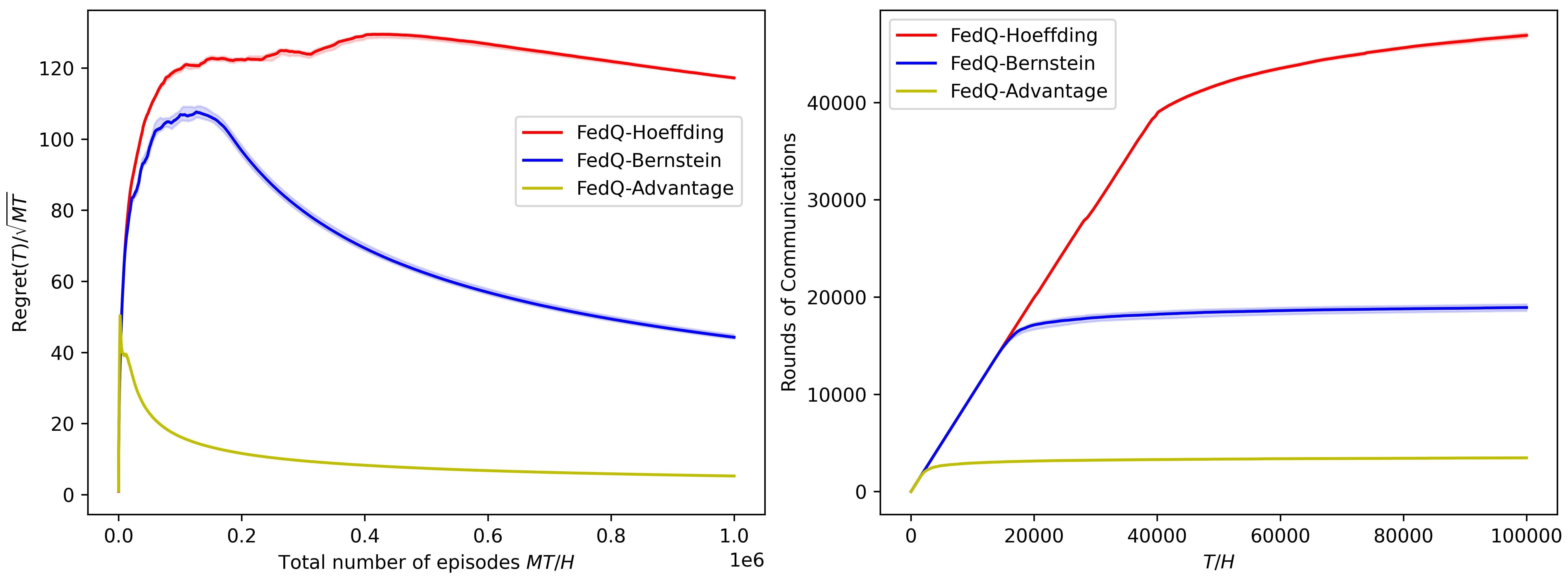
Figure 1: Numerical comparison of regrets and communication costs.

Next, we explain the results. The left panel plots $\mbox{Regret}(T)/\sqrt{MT}$ versus $MT/H$, the total number of episodes for all agents. We see that FedQ-Advantage enjoys lower regret compared to FedQ-Hoeffding and FedQ-Bernstein. The right panel tracks the number of communication rounds throughout the learning process. All three federated algorithms show a sublinear pattern when $T$ is large, and FedQ-Advantage requires the fewest communication rounds. Since the communication cost for one synchronization is $O(MHS)$ for each of the three algorithms, FedQ-Advantage enjoys the least communication cost. These numerical results are consistent with our theoretical results in Table 1. We also provide numerical experiments regarding the multi-agent speedup for FedQ-Advantage in Appendix B.

6 Conclusion

This paper develops the model-free FRL algorithm FedQ-Advantage with provably almost optimal regret and logarithmic communication cost. Specifically, it achieves the regret of $\tilde{O}(\sqrt{H^{2}SAMT})$ with the communication cost $O(M^{2}H^{3}S^{2}A\log(H)\log T)$, reaching the information bound up to a logarithmic factor and near-linear regret speedup compared to its single-agent counterpart when the time horizon is sufficiently large. Technically, our algorithm uses the UCB and reference-advantage decomposition and designs separate mechanisms for synchronization and policy switching, which can find broader applications for other RL problems.

Organization of the appendix. In the appendix, Section A provides related works. Section B provides more numerical results. Section C shows a more general framework for asynchronization. Section D provides basic facts of FedQ-Advantage and a lemma of concentration inequalities for our regret analysis. Section E provides the proof of Theorem 4.1 (regret). Section F provides the proof of Theorem F (communication cost).

For readers interested in technical details, we recommend learning about Lemma D.1 on basic facts for FedQ-Advantage first. After that, for the proof of Theorem 4.1 (regret), readers can directly start on Section E and refer to technical lemmas in Section D when meeting a reference. For the proof of Theorem 4.2 (communication cost), readers can just focus on Section F.

Appendix A Related works

Single-agent episodic MDPs. There are mainly two types of algorithms for reinforcement learning: model-based and model-free learning. Model-based algorithms learn a model from past experience and make decisions based on this model, while model-free algorithms only maintain a group of value functions and take the induced optimal actions. Due to these differences, model-free algorithms are usually more space-efficient and time-efficient compared to model-based algorithms. However, model-based algorithms may achieve better learning performance by leveraging the learned model.

Next, we discuss the literature on model-based and model-free algorithms for single-agent episodic MDPs. [18], [19], [17], [20], [21], [22], [23],[24],[25] and [9] worked on model-based algorithms. Notably, [9] provided an algorithm that achieves a regret of $\tilde{O}\left(\min\{\sqrt{SAH^{2}T},T\}\right)$, which matches the information lower bound. [8], [26], [11], [12] and [27] work on model-free algorithms. The latter three have introduced algorithms that achieve minimax regret of $\tilde{O}\left(\sqrt{SAH^{2}T}\right)$.

Variance reduction in RL. The reference-advantage decomposition used in [11] and [12] is a technique of variance reduction that was originally proposed for finite-sum stochastic optimization (see e.g. [28, 29, 30]). Later on, model-free RL algorithms also used variance reduction to improve the sample efficiency. For example, it was used in learning with generative models [31, 32, 33], policy evaluation [34, 35, 36, 37], offline RL [38, 39], and Q-Learning [40, 11, 12, 41].

Federated and distributed RL. Existing literature on federated and distributed RL algorithms highlights various aspects. [42],[13], and [5] focused on linear speed up. [43] proposed a parallel RL algorithm with low communication cost. [5] and [14] discussed the improved covering power of heterogeneity. [4], [44], and [3] worked on robustness. Particularly, [3] proposed algorithms in both offline and online settings, obtaining near-optimal sample complexities and achieving superior robustness guarantees.

In addition, several works have investigated federated Q-learning algorithms in different settings, including [45], [46], [47], [48], [5], and [14]. The convergence of decentralized temporal difference algorithms has been analyzed by [49], [50], [51], [52], [53], [54], [55], and [56]. Communication-efficient policy gradient algorithms have been studied by [4] and [57]. The convergence of distributed actor-critic algorithms has been analyzed by [58], [59], and [60]. Federated actor-learner architectures have been explored by [61], [62], and [63]. Distributed inverse reinforcement learning has been examined by [64] and [65].

RL with low switching cost and batched RL. Research in RL with low-switching cost aims to minimize the number of policy switches while maintaining comparable regret bounds to fully adaptive counterparts, and it can be applied to federated RL. In batched RL (e.g., [66], [67]), the agent sets the number of batches and the length of each batch upfront, implementing an unchanged policy in a batch and aiming for fewer batches and lower regret. [10] first introduced the problem of RL with low-switching cost and proposed a $Q$-learning algorithm with lazy updates, achieving $\tilde{O}(SAH^{3}\log T)$ switching costs. This work was advanced by [11], which improved the regret upper bound and the switching cost. Additionally, [68] studied RL under the adaptivity constraint. Recently, [16] proposed a model-based algorithm with $\tilde{O}(\log\log T)$ switching costs. [15] proposed a batched RL algorithm that is well-suited for the federated setting.

Appendix B Numerical experiments on multi-agent speedup

In this section, we provide experiments on the multi-agent speedup of FedQ-Advantage under the same experimental setting as Section 5. Figure 2 reports $\mbox{R}(T)/\sqrt{T}$ versus $T/H$ based on the 10 sample trajectories for FedQ-Advantage and UCB-A. Here, $R(T)=\mbox{Regret}(T)/M$. UCB-A is our single-agent counterpart from [11], and we show the experimental results for both $10^{5}$ episodes for the single-agent experiment and $10^{6}$ episodes, representing the situation where a single agent generates all episodes for FedQ-Advantage under a high communication cost. When showing $R(T)$ for UCB-A with $10^{6}$ episodes, we pretend that $M=10$ and the total number of episodes is $10^{5}$ so that the three situations are comparable. We find that FedQ-Advantage shows a multi-agent speedup compared to UCB-A with $10^{5}$ episodes. However, it exhibits larger regret compared to UCB-A with $10^{6}$ episodes, which results from the multi-agent burn-in cost discussed in Section 4.

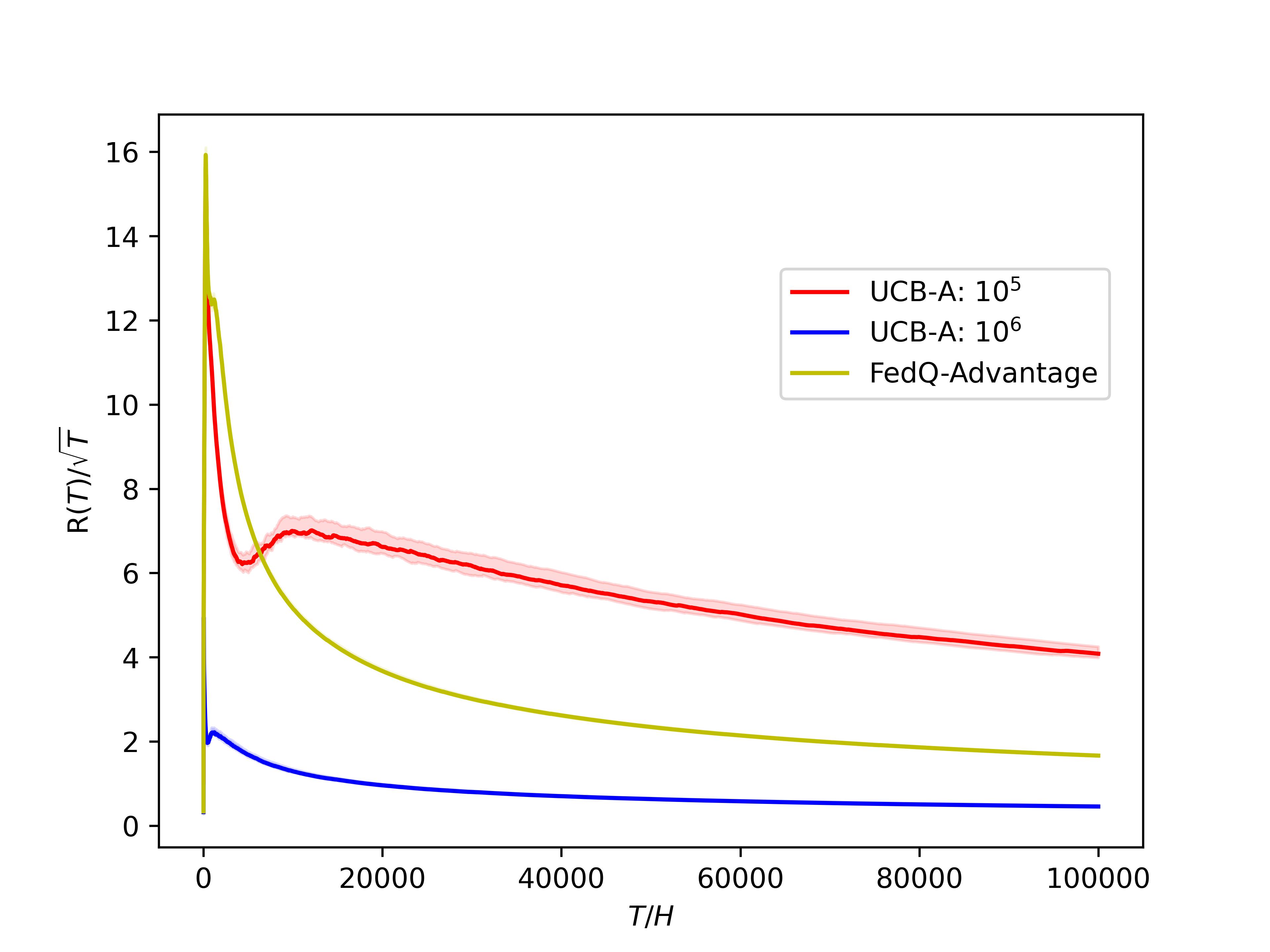
Figure 2: Multi-agent speedup

Appendix C Robustness against asynchronization

In this section, we discuss a more general situation for Algorithms 1 and 2, where agent $m$ generates $n^{m,k}$ episodes during round $k$. We no longer assume that $n^{m,k}$ has the same value $n^{k}$ for different clients. The difference can be caused by latency (the time gap between an agent sending an abortion signal and other agents receiving the signal) and asynchronization (the heterogeneity among clients on the computation speed and process of collecting trajectories). In this case, denoting $K$ as the number of rounds in FedQ-Advantage, the total number of samples generated by all the clients is

$$\hat{T}=H\sum_{k=1}^{K}\sum_{m=1}^{M}n^{m,k}.$$

Thus, we generalize the notation $T=\hat{T}/M$, which characterizes the mean number of samples generated by an agent. Accordingly, the definition of $\mbox{Regret}(T)$ can be generalized as

$$\mbox{Regret}(T)=\sum_{k=1}^{K}\sum_{m=1}^{M}\sum_{j=1}^{n^{m,k}}V_{1}^{\star}(s_{1}^{m,k,j})-V_{1}^{\pi^{k}}(s_{1}^{m,k,j}).$$

We note that Algorithms 1 and 2 naturally accommodate such asynchronicity. Later on, when we provide the proof of Theorems 4.1 and 4.2 and associated intermediate conclusions in Appendices D, E and 4.2, we adopt the general notation $n^{m,k}$.

Appendix D Basic facts and concentration inequalities

In this section, we provide some basic facts and lemmas of concentration inequalities for FedQ-Advantage. For any triple $(s,a,h)\in\mathcal{S}\times\mathcal{A}\times[H]$, we let $Y_{h}^{t}(s,a)=\sum_{m,k:k\leq K}n_{h}^{m,k}\mathbb{I}[t_{h}^{k}\leq t]$ be the number of visits to $(s,a,h)$ up to and including stage $t$ and $y_{h}^{t}(s,a)=\sum_{m,k:k\leq K}n_{h}^{m,k}\mathbb{I}[t_{h}^{k}=t]$ be the visiting number in stage $t$. Here, we have that $Y_{h}^{0}=y_{h}^{0}=0,N_{h}^{k}=Y_{h}^{t_{h}^{k}-1},n_{h}^{k}=y_{h}^{t_{h}^{k}-1}$. We also denote $T_{h}(s,a)=t_{h}^{K}(s,a)$ as the total number of stages for $(s,a,h)$. Here, we emphasize that the stage renewal condition might not be triggered in FedQ-Advantage for stage $T_{h}(s,a)$.

Next, we assign an order to the visits of any $(s,a,h)$. Let $L_{i}(s,a,h)$ denote the $i$-th visit to $(s,a,h)$ in FedQ-Advantage for $i\in\mathbb{N}_{+}$, and $(k_{L_{i}}(s,a,h),m_{L_{i}}(s,a,h),j_{L_{i}}(s,a,h))$ be the corresponding (round, agent, episode) index of the $i$-th visit. Similarly, let $l_{i}(s,a,h,k),i\in[n_{h}^{k}(s,a)]$ denote the $i$-th visit to $(s,a,h)$ during the stage $t_{h}^{k}(s,a)-1$, and $(k_{l_{i}}(s,a,h,k),m_{l_{i}}(s,a,h,k),j_{l_{i}}(s,a,h,k))$ be the corresponding (round, agent, episode) index of the $i$-th visit $l_{i}(s,a,h,k)$. The indices follow the chronological order of the visits. Specifically, under the synchronization assumption $n^{m,k}=n^{k},\forall m\in[M]$, a viable order can be determined by the “round index first, episode index second, agent index third” rule. When $(s,a,h,k)$ is clear from the context, we use $L_{i},l_{i},(k,m,j)_{L_{i}},(k,m,j)_{l_{i}}$ for simplicity.

Next, we provide Lemma D.1 on some basic relationships for quantities in FedQ-Advantage.

Lemma D.1.

For any $(s,a,h,k)\in\mathcal{S}\times\mathcal{A}\times[H]\times[K]$, the following relationships hold for FedQ-Advantage.

• $T_{0}\leq\hat{T}$.

• $n_{h}^{m,k}(s,a)\leq c_{h}^{k}(s,a),\ \forall m\in[M]$. In addition, $\forall k\in[K]$, there exists $(s,a,h,m)\in\mathcal{S}\times\mathcal{A}\times[H]\times[M]$ such that $n_{h}^{m,k}(s,a)=c_{h}^{k}(s,a)$.

• If $T_{h}(s,a)\geq 2$, we have $MH\leq Y_{h}^{1}(s,a)\leq MH+M$.

• If $n_{h}^{k}(s,a)>0$, we have that $\hat{n}_{h}^{k+1}(s,a)\leq(1+2/H)n_{h}^{k}(s,a)$, $\forall k\in[K]$.

• $1+\frac{1}{H}\leq\frac{y_{h}^{t+1}(s,a)}{y_{h}^{t}(s,a)}\leq 1+\frac{2}{H},\forall t\in[1,T_{h}(s,a)-2],t\in\mathbb{N}.$ In addition, $0\leq\frac{y_{h}^{T_{h}}(s,a)}{y_{h}^{T_{h}-1}(s,a)}\leq 1+\frac{2}{H}.$

• $1\leq\frac{Y_{h}^{t+1}(s,a)}{Y_{h}^{t}(s,a)}\leq 2+\frac{2}{H}\leq 4,\forall t\in[T_{h}(s,a)-1].$

• The following relationships hold.

  $$\frac{Y_{h}^{t}(s,a)}{y_{h}^{t}(s,a)}\leq 2H,\forall t\in[T_{h}(s,a)-1].$$ (9)

  $$\sqrt{y_{h}^{t}(s,a)}\leq 3\sqrt{H}\left(\sqrt{Y_{h}^{t}(s,a)}-\sqrt{Y_{h}^{t-1}(s,a)}\right),\forall t\in[T_{h}(s,a)-1].$$ (10)

  $$\frac{Y_{h}^{t}(s,a)}{y_{h}^{t}(s,a)}\geq\frac{H}{4},\forall t\in[H,T_{h}(s,a)],t\in\mathbb{N}.$$ (11)

• $\sum_{s,a,h}y_{h}^{T_{h}(s,a)-1}(s,a)\leq 9MSAH(H+1)+\frac{4T_{0}}{H}$. $\sum_{s,a,h}y_{h}^{T_{h}(s,a)}(s,a)\leq 9MSAH(H+1)+\frac{4T_{0}}{H}$.

• Denote $T_{1}=(2+\frac{2}{H})T_{0}+MSAH(H+1)$, we have

  $$\hat{T}\leq T_{1}\leq(2+\frac{2}{H})\hat{T}+MSAH(H+1).$$

• $Q_{h}^{k+1}(s,a)\leq Q_{h}^{k}(s,a),V_{h}^{k+1}(s)\leq V_{h}^{k}(s),V_{h}^{ref,k+1}(s)\leq V_{h}^{ref,k}(s)$, $\forall(s,a,h,k)\in\mathcal{S}\times\mathcal{A}\times[H]\times[K-1]$.

Here, we use $\sum_{s,a}$ as a simplified notation for $\sum_{s\in\mathcal{S}}\sum_{a\in\mathcal{A}}$ and $\sum_{s,a,h}$ as a simplified notation for $\sum_{s\in\mathcal{S}}\sum_{a\in\mathcal{A}}\sum_{h=1}^{H}$. $T_{h}$ is the simplified notation of $T_{h}(s,a).$ Those simplifications will also be used later.

Proof of Lemma D.1.

1. This relationship holds from the stopping condition of the loop (line 2) in Algorithm 1.

2. From the triggering condition for terminating the exploration in a round (line 4 in Algorithm 2), we can prove the relationship.

3. Since $T_{h}(s,a)\geq 2$, there exists a round $k$ satisfying $t_{h}^{k}(s,a)=1$ and $t_{h}^{k+1}(s,a)=2$. Then according to (4), we have $Y_{h}^{1}(s,a)=\hat{n}_{h}^{k+1}(s,a)\geq MH$. Meanwhile, according to (b), we have:

   $$Y_{h}^{1}(s,a) =\hat{n}_{h}^{k+1}(s,a)=\tilde{n}_{h}^{k}(s,a)+\sum_{m=1}^{M}n_{h}^{m,k}(s,a)$$

   $$\leq\tilde{n}_{h}^{k}(s,a)+Mc_{h}^{k}(s,a)\leq\tilde{n}_{h}^{k}(s,a)+M.$$

   Since round $k$ is in stage 1, we know stage 1 is not renewed before the start of round $k$. Then according to (4) and the definition of $\tilde{n}_{h}^{k}(s,a)$, we have $\tilde{n}_{h}^{k}(s,a)\leq MH$ and $Y_{h}^{1}(s,a)\leq\tilde{n}_{h}^{k}(s,a)+M=MH+M$.

4. Since round $k$ is in the stage $t_{h}^{k}$, we know stage $t_{h}^{k}$ is not renewed before the start of round $k$. Then according to (4) and the definition of $\tilde{n}_{h}^{k}(s,a)$, we have $\tilde{n}_{h}^{k}(s,a)\leq(1+1/H)n_{h}^{k}(s,a)$.

   If $0\leq\tilde{n}_{h}^{k}(s,a)\leq(1-\frac{1}{H})n_{h}^{k}(s,a)$, then according to (2) we have:

   $$\hat{n}_{h}^{k+1}(s,a)\leq\tilde{n}_{h}^{k}(s,a)+Mc_{h}^{k}(s,a) \leq\tilde{n}_{h}^{k}(s,a)+M\left(\frac{n_{h}^{k}(s,a)-\tilde{n}_{h}^{k}(s,a)}{M}+1\right)$$

   $$=n_{h}^{k}(s,a)+M.$$

   Since $n_{h}^{k}(s,a)>0$, we know $t_{h}^{k}(s,a)>1$ and then $n_{h}^{k}(s,a)\geq Y_{h}^{1}(s,a)\geq MH$. Therefore, $\hat{n}_{h}^{k+1}(s,a)\leq n_{h}^{k}(s,a)+M\leq(1+\frac{2}{H})n_{h}^{k}(s,a)$.

   If $(1-1/H)n_{h}^{k}(s,a)<\tilde{n}_{h}^{k}(s,a)\leq(1+1/H)n_{h}^{k}(s,a)$, then according to (2) we have:

   $$\hat{n}_{h}^{k+1}(s,a)\leq\tilde{n}_{h}^{k}(s,a)+Mc_{h}^{k}(s,a)\leq\tilde{n}_{h}^{k}(s,a)+M\cdot\frac{1}{MH}n_{h}^{k}(s,a)\leq(1+\frac{2}{H})n_{h}^{k}(s,a).$$

   Therefore, $\tilde{n}_{h}^{k}(s,a)\leq(1+\frac{2}{H})n_{h}^{k}(s,a)$.

5. For $t\leq T_{h}(s,a)-2$, there exists a round $k$ satisfying $t_{h}^{k}(s,a)=t+1$ and $t_{h}^{k+1}(s,a)=t+2$. Then according to (2), we have $y_{h}^{t+1}(s,a)=\hat{n}_{h}^{k+1}(s,a)\geq(1+1/H)n_{h}^{k}(s,a)=(1+1/H)y_{h}^{t}(s,a)$. Moreover, according to (d), we have $y_{h}^{t+1}(s,a)=\hat{n}_{h}^{k+1}(s,a)\leq(1+2/H)n_{h}^{k}(s,a)=(1+2/H)y_{h}^{t}(s,a)$.

   For $t=T_{h}(s,a)-1$, we have $y_{h}^{T_{h}}(s,a)=\hat{n}_{h}^{K+1}(s,a)\leq(1+2/H)n_{h}^{K}(s,a)=(1+2/H)y_{h}^{T_{h}-1}(s,a)$.

6. According to (e), for $t\leq T_{h}(s,a)-1$ we have $y_{h}^{t+1}(s,a)\leq(1+2/H)y_{h}^{t}(s,a)$. Then:

   $$1\leq\frac{Y_{h}^{t+1}(s,a)}{Y_{h}^{t}(s,a)}=1+\frac{y_{h}^{t+1}(s,a)}{Y_{h}^{t}(s,a)}\leq 1+\frac{(1+\frac{2}{H})y_{h}^{t}(s,a)}{Y_{h}^{t}(s,a)}\leq 2+\frac{2}{H}\leq 4.$$

7. We will use the mathematical induction to prove the (9).

   For $t=1$,

   $$\frac{Y_{h}^{1}(s,a)}{y_{h}^{1}(s,a)}=1\leq 2H.$$

   If $\frac{Y_{h}^{t-1}(s,a)}{y_{h}^{t-1}(s,a)}\leq 2H$, then for $t$ ($2\leq t\leq T_{h}(s,a)-1$), according to (e), we have $y_{h}^{t}(s,a)\geq(1+1/H)y_{h}^{t-1}(s,a)$. Then:

   $$\frac{Y_{h}^{t}(s,a)}{y_{h}^{t}(s,a)}=1+\frac{Y_{h}^{t-1}(s,a)}{y_{h}^{t}(s,a)}\leq 1+\frac{Y_{h}^{t-1}(s,a)}{(1+\frac{1}{H})y_{h}^{t-1}(s,a)}\leq 1+\frac{2H}{1+\frac{1}{H}}\leq 2H.$$

   Therefore, we finish the proof of the (9).

   For (10), we have:

   $$3\sqrt{H}\left(\sqrt{Y_{h}^{t}(s,a)}-\sqrt{Y_{h}^{t-1}(s,a)}\right)$$

   $$=\sqrt{y_{h}^{t}(s,a)}\cdot 3\sqrt{H}\left(\sqrt{\frac{Y_{h}^{t}(s,a)}{y_{h}^{t}(s,a)}}-\sqrt{\frac{Y_{h}^{t}(s,a)}{y_{h}^{t}(s,a)}-1}\right)$$

   $$=\sqrt{y_{h}^{t}(s,a)}\cdot 3\sqrt{H}\frac{1}{\sqrt{\frac{Y_{h}^{t}(s,a)}{y_{h}^{t}(s,a)}}+\sqrt{\frac{Y_{h}^{t}(s,a)}{y_{h}^{t}(s,a)}-1}}$$

   $$\geq\sqrt{y_{h}^{t}(s,a)}\cdot 3\sqrt{H}\frac{1}{\sqrt{2H}+\sqrt{2H-1}}\geq\sqrt{y_{h}^{t}(s,a)}.$$

   The last but one inequality is because $\frac{Y_{h}^{t}(s,a)}{y_{h}^{t}(s,a)}\leq 2H$ according to (9).

   For (11), according to (e), we have $y_{h}^{t}(s,a)\leq(1+2/H)^{h-1}y_{h}^{t-h+1}(s,a)$ for any $h\in[H]$. Then:

   $$\frac{Y_{h}^{t}(s,a)}{y_{h}^{t}(s,a)}\geq\frac{\sum_{h=1}^{H}y_{h}^{t-h+1}(s,a)}{y_{h}^{t}(s,a)} \geq\frac{\sum_{h=1}^{H}(1+\frac{2}{H})^{1-h}y_{h}^{t}(s,a)}{y_{h}^{t}(s,a)}$$

   $$=\frac{H}{2}(1+\frac{2}{H})(1-(1+\frac{2}{H})^{-H}).$$

   Because $(1+\frac{2}{H})^{H}$ is increasing in $H$, we have $(1+\frac{2}{H})^{H}\geq 3$ and $1-(1+\frac{2}{H})^{-H}\geq\frac{2}{3}$. Therefore,

   $$\frac{Y_{h}^{t}(s,a)}{y_{h}^{t}(s,a)}\geq\frac{H}{2}(1+\frac{2}{H})(1-(1+\frac{2}{H})^{-H})\geq\frac{H}{4}.$$

   We finish the proof of (g).

8. $$\sum_{s,a,h}y_{h}^{T_{h}(s,a)-1}(s,a) =\sum_{s,a,h}y_{h}^{T_{h}-1}(s,a)\mathbb{I}[T_{h}(s,a)<H+1]$$

   $$\quad+\sum_{s,a,h}y_{h}^{T_{h}-1}(s,a)\mathbb{I}[T_{h}(s,a)\geq H+1]$$

   Because of (e), we have:

   $$y_{h}^{T_{h}-1}(s,a)\mathbb{I}[T_{h}(s,a)<H+1] \leq(1+\frac{2}{H})^{T_{h}-1}y_{h}^{1}(s,a)\mathbb{I}[T_{h}(s,a)<H+1]$$

   $$\leq(1+\frac{2}{H})^{H}(MH+M).$$

   The last inequality is because $y_{h}^{1}(s,a)=Y_{h}^{1}(s,a)\leq MH+M$ according to (c). Moreover, according to (11), we have

   $$\sum_{s,a,h}y_{h}^{T_{h}-1}(s,a)\mathbb{I}[T_{h}(s,a)\geq H+1]\leq\sum_{s,a,h}\frac{4}{H}Y_{h}^{T_{h}-1}(s,a)\mathbb{I}[T_{h}(s,a)\geq H+1]\leq\frac{4T_{0}}{H}.$$

   The last inequality holds because $\sum_{s,a,h}Y_{h}^{T_{h}-1}(s,a)\leq T_{0}$ according to the algorithm. Therefore, we have

   $$\sum_{s,a,h}y_{h}^{T_{h}(s,a)-1}(s,a)\leq\sum_{s,a,h}(1+\frac{2}{H})^{H}(MH+M)+\frac{4T_{0}}{H}\leq 9MSAH(H+1)+\frac{4T_{0}}{H}.$$

   Similarly, we have:

   $$\sum_{s,a,h}y_{h}^{T_{h}(s,a)}(s,a)$$

   $$=\sum_{s,a,h}y_{h}^{T_{h}}(s,a)\mathbb{I}[T_{h}(s,a)<H+1]+\sum_{s,a,h}y_{h}^{T_{h}-1}(s,a)\mathbb{I}[T_{h}(s,a)\geq H+1]$$

   $$\leq(1+\frac{2}{H})^{T_{h}-1}y_{h}^{1}(s,a)\mathbb{I}[T_{h}(s,a)<H+1]+\sum_{s,a,h}\frac{4}{H}Y_{h}^{T_{h}-1}(s,a)\mathbb{I}[T_{h}(s,a)\geq H+1]$$

   $$\leq 9MSAH(H+1)+\frac{4T_{0}}{H}.$$

9. First, according to (f), we have:

   $$Y_{h}^{T_{h}}(s,a) \leq Y_{h}^{1}(s,a)\mathbb{I}[T_{h}(s,a)=1]+(2+\frac{2}{H})Y_{h}^{T_{h}-1}(s,a)\mathbb{I}[T_{h}(s,a)>1]$$

   $$\leq(2+\frac{2}{H})Y_{h}^{T_{h}-1}(x,a)+MH+M.$$

   The last inequality is because of (c). Then we have:

   $$\hat{T}=\sum_{s,a,h}Y_{h}^{T_{h}}(s,a) \leq\sum_{s,a,h}\left((2+\frac{2}{H})Y_{h}^{T_{h}-1}(s,a)+MH+M\right)$$

   $$\leq(2+\frac{2}{H})T_{0}+MSAH(H+1).$$

   The last inequality is because of $\sum_{s,a,h}Y_{h}^{T_{h}-1}(s,a)\leq T_{0}$ according to the algorithm. Because $T_{0}\leq\hat{T}$ from (a), we have:

   $$\hat{T}\leq T_{1}\leq(2+\frac{2}{H})\hat{T}+MSAH(H+1).$$

10. According to (5), we know $Q_{h}^{k}(s,a)$ is non-increasing with respect to $k$. Then based on the update rule (7) for $V_{h}^{k}(s,a)$ and the update rule (8) for $V_{h}^{ref,k}(s,a)$, we find that they are also non-increasing with respect to $k$.

∎

Next, we provide Lemma D.2 that discusses the weighted sum of all the steps.

Lemma D.2.

For any non-negative weight sequence $\left\{\omega_{h}(s,a)\right\}_{s,a,h}$ and any $\alpha\in(0,1)$, it holds that

$$\sum_{h=1}^{H}\sum_{k,m,j}\frac{\omega_{h}(s_{h}^{k,m,j},a_{h}^{k,m,j})}{N_{h}^{k}(s_{h}^{k,m,j},a_{h}^{k,m,j})^{\alpha}}\mathbb{I}\left[t_{h}^{k,m,j}>1\right]\leq\frac{4^{\alpha}}{1-\alpha}\sum_{s,a,h}\omega_{h}(s,a)Y_{h}^{T_{h}}(s,a)^{1-\alpha},$$

and

$$\sum_{h=1}^{H}\sum_{k,m,j}\frac{\omega_{h}(s_{h}^{k,m,j},a_{h}^{k,m,j})}{n_{h}^{k}(s_{h}^{k,m,j},a_{h}^{k,m,j})^{\alpha}}\mathbb{I}\left[t_{h}^{k,m,j}>1\right]\leq\frac{(8H)^{\alpha}}{1-\alpha}\sum_{s,a,h}\omega_{h}(s,a)Y_{h}^{T_{h}}(s,a)^{1-\alpha}.$$

For $\alpha=1$, it holds that

$$\sum_{h=1}^{H}\sum_{k,m,j}\frac{\omega_{h}(s_{h}^{k,m,j},a_{h}^{k,m,j})}{N_{h}^{k}(s_{h}^{k,m,j},a_{h}^{k,m,j})}\mathbb{I}\left[t_{h}^{k,m,j}>1\right]\leq 4\sum_{s,a,h}\omega_{h}(s,a)\log(Y_{h}^{T_{h}}(s,a)),$$

and

$$\sum_{h=1}^{H}\sum_{k,m,j}\frac{\omega_{h}(s_{h}^{k,m,j},a_{h}^{k,m,j})}{n_{h}^{k}(s_{h}^{k,m,j},a_{h}^{k,m,j})}\mathbb{I}\left[t_{h}^{k,m,j}>1\right]\leq 8H\sum_{s,a,h}\omega_{h}(s,a)\log(Y_{h}^{T_{h}}(s,a)).$$

Here, $t_{h}^{k,m,j}=t_{h}^{k}(s_{h}^{k,m,j},a_{h}^{k,m,j})$.

Proof of Lemma D.2.

According to (9), for any $(s_{h}^{k,m,j},a_{h}^{k,m,j},h)\in\mathcal{S}\times\mathcal{A}\times[H]$ and $t_{h}^{k,m,j}>1$,

$$\frac{N_{h}^{k}(s_{h}^{k,m,j},a_{h}^{k,m,j})}{n_{h}^{k}(s_{h}^{k,m,j},a_{h}^{k,m,j})}=\frac{Y_{h}^{t_{h}^{k,m,j}-1}(s_{h}^{k,m,j},a_{h}^{k,m,j})}{y_{h}^{t_{h}^{k,m,j}-1}(s_{h}^{k,m,j},a_{h}^{k,m,j})}\leq 2H.$$

Therefore, we only need to prove the first and the third inequalities.

We first provide two conclusions. For $1\leq x\leq 4$ and $0<\alpha<1$, it holds:

$$x^{1-\alpha}-1\geq(1-\alpha)(x-1)x^{-\alpha}\geq 4^{-\alpha}(1-\alpha)(x-1)$$ (12)

$$\log(x)\geq\frac{x-1}{x}\geq\frac{x-1}{4}.$$ (13)

Next, we go back to the proof. For any $(s,a,h)\in\mathcal{S}\times\mathcal{A}\times[H]$ and $2\leq t\leq T_{h}(s,a)$, let $x=\frac{Y_{h}^{t}(s,a)}{Y_{h}^{t-1}(s,a)}$. According to (f) in Lemma D.1, we have $1\leq x\leq 4$. Using (12), and (13), then it holds:

$$Y_{h}^{t}(s,a)^{1-\alpha}-{Y_{h}^{t-1}(s,a)}^{1-\alpha}\geq 4^{-\alpha}(1-\alpha)\frac{y_{h}^{t}(s,a)}{Y_{h}^{t-1}(s,a)^{\alpha}},$$ (14)

and

$$\log(Y_{h}^{t}(s,a))-\log(Y_{h}^{t-1}(s,a))\geq\frac{y_{h}^{t}(s,a)}{4Y_{h}^{t-1}(s,a)}.$$ (15)

Now,

$$\sum_{h=1}^{H}\sum_{k,m,j}\frac{\omega_{h}(s_{h}^{k,m,j},a_{h}^{k,m,j})}{N_{h}^{k}(s_{h}^{k,m,j},a_{h}^{k,m,j})^{\alpha}}\mathbb{I}\left[t_{h}^{k,m,j}>1\right]$$

$$=\sum_{h=1}^{H}\sum_{k,m,j}\frac{\omega_{h}(s_{h}^{k,m,j},a_{h}^{k,m,j})}{N_{h}^{k}(s_{h}^{k,m,j},a_{h}^{k,m,j})^{\alpha}}\mathbb{I}\left[t_{h}^{k,m,j}>1\right]\left(\sum_{s,a}\mathbb{I}\left[(s_{h}^{k,m,j},a_{h}^{k,m,j})=(s,a)\right]\right)$$

$$=\sum_{s,a,h}\sum_{k,m,j}\frac{\omega_{h}(s,a)}{N_{h}^{k}(s,a)^{\alpha}}\mathbb{I}\left[t_{h}^{k}(s,a)>1\right]\mathbb{I}\left[(s_{h}^{k,m,j},a_{h}^{k,m,j})=(s,a)\right]$$

$$=\sum_{s,a,h}\sum_{k,m,j}\frac{\omega_{h}(s,a)}{N_{h}^{k}(s,a)^{\alpha}}\mathbb{I}\left[(s_{h}^{k,m,j},a_{h}^{k,m,j})=(s,a)\right]\left(\sum_{t=2}^{T_{h}}\mathbb{I}\left[t_{h}^{k}(s,a)=t\right]\right)$$

$$=\sum_{s,a,h}\sum_{t=2}^{T_{h}}\frac{\omega_{h}(s,a)}{N_{h}^{k}(s,a)^{\alpha}}\sum_{k,m,j}\mathbb{I}\left[(s_{h}^{k,m,j},a_{h}^{k,m,j})=(s,a),t_{h}^{k}(s,a)=t\right]$$

In the last equality, $\mathbb{I}[(s_{h}^{k,m,j},a_{h}^{k,m,j})=(s,a),t_{h}^{k}(s,a)=t]=1$ if and only if $(s_{h}^{k,m,j},a_{h}^{k,m,j})=(s,a)$ and $k$ in stage $t$ of $(s,a,h)$, so $\sum_{k,m,j}\mathbb{I}[(s_{h}^{k,m,j},a_{h}^{k,m,j})=(s,a),t_{h}^{k}(s,a)=t]=y_{h}^{t}(s,a)$. In this case, $N_{h}^{k}(s,a)=Y_{h}^{t-1}(s,a)$ and then we have :

$$\sum_{h=1}^{H}\sum_{k,m,j}\frac{\omega_{h}(s_{h}^{k,m,j},a_{h}^{k,m,j})}{N_{h}^{k}(s_{h}^{k,m,j},a_{h}^{k,m,j})^{\alpha}}\mathbb{I}\left[t_{h}^{k,m,j}>1\right]=\sum_{s,a,h}\sum_{t=2}^{T_{h}}\frac{\omega_{h}(s,a)y_{h}^{t}(s,a)}{Y_{h}^{t-1}(s,a)^{\alpha}}.$$ (16)

Summing (14) for $2\leq t\leq T_{h}(s,a)$, for any $0<\alpha<1$, we have:

$$\sum_{t=2}^{T_{h}}\frac{y_{h}^{t}(s,a)}{Y_{h}^{t-1}(s,a)^{\alpha}}\leq\frac{4^{\alpha}}{1-\alpha}\sum_{t=2}^{T_{h}}(Y_{h}^{t}(s,a)^{1-\alpha}-{Y_{h}^{t-1}(s,a)}^{1-\alpha})\leq\frac{4^{\alpha}}{1-\alpha}Y_{h}^{T_{h}}(s,a)^{1-\alpha}$$ (17)

Combining (16) and (17), we can finish the proof of the first inequality.

In (16), let $\alpha=1$, we have:

$$\sum_{h=1}^{H}\sum_{k,m,j}\frac{\omega_{h}(s_{h}^{k,m,j},a_{h}^{k,m,j})}{N_{h}^{k}(s_{h}^{k,m,j},a_{h}^{k,m,j})}\mathbb{I}\left[t_{h}^{k,m,j}>1\right]=\sum_{s,a,h}\omega_{h}(s,a)\sum_{t=1}^{T_{h}}\frac{y_{h}^{t}(s,a)}{Y_{h}^{t-1}(s,a)}$$ (18)

Summing (15) for $2\leq t\leq T_{h}(s,a)$ , we have:

$$\sum_{t=2}^{T_{h}}\frac{y_{h}^{t}(s,a)}{Y_{h}^{t-1}(s,a)}\leq 4\sum_{t=2}^{T_{h}}\left(\log(Y_{h}^{t}(s,a))-\log(Y_{h}^{t-1}(s,a))\right)\leq 4\log(Y_{h}^{T_{h}}(s,a))$$ (19)

Combining (18) with (19), we finish the proof of the third inequality. Then we finish the proof. ∎

Next, we provide auxiliary lemmas.

Lemma D.3.

(Azuma-Hoeffding Inequality) Suppose $\left\{X_{k}\right\}_{k=0}^{\infty}$ is a martingale and $|X_{k}-X_{k-1}|\leq c_{k}$, $\forall k\in\mathbb{N}_{+}$ almost surely. Then for any positive integers $N$ and any positive real number $\epsilon$, it holds that:

$$\mathbb{P}\left(|X_{N}-X_{0}|\geq\epsilon\right)\leq 2\exp\left(-\frac{\epsilon^{2}}{2\sum_{k=1}^{N}c_{k}^{2}}\right).$$

Lemma D.4.

(Lemma 10 of [11]) Let $\left\{M_{n}\right\}_{n=0}^{\infty}$ be a martingale such that $M_{0}=0$ and $|M_{n}-M_{n-1}|\leq c$. Let $Var_{n}=\sum_{k=1}^{n}\mathbb{E}[(M_{k}-M_{k-1})^{2}|\mathcal{F}_{k-1}]$, where $\mathcal{F}_{k-1}=\sigma(M_{0},M_{1},...,M_{k-1})$. Then for any positive integer $n$ and any $\epsilon,p>0$, we have that:

$$\mathbb{P}\left(|M_{n}|\geq 2\sqrt{\textnormal{Var}_{n}\log(1/p)}+2\sqrt{\epsilon\log(1/p)}+2c\log(1/p)\right)\leq\left(2nc^{2}/\epsilon+2\right)p.$$

At the end of this section, we provide a lemma of concentration inequalities.

Lemma D.5.

Let $\iota=\log(2/p)$ with $p\in(0,1)$. Using $\forall(s,a,h,k)$ as the simplified notation for $\forall(s,a,h,k)\in\mathcal{S}\times\mathcal{A}\times[H]\times[K]$. For any function $f:\mathcal{S}\rightarrow\mathbb{R}$, we denote $\mathbb{V}_{s,a,h}(f)=\mathbb{P}_{s,a,h}f^{2}-(\mathbb{P}_{s,a,h}f)^{2}$. Next, we define the following events.

$$\mathcal{E}_{1}=\left\{\frac{1}{n_{h}^{k}}\left|\sum_{i=1}^{n_{h}^{k}}\left(V_{h+1}^{\star}(s_{h+1}^{(k,m,j)_{l_{i}}})-\mathbb{P}_{s,a,h}V_{h+1}^{\star}\right)\right|\leq\sqrt{\frac{2H^{2}\iota}{n_{h}^{k}}},\forall(s,a,h,k)\right\}.$$

$$\mathcal{E}_{2}=\left\{|\chi_{1}|\leq\frac{2}{N_{h}^{k}}\left(\sqrt{\sum_{i=1}^{N_{h}^{k}}\mathbb{V}_{s,a,h}(V_{h+1}^{ref,k_{L_{i}}})\iota}+\frac{\sqrt{\iota}}{T_{1}}+H\iota\right),\forall(s,a,h,k)\right\},$$

in which $\chi_{1}$ is the abbreviation for

$$\chi_{1}(s,a,h,k)=\frac{1}{N_{h}^{k}(s,a)}\sum_{i=1}^{N_{h}^{k}}\left(\mathbb{P}_{s,a,h}-\mathbbm{1}_{s_{h+1}^{(k,m,j)_{L_{i}}}}\right)V_{h+1}^{ref,k_{L_{i}}}.$$

$$\mathcal{E}_{3}=\left\{\left|\sum_{i=1}^{N_{h}^{k}}\left(\mathbb{P}_{s,a,h}-\mathbbm{1}_{s_{h+1}^{(k,m,j)_{L_{i}}}}\right)V_{h+1}^{ref,k_{L_{i}}}\right|\leq H\sqrt{2N_{h}^{k}(s,a)\iota},\forall(s,a,h,k)\right\}.$$

$$\mathcal{E}_{4}=\left\{\left|\sum_{i=1}^{N_{h}^{k}}\left(\mathbb{P}_{s,a,h}-\mathbbm{1}_{s_{h+1}^{(k,m,j)_{L_{i}}}}\right)(V_{h+1}^{ref,k_{L_{i}}})^{2}\right|\leq H^{2}\sqrt{2N_{h}^{k}(s,a)\iota},\forall(s,a,h,k)\right\}.$$

$$\mathcal{E}_{5}=\left\{|\chi_{2}|\leq\frac{2}{n_{h}^{k}}\left(\sqrt{\sum_{i=1}^{n_{h}^{k}}\mathbb{V}_{s,a,h}(V_{h+1}^{k_{l_{i}}}-V_{h+1}^{ref,k_{l_{i}}})\iota}+\frac{\sqrt{\iota}}{T_{1}}+2H\iota\right),\forall(s,a,h,k)\right\},$$

in which $\chi_{2}$ is the abbreviation for

$$\chi_{2}(s,a,h,k)=\frac{1}{n_{h}^{k}}\sum_{i=1}^{n_{h}^{k}}\left(\mathbb{P}_{s,a,h}-\mathbbm{1}_{s_{h+1}^{(k,m,j)_{l_{i}}}}\right)(V_{h+1}^{k_{l_{i}}}-V_{h+1}^{ref,k_{l_{i}}}).$$

$$\mathcal{E}_{6}=\left\{\left|\sum_{i=1}^{n_{h}^{k}}\left(\mathbb{P}_{s,a,h}-\mathbbm{1}_{s_{h+1}^{(k,m,j)_{l_{i}}}}\right)(V_{h+1}^{k_{l_{i}}}-V_{h+1}^{ref,k_{l_{i}}})\right|\leq 2H\sqrt{2n_{h}^{k}(s,a)\iota},\forall(s,a,h,k)\right\}.$$

$$\mathcal{E}_{7}=\left\{\left|\sum_{i=1}^{n_{h}^{k}}\left(\mathbb{P}_{s,a,h}-\mathbbm{1}_{s_{h+1}^{(k,m,j)_{l_{i}}}}\right)(V_{h+1}^{k_{l_{i}}}-V_{h+1}^{ref,k_{l_{i}}})^{2}\right|\leq 2H^{2}\sqrt{2n_{h}^{k}(s,a)\iota},\forall(s,a,h,k)\right\}.$$

$$\mathcal{E}_{8}=\left\{\left|\sum_{h=1}^{H}\sum_{k,m,j}\left(\mathbb{P}_{s_{h}^{k,m,j},a_{h}^{k,m,j},h}-\mathbbm{1}_{s_{h+1}^{k,m,j}}\right)\lambda_{h+1}^{k}(s_{h+1}^{k,m,j})\right|\leq\sqrt{2T_{1}\iota}\right\}.$$

Here, $\lambda_{h}^{k}(s)=\mathbb{I}[N_{h}^{k}(s)<N_{0}]$ with $N_{h}^{k}(s)=\sum_{a\in\mathcal{A}}N_{h}^{k}(s,a)$. Especially, $\lambda_{H+1}^{k}(s)=0$. $\sum_{k,m,j}$ is the abbreviation of $\sum_{k=1}^{K}\sum_{m=1}^{M}\sum_{j=1}^{n^{m,k}}$. We will also use the abbreviation later.

$$\mathcal{E}_{9}=\left\{\sum_{h=1}^{H}\sum_{k,m,j}(1+\frac{2}{H})^{h}\left(\mathbb{P}_{s_{h}^{k,m,j},a_{h}^{k,m,j},h}-\mathbbm{1}_{s_{h+1}^{k,m,j}}\right)\left(V_{h+1}^{k}-V^{\star}_{h+1}\right)\leq 18H\sqrt{2T_{1}\iota}\right\}$$

$$\mathcal{E}_{10}=\left\{\left|V(s,a,h,t)\right|\leq H\sqrt{2y_{h}^{t}(s,a)\iota},\forall(s,a,h)\text{ and }\forall t\in[T_{h}(s,a)]\right\}.$$

Here,

$$V(s,a,h,t)=\sum_{k,m,j}\left(\mathbb{P}_{s,a,h}-\mathbbm{1}_{s_{h+1}^{k,m,j}}\right)\left(V_{h+1}^{k}-V^{\star}_{h+1}\right)\mathbb{I}\left[(s_{h}^{k,m,j},a_{h}^{k,m,j})=(s,a),t_{h}^{k}(s,a)=t\right].$$

$$\mathcal{E}_{11}=\Bigg{\{} \sum_{h=1}^{H}\sum_{k,m,j}(1+\frac{2}{H})^{h-1}\mathbb{I}\left[t_{h}^{k,m,j}>1\right]\left(\mathbb{P}_{s_{h}^{k,m,j},a_{h}^{k,m,j},h}-\mathbbm{1}_{s_{h+1}^{k,m,j}}\right)\left(V_{h+1}^{\star}-V_{h+1}^{\pi^{k}}\right)\Bigg{.}$$

$$\Bigg{.}\leq 9H\sqrt{2T_{1}\iota}\Bigg{\}}.$$

$$\mathcal{E}_{12}=\left\{\frac{1}{N_{h}^{k}(s,a)}\left|\sum_{i=1}^{N_{h}^{k}(s,a)}\left(\mathbb{P}_{s,a,h}-\mathbbm{1}_{s_{h+1}^{(k,m,j)_{L_{i}}}}\right)\lambda_{h+1}^{k_{L_{i}}}\right|\leq\sqrt{\frac{2\iota}{N_{h}^{k}(s,a)}},\forall(s,a,h,k)\right\}.$$

$$\mathcal{E}_{13}=\left\{\left|\sum_{h=1}^{H}\sum_{k,m,j}\left(\mathbb{P}_{s_{h}^{k,m,j},a_{h}^{k,m,j},h}(V_{h+1}^{\star})-V_{h+1}^{\star}(s_{h+1}^{k,m,j})\right)\right|\leq H\sqrt{2T_{1}\iota}\right\}.$$

$$\mathcal{E}_{14}=\left\{\left|\sum_{h=1}^{H}\sum_{k,m,j}\left(\mathbb{P}_{s_{h}^{k,m,j},a_{h}^{k,m,j},h}(V_{h+1}^{\star})^{2}-V_{h+1}^{\star}(s_{h+1}^{k,m,j})^{2}\right)\right|\leq H^{2}\sqrt{2T_{1}\iota}\right\}.$$

$$\mathcal{E}_{15}=\left\{\left|\frac{1}{N_{h}^{k}(s,a)}\sum_{i=1}^{N_{h}^{k}(s,a)}\left(\mathbb{P}_{s,a,h}-\mathbbm{1}_{s_{h+1}^{(k,m,j)_{L_{i}}}}\right)\left(V_{h+1}^{ref,k_{L_{i}}}-V_{h+1}^{\star}\right)\right|\leq 2H\sqrt{\frac{2\iota}{N_{h}^{k}(s,a)}}.\right\}.$$

Then we have

$$\mathbb{P}(\mathcal{E}_{i})\geq 1-SAT_{1}^{2}/Hp,i\in\{1,6,7,10\},$$

$$\mathbb{P}(\mathcal{E}_{i})\geq 1-SAT_{1}p,i\in\{3,4,12,15\},$$

$$\mathbb{P}(\mathcal{E}_{i})\geq 1-p,i\in\{8,9,11,13,14\},$$

$$\mathbb{P}(\mathcal{E}_{2})\geq 1-SAT_{1}(HT_{1}^{3}+1)p$$

and

$$\mathbb{P}(\mathcal{E}_{5})\geq 1-SAT_{1}^{2}(4HT_{1}^{3}+1)/Hp.$$

Proof of Lemma D.5.

First, we will prove with probability at least $1-SAT_{1}^{2}/Hp$, $\mathcal{E}_{1}$ holds. The sequence $\{V_{h+1}^{\star}(s_{h+1}^{(k,m,j)_{l_{i}}})-\mathbb{P}_{s,a,h}V_{h+1}^{\star}\}_{i\in\mathbb{N}^{+}}$ is a martingale sequence with its absolute values bounded by $H$ . Then according to Azuma-Hoeffding inequality, for any $p\in(0,1)$, with probability at least $1-p$, it holds for given $n_{h}^{k}(s,a)=n\in\mathbb{N}_{+}$ that:

$$\frac{1}{n}\left|\sum_{i=1}^{n}\left(V_{h+1}^{\star}(s_{h+1}^{(k,m,j)_{l_{i}}})-\mathbb{P}_{s,a,h}V_{h+1}^{\star}\right)\right|\leq\sqrt{\frac{2H^{2}\iota}{n}}.$$

For any $k\in[K]$, we have $n_{h}^{k}(s,a)\in[\frac{T_{1}}{H}]$. Considering all the possible combinations $(s,a,h,k)\in\mathcal{S}\times\mathcal{A}\times[H]\times[\frac{T_{1}}{H}]$ and $n_{h}^{k}(s,a)\in[\frac{T_{1}}{H}]$, with probability at least $1-SAT_{1}^{2}/Hp$, it holds simultaneously for all $(s,a,h,k)\in\mathcal{S}\times\mathcal{A}\times[H]\times[K]$ that:

$$\frac{1}{n_{h}^{k}(s,a)}\left|\sum_{i=1}^{n_{h}^{k}}\left(V_{h+1}^{\star}(s_{h+1}^{(k,m,j)_{l_{i}}})-\mathbb{P}_{s,a,h}V_{h+1}^{\star}\right)\right|\leq\sqrt{\frac{2H^{2}\iota}{n_{h}^{k}(s,a)}}.$$

This conclusion also holds for for $\mathcal{E}_{6}$ and $\mathcal{E}_{7}$ as $\{(\mathbb{P}_{s,a,h}-\mathbbm{1}_{s_{h+1}^{(k,m,j)_{l_{i}}}})(V_{h+1}^{k_{l_{i}}}-V_{h+1}^{ref,k_{l_{i}}})\}_{i\in\mathbb{N}^{+}}$ is a martingale sequence with its absolute values bounded by $2H$, and $\{(\mathbb{P}_{s,a,h}-\mathbbm{1}_{s_{h+1}^{(k,m,j)_{l_{i}}}})(V_{h+1}^{k_{l_{i}}}-V_{h+1}^{ref,k_{l_{i}}})^{2}\}_{i\in\mathbb{N}^{+}}$ is a martingale sequence with its absolute values bounded by $2H^{2}$.

Next, we will prove with probability at least $1-SAT_{1}p$, $\mathcal{E}_{3}$ holds. $\{(\mathbb{P}_{s,a,h}-\mathbbm{1}_{s_{h+1}^{(k,m,j)_{L_{i}}}})V_{h+1}^{ref,k_{L_{i}}}\}_{i\in\mathbb{N}^{+}}$ is a martingale sequence bounded by $H$ . Then according to Azuma-Hoeffding inequality, for any $p\in(0,1)$, with probability at least $1-p$, it holds for a given $N_{h}^{k}(s,a)=N\in\mathbb{N}_{+}$ that:

$$\left|\sum_{i=1}^{N}\left(\mathbb{P}_{s,a,h}-\mathbbm{1}_{s_{h+1}^{(k,m,j)_{L_{i}}}}\right)V_{h+1}^{ref,k_{L_{i}}}\right|\leq H\sqrt{2N\iota}.$$

For any $k\in[K]$, we have $N_{h}^{k}(s,a)\in[\frac{T_{1}}{H}]$. Considering all the possible combinations $(s,a,h,N)\in\mathcal{S}\times\mathcal{A}\times[H]\times[\frac{T_{1}}{H}]$, with probability at least $1-SAT_{1}p$, it holds simultaneously for all $(s,a,h,k)\in\mathcal{S}\times\mathcal{A}\times[H]\times[K]$ that:

$$\left|\sum_{i=1}^{N_{h}^{k}}\left(\mathbb{P}_{s,a,h}-\mathbbm{1}_{s_{h+1}^{(k,m,j)_{L_{i}}}}\right)V_{h+1}^{ref,k_{L_{i}}}\right|\leq H\sqrt{2N_{h}^{k}(s,a)\iota}.$$

This conclusion also holds for $\mathcal{E}_{4}$, $\mathcal{E}_{12}$ and $\mathcal{E}_{15}$ because of the similar martingale structures as follows. For $\mathcal{E}_{4}$, the sequence $\{(\mathbb{P}_{s,a,h}-\mathbbm{1}_{s_{h+1}^{(k,m,j)_{L_{i}}}})(V_{h+1}^{ref,k_{L_{i}}})^{2}\}_{i\in\mathbb{N}^{+}}$ is a martingale sequence with its absolute values bounded by $H^{2}$. For $\mathcal{E}_{12}$, the sequence $\{(\mathbb{P}_{s,a,h}-\mathbbm{1}_{s_{h+1}^{(k,m,j)_{L_{i}}}})\lambda_{h+1}^{k_{L_{i}}}\}_{i\in\mathbb{N}^{+}}$ is a martingale sequence with its absolute values bounded by $1$. For $\mathcal{E}_{15}$, the sequence $\{(\mathbb{P}_{s,a,h}-\mathbbm{1}_{s_{h+1}^{(k,m,j)_{L_{i}}}})(V_{h+1}^{ref,k_{L_{i}}}-V_{h+1}^{\star})\}_{i\in\mathbb{N}^{+}}$ is a martingale sequence with its absolute values bounded by $2H$.

Now, we will prove, with probability at least $1-p$, $\mathcal{E}_{8}$ holds. Because of (i) in Lemma D.1, we can append multiple 0s to the summation such that there are $T_{1}$ terms. Since the sequence $\{(\mathbb{P}_{s_{h}^{k,m,j},a_{h}^{k,m,j},h}-\mathbbm{1}_{s_{h+1}^{k,m,j}})\lambda_{h+1}^{k}(s_{h+1}^{k,m,j})\}_{h,k,m,j}$ can be reordered chronologically to a martingale sequence with its absolute values bounded by $1$, it is still a martingale sequence with its absolute values bounded by $1$ after appending some 0 terms. According to Azuma-Hoeffding inequality, for any $p\in(0,1)$, with probability at least $1-p$, it holds that:

$$\left|\sum_{h=1}^{H}\sum_{k,m,j}\left(\mathbb{P}_{s_{h}^{k,m,j},a_{h}^{k,m,j},h}-\mathbbm{1}_{s_{h+1}^{k,m,j}}\right)\lambda_{h+1}^{k}(s_{h+1}^{k,m,j})\right|\leq\sqrt{2T_{1}\iota}.$$

Similarly, the conclusion also holds for $\mathcal{E}_{9}$, $\mathcal{E}_{11}$, $\mathcal{E}_{13}$ and $\mathcal{E}_{14}$ because of their similar martingale structures as follows. For $\mathcal{E}_{9}$, the sequence $\{(1+2/H)^{h}(\mathbb{P}_{s_{h}^{k,m,j},a_{h}^{k,m,j},h}-\mathbbm{1}_{s_{h+1}^{k,m,j}})(V_{h+1}^{k}-V^{\star}_{h+1})\}_{k,m,j,h}$ can be reordered to a martingale sequence with the absolute values bounded by $18H$. For $\mathcal{E}_{11}$, the sequence $\{(1+2/H)^{h-1}\mathbb{I}[t_{h}^{k,m,j}>1](\mathbb{P}_{s_{h}^{k,m,j},a_{h}^{k,m,j},h}-\mathbbm{1}_{s_{h+1}^{k,m,j}})(V_{h+1}^{\star}-V_{h+1}^{\pi^{k}})\}_{k,m,j,h}$ can be reordered to a martingale sequence with its absolute values bounded by $9H$. For $\mathcal{E}_{13}$, the sequence $\{\mathbb{P}_{s_{h}^{k,m,j},a_{h}^{k,m,j},h}(V_{h+1}^{\star})-V_{h+1}^{\star}(s_{h+1}^{k,m,j})\}_{k,m,j,h}$ can be reordered to a martingale sequence with the absolute values bounded by $H$. For $\mathcal{E}_{14}$, the sequence $\{\mathbb{P}_{s_{h}^{k,m,j},a_{h}^{k,m,j},h}(V_{h+1}^{\star})^{2}-(V_{h+1}^{\star}(s_{h+1}^{k,m,j}))^{2}\}_{k,m,j,h}$ can be reordered to a martingale sequence with its absolute values bounded by $H^{2}$.

Now, we will prove with probability at least $1-SAT_{1}(HT_{1}^{3}+1)p$, $\mathcal{E}_{2}$ holds. According to the Lemma D.4 with $\epsilon=\frac{1}{T_{1}^{2}}$, $c=H$ and $p\leftarrow\frac{p}{2}$, we have that with probability at least $1-(NH^{2}T_{1}^{2}+1)p$, it holds for a given $N_{h}^{k}(s,a)=N\in\mathbb{N}_{+}$ that:

$$|\chi_{1}|\leq\frac{2}{N}\left(\sqrt{\sum_{i=1}^{N}\mathbb{V}_{s,a,h}(V_{h+1}^{ref,k_{L_{i}}})\iota}+\frac{\sqrt{\iota}}{T_{1}}+H\iota\right),$$

For any $k\in[K]$, we have $N_{h}^{k}(s,a)\in[\frac{T_{1}}{H}]$. Considering all the possible combination $(s,a,h,N)\in\mathcal{S}\times\mathcal{A}\times[H]\times[\frac{T_{1}}{H}]$, then with probability at least $1-SAT_{1}(HT_{1}^{3}+1)p$, it holds simultaneously for all $(s,a,h,k)\in\mathcal{S}\times\mathcal{A}\times[H]\times[K]$ that:

$$|\chi_{1}|\leq\frac{2}{N_{h}^{k}(s,a)}\left(\sqrt{\sum_{i=1}^{N_{h}^{k}}\mathbb{V}_{s,a,h}(V_{h+1}^{ref,k_{L_{i}}})\iota}+\frac{\sqrt{\iota}}{T_{1}}+H\iota\right).$$

Similarly, with probability at least $1-SAT_{1}^{2}(4HT_{1}^{3}+1)/Hp$, $\mathcal{E}_{5}$ holds.

Finally, we will prove, with probability at least $1-SAT_{1}^{2}/Hp$, $\mathcal{E}_{10}$ holds. $V(s,a,h,t)$ is the summation for all the visits to $(s,a,h)$ in stage $t$, which is a martingale sequence with the order assigned chronologically. According to Azuma-Hoeffding Inequality, for any $p\in(0,1)$, with probability at least $1-p$, it holds for a given $y_{h}^{t}(s,a)=y\in\mathbb{N}_{+}$ that:

$$\left|\sum_{k,m,j}\left(\mathbb{P}_{s,a,h}-\mathbbm{1}_{s_{h+1}^{k,m,j}}\right)\left(V_{h+1}^{k}-V^{\star}_{h+1}\right)\mathbb{I}\left[(s_{h}^{k,m,j},a_{h}^{k,m,j})=(s,a),t_{h}^{k}(s,a)=t\right]\right|\leq 2H\sqrt{2y\iota}.$$

For any $t\in[T_{h}(s,a)]$, $y_{h}^{t}(s,a)\in[\frac{T_{1}}{H}]$. Considering all combination of $(s,a,h,y)\in\mathcal{S}\times\mathcal{A}\times H\times[\frac{T_{1}}{H}]$, with probability at least $1-SAT_{1}^{2}/Hp$, it holds simultaneously for any $(s,a,h)\in\mathcal{S}\times\mathcal{A}\times H$ and any $t\in[T_{1}/H]$ that:

$$\left|V(s,a,h,t)\right|\leq 2H\sqrt{2y_{h}^{t}(s,a)\iota}.$$

∎

Appendix E Proof of Theorem 4.1

In this section, we provide the proof of Theorem 4.1. Throughout this section, we will discuss under the event $\bigcap_{i=1}^{15}\mathcal{E}_{i}$ and show

$$\textnormal{Regret}(T)$$

$$\leq O((1+\sqrt{\beta}+\beta)\sqrt{MSAH^{2}T\iota}+H\sqrt{MT\iota}\log(T)+H\sqrt{MT\iota}\log(MSAH^{2})$$

$$\quad+M^{\frac{1}{4}}SAH^{\frac{11}{4}}T^{\frac{1}{4}}\iota^{\frac{3}{4}}+SH^{2}N_{0}\log(T)+\sqrt{MSA}H^{2}\log(T)\sqrt{\iota}+S^{\frac{3}{2}}AH^{3}\sqrt{N_{0}}\log(T)\iota$$

$$\quad+SAH^{\frac{5}{2}}(M\iota)^{\frac{1}{2}}+MSAH^{2}\sqrt{\iota}+MSAH^{2}\sqrt{\beta\iota}+MSAH^{2}\sqrt{\beta^{2}\iota}+M^{\frac{1}{4}}S^{\frac{5}{4}}A^{\frac{5}{4}}H^{\frac{13}{4}}\iota^{\frac{3}{4}}$$

$$\quad+S^{\frac{3}{2}}AH^{3}\sqrt{N_{0}}\log(MSAH^{2})\iota+SH^{2}N_{0}\log(MSAH^{2})+\sqrt{MSA}H^{2}\log(MSAH^{2})\sqrt{\iota}),$$ (20)

where $\mathcal{E}_{i}$s are the events in Lemma D.5 which shows that $\mathbb{P}(\bigcap_{i=1}^{15}\mathcal{E}_{i})\geq 1-(SAT_{1}^{5}+SAHT_{1}^{4}+5SAT_{1}^{2}/H+5SAT_{1}+5)p$. Thus, showing (E) will complete the proof. Before we start, we introduce some stage-wise notations. Let $\tilde{\mu}_{h}^{ref,k}(s,a)=\sum_{k^{\prime}:t_{h}^{k^{\prime}}<t_{h}^{k}}\sum_{m}\mu_{h,ref}^{m,k^{\prime}}$, $\tilde{\sigma}_{h}^{ref,k}(s,a)=\sum_{k^{\prime}:t_{h}^{k^{\prime}}<t_{h}^{k}}\sum_{m}\sigma_{h,ref}^{m,k^{\prime}}$, $\tilde{\mu}_{h}^{adv,k}(s,a)=\sum_{k^{\prime}:t_{h}^{k^{\prime}}=t_{h}^{k}-1}\sum_{m}\mu_{h,adv}^{m,k^{\prime}}$, $\tilde{\sigma}_{h}^{adv,k}(s,a)=\sum_{k^{\prime}:t_{h}^{k^{\prime}}=t_{h}^{k}-1}\sum_{m}\sigma_{h,adv}^{m,k^{\prime}}$, $\tilde{\mu}_{h}^{val,k}(s,a)=\sum_{k^{\prime}:t_{h}^{k^{\prime}}=t_{h}^{k}-1}\sum_{m}\mu_{h,val}^{m,k^{\prime}}$, $\tilde{v}_{h}^{ref,k}=\frac{\tilde{\sigma}_{h}^{ref,k}}{N_{h}^{k}}-(\frac{\tilde{\mu}_{h}^{ref,k}}{N_{h}^{k}})^{2}$ and $\tilde{v}_{h}^{adv,k}=\frac{\tilde{\sigma}_{h}^{adv,k}}{n_{h}^{k}}-(\frac{\tilde{\mu}_{h}^{adv,k}}{n_{h}^{k}})^{2}$. Here, $\tilde{\mu}_{h}^{ref,k}$ and $\tilde{\sigma}_{h}^{ref,k}$ represent the sum of the reference function or squared reference function at step $h+1$ with regard to all visits of $(s,a,h)$ before stage $t_{h}^{k}(s,a)$, and $\tilde{\mu}_{h}^{adv,k},\tilde{\sigma}_{h}^{adv,k},\tilde{\mu}_{h}^{val,k}$ are the sum of the advantage function, squared advantage function, and the estimated value function at step $h+1$ with regard to visits of $(s,a,h)$ during stage $t_{h}^{k}(s,a)-1$. Using the definition of $L_{i}(s,a,h)$ and $l_{i}(s,a,h,k)$, we have the following equalities:

$$\tilde{\mu}_{h}^{ref,k}(s,a)=\sum_{i=1}^{N_{h}^{k}}V_{h+1}^{ref,k_{L_{i}}}(s_{h+1}^{(k,m,j)_{L_{i}}}),\quad\tilde{\sigma}_{h}^{ref,k}(s,a)=\sum_{i=1}^{N_{h}^{k}}\left(V_{h+1}^{ref,k_{L_{i}}}(s_{h+1}^{(k,m,j)_{L_{i}}})\right)^{2},$$

$$\tilde{\mu}_{h}^{adv,k}(s,a)=\sum_{i=1}^{n_{h}^{k}}(V_{h+1}^{k_{l_{i}}}-V_{h+1}^{ref,k_{l_{i}}})(s_{h+1}^{(k,m,j)_{l_{i}}}),\ \tilde{\sigma}_{h}^{adv,k}(s,a)=\sum_{i=1}^{n_{h}^{k}}(V_{h+1}^{k_{l_{i}}}-V_{h+1}^{ref,k_{l_{i}}})^{2}(s_{h+1}^{(k,m,j)_{l_{i}}}),$$

$$\tilde{\mu}_{h}^{val,k}(s,a)=\sum_{i=1}^{n_{h}^{k}}V_{h+1}^{k_{l_{i}}}(s_{h+1}^{(k,m,j)_{l_{i}}}).$$

We also denote

$$\tilde{b}_{h}^{k+1,1}=b_{h}^{k+1,1}=\sqrt{2H^{2}\iota/n_{h}^{k+1}},$$

$$\tilde{b}_{h}^{k+1,2}(s,a) =2\sqrt{\tilde{v}_{h}^{ref,k+1}/N_{h}^{k+1}}+2\sqrt{\tilde{v}_{h}^{adv,k+1}/n_{h}^{k+1}}$$

$$+10H\left((\iota/N_{h}^{k+1})^{3/4}+(\iota/n_{h}^{k+1})^{3/4}+\iota/N_{h}^{k+1}+\iota/n_{h}^{k+1}\right),$$

and

$$\tilde{Q}_{h}^{k+1,1}(s,a)=r_{h}(s,a)+\tilde{\mu}_{h}^{val,k+1}/n_{h}^{k+1}+\tilde{b}_{h}^{k+1,1}(s,a),$$

$$\tilde{Q}_{h}^{k+1,2}(s,a)=r_{h}(s,a)+\tilde{\mu}_{h}^{ref,k+1}/N_{h}^{k+1}+\tilde{\mu}_{h}^{adv,k+1}/n_{h}^{k+1}+\tilde{b}_{h}^{k+1,2}(s,a).$$

For $k\in\mathbb{N}_{+}$ such that $t_{h}^{k+1}>t_{h}^{k}$, we have the following relationships:

$$\tilde{\mu}_{h}^{adv,k+1}(s,a)=\mu_{h}^{adv,k+1}(s,a),$$

$$\tilde{\sigma}_{h}^{adv,k+1}(s,a)=\sigma_{h}^{adv,k+1}(s,a),$$

$$\tilde{\mu}_{h}^{val,k+1}(s,a)=\mu_{h}^{val,k+1}(s,a).$$

In this case, we have $\tilde{Q}_{h}^{k+1,1}(s,a)=Q_{h}^{k+1,1}(s,a)$ and $\tilde{Q}_{h}^{k+1,2}(s,a)=Q_{h}^{k+1,2}(s,a)$. Therefore, based on the update rule (4), for $t_{h}^{k+1}(s,a)>t_{h}^{k}(s,a)$, we have $Q_{h}^{k+1}(s,a)=\min\{\tilde{Q}_{h}^{k+1,1}(s,a),\tilde{Q}_{h}^{k+1,2}(s,a),Q_{h}^{k}(s,a)\}$. Since these stage-wise notations $\tilde{\mu}_{h}^{ref,k}$, $\tilde{\mu}_{h}^{adv,k}$ and $\tilde{\mu}_{h}^{val,k}$ have the same value for different rounds in the same stage, for $t_{h}^{k+1}(s,a)=t_{h}^{k}(s,a)$, we have $\tilde{Q}_{h}^{k+1,1}(s,a)=\tilde{Q}_{h}^{k,1}(s,a)$ and $\tilde{Q}_{h}^{k+1,2}(s,a)=\tilde{Q}_{h}^{k,2}(s,a)$. According to the update rule (4), in this case we have $Q_{h}^{k+1}(s,a)=Q_{h}^{k}(s,a)$. In each stage, using mathematical induction, we can find that for any $k\in\mathbb{N}_{+}$, it holds:

$$Q_{h}^{k+1}(s,a)=\mathbb{I}\left[t_{h}^{k+1}=1\right]H+\mathbb{I}\left[t_{h}^{k+1}>1\right]\min\{\tilde{Q}_{h}^{k+1,1}(s,a),\tilde{Q}_{h}^{k+1,2}(s,a),Q_{h}^{k}(s,a)\}.$$ (21)

Here, $t_{h}^{k+1}$ is the abbreviation of $t_{h}^{k+1}(s,a)$. Since $Q_{h}^{k}(s,a)$ is non-increasing with respect to $k$, in the following Lemma E.1, we will give a lower bound of $Q_{h}^{k}(s,a)$.

Lemma E.1.

Under the event $\bigcap_{i=1}^{7}\mathcal{E}_{i}$ in Lemma D.5, it holds that for any $(s,a,h,k)\in\mathcal{S}\times\mathcal{A}\times[H]\times[K]$:

$$Q_{h}^{k}(s,a)\geq Q_{h}^{\star}(s,a).$$

Then we have $V_{h}^{k}(s)\geq V_{h}^{\star}(s)$ for any $(s,a,h,k)\in\mathcal{S}\times\mathcal{A}\times[H]\times[K]$.

Proof.

We first claim that based on the event $\mathcal{E}_{3}\cap\mathcal{E}_{4}$ in Lemma D.5, it holds for any $(s,a,h,k)\in\mathcal{S}\times\mathcal{A}\times[H]\times[K]$ that

$$\sum_{i=1}^{N_{h}^{k}}\mathbb{V}_{s,a,h}(V_{h+1}^{ref,k_{L_{i}}})\leq N_{h}^{k}(s,a)\tilde{v}_{h}^{ref,k}(s,a)+5H^{2}\sqrt{N_{h}^{k}(s,a)\iota},$$ (22)

and based on the event $\mathcal{E}_{6}\cap\mathcal{E}_{7}$, for any $(s,a,h,k)\in\mathcal{S}\times\mathcal{A}\times[H]\times[K]$, we have:

$$\sum_{i=1}^{n_{h}^{k}}\mathbb{V}_{s,a,h}(V_{h+1}^{k_{l_{i}}}-V_{h+1}^{ref,k_{l_{i}}})\leq n_{h}^{k}(s,a)\tilde{v}_{h}^{adv,k}(s,a)+10H^{2}\sqrt{n_{h}^{k}(s,a)\iota}.$$ (23)

We will prove (22) and (23) at the end of the proof for Lemma E.1. Combining (22) with the event $\mathcal{E}_{2}$, for any $(s,a,h,k)\in\mathcal{S}\times\mathcal{A}\times[H]\times[K]$, we have:

$$|\chi_{1}| \leq\frac{2}{N_{h}^{k}(s,a)}\left(\sqrt{\sum_{i=1}^{N_{h}^{k}}\mathbb{V}_{s,a,h}(V_{h+1}^{ref,k_{L_{i}}})\iota}+\frac{\sqrt{\iota}}{T_{1}}+H\iota\right)$$

$$\leq\frac{2}{N_{h}^{k}(s,a)}\left(\sqrt{N_{h}^{k}(s,a)\tilde{v}_{h}^{ref,k}(s,a)\iota}+\sqrt{5H^{2}\iota\sqrt{N_{h}^{k}(s,a)\iota}}+\frac{\sqrt{\iota}}{T_{1}}+H\iota\right)$$

$$=2\left(\sqrt{\frac{\tilde{v}_{h}^{ref,k}(s,a)\iota}{N_{h}^{k}(s,a)}}+\frac{\sqrt{5}H\iota^{\frac{3}{4}}}{N_{h}^{k}(s,a)^{\frac{3}{4}}}+\frac{\sqrt{\iota}}{N_{h}^{k}(s,a)T_{1}}+\frac{H\iota}{N_{h}^{k}(s,a)}\right)$$

$$\leq 2\sqrt{\frac{\tilde{v}_{h}^{ref,k}(s,a)\iota}{N_{h}^{k}(s,a)}}+5H\left(\frac{\iota}{N_{h}^{k}(s,a)}\right)^{\frac{3}{4}}+4H\frac{\iota}{N_{h}^{k}(s,a)}.$$

Similarly, combining (23) with the event $\mathcal{E}_{5}$ in Lemma D.5, for any $(s,a,h,k)\in\mathcal{S}\times\mathcal{A}\times[H]\times[K]$, we have:

$$|\chi_{2}|\leq 2\sqrt{\frac{\tilde{v}_{h}^{adv,k}(s,a)\iota}{n_{h}^{k}(s,a)}}+10H\left(\frac{\iota}{n_{h}^{k}(s,a)}\right)^{\frac{3}{4}}+6H\frac{\iota}{n_{h}^{k}(s,a)}.$$

Therefore, according to the definition of $\tilde{b}_{h}^{k,2}(s,a)$, for any $(s,a,h,k)\in\mathcal{S}\times\mathcal{A}\times[H]\times[K]$, it holds that:

$$\tilde{b}_{h}^{k,2}(s,a)\geq|\chi_{1}|+|\chi_{2}|.$$ (24)

Now we use mathematical induction on $k$ to prove $Q_{h}^{k}(s,a)\geq Q_{h}^{\star}(s,a)$ for any $(s,a,h,k)\in\mathcal{S}\times\mathcal{A}\times[H]\times[K]$. For $k=1$, $Q_{h}^{1}(s,a)=H\geq Q_{h}^{\star}(s,a)$ for any $(s,a,h)\in\mathcal{S}\times\mathcal{A}\times[H]$. For $k\geq 2$, assume we already have $Q_{h}^{k^{\prime}}(s,a)\geq Q_{h}^{\star}(s,a)$ for any $(s,a,h,k^{\prime})\in\mathcal{S}\times\mathcal{A}\times[H]\times[k-1]$, then we will prove for any $(s,a,h)\in\mathcal{S}\times\mathcal{A}\times[H]$, $Q_{h}^{k}(s,a)\geq Q_{h}^{\star}(s,a)$. According to (21), the following relationship holds:

$$Q_{h}^{k}(s,a)=\mathbb{I}\left[t_{h}^{k}=1\right]H+\mathbb{I}\left[t_{h}^{k}>1\right]\min\{\tilde{Q}_{h}^{k,1}(s,a),\tilde{Q}_{h}^{k,2}(s,a),Q_{h}^{k-1}(s,a)\}.$$

Then for any given $(s,a,h)\in\mathcal{S}\times\mathcal{A}\times[H]$, we have the following four cases:

(a) If $t_{h}^{k}(s,a)=1$, then $Q_{h}^{k}(s,a)=H\geq Q_{h}^{\star}(s,a)$.

(b) If $t_{h}^{k}(s,a)>1$ and $Q_{h}^{k}(s,a)=Q_{h}^{k-1}(s,a)$, then the conclusion holds.

(c) If $t_{h}^{k}(s,a)>1$ and $Q_{h}^{k}(s,a)=\tilde{Q}_{h}^{k,1}(s,a)=r_{h}(s,a)+\tilde{\mu}_{h}^{val,k}/n_{h}^{k}+\tilde{b}_{h}^{k,1}(s,a)$.

Because of (1), we have the following equality:

$$Q_{h}^{\star}(s,a)=r_{h}(s,a)+\mathbb{P}_{s,a,h}V_{h+1}^{\star}.$$

Then we have:

$$Q_{h}^{k}(s,a)-Q_{h}^{\star}(s,a) =\tilde{\mu}_{h}^{val,k}/n_{h}^{k}+\tilde{b}_{h}^{k,1}(s,a)-\mathbb{P}_{s,a,h}V_{h+1}^{\star}$$

$$=\frac{1}{n_{h}^{k}}\sum_{i=1}^{n_{h}^{k}}\left(V_{h+1}^{k_{l_{i}}}(s_{h+1}^{(k,m,j)_{l_{i}}})-\mathbb{P}_{s,a,h}V_{h+1}^{\star}\right)+\tilde{b}_{h}^{k,1}(s,a).$$ (25)

According to the definition of $l_{i}(s,a,h,k)$, we know $k_{l_{i}}<k$ for $i\in[n_{h}^{k}(s,a)]$. Then $Q_{h}^{k_{l_{i}}}(s,a)\geq Q_{h}^{\star}(s,a)$ based on the induction. Therefore, according to the update rule (7) and (1), for any $(s,h)\in\mathcal{S}\times[H]$ and any $i\in[n_{h}^{k}(s,a)]$, we have:

$$V_{h+1}^{k_{l_{i}}}(s)=\max_{a\in\mathcal{A}}Q_{h+1}^{k_{l_{i}}}(s,a)\geq\max_{a\in\mathcal{A}}Q_{h+1}^{\star}(s,a)=V_{h+1}^{\star}(s),$$ (26)

and for any $i\in[n_{h}^{k}(s,a)]$ it holds:

$$\mathbb{P}_{s,a,h}V_{h+1}^{k_{l_{i}}}\geq\mathbb{P}_{s,a,h}V_{h+1}^{\star}.$$ (27)

Combining (E) and (26), we have:

$$Q_{h}^{k}(s,a)-Q_{h}^{\star}(s,a)\geq\frac{1}{n_{h}^{k}(s,a)}\sum_{i=1}^{n_{h}^{k}}\left(V_{h+1}^{\star}(s_{h+1}^{(k,m,j)_{l_{i}}})-\mathbb{P}_{s,a,h}V_{h+1}^{\star}\right)+\tilde{b}_{h}^{k,1}(s,a)\geq 0.$$

The last inequality is because $\tilde{b}_{h}^{k,1}=\sqrt{2H^{2}\iota/n_{h}^{k}}$ and the event $\mathcal{E}_{1}$ in Lemma D.5.

(d) If $t_{h}^{k}(s,a)>1$ and $Q_{h}^{k}(s,a)=\tilde{Q}_{h}^{k,2}(s,a)=r_{h}(s,a)+\tilde{\mu}_{h}^{ref,k+1}/N_{h}^{k+1}+\tilde{\mu}_{h}^{adv,k+1}/n_{h}^{k+1}+\tilde{b}_{h}^{k,2}(s,a)$. We have that

$$Q_{h}^{k}(s,a)-Q_{h}^{\star}(s,a)$$

$$=\tilde{\mu}_{h}^{ref,k}/N_{h}^{k}+\tilde{\mu}_{h}^{adv,k}/n_{h}^{k}+\tilde{b}_{h}^{k,2}(s,a)-\mathbb{P}_{s,a,h}V_{h+1}^{\star}$$

$$=\frac{\sum_{i=1}^{N_{h}^{k}}V_{h+1}^{ref,k_{L_{i}}}(s_{h+1}^{(k,m,j)_{L_{i}}})}{N_{h}^{k}(s,a)}+\frac{\sum_{i=1}^{n_{h}^{k}}(V_{h+1}^{k_{l_{i}}}-V_{h+1}^{ref,k_{l_{i}}})(s_{h+1}^{(k,m,j)_{l_{i}}})}{n_{h}^{k}(s,a)}+\tilde{b}_{h}^{k,2}(s,a)-\mathbb{P}_{s,a,h}V_{h+1}^{\star}$$

$$=\frac{\sum_{i=1}^{N_{h}^{k}}\mathbb{P}_{s,a,h}V_{h+1}^{ref,k_{L_{i}}}}{N_{h}^{k}(s,a)}+\frac{\sum_{i=1}^{n_{h}^{k}}\mathbb{P}_{s,a,h}(V_{h+1}^{k_{l_{i}}}-V_{h+1}^{ref,k_{l_{i}}})}{n_{h}^{k}(s,a)}-\mathbb{P}_{s,a,h}V_{h+1}^{\star}+\tilde{b}_{h}^{k,2}(s,a)-\chi_{1}-\chi_{2}$$

$$=\left(\frac{\sum_{i=1}^{N_{h}^{k}}\mathbb{P}_{s,a,h}V_{h+1}^{ref,k_{L_{i}}}}{N_{h}^{k}(s,a)}-\frac{\sum_{i=1}^{n_{h}^{k}}\mathbb{P}_{s,a,h}V_{h+1}^{ref,k_{l_{i}}}}{n_{h}^{k}(s,a)}\right)+\frac{\sum_{i=1}^{n_{h}^{k}}\mathbb{P}_{s,a,h}V_{h+1}^{k_{l_{i}}}-\mathbb{P}_{s,a,h}V_{h+1}^{\star}}{n_{h}^{k}(s,a)}$$ (28)

$$\quad+\left(\tilde{b}_{h}^{k,2}(s,a)-\chi_{1}-\chi_{2}\right).$$

As $V_{h+1}^{ref,k}$ is non-increasing with regard to $k$ based on (j) in Lemma D.1, we have:

$$\frac{1}{N_{h}^{k}(s,a)}\sum_{i=1}^{N_{h}^{k}}\mathbb{P}_{s,a,h}V_{h+1}^{ref,k_{L_{i}}}\geq\frac{1}{n_{h}^{k}(s,a)}\sum_{i=1}^{n_{h}^{k}}\mathbb{P}_{s,a,h}V_{h+1}^{ref,k_{l_{i}}}.$$ (29)

Based on (29), (27), and (24), we know each term in (E) is nonnegative. Therefore, in this case $Q_{h}^{k}(s,a)-Q_{h}^{\star}(s,a)\geq 0$.

In summary, we prove the conclusion that $Q_{h}^{k}(s,a)\geq Q_{h}^{\star}(s,a)$ for any $(s,a,h,k)\in\mathcal{S}\times\mathcal{A}\times[H]\times[K]$. The only thing left is to prove (22) and (23).

Proof of (22) and (23).

For any given $(s,a,h,k)\in\mathcal{S}\times\mathcal{A}\times[H]\times[K]$, let:

$$\chi_{3}(s,a,h,k)=\sum_{i=1}^{N_{h}^{k}}\left(\mathbb{P}_{s,a,h}-\mathbbm{1}_{s_{h+1}^{(k,m,j)_{L_{i}}}}\right)\left(V_{h+1}^{ref,k_{L_{i}}}\right)^{2},$$ (30)

$$\chi_{4}(s,a,h,k)=\frac{\left(\sum_{i=1}^{N_{h}^{k}}V_{h+1}^{ref,k_{L_{i}}}(s_{h+1}^{(k,m,j)_{L_{i}}})\right)^{2}}{N_{h}^{k}(s,a)}-\frac{\left(\sum_{i=1}^{N_{h}^{k}}\mathbb{P}_{s,a,h}V_{h+1}^{ref,k_{L_{i}}}\right)^{2}}{N_{h}^{k}(s,a)},$$ (31)

$$\chi_{5}(s,a,h,k)=\frac{\left(\sum_{i=1}^{N_{h}^{k}}\mathbb{P}_{s,a,h}V_{h+1}^{ref,k_{L_{i}}}\right)^{2}}{N_{h}^{k}(s,a)}-\sum_{i=1}^{N_{h}^{k}}\left(\mathbb{P}_{s,a,h}V_{h+1}^{ref,k_{L_{i}}}\right)^{2}.$$ (32)

Without ambiguity, we will use the abbreviations $\chi_{3}$, $\chi_{4}$, and $\chi_{5}$ in the following proof.

First, we focus on bounding $|\chi_{3}|$. Using the definition of $\tilde{v}_{h}^{ref,k}(s,a)$, we have:

$$N_{h}^{k}(s,a)\tilde{v}_{h}^{ref,k}(s,a)=\sum_{i=1}^{N_{h}^{k}}\left(V_{h+1}^{ref,k_{L_{i}}}(s_{h+1}^{(k,m,j)_{L_{i}}})\right)^{2}-\frac{\left(\sum_{i=1}^{N_{h}^{k}}V_{h+1}^{ref,k_{L_{i}}}(s_{h+1}^{(k,m,j)_{L_{i}}})\right)^{2}}{N_{h}^{k}(s,a)}.$$ (33)

Summing (30), (31), (32) and (33), we can find that:

$$\sum_{i=1}^{N_{h}^{k}}\mathbb{V}_{s,a,h}(V_{h+1}^{ref,k_{L_{i}}}) =\sum_{i=1}^{N_{h}^{k}}\mathbb{P}_{s,a,h}(V_{h+1}^{ref,k_{L_{i}}})^{2}-\sum_{i=1}^{N_{h}^{k}}\left(\mathbb{P}_{s,a,h}V_{h+1}^{ref,k_{L_{i}}}\right)^{2}$$

$$=N_{h}^{k}(s,a)\tilde{v}_{h}^{ref,k}+\chi_{3}+\chi_{4}+\chi_{5}.$$ (34)

Because of the event $\mathcal{E}_{4}$ in Lemma D.5, we know:

$$|\chi_{3}|\leq H^{2}\sqrt{2N_{h}^{k}(s,a)\iota}.$$ (35)

Next, we focus on bounding $|\chi_{4}|$. Using the absolute value inequality, it holds that:

$$\left|\sum_{i=1}^{N_{h}^{k}}\left(V_{h+1}^{ref,k_{L_{i}}}(s_{h+1}^{(k,m,j)_{L_{i}}})+\mathbb{P}_{s,a,h}V_{h+1}^{ref,k_{L_{i}}}\right)\right|$$

$$\leq\sum_{i=1}^{N_{h}^{k}}\left(\left|V_{h+1}^{ref,k_{L_{i}}}(s_{h+1}^{(k,m,j)_{L_{i}}})\right|+\left|\mathbb{P}_{s,a,h}V_{h+1}^{ref,k_{L_{i}}}\right|\right)\leq 2H.$$

Then we have: :

$$|\chi_{4}| =\frac{1}{N_{h}^{k}(s,a)}\left|\sum_{i=1}^{N_{h}^{k}}\left(V_{h+1}^{ref,k_{L_{i}}}(s_{h+1}^{(k,m,j)_{L_{i}}})+\mathbb{P}_{s,a,h}V_{h+1}^{ref,k_{L_{i}}}\right)\right|\times$$

$$\left|\sum_{i=1}^{N_{h}^{k}}\left(V_{h+1}^{ref,k_{L_{i}}}(s_{h+1}^{(k,m,j)_{L_{i}}})-\mathbb{P}_{s,a,h}V_{h+1}^{ref,k_{L_{i}}}\right)\right|$$

$$\leq 2H\left|\sum_{i=1}^{N_{h}^{k}}\left(\mathbb{P}_{s,a,h}-\mathbbm{1}_{s_{h+1}^{(k,m,j)_{L_{i}}}}\right)V_{h+1}^{ref,k_{L_{i}}}\right|\leq 2H^{2}\sqrt{2N_{h}^{k}(s,a)\iota}.$$ (36)

The last inequality is because of the event $\mathcal{E}_{3}$ in Lemma D.5.

For $\chi_{5}$, according to the Cauchy-Schwarz Inequality, we have $\chi_{5}\leq 0$.

Applying the upper bound of $\chi_{3}$ (35), $\chi_{4}$ (E) and $\chi_{5}$ to (E), we have:

$$\sum_{i=1}^{N_{h}^{k}}\mathbb{V}_{s,a,h}(V_{h+1}^{ref,k_{L_{i}}})\leq N_{h}^{k}(s,a)\tilde{v}_{h}^{ref,k}+5H^{2}\sqrt{N_{h}^{k}(s,a)\iota},$$

Then we finish the proof of (22). The proof for (23) is similar, in which we just need to substitute $N_{h}^{k}(s,a)$ with $n_{h}^{k}(s,a)$ and $H^{2}$ with $2H^{2}$. ∎

∎

With Lemma E.1, (7) and (1), for any $(s,h,k)\in\mathcal{S}\times[H]\times[K]$, we have:

$$V_{h}^{k}(s)=\max_{a^{\prime}\in\mathcal{A}}Q_{h}^{k}(s,a^{\prime})\geq\max_{a^{\prime}\in\mathcal{A}}Q_{h}^{\star}(s,a^{\prime})=V_{h}^{\star}(s).$$ (37)

The following lemma gives a viable value of $N_{0}$ to learn the reference function $V_{h}^{ref,k}(s)$. Denote $V_{h}^{REF}(s)=V_{h}^{ref,K+1}(s)$ as the final value of the reference function $V_{h}^{ref,k}(s)$.

Lemma E.2.

Under the event $\bigcap_{i=1}^{7}\mathcal{E}_{i}$ in Lemma D.5, it holds for any $h\in[H]$ and $\beta\in(0,H]$ that:

$$\sum_{k,m,j}\mathbb{I}\left[V_{h}^{k}(s_{h}^{k,m,j})-V_{h}^{\star}(s_{h}^{k,m,j})\geq\beta\right]<5184\frac{SAH^{5}\iota}{\beta^{2}}+16\frac{MSAH^{3}}{\beta}.$$

In addition, letting

$$N_{0}=5184\frac{SAH^{5}\iota}{\beta^{2}}+16\frac{MSAH^{3}}{\beta},\beta\in(0,H],$$

we have that for any $(s,h)\in\mathcal{S}\times[H]$,

$$V_{h}^{REF}(s)=H\text{ or }V_{h}^{\star}(s)\leq V_{h}^{REF}(s)\leq V_{h}^{\star}(s)+\beta.$$

Proof.

We claim that for any non-negative weight sequence $\left\{\omega_{k,m,j}\right\}_{k,m,j}$ and any $h\in[H]$,

$$\sum_{k,m,j}\omega_{k,m,j}\left(V_{h}^{k}-V_{h}^{\star}\right)(s_{h}^{k,m,j})\leq 8H^{2}\left(MSAH||\omega||_{\infty}+9\sqrt{SAH\iota||\omega||_{\infty}||\omega||_{1}}\right).$$ (38)

Here, $||\omega||_{\infty}=\max_{k,m,j}\omega_{k,m,j}$ and $||\omega||_{1}=\sum_{k,m,j}\omega_{k,m,j}$. If we have proved (38), then letting $\omega_{k,m,j}=\mathbb{I}[V_{h}^{k}(s_{h}^{k,m,j})-V_{h}^{\star}(s_{h}^{k,m,j})\geq\beta]$, according to (38) and (37), we have:

$$||\omega||_{1}= \sum_{k,m,j}\mathbb{I}\left[V_{h}^{k}(s_{h}^{k,m,j})-V_{h}^{\star}(s_{h}^{k,m,j})\geq\beta\right]$$

$$\leq\frac{1}{\beta}\sum_{k,m,j}\mathbb{I}\left[V_{h}^{k}(s_{h}^{k,m,j})-V_{h}^{\star}(s_{h}^{k,m,j})\geq\beta\right]\left(V_{h}^{k}(s_{h}^{k,m,j})-V_{h}^{\star}(s_{h}^{k,m,j})\right)$$

$$\leq\frac{1}{\beta}\cdot 8H^{2}(MSAH+9\sqrt{SAH\iota||\omega||_{1}}).$$

Letting $b=72H^{2}\sqrt{SAH\iota}$ and $c=8MSAH^{3}$, we have:

$$\beta||\omega||_{1}-b\sqrt{||\omega||_{1}}-c\leq 0.$$

Solving the inequality, we have:

$$0\leq\sqrt{||\omega||_{1}}\leq\frac{b+\sqrt{b^{2}+4\beta c}}{2\beta}.$$

Then:

$$||\omega||_{1}\leq(\frac{b+\sqrt{b^{2}+4\beta c}}{2\beta})^{2}<\frac{b^{2}+b^{2}+4\beta c}{2\beta^{2}}=5184\frac{SAH^{5}\iota}{\beta^{2}}+16\frac{MSAH^{3}}{\beta}.$$

Therefore, for any $h\in[H]$, it holds that:

$$\sum_{k,m,j}\mathbb{I}\left[V_{h}^{k}(s_{h}^{k,m,j})-V_{h}^{\star}(s_{h}^{k,m,j})\geq\beta\right]=||\omega||_{1}<5184\frac{SAH^{5}\iota}{\beta^{2}}+16\frac{MSAH^{3}}{\beta}.$$

Especially, for any $(s,h)$ we have:

$$\sum_{k,m,j}\mathbb{I}\left[V_{h}^{k}(s)-V_{h}^{\star}(s)\geq\beta,s_{h}^{k,m,j}=s\right]<N_{0}.$$

Since $V_{h}^{k}(s)$ is non-increasing with regard to $k$ under the event $\bigcap_{i=1}^{7}\mathcal{E}_{i}$ according to Lemma E.1 and (j) in Lemma D.1, $V_{h}^{k}(s)-V_{h}^{\star}(s)$ is also non-increasing. Before we update the reference function at $(s,h)$, $V_{h}^{ref,k}(s)=V_{h}^{1}(s)=H$. Therefore, if the reference function at $(s,h)$ is not updated in the algorithm, $V_{h}^{REF}(s)=H$. Next, we discuss the situation in which the reference function at $(s,h)$ is updated in FedQ-Advantage. When we update the reference function at the end of round $k$, we have $\sum_{k^{\prime},m,j:k^{\prime}\leq k}\mathbb{I}\left[s_{h}^{k^{\prime},m,j}=s\right]\geq N_{0}$ and thus $0\leq V_{h}^{k}(s)-V_{h}^{\star}(s)<\beta$. Therefore, for the final value $V_{h}^{REF}(s)=V_{h}^{ref,k+1}(s)=V_{h}^{k+1}(s)$, it holds that $0\leq V_{h}^{REF}(s)-V_{h}^{\star}(s)<\beta$. Then we have $V_{h}^{\star}(s)\leq V_{h}^{REF}(s)\leq V_{h}^{\star}(s)+\beta$ under the event $\bigcap_{i=1}^{7}\mathcal{E}_{i}$. Now, we only need to prove (38).

Proof of (38).

According to the update rule (7) and (21), for $h\in[H]$, we have:

$$V_{h}^{k}(s_{h}^{m,k,j}) =\max_{a\in\mathcal{A}}Q_{h}^{k}(s_{h}^{k,m,j},a)=Q_{h}^{k}(s_{h}^{k,m,j},a_{h}^{k,m,j})$$

$$\leq\mathbb{I}\left[t_{h}^{k,m,j})=1\right]H+\mathbb{I}\left[t_{h}^{k,m,j}>1\right]\tilde{Q}_{h}^{k,1}(s_{h}^{k,m,j},a_{h}^{k,m,j})$$

$$=\mathbb{I}\left[t_{h}^{k,m,j}=1\right]H+\mathbb{I}\left[t_{h}^{k,m,j}>1\right]\times$$

$$\quad\left(r_{h}(s_{h}^{k,m,j},a_{h}^{k,m,j})+\frac{\sum_{i=1}^{n_{h}^{k}}V_{h+1}^{k_{l_{i}}}(s_{h+1}^{(k,m,j)_{l_{i}}})}{n_{h}^{k}(s_{h}^{k,m,j},a_{h}^{k,m,j})}+\tilde{b}_{h}^{k,1}(s_{h}^{k,m,j},a_{h}^{k,m,j})\right),$$

and according to the Bellman equality (1), we have:

$$V_{h}^{\star}(s_{h}^{m,k,j})=\max_{a\in\mathcal{A}}Q_{h}^{\star}(s_{h}^{k,m,j},a) \geq Q_{h}^{\star}(s_{h}^{k,m,j},a_{h}^{k,m,j})$$

$$\geq\mathbb{I}\left[t_{h}^{k,m,j}>1\right]\left(r_{h}(s_{h}^{k,m,j},a_{h}^{k,m,j})+\mathbb{P}_{s_{h}^{k,m,j},a_{h}^{k,m,j},h}V_{h+1}^{\star}\right).$$

Combined these two inequalities, it holds for any $h\in[H]$ that:

$$\left(V_{h}^{k}-V_{h}^{\star}\right)(s_{h}^{k,m,j})$$

$$\leq\mathbb{I}\left[t_{h}^{k,m,j}=1\right]H+\mathbb{I}\left[t_{h}^{k,m,j}>1\right]\times$$ (39)

$$\left(\frac{\sum_{i=1}^{n_{h}^{k}}V_{h+1}^{k_{l_{i}}}(s_{h+1}^{(k,m,j)_{l_{i}}})}{n_{h}^{k}(s_{h}^{k,m,j},a_{h}^{k,m,j})}+\tilde{b}_{h}^{k,1}(s_{h}^{k,m,j},a_{h}^{k,m,j})-\mathbb{P}_{s_{h}^{k,m,j},a_{h}^{k,m,j},h}V_{h+1}^{\star}\right)$$

$$\leq\mathbb{I}\left[t_{h}^{k,m,j}=1\right]H+\mathbb{I}\left[t_{h}^{k,m,j}>1\right]\left(\frac{\sum_{i=1}^{n_{h}^{k}}(V_{h+1}^{k_{l_{i}}}-V_{h+1}^{\star})(s_{h+1}^{(k,m,j)_{l_{i}}})}{n_{h}^{k}(s_{h}^{k,m,j},a_{h}^{k,m,j})}+2\tilde{b}_{h}^{k,1}\right).$$

The last inequality is because of the event $\mathcal{E}_{1}$ in Lemma D.5. Then for any $h\in[H]$:

$$\sum_{k,m,j}\omega_{k,m,j}(V_{h}^{k}-V_{h}^{\star})(s_{h}^{k,m,j})\leq\sum_{k,m,j}\omega_{k,m,j}\mathbb{I}\left[t_{h}^{k,m,j}=1\right]H+\mathbb{I}\left[t_{h}^{k,m,j}>1\right]\times$$

$$\left(\sum_{k,m,j}\omega_{k,m,j}\frac{\sum_{i=1}^{n_{h}^{k}}(V_{h+1}^{k_{l_{i}}}-V_{h+1}^{\star})(s_{h+1}^{(k,m,j)_{l_{i}}})}{n_{h}^{k}(s_{h}^{k,m,j},a_{h}^{k,m,j})}+2\sum_{k,m,j}\omega_{k,m,j}\tilde{b}_{h}^{k,1}(s_{h}^{k,m,j},a_{h}^{k,m,j})\right).$$ (40)

For the first term in (E), we have:

$$\sum_{k,m,j}\mathbb{I}\left[t_{h}^{k,m,j}=1\right]H =H\sum_{k,m,j}\mathbb{I}\left[t_{h}^{k}(s_{h}^{k,m,j},a_{h}^{k,m,j})=1\right]\left(\sum_{(s,a)}\mathbb{I}\left[(s_{h}^{k,m,j},a_{h}^{k,m,j})=(s,a)\right]\right)$$

$$=H\sum_{(s,a)}\sum_{k,m,j}\mathbb{I}\left[(s_{h}^{k,m,j},a_{h}^{k,m,j})=(s,a),t_{h}^{k}(s,a)=1\right].$$

For any $(s,a,h)\in\mathcal{S}\times\mathcal{A}\times[H]$, $\mathbb{I}[(s_{h}^{k,m,j},a_{h}^{k,m,j})=(s,a),t_{h}^{k}(s,a)=0]=1$ if and only if $(s_{h}^{k,m,j},a_{h}^{k,m,j})=(s,a)$ and $t_{h}^{k}(s,a)=1$. Therefore, $\sum_{k,m,j}\mathbb{I}[(s_{h}^{k,m,j},a_{h}^{k,m,j})=(s,a),t_{h}^{k}(s,a)=0]=Y_{h}^{1}(s,a)$. Because of (c) in Lemma D.1, we have:

$$\sum_{k,m,j}\mathbb{I}\left[t_{h}^{k,m,j}=1\right]H=H\sum_{(s,a)}Y_{h}^{1}(s,a)\leq H\cdot SAM(H+1)\leq 2MSAH^{2}.$$ (41)

Then it holds for any $h\in[H]$ that:

$$\sum_{k,m,j}\omega_{k,m,j}\mathbb{I}[t_{h}^{k,m,j}=1]H\leq||\omega||_{\infty}\sum_{k,m,j}\mathbb{I}[t_{h}^{k,m,j}=1]H\leq 2MSAH^{2}||\omega||_{\infty}.$$ (42)

For the second term in (E), we have:

$$\sum_{k,m,j}\omega_{k,m,j}\frac{\sum_{i=1}^{n_{h}^{k}}\left(V_{h+1}^{k_{l_{i}}}-V_{h+1}^{\star}\right)(s_{h+1}^{(k,m,j)_{l_{i}}})}{n_{h}^{k}(s_{h}^{k,m,j},a_{h}^{k,m,j})}\mathbb{I}[t_{h}^{k,m,j}>1]$$

$$=\sum_{k,m,j}\sum_{i=1}^{n_{h}^{k}}\omega_{k,m,j}\frac{\left(V_{h+1}^{k_{l_{i}}}-V_{h+1}^{\star}\right)(s_{h+1}^{(k,m,j)_{l_{i}}})}{n_{h}^{k}(s_{h}^{k,m,j},a_{h}^{k,m,j})}\mathbb{I}[t_{h}^{k,m,j}>1]\cdot\sum_{k^{\prime},m^{\prime},j^{\prime}}\mathbb{I}[(k,m,j)_{l_{i}}=(k^{\prime},m^{\prime},j^{\prime})]$$

$$=\sum_{k,m,j}\sum_{i=1}^{n_{h}^{k}}\sum_{k^{\prime},m^{\prime},j^{\prime}}\omega_{k,m,j}\frac{\left(V_{h+1}^{k^{\prime}}-V_{h+1}^{\star}\right)(s_{h+1}^{k^{\prime},m^{\prime},j^{\prime}})}{n_{h}^{k}(s_{h}^{k,m,j},a_{h}^{k,m,j})}\mathbb{I}[t_{h}^{k,m,j}>1]\cdot\mathbb{I}[(k,m,j)_{l_{i}}=(k^{\prime},m^{\prime},j^{\prime})]$$

$$=\sum_{k^{\prime},m^{\prime},j^{\prime}}(\sum_{k,m,j}\omega_{k,m,j}\frac{\sum_{i=1}^{n_{h}^{k}}\mathbb{I}[(k,m,j)_{l_{i}}=(k^{\prime},m^{\prime},j^{\prime}),t_{h}^{k,m,j}>1]}{n_{h}^{k}(s_{h}^{k,m,j},a_{h}^{k,m,j})})(V_{h+1}^{k^{\prime}}-V_{h+1}^{\star})(s_{h+1}^{k^{\prime},m^{\prime},j^{\prime}}).$$

Let:

$$\tilde{\omega}_{k^{\prime},m^{\prime},j^{\prime}}=\sum_{k,m,j}\omega_{k,m,j}\frac{\sum_{i=1}^{n_{h}^{k}}\mathbb{I}[(k,m,j)_{l_{i}}=(k^{\prime},m^{\prime},j^{\prime}),t_{h}^{k,m,j}>1]}{n_{h}^{k}(s_{h}^{k,m,j},a_{h}^{k,m,j})}\geq 0,$$

and

$$||\tilde{\omega}||_{\infty}=\max_{k^{\prime},m^{\prime},j^{\prime}}\tilde{\omega}_{k^{\prime},m^{\prime},j^{\prime}},\ ||\tilde{\omega}||_{1}=\sum_{k^{\prime},m^{\prime},j^{\prime}}\tilde{\omega}_{k^{\prime},m^{\prime},j^{\prime}}.$$

We have:

$$\sum_{k,m,j}\omega_{k,m,j}\frac{\sum_{i=1}^{n_{h}^{k}}\left(V_{h+1}^{k_{l_{i}}}-V_{h+1}^{\star}\right)(s_{h+1}^{(k,m,j)_{l_{i}}})}{n_{h}^{k}(s_{h}^{k,m,j},a_{h}^{k,m,j})}\mathbb{I}[t_{h}^{k,m,j}>1]$$

$$=\sum_{k^{\prime},m^{\prime},j^{\prime}}\tilde{\omega}_{k^{\prime},m^{\prime},j^{\prime}}(V_{h+1}^{k^{\prime}}-V_{h+1}^{\star})(s_{h+1}^{k^{\prime},m^{\prime},j^{\prime}}).$$ (43)

Next, we will explore the relationship between the norm of $\left\{\omega_{k,m,j}\right\}_{k,m,j}$ and $\left\{\tilde{\omega}_{k,m,j}\right\}_{k,m,j}$. For a given triple $(k^{\prime},m^{\prime},j^{\prime})$, according to the definition of $l_{i}(s_{h}^{k,m,j},a_{h}^{k,m,j},h,k)$, $\sum_{i=1}^{n_{h}^{k}}\mathbb{I}[(k,m,j)_{l_{i}}=(k^{\prime},m^{\prime},j^{\prime}),t_{h}^{k,m,j}>1])$ = 1 if and only if $(s_{h}^{k,m,j},a_{h}^{k,m,j})=(s_{h}^{k^{\prime},m^{\prime},j^{\prime}},a_{h}^{k^{\prime},m^{\prime},j^{\prime}})$ and $1<t_{h}^{k}(s_{h}^{k,m,j},a_{h}^{k,m,j})=t_{h}^{k^{\prime}}(s_{h}^{k,m,j},a_{h}^{k,m,j})+1$. In this case, we have $t_{h}^{k^{\prime}}(s_{h}^{k,m,j},a_{h}^{k,m,j})>0$ and $n_{h}^{k}(s_{h}^{k,m,j},a_{h}^{k,m,j})=y_{h}^{t_{h}^{k^{\prime}}}(s_{h}^{k^{\prime},m^{\prime},j^{\prime}},a_{h}^{k^{\prime},m^{\prime},j^{\prime}})$. Then for a given triple $(k^{\prime},m^{\prime},j^{\prime})$, it holds that:

$$\sum_{k,m,j}\sum_{i=1}^{n_{h}^{k}}\mathbb{I}[(k,m,j)_{l_{i}}=(k^{\prime},m^{\prime},j^{\prime}),t_{h}^{k,m,j}>1]$$

$$=\sum_{k,m,j}\mathbb{I}\left[(s_{h}^{k,m,j},a_{h}^{k,m,j})=(s_{h}^{k^{\prime},m^{\prime},j^{\prime}},a_{h}^{k^{\prime},m^{\prime},j^{\prime}}),t_{h}^{k}(s_{h}^{k,m,j},a_{h}^{k,m,j})=t_{h}^{k^{\prime}}(s_{h}^{k,m,j},a_{h}^{k,m,j})+1\right]$$

$$=y_{h}^{t_{h}^{k^{\prime}}+1}(s_{h}^{k^{\prime},m^{\prime},j^{\prime}},a_{h}^{k^{\prime},m^{\prime},j^{\prime}}).$$

Then according to (e) in Lemma D.1, it holds that:

$$\sum_{k,m,j}\frac{\sum_{i=1}^{n_{h}^{k}}\mathbb{I}[(k,m,j)_{l_{i}}=(k^{\prime},m^{\prime},j^{\prime}),t_{h}^{k,m,j}>1]}{n_{h}^{k}(s_{h}^{k,m,j},a_{h}^{k,m,j})}=\frac{y_{h}^{t_{h}^{k^{\prime}}+1}(s_{h}^{k^{\prime},m^{\prime},j^{\prime}},a_{h}^{k^{\prime},m^{\prime},j^{\prime}})}{y_{h}^{t_{h}^{k^{\prime}}}(s_{h}^{k^{\prime},m^{\prime},j^{\prime}},a_{h}^{k^{\prime},m^{\prime},j^{\prime}})}\leq 1+\frac{2}{H}.$$

Then we have:

$$||\tilde{\omega}||_{\infty}\leq||\omega||_{\infty}\sum_{k,m,j}\frac{\sum_{i=1}^{n_{h}^{k}}\mathbb{I}[(k,m,j)_{l_{i}}=(k^{\prime},m^{\prime},j^{\prime}),t_{h}^{k,m,j}>1]}{n_{h}^{k}(s_{h}^{k,m,j},a_{h}^{k,m,j})}\leq(1+\frac{2}{H})||\omega||_{\infty}.$$

We also have:

$$||\tilde{\omega}||_{1} =\sum_{k^{\prime},m^{\prime},j^{\prime}}\sum_{k,m,j}\omega_{k,m,j}\sum_{i=1}^{n_{h}^{k}}\frac{\mathbb{I}[(k,m,j)_{l_{i}}=(k^{\prime},m^{\prime},j^{\prime}),t_{h}^{k,m,j}>1]}{n_{h}^{k}(s_{h}^{k,m,j},a_{h}^{k,m,j})}$$

$$=\sum_{k,m,j}\omega_{k,m,j}\sum_{i=1}^{n_{h}^{k}}\sum_{k^{\prime},m^{\prime},j^{\prime}}\frac{\mathbb{I}[(k,m,j)_{l_{i}}=(k^{\prime},m^{\prime},j^{\prime}),t_{h}^{k,m,j}>1]}{n_{h}^{k}(s_{h}^{k^{\prime},m^{\prime},j^{\prime}},a_{h}^{k^{\prime},m^{\prime},j^{\prime}})}$$

$$\leq\sum_{k,m,j}\omega_{k,m,j}=||\omega||_{1}.$$

For the third term in (E), we have:

$$\sum_{k,m,j}\omega_{k,m,j}\tilde{b}_{h}^{k,1}(s_{h}^{k,m,j},a_{h}^{k,m,j})\mathbb{I}[t_{h}^{k,m,j}>1]$$

$$=\sum_{k,m,j}\omega_{k,m,j}\sqrt{\frac{2H^{2}\iota}{n_{h}^{k}(s_{h}^{k,m,j},a_{h}^{k,m,j})}}\mathbb{I}\left[t_{h}^{k,m,j}>1\right]\left(\sum_{s,a}\mathbb{I}\left[(s_{h}^{k,m,j},a_{h}^{k,m,j})=(s,a)\right]\right)$$

$$=\sum_{s,a}\sum_{k,m,j}\omega_{k,m,j}\sqrt{\frac{2H^{2}\iota}{n_{h}^{k}(s,a)}}\mathbb{I}\left[(s_{h}^{k,m,j},a_{h}^{k,m,j})=(s,a)\right]\left(\sum_{t=2}^{T_{h}(s,a)}\mathbb{I}\left[t_{h}^{k}(s,a)=t\right]\right)$$

$$=\sum_{s,a}\sum_{k,m,j}\sum_{t=2}^{T_{h}(s,a)}\omega_{k,m,j}\sqrt{\frac{2H^{2}\iota}{y_{h}^{t-1}(s,a)}}\mathbb{I}\left[(s_{h}^{k,m,j},a_{h}^{k,m,j})=(s,a),t_{h}^{k}(s,a)=t\right]$$

$$=\sum_{s,a}\sum_{t=1}^{T_{h}(s,a)-1}\left(\sum_{k,m,j}\omega_{k,m,j}\mathbb{I}\left[(s_{h}^{k,m,j},a_{h}^{k,m,j})=(s,a),t_{h}^{k}(s,a)=t+1\right]\right)\sqrt{\frac{2H^{2}\iota}{y_{h}^{t}(s,a)}}.$$

Denote

$$q(s,a,t)=\sum_{k,m,j}\omega_{k,m,j}\mathbb{I}\left[(s_{h}^{k,m,j},a_{h}^{k,m,j})=(s,a),t_{h}^{k}(s,a)=t+1\right],$$

and

$$q(s,a)=\sum_{t=1}^{T_{h}(s,a)-1}q(s,a,t)\ \textnormal{for}\ T_{h}(s,a)\geq 2.$$ (44)

Then we have:

$$\sum_{k,m,j}\omega_{k,m,j}\tilde{b}_{h}^{k,1}(s_{h}^{k,m,j},a_{h}^{k,m,j})\mathbb{I}[t_{h}^{k,m,j}>1]=\sum_{s,a}\sum_{t=1}^{T_{h}(s,a)-1}q(s,a,t)\sqrt{\frac{2H^{2}\iota}{y_{h}^{t}(s,a)}}.$$ (45)

For the coefficient $q(s,a,t)$, we have the following properties:

$$q(s,a,t)\leq||\omega||_{\infty}\sum_{k,m,j}\mathbb{I}\left[(s_{h}^{k,m,j},a_{h}^{k,m,j})=(s,a),t_{h}^{k}(s,a)=t+1\right]=||\omega||_{\infty}y_{h}^{t+1}(s,a),$$ (46)

and

$$\sum_{s,a}q(s,a) =\sum_{k,m,j}\omega_{k,m,j}\sum_{s,a}\sum_{t=1}^{T_{h}(s,a)-1}\mathbb{I}\left[(s_{h}^{k,m,j},a_{h}^{k,m,j})=(s,a),t_{h}^{k}(s,a)=t+1\right]$$

$$\leq\sum_{k,m,j}\omega_{k,m,j}\sum_{s,a}\mathbb{I}\left[(s_{h}^{k,m,j},a_{h}^{k,m,j})=(s,a),t_{h}^{k}(s,a)>1\right]$$

$$\leq\sum_{k,m,j}\omega_{k,m,j}=||w||_{1}.$$ (47)

Because $y_{h}^{t}(s,a)$ is increasing for $1\leq t\leq T_{h}(s,a)-1$, given the equation (44), when the weights $q(s,a,t)$ concentrates on former terms, we can obtain the larger value of the right term in (45). There exists some positive integer $t_{0}\leq T_{h}(s,a)-1$ satisfying:

$$||\omega||_{\infty}\sum_{t=1}^{t_{0}-1}y_{h}^{t+1}(s,a)\leq q(s,a)\leq||\omega||_{\infty}\sum_{t=1}^{T_{h}-1}y_{h}^{t+1}(s,a).$$ (48)

and

$$||\omega||_{\infty}\sum_{t=1}^{t_{0}}y_{h}^{t+1}(s,a)\geq q(s,a).$$

Then according to (46), we have

$$\sum_{t=1}^{T_{h}(s,a)-1}q(s,a,t)\sqrt{\frac{1}{y_{h}^{t}(s,a)}} \leq\sum_{t=1}^{t_{0}}||\omega||_{\infty}y_{h}^{t+1}(s,a)\sqrt{\frac{1}{y_{h}^{t}(s,a)}}.$$ (49)

Since $t_{0}\leq T_{h}(s,a)-1$, according to (e) and (10) in Lemma D.1, we have:

$$y_{h}^{t+1}(s,a)\sqrt{\frac{1}{y_{h}^{t}(s,a)}}\leq(1+\frac{2}{H})\sqrt{y_{h}^{t}(s,a)}\leq 3(1+\frac{2}{H})\sqrt{H}\left(\sqrt{Y_{h}^{t}(s,a)}-\sqrt{Y_{h}^{t-1}(s,a)}\right).$$ (50)

If $t_{0}\geq 2$, we also have:

$$||\omega||_{\infty}\sum_{t=1}^{t_{0}-1}y_{h}^{t+1}(s,a)\geq(1+\frac{1}{H})||\omega||_{\infty}\sum_{t=1}^{t_{0}-1}y_{h}^{t}(s,a) =(1+\frac{1}{H})||\omega||_{\infty}Y_{h}^{t_{0}-1}(s,a)$$ (51)

$$\geq\frac{||\omega||_{\infty}}{2}Y_{h}^{t_{0}}(s,a).$$ (52)

The last inequality is because of (f) in Lemma D.1. Then according to (48), it holds that:

$$||\omega||_{\infty}Y_{h}^{t_{0}}(s,a)\leq 2||\omega||_{\infty}\sum_{t=1}^{t_{0}-1}y_{h}^{t+1}(s,a)\leq 2q(s,a).$$

Applying inequalities (50) and (51) to (49), we have:

$$\sum_{t=1}^{T_{h}(s,a)-1}q(s,a,t)\sqrt{\frac{1}{y_{h}^{t}(s,a)}}$$

$$\leq 3(1+\frac{2}{H})\sqrt{H}||\omega||_{\infty}\cdot\sum_{t=1}^{t_{0}}\left(\sqrt{Y_{h}^{t}(s,a)}-\sqrt{Y_{h}^{t-1}(s,a)}\right)$$

$$=3(1+\frac{2}{H})\sqrt{H||\omega||_{\infty}}\cdot\sqrt{||\omega||_{\infty}Y_{h}^{t_{0}}(s,a)}$$

$$\leq 9\sqrt{2H||\omega||_{\infty}q(s,a)}.$$

Here, the first inequality is because of (10). The last inequality uses (51) and $1+\frac{2}{H}\leq 3$.

If $t_{0}=1$, then $q(s,a)\leq||\omega||_{\infty}y_{h}^{2}(s,a)$. Therefore, according to (49), we have:

$$\sum_{t=1}^{T_{h}(s,a)-1}q(s,a,t)\sqrt{\frac{1}{y_{h}^{t}(s,a)}} \leq q(s,a)\sqrt{\frac{1}{y_{h}^{1}(s,a)}}\leq\sqrt{\frac{||\omega||_{\infty}y_{h}^{2}(s,a)q(s,a)}{y_{h}^{1}(s,a)}}.$$

Based on (e) in Lemma D.1, it holds:

$$\sum_{t=1}^{T_{h}(s,a)-1}q(s,a,t)\sqrt{\frac{1}{y_{h}^{t}(s,a)}}\leq\sqrt{(1+\frac{2}{H})||\omega||_{\infty}q(s,a)}\leq 9\sqrt{2H||\omega||_{\infty}q(s,a)}.$$

Therefore, for any $t_{0}\leq T_{h}(s,a)-1$ defined in (48), we have:

$$\sum_{t=1}^{T_{h}(s,a)-1}q(s,a,t)\sqrt{\frac{1}{y_{h}^{t}(s,a)}}\leq 9\sqrt{2H||\omega||_{\infty}q(s,a)}.$$

Combined with (45), we have

$$\sum_{k,m,j}\omega_{k,m,j}\tilde{b}_{h}^{k,1}(s_{h}^{k,m,j},a_{h}^{k,m,j})\mathbb{I}[t_{h}^{k,m,j}>1] \leq 18\sqrt{H^{3}||\omega||_{\infty}\iota}\sum_{s,a}\sqrt{q(s,a)}$$

$$\leq 18\sqrt{SAH^{3}||\omega||_{\infty}||\omega||_{1}\iota}.$$ (53)

The last inequality uses the Cauchy-Schwarz inequality.

Based on (E), applying (42), (E) and (E), for any $h\in[H]$, we have:

$$\sum_{k,m,j}\omega_{k,m,j}(V_{h}^{k}-V_{h}^{\star})(s_{h}^{k,m,j}) \leq 2MSAH^{2}||\omega||_{\infty}+18\sqrt{SAH^{3}\iota||\omega||_{\infty}||\omega||_{1}}$$

$$\quad+\sum_{k,m,j}\tilde{\omega}_{k,m,j}(V_{h+1}^{k}-V_{h+1}^{\star})(s_{h+1}^{k,m,j}),$$ (54)

where $||\tilde{\omega}||_{\infty}\leq(1+\frac{2}{H})||\omega||_{\infty},$ and $||\tilde{\omega}||_{1}=||\omega||_{1}$.

Using (E), with induction on $h=H,H-1,...,1$, we can prove that for any $h\in[H]$:

$$\sum_{k,m,j}\omega_{k,m,j}(V_{h}^{k}-V_{h}^{\star})(s_{h}^{k,m,j})\leq C_{h}\left(2MSAH^{2}||\omega||_{\infty}+18\sqrt{SAH^{3}\iota||\omega||_{\infty}||\omega||_{1}}\right),$$ (55)

where $C_{h}=(1+\frac{H}{2})(1+\frac{2}{H})^{H-h}-\frac{H}{2}$. Note that $C_{h}\leq 4H$, based on (55), it holds for any $h\in[H]$ that:

$$\sum_{k,m,j}\omega_{k,m,j}(V_{h}^{k}-V_{h}^{\star})(s_{h}^{k,m,j})\leq 8H^{2}(MSAH||\omega||_{\infty}+9\sqrt{SAH\iota||\omega||_{\infty}||\omega||_{1}}).$$

Therefore, we finish the proof of (38). ∎

∎

Next, we go back to the proof of (E). In the following content, $\sum_{k,m,j}$ is the simplified notation of $\sum_{k=1}^{K}\sum_{m=1}^{M}\sum_{j=1}^{n^{m,k}}$. $N_{h}^{k}$, $n_{h}^{k}$, $L_{i},l_{i}$ represent simplified notations for $N_{h}^{k}(s_{h}^{k,m,j},a_{h}^{k,m,j})$, $n_{h}^{k}(s_{h}^{k,m,j},a_{h}^{k,m,j})$, $L_{i}(s_{h}^{k,m,j},a_{h}^{k,m,j},h)$ and $l_{i}(s_{h}^{k,m,j},a_{h}^{k,m,j},h,h,k)$ respectively.

For $h\in[H+1]$, denote:

$$\delta_{h}^{k}=\sum_{m=1}^{M}\sum_{j=1}^{n^{m,k}}\left(V_{h}^{k}-V_{h}^{\star}\right)(s_{h}^{k,m,j}),$$

$$\zeta_{h}^{k}=\sum_{m=1}^{M}\sum_{j=1}^{n^{m,k}}\left(V_{h}^{k}-V_{h}^{\pi^{k}}\right)(s_{h}^{k,m,j}).$$

Here, $\delta_{H+1}^{k}=\zeta_{H+1}^{k}=0$. Because $V_{h}^{\star}(s)=\sup_{\pi}V_{h}^{\pi}(s)$, we have $\delta_{h}^{k}\leq\zeta_{h}^{k}$ for any $h\in[H+1]$. In addition, as $V_{h}^{k}(s)\geq V_{h}^{\star}(s)$ for all $(s,h,k)\in\mathcal{S}\times[H]\times[K]$, according to Lemma E.1, we have:

$$\mbox{Regret}(T)=\sum_{k,m,j}\left(V_{1}^{\star}(s_{1}^{k,m,j})-V_{1}^{\pi^{k}}(s_{1}^{k,m,j})\right)\leq\sum_{k,m,j}\left(V_{1}^{k}(s_{1}^{k,m,j})-V_{1}^{\pi^{k}}(s_{1}^{k,m,j})\right)=\sum_{k=1}^{K}\zeta_{1}^{k}.$$

Thus, we only need to bound $\sum_{k=1}^{K}\zeta_{1}^{k}$. Let:

$$\psi_{h+1}^{k}=\sum_{m=1}^{M}\sum_{j=1}^{n^{m,k}}\frac{\mathbb{I}\left[t_{h}^{k}(s_{h}^{k,m,j},a_{h}^{k,m,j})>1\right]}{N_{h}^{k}(s_{h}^{k,m,j},a_{h}^{k,m,j})}\sum_{i=1}^{N_{h}^{k}}\mathbb{P}_{s_{h}^{k,m,j},a_{h}^{k,m,j},h}\left(V_{h+1}^{ref,k_{L_{i}}}-V_{h+1}^{REF}\right),$$ (56)

$$\epsilon_{h+1}^{k}=\sum_{m=1}^{M}\sum_{j=1}^{n^{m,k}}\frac{\mathbb{I}\left[t_{h}^{k}(s_{h}^{k,m,j},a_{h}^{k,m,j})>1\right]}{n_{h}^{k}(s_{h}^{k,m,j},a_{h}^{k,m,j})}\sum_{i=1}^{n_{h}^{k}}\left(\mathbb{P}_{s_{h}^{k,m,j},a_{h}^{k,m,j},h}-\mathbbm{1}_{s_{h+1}^{(k,m,j)_{l_{i}}}}\right)\left(V_{h+1}^{k_{l_{i}}}-V_{h+1}^{\star}\right),$$ (57)

$$\phi_{h+1}^{k}=\sum_{m=1}^{M}\sum_{j=1}^{n^{m,k}}\mathbb{I}\left[t_{h}^{k}(s_{h}^{k,m,j},a_{h}^{k,m,j})>1\right]\left(\mathbb{P}_{s_{h}^{k,m,j},a_{h}^{k,m,j},h}-\mathbbm{1}_{s_{h+1}^{k,m,j}}\right)\left(V_{h+1}^{\star}-V_{h+1}^{\pi^{k}}\right),$$ (58)

where $\psi_{H+1}^{k}=\epsilon_{H+1}^{k}=\phi_{H+1}^{k}=0.$ According to the update rule (21), we have:

$$V_{h}^{k}(s_{h}^{k,m,j})=\max_{a\in\mathcal{A}}Q_{h}^{k}(s_{h}^{k,m,j},a)=Q_{h}^{k}(s_{h}^{k,m,j},a_{h}^{k,m,j})$$

$$\leq\mathbb{I}\left[t_{h}^{k,m,j}=1\right]H+\mathbb{I}\left[t_{h}^{k,m,j}>1\right]\tilde{Q}_{h}^{k,2}(s_{h}^{k,m,j},a_{h}^{k,m,j})$$

$$\leq\mathbb{I}\left[t_{h}^{k,m,j}=1\right]H+\mathbb{I}\left[t_{h}^{k,m,j}>1\right](r_{h}(s_{h}^{k,m,j},a_{h}^{k,m,j})+\frac{\sum_{i=1}^{N_{h}^{k}}V_{h+1}^{ref,k_{L_{i}}}(s_{h+1}^{(k,m,j)_{L_{i}}})}{N_{h}^{k}(s_{h}^{k,m,j},a_{h}^{k,m,j})}$$

$$\quad+\frac{\sum_{i=1}^{n_{h}^{k}}\left(V_{h+1}^{k_{l_{i}}}-V_{h+1}^{ref,k_{l_{i}}}\right)(s_{h+1}^{(k,m,j)_{l_{i}}})}{n_{h}^{k}(s_{h}^{k,m,j},a_{h}^{k,m,j})}+\tilde{b}_{h}^{k,2}(s_{h}^{k,m,j},a_{h}^{k,m,j})).$$

Also using (1), we have:

$$V_{h}^{\pi^{k}}(s_{h}^{k,m,j})=Q_{h}^{\pi^{k}}(s_{h}^{k,m,j},a_{h}^{k,m,j})\geq\mathbb{I}[t_{h}^{k,m,j}>1]\left(r_{h}(s_{h}^{k,m,j},a_{h}^{k,m,j})+\mathbb{P}_{s_{h}^{k,m,j},a_{h}^{k,m,j},h}V_{h+1}^{\pi^{k}}\right).$$

Then with (24), it holds that:

$$\zeta_{h}^{k} =\sum_{m=1}^{M}\sum_{j=1}^{n^{m,k}}\left(V_{h}^{k}-V_{h}^{\pi^{k}}\right)(s_{h}^{k,m,j})$$

$$\leq\sum_{m=1}^{M}\sum_{j=1}^{n^{m,k}}\left(\mathbb{I}\left[t_{h}^{k,m,j}=1\right]H+\mathbb{I}\left[t_{h}^{k,m,j}>1\right]\tilde{b}_{h}^{k,2}(s_{h}^{k,m,j},a_{h}^{k,m,j})\right)+\sum_{m=1}^{M}\sum_{j=1}^{n^{m,k}}\mathbb{I}\left[t_{h}^{k,m,j}>1\right]$$

$$\quad\times\left(\frac{\sum_{i=1}^{N_{h}^{k}}V_{h+1}^{ref,k_{L_{i}}}(s_{h+1}^{(k,m,j)_{L_{i}}})}{N_{h}^{k}(s_{h}^{k,m,j},a_{h}^{k,m,j})}+\frac{\sum_{i=1}^{n_{h}^{k}}\left(V_{h+1}^{k_{l_{i}}}-V_{h+1}^{ref,k_{l_{i}}}\right)(s_{h+1}^{(k,m,j)_{l_{i}}})}{n_{h}^{k}(s_{h}^{k,m,j},a_{h}^{k,m,j})}-\mathbb{P}V_{h+1}^{\pi^{k}}\right)$$

$$\leq\sum_{m=1}^{M}\sum_{j=1}^{n^{m,k}}\left(\mathbb{I}\left[t_{h}^{k,m,j}=1\right]H+2\mathbb{I}\left[t_{h}^{k,m,j}>1\right]\tilde{b}_{h}^{k,2}(s_{h}^{k,m,j},a_{h}^{k,m,j})\right)+\sum_{m=1}^{M}\sum_{j=1}^{n^{m,k}}$$

$$\quad\mathbb{I}\left[t_{h}^{k,m,j}>1\right]\left(\frac{\sum_{i=1}^{N_{h}^{k}}\mathbb{P}V_{h+1}^{ref,k_{L_{i}}}}{N_{h}^{k}(s_{h}^{k,m,j},a_{h}^{k,m,j})}+\frac{\sum_{i=1}^{n_{h}^{k}}\mathbb{P}\left(V_{h+1}^{k_{l_{i}}}-V_{h+1}^{ref,k_{l_{i}}}\right)}{n_{h}^{k}(s_{h}^{k,m,j},a_{h}^{k,m,j})}-\mathbb{P}V_{h+1}^{\pi^{k}}\right).$$ (59)

Here $\mathbb{P}$ is the simplified notation for $\mathbb{P}_{s_{h}^{k,m,j},a_{h}^{k,m,j},h}$. Because the reference function is non-increasing based on (j) in Lemma D.1, we have $V_{h+1}^{ref,k_{l_{i}}}(s)\geq V_{h+1}^{REF}(s)$ for any $s\in\mathcal{S}$ and any positive integer $i$, $\mathbb{P}_{s_{h}^{k,m,j},a_{h}^{k,m,j},h}V_{h+1}^{ref,k_{l_{i}}}\geq\mathbb{P}_{s_{h}^{k,m,j},a_{h}^{k,m,j},h}V_{h+1}^{REF}$ and

$$\frac{\sum_{i=1}^{n_{h}^{k}}\mathbb{P}_{s_{h}^{k,m,j},a_{h}^{k,m,j},h}V_{h+1}^{ref,k_{l_{i}}}}{n_{h}^{k}(s_{h}^{k,m,j},a_{h}^{k,m,j})}\geq\mathbb{P}_{s_{h}^{k,m,j},a_{h}^{k,m,j},h}V_{h+1}^{REF}.$$ (60)

According to the definition of $\delta_{h+1}^{k}$, $\psi_{h+1}^{k}$, $\epsilon_{h+1}^{k}$, $\phi_{h+1}^{k}$ and (60) , we have:

$$\sum_{m=1}^{M}\sum_{j=1}^{n^{m,k}}\mathbb{I}\left[t_{h}^{k,m,j}>1\right]\left(\frac{\sum_{i=1}^{N_{h}^{k}}\mathbb{P}_{s_{h}^{k,m,j},a_{h}^{k,m,j},h}V_{h+1}^{ref,k_{L_{i}}}}{N_{h}^{k}(s_{h}^{k,m,j},a_{h}^{k,m,j})}-\frac{\sum_{i=1}^{n_{h}^{k}}\mathbb{P}_{s_{h}^{k,m,j},a_{h}^{k,m,j},h}V_{h+1}^{ref,k_{l_{i}}}}{n_{h}^{k}(s_{h}^{k,m,j},a_{h}^{k,m,j})}\right)$$

$$\leq\psi_{h+1}^{k},$$ (61)

$$\sum_{m=1}^{M}\sum_{j=1}^{n^{m,k}}\mathbb{I}\left[t_{h}^{k,m,j}>1\right]\frac{\sum_{i=1}^{n_{h}^{k}}\mathbb{P}_{s_{h}^{k,m,j},a_{h}^{k,m,j},h}\left(V_{h+1}^{k_{l_{i}}}-V_{h+1}^{\star}\right)}{n_{h}^{k}(s_{h}^{k,m,j},a_{h}^{k,m,j})}$$

$$=\epsilon_{h+1}^{k}+\sum_{m=1}^{M}\sum_{j=1}^{n^{m,k}}\mathbb{I}\left[t_{h}^{k,m,j}>1\right]\frac{\sum_{i=1}^{n_{h}^{k}}\left(V_{h+1}^{k_{l_{i}}}-V_{h+1}^{\star}\right)(s_{h+1}^{(k,m,j)_{l_{i}}})}{n_{h}^{k}(s_{h}^{k,m,j},a_{h}^{k,m,j})},$$ (62)

and

$$\sum_{m=1}^{M}\sum_{j=1}^{n^{m,k}}\mathbb{I}\left[t_{h}^{k,m,j}>1\right]\mathbb{P}_{s_{h}^{k,m,j},a_{h}^{k,m,j},h}\left(V_{h+1}^{\star}-V_{h+1}^{\pi^{k}}\right)=\phi_{h+1}^{k}+\zeta_{h+1}^{k}-\delta_{h+1}^{k}.$$ (63)

Summing (E), (E) and (63), we can bound the second term in (E) as follows:

$$\sum_{m=1}^{M}\sum_{j=1}^{n^{m,k}}\mathbb{I}\left[t_{h}^{k,m,j}>1\right]\left(\frac{\sum_{i=1}^{N_{h}^{k}}\mathbb{P}V_{h+1}^{ref,k_{L_{i}}}}{N_{h}^{k}(s_{h}^{k,m,j},a_{h}^{k,m,j})}+\frac{\sum_{i=1}^{n_{h}^{k}}\mathbb{P}\left(V_{h+1}^{k_{l_{i}}}-V_{h+1}^{ref,k_{l_{i}}}\right)}{n_{h}^{k}(s_{h}^{k,m,j},a_{h}^{k,m,j})}-\mathbb{P}V_{h+1}^{\pi^{k}}\right)\leq$$

$$\sum_{m=1}^{M}\sum_{j=1}^{n^{m,k}}\mathbb{I}[t_{h}^{k,m,j}>1]\frac{\sum_{i=1}^{n_{h}^{k}}\left(V_{h+1}^{k_{l_{i}}}-V_{h+1}^{\star}\right)(s_{h+1}^{(k,m,j)_{l_{i}}})}{n_{h}^{k}(s_{h}^{k,m,j},a_{h}^{k,m,j})}+\psi_{h+1}^{k}+\epsilon_{h+1}^{k}+\phi_{h+1}^{k}+\zeta_{h+1}^{k}-\delta_{h+1}^{k}.$$

Together with (E), we have

$$\zeta_{h}^{k} \leq\sum_{m=1}^{M}\sum_{j=1}^{n^{m,k}}(\mathbb{I}\left[t_{h}^{k,m,j}=1\right]H+2\mathbb{I}\left[t_{h}^{k,m,j}>1\right]\tilde{b}_{h}^{k,2})+\sum_{m=1}^{M}\sum_{j=1}^{n^{m,k}}\mathbb{I}\left[t_{h}^{k,m,j}>1\right]\times$$

$$\quad\frac{\sum_{i=1}^{n_{h}^{k}}\left(V_{h+1}^{k_{l_{i}}}-V_{h+1}^{\star}\right)(s_{h+1}^{(k,m,j)_{l_{i}}})}{n_{h}^{k}(s_{h}^{k,m,j},a_{h}^{k,m,j})}+\psi_{h+1}^{k}+\epsilon_{h+1}^{k}+\phi_{h+1}^{k}+\zeta_{h+1}^{k}-\delta_{h+1}^{k}.$$

Summing the above inequality for $k=1,2,..,K$, we have:

$$\sum_{k=1}^{K}\zeta_{h}^{k} \leq\sum_{k,m,j}(\mathbb{I}\left[t_{h}^{k,m,j}=1\right]H+2\mathbb{I}\left[t_{h}^{k,m,j}>1\right]\tilde{b}_{h}^{k,2}(s_{h}^{k,m,j},a_{h}^{k,m,j}))+\sum_{k,m,j}\mathbb{I}\left[t_{h}^{k,m,j}>1\right]\times$$

$$\frac{\sum_{i=1}^{n_{h}^{k}}\left(V_{h+1}^{k_{l_{i}}}-V^{\star}\right)(s_{h+1}^{(k,m,j)_{l_{i}}})}{n_{h}^{k}(s_{h}^{k,m,j},a_{h}^{k,m,j})}+\sum_{k=1}^{K}(\psi_{h+1}^{k}+\epsilon_{h+1}^{k}+\phi_{h+1}^{k}+\zeta_{h+1}^{k}-\delta_{h+1}^{k}).$$ (64)

We claim the following conclusions:

$$\sum_{k,m,j}\mathbb{I}\left[t_{h}^{k,m,j}=1\right]H\leq 2MH^{2}SA,$$

$$\sum_{k,m,j}\mathbb{I}\left[t_{h}^{k,m,j}>1\right]\frac{\sum_{i=1}^{n_{h}^{k}}\left(V_{h+1}^{k_{l_{i}}}-V_{h+1}^{\star}\right)(s_{h+1}^{(k,m,j)_{l_{i}}})}{n_{h}^{k}(s_{h}^{k,m,j},a_{h}^{k,m,j})}\leq(1+\frac{2}{H})\sum_{k=1}^{K}\delta_{h+1}^{k}.$$ (65)

The first conclusion has been proved in (41), and we will prove the second conclusion in Lemma E.3 in the last subsection. Applying the two conclusions to (64), it holds:

$$\sum_{k=1}^{K}\zeta_{h}^{k} \leq 2MH^{2}SA+(1+\frac{2}{H})\sum_{k=1}^{K}\delta_{h+1}^{k}+\sum_{k=1}^{K}(\psi_{h+1}^{k}+\epsilon_{h+1}^{k}+\phi_{h+1}^{k}+\zeta_{h+1}^{k}-\delta_{h+1}^{k})$$

$$\quad+2\sum_{k,m,j}\mathbb{I}\left[t_{h}^{k,m,j}>1\right]\tilde{b}_{h}^{k,2}(s_{h}^{k,m,j},a_{h}^{k,m,j})$$

$$\leq 2MH^{2}SA+(1+\frac{2}{H})\sum_{k=1}^{K}\zeta_{h+1}^{k}+\sum_{k=1}^{K}(\psi_{h+1}^{k}+\epsilon_{h+1}^{k}+\phi_{h+1}^{k})$$

$$+2\sum_{k,m,j}\mathbb{I}\left[t_{h}^{k,m,j}>1\right]\tilde{b}_{h}^{k,2}(s_{h}^{k,m,j},a_{h}^{k,m,j}).$$

Here, the last inequality is because $\delta_{h+1}^{k}\leq\zeta_{h+1}^{k}$. By recursion on $H,H-1,H-2\ldots,1$, with $\zeta_{H+1}^{K}=0$, we have:

$$\sum_{k=1}^{K}\zeta_{1}^{k} \leq 2\sum_{h=1}^{H}(1+\frac{2}{H})^{h-1}MH^{2}SA+\sum_{h=1}^{H}\sum_{k=1}^{K}(1+\frac{2}{H})^{h-1}(\psi_{h+1}^{k}+\epsilon_{h+1}^{k}+\phi_{h+1}^{k})$$

$$\quad+2\sum_{h=1}^{H}(1+\frac{2}{H})^{h-1}\sum_{k,m,j}\mathbb{I}\left[t_{h}^{k,m,j}>1\right]\tilde{b}_{h}^{k,2}(s_{h}^{k,m,j},a_{h}^{k,m,j})$$

$$\leq 18MH^{3}SA+\sum_{h=1}^{H}\sum_{k=1}^{K}(1+\frac{2}{H})^{h-1}(\psi_{h+1}^{k}+\epsilon_{h+1}^{k}+\phi_{h+1}^{k})$$

$$\quad+18\sum_{h=1}^{H}\sum_{k,m,j}\mathbb{I}\left[t_{h}^{k,m,j}>1\right]\tilde{b}_{h}^{k,2}(s_{h}^{k,m,j},a_{h}^{k,m,j})$$

$$=O(MH^{3}SA+\sum_{h=1}^{H}\sum_{k=1}^{K}(1+\frac{2}{H})^{h-1}(\psi_{h+1}^{k}+\epsilon_{h+1}^{k}+\phi_{h+1}^{k})$$

$$\quad+\sum_{h=1}^{H}\sum_{k,m,j}\mathbb{I}\left[t_{h}^{k,m,j}>1\right]\tilde{b}_{h}^{k,2}(s_{h}^{k,m,j},a_{h}^{k,m,j})).$$ (66)

Here, the second inequality is because $(1+\frac{2}{H})^{h-1}\leq(1+\frac{2}{H})^{H}\leq e^{2}<9$. Based on the Lemma E.4, Lemma E.5, Lemma E.6, and Lemma E.7 provided in the last subsection, we have:

$$\sum_{h=1}^{H}\sum_{k=1}^{K}(1+\frac{2}{H})^{h-1}\psi_{h+1}^{k}\leq O\left(H\sqrt{T_{1}\iota}\log(T_{1})+H^{2}SN_{0}\log(T_{1})\right),$$

$$\sum_{h=1}^{H}\sum_{k=1}^{K}(1+\frac{2}{H})^{h-1}\epsilon_{h+1}^{k}\leq O\left(\sqrt{SAH^{2}T_{1}\iota}+SAH^{\frac{5}{2}}(M\iota)^{\frac{1}{2}}\right),$$

$$\sum_{h=1}^{H}\sum_{k=1}^{K}(1+\frac{2}{H})^{h-1}\phi_{h+1}^{k}\leq O(H\sqrt{T_{1}\iota}),$$

$$\sum_{h=1}^{H}\sum_{k,m,j}\mathbb{I}\left[t_{h}^{k,m,j}>1\right]\tilde{b}_{h}^{k,2}(s_{h}^{k,m,j},a_{h}^{k,m,j})\leq$$

$$O\left(\sqrt{SAH^{2}T_{1}\iota}+\sqrt{\beta SAH^{2}T_{1}\iota}+\sqrt{\beta^{2}SAH^{2}T_{1}\iota}+SAH^{\frac{11}{4}}T_{1}^{\frac{1}{4}}\iota^{\frac{3}{4}}+S^{\frac{3}{2}}AH^{3}\sqrt{N_{0}}\log(T_{1})\iota\right).$$

Inserting these relationships into (66), we have

$$\textnormal{Regret}(T)$$

$$\leq O((1+\sqrt{\beta}+\beta)\sqrt{SAH^{2}T_{1}\iota}+H\sqrt{T_{1}\iota}\log(T_{1})+SAH^{\frac{11}{4}}T_{1}^{\frac{1}{4}}\iota^{\frac{3}{4}}+SH^{2}N_{0}\log(T_{1})$$

$$\quad+S^{\frac{3}{2}}AH^{3}\sqrt{N_{0}}\log(T_{1})\iota+SAH^{\frac{5}{2}}(M\iota)^{\frac{1}{2}}+MSAH^{3})$$

$$\leq O((1+\sqrt{\beta}+\beta)\sqrt{MSAH^{2}T\iota}+H\sqrt{MT\iota}\log(T)+H\sqrt{MT\iota}\log(MSAH^{2})$$

$$\quad+M^{\frac{1}{4}}SAH^{\frac{11}{4}}T^{\frac{1}{4}}\iota^{\frac{3}{4}}+SH^{2}N_{0}\log(T)+\sqrt{MSA}H^{2}\log(T)\sqrt{\iota}+S^{\frac{3}{2}}AH^{3}\sqrt{N_{0}}\log(T)\iota$$

$$\quad+SAH^{\frac{5}{2}}(M\iota)^{\frac{1}{2}}+MSAH^{2}\sqrt{\iota}+MSAH^{2}\sqrt{\beta\iota}+MSAH^{2}\sqrt{\beta^{2}\iota}+M^{\frac{1}{4}}S^{\frac{5}{4}}A^{\frac{5}{4}}H^{\frac{13}{4}}\iota^{\frac{3}{4}}$$

$$\quad+S^{\frac{3}{2}}AH^{3}\sqrt{N_{0}}\log(MSAH^{2})\iota+SH^{2}N_{0}\log(MSAH^{2})+\sqrt{MSA}H^{2}\log(MSAH^{2})\sqrt{\iota}).$$

In the last step, we use $T_{1}\leq(2+2/H)MT+MSAH(H+1)$ according to (i) in Lemma D.1. This finishes the proof of Theorem 4.1

E.1 Proof of some individual component

This subsection collects the proof of some individual components for Theorem 4.1.

Lemma E.3 (Proof of (65)).

Under the event $\bigcap_{i=1}^{15}\mathcal{E}_{i}$, we have that (65) holds.

Proof.

$$\sum_{k,m,j}\mathbb{I}\left[t_{h}^{k,m,j}>1\right]\frac{\sum_{i=1}^{n_{h}^{k}}\left(V_{h+1}^{k_{l_{i}}}-V_{h+1}^{\star}\right)(s_{h+1}^{(k,m,j)_{l_{i}}})}{n_{h}^{k}(s_{h}^{k,m,j},a_{h}^{k,m,j})}$$

$$=\sum_{k,m,j}\sum_{i=1}^{n_{h}^{k}}\mathbb{I}\left[t_{h}^{k,m,j}>1\right]\frac{\left(V_{h+1}^{k_{l_{i}}}-V_{h+1}^{\star}\right)(s_{h+1}^{(k,m,j)_{l_{i}}})}{n_{h}^{k}(s_{h}^{k,m,j},a_{h}^{k,m,j})}\left(\sum_{k^{\prime},m^{\prime},j^{\prime}}\mathbb{I}[(k,m,j)_{l_{i}}=(k^{\prime},m^{\prime},j^{\prime})]\right)$$

$$=\sum_{k,m,j}\sum_{k^{\prime},m^{\prime},j^{\prime}}\sum_{i=1}^{n_{h}^{k}}\frac{(V_{h+1}^{k^{\prime}}-V_{h+1}^{\star})(s_{h+1}^{k^{\prime},m^{\prime},j^{\prime}})}{n_{h}^{k}(s_{h}^{k,m,j},a_{h}^{k,m,j})}\mathbb{I}[(k,m,j)_{l_{i}}=(k^{\prime},m^{\prime},j^{\prime}),t_{h}^{k,m,j}>1]$$

$$=\sum_{k^{\prime},m^{\prime},j^{\prime}}\sum_{k,m,j}\left(\sum_{i=1}^{n_{h}^{k}}\mathbb{I}[(k,m,j)_{l_{i}}=(k^{\prime},m^{\prime},j^{\prime}),t_{h}^{k,m,j}>1]\right)\frac{(V_{h+1}^{k^{\prime}}-V_{h+1}^{\star})(s_{h+1}^{k^{\prime},m^{\prime},j^{\prime}})}{n_{h}^{k}(s_{h}^{k,m,j},a_{h}^{k,m,j})}$$

$$=\sum_{k^{\prime},m^{\prime},j^{\prime}}\left(\sum_{k,m,j}\frac{\sum_{i=1}^{n_{h}^{k}}\mathbb{I}[(k,m,j)_{l_{i}}=(k^{\prime},m^{\prime},j^{\prime}),t_{h}^{k,m,j}>1]}{n_{h}^{k}(s_{h}^{k,m,j},a_{h}^{k,m,j})}\right)(V_{h+1}^{k^{\prime}}-V_{h+1}^{\star})(s_{h+1}^{k^{\prime},m^{\prime},j^{\prime}}).$$

For a given triple $(k^{\prime},m^{\prime},j^{\prime})$, according to the definition of $l_{i}(s_{h}^{k,m,j},a_{h}^{k,m,j},h,k)$, $\sum_{i=1}^{n_{h}^{k}}\mathbb{I}[(k,m,j)_{l_{i}}=(k^{\prime},m^{\prime},j^{\prime}),t_{h}^{k,m,j}>1])$ = 1 if and only if $(s_{h}^{k,m,j},a_{h}^{k,m,j})=(s_{h}^{k^{\prime},m^{\prime},j^{\prime}},a_{h}^{k^{\prime},m^{\prime},j^{\prime}})$ and $1<t_{h}^{k}(s_{h}^{k,m,j},a_{h}^{k,m,j})=t_{h}^{k^{\prime}}(s_{h}^{k,m,j},a_{h}^{k,m,j})+1$. In this case, we have $n_{h}^{k}(s_{h}^{k,m,j},a_{h}^{k,m,j})=y_{h}^{t_{h}^{k^{\prime}}}(s_{h}^{k^{\prime},m^{\prime},j^{\prime}},a_{h}^{k^{\prime},m^{\prime},j^{\prime}})$ and

$$\sum_{k,m,j}\sum_{i=1}^{n_{h}^{k}}\mathbb{I}[(k,m,j)_{l_{i}}=(k^{\prime},m^{\prime},j^{\prime}),t_{h}^{k,m,j}>1]$$

$$=\sum_{k,m,j}\mathbb{I}\left[(s_{h}^{k,m,j},a_{h}^{k,m,j})=(s_{h}^{k^{\prime},m^{\prime},j^{\prime}},a_{h}^{k^{\prime},m^{\prime},j^{\prime}}),t_{h}^{k}(s_{h}^{k,m,j},a_{h}^{k,m,j})=t_{h}^{k^{\prime}}(s_{h}^{k,m,j},a_{h}^{k,m,j})+1\right]$$

$$=y_{h}^{t_{h}^{k^{\prime}}+1}(s_{h}^{k^{\prime},m^{\prime},j^{\prime}},a_{h}^{k^{\prime},m^{\prime},j^{\prime}}).$$

Then according to (f) in Lemma D.1:

$$\sum_{k,m,j}\frac{\sum_{i=1}^{n_{h}^{k}}\mathbb{I}\left[(k,m,j)_{l_{i}}=(k^{\prime},m^{\prime},j^{\prime}),t_{h}^{k,m,j}>1\right]}{n_{h}^{k}(s_{h}^{k,m,j},a_{h}^{k,m,j})}=\frac{y_{h}^{t_{h}^{k^{\prime}}+1}(s_{h}^{k^{\prime},m^{\prime},j^{\prime}},a_{h}^{k^{\prime},m^{\prime},j^{\prime}})}{y_{h}^{t_{h}^{k^{\prime}}}(s_{h}^{k^{\prime},m^{\prime},j^{\prime}},a_{h}^{k^{\prime},m^{\prime},j^{\prime}})}\leq 1+\frac{2}{H}.$$

Therefore, since $V_{h+1}^{k^{\prime}}\geq V_{h+1}^{\star}$ according to Lemma E.1, we have:

$$\sum_{k,m,j}\mathbb{I}\left[t_{h}^{k,m,j}>1\right]\frac{\sum_{i=1}^{n_{h}^{k}}\left(V_{h+1}^{k_{l_{i}}}-V_{h+1}^{\star}\right)(s_{h+1}^{(k,m,j)_{l_{i}}})}{n_{h}^{k}(s_{h}^{k,m,j},a_{h}^{k,m,j})}$$

$$\leq(1+\frac{2}{H})\sum_{k^{\prime},m^{\prime},j^{\prime}}(V_{h+1}^{k^{\prime}}-V_{h+1}^{\star})(s_{h+1}^{k^{\prime},m^{\prime},j^{\prime}})$$

$$=(1+\frac{2}{H})\sum_{k=1}^{K}\delta_{h+1}^{k}.$$

∎

Next, we will give lemmas on the upper bounds of each term in (66).

Lemma E.4.

Under the event $\mathcal{E}_{8}$ in Lemma D.5, it holds that:

$$\sum_{h=1}^{H}\sum_{k=1}^{K}(1+\frac{2}{H})^{h-1}\psi_{h+1}^{k}\leq O\left(H\sqrt{T_{1}\iota}\log(T_{1})+H^{2}SN_{0}\log(T_{1})\right).$$

Proof.

For any $(s,h,k)\in\mathcal{S}\times[H]\times[K]$, if $N_{h}^{k}(s)=\sum_{a\in\mathcal{A}}N_{h}^{k}(s,a)\geq N_{0}$, the reference function $V_{h}^{ref,k}(s)$ is updated to its final value with $V_{h}^{ref,k}(s)=V_{h}^{REF}(s)$. If $N_{h}^{k}(s)<N_{0}$, since the reference function is non-increasing and $V_{h}^{ref,1}(s)=H$, we have $0\leq V_{h}^{ref,k}(s)-V_{h}^{REF}(s)\leq H$. Combining two cases, for any $(s,h,k)\in\mathcal{S}\times[H]\times[K]$, it holds that $0\leq V_{h}^{ref,k}(s)-V_{h}^{REF}(s)\leq H\lambda_{h}^{k}(s)$, where $\lambda_{h}^{k}(s)=\mathbb{I}[N_{h}^{k}(s)<N_{0}]$ is defined in the event $\mathcal{E}_{8}$ in Lemma D.5. The conclusion also holds for $h=H+1$ because $V_{H+1}^{ref,k}(s)=V_{H+1}^{REF}(s)=0$. Then for any $(s,a,h,k)\in\mathcal{S}\times\mathcal{A}\times[H]\times[K]$ we have:

$$0\leq\mathbb{P}_{s,a,h}\left(V_{h+1}^{ref,k}-V_{h+1}^{REF}\right)\leq H\mathbb{P}_{s,a,h}\lambda_{h+1}^{k}.$$ (67)

Applying (67) to the definition of $\psi_{h+1}^{k}$ (56), we have:

$$\sum_{k=1}^{K}\psi_{h+1}^{k}$$

$$=\sum_{k,m,j}\mathbb{I}\left[t_{h}^{k,m,j}>1\right]\frac{\sum_{i=1}^{N_{h}^{k}}\mathbb{P}_{s_{h}^{k,m,j},a_{h}^{k,m,j},h}(V_{h+1}^{ref,k_{L_{i}}}-V_{h+1}^{REF})}{N_{h}^{k}(s_{h}^{k,m,j},a_{h}^{k,m,j})}$$

$$\leq H\sum_{k,m,j}\mathbb{I}\left[t_{h}^{k,m,j}>1\right]\frac{\sum_{i=1}^{N_{h}^{k}}\mathbb{P}_{s_{h}^{k,m,j},a_{h}^{k,m,j},h}\lambda_{h+1}^{k_{L_{i}}}}{N_{h}^{k}(s_{h}^{k,m,j},a_{h}^{k,m,j})}$$

$$=H\sum_{k,m,j}\mathbb{I}\left[t_{h}^{k,m,j}>1\right]\frac{\sum_{i=1}^{N_{h}^{k}}\mathbb{P}_{s_{h}^{k,m,j},a_{h}^{k,m,j},h}\lambda_{h+1}^{k_{L_{i}}}\left(\sum_{k^{\prime},m^{\prime},j^{\prime}}\mathbb{I}[(k,m,j)_{L_{i}}=(k^{\prime},m^{\prime},j^{\prime})]\right)}{N_{h}^{k}(s_{h}^{k,m,j},a_{h}^{k,m,j})}$$

$$=H\sum_{k,m,j}\sum_{k^{\prime},m^{\prime},j^{\prime}}\frac{\sum_{i=1}^{N_{h}^{k}}\mathbb{I}[(k,m,j)_{L_{i}}=(k^{\prime},m^{\prime},j^{\prime}),t_{h}^{k,m,j}>1]\mathbb{P}_{s_{h}^{k,m,j},a_{h}^{k,m,j},h}\lambda_{h+1}^{k^{\prime}}}{N_{h}^{k}(s_{h}^{k^{\prime},m^{\prime},j^{\prime}},a_{h}^{k^{\prime},m^{\prime},j^{\prime}})}.$$

According to the definition of $L_{i}(s_{h}^{k,m,j},a_{h}^{k,m,j},h)$, for a given triple $(k^{\prime},m^{\prime},j^{\prime})$, $\sum_{i=1}^{N_{h}^{k}}\mathbb{I}[(k,m,j)_{L_{i}}=(k^{\prime},m^{\prime},j^{\prime}),t_{h}^{k,m,j}>1]=1$ if and only if $(s_{h}^{k,m,j},a_{h}^{k,m,j})=(s_{h}^{k^{\prime},m^{\prime},j^{\prime}},a_{h}^{k^{\prime},m^{\prime},j^{\prime}})$ and $1\leq t_{h}^{k^{\prime}}(s_{h}^{k,m,j},a_{h}^{k,m,j})<t_{h}^{k}(s_{h}^{k,m,j},a_{h}^{k,m,j})$. Then we have $t_{h}^{k,m,j}=t_{h}^{k}(s_{h}^{k^{\prime},m^{\prime},j^{\prime}},a_{h}^{k^{\prime},m^{\prime},j^{\prime}})$. For $t>t_{h}^{k^{\prime}}(s_{h}^{k^{\prime},m^{\prime},j^{\prime}},a_{h}^{k^{\prime},m^{\prime},j^{\prime}})\geq 1$, we also have:

$$\sum_{k,m,j}\sum_{i=1}^{N_{h}^{k}}\mathbb{I}\left[(k,m,j)_{L_{i}}=(k^{\prime},m^{\prime},j^{\prime}),t_{h}^{k}(s_{h}^{k^{\prime},m^{\prime},j^{\prime}},a_{h}^{k^{\prime},m^{\prime},j^{\prime}})=t\right]$$

$$=\sum_{k,m,j}\mathbb{I}\left[(s_{h}^{k,m,j},a_{h}^{k,m,j})=(s_{h}^{k^{\prime},m^{\prime},j^{\prime}},a_{h}^{k^{\prime},m^{\prime},j^{\prime}}),t_{h}^{k}(s_{h}^{k^{\prime},m^{\prime},j^{\prime}},a_{h}^{k^{\prime},m^{\prime},j^{\prime}})=t\right]$$

$$=y_{h}^{t}(s_{h}^{k^{\prime},m^{\prime},j^{\prime}},a_{h}^{k^{\prime},m^{\prime},j^{\prime}}).$$ (68)

Let:

$$W_{k^{\prime},m^{\prime},j^{\prime}}=\sum_{k,m,j}\frac{\sum_{i=1}^{N_{h}^{k}}\mathbb{I}[(k,m,j)_{L_{i}}=(k^{\prime},m^{\prime},j^{\prime}),t_{h}^{k,m,j}>1]}{N_{h}^{k}(s_{h}^{k^{\prime},m^{\prime},j^{\prime}},a_{h}^{k^{\prime},m^{\prime},j^{\prime}})}.$$

Then, since $(1+\frac{2}{H})^{h-1}\leq(1+\frac{2}{H})^{H}<e^{2}<9$, we have:

$$\sum_{h=1}^{H}\sum_{k=1}^{K}(1+\frac{2}{H})^{h-1}\psi_{h+1}^{k}\leq 9H\sum_{h=1}^{H}\sum_{k^{\prime},m^{\prime},j^{\prime}}W_{k^{\prime},m^{\prime},j^{\prime}}\mathbb{P}_{s_{h}^{k^{\prime},m^{\prime},j^{\prime}},a_{h}^{k^{\prime},m^{\prime},j^{\prime}},h}\lambda_{h+1}^{k^{\prime}}.$$ (69)

Applying (E.1), we have:

$$W_{k^{\prime},m^{\prime},j^{\prime}} =\sum_{k,m,j}\frac{\sum_{i=1}^{N_{h}^{k}}\mathbb{I}[(k,m,j)_{L_{i}}=(k^{\prime},m^{\prime},j^{\prime})]}{N_{h}^{k}(s_{h}^{k^{\prime},m^{\prime},j^{\prime}},a_{h}^{k^{\prime},m^{\prime},j^{\prime}})}\left(\sum_{t=t_{h}^{k^{\prime}}+1}^{T_{h}}\mathbb{I}\left[t_{h}^{k}(s_{h}^{k^{\prime},m^{\prime},j^{\prime}},a_{h}^{k^{\prime},m^{\prime},j^{\prime}})=t\right]\right)$$

$$=\sum_{k,m,j}\sum_{t=t_{h}^{k^{\prime}}+1}^{T_{h}}\frac{\sum_{i=1}^{N_{h}^{k}}\mathbb{I}[(k,m,j)_{L_{i}}=(k^{\prime},m^{\prime},j^{\prime})]}{Y_{h}^{t-1}(s_{h}^{k^{\prime},m^{\prime},j^{\prime}},a_{h}^{k^{\prime},m^{\prime},j^{\prime}})}\mathbb{I}\left[t_{h}^{k}(s_{h}^{k^{\prime},m^{\prime},j^{\prime}},a_{h}^{k^{\prime},m^{\prime},j^{\prime}})=t\right]$$

$$=\sum_{t=t_{h}^{k^{\prime}}+1}^{T_{h}}\frac{\sum_{k,m,j}\sum_{i=1}^{N_{h}^{k}}\mathbb{I}\left[(k,m,j)_{L_{i}}=(k^{\prime},m^{\prime},j^{\prime}),t_{h}^{k}(s_{h}^{k^{\prime},m^{\prime},j^{\prime}},a_{h}^{k^{\prime},m^{\prime},j^{\prime}})=t\right]}{Y_{h}^{t-1}(s_{h}^{k^{\prime},m^{\prime},j^{\prime}},a_{h}^{k^{\prime},m^{\prime},j^{\prime}})}$$

$$=\sum_{t=t_{h}^{k^{\prime}}+1}^{T_{h}}\frac{y_{h}^{t}(s_{h}^{k^{\prime},m^{\prime},j^{\prime}},a_{h}^{k^{\prime},m^{\prime},j^{\prime}})}{Y_{h}^{t-1}(s_{h}^{k^{\prime},m^{\prime},j^{\prime}},a_{h}^{k^{\prime},m^{\prime},j^{\prime}})}.$$

According to (f) in Lemma D.1, for any $(s,a,h)\in\mathcal{S}\times\mathcal{A}\times[H]$, $t\in[2,T_{h}(s,a)]$ and $1\leq p\leq y_{h}^{t}(s,a)$, we have:

$$Y_{h}^{t-1}(s,a)+p\leq Y_{h}^{t}(s,a)\leq(2+\frac{2}{H})Y_{h}^{t-1}(s,a).$$

Then it holds that:

$$W_{k^{\prime},m^{\prime},j^{\prime}} =\sum_{t=t_{h}^{k^{\prime}}+1}^{T_{h}}\frac{y_{h}^{t}(s_{h}^{k^{\prime},m^{\prime},j^{\prime}},a_{h}^{k^{\prime},m^{\prime},j^{\prime}})}{Y_{h}^{t-1}(s_{h}^{k^{\prime},m^{\prime},j^{\prime}},a_{h}^{k^{\prime},m^{\prime},j^{\prime}})}$$

$$=\sum_{t=t_{h}^{k^{\prime}}+1}^{T_{h}}\sum_{p=1}^{y_{h}^{t}}\frac{1}{Y_{h}^{t-1}(s_{h}^{k^{\prime},m^{\prime},j^{\prime}},a_{h}^{k^{\prime},m^{\prime},j^{\prime}})}$$

$$\leq(2+\frac{2}{H})\sum_{t=t_{h}^{k^{\prime}}+1}^{T_{h}}\sum_{p=1}^{y_{h}^{t}}\frac{1}{Y_{h}^{t-1}(s_{h}^{k^{\prime},m^{\prime},j^{\prime}},a_{h}^{k^{\prime},m^{\prime},j^{\prime}})+p}$$

$$\leq(2+\frac{2}{H})\sum_{q=1}^{T_{1}}\frac{1}{q}\leq 4(\log(T_{1})+1).$$

Applying the inequality of the coefficient $W_{k^{\prime},m^{\prime},j^{\prime}}$ to (69), we have:

$$\sum_{h=1}^{H}\sum_{k=1}^{K}(1+\frac{2}{H})^{h-1}\psi_{h+1}^{k}$$

$$=9H\sum_{h=1}^{H}\sum_{k^{\prime},m^{\prime},j^{\prime}}W_{k^{\prime},m^{\prime},j^{\prime}}\mathbb{P}_{s_{h}^{k^{\prime},m^{\prime},j^{\prime}},a_{h}^{k^{\prime},m^{\prime},j^{\prime}},h}\lambda_{h+1}^{k^{\prime}}(s_{h+1}^{k^{\prime},m^{\prime},j^{\prime}})$$

$$\leq 9H\cdot 4(\log(T_{1})+1)\sum_{h=1}^{H}\sum_{k^{\prime},m^{\prime},j^{\prime}}\mathbb{P}_{s_{h}^{k^{\prime},m^{\prime},j^{\prime}},a_{h}^{k^{\prime},m^{\prime},j^{\prime}},h}\lambda_{h+1}^{k^{\prime}}(s_{h+1}^{k^{\prime},m^{\prime},j^{\prime}})$$

$$=36H(\log(T_{1})+1)\sum_{h=1}^{H}\sum_{k,m,j}\left(\lambda_{h+1}^{k}(s_{h+1}^{k,m,j})+\left(\mathbb{P}_{s_{h}^{k,m,j},a_{h}^{k,m,j},h}-\mathbbm{1}_{s_{h+1}^{k,m,j}}\right)\lambda_{h+1}^{k}(s_{h+1}^{k,m,j})\right)$$

$$\leq 36H(\log(T_{1})+1)\left(\sum_{h=1}^{H}\sum_{k,m,j}\lambda_{h+1}^{k}(s_{h+1}^{k,m,j})+\sqrt{2T_{1}\iota}\right).$$ (70)

The last inequality is because of the event $\mathcal{E}_{8}$ in Lemma D.5. Next, we will bound the term $\sum_{h=1}^{H}\sum_{k,m,j}\lambda_{h+1}^{k}(s_{h+1}^{k,m,j})$ in (E.1). We have:

$$\sum_{h=1}^{H}\sum_{k,m,j}\lambda_{h+1}^{k}(s_{h+1}^{k,m,j}) =\sum_{h=1}^{H}\sum_{k,m,j}\lambda_{h+1}^{k}(s_{h+1}^{k,m,j})\left(\sum_{s\in\mathcal{S}}\mathbb{I}\left[s_{h+1}^{k,m,j}=s\right]\right)$$

$$=\sum_{h=1}^{H}\sum_{s\in\mathcal{S}}\sum_{k,m,j}\lambda_{h+1}^{k}(s)\mathbb{I}\left[s_{h+1}^{k,m,j}=s\right]$$

$$=\sum_{h=2}^{H+1}\sum_{s\in\mathcal{S}}\sum_{k,m,j}\mathbb{I}\left[N_{h}^{k}(s)<N_{0},s_{h}^{k,m,j}=s\right].$$ (71)

For any state $(s,h)\in\mathcal{S}\times[H]$ and $k\in[K]$, there exists the largest positive integer $k_{0}$ such that $N_{h}^{k_{0}}(s)<N_{0}$. Then for any $h\in[H+1]$, it holds that

$$\sum_{k,m,j}\mathbb{I}\left[N_{h}^{k}(s)<N_{0},s_{h}^{k,m,j}=s\right] =\sum_{k,m,j}\mathbb{I}\left[k\leq k_{0},s_{h}^{k,m,j}=s\right]$$

$$=\sum_{k=1}^{k_{0}}\sum_{m,j}\mathbb{I}\left[s_{h}^{k,m,j}=s\right]$$

$$=\sum_{k=1}^{k_{0}}\sum_{m,j}\sum_{a\in\mathcal{A}}\mathbb{I}\left[s_{h}^{k,m,j}=s,a_{h}^{k,m,j}=a\right]$$

$$\leq\sum_{a\in\mathcal{A}}Y_{h}^{t_{h}^{k_{0}}}(s,a).$$ (72)

However, according to the definition of $N_{h}^{k_{0}}(s)$, we have:

$$N_{0}>N_{h}^{k_{0}}(s)=\sum_{a\in\mathcal{A}}N_{h}^{k_{0}}(s,a) \geq\sum_{a\in\mathcal{A}}Y_{h}^{t_{h}^{k_{0}}-1}(s,a)\mathbb{I}[t_{h}^{k_{0}}(s,a)>1]$$

$$\geq\frac{1}{4}\sum_{a\in\mathcal{A}}Y_{h}^{t_{h}^{k_{0}}}(s,a)\mathbb{I}[t_{h}^{k_{0}}(s,a)>1].$$

The last inequality is because of (f) in Lemma D.1. Combined with (E.1), we have:

$$\sum_{k,m,j}\mathbb{I}\left[N_{h}^{k}(s)<N_{0},s_{h}^{k,m,j}=s\right]$$

$$=\sum_{a\in\mathcal{A}}Y_{h}^{t_{h}^{k_{0}}}(s,a)\mathbb{I}[t_{h}^{k_{0}}(s,a)>1]+\sum_{a\in\mathcal{A}}Y_{h}^{t_{h}^{k_{0}}}(s,a)\mathbb{I}[t_{h}^{k_{0}}(s,a)=1]$$

$$\leq 4N_{0}+MA(H+1)\leq 5N_{0}.$$ (73)

Here, the last inequality holds because $\beta\leq H$. Applying the inequality (E.1) to (E.1), we have:

$$\sum_{h=1}^{H}\sum_{k,m,j}\lambda_{h+1}^{k}(s_{h+1}^{k,m,j})\leq\sum_{h=2}^{H+1}\sum_{s\in\mathcal{S}}5N_{0}\leq 5SHN_{0}.$$

Therefore, we bound the term $\sum_{h=1}^{H}\sum_{k,m,j}\lambda_{h+1}^{k}(s_{h+1}^{k,m,j})$. Back to (E.1), we have that

$$\sum_{h=1}^{H}\sum_{k=1}^{K}(1+\frac{2}{H})^{h-1}\psi_{h+1}^{k} \leq 36H\left(\log(T_{1})+1\right)\left(5SHN_{0}+\sqrt{2T_{1}\iota}\right)$$

$$=O\left(H\sqrt{T_{1}\iota}\log(T_{1})+SH^{2}N_{0}\log(T_{1})\right).$$

∎

Lemma E.5.

Under the event $\mathcal{E}_{9}\cap\mathcal{E}_{10}$, it holds:

$$\sum_{h=1}^{H}\sum_{k=1}^{K}(1+\frac{2}{H})^{h-1}\epsilon_{h+1}^{k}\leq O\left(\sqrt{SAH^{2}T_{1}\iota}+SAH^{\frac{5}{2}}(M\iota)^{\frac{1}{2}}\right).$$

Proof.

According to the definition of $\epsilon_{h+1}^{k}$ (57), we have:

$$\sum_{k=1}^{K}\epsilon_{h+1}^{k} =\sum_{k,m,j}\mathbb{I}\left[t_{h}^{k,m,j}>1\right]\frac{\sum_{i=1}^{n_{h}^{k}}\left(\mathbb{P}_{s_{h}^{k,m,j},a_{h}^{k,m,j},h}-\mathbbm{1}_{s_{h+1}^{(k,m,j)_{l_{i}}}}\right)\left(V_{h+1}^{k_{l_{i}}}-V^{\star}_{h+1}\right)}{n_{h}^{k}(s_{h}^{k,m,j},a_{h}^{k,m,j})}$$

$$=\sum_{k,m,j}\sum_{k^{\prime},m^{\prime},j^{\prime}}\frac{\sum_{i=1}^{n_{h}^{k}}\left(\mathbb{P}_{s_{h}^{k,m,j},a_{h}^{k,m,j},h}-\mathbbm{1}_{s_{h+1}^{(k,m,j)_{l_{i}}}}\right)\left(V_{h+1}^{k_{l_{i}}}-V^{\star}_{h+1}\right)}{n_{h}^{k}(s_{h}^{k,m,j},a_{h}^{k,m,j})}\times$$

$$\quad\mathbb{I}[(k,m,j)_{l_{i}}=(k^{\prime},m^{\prime},j^{\prime}),t_{h}^{k,m,j}>1]$$

$$=\sum_{k^{\prime},m^{\prime},j^{\prime}}\sum_{k,m,j}\frac{\sum_{i=1}^{n_{h}^{k}}\mathbb{I}[(k,m,j)_{l_{i}}=(k^{\prime},m^{\prime},j^{\prime}),t_{h}^{k,m,j}>1]}{n_{h}^{k}(s_{h}^{k,m,j},a_{h}^{k,m,j})}\times$$

$$\quad\left(\mathbb{P}_{s_{h}^{k,m,j},a_{h}^{k,m,j},h}-\mathbbm{1}_{s_{h+1}^{k^{\prime},m^{\prime},j^{\prime}}}\right)\left(V_{h+1}^{k^{\prime}}-V^{\star}_{h+1}\right).$$ (74)

For a given triple $(k^{\prime},m^{\prime},j^{\prime})$, according to the definition of $l_{i}(s_{h}^{k,m,j},a_{h}^{k,m,j},h,k)$, $\sum_{i=1}^{n_{h}^{k}}\mathbb{I}[(k,m,j)_{l_{i}}=(k^{\prime},m^{\prime},j^{\prime})])$ = 1 if and only if $(s_{h}^{k,m,j},a_{h}^{k,m,j})=(s_{h}^{k^{\prime},m^{\prime},j^{\prime}},a_{h}^{k^{\prime},m^{\prime},j^{\prime}})$ and $t_{h}^{k}(s_{h}^{k,m,j},a_{h}^{k,m,j})=t_{h}^{k^{\prime}}(s_{h}^{k,m,j},a_{h}^{k,m,j})+1$. In this case, we have $n_{h}^{k}(s_{h}^{k,m,j},a_{h}^{k,m,j})=y_{h}^{t_{h}^{k^{\prime}}}(s_{h}^{k^{\prime},m^{\prime},j^{\prime}},a_{h}^{k^{\prime},m^{\prime},j^{\prime}})$ and:

$$\sum_{k,m,j}\sum_{i=1}^{n_{h}^{k}}\mathbb{I}[(k,m,j)_{l_{i}}=(k^{\prime},m^{\prime},j^{\prime}),t_{h}^{k,m,j}>1]$$

$$=\sum_{k,m,j}\mathbb{I}\left[(s_{h}^{k,m,j},a_{h}^{k,m,j})=(s_{h}^{k^{\prime},m^{\prime},j^{\prime}},a_{h}^{k^{\prime},m^{\prime},j^{\prime}}),1<t_{h}^{k,m,j}=t_{h}^{k^{\prime}}(s_{h}^{k,m,j},a_{h}^{k,m,j})+1\right]$$

$$=y_{h}^{t_{h}^{k^{\prime}}+1}(s_{h}^{k^{\prime},m^{\prime},j^{\prime}},a_{h}^{k^{\prime},m^{\prime},j^{\prime}}).$$

Let:

$$y(s,a,h,t)=(1+\frac{2}{H})^{h-1}\left(\frac{y_{h}^{t+1}(s,a)}{y_{h}^{t}(s,a)}-1-\frac{1}{H}\right).$$

Applying the equation to (E.1), it holds that:

$$\sum_{h=1}^{H}\sum_{k=1}^{K}(1+\frac{2}{H})^{h-1}\epsilon_{h+1}^{k}$$

$$=\sum_{h=1}^{H}\sum_{k^{\prime},m^{\prime},j^{\prime}}(1+\frac{2}{H})^{h-1}\frac{y_{h}^{t_{h}^{k^{\prime}}+1}(s_{h}^{k^{\prime},m^{\prime},j^{\prime}},a_{h}^{k^{\prime},m^{\prime},j^{\prime}})}{y_{h}^{t_{h}^{k^{\prime}}}(s_{h}^{k^{\prime},m^{\prime},j^{\prime}},a_{h}^{k^{\prime},m^{\prime},j^{\prime}})}\times$$

$$\left(\mathbb{P}_{s_{h}^{k^{\prime},m^{\prime},j^{\prime}},a_{h}^{k^{\prime},m^{\prime},j^{\prime}},h}-\mathbbm{1}_{s_{h+1}^{k^{\prime},m^{\prime},j^{\prime}}}\right)\left(V_{h+1}^{k^{\prime}}-V^{\star}_{h+1}\right)$$ (75)

$$=\sum_{h=1}^{H}\sum_{k,m,j}y(s_{h}^{k,m,j},a_{h}^{k,m,j},h,t_{h}^{k})\left(\mathbb{P}_{s_{h}^{k,m,j},a_{h}^{k,m,j},h}-\mathbbm{1}_{s_{h+1}^{k,m,j}}\right)\left(V_{h+1}^{k}-V^{\star}_{h+1}\right)$$

$$\quad+\sum_{h=1}^{H}(1+\frac{2}{H})^{h}\sum_{k,m,j}\left(\mathbb{P}_{s,a,h}-\mathbbm{1}_{s_{h+1}^{k,m,j}}\right)\left(V_{h+1}^{k}-V^{\star}_{h+1}\right).$$ (76)

The term in (75) is a summation of non-martingale difference, and we cannot directly use Azuma-Hoeffding inequality to bound it. Therefore, we split the term with a constant coefficient $1+\frac{1}{H}$, which can be bounded directly by Azuma-Hoeffding inequality. According to the event $\mathcal{E}_{9}$ in Lemma D.5, we can bound the second term in (76) with $18H\sqrt{2T_{1}\iota}$.

We claim that for any $t\in[T_{h}(s,a)]$, it holds that $|y(s,a,h,t)|\leq 9$ with the proof as follows. According to (e) in Lemma D.1, since $(1+\frac{2}{H})^{H}\leq 9$, for any $h\in[H]$ and $1\leq t\leq T_{h}(s,a)-2$, we have $0\leq y(s,a,h,t)\leq(1+\frac{2}{H})^{h-1}\frac{1}{H}\leq\frac{9}{H}$. For $t=T_{h}(s,a)-1$, we have $-9\leq-(1+\frac{2}{H})^{h-1}(1+\frac{1}{H})\leq y(s,a,h,T_{h}-1)\leq(1+\frac{2}{H})^{h-1}\frac{1}{H}\leq\frac{9}{H}$. For $t=T_{h}(s,a)$, since $y_{h}^{T_{h}+1}(s,a)=0$, we have $y(s,a,h,T_{h})=-(1+\frac{2}{H})^{h-1}(1+\frac{1}{H})\in[-9,0]$.

Now we will deal with the first term in (76):

$$\sum_{h=1}^{H}\sum_{k,m,j}y(s_{h}^{k,m,j},a_{h}^{k,m,j},h,t_{h}^{k})\left(\mathbb{P}_{s_{h}^{k,m,j},a_{h}^{k,m,j},h}-\mathbbm{1}_{s_{h+1}^{k,m,j}}\right)\left(V_{h+1}^{k}-V^{\star}_{h+1}\right)$$

$$=\sum_{s,a,h}\sum_{k,m,j}y(s,a,h,t_{h}^{k})\left(\mathbb{P}_{s,a,h}-\mathbbm{1}_{s_{h+1}^{k,m,j}}\right)\left(V_{h+1}^{k}-V^{\star}_{h+1}\right)\mathbb{I}\left[(s_{h}^{k,m,j},a_{h}^{k,m,j})=(s,a)\right]$$

$$=\sum_{s,a,h}\sum_{t=1}^{T_{h}(s,a)}y(s,a,h,t)\sum_{k,m,j}\left(\mathbb{P}_{s,a,h}-\mathbbm{1}_{s_{h+1}^{k,m,j}}\right)\left(V_{h+1}^{k}-V^{\star}_{h+1}\right)\times$$

$$\quad\mathbb{I}\left[(s_{h}^{k,m,j},a_{h}^{k,m,j})=(s,a),t_{h}^{k}(s,a)=t\right]$$

$$=C_{1}+C_{2}+C_{3},$$

where

$$C_{1}=\sum_{s,a,h}\sum_{t=1}^{T_{h}-2}y(s,a,h,t)V(s,a,h,t),$$

$$C_{2}=\sum_{s,a,h}y(s,a,h,T_{h}-1)V(s,a,h,T_{h}-1),$$

$$C_{3}=\sum_{s,a,h}y(s,a,h,T_{h})V(s,a,h,T_{h}).$$

Here, $V(s,a,h,t)=\sum_{k,m,j}(\mathbb{P}_{s,a,h}-\mathbbm{1}_{s_{h+1}^{k,m,j}})(V_{h+1}^{k}-V^{\star}_{h+1})\mathbb{I}[(s_{h}^{k,m,j},a_{h}^{k,m,j})=(s,a),t_{h}^{k}(s,a)=t]$, which is defined in the event $\mathcal{E}_{10}$ in Lemma D.5. Then based on the event $\mathcal{E}_{10}$, we have:

$$\left|V(s,a,h,t)\right|\leq 2H\sqrt{2y_{h}^{t}(s,a)\iota}.$$

Since $|y(s,a,h,t)|\leq 9$, it holds that:

$$C_{1}\leq\sum_{s,a,h}\sum_{t=1}^{T_{h}(s,a)-2}|y(s,a,h,t)|\cdot|V(s,a,h,t)|\leq 18\sum_{s,a,h}\sum_{t=1}^{T_{h}(s,a)-2}\sqrt{2y_{h}^{t}(s,a)\iota}.$$

Because of (10) in Lemma D.1, we have:

$$C_{1} \leq 18\sum_{s,a,h}\sum_{t=1}^{T_{h}(s,a)-2}\sqrt{2\iota}\cdot 3\sqrt{H}\left(\sqrt{Y_{h}^{t}(s,a)}-\sqrt{Y_{h}^{t-1}(s,a)}\right)$$

$$=54\sqrt{2H\iota}\sum_{s,a,h}\sqrt{Y_{h}^{T_{h}}(s,a)}$$

$$\leq 254\sqrt{2H\iota}\sqrt{SAH\sum_{s,a,h}Y_{h}^{T_{h}}(s,a)}$$

$$\leq O\left(\sqrt{SAH^{2}T_{1}\iota}\right).$$ (77)

The second inequality uses Cauchy-Schwarz Inequality. Similarly, it also holds:

$$C_{2} \leq\sum_{s,a,h}\left|y(s,a,t,T_{h}-1)\right|\cdot\left|V\left(s,a,h,T_{h}(s,a)-1\right)\right|$$

$$\leq\sum_{s,a,h}9\cdot 2H\sqrt{2y_{h}^{T_{h}(s,a)-1}(s,a)\iota}$$

$$\leq 18H\sqrt{2SAH\sum_{s,a,h}y_{h}^{T_{h}(s,a)-1}(s,a)\iota}$$

$$\leq 26H\left(\sqrt{SAH\cdot 9MSAH(H+1)\iota}+\sqrt{4SAT_{1}\iota}\right)$$ (78)

$$\leq O\left(SAH^{\frac{5}{2}}(M\iota)^{\frac{1}{2}}+\sqrt{SAH^{2}T_{1}\iota}\right).$$ (79)

Here, the third inequality uses Cauchy-Schwarz Inequality. Inequality (78) is because of (h) in Lemma D.1. Similarly, since $y(s,a,t,T_{h})=-(1+\frac{2}{H})^{h-1}(1+\frac{1}{H})$, we have:

$$C_{3} \leq\sum_{s,a,h}(1+\frac{2}{H})^{h-1}(1+\frac{1}{H})|V(s,a,h,T_{h})|$$

$$\leq 18H\sum_{s,a,h}\sqrt{2y_{h}^{T_{h}(s,a)}(s,a)\iota}$$

$$\leq 18H\sqrt{2SAH\sum_{s,a,h}{y_{h}^{T_{h}(s,a)}(s,a)}}\iota$$

$$\leq O\left(\sqrt{SAH^{2}T_{1}\iota}+SAH^{\frac{5}{2}}(M\iota)^{\frac{1}{2}}\right).$$ (80)

Here, the last inequality uses Cauchy-Schwarz Inequality. The last inequality is because of (h) in Lemma D.1.

Using the upper bound of $C_{1}$ (E.1), $C_{2}$ (79) and $C_{3}$ (80), we can bound the first term in (76) with $O(\sqrt{SAH^{2}T_{1}\iota}+SAH^{\frac{5}{2}}(M\iota)^{\frac{1}{2}})$. Then combined with the event $\mathcal{E}_{9}$ in Lemma D.1, it holds that:

$$\sum_{h=1}^{H}\sum_{k=1}^{K}(1+\frac{2}{H})^{h-1}\epsilon_{h+1}^{k} \leq O\left(\sqrt{SAH^{2}T_{1}\iota}+SAH^{\frac{5}{2}}(M\iota)^{\frac{1}{2}}\right).$$

∎

Lemma E.6.

Under the event $\mathcal{E}_{11}$ in Lemma D.5, it holds that:

$$\sum_{h=1}^{H}\sum_{k=1}^{K}(1+\frac{2}{H})^{h-1}\phi_{h+1}^{k}\leq O(H\sqrt{T_{1}\iota}).$$

Proof.

Based on the definition of $\phi_{h+1}^{k}$ (58) and the event $\mathcal{E}_{11}$ in Lemma D.5, we have:

$$\sum_{h=1}^{H}\sum_{k=1}^{K}(1+\frac{2}{H})^{h-1}\phi_{h+1}^{k}$$

$$=\sum_{h=1}^{H}\sum_{k,m,j}(1+\frac{2}{H})^{h-1}\mathbb{I}\left[t_{h}^{k,m,j}>1\right]\left(\mathbb{P}_{s_{h}^{k,m,j},a_{h}^{k,m,j},h}-\mathbbm{1}_{s_{h+1}^{k,m,j}}\right)\left(V_{h+1}^{\star}-V_{h+1}^{\pi^{k}}\right)$$

$$\leq 9H\sqrt{2T_{1}\iota}=O(H\sqrt{T_{1}\iota}).$$

∎

Lemma E.7.

Under the event $\bigcap_{i=1}^{15}\mathcal{E}_{i}$ in Lemma D.5, we have:

$$\sum_{h=1}^{H}\sum_{k,m,j}\mathbb{I}\left[t_{h}^{k,m,j}>1\right]\tilde{b}_{h}^{k,2}(s_{h}^{k,m,j},a_{h}^{k,m,j})\leq$$

$$O\left(\sqrt{SAH^{2}T_{1}\iota}+\sqrt{\beta SAH^{2}T_{1}\iota}+\sqrt{\beta^{2}SAH^{2}T_{1}\iota}+SAH^{\frac{11}{4}}T_{1}^{\frac{1}{4}}\iota^{\frac{3}{4}}+S^{\frac{3}{2}}AH^{3}\sqrt{N_{0}}\log(T_{1})\iota\right).$$

Proof.

$$\sum_{h=1}^{H}\sum_{k,m,j}\mathbb{I}\left[t_{h}^{k,m,j}>1\right]\tilde{b}_{h}^{k,2}(s_{h}^{k,m,j},a_{h}^{k,m,j})$$

$$=2\sum_{h=1}^{H}\sum_{k,m,j}\mathbb{I}\left[t_{h}^{k,m,j}>1\right]\sqrt{\frac{\tilde{v}_{h}^{ref,k}(s_{h}^{k,m,j},a_{h}^{k,m,j})\iota}{N_{h}^{k}(s_{h}^{k,m,j},a_{h}^{k,m,j})}}+2\sum_{h=1}^{H}\sum_{k,m,j}\mathbb{I}\left[t_{h}^{k,m,j}>1\right]\times$$

$$\quad\sqrt{\frac{\tilde{v}_{h}^{adv,k}(s_{h}^{k,m,j},a_{h}^{k,m,j})\iota}{n_{h}^{k}(s_{h}^{k,m,j},a_{h}^{k,m,j})}}+10H\sum_{h=1}^{H}\sum_{k,m,j}\mathbb{I}\left[t_{h}^{k,m,j}>1\right]\left((\frac{\iota}{N_{h}^{k}})^{\frac{3}{4}}+(\frac{\iota}{n_{h}^{k}})^{\frac{3}{4}}+\frac{\iota}{N_{h}^{k}}+\frac{\iota}{n_{h}^{k}}\right).$$ (81)

Next, we will bound the first term in (E.1). Based on (E), we have:

$$\tilde{v}_{h}^{ref,k}(s,a)=\frac{\sum_{i=1}^{N_{h}^{k}}\mathbb{V}_{s,a,h}(V_{h+1}^{ref,k_{L_{i}}})-(\chi_{3}+\chi_{4}+\chi_{5})}{N_{h}^{k}(s,a)}.$$ (82)

According to the upper bound given in (35) and (E), we have:

$$\frac{1}{N_{h}^{k}(s,a)}|\chi_{3}|\leq 2H^{2}\sqrt{\frac{2\iota}{N_{h}^{k}(s,a)}},\ \frac{1}{N_{h}^{k}(s,a)}|\chi_{4}|\leq 4H^{2}\sqrt{\frac{2\iota}{N_{h}^{k}(s,a)}}.$$ (83)

Since $V_{h}^{ref,k}(s)\geq V_{h}^{REF}(s)$, we have $\mathbb{P}_{s,a,h}V_{h+1}^{ref,k}\geq\mathbb{P}_{s,a,h}V_{h+1}^{REF}$. Then according to (67), using the definition of $\chi_{5}$ (32), it holds that:

$$|\chi_{5}| =\sum_{i=1}^{N_{h}^{k}}\left(\mathbb{P}_{s,a,h}V_{h+1}^{ref,k_{L_{i}}}\right)^{2}-\frac{\left(\sum_{i=1}^{N_{h}^{k}}\mathbb{P}_{s,a,h}V_{h+1}^{ref,k_{L_{i}}}\right)^{2}}{N_{h}^{k}(s,a)}$$

$$\leq\sum_{i=1}^{N_{h}^{k}}\left(\mathbb{P}_{s,a,h}V_{h+1}^{ref,k_{L_{i}}}\right)^{2}-N_{h}^{k}(s,a)\left(\mathbb{P}_{s,a,h}V_{h+1}^{REF}\right)^{2}$$

$$=\sum_{i=1}^{N_{h}^{k}}\left[\left(\mathbb{P}_{s,a,h}V_{h+1}^{ref,k_{L_{i}}}\right)^{2}-\left(\mathbb{P}_{s,a,h}V_{h+1}^{REF}\right)^{2}\right]$$

$$\leq 2H\sum_{i=1}^{N_{h}^{k}}\left(\mathbb{P}_{s,a,h}V_{h+1}^{ref,k_{L_{i}}}-\mathbb{P}_{s,a,h}V_{h+1}^{REF}\right)$$

$$\leq 2H^{2}\sum_{i=1}^{N_{h}^{k}}\mathbb{P}_{s,a,h}\lambda_{h+1}^{k_{L_{i}}}.$$ (84)

The last inequality is because of (67). According to (E.1) and (E.1), we have:

$$\sum_{i=1}^{N_{h}^{k}}\lambda_{h+1}^{k_{L_{i}}}(s_{h+1}^{(k,m,j)_{L_{i}}})\leq\sum_{k,m,j}\lambda_{h+1}^{k}(s_{h+1}^{k,m,j})=\sum_{s\in\mathcal{S}}\sum_{k,m,j}\mathbb{I}\left[N_{h}^{k}(s)<N_{0},s_{h+1}^{k,m,j}=s\right]\leq 5SN_{0}.$$ (85)

Because of the event $\mathcal{E}_{12}$ in Lemma D.5 and (85), back to (E.1), we have:

$$\frac{1}{N_{h}^{k}(s,a)}|\chi_{5}|\leq 2H^{2}\sqrt{\frac{2\iota}{N_{h}^{k}(s,a)}}+\frac{10SH^{2}N_{0}}{N_{h}^{k}(s,a)}.$$ (86)

Applying inequalities (83) and (86) to (82), we have:

$$\tilde{v}_{h}^{ref,k}(s,a)\leq\frac{\sum_{i=1}^{N_{h}^{k}}\mathbb{V}_{s,a,h}(V_{h+1}^{ref,k_{L_{i}}})}{N_{h}^{k}(s,a)}+\frac{10SH^{2}N_{0}}{N_{h}^{k}(s,a)}+12H^{2}\sqrt{\frac{\iota}{N_{h}^{k}(s,a)}}.$$ (87)

For any $s\in\mathcal{S}$, $V_{h}^{ref,k}(s)\geq V_{h}^{\star}(s)$, we have $(\mathbb{P}_{s,a,h}V_{h+1}^{ref,k})^{2}\geq(\mathbb{P}_{s,a,h}V_{h+1}^{\star})^{2}$. Then:

$$\frac{\sum_{i=1}^{N_{h}^{k}}\mathbb{V}_{s,a,h}(V_{h+1}^{ref,k_{L_{i}}})}{N_{h}^{k}(s,a)}-\mathbb{V}_{s,a,h}(V_{h+1}^{\star}) \leq\frac{1}{N_{h}^{k}(s,a)}\sum_{i=1}^{N_{h}^{k}}\left(\mathbb{P}_{s,a,h}(V_{h+1}^{ref,k_{L_{i}}})^{2}-\mathbb{P}_{s,a,h}(V_{h+1}^{\star})^{2}\right)$$

$$\leq\frac{2H}{N_{h}^{k}(s,a)}\sum_{i=1}^{N_{h}^{k}}\left(\mathbb{P}_{s,a,h}(V_{h+1}^{ref,k_{L_{i}}})-\mathbb{P}_{s,a,h}(V_{h+1}^{\star})\right).$$ (88)

Because for any $s\in\mathcal{S}$, $V_{h}^{ref,k}(s)\geq V_{h}^{REF}(s)\geq V_{h}^{\star}(s)$, we have:

$$0\leq V_{h+1}^{ref,k}(s)-V_{h+1}^{\star}(s)=(V_{h+1}^{ref,k}(s)-V_{h+1}^{\star}(s))\lambda_{h+1}^{k}(s)+(V_{h+1}^{ref,k}(s)-V_{h+1}^{\star}(s))(1-\lambda_{h+1}^{k}(s)).$$

If $\lambda_{h+1}^{k}(s)=0$, the reference function is updated and we have $V_{h+1}^{ref,k}(s)-V_{h+1}^{\star}(s)\leq\beta$; if $\lambda_{h+1}^{k}(s)=1$, then we have $V_{h+1}^{ref,k}(s)-V_{h+1}^{\star}(s)\leq H=H\lambda_{h+1}^{k}(s)$. Therefore, we have:

$$0\leq V_{h+1}^{ref,k}(s)-V_{h+1}^{\star}(s)\leq H\lambda_{h+1}^{k}(s)+\beta.$$ (89)

Combined with the inequality (85), we have:

$$\sum_{i=1}^{N_{h}^{k}}\left(V_{h+1}^{ref,k_{L_{i}}}(s_{h+1}^{(k,m,j)_{L_{i}}})-V_{h+1}^{\star}(s_{h+1}^{(k,m,j)_{L_{i}}})\right) \leq\sum_{i=1}^{N_{h}^{k}}\left(H\lambda_{h+1}^{k}(s_{h+1}^{(k,m,j)_{L_{i}}})+\beta\right)$$

$$\leq 5SHN_{0}+\beta N_{h}^{k}(s,a).$$

Based on the event $\mathcal{E}_{15}$ in Lemma D.5, applying the inequality to (E.1), we have:

$$\frac{\sum_{i=1}^{N_{h}^{k}}\mathbb{V}_{s,a,h}(V_{h+1}^{ref,k_{L_{i}}})}{N_{h}^{k}(s,a)}-\mathbb{V}_{s,a,h}(V_{h+1}^{\star})\leq\frac{10SH^{2}N_{0}}{N_{h}^{k}(s,a)}+2H\beta+4H^{2}\sqrt{\frac{2\iota}{N_{h}^{k}(s,a)}},$$

and then back to (87), it holds:

$$\tilde{v}_{h}^{ref,k}(s,a)\leq\mathbb{V}_{s,a,h}(V_{h+1}^{\star})+\frac{20SH^{2}N_{0}}{N_{h}^{k}(s,a)}+18H^{2}\sqrt{\frac{\iota}{N_{h}^{k}(s,a)}}+2H\beta.$$

Therefore according to Lemma D.2, we have:

$$\sqrt{\frac{\tilde{v}_{h}^{ref,k}(s_{h}^{k,m,j},a_{h}^{k,m,j})\iota}{N_{h}^{k}(s_{h}^{k,m,j},a_{h}^{k,m,j})}}\mathbb{I}\left[t_{h}^{k,m,j}>1\right]$$

$$\leq\sum_{h=1}^{H}\sum_{k,m,j}\left(\sqrt{\frac{\mathbb{V}_{s_{h}^{k,m,j},a_{h}^{k,m,j},h}(V_{h+1}^{\star})\iota}{N_{h}^{k}}}+\frac{\sqrt{20SH^{2}N_{0}\iota}}{N_{h}^{k}}+\frac{\sqrt{18H^{2}\iota^{\frac{3}{2}}}}{(N_{h}^{k})^{\frac{3}{4}}}+\sqrt{\frac{2H\beta\iota}{N_{h}^{k}}}\right)\times$$

$$\quad\mathbb{I}\left[t_{h}^{k,m,j}>1\right]$$

$$\leq\sum_{s,a,h}\sqrt{\mathbb{V}_{s,a,h}(V_{h+1}^{\star})Y_{h}^{T_{h}}(s,a)\iota}+20\sqrt{SH^{2}N_{0}\iota}\cdot SAH\log(T_{1})+2^{\frac{7}{2}}\sqrt{18H^{2}\iota^{\frac{3}{2}}}\cdot SAHT_{1}^{\frac{1}{4}}$$

$$\quad+4\sqrt{2H\beta\iota}\cdot\sqrt{SAHT_{1}}$$

$$\leq\sqrt{SAH\sum_{s,a,h}\mathbb{V}_{s,a,h}(V_{h+1}^{\star})Y_{h}^{T_{h}}(s,a)\iota}+20S^{\frac{3}{2}}AH^{2}\sqrt{N_{0}\iota}\log(T_{1})+64SAH^{2}T_{1}^{\frac{1}{4}}\iota^{\frac{3}{2}}$$

$$\quad+6\sqrt{\beta SAH^{2}T_{1}\iota}.$$ (90)

In the last inequality, we use Cauchy-Schwarz Inequality.

Next we will bound $\sum_{s,a,h}\mathbb{V}_{s,a,h}(V_{h+1}^{\star})Y_{h}^{T_{h}}(s,a)$. Because $V_{H+1}^{\star}(s)=0$, removing the term $\sum_{k,m,j}V_{1}^{\star}(s_{1}^{k,m,j})^{2}$, we have the following inequality:

$$\sum_{h=1}^{H}\sum_{k,m,j}\left(\mathbb{P}_{s_{h}^{k,m,j},a_{h}^{k,m,j},h}(V_{h+1}^{\star})^{2}-V_{h}^{\star}(s_{h}^{k,m,j})^{2}\right)$$

$$\leq\sum_{h=1}^{H}\sum_{k,m,j}\left(\mathbb{P}_{s_{h}^{k,m,j},a_{h}^{k,m,j},h}(V_{h+1}^{\star})^{2}-V_{h+1}^{\star}(s_{h+1}^{k,m,j})^{2}\right).$$

Because of the event $\mathcal{E}_{14}$ in Lemma D.5, then we have:

$$\sum_{h=1}^{H}\sum_{k,m,j}\left(\mathbb{P}_{s_{h}^{k,m,j},a_{h}^{k,m,j},h}(V_{h+1}^{\star})^{2}-V_{h}^{\star}(s_{h}^{k,m,j})^{2}\right)\leq H^{2}\sqrt{2T_{1}\iota}.$$ (91)

According to (1), for any $a\in\mathcal{A}$, we have:

$$V_{h}^{\star}(s)\geq Q_{h}^{\star}(s,a)=r_{h}(s,a)+\mathbb{P}_{s,a,h}V_{h+1}^{\star}\geq\mathbb{P}_{s,a,h}V_{h+1}^{\star}.$$

Therefore, we have:

$$\sum_{h=1}^{H}\sum_{k,m,j}\left(V_{h}^{\star}(s_{h}^{k,m,j})^{2}-\left(\mathbb{P}_{s_{h}^{k,m,j},a_{h}^{k,m,j},h}(V_{h+1}^{\star})\right)^{2}\right)$$

$$=\sum_{h=1}^{H}\sum_{k,m,j}\left(V_{h}^{\star}(s_{h}^{k,m,j})+\mathbb{P}_{s_{h}^{k,m,j},a_{h}^{k,m,j},h}(V_{h+1}^{\star})\right)\left(V_{h}^{\star}(s_{h}^{k,m,j})-\mathbb{P}_{s_{h}^{k,m,j},a_{h}^{k,m,j},h}(V_{h+1}^{\star})\right)$$

$$\leq 2H\sum_{h=1}^{H}\sum_{k,m,j}\left(V_{h}^{\star}(s_{h}^{k,m,j})-\mathbb{P}_{s_{h}^{k,m,j},a_{h}^{k,m,j},h}(V_{h+1}^{\star})\right)$$

$$=2H\sum_{k,m,j}V_{1}^{\star}(s_{1}^{k,m,j})+2H\sum_{h=1}^{H}\sum_{k,m,j}\left(V_{h+1}^{\star}(s_{h}^{k,m,j})-\mathbb{P}_{s_{h}^{k,m,j},a_{h}^{k,m,j},h}(V_{h+1}^{\star})\right)$$

$$\leq 2HT_{1}+2H^{2}\sqrt{2T_{1}\iota}.$$ (92)

Here, the first inequality is because $V_{h}^{\star}(s_{h}^{k,m,j}),\ \mathbb{P}_{s_{h}^{k,m,j},a_{h}^{k,m,j},h}(V_{h+1}^{\star})\leq H$. The last step is because of the event $\mathcal{E}_{13}$ in Lemma D.5. Summing (91) and (E.1) up, we have:

$$\sum_{s,a,h}\mathbb{V}_{s,a,h}(V_{h+1}^{\star})Y_{h}^{T_{h}}(s,a) =\sum_{h=1}^{H}\sum_{k,m,j}\mathbb{V}_{s_{h}^{k,m,j},a_{h}^{k,m,j},h}(V_{h+1}^{\star})$$

$$=\sum_{h=1}^{H}\sum_{k,m,j}\left(\mathbb{P}_{s_{h}^{k,m,j},a_{h}^{k,m,j},h}(V_{h+1}^{\star})^{2}-\left(\mathbb{P}_{s_{h}^{k,m,j},a_{h}^{k,m,j},h}(V_{h+1}^{\star})\right)^{2}\right)$$

$$\leq 2HT_{1}+3H^{2}\sqrt{2T_{1}\iota}.$$

Applying the inequality to (E.1), we have:

$$\sqrt{\frac{\tilde{v}_{h}^{ref,k}(s_{h}^{k,m,j},a_{h}^{k,m,j})\iota}{N_{h}^{k}(s_{h}^{k,m,j},a_{h}^{k,m,j})}}\mathbb{I}\left[t_{h}^{k,m,j}>1\right]$$

$$\leq\sqrt{3SAH^{3}\iota\sqrt{2T_{1}\iota}}+\sqrt{2SAH^{2}T_{1}\iota}+20S^{\frac{3}{2}}AH^{2}\sqrt{N_{0}\iota}\log(T_{1})+64SAH^{2}T_{1}^{\frac{1}{4}}\iota^{\frac{3}{2}}$$

$$\quad+6\sqrt{\beta SAH^{2}T_{1}\iota}$$

$$=O\left(\sqrt{SAH^{2}T_{1}\iota}+\sqrt{\beta SAH^{2}T_{1}\iota}+SAH^{2}T_{1}^{\frac{1}{4}}\iota^{\frac{3}{2}}+S^{\frac{3}{2}}AH^{2}\sqrt{N_{0}\iota}\log(T_{1})\right).$$ (93)

Now we successfully bound the first term in (E.1). For the second term, according to the definition of $\tilde{v}_{h}^{adv,k}(s,a)$, we have:

$$n_{h}^{k}(s_{h}^{k,m,j},a_{h}^{k,m,j})\tilde{v}_{h}^{adv,k}(s_{h}^{k,m,j},a_{h}^{k,m,j}) \leq\sum_{i=1}^{n_{h}^{k}}\left(V_{h+1}^{ref,k_{l_{i}}}(s_{h+1}^{(k,m,j)_{l_{i}}})-V_{h+1}^{k_{l_{i}}}(s_{h+1}^{(k,m,j)_{l_{i}}})\right)^{2}$$

$$\leq\sum_{i=1}^{n_{h}^{k}}\left(V_{h+1}^{ref,k_{l_{i}}}(s_{h+1}^{(k,m,j)_{l_{i}}})-V_{h+1}^{\star}(s_{h+1}^{(k,m,j)_{l_{i}}})\right)^{2}.$$

The last inequality is because for any $s\in\mathcal{S}$, $V_{h}^{ref,k}(s)\geq V_{h}^{k}(s)\geq V_{h}^{\star}(s)$. Using (89) and Cauchy-Schwarz inequality, we have:

$$n_{h}^{k}\tilde{v}_{h}^{adv,k}\leq\sum_{i=1}^{n_{h}^{k}}\left(H\lambda_{h+1}^{k_{l_{i}}}(s_{h+1}^{(k,m,j)_{l_{i}}})+\beta\right)^{2}\leq 2\sum_{i=1}^{n_{h}^{k}}\left(H^{2}\lambda_{h+1}^{k_{l_{i}}}(s_{h+1}^{(k,m,j)_{l_{i}}})+\beta^{2}\right).$$ (94)

Similar to (85), we have:

$$\sum_{i=1}^{n_{h}^{k}}\lambda_{h+1}^{k_{l_{i}}}(s_{h+1}^{(k,m,j)_{l_{i}}})\leq\sum_{k,m,j}\lambda_{h+1}^{k}(s_{h+1}^{k,m,j})\leq 5SN_{0}.$$

Back to (94), we have:

$$\tilde{v}_{h}^{adv,k}(s_{h}^{k,m,j},a_{h}^{k,m,j})\leq\frac{10SH^{2}N_{0}}{n_{h}^{k}(s_{h}^{k,m,j},a_{h}^{k,m,j})}+2\beta^{2}.$$

Then using Lemma D.2, we have:

$$2\sum_{h=1}^{H}\sum_{k,m,j}\sqrt{\frac{\tilde{v}_{h}^{adv,k}(s_{h}^{k,m,j},a_{h}^{k,m,j})\iota}{n_{h}^{k}(s_{h}^{k,m,j},a_{h}^{k,m,j})}}\mathbb{I}\left[t_{h}^{k,m,j}>1\right]$$

$$\leq 2\sum_{h=1}^{H}\sum_{k,m,j}\mathbb{I}\left[t_{h}^{k,m,j}>1\right]\left(\frac{\sqrt{10SH^{2}N_{0}\iota}}{n_{h}^{k}(s_{h}^{k,m,j},a_{h}^{k,m,j})}+\sqrt{\frac{2\beta^{2}\iota}{n_{h}^{k}(s_{h}^{k,m,j},a_{h}^{k,m,j})}}\right)$$

$$\leq 4\sqrt{2SH^{2}N_{0}\iota}\cdot 10SAH^{2}\log(T_{1})+2\sqrt{2\beta^{2}\iota}\cdot 4\sqrt{2H}\sum_{s,a,h}\sqrt{Y_{h}^{T_{h}}(s,a)}$$

$$\leq 40\sqrt{2}S^{\frac{3}{2}}AH^{3}\sqrt{N_{0}\iota}\log(T_{1})+16\sqrt{\beta^{2}H\iota}\cdot\sqrt{SAHT_{1}}$$

$$=O\left(\sqrt{\beta^{2}SAH^{2}T_{1}\iota}+S^{\frac{3}{2}}AH^{3}\sqrt{N_{0}\iota}\log(T_{1})\right).$$ (95)

For the third term in Equation 82, according to Lemma D.2, we have:

$$\sum_{h=1}^{H}\sum_{k,m,j}\mathbb{I}\left[t_{h}^{k,m,j}>1\right]\frac{\iota^{\frac{3}{4}}}{N_{h}^{k}(s_{h}^{k,m,j},a_{h}^{k,m,j})^{\frac{3}{4}}} \leq 4^{\frac{7}{4}}\iota^{\frac{3}{4}}\sum_{s,a,h}Y_{h}^{T_{h}}(s_{h}^{k,m,j},a_{h}^{k,m,j})^{\frac{1}{4}}$$

$$\leq 16SAHT_{1}^{\frac{1}{4}}\iota^{\frac{3}{4}},$$

$$\sum_{h=1}^{H}\sum_{k,m,j}\mathbb{I}\left[t_{h}^{k,m,j}>1\right]\frac{\iota^{\frac{3}{4}}}{n_{h}^{k}(s_{h}^{k,m,j},a_{h}^{k,m,j})^{\frac{3}{4}}} \leq 2^{\frac{17}{4}}H^{\frac{3}{4}}\iota^{\frac{3}{4}}\sum_{s,a,h}Y_{h}^{T_{h}}(s_{h}^{k,m,j},a_{h}^{k,m,j})^{\frac{1}{4}}$$

$$\leq 32SAH^{\frac{7}{4}}T_{1}^{\frac{1}{4}}\iota^{\frac{3}{4}},$$

$$\sum_{h=1}^{H}\sum_{k,m,j}\mathbb{I}\left[t_{h}^{k,m,j}>1\right]\frac{\iota}{N_{h}^{k}(s_{h}^{k,m,j},a_{h}^{k,m,j})} \leq 4\iota\sum_{s,a,h}\log(Y_{h}^{T_{h}}(s_{h}^{k,m,j},a_{h}^{k,m,j}))$$

$$\leq 4SAH\log(T_{1})\iota,$$

and

$$\sum_{h=1}^{H}\sum_{k,m,j}\mathbb{I}\left[t_{h}^{k,m,j}>1\right]\frac{\iota}{n_{h}^{k}(s_{h}^{k,m,j},a_{h}^{k,m,j})} \leq 8H\iota\sum_{s,a,h}\log(Y_{h}^{T_{h}}(s_{h}^{k,m,j},a_{h}^{k,m,j}))$$

$$\leq 8SAH^{2}\log(T_{1})\iota.$$

Summing the four inequalities, we can bound the third term in (82) with:

$$O\left(SAH^{\frac{11}{4}}T_{1}^{\frac{1}{4}}\iota^{\frac{3}{4}}+SAH^{3}\log(T_{1})\iota\right).$$ (96)

Applying the upper bound (E.1), (E.1) and (96) to (E.1), we have:

$$\sum_{h=1}^{H}\sum_{k,m,j}\mathbb{I}\left[t_{h}^{k,m,j}>1\right]\tilde{b}_{h}^{k,2}(s_{h}^{k,m,j},a_{h}^{k,m,j})\leq$$

$$O\left(\sqrt{SAH^{2}T_{1}\iota}+\sqrt{\beta SAH^{2}T_{1}\iota}+\sqrt{\beta^{2}SAH^{2}T_{1}\iota}+SAH^{\frac{11}{4}}T_{1}^{\frac{1}{4}}\iota^{\frac{3}{4}}+S^{\frac{3}{2}}AH^{3}\sqrt{N_{0}}\log(T_{1})\iota\right).$$

∎

Appendix F Proof of Theorem 4.2

Proof.

Because of (e) in Lemma D.1, we have:

$$\hat{T} \geq\sum_{s,a,h}\sum_{t=1}^{T_{h}-1}y_{h}^{t}(s,a)\geq\sum_{s,a,h}y_{h}^{1}(s,a)\sum_{t=1}^{T_{h}-1}(1+\frac{1}{H})^{t-1}\geq\sum_{s,a,h}MH^{2}\left[(1+\frac{1}{H})^{T_{h}-1}-1\right].$$

The last inequality is because $y_{h}^{1}(s,a)\geq MH$ according to (c) in Lemma D.1. Using Jensen’s inequality, we have:

$$\sum_{s,a,h}(1+\frac{1}{H})^{T_{h}-1}\geq SAH(1+\frac{1}{H})^{\frac{\sum_{s,a,h}(T_{h}-1)}{SAH}}.$$

Therefore, it holds:

$$\hat{T}\geq MSAH^{3}(1+\frac{1}{H})^{\frac{\sum_{s,a,h}(T_{h}-1)}{SAH}}-MSAH^{3}.$$

This indicates that

$$\sum_{s,a,h}T_{h}(s,a)\leq SAH+SAH\frac{\log(\frac{\hat{T}}{MSAH^{3}}+1)}{\log(1+\frac{1}{H})}.$$ (97)

Because for each round, there exists at least one triple $(s,a,h)$ such that the triggering condition is met on it, the total number of rounds is at most the total times of triggering conditions met for $\forall(s,a,h)\in(\mathcal{S},\mathcal{A},H)$. Next, we will discuss the times of triggering conditions met for each triple $(s,a,h)$. If the triggering condition for $(s,a,h)$ is met at round $k$, the increase of visits to $(s,a,h)$ is between $c_{h}^{k}(s,a)$ and $Mc_{h}^{k}(s,a)$. We will discuss how many times the triggering condition can be met at most in one stage for each $(s,a,h)\in(\mathcal{S},\mathcal{A},H)$.

1. In the first stage of $(s,a,h)$, $c_{h}^{k}(s,a)=1$. Then FedQ-Advantage will meet at most $MH$ times the triggering condition for $(s,a,h)$.

2. In the stage $t$ $(2\leq t\leq T_{h}(s,a))$ of $(s,a,h)$, when $\tilde{n}_{h}^{k}(s,a)\leq(1-\frac{1}{H})y_{h}^{t-1}(s,a)$ for round $k$, we have $c_{h}^{k}(s,a)=\lceil\frac{y_{h}^{t-1}(s,a)-\tilde{n}_{h}^{k}(s,a)}{M}\rceil$.

   Assume in this case, it meets $p$ times the corresponding triggering condition at the round $k_{1}<k_{2}<...<k_{p}$. For any $i\in[p]$, since $k_{i}\geq k_{i-1}+1$, and $k_{i}$ and $k_{i-1}$ are in the same stage, we have $\hat{n}_{h}^{k_{i-1}+1}\leq\tilde{n}_{h}^{k_{i}}$. Especially, we know $\hat{n}_{h}^{k_{p-1}+1}\leq\tilde{n}_{h}^{k_{p}}\leq(1-\frac{1}{H})y_{h}^{t-1}(s,a)$. For any $i\in[p]$, since the triggering condition is met at the round $k_{i}$, the increase of the visits to $(s,a,h)$ in round $k_{i}$ is at least $c_{h}^{k_{i}}(s,a)$. Therefore, according to (3), we have:

   $$\hat{n}_{h}^{k_{i}+1}-\tilde{n}_{h}^{k_{i}}\geq c_{h}^{k_{i}}(s,a)\geq\frac{y_{h}^{t-1}(s,a)-\tilde{n}_{h}^{k_{i}}(s,a)}{M}.$$

   Let $S_{0}=0$ and $S_{i}=\hat{n}_{h}^{k_{i}+1}$, then for $i\in[p]$ we have:

   $$S_{i}\geq\frac{M-1}{M}\tilde{n}_{h}^{k_{i}}+\frac{y_{h}^{t-1}(s,a)}{M} \geq\frac{M-1}{M}\hat{n}_{h}^{k_{i-1}+1}+\frac{y_{h}^{t-1}(s,a)}{M}$$

   $$=\frac{M-1}{M}S_{i-1}+\frac{y_{h}^{t-1}(s,a)}{M}.$$

   From the inequality, with mathematical induction, we can derive that:

   $$S_{i}\geq\left(1-(\frac{M-1}{M})^{i}\right)y_{h}^{t-1}(s,a).$$

   According to $S_{p-1}\leq(1-\frac{1}{H})y_{h}^{t-1}(s,a)$, we know $p\leq\frac{\log(H)}{\log(\frac{M}{M-1})}+1$.

3. In the stage $t$ $(2\leq t\leq T_{h}(s,a))$ of $(s,a,h)$, when $\tilde{n}_{h}^{k}(s,a)>(1-\frac{1}{H})y_{h}^{t-1}(s,a)$ for round $k$, we have $c_{h}^{k}(s,a)=\lfloor\frac{1}{MH}n_{h}^{k}(s,a)\rfloor=\lfloor\frac{1}{MH}y_{h}^{t-1}(s,a)\rfloor$.

   Assume it meets $q$ times the triggering condition for $(s,a,h)$ in this case. For $t\geq 2$, there exists a positive integer $r$ such that $rMH\leq y_{h}^{t-1}(s,a)<(r+1)MH$ and then $c_{h}^{k}(s,a)=r$. When the triggering condition of $(s,a,h)$ is met for one time, the increase in the visits is at least $r$. After it is met for $q-1$ times, we have $r(q-1)\leq\frac{2}{H}y_{h}^{t-1}(s,a)<2(r+1)M$. Here, the first inequality is because $y^{t}_{h}/y_{h}^{t-1}\leq 1+2/H$, and the second one is because $y_{h}^{t-1}(s,a)<(r+1)MH$. Therefore, we know $q\leq 4M+1$.

Combining the three cases, the total times of triggering conditions met for given triple $(s,a,h)$ is at most:

$$MH+\left(\frac{\log(H)}{\log(\frac{M}{M-1})}+4M+2\right)\left(T_{h}(s,a)-1\right).$$

Therefore, combined with the inequality (97), we have:

$$K \leq\sum_{s,a,h}\left(MH+\left(\frac{\log(H)}{\log(\frac{M}{M-1})}+4M+2\right)(T_{h}(s,a)-1)\right)$$

$$\leq MSAH^{2}+SAH\left(\frac{\log(H)}{\log(\frac{M}{M-1})}+4M+2\right)\frac{\log(\frac{\hat{T}}{MSAH^{3}}+1)}{\log(1+\frac{1}{H})}$$

$$=MSAH^{2}+SAH\left(\frac{\log(H)}{\log(\frac{M}{M-1})}+4M+2\right)\frac{\log(\frac{T}{SAH^{3}}+1)}{\log(1+\frac{1}{H})}.$$

The last equality is because $\hat{T}=MT$. ∎

References

- [1] R. Sutton and A. Barto, Reinforcement Learning: An Introduction. MIT Press, 2018.
- [2] B. McMahan, E. Moore, D. Ramage, S. Hampson, and B. A. y Arcas, “Communication-efficient learning of deep networks from decentralized data,” in Proceedings of the 20th International Conference on Artificial Intelligence and Statistics, vol. 54. PMLR, 2017, pp. 1273–1282.
- [3] Y. Chen, X. Zhang, K. Zhang, M. Wang, and X. Zhu, “Byzantine-robust online and offline distributed reinforcement learning,” in International Conference on Artificial Intelligence and Statistics. PMLR, 2023, pp. 3230–3269.
- [4] F. X. Fan, Y. Ma, Z. Dai, W. Jing, C. Tan, and B. K. H. Low, “Fault-tolerant federated reinforcement learning with theoretical guarantee,” Advances in Neural Information Processing Systems, vol. 34, pp. 1007–1021, 2021.
- [5] J. Woo, G. Joshi, and Y. Chi, “The blessing of heterogeneity in federated q-learning: Linear speedup and beyond,” in International Conference on Machine Learning, 2023, pp. 37 157–37 216.
- [6] C. J. C. H. Watkins, “Learning from delayed rewards,” Ph.D. dissertation, King’s College, Oxford, 1989.
- [7] O. D. Domingues, P. Ménard, E. Kaufmann, and M. Valko, “Episodic reinforcement learning in finite mdps: Minimax lower bounds revisited,” in Algorithmic Learning Theory. PMLR, 2021, pp. 578–598.
- [8] C. Jin, Z. Allen-Zhu, S. Bubeck, and M. I. Jordan, “Is q-learning provably efficient?” Advances in Neural Information Processing Systems, vol. 31, 2018.
- [9] Z. Zhang, Y. Chen, J. D. Lee, and S. S. Du, “Settling the sample complexity of online reinforcement learning,” arXiv preprint arXiv:2307.13586, 2023.
- [10] Y. Bai, T. Xie, N. Jiang, and Y.-X. Wang, “Provably efficient q-learning with low switching cost,” Advances in Neural Information Processing Systems, vol. 32, 2019.
- [11] Z. Zhang, Y. Zhou, and X. Ji, “Almost optimal model-free reinforcement learning via reference-advantage decomposition,” Advances in Neural Information Processing Systems, vol. 33, pp. 15 198–15 207, 2020.
- [12] G. Li, L. Shi, Y. Chen, Y. Gu, and Y. Chi, “Breaking the sample complexity barrier to regret-optimal model-free reinforcement learning,” Advances in Neural Information Processing Systems, vol. 34, pp. 17 762–17 776, 2021.
- [13] Z. Zheng, F. Gao, L. Xue, and J. Yang, “Federated q-learning: Linear regret speedup with low communication cost,” in The Twelfth International Conference on Learning Representations, 2024. [Online]. Available: https://openreview.net/forum?id=fe6ANBxcKM
- [14] J. Woo, L. Shi, G. Joshi, and Y. Chi, “Federated offline reinforcement learning: Collaborative single-policy coverage suffices,” arXiv preprint arXiv:2402.05876, 2024.
- [15] Z. Zhang, Y. Jiang, Y. Zhou, and X. Ji, “Near-optimal regret bounds for multi-batch reinforcement learning,” Advances in Neural Information Processing Systems, vol. 35, pp. 24 586–24 596, 2022.
- [16] D. Qiao, M. Yin, M. Min, and Y.-X. Wang, “Sample-efficient reinforcement learning with loglog (t) switching cost,” in International Conference on Machine Learning. PMLR, 2022, pp. 18 031–18 061.
- [17] M. G. Azar, I. Osband, and R. Munos, “Minimax regret bounds for reinforcement learning,” in International Conference on Machine Learning. PMLR, 2017, pp. 263–272.
- [18] P. Auer, T. Jaksch, and R. Ortner, “Near-optimal regret bounds for reinforcement learning,” Advances in Neural Information Processing Systems, vol. 21, 2008.
- [19] S. Agrawal and R. Jia, “Optimistic posterior sampling for reinforcement learning: worst-case regret bounds,” Advances in Neural Information Processing Systems, vol. 30, 2017.
- [20] S. Kakade, M. Wang, and L. F. Yang, “Variance reduction methods for sublinear reinforcement learning,” arXiv preprint arXiv:1802.09184, 2018.
- [21] A. Agarwal, S. Kakade, and L. F. Yang, “Model-based reinforcement learning with a generative model is minimax optimal,” in Conference on Learning Theory. PMLR, 2020, pp. 67–83.
- [22] C. Dann, L. Li, W. Wei, and E. Brunskill, “Policy certificates: Towards accountable reinforcement learning,” in International Conference on Machine Learning. PMLR, 2019, pp. 1507–1516.
- [23] A. Zanette and E. Brunskill, “Tighter problem-dependent regret bounds in reinforcement learning without domain knowledge using value function bounds,” in International Conference on Machine Learning. PMLR, 2019, pp. 7304–7312.
- [24] Z. Zhang, X. Ji, and S. Du, “Is reinforcement learning more difficult than bandits? a near-optimal algorithm escaping the curse of horizon,” in Conference on Learning Theory. PMLR, 2021, pp. 4528–4531.
- [25] R. Zhou, Z. Zihan, and S. S. Du, “Sharp variance-dependent bounds in reinforcement learning: Best of both worlds in stochastic and deterministic environments,” in International Conference on Machine Learning. PMLR, 2023, pp. 42 878–42 914.
- [26] K. Yang, L. Yang, and S. Du, “Q-learning with logarithmic regret,” in International Conference on Artificial Intelligence and Statistics. PMLR, 2021, pp. 1576–1584.
- [27] P. Ménard, O. D. Domingues, X. Shang, and M. Valko, “Ucb momentum q-learning: Correcting the bias without forgetting,” in International Conference on Machine Learning. PMLR, 2021, pp. 7609–7618.
- [28] R. M. Gower, M. Schmidt, F. Bach, and P. Richtárik, “Variance-reduced methods for machine learning,” Proceedings of the IEEE, vol. 108, no. 11, pp. 1968–1983, 2020.
- [29] R. Johnson and T. Zhang, “Accelerating stochastic gradient descent using predictive variance reduction,” Advances in Neural Information Processing Systems, vol. 26, 2013.
- [30] L. M. Nguyen, J. Liu, K. Scheinberg, and M. Takáč, “Sarah: A novel method for machine learning problems using stochastic recursive gradient,” in International Conference on Machine Learning. PMLR, 2017, pp. 2613–2621.
- [31] A. Sidford, M. Wang, X. Wu, L. Yang, and Y. Ye, “Near-optimal time and sample complexities for solving markov decision processes with a generative model,” Advances in Neural Information Processing Systems, vol. 31, 2018.
- [32] A. Sidford, M. Wang, X. Wu, and Y. Ye, “Variance reduced value iteration and faster algorithms for solving markov decision processes,” Naval Research Logistics (NRL), vol. 70, no. 5, pp. 423–442, 2023.
- [33] M. J. Wainwright, “Variance-reduced -learning is minimax optimal,” arXiv preprint arXiv:1906.04697, 2019.
- [34] S. S. Du, J. Chen, L. Li, L. Xiao, and D. Zhou, “Stochastic variance reduction methods for policy evaluation,” in International Conference on Machine Learning. PMLR, 2017, pp. 1049–1058.
- [35] K. Khamaru, A. Pananjady, F. Ruan, M. J. Wainwright, and M. I. Jordan, “Is temporal difference learning optimal? an instance-dependent analysis,” SIAM Journal on Mathematics of Data Science, vol. 3, no. 4, pp. 1013–1040, 2021.
- [36] H.-T. Wai, M. Hong, Z. Yang, Z. Wang, and K. Tang, “Variance reduced policy evaluation with smooth function approximation,” Advances in Neural Information Processing Systems, vol. 32, 2019.
- [37] T. Xu, Z. Wang, Y. Zhou, and Y. Liang, “Reanalysis of variance reduced temporal difference learning,” arXiv preprint arXiv:2001.01898, 2020.
- [38] L. Shi, G. Li, Y. Wei, Y. Chen, and Y. Chi, “Pessimistic q-learning for offline reinforcement learning: Towards optimal sample complexity,” in International Conference on Machine Learning. PMLR, 2022, pp. 19 967–20 025.
- [39] M. Yin, Y. Bai, and Y.-X. Wang, “Near-optimal offline reinforcement learning via double variance reduction,” Advances in Neural Information Processing Systems, vol. 34, pp. 7677–7688, 2021.
- [40] G. Li, Y. Wei, Y. Chi, Y. Gu, and Y. Chen, “Sample complexity of asynchronous q-learning: Sharper analysis and variance reduction,” Advances in Neural Information Processing Systems, vol. 33, pp. 7031–7043, 2020.
- [41] Y. Yan, G. Li, Y. Chen, and J. Fan, “The efficacy of pessimism in asynchronous q-learning,” IEEE Transactions on Information Theory, 2023.
- [42] Z. Guo and E. Brunskill, “Concurrent pac rl,” in Proceedings of the AAAI Conference on Artificial Intelligence, vol. 29, 2015, pp. 2624–2630.
- [43] M. Agarwal, B. Ganguly, and V. Aggarwal, “Communication efficient parallel reinforcement learning,” in Uncertainty in Artificial Intelligence. PMLR, 2021, pp. 247–256.
- [44] Z. Wu, H. Shen, T. Chen, and Q. Ling, “Byzantine-resilient decentralized policy evaluation with linear function approximation,” IEEE Transactions on Signal Processing, vol. 69, pp. 3839–3853, 2021.
- [45] A. Beikmohammadi, S. Khirirat, and S. Magnússon, “Compressed federated reinforcement learning with a generative model,” arXiv preprint arXiv:2404.10635, 2024.
- [46] H. Jin, Y. Peng, W. Yang, S. Wang, and Z. Zhang, “Federated reinforcement learning with environment heterogeneity,” in International Conference on Artificial Intelligence and Statistics. PMLR, 2022, pp. 18–37.
- [47] S. Khodadadian, P. Sharma, G. Joshi, and S. T. Maguluri, “Federated reinforcement learning: Linear speedup under markovian sampling,” in International Conference on Machine Learning. PMLR, 2022, pp. 10 997–11 057.
- [48] F. X. Fan, Y. Ma, Z. Dai, C. Tan, and B. K. H. Low, “Fedhql: Federated heterogeneous q-learning,” in Proceedings of the 2023 International Conference on Autonomous Agents and Multiagent Systems, 2023, pp. 2810–2812.
- [49] T. Doan, S. Maguluri, and J. Romberg, “Finite-time analysis of distributed td (0) with linear function approximation on multi-agent reinforcement learning,” in International Conference on Machine Learning. PMLR, 2019, pp. 1626–1635.
- [50] T. T. Doan, S. T. Maguluri, and J. Romberg, “Finite-time performance of distributed temporal-difference learning with linear function approximation,” SIAM Journal on Mathematics of Data Science, vol. 3, no. 1, pp. 298–320, 2021.
- [51] Z. Chen, Y. Zhou, and R. Chen, “Multi-agent off-policy tdc with near-optimal sample and communication complexity,” in 2021 55th Asilomar Conference on Signals, Systems, and Computers. IEEE, 2021, pp. 504–508.
- [52] J. Sun, G. Wang, G. B. Giannakis, Q. Yang, and Z. Yang, “Finite-time analysis of decentralized temporal-difference learning with linear function approximation,” in International Conference on Artificial Intelligence and Statistics. PMLR, 2020, pp. 4485–4495.
- [53] H.-T. Wai, “On the convergence of consensus algorithms with markovian noise and gradient bias,” in 2020 59th IEEE Conference on Decision and Control (CDC). IEEE, 2020, pp. 4897–4902.
- [54] G. Wang, S. Lu, G. Giannakis, G. Tesauro, and J. Sun, “Decentralized td tracking with linear function approximation and its finite-time analysis,” Advances in Neural Information Processing Systems, vol. 33, pp. 13 762–13 772, 2020.
- [55] S. Zeng, T. T. Doan, and J. Romberg, “Finite-time analysis of decentralized stochastic approximation with applications in multi-agent and multi-task learning,” in 2021 60th IEEE Conference on Decision and Control (CDC). IEEE, 2021, pp. 2641–2646.
- [56] R. Liu and A. Olshevsky, “Distributed td (0) with almost no communication,” IEEE Control Systems Letters, 2023.
- [57] T. Chen, K. Zhang, G. B. Giannakis, and T. Başar, “Communication-efficient policy gradient methods for distributed reinforcement learning,” IEEE Transactions on Control of Network Systems, vol. 9, no. 2, pp. 917–929, 2021.
- [58] H. Shen, K. Zhang, M. Hong, and T. Chen, “Towards understanding asynchronous advantage actor-critic: Convergence and linear speedup,” IEEE Transactions on Signal Processing, 2023.
- [59] ——, “Towards understanding asynchronous advantage actor-critic: Convergence and linear speedup,” IEEE Transactions on Signal Processing, vol. 71, pp. 2579–2594, 2023.
- [60] Z. Chen, Y. Zhou, R.-R. Chen, and S. Zou, “Sample and communication-efficient decentralized actor-critic algorithms with finite-time analysis,” in International Conference on Machine Learning. PMLR, 2022, pp. 3794–3834.
- [61] M. Assran, J. Romoff, N. Ballas, J. Pineau, and M. Rabbat, “Gossip-based actor-learner architectures for deep reinforcement learning,” Advances in Neural Information Processing Systems, vol. 32, 2019.
- [62] L. Espeholt, H. Soyer, R. Munos, K. Simonyan, V. Mnih, T. Ward, Y. Doron, V. Firoiu, T. Harley, I. Dunning et al., “Impala: Scalable distributed deep-rl with importance weighted actor-learner architectures,” in International Conference on Machine Learning. PMLR, 2018, pp. 1407–1416.
- [63] V. Mnih, A. P. Badia, M. Mirza, A. Graves, T. Lillicrap, T. Harley, D. Silver, and K. Kavukcuoglu, “Asynchronous methods for deep reinforcement learning,” in International Conference on Machine Learning. PMLR, 2016, pp. 1928–1937.
- [64] S. Liu and M. Zhu, “Distributed inverse constrained reinforcement learning for multi-agent systems,” Advances in Neural Information Processing Systems, vol. 35, pp. 33 444–33 456, 2022.
- [65] ——, “Learning multi-agent behaviors from distributed and streaming demonstrations,” Advances in Neural Information Processing Systems, vol. 36, 2024.
- [66] V. Perchet, P. Rigollet, S. Chassang, and E. Snowberg, “Batched bandit problems,” The Annals of Statistics, vol. 44, no. 2, pp. 660 – 681, 2016.
- [67] Z. Gao, Y. Han, Z. Ren, and Z. Zhou, “Batched multi-armed bandits problem,” Advances in Neural Information Processing Systems, vol. 32, 2019.
- [68] T. Wang, D. Zhou, and Q. Gu, “Provably efficient reinforcement learning with linear function approximation under adaptivity constraints,” Advances in Neural Information Processing Systems, vol. 34, pp. 13 524–13 536, 2021.