Adaptive Discretization-based Non-Episodic Reinforcement Learning in Metric Spaces

Abstract

We study non-episodic Reinforcement Learning (RL) for Lipschitz MDPs [1] in which state-action space is a metric space, and the transition kernel and rewards are Lipschitz functions. We develop computationally efficient UCB-based algorithm, ZoRL-$\epsilon$ that adaptively discretizes the state-action space and show that their regret as compared with $\epsilon$-optimal policy is bounded as $\mathcal{O}(\epsilon^{-(2d_{\mathcal{S}}+d^{\epsilon}_{z}+1)}\log{(T)})$ , where $d^{\epsilon}_{z}$ is the $\epsilon$-zooming dimension. In contrast, if one uses the vanilla UCRL-2  on a fixed discretization of the MDP, the regret w.r.t. a $\epsilon$-optimal policy scales as $\mathcal{O}(\epsilon^{-(2d_{\mathcal{S}}+d+1)}\log{(T)})$ so that the adaptivity gains are huge when $d^{\epsilon}_{z}\ll d$. Note that the absolute regret of any ‘uniformly good’ algorithm [2, 3] for a large family of continuous MDPs asymptotically scales as at least $\Omega(\log{T})$. Though adaptive discretization has been shown to yield $\tilde{\mathcal{O}}(H^{2.5}K^{\frac{d_{z}+1}{d_{z}+2}})$ regret in episodic RL [4, 5], an attempt to extend this to the non-episodic case by employing constant duration episodes whose duration increases with $T$, is futile since $d_{z}\to d$ as $T\to\infty$. The current work shows how to obtain adaptivity gains for non-episodic RL. The theoretical results are supported by simulations on two systems where the performance of ZoRL-$\epsilon$ is compared with that of ‘UCRL-C,’ the fixed discretization-based extension of UCRL-2 for systems with continuous state-action spaces.

1 Introduction

RL [6] is a popular framework in which an agent repeatedly interacts with an unknown environment modeled by a controlled Markov process [7, 8] and the goal is to maximize the cumulative rewards earned by the agent [9, 10], or equivalently minimize the learning regret [2, 10]. Since the focus of the current work is on Lipschitz MDPs, we begin with a brief discussion of online learning problems with the Lipschitz structure.

Lipschitz MABs and the Zooming Algorithm  For Multi-Armed Bandits (MABs) [10] with a large (possibly infinite) number of arms, the learning regret could grow linearly with $T$ unless the problem has some structure [11]. In Lipschitz MAB [12], the action space is a metric space, and the reward function is Lipschitz. A naive approach is to perform a uniform discretization of the action space and then apply the UCB algorithm [13] on the resulting discrete action set. Upon setting the number of discretization points to its optimal value, this yields an $\tilde{\mathcal{O}}\big{(}T^{\frac{d+1}{d+2}}\big{)}$ regret, where $d$ is the dimension of the action space and $T$ is the time horizon. It turns out that such a fixed discretization scheme, in which the discretization points are fixed at time $t=0$, is sub-optimal. A more efficient approach is to discretize the action set adaptively [11], i.e., activate only when one cannot obtain a good estimate using the knowledge of the Lipschitz property, and then choose an action with the highest UCB index, which is a weighted sum of the empirical estimate of the arm’s average reward, and its confidence radius. More details follow. Since the reward function is Lipschitz, one can use linear interpolation on empirical estimates in order to estimate the rewards of nearby arms. This gives rise to “confidence balls” around each arm that has been played earlier, and the reward estimates of arms lying within a ball are set equal to that of the representative arm. The radius of this ball is equal to the confidence radius associated with the estimate of mean reward. Now since the regret of vanilla UCB algorithm for a fixed arm set increases with the number of arms, it is desirable to keep the number of active arms minimal. Hence, a new arm is “activated,” i.e., is included in the discretized action space, only when it is no longer covered by some ball. Since the radius of the confidence ball decreases only when the number of plays of that arm increases, an action that is close to an active action is activated if and only if the active action has been played sufficiently many times. Thus, this algorithm has a “zooming” behavior, i.e., it zooms in only those regions that seem promising. This algorithm yields $\tilde{\mathcal{O}}\big{(}T^{\frac{d_{z}+1}{d_{z}+2}}\big{)}$ upper bound on regret, where $d_{z}\approx\log_{\gamma}{(1/\mathcal{N}_{\gamma})}$ is the ‘zooming dimension’ of the problem and $\mathcal{N}_{\gamma}$ is the covering number of $[\gamma,2\gamma)$ sub-optimal actions. The idea of zooming has also been extended to episodic Lipschitz RL problems [4, 14] where the transition kernel and reward functions are Lipschitz, and one views each state-action pair as an arm. The current work shows that the existing definitions of zooming dimension are inappropriate for non-episodic RL tasks, develops tools and algorithms which are appropriate for applying the zooming idea to non-episodic RL, and obtains $\mathcal{O}(\epsilon^{-(2d_{\mathcal{S}}+d_{z}^{\epsilon}+1)}\log{\left(T\right)})$ $\epsilon$-regret (3). Here, $d_{z}^{\epsilon}$ is called the ‘$\epsilon$-zooming dimension’ of the problem. Non-episodic RL is important since, in order to start a new episode, one must reset the system state. System resets typically consume resources, and moreover, for many systems, it might not be possible to reset the system state.

1.1 Past Works

Episodic RL: Regret for finite MDPs scales as $\tilde{\mathcal{O}}(\sqrt{T})$ times a prefactor that increases with the cardinality of the state-action spaces [15, 16, 17, 18, 19, 20, 21], and learning becomes prohibitive for high dimensions. In order to achieve efficient learning of high dimensional MDPs, it is either assumed that the problem has some structure, or one resorts to value/model function approximation. In linear mixture MDPs [22, 23] the transition kernel is a linear combination of multiple ($\tilde{d}$) known transition kernels. Then, the regret scales as $\tilde{\mathcal{O}}(\tilde{d}\sqrt{H^{3}K})$ [23]. Another approach is to approximate the transition kernel [24] ($\tilde{\mathcal{O}}(H^{2}\sqrt{\tilde{d}^{3}K})$ regret) or the value function [25] ($\tilde{\mathcal{O}}(H^{2}\sqrt{\tilde{d}^{2}K})$ regret) by a linear function of the features. For value function approximation, an additional $\mathcal{O}(K)$ regret term could arise due to the “Bellman error.” [26] derives instance dependent regret for both linear mixture MDPs [22], and linear MDPs [24] which are $\mathcal{O}(\frac{\tilde{d}^{2}H^{5}}{\Delta_{\min}}(\log{\left(T\right)})^{3})$ and $\mathcal{O}(\frac{\tilde{d}^{3}H^{5}}{\Delta_{\min}}\log{\left(T\right)})$, respectively, where $\Delta_{\min}$ denotes the minimum sub-optimality gap.

Reproducing Kernel Hilbert Space (RKHS) approximation [27]: If the MDP belongs to an RKHS [27], then the regret of UCB and Thompson Sampling is bounded as $\tilde{\mathcal{O}}(\sqrt{\gamma_{d_{\mathcal{S}}HK}K})$, where $d_{\mathcal{S}}$ is the dimension of the state space and $\gamma_{t}$ roughly represents the maximum information gain about the transition kernel after $t$ rounds. When the underlying function class containing the true MDP is “too broad” (Matern kernels), the quantity $\gamma_{t}$ can increase exponentially with $t$. Computational issues have not been addressed, and it has been suggested [27, Section 3] that the proposed algorithms might be computationally intractable.

Non-linear function approximation [28, 29, 30, 31]: For Lipschitz MDPs with sub-Gaussian noise, Thompson sampling has $\tilde{\mathcal{O}}(\sqrt{d_{E}d_{F}HK})$ regret [28], where $d_{E},d_{F}$ are the eluder dimension [32] and log-covering number of the function class, and could be huge. When the value function belongs to a known function class which is closed under the application of the Bellman operator  [29, 30, 31] the best-known regret upper bound is $\tilde{\mathcal{O}}(H\sqrt{d_{E}d_{F}K})$ [31].

Lipschitz MDPs on Metric Spaces [4, 5, 33]:  [33] obtains $\tilde{\mathcal{O}}\big{(}H^{3}K^{\frac{2d}{2d+1}}\big{)}$ regret by applying smoothing kernels on a certain “skeleton MDP” where $d$ is the dimension of the state-action space. [4] obtains $\tilde{\mathcal{O}}\big{(}H^{2.5+\beta}K^{\frac{d_{z}+1}{d_{z}+2}}\big{)}$ regret along with computationally efficient algorithm, where $\beta=(2d_{z}+4)^{-1}$. [5] proposes a compute-efficient model-based algorithm with adaptive discretization that has a regret upper bound of $\tilde{\mathcal{O}}\big{(}L_{v}H^{\frac{3}{2}}K^{\frac{d_{z}+d_{\mathcal{S}}-1}{d_{z}+d_{\mathcal{S}}}}\big{)}$, where $L_{v}$ is the Lipschitz constant for the value function, $d_{\mathcal{S}}$ is the dimension of the state space. Compared with works on general function approximation, regret bounds in these works have a worse growth rate. However, this is expected since Lipschitz MDPs have a regret that is lower bounded as $\tilde{\mathcal{O}}\big{(}K^{\frac{d_{z}+1}{d_{z}+2}}\big{)}$ [5].

Non-episodic RL: For finite MDPs [9, 34, 35, 36, 37] the minimax regret scales at most as $\tilde{\mathcal{O}}(\sqrt{DSAT})$ [37] where $D$ is the diameter of the MDP, while instance dependent regret as $\mathcal{O}\big{(}\frac{|\mathcal{S}|^{5}|\mathcal{A}|}{\Delta_{\min}}\log{\left(T\right)}\big{)}$ [38], where $\Delta_{\min}$ denotes the minimal sub-optimality gap. However, quantifying the complexity and developing efficient learning algorithms for non-episodic RL tasks, especially for controlled Markov chains that evolve on general space [39], is a less explored but important topic that is pursued in this work. For linear mixture MDPs on finite spaces [40], regret is upper bounded as $\tilde{\mathcal{O}}(\tilde{d}\sqrt{DT})$, where $\tilde{d}$ is the number of component transition kernels, and $D$ is the diameter. [41] works with a known feature map, assumes that the relative value function is a linear function of the features, and obtains a $\tilde{\mathcal{O}}(\sqrt{T})$ regret. [42] studies model approximation as well as value function approximation using general function classes and obtains $\tilde{\mathcal{O}}(\textit{poly}(d_{E},B)\sqrt{d_{F}T})$ regret, where $B$ is the span of the relative value function. [43] develops a kernel-based algorithm for average reward MDPs with a continuous state space and finite action space and shows that it asymptotically yields an approximately optimal policy, while  [44] obtains a $\tilde{\mathcal{O}}(T^{\frac{2d+\alpha}{2d+2\alpha}})$ regret for $\alpha$-Hölder continuous and infinitely often smoothly differentiable transition kernels. [45] generalizes the results of [36] to the case of continuous state-space and gives the first implementable algorithm in this setting with the same regret bound as UCCRL-KD. To the best of our knowledge, no existing work proposes a low-regret non-episodic RL algorithm for general space MDPs. The current work aims to derive a compute-efficient algorithm for non-episodic RL with broad applicability and low regret.

Remark.

The class of Lipschitz MDPs covers a broad class of problems, such as the class of linear MDPs [22, 23], linear mixture models, RKHS approximation [27], and the nonlinear function approximation framework considered in [28] and [46]. [27] assumes that the episodic value functions are Lipschitz, which holds true for Lipschitz MDPs [14]. Apparently, Lipschitz MDP is a less restrictive assumption than the frameworks discussed above.

1.2 Challenges posed by non-episodic RL for Lipschitz MDPs

As discussed earlier, adaptive discretization based on zooming yields gains for Lipschitz MABs and episodic RL. A naive way to extend zooming and adaptive discretization to non-episodic RL is to partition the total horizon $T$ into episodes of constant duration, whose length is chosen to be an increasing function of $T$. As is shown in Appendix H, when $T\to\infty$, $d_{z}\to d$ and the regret upper bound for non-episodic RL reduces to $\tilde{\mathcal{O}}\big{(}T^{\frac{5d+11}{5d+13}}\big{)}$. Hence, we do not obtain gains over algorithms that use a fixed discretization. A common assumption in episodic RL [4, 5] is that the finite-horizon value functions $V_{h},h=1,2,\ldots,H$, are Lipschitz. This is justified since, for episodic RL tasks; one can show that this is true when the MDP transition kernel and reward function are Lipschitz [33]. An analogous assumption for non-episodic MDPs would be that the relative value function [47, 48] is Lipschitz. However, this might not hold even if the MDP is Lipschitz. A sufficient condition is that the transition kernel is $L^{\prime}_{p}$ Lipschitz w.r.t. the Wasserstein-$1$ distance, where $L^{\prime}_{p}<1$, which is very restrictive. Note that we do not impose any restrictions on the value of Lipschitz constants of the underlying MDP.

1.3 Contributions

We make the following contributions: The current work addresses these issues and shows how to achieve gains from adaptive discretization in Lipschitz MDPs for non-episodic RL problems. As is shown later, a fixed discretization algorithm based on UCRL-2, UCRL-C 5 enjoys an upper bound of $\mathcal{O}(\Delta^{-(2d_{\mathcal{S}}+d+1)}\log{\left(T\right)})$ on $\epsilon$-regret (3). We define a zooming dimension suited for non-episodic RL tasks. The accompanying algorithm, ZoRL-$\epsilon$ 1 yield $\epsilon$-regret bound that grows as $\mathcal{O}\left(\Delta^{-(2d_{\mathcal{S}}+d^{\epsilon}_{z}+1)}\log{\left(T\right)}\right)$.

1. We provide an appropriate definition of the zooming dimension for non-episodic RL tasks, i.e., one which does not reduce to $d$ as $T\to\infty$. This is done in Section 2.

2. The proposed algorithm ZoRL-$\epsilon$ uses a modified version of the extended value iteration (EVI) [9], EVI-B (16) that is computationally feasible. It turns out that a straightforward application of EVI to discretization of continuous MDPs does not yield optimistic indices since there is an additional error term which arises due to discretization of the state-action space. We compensate for this error by adding a bias term, which is proportional to the discretization granularity of the cell. We show that the $\epsilon$-regret of ZoRL-$\epsilon$ is $\mathcal{O}\left(\Delta^{-(2d_{\mathcal{S}}+d^{\epsilon}_{z}+1)}\log{\left(T\right)}\right)$ (Theorem 4.1), where $d^{\epsilon}_{z}$ is called the $\epsilon$-zooming dimension.

3. ZoRL-$\epsilon$ adaptively discretizes the state-action space, and the mechanism behind adaptivity gains is as follows. State-action space is partitioned into cells, and a single cell is partitioned into multiple smaller “child cells” only when this cell has been visited sufficiently many times. Since the number of times a sub-optimal cell is visited is less, it is not visited more than a certain number of times and, hence, not split beyond a certain granularity. Consequently, the algorithm “zooms in” to only those regions that are highly likely to yield higher rewards. This adaptivity property of our algorithm helps to overcome the redundancy associated with an algorithm that utilizes fixed discretization and ends up spending too much time on exploration. ZoRL-$\epsilon$  does not discretize cells beyond a certain granularity level that is proportional to $\epsilon$ and is meant to compete against a $\epsilon$-optimal policy. Using the EVI-B algorithm, the proposed algorithms compute an updated policy for a new episode.

4. In order to obtain guarantees on the estimation error of the transition kernel, we develop a novel sequential version of the Bretagnolle-Huber-Carol inequality [49] for continuous spaces in Lemma E.2 in Appendix E.

5. We verify the performance of ZoRL-$\epsilon$ using simulation where its performance is compared against the fixed discretization-based algorithm, UCRL-C. The simulation results are reported in Appendix 5.

2 Problem Setup

Notations. The set of natural numbers are denoted by $\mathbb{N}$, the set of positive integers by $\mathbb{Z}_{+}$. For $n\in\mathbb{N}$, we let $[n]:=\left\{0,1,2,\ldots,n\right\}$.

Let $\mathcal{M}=(\mathcal{S},\mathcal{A},p,r)$ be a Markov Decision Process (MDP), where the state-space $\mathcal{S}$ and action-space $\mathcal{A}$ are compact Borel spaces of dimension $d_{\mathcal{S}}$ and $d_{\mathcal{A}}$, respectively. Denote $d:=d_{\mathcal{S}}+d_{\mathcal{A}}$. Additionally, to simplify exposition, we assume that $\mathcal{S}=[0,1]^{d_{\mathcal{S}}}$ and $\mathcal{A}=[0,1]^{d_{\mathcal{A}}}$ without loss of generality. Let $\mathcal{B}_{\mathcal{S}},\mathcal{B}_{\mathcal{A}}$ be the Borel sigma-algebras associated with $\mathcal{S}$ and $\mathcal{A}$, respectively. The system state at time $t$ is denoted $s_{t}$, and the action taken is denoted $a_{t}$. The transition kernel $p:\mathcal{S}\times\mathcal{A}\times\mathcal{B}_{\mathcal{S}}\to[0,1]$ satisfies,

$$\mathbb{P}\left(s_{t+1}\in B|s_{t}=s,a_{t}=a\right)=p(s,a,B),\mbox{ a.s. }\forall(s,a,B)\in\mathcal{S}\times\mathcal{A}\times\mathcal{B}_{\mathcal{S}},~{}t\in\mathbb{Z}_{+},$$ (1)

and is unknown. The reward function $r:\mathcal{S}\times\mathcal{A}\to[0,1]$ is a measurable map, and the reward earned by the agent at time $t$ is equal to $r(s_{t},a_{t})$. The spaces $\mathcal{S},\mathcal{A}$ are endowed with metrics $\rho_{\mathcal{S}}$ and $\rho_{\mathcal{A}}$, respectively. The space $\mathcal{S}\times\mathcal{A}$ is endowed with a metric $\rho$ that is sub-additive, i.e., we have,

$$\rho\left((s,a),(s^{\prime},a^{\prime})\right)\leq\rho_{\mathcal{S}}(s,s^{\prime})+\rho_{\mathcal{A}}(a,a^{\prime}),~{}\forall(s,a),(s^{\prime},a^{\prime})\in\mathcal{S}\times\mathcal{A}.$$ (2)

Definition 2.1 (Stationary Deterministic Policy).

A stationary deterministic policy is a measurable map $\phi:\mathcal{S}\to\mathcal{A}$ that implements the action $\phi(s)$ when the system state is $s$. Let $\Phi_{SD}$ be the set of all such policies.

The infinite horizon average reward for the MDP $\mathcal{M}$ under a policy $\phi$ is denoted by $J(\phi,p)$, and the optimal infinite horizon average reward is denoted by $J^{\star}(p)$. We call $\Delta(\phi):=J^{\star}(p)-J(\phi,p)$ as the sub-optimality gap of policy $\phi$. Consequently, a policy is called $\gamma$-optimal and $\gamma$-sub-optimal if $\Delta(\phi)\leq\gamma$ and $\Delta(\phi)>\gamma$, respectively. This work aims to analyze the regret [2, 10] of the proposed algorithms. The regret of a learning algorithm $\psi$ until $T$ is $TJ^{\star}(p)-\sum_{t=0}^{T-1}r(s_{t},a_{t})$. Consider a learning algorithm $\psi$ that proceeds in episodes, plays a single stationary policy within an episode, and updates a new policy only at the beginning of a new episode. Let $\tau_{k}$ be the time when a new episode starts, and $\phi_{k}$ be the policy applied in the $k$-th episode. Let $K(T)$ be the total number of episodes in $T$ timesteps. The regret w.r.t. a $\epsilon$-optimal policy, also called $\epsilon$-regret, is defined as,

$$\mathcal{R}_{\epsilon}(T;\psi) :=\sum_{k=1}^{K(T)}{\mathbbm{1}_{\left\{\Delta(\phi_{k})>\epsilon\right\}}\sum_{t=\tau_{k}}^{\tau_{k+1}-1}{J^{\star}(p)-r(s_{t},a_{t})}}.$$ (3)

The performance of a learning algorithm w.r.t. a sub-optimal reference policy is a useful measure of performance since even if the MDP is completely known, computing the optimal policy is computationally infeasible for large spaces [50]. Lipschitz MDPs satisfy the following property.

Assumption 2.2 (Lipschitz continuity).

1. The reward function $r$ is $L_{r}$-Lipschitz, i.e.,

   $$|r(s,a)-r(s^{\prime},a^{\prime})|\leq L_{r}\rho\left((s,a),(s^{\prime},a^{\prime})\right),~{}\forall s,s^{\prime}\in\mathcal{S},a,a^{\prime}\in\mathcal{A}.$$ (4)

2. Let $\left\lVert\cdot\right\rVert_{TV}$ denote the total variation norm (36) of a signed measure. We assume that the transition kernel $p$ is $L_{p}$-Lipschitz, i.e.,

   $$\left\lVert p(s,a,\cdot)-p(s^{\prime},a^{\prime},\cdot)\right\rVert_{TV}\leq L_{p}\rho\left((s,a),(s^{\prime},a^{\prime})\right),~{}\forall s,s^{\prime}\in\mathcal{S},a,a^{\prime}\in\mathcal{A}.$$ (5)

The following assumption ensures that the MDP has a “mixing” behavior when a stationary policy is applied. It is not restrictive since it is the weakest known sufficient condition even when the kernel $p$ is known [48] which ensures the existence of an optimal policy, and allows for efficient computation of optimal policy.

Assumption 2.3 (Ergodicity).

There exists $\alpha\in(0,1)$ such that for each $s,s^{\prime}\in\mathcal{S}$ and $a,a^{\prime}\in\mathcal{A}$, we have $\left\lVert p(s,a,\cdot)-p(s^{\prime},a^{\prime},\cdot)\right\rVert_{TV}\leq 2\alpha$.

Under the above assumptions, the MDP, $\mathcal{M}$, poses some interesting properties, which we show in Appendix D. We need the following recurrence condition on the underlying MDP in order to strengthen the mixing property of the MDP.

Assumption 2.4 (Recurrence).

For each stationary policy $\phi\in\Phi_{SD}$, its unique invariant distribution $\mu^{(\infty)}_{\phi,p}$ is bounded away from $0$, i.e., there exists a constant $\varrho>0$ such that $\mu^{(\infty)}_{\phi,p}(\zeta)\geq\varrho\lambda(\zeta)$, $\forall\zeta\subset\mathcal{S},\forall\phi\in\Phi_{SD}$, where $\lambda(\cdot)$ denotes the Lebesgue measure [51].

[41, 52] make similar assumptions for analyzing the performance of RL algorithms on general state spaces. This recurrence condition ensures uniform visits to every part of the state space. Similar assumptions are common in non-episodic RL [41, 53, 54].

Zooming dimension: Given a class of stationary deterministic policies, $\Phi$, we use $\Phi_{\gamma}$ to denote the set of policies from $\Phi$ whose sub-optimality gap belongs to $[\gamma,2\gamma)$, i.e., $\Phi_{\gamma}:=\left\{\phi\in\Phi_{SD}~{}|~{}\Delta(\phi)\in[\gamma,2\gamma)\right\}$. Let

$$\mathcal{Z}^{\Phi}_{\gamma}:=\left\{(s,a)\in\mathcal{S}\times\mathcal{A}~{}|~{}\exists\phi\in\Phi_{\gamma}\mbox{ with }\phi(s)=a\right\}.$$ (6)

We define the $\epsilon$-zooming dimension as

$$d^{\epsilon}_{z}:=\inf{\left\{d^{\prime}>0~{}|~{}\mathcal{N}\left(\mathcal{Z}^{\bar{\Phi}^{\tilde{\epsilon}}}_{\gamma}\right)\leq c_{z}\gamma^{-d^{\prime}},~{}\forall\gamma\geq\tilde{\epsilon}\right\}},$$ (7)

where $c_{z}$ is a problem-dependent constant, $\tilde{\epsilon}=\epsilon/c_{s}$, $c_{s}=2\left(L_{r}+L_{p}\left(\hat{n}+\frac{2\alpha^{\hat{n}}}{1-\alpha}\right)\right)$, and $\hat{n}=\left\lceil\log_{\alpha}{\left(1/2\right)}\right\rceil$, and $\bar{\Phi}^{\epsilon}$ is as defined in (23).

3 Algorithm

Since a key feature of the proposed algorithm is the adaptive discretization of the state-action space, we begin with its description.

Adaptive discretization: We decompose the state-action space into “cells” to enable adaptive discretization.

Definition 3.1 (Cells).

A cell is a dyadic cube with vertices from the set $\left\{2^{-\ell}(v_{1},v_{2},\ldots,v_{d}):v_{j}\in\left[2^{\ell}\right]\right\}$ with sides of length $2^{-\ell}$, where $\ell\in\mathbb{N}$. The quantity $\ell$ is called the level of the cell. We also denote the collection of cells of level $\ell$ by $\mathcal{P}^{(\ell)}$. For a cell $\zeta$, we let $\ell(\zeta)$ denote its level.

For $Z\subseteq\mathcal{S}\times\mathcal{A}$, $\mbox{diam}\left(Z\right):=\sup_{z_{1},z_{2}\in Z}{\rho(z_{1},z_{2})}$. For a cell $\zeta\subseteq\mathcal{S}\times\mathcal{A}$, its $\mathcal{S}$-projection is called an an $\mathcal{S}$-cell and is defined as, $\pi_{\mathcal{S}}(\zeta):=\left\{s\in\mathcal{S}\mid(s,a)\in\zeta\textit{ for some }a\in\mathcal{A}\right\}$. For a cell $\zeta$, we let $q(\zeta)$ be a point from $\zeta$ that is its unique representative point. $q^{-1}$ maps a representative point to the cell that the point is representing, i.e., $q^{-1}(z)=\zeta$ such that $q(\zeta)=z$.

Note that $\mathcal{P}^{(\ell)}$ partitions the state-action space $\mathcal{S}\times\mathcal{A}$. Any partition of the state-action space induces a discretized MDP; for example, uniform partitions like $\mathcal{P}^{(\ell)}$ induce uniformly discretized MDPs. We define discretized MDP of granularity $\tilde{\epsilon}$ in Appendix B. Proposition D.9 in Appendix D ensures us that in order to learn an $\epsilon$-optimal policy for the original MDP $\mathcal{M}$, it suffices to learn an optimal policy for the $\tilde{\epsilon}$-fine discretized MDP $\mathcal{M}^{\tilde{\epsilon}}$ where $\tilde{\epsilon}=\epsilon/c_{s}$ where $c_{s}$ is as defined in (52). Appendix G discusses fixed discretization algorithm UCRL-C (5) and shows its $\epsilon$-regret is bounded as $\mathcal{O}\left(\epsilon^{-(2d_{\mathcal{S}}+d_{\mathcal{A}}+1)}\log{\left(T\right)}\right)$.

We now introduce hierarchical partitions of $\mathcal{S}\times\mathcal{A}$.

Definition 3.2 (Partition tree).

A partition tree of depth $\ell$ is a tree in which (i) Each node is a cell. (ii) Each node at a depth $\ell$ of the tree is a cell of level $\ell$. (iii) If $\zeta^{\prime}$ is the parent node of $\zeta$, then $\zeta\subset\zeta^{\prime}$. $\zeta$ is called child cell of $\zeta^{\prime}$ and $\zeta^{\prime}$ is called the parent cell of $\zeta$. (iv) The set of all ancestor nodes of cell $\zeta$ is called ancestors of $\zeta$.

A confidence radius is associated with the estimate of the outgoing transition probability for each cell, which depends on the number of times this cell has been visited so far. ZoRL-$\epsilon$ activates a cell $\zeta$ if its confidence radius is of the same order as its physical diameter $\mbox{diam}\left(\zeta\right)$. Before a cell is activated, its confidence radius depends upon the number of visits to its parent cell. Thus, once a cell has been visited a sufficiently large number of times, all its child cells get activated. Once all the child cells of a cell are activated, the parent cell is deactivated. At each time $t$, the set of active cells partitions $\mathcal{S}\times\mathcal{A}$. This is because every parent cell is partitioned by its child cells. The set of active cells, which we call active partition, induces adaptively discretized MDP. Since the visits to different regions of $\mathcal{S}\times\mathcal{A}$ vary, this leads to variations in the size of the corresponding active cells and, hence, variations in the granularity of the discretization. Figure 1 shows an example of the active partition. ZoRL-$\epsilon$ (1) proceeds in episodes, i.e., it (adaptively) constructs a new discretization of the state-action space and computes a new stationary policy at the beginning of every episode and then plays it throughout that episode. The set of active cells at time $t$ is chosen as follows.

Definition 3.3 (Activation rule).

For a cell $\zeta$ denote,

$$N_{\max}(\zeta) :=4c_{1}\log{\left(\frac{T}{\epsilon\delta}\right)}~{}\epsilon^{-d_{\mathcal{S}}}~{}\mbox{diam}\left(\zeta\right)^{-2},\mbox{ and}$$ (8)

$$N_{\min}(\zeta) :=\begin{cases}1&\mbox{ if }\zeta=\mathcal{S}\times\mathcal{A}\\ c_{1}\log{\left(\frac{T}{\epsilon\delta}\right)}~{}\epsilon^{-d_{\mathcal{S}}}~{}\mbox{diam}\left(\zeta\right)^{-2},&\mbox{ otherwise,}\end{cases}$$ (9)

where $c_{1}$ is a constant, $\epsilon$ is the diameter of the smallest cell activated by the algorithm and $\delta\in(0,1)$ is the confidence parameter. The number of visits to $\zeta$ is denoted $N_{t}(\zeta)$ and is defined iteratively as follows.

$1$. $N_{t}(\mathcal{S}\times\mathcal{A}):=t$.

$2$. Any cell $\zeta$ is said to be active if $N_{\min}(\zeta)<N_{t}(\zeta)\leq N_{\max}(\zeta)$.

$3$. $N_{t}(\zeta)$ is defined for all other cells as the number of times $\zeta$ or any of its ancestors has been visited while being active until time $t$, i.e.,

$$N_{t}(\zeta) :=\sum_{i=0}^{t-1}{\mathbbm{1}_{\left\{(s_{i},a_{i})\in\zeta_{i}\right\}}},$$ (10)

where $\zeta_{i}$ is the cell such that $\zeta\subseteq\zeta_{i}$ and $\zeta_{i}$ was active at time $i$.

Denote the active partition at time $t$ by $\mathcal{P}_{t}$ and also denote $Z_{t}:=\left\{q(\zeta):\zeta\in\mathcal{P}_{t}\right\}$. Denote $\mathcal{P}^{\mathcal{S}}_{t}$ the least cardinality partition of $\mathcal{S}$ such that no cells in $\left\{\pi_{\mathcal{S}}(\zeta)|\zeta\in\mathcal{P}_{t}\right\}$ is a proper subset of any of the elements of $\mathcal{P}^{\mathcal{S}}_{t}$. We provide an algorithm, $\mathcal{S}$-partitioning (2) to find $\mathcal{P}_{t}^{\mathcal{S}}$ given $\mathcal{P}_{t}$ in Appendix B. Define the discrete state-space at time $t$, $S_{t}:=\left\{q(\zeta):\zeta\in\mathcal{P}_{t}^{\mathcal{S}}\right\}$.

Kernel estimate and confidence ball: We define the transition kernel with a discretized support given by the active partition at time $t$ on $Z_{t}$ and denote it by $\bar{p}_{t}$.

$$\bar{p}_{t}(s,a,s^{\prime}):=p(s,a,q^{-1}(s^{\prime})),~{}\forall s^{\prime}\in S_{t}$$ (11)

where $(s,a)\in Z_{t}$. Let $N_{t}(\zeta,\xi):=\sum_{i=1}^{t-1}{\mathbbm{1}_{\left\{(s_{i},a_{i},s_{i+1})\in\zeta_{i}\times\xi\right\}}}$, be the number of transitions until $t$ from cell $\zeta$ to $\mathcal{S}$-cell $\xi$. Discretized transition kernel $\bar{p}_{t}$ (11) is estimated as follows,

$$\hat{p}_{t}(s,a,s^{\prime}):=N_{t}\left(q^{-1}(s,a),q^{-1}(s^{\prime})\right)/\left(1\vee N_{t}\left(q^{-1}(s,a)\right)\right),~{}(s,a)\in Z_{t},s^{\prime}\in S_{t}.$$ (12)

For a cell $\zeta$, the confidence radius associated with the estimate $\hat{p}_{t}(q(\zeta),\cdot)$ is given by

$$\eta_{t}(\zeta):=3\epsilon^{-\frac{d_{\mathcal{S}}}{2}}\sqrt{c\log{(T/\delta\epsilon)}/N_{t}(\zeta)}+3L_{p}~{}\mbox{diam}\left(\zeta\right),$$ (13)

where $c$ is a constant that is discussed in Lemma E.2 Appendix E. Let $\bar{\Theta}_{t}$ be the set of all possible discrete transition kernels that are supported on $S_{t}$, i.e.,

$$\bar{\Theta}_{t} :=\Big{\{}\theta\mid\theta(s,a):S_{t}\to[0,1],\sum_{s^{\prime}\in S_{t}}{\theta(s,a,s^{\prime})}=1,\theta(s,a,s^{\prime})\geq 0\mbox{ for every }(s,a)\in Z_{t}\Big{\}}.$$ (14)

Note that $\bar{p}_{t}\in\bar{\Theta}_{t}$. The confidence ball at time $\tau_{k}$ consists of plausible discrete transition kernels with a discretized support, and is defined as follows,

$$\bar{\mathcal{C}}_{t}:=\big{\{}\theta\in\bar{\Theta}_{t}: \left\lVert\theta(s,a,\cdot)-\hat{p}_{t}(s,a,\cdot)\right\rVert_{1}\leq\eta_{t}\left(q^{-1}(s,a)\right)\mbox{ for every }(s,a)\in Z_{t}\big{\}},$$ (15)

where $\eta_{t}(\cdot)$ is as in (13).

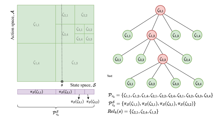
Figure 1: Adaptive discretization at episode $k$. Active cells are shown in green, and deactivated cells are shown in red. See that $\mathcal{P}_{\tau_{k}}$ partitions $\mathcal{S}\times\mathcal{A}$ and $\mathcal{P}_{\tau_{k}}^{\mathcal{S}}$ partitions $\mathcal{S}$. $\zeta_{0,1}$ is split into its child cells, $\zeta_{1,1},\zeta_{1,2}$, $\zeta_{1,3}$ and $\zeta_{1,4}$. This implies that there are enough samples to construct the estimate of the transition kernel from each of the child cells of $\zeta_{0,1}$ with confidence radii of the order of the diameter of these child cells. Similarly, there are enough samples to construct estimates of the transition kernel from the child cells of $\zeta_{1,2}$ with an acceptable confidence radius. The set of relevant cells of state $s$ in episode $k$, $\textit{Rel}_{k}{\left(s\right)}$ contains those active cells that contain $s$ in their $\mathcal{S}$-projection.

After having adaptively discretized the state-action space as discussed above, ZoRL-$\epsilon$ uses an EVI-based algorithm in order to generate a policy that has the highest UCB index. This is discussed next.

Extended Value Iteration with Bias (EVI-B): For each $s\in\mathcal{S}$, define the set of relevant cells at episode $k$ as $\textit{Rel}_{k}{\left(s\right)}:=\left\{\zeta\in\mathcal{P}_{\tau_{k}}:\exists a\in\mathcal{A}\mbox{ such that }(s,a)\in\zeta\right\}$ (See Figure 1). The EVI-B iterations are as follows,

$$\mkern 1.5mu\overline{\mkern-1.5muQ\mkern-1.5mu}\mkern 1.5mu_{0}(\zeta) =0,\quad\mkern 1.5mu\overline{\mkern-1.5muV\mkern-1.5mu}\mkern 1.5mu_{0}(s)=0$$

$$\mkern 1.5mu\overline{\mkern-1.5muQ\mkern-1.5mu}\mkern 1.5mu_{i+1}(\zeta) =r(q(\zeta))+\max_{\theta\in\bar{\mathcal{C}}_{\tau_{k}}}{\sum_{s\in S_{\tau_{k}}}{\theta(q(\zeta),s)\mkern 1.5mu\overline{\mkern-1.5muV\mkern-1.5mu}\mkern 1.5mu_{i}(s^{\prime})}}+L_{r}~{}\mbox{diam}\left(\zeta\right),~{}i\in\mathbb{Z}_{+},$$ (16)

$$\mbox{ where, }\mkern 1.5mu\overline{\mkern-1.5muV\mkern-1.5mu}\mkern 1.5mu_{i}(s): =\max_{\zeta\in\textit{Rel}_{k}{\left(s\right)}}{\mkern 1.5mu\overline{\mkern-1.5muQ\mkern-1.5mu}\mkern 1.5mu_{i}(\zeta)},\mbox{ for every }s\in\mathcal{S},i\in\mathbb{Z}_{+}.$$ (17)

Proposition C.1 in Appendix D proves that the optimal decisions generated by these iterations converge. During the $k$-th episode, ZoRL-$\epsilon$ plays the policy $\phi_{k}\in\Phi_{SD}$ such that $(s,\phi_{k}(s))\in\arg\max_{\zeta\in\textit{Rel}_{k}{\left(s\right)}}{\mkern 1.5mu\overline{\mkern-1.5muQ\mkern-1.5mu}\mkern 1.5mu_{i}(\zeta)}$ whenever $s\in\xi$ for all $\xi\in\mathcal{P}_{\tau_{k}}^{\mathcal{S}}$, for all large enough $i\in\mathbb{N}$.

Algorithm 1 Zooming algorithm for Reinforcement Learning with $\epsilon$-sub-optimal reference (ZoRL-$\epsilon$)

  Input Horizon, $T$, Lipschitz constants, $L_{r},L_{p}$, ergodicity coefficient, $\alpha$, error tolerance, $\epsilon$, lower bound constant of stationary measures, $\varrho$, confidence parameter $\delta$.

  $h=0$, $k=0$, $\mathcal{P}_{0}=\mathcal{S}\times\mathcal{A}$.

  $\tilde{\epsilon}=\epsilon/c_{s}$, $t^{\star}(\tilde{\epsilon})=\left\lceil\log{\left(\frac{2}{\varrho\tilde{\epsilon}^{d_{\mathcal{S}}}}\right)}/\log{\left(\frac{1}{\alpha}\right)}\right\rceil$.

  for $t=0$ to $T-1$ do

     if $(h\geq T/\log{\left(T\right)}$ or $N_{t}(\zeta)=N_{\max}(\zeta)$ for any $\zeta\in\mathcal{P}_{\tau_{k}}$ with $\mbox{diam}\left(\zeta\right)\geq 2\epsilon)$ $h\geq\frac{24c_{2}t^{\star}(\tilde{\epsilon})}{\tilde{\epsilon}^{2d_{\mathcal{S}}}\rho^{2}}\log{\left(\frac{T}{\delta\tilde{\epsilon}}\right)}$ then

        $k\leftarrow k+1$, $h\leftarrow 0$, $\tau_{k}=t$

        $\mathcal{P}_{\tau_{k}}=\mbox{Refine discretization}\left(\mathcal{P}_{\tau_{k-1}},\left\{\eta_{\tau_{k}}(\zeta)\mid\zeta\in\cup_{\ell}{\mathcal{P}^{(\ell)}}\right\},\epsilon\right)$  (4).

        Compute empirical estimate of discretized transition probability, $\hat{p}_{\tau_{k}}$ as in (12).

        Solve EVI-B (16) and get the policy $\phi_{k}$.

     end if

     $h\leftarrow h+1$

     Play $a_{t}=\phi_{k}(s_{t})$ and receive new state $s_{t+1}$ and reward $r(s_{t},a_{t})$.

  end for

4 Regret Analysis

We now present our main result, a regret upper bound of ZoRL-$\epsilon$. This is followed by the regret bound of the fixed discretization algorithm UCRL-C. Detailed proofs are delegated to the appendix.

Theorem 4.1.

With a probability at least $1-\delta$, the $\epsilon$-regret of ZoRL-$\epsilon$ (1) is upper-bounded as $\mathcal{O}\left(\epsilon^{-(2d_{\mathcal{S}}+d_{z}^{\epsilon}+1)}\log{\left(T\right)}\right)$.

Proof sketch:
Regret decomposition: We decompose the regret (3) in the following manner. Let $H_{k}:=\tau_{k+1}-\tau_{k}$. Then, for any learning algorithm $\psi$,

$$\mathcal{R}_{\epsilon}(T;\psi) =\sum_{k=1}^{K(T)}{\mathbbm{1}_{\left\{\Delta(\phi_{k})>\epsilon\right\}}\left(\sum_{t=\tau_{k}}^{\tau_{k+1}-1}{J^{\star}(p)-r(s_{t},a_{t})}\right)}$$

$$= \underbrace{\sum_{k=1}^{K(T)}{H_{k}\Delta(\phi_{k})\mathbbm{1}_{\left\{\Delta(\phi_{k})>\epsilon\right\}}}}_{(a)}+\underbrace{\sum_{k=1}^{K(T)}{\mathbbm{1}_{\left\{\Delta(\phi_{k})>\epsilon\right\}}\left(H_{k}~{}J(\phi_{k},p)-\sum_{t=\tau_{k}}^{\tau_{k+1}-1}{r(s_{t},\phi_{k}(s_{t}))}\right)}}_{(b)}.$$

The term (a) captures the regret component due to the gap between the optimal average reward and the average reward of the policy $\phi_{k}$ that is played during the $k$-th episode, while (b) captures the sub-optimality arising since the distribution of the induced Markov chain does not reach the stationary distribution in finite time. (a) and (b) are bounded separately below.

Bounding (a): Step 1: Define, $\mbox{diam}_{k}\left(\phi\right):=\int_{\mathcal{S}}{\mu^{(\infty)}_{p,\phi}(s)~{}\mbox{diam}\left(q_{\tau_{k}}^{-1}(s,\phi(s))\right)ds}$, where $q_{\tau_{k}}^{-1}(s,a)$ denote the active cell that contains $(s,a)$. This is the confidence radius associated with the reward estimate of $\phi$. We first show that on a high probability set, a sub-optimal policy $\phi$ will never be played from episode $k$ onwards if $\mbox{diam}_{k}\left(\phi\right)\leq\textit{const}\cdot\Delta(\phi)$, and also the maximum diameter of cells through which $\phi$ passes is at most $(1-\alpha)/3(1+L_{p})$.

Step 2: Then we show that with a high probability, if every cell in $\mathcal{Z}^{\bar{\Phi}^{\tilde{\epsilon}}}_{\gamma}$ (6) that has a diameter of $\textit{const}\cdot\gamma$ has been visited at least $\textit{const}\cdot\log{\left(T\right)}~{}\epsilon^{-d_{\mathcal{S}}}~{}\gamma^{-2}$ times until the beginning of the $k$-th episode, then no policy from $\Phi_{\gamma}$ will ever be played from episode $k$ onwards by ZoRL-$\epsilon$.

Step 3: The term (a) can be further written as the sum of the regrets arising due to playing policies from the sets $\Phi_{\gamma}$, where $\gamma$ assumes the values $2^{-i},~{}i=1,2,\ldots,\left\lceil\log{\left(\frac{1}{\epsilon}\right)}\right\rceil$. To bound the regret arising due to policies from $\Phi_{\gamma}$, we count the number of times policies from $\Phi_{\gamma}$ are played and then multiply it by $2\gamma$. We then add these regret terms from $i=1$ to $\left\lceil\log{\left(\frac{1}{\epsilon}\right)}\right\rceil$.

Bounding (b): Upper bound on the term $(b)$ relies on the geometric ergodicity property [39] of $\mathcal{M}$, that has been shown in Proposition D.4. Proposition F.4 shows that we must pay a constant penalty in regret each time we change policy, which is $\mathcal{O}(K(T))$. The rule to start a new episode of ZoRL-$\epsilon$ ensures that $K(T)$ is bounded above by $\mathcal{O}(\log{\left(T\right)})+\epsilon^{-d}$, so is the term (b).

After summing the upper bounds on (a) and (b), we obtain the desired regret bound.

Theorem 4.2.

With a probability at least $1-\delta$, the $\epsilon$-regret of UCRL-C (5) is upper bounded as $\mathcal{R}_{\epsilon}(\textit{UCRL-C};T)\leq\mathcal{O}(\epsilon^{-(2d_{\mathcal{S}}+d+1)}\log{\left(T\right)})$.

We note that due to sequential dependencies arising in MDPs, the regret analysis of UCRL-C does not follow from that of vanilla $\textit{UCRL}/\textit{UCRL-}2$ [55, 9] by adding a “discretization error term,” as is the case for Lipschitz bandits, where one can obtain regret bounds by relying upon UCB results [56]. Hence, the proof of Theorem 4.2 is quite different from that of $\textit{UCRL}/\textit{UCRL-}2$. The adaptivity gains are clearly visible upon comparing the regret expressions in Theorem 4.1 and Theorem 4.2. ZoRL-$\epsilon$  has a better $\epsilon$ dependence than UCRL-C as $d^{\epsilon}_{z}\leq d$, resulting in a tighter regret bound for benign problem instances.

5 Simulations

In this section, we compare the regret performance of ZoRL-$\epsilon$ 1 with UCRL-C 5 on two continuous MDPs with $d_{\mathcal{S}}=2$ and $d_{\mathcal{A}}=1$. Each experiment is performed for $T=10000$ and is averaged over $20$ runs. $\epsilon$ is set at $0.2$. Let us denote $s_{t,i}$ the $i$-th component of the state vector $s_{t}$. Let $\textit{Beta}(\alpha,\beta)$ denote beta distribution with parameter $\alpha$ and $\beta$.

Example I: For every $t\in\mathbb{Z}_{+}$, $s_{t+1}\sim\textit{Beta}\left(\alpha_{1},\beta_{1}\right)$, where $\alpha_{1}=\lceil 10~{}s_{t,1}(1-s_{t,2})^{2}/|a_{t}-s_{t,1}|\vee 0.1\rceil$, and $\beta_{1}=\lceil 45~{}s_{t,2}(1-s_{t,1})^{2}/|a_{t}-s_{t,2}|\vee 0.1\rceil$. The reward function is $r_{1}(s,a)=\exp{\left(-4\left\lVert s-v_{s}\right\rVert_{2}-2\left\lVert a-v_{a}\right\rVert_{2}\right)}$.

Example II: For every $t\in\mathbb{Z}_{+}$, $s_{t+1}\sim\textit{Beta}\left(\alpha_{2},\beta_{2}\right)$, where $\alpha_{1}=\lceil 100~{}s_{t,1}(1-s_{t,2})/|a_{t}-s_{t,1}|\vee 0.1\rceil$, and $\beta_{1}=\lceil 100~{}s_{t,2}(1-s_{t,1})/|a_{t}-s_{t,2}|\vee 0.1\rceil$. The reward function is unchanged.

Figure 2 shows that ZoRL-$\epsilon$  incurs comparatively better regret even for low-dimensional systems. For high dimensional systems, the improvement is expected to be much more since it is likely that $d^{\epsilon}_{z}\ll d$.

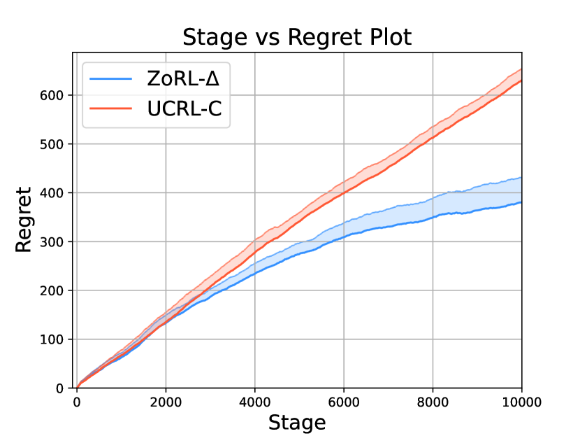
((a)) Example I

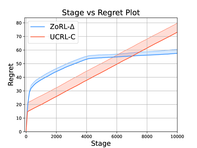
((b)) Example II

Figure 2: Cumulative Regret averaged over 20 runs.

6 Conclusion

As was seen in this work, the existing notions of zooming dimension fail to capture adaptivity gains when applied to non-episodic Lipschitz RL problems since $d_{z}\to d$ as $T\to\infty$. We have shown how to successfully employ adaptive discretization in such tasks to yield lower regrets and obtain $\mathcal{O}(\epsilon^{-(2d_{\mathcal{S}}+d_{z}^{\epsilon}+1)}\log{\left(T\right)})$ regret bound. Since the focus here was on learning algorithms with finite computation resources, we did not allow discretization beyond $\epsilon$. Future works will remove this constraint at the expense of lesser regards to computational aspects. Also, we have considered only instance-dependent regret bounds here, and the question of optimal minimax regret remains open.

Appendix A Organization of the Appendix

In Appendix B, first, the uniformly discretized MDP is introduced, followed by the continuous extension of a uniformly discretized MDP. Then, we provide the necessary algorithms for adaptive discretization. In Appendix C, we present additional definitions needed for regret analysis of ZoRL-$\epsilon$. In the next section, Appendix D, we revisit the assumption on the true MDP and deduce a few important results that we use in this work. In Appendix E, we provide the results that we have derived and are used to derive the regret upper bound of ZoRL-$\epsilon$. Next, in Appendix F, we prove the regret upper bound of ZoRL-$\epsilon$. In Appendix G, we introduce an RL algorithm, UCRL-C for Lipschitz MDPs, that is based on the upper confidence bound principle and uses the fixed discretization scheme. We also show the $\epsilon$-regret of the algorithm is bounded above as $\mathcal{O}(\epsilon^{-(2d_{\mathcal{S}}+d+1)}\log{\left(T\right)})$. In Appendix H, we have derived the regret for non-episodic RL of a straightforward extension of the algorithm proposed by [4]. Next, in Appendix I, we show some properties of EVI-B. Some useful results that we use in different places in this paper, including well-known concentration inequalities, are placed in Appendix J for reference.

Appendix B Discretization

In this section, we provide some details of the discretization procedure. The discretized MDP is created on a partition of state-action space made of “cells,” that is defined in 3.1. Let the diameter of a cell of level $\ell$ be $D~{}2^{-\ell}$. Recall $\mathcal{S}$-projection and $\mathcal{S}$-cells. The level of $\pi_{\mathcal{S}}(\zeta)$ is the same as that of $\zeta$; we denote the set of all $\mathcal{S}$-cells of level $\ell$ by $\mathcal{P}^{\mathcal{S},\ell}$.

Recall the hierarchical partitions of $\mathcal{S}\times\mathcal{A}$ from 3.2. Denote $\mathbb{C}(\zeta)$ the set of child cells of $\zeta$. It is easy to see that a parent cell is partitioned by its child cells in a partition tree.

B.1 Uniformly discretized MDP

We will now define the uniformly discretized MDP of granularity $\epsilon$, where $\epsilon\in(0,1]$. Let $\mathcal{S}^{\epsilon}:=\mathcal{S}^{\ell_{\epsilon}}$ and $\mathcal{A}^{\epsilon}:=\mathcal{A}^{\left(\ell_{\epsilon}\right)}$ where $\ell_{\epsilon}:=\left\lceil\log{\left(\frac{1}{\epsilon}\right)}\right\rceil$. Let $\mathcal{M}^{\epsilon}$ be the $\epsilon$-fine discretization of the true MDP defined as

$$\mathcal{M}^{\epsilon}:=\left(\mathcal{S}^{\epsilon},\mathcal{A}^{\epsilon},p^{\epsilon},r^{\epsilon}\right),$$ (18)

where

$$p^{\epsilon}(s,a,s^{\prime}) :=p(s,a,q^{-1}(s^{\prime})),~{}\forall s,s^{\prime}\in\mathcal{S}^{\epsilon},a\in\mathcal{A}^{\epsilon},\mbox{ and}$$ (19)

$$r^{\epsilon}(s,a) :=r(s,a),~{}\forall s\in\mathcal{S}^{\epsilon},a\in\mathcal{A}^{\epsilon}.$$ (20)

Let $\Phi^{\epsilon}_{SD}:=\left\{\phi:\mathcal{S}^{\epsilon}\to\mathcal{A}^{\epsilon}\right\}$ be the class of stationary deterministic policies for $\mathcal{M}^{\epsilon}$. Denote the optimal policy for $\mathcal{M}^{\epsilon}$ by,

$$\phi^{\star}\in\underset{\phi\in\Phi^{\epsilon}_{SD}}{\arg\max}{~{}J(\phi,p^{\epsilon})},$$ (21)

where $J(\phi,p^{\epsilon})$ is the long-term average reward of $\phi$. We define a unique extension of policy $\phi\in\Phi^{\epsilon}_{SD}$ to $\bar{\phi}\in\Phi_{SD}$ as

$$\bar{\phi}(s^{\prime})=\phi(s),~{}\forall s^{\prime}\in q^{-1}(s),s\in\mathcal{S}^{\epsilon},$$ (22)

and denote the set of all such policies by $\bar{\Phi}^{\epsilon}_{SD}$, i.e.,

$$\bar{\Phi}^{\epsilon}:=\left\{\bar{\phi}\in\Phi_{SD}:\exists\phi\in\Phi^{\epsilon}_{SD}\mbox{ s.t. }\bar{\phi}(s)=\phi(s^{\prime})~{}\forall s\in q^{-1}(s^{\prime}),s^{\prime}\in\mathcal{S}^{\epsilon}\right\}.$$ (23)

Define the continuous kernel $\bar{p}^{\epsilon}$,

$$\bar{p}^{\epsilon}(s,a,B) :=\sum_{\zeta\in\mathcal{P}^{\mathcal{S},\lceil\log{\left(\frac{1}{\epsilon}\right)}\rceil}}{p(s^{\prime},a^{\prime},\zeta)\cdot\frac{\lambda(B\cap\zeta)}{\lambda(\zeta)}},\forall B\in\mathcal{B}_{\mathcal{S}},(s,a)\in\mathcal{S}\times\mathcal{A},$$ (24)

where $\mathcal{P}^{\mathcal{S},\ell}$ deonte the set of $\mathcal{S}$-cells of level $\ell$, and the reward function $\bar{r}^{\epsilon}$,

$$\bar{r}^{\epsilon}(s,a) :=r(s^{\prime},a^{\prime}),~{}\forall(s,a)\in\mathcal{S}\times\mathcal{A},$$ (25)

where $(s^{\prime},a^{\prime})=q(\zeta)$ and $(s,a)\in\zeta\in\mathcal{P}^{\ell_{\epsilon}}$. Then the MDP $\bar{\mathcal{M}}^{\epsilon}:=(\mathcal{S},\mathcal{A},\bar{p}^{\epsilon},\bar{r}^{\epsilon})$ can be thought as a “continuous extension” of the discrete MDP $\mathcal{M}^{\epsilon}$. One can verify that $\bar{\phi}^{\star}$ is an optimal policy for $\bar{\mathcal{M}}^{\epsilon}$, where $\phi^{\star}$ is an optimal policy for $\mathcal{M}^{\epsilon}$ and $\bar{\phi}^{\star}$ is the extension of it, as in (22). In Proposition D.9, we show that $\bar{\phi}^{\star}$ is $\mathcal{O}(\epsilon)$ optimal.

B.2 Adaptive discretization

ZoRL-$\epsilon$ proceeds in episodes, i.e., it employs a policy at the beginning of every episode based on observations and plays it throughout that episode. We construct adaptively discretized MDP of the true MDP, $\mathcal{M}$, at the beginning of every episode. Recall the definition of active cells, active partition, and the activation rule 3.3. Note that the activation rule implies that when $\zeta$ ceases to be an active cell, all the child cells of $\zeta$ get activated. Since the child cells, $\mathbb{C}(\zeta)$ partitions $\zeta$, at every time the set of active cells partitions the state action space, and hence we call the set of active cells the active partition. Recall that $\mathcal{P}_{t}$ denote the active partition at time $t$, $Z_{t}=\left\{q(\zeta):\zeta\in\mathcal{P}_{t}\right\}$, and $\mathcal{P}^{\mathcal{S}}_{t}$ the least cardinality partition of $\mathcal{S}$ such that no cell in $\left\{\pi_{\mathcal{S}}(\zeta)|\zeta\in\mathcal{P}_{t}\right\}$ is a proper subset of any of the elements of $\mathcal{P}^{\mathcal{S}}_{t}$. The discrete state-space at time $t$, $S_{t}=\left\{q(\zeta):\zeta\in\mathcal{P}_{t}^{\mathcal{S}}\right\}$. The set of relevant cells of state $s$ at episode $k$,

$$\textit{Rel}_{k}{\left(s\right)}=\left\{\zeta\in\mathcal{P}_{\tau_{k}}:\exists a\in\mathcal{A}\mbox{ such that }(s,a)\in\zeta\right\},$$ (26)

where $\tau_{k}$ is the time when the $k^{\textit{th}}$ episode starts. Note that $\mathcal{P}_{\tau_{k}}^{\mathcal{S}}$ has the following property, if $s^{\prime},s^{\prime\prime}\in\zeta\in\mathcal{P}_{\tau_{k}}^{\mathcal{S}}$, then $\textit{Rel}_{k}{\left(s^{\prime}\right)}=\textit{Rel}_{k}{\left(s^{\prime\prime}\right)}$. Here we provide an algorithm, $\mathcal{S}$-partitioning (2) to find $\mathcal{P}_{\tau_{k}}^{\mathcal{S}}$ given $\mathcal{P}_{\tau_{k}}$.

Algorithm 2 $\mathcal{S}$-partitioning

  Input: A set of cells $\mathcal{P}$ that are active at time $t$

  Initilize $\mathcal{Y}=\left\{\pi_{\mathcal{S}}(\zeta):\zeta\in\mathcal{P}\right\}$

  $\ell_{\max}=\max_{\zeta\in\mathcal{P}}{\ell(\zeta)}$

  for $\ell=0$ to $\ell_{\textit{max}}-1$ do

     for $\zeta\in\mathcal{Y}$ such that $\ell(\zeta)=\ell$ do

        if $\bar{\zeta}\in\mathcal{Y}\cap\mathbb{C}(\zeta)$ then

           $\mathcal{Y}\leftarrow\mathcal{Y}\cup\mathbb{C}(\zeta)\setminus\zeta$

        end if

     end for

  end for

  Return $\mathcal{Y}$

Appendix C Algorithm

Recall that the discretized transition kernel $p_{t}$ (11) is estimated as follows,

$$\hat{p}_{t}(s,a,s^{\prime})=\frac{N_{t}\left(q^{-1}(s,a),q^{-1}(s^{\prime})\right)}{1\vee N_{t}\left(q^{-1}(s,a)\right)},~{}(s,a)\in Z_{t},s^{\prime}\in S_{t},$$ (27)

and for a cell $\zeta$, the confidence radius associated with the estimate $\hat{p}_{t}(q(\zeta),\cdot)$ is given by

$$\eta_{t}(\zeta)=3\epsilon^{-\frac{d_{\mathcal{S}}}{2}}\sqrt{\frac{c_{1}\log{\left(\frac{T}{\delta\epsilon}\right)}}{N_{t}(\zeta)}}+3L_{p}~{}\mbox{diam}\left(\zeta\right),$$ (28)

where $c_{1}$ is a constant. Note that if $\zeta\in\mathcal{P}_{t}$, then it follows from the cell activation rule 3.3 of ZoRL-$\epsilon$ that,

$$\mbox{diam}\left(\zeta\right)\geq\epsilon^{-\frac{d_{\mathcal{S}}}{2}}\sqrt{\frac{c_{1}\log{\left(\frac{T}{\delta\epsilon}\right)}}{N_{t}(\zeta)}},$$ (29)

which when combined with (28) yields,

$$\eta_{t}(\zeta)\leq 3(1+L_{p})~{}\mbox{diam}\left(\zeta\right).$$ (30)

Let us define $\Theta_{t}$, a set of discrete transition kernels, defined on all state-action pairs and with support on $S_{t}$, i.e.,

$$\Theta_{t} :=\Big{\{}\theta\mid\theta(s,a):S_{t}\to[0,1],\sum_{s^{\prime}\in S_{t}}{\theta(s,a,s^{\prime})}=1,\theta(s,a,s^{\prime})\geq 0$$

$$\qquad\mbox{ for every }(s,a)\in\mathcal{S}\times\mathcal{A}\Big{\}}.$$ (31)

Note that $p_{t}\in\Theta_{t}$. The confidence ball at time $\tau_{k}$ consists of plausible transition kernels with discretized support and is defined as follows,

$$\mathcal{C}_{t}:=\big{\{}\theta\in\Theta_{t}: \left\lVert\theta(s^{\prime},a^{\prime},\cdot)-\hat{p}_{t}(s,a,\cdot)\right\rVert_{1}\leq\eta_{t}\left(q^{-1}(s,a)\right)\mbox{ for every }(s,a)\in Z_{t},$$

$$\mbox{ for every }(s^{\prime},a^{\prime})\in q^{-1}(s,a)\big{\}},$$ (32)

where $\eta_{t}$ is as in (28). Next, we present the Extended Value Iteration with Bias (EVI-B) algorithm.

Algorithm 3 Extended Value Iteration with Bias (EVI-B)

  Input $\mathcal{P}_{\tau_{k}},\bar{\mathcal{C}}_{\tau_{k}}$, stopping criteria, $\rho$.

  Initialize $\mkern 1.5mu\overline{\mkern-1.5muQ\mkern-1.5mu}\mkern 1.5mu_{0}(\zeta)=0,~{}\mkern 1.5mu\overline{\mkern-1.5muV\mkern-1.5mu}\mkern 1.5mu_{0}(s)=0$, $i=0$.

  while True do

     $\mkern 1.5mu\overline{\mkern-1.5muQ\mkern-1.5mu}\mkern 1.5mu_{i+1}(\zeta)=r(q(\zeta))+\max_{\theta\in\bar{\mathcal{C}}_{\tau_{k}}}{\sum_{s\in S_{\tau_{k}}}{\theta(q(\zeta),s)\mkern 1.5mu\overline{\mkern-1.5muV\mkern-1.5mu}\mkern 1.5mu_{i}(s^{\prime})}}+L_{r}~{}\mbox{diam}\left(\zeta\right)$

     $\mkern 1.5mu\overline{\mkern-1.5muV\mkern-1.5mu}\mkern 1.5mu_{i}(s)=\max_{\zeta\in\textit{Rel}_{k}{\left(s\right)}}{\mkern 1.5mu\overline{\mkern-1.5muQ\mkern-1.5mu}\mkern 1.5mu_{i}(\zeta)}$, for every $s\in\mathcal{S}$

     if $\max_{s\in\mathcal{S}}{\{\mkern 1.5mu\overline{\mkern-1.5muV\mkern-1.5mu}\mkern 1.5mu_{i}(s)-\mkern 1.5mu\overline{\mkern-1.5muV\mkern-1.5mu}\mkern 1.5mu_{i}(s)\}}-\min_{s\in\mathcal{S}}{\{\mkern 1.5mu\overline{\mkern-1.5muV\mkern-1.5mu}\mkern 1.5mu_{i}(s)-\mkern 1.5mu\overline{\mkern-1.5muV\mkern-1.5mu}\mkern 1.5mu_{i}(s)\}}<\rho$ then

        Break

     end if

     $i\leftarrow i+1$

  end while

  Return $\{\arg\max_{\zeta\in\textit{Rel}_{k}{\left(s\right)}}{Q_{i}(\zeta)}\mid s\in S_{\tau_{k}}\}$

Note that we have suppressed dependence upon $k$. In case we want to depict this, then we will use $\mkern 1.5mu\overline{\mkern-1.5muV\mkern-1.5mu}\mkern 1.5mu^{(k)}_{i}(s)$, similarly for others.

Remark.

EVI-B (16) has been carefully designed so as to satisfy the following two properties: (i) the iterates $\mkern 1.5mu\overline{\mkern-1.5muQ\mkern-1.5mu}\mkern 1.5mu_{i}$ and $\mkern 1.5mu\overline{\mkern-1.5muV\mkern-1.5mu}\mkern 1.5mu_{i}$ are upper bounds on the iterates which would have been generated if one were to perform value iteration for the true MDP, and (ii) as we play a policy, its UCB bonus decreases.

The next proposition shows that the optimal decisions of EVI-B iterates converge.

Proposition C.1.

There exists $N\in\mathbb{N}$ such that for iteration steps $i>N$ a transition kernel from $\theta^{(k)}\in\bar{\mathcal{C}}_{\tau_{k}}$ and a map $\varphi^{(k)}:\mathcal{P}_{\tau_{k}}^{\mathcal{S}}\to\mathcal{P}_{\tau_{k}}$ with $\varphi^{(k)}(\xi)\in\textit{Rel}_{k}{\left(s\right)}~{}\forall s\in\xi,\xi\in\mathcal{P}_{\tau_{k}}^{\mathcal{S}}$ maximized the r.h.s. of the EVI-B (3), i.e., for every $i>N$,

$$\left(\varphi^{(k)}(\xi),\theta\right)\in\underset{\begin{subarray}{c}\zeta\in\textit{Rel}_{k}{\left(q(\xi)\right)},\\ \theta\in\bar{\mathcal{C}}_{\tau_{k}}\end{subarray}}{\arg\max}\bigg{\{} r(q(\zeta))+\max_{\theta\in\bar{\mathcal{C}}_{\tau_{k}}}{\sum_{s\in S_{\tau_{k}}}{\theta(q(\zeta),s)\mkern 1.5mu\overline{\mkern-1.5muV\mkern-1.5mu}\mkern 1.5mu_{i}(s)}}+L_{r}~{}\mbox{diam}\left(\zeta\right)\bigg{\}}.$$ (33)

Thus, for the EVI-B (3), the optimal decisions converge.

Proof.

Consider the $i$-th step of EVI-B,

$$\left(\varphi_{i}(\xi),\theta_{i}\right)\in\underset{\zeta\in\textit{Rel}_{k}{\left(q(\xi)\right)},\theta\in\bar{\mathcal{C}}_{\tau_{k}}}{\arg\max}\left\{r(q(\zeta))+\max_{\theta\in\bar{\mathcal{C}}_{\tau_{k}}}{\sum_{s\in S_{\tau_{k}}}{\theta(q(\zeta),s)\mkern 1.5mu\overline{\mkern-1.5muV\mkern-1.5mu}\mkern 1.5mu_{i}(s^{\prime})}}+L_{r}~{}\mbox{diam}\left(\zeta\right)\right\}.$$

Note that $s^{\star}:=\arg\max_{s\in S_{\tau_{k}}}{\mkern 1.5mu\overline{\mkern-1.5muV\mkern-1.5mu}\mkern 1.5mu_{i}(s)}$ is in the above set and $\theta_{i}(q(\zeta),s^{\star})\geq\min{\left\{1,\frac{1}{2}\eta_{\tau_{k}}(\zeta)\right\}}$ for all $\zeta\in\mathcal{P}_{\tau_{k}}$. Consider the stochastic matrix $\Theta$ such that $\Theta_{s,s^{\prime}}=\theta_{i}(q(\varphi_{i}(q^{-1}(s)),s^{\prime})$. It is evident that the associated Markov chain is aperiodic. The proof then follows from [7, Theorem $9.4.4$]. ∎

In episode $k$, the algorithm plays EVI-B policy $\phi_{k}\in\bar{\Phi}_{SD}^{\epsilon}$ such that $\phi_{k}(s)\in\varphi^{(k)}(\xi)$ whenever $s\in\xi$ for all $\xi\in\mathcal{P}_{\tau_{k}}^{\mathcal{S}}$, where $\varphi^{(k)}$ is as defined in (33). We say a policy $\phi\in\Phi_{SD}$ agrees with $\mathcal{P}_{\tau_{k}}$ if for each $\xi\in\mathcal{P}_{\tau_{k}}^{\mathcal{S}}$ and for all $s\in\xi$, $(s,\phi(s))\in\zeta$ for some $\zeta\in\mathcal{P}_{\tau_{k}}^{\mathcal{S}}$. We define the following iteration for $\phi\in\Phi_{SD}$ that agrees with $\mathcal{P}_{\tau_{k}}$.

$$\mkern 1.5mu\overline{\mkern-1.5muV\mkern-1.5mu}\mkern 1.5mu^{\phi}_{0}(s) =0,$$

$$\mkern 1.5mu\overline{\mkern-1.5muV\mkern-1.5mu}\mkern 1.5mu^{\phi}_{i+1}(s) =r(q(q^{-1}_{\tau_{k}}(s,\phi(s))))+\max_{\theta\in\bar{\mathcal{C}}_{\tau_{k}}}{\sum_{s^{\prime}\in S_{\tau_{k}}}{\theta(q(q^{-1}_{\tau_{k}}(s,\phi(s))),s^{\prime}){\mkern 1.5mu\overline{\mkern-1.5muV\mkern-1.5mu}\mkern 1.5mu^{\phi}_{i}(s^{\prime})}}}$$

$$\quad+L_{r}~{}\mbox{diam}\left(q^{-1}_{\tau_{k}}(s,\phi(s))\right),~{}i\in\mathbb{Z}_{+},s\in\mathcal{S}.$$ (34)

We will refer to this as index evaluation iteration, which will be useful for analyzing ZoRL-$\epsilon$. Next, we present the algorithm for updating the adaptive discretization that is used by ZoRL-$\epsilon$ 1.

Algorithm 4 Refine discretization

  Input $\mathcal{P}_{\tau_{k-1}},\left\{\eta_{\tau_{k}}(\zeta)\mid\zeta\in\cup_{\ell}{\mathcal{P}^{(\ell)}}\right\},\epsilon$.

  Initialize $\mathcal{P}_{\tau_{k}}=\mathcal{P}_{\tau_{k-1}}$, $\ell=-1$.

  while True do

     $\ell\leftarrow\ell+1$

     if $D\cdot 2^{-(\ell+1)}<\epsilon/c_{s}$ (52) then

        Break

     end if

     for $\zeta\in\left\{\zeta\mid\ell(\zeta)=\ell,\zeta\in\mathcal{P}_{\tau_{k}}\right\}$ do

        if $N_{\tau_{k}}(\zeta)\geq N_{\max}(\zeta)$ then

           $\mathcal{P}_{\tau_{k}}=\mathcal{P}_{\tau_{k}}\cup\mathbb{C}(\zeta)\setminus\{\zeta\}$

        end if

     end for

  end while

  Return $\mathcal{P}_{\tau_{k}}$

Appendix D General Results for MDPs

In this section, we revisit our assumptions on the true MDP and then provide a few important properties that the true MDP or the discretized MDPs possess under these assumptions. We use these properties while deriving the regret upper bounds.

D.1 Assumptions

Assumption D.1 (Lipschitz continuity).

1. The reward function $r$ is $L_{r}$-Lipschitz, i.e.,

   $$|r(s,a)-r(s^{\prime},a^{\prime})|\leq L_{r}\rho\left((s,a),(s^{\prime},a^{\prime})\right),$$ (35)

   $\forall s,s^{\prime}\in\mathcal{S},a,a^{\prime}\in\mathcal{A}$.

2. For a measure $\mu:\mathcal{B}_{\mathcal{S}}\mapsto\mathbb{R}$, let $\left\lVert\mu\right\rVert_{TV}$ denote its total variation norm [57], i.e.,

   $$\left\lVert\mu\right\rVert_{TV}:=\sup\left\{|\mu(B)|:B\in\mathcal{B}_{\mathcal{S}}\right\}.$$ (36)

   We assume that the transition kernel $p$ is $L_{p}$-Lipschitz, i.e.,

   $$\left\lVert p(s,a,\cdot)-p(s^{\prime},a^{\prime},\cdot)\right\rVert_{TV}\leq L_{p}\rho\left((s,a),(s^{\prime},a^{\prime})\right),$$ (37)

   $\forall s,s^{\prime}\in\mathcal{S},a,a^{\prime}\in\mathcal{A}$.

The assumption of Lipschitz MDP is one of the weakest structural assumptions on the system model. The following assumption ensures that the underlying controlled Markov process (CMP) has a “mixing” behavior. It is not restrictive since it is the weakest known sufficient condition even when the kernel $p$ is known [48] so as to ensure the existence of an optimal policy, and allows for efficient computation of optimal policy.

Assumption D.2 (Ergodicity Condition).

For each $s,s^{\prime}\in\mathcal{S}$ and $a,a^{\prime}\in\mathcal{A}$, we have

$$\left\lVert p(s,a,\cdot)-p(s^{\prime},a^{\prime},\cdot)\right\rVert_{TV}\leq 2\alpha,$$ (38)

where $\alpha\in(0,1)$.

The following recurrence condition on the underlying MDP is used to strengthen the mixing property of the MDP.

Assumption D.3.

We assume that for all policy $\phi$, the unique invariant distribution, $\mu^{(\infty)}_{\phi,p}$ is bounded away from $0$, i.e., there exists a constant $\varrho>0$ such that for every $\phi\in\Phi_{SD}$,

$$\mu^{(\infty)}_{\phi,p}(\zeta)\geq\varrho\lambda(\zeta),~{}\forall\zeta\subset\mathcal{S},$$

where $\lambda(\cdot)$ denotes the Lebesgue measure [51].

We need this assumption to ensure a sufficiently large number of visits to different parts of the state space. We note that similar or even stronger assumptions are made in the literature. For example, [53, 54] assumes that $m$ step transition kernel is bounded below by an underlying measure in order to derive concentration inequalities for ergodic Markov chains. [58] shows the consistency of the empirical risk minimization algorithm with samples generated by a uniformly ergodic Markov process and derives bounds on the rate of uniform and relative convergence. [52] considers average reward RL on continuous state space and proves that the proposed adaptive policy converges to an optimal policy. They assume that the transition kernel of the underlying MDP has a strictly positive Radon-Nikodyn derivative. Recently, [59] derived optimal sample complexity for average reward RL under the assumption that the $m$-step transition kernel is bounded below by a known measure. In another work, [41] bounds regret for average reward RL problem with linear function approximation. They assume that under every policy, the integral of cross-product of the feature vectors w.r.t. the stationary measure has all the eigenvalues bounded away from zero. This assumption ensures that upon playing any policy, the confidence ball shrinks in each direction. Similarly, our assumption ensures that the policy’s confidence diameter is reduced when played.

D.2 Implications

Consider the controlled Markov process $\{s_{t}\}$ described by the kernel $p$, which evolves under the application of a stationary policy $\phi$. The following result is an important property of controlled Markov processes that satisfy Assumption D.2 and is essentially Lemma $6.1$ of [48].

Proposition D.4.

Let $\tilde{p}:\mathcal{S}\times\mathcal{A}\times\mathcal{B}_{\mathcal{S}}\to[0,1]$ be a transition kernel that satisfies

$$\left\lVert\tilde{p}(s,a,\cdot)-\tilde{p}(s^{\prime},a^{\prime},\cdot)\right\rVert_{TV}\leq 2\alpha,$$ (39)

where $\alpha\in(0,1)$. Then, under the application of each stationary deterministic policy $\phi:\mathcal{S}\mapsto\mathcal{A}$, the controlled Markov process $\{s_{t}\}$ has a unique invariant distribution, denoted by $\mu^{(\infty)}_{\phi,\tilde{p}}$. Moreover $\{s_{t}\}$ is geometrically ergodic, i.e., for all $s\in\mathcal{S}$ the following holds,

$$\left\lVert\mu^{(t)}_{\phi,\tilde{p},s}-\mu^{(\infty)}_{\phi,\tilde{p}}\right\rVert_{TV}\leq 2\alpha^{t},~{}t\in\mathbb{N},$$ (40)

where $\mu^{(t)}_{\phi,\tilde{p},s}$ denotes the probability distribution of $s_{t}$ when $s_{0}=s$.

Proposition D.4 implies that under any $\phi\in\Phi_{SD}$, the controlled Markov process $\left\{s_{t}\right\}$ has a unique invariant distribution and is geometrically ergodic, i.e., (40) holds.

The Q-iteration for $\mathcal{M}$ [6] is defined as follows.

$$Q_{0}(s,a) =0,$$

$$Q_{i+1}(s,a) =r(s,a)+\int_{\mathcal{S}}{ds^{\prime}~{}p(s,a,s^{\prime})~{}V_{i}(s^{\prime})},~{}\forall(s,a)\in\mathcal{S}\times\mathcal{A},i\in\mathbb{Z}_{+},$$ (41)

where,

$$V_{i}(s):=\max_{a\in\mathcal{A}}{Q_{i}(s,a)},\mbox{ for every }s\in\mathcal{S},i\in\mathbb{Z}_{+}.$$ (42)

For a policy $\phi\in\Phi_{SD}$, the policy evaluation algorithm performs the following iterations,

$$V^{\phi}_{0}(s) =0,$$

$$V^{\phi}_{i+1}(s) =r(s,\phi(s))+\int_{\mathcal{S}}{ds^{\prime}~{}p(s,\phi(s),s^{\prime})~{}V^{\phi}_{i}(s^{\prime})},~{}\forall s\in\mathcal{S},i\in\mathbb{Z}_{+},$$ (43)

One can show that $\lim_{i\to\infty}{\frac{1}{i}V_{i}(s)}=J^{\star}(p)$, and $\lim_{i\to\infty}{\frac{1}{i}V^{\phi}_{i}(s)}=J(\phi,p)$ for every $s\in\mathcal{S}$ [7]. We now show another interesting property of $\mathcal{M}$ that holds under Assumption D.2.

Lemma D.5.

If the MDP $\mathcal{M}$ satisfies Assumption D.1, then for each $\phi\in\Phi_{SD}$ we have

$$~{}\textit{sp}\left(V_{i}\right)\leq\frac{1}{1-\alpha},\mbox{ and }~{}\textit{sp}\left(V^{\phi}_{i}\right)\leq\frac{1}{1-\alpha},$$ (44)

and for every $i\in\mathbb{N}$.

Proof.

We will only prove the result for $V_{i}$ since the proof of $V^{\phi}_{i}$ is similar. Consider $i\in\mathbb{Z}_{+}$. Let $\bar{s}$ be a maximizer of the function $V_{i+1}(\cdot)$, and similarly let $\underline{s}$ be a minimzer of $V_{i+1}(\cdot)$. Also, let $\bar{a}$ be an optimal action in state $\bar{s}$ that maximizes $Q_{i+1}(\bar{s},a)$, i.e.,

$$V_{i+1}(\bar{s})=r(\bar{s},\bar{a})+\int_{\mathcal{S}}{p(\bar{s},\bar{a},s^{\prime})V_{i}(s^{\prime})~{}ds^{\prime}}.$$ (45)

Similarly, let $\underline{a}$ be an action that maximizes $Q_{i+1}(\underline{s},a)$, i.e.,

$$V_{i+1}(\underline{s})=r(\underline{s},\underline{a})+\int_{\mathcal{S}}{p(\underline{s},\underline{a},s^{\prime})V_{i}(s^{\prime})~{}ds^{\prime}}.$$ (46)

$~{}\textit{sp}\left(V_{i+1}\right)$ can be upper-bounded iteratively as follows,

$$~{}\textit{sp}\left(V_{i+1}\right) =\left(r(\bar{s},\bar{a})-r(\underline{s},\underline{a})\right)+\int_{\mathcal{S}}{(p(\bar{s},\bar{a},s^{\prime})-p(\underline{s},\underline{a},s^{\prime}))V_{i}(s^{\prime})~{}ds^{\prime}}$$

$$\leq 1+\alpha~{}\textit{sp}\left(V_{i}\right),$$ (47)

where the inequality is obtained using Assumption D.2, Lemma J.6, and $\left|r(s,a)\right|\leq 1$. The claim then follows from the fact that $V_{0}=0$, and by applying (47) iteratively. ∎

The same conclusion holds for the discretized MDP that has ergodicity property with ergodicity coefficient $\alpha$.

The following lemma is essentially Corollary $3.1$ of [60].

Lemma D.6 (Mitrophanov).

Let $P_{1}$ and $P_{2}$ be transition kernels of two Markov chains on the same state space $\bar{\mathcal{S}}$. Let $\sup_{s\in\bar{\mathcal{S}}}{\left\lVert\left(P_{1}-P_{2}\right)(s)\right\rVert_{TV}}\leq\epsilon$. If $P_{1}$ is uniformly ergodic with unique invariant distribution $\mu_{1}$ such that

$$\sup_{s\in\bar{\mathcal{S}},x_{0}\in\bar{\mathcal{S}}}{\left|\mu^{(t)}_{1,x_{0}}(s)-\mu_{1}(s)\right|}\leq 2\alpha^{t},$$

for some $c\in\mathbb{R}_{+}$, for all $t\in\mathbb{Z}_{+}$, where $\mu^{(t)}_{1,x_{0}}$ denote distribution of states at time $t$ given the start state be $x_{0}$. Let the invariant distribution of $P_{2}$ exists and be denoted by $\mu_{2}$. Then,

$$\left\lVert\mu_{1}-\mu_{2}\right\rVert_{TV}\leq\left(\hat{n}+\frac{2\alpha^{\hat{n}}}{1-\alpha}\right)\epsilon,$$

where, $\hat{n}=\left\lceil\log_{\alpha}{\left(\frac{1}{2}\right)}\right\rceil$.

Corollary D.7.

Let $\phi_{1}$ and $\phi_{2}$ are two policies for $\mathcal{M}$ as defined in (18). Then

$$\left|J(\phi_{1},p)-J(\phi_{2},p)\right|\leq\frac{L_{p}}{2}\left(\hat{n}+\frac{2\alpha^{\hat{n}}}{1-\alpha}\right)\rho_{\phi}\left(\phi_{1},\phi_{2}\right),$$

where $\rho_{\phi}$ is as defined as

$$\rho_{\phi}(\phi_{1},\phi_{2}):=\sup_{s\in\mathcal{S}}{\rho_{\mathcal{A}}(\phi_{1}(s),\phi_{2}(s))}.$$ (48)

Proof.

By Assumption (ii), $\left\lVert p(s,\phi_{1}(s))-p(s,\phi_{2}(s))\right\rVert_{TV}\leq L_{p}\rho_{\phi}(\phi_{1},\phi_{2})$. Now, by D.6, we have the bound on total variation distance between the stationary distributions of the Markov chains induced by policies, $\phi_{1}$ and $\phi_{2}$.

$$\left\lVert\mu^{(\infty)}_{\phi_{1},p}-\mu^{(\infty)}_{\phi_{2},p}\right\rVert_{TV} \leq L_{p}\left(\hat{n}+\frac{2\alpha^{\hat{n}}}{1-\alpha}\right)\rho_{\phi}\left(\phi_{1},\phi_{2}\right).$$

Using this, we get the lemma.

$$\left|J(\phi_{1},p)-J(\phi_{2},p)\right| \leq\left|\int_{\mathcal{S}}{\left(\mu^{(\infty)}_{\phi_{1},p}(s)-\mu^{(\infty)}_{\phi_{2},p}(s)\right)r(s,\phi(s))ds}\right|$$

$$\leq\frac{1}{2}\left\lVert\mu^{(\infty)}_{\phi_{1},p}-\mu^{(\infty)}_{\phi_{2},p}\right\rVert_{TV}$$

$$\leq\frac{L_{p}}{2}\left(\hat{n}+\frac{2\alpha^{\hat{n}}}{1-\alpha}\right)\rho_{\phi}\left(\phi_{1},\phi_{2}\right).$$ (49)

∎

The following result shows that under Assumption D.2, any discrete MDP obtained from $\mathcal{M}$ is unichain and geometrically ergodic.

Proposition D.8.

Under Assumption D.2, $\mathcal{M}^{\epsilon}$ (18) is unichain. Moreover, for any stationary policy $\phi$,

$$\left\lVert\mu^{(t)}_{\phi,p^{\epsilon},s}-\mu^{(\infty)}_{\phi,p^{\epsilon}}\right\rVert_{TV}\leq 2\alpha^{t},~{}t=1,2,\ldots.$$ (50)

Proof.

We begin by showing the following: consider two discretized state-action pairs $(s,a)$ and $(s^{\prime},a^{\prime})$ belonging to $\mathcal{S}^{\epsilon}\times\mathcal{A}^{\epsilon}$. Then, there exists a cell $\zeta\in\mathcal{P}^{\epsilon}$ such that we have

$$p(s,a,\zeta)>0,\mbox{ and }p(s^{\prime},a^{\prime},\zeta)>0.$$

On the contrary, let’s assume that for each interval $\tilde{\zeta}\in\mathcal{P}^{\epsilon}$, either $p(s,a,\tilde{\zeta})>0,p(s^{\prime},a^{\prime},\tilde{\zeta})=0$ (cells of type $1$), or $p(s,a,\tilde{\zeta})=0,p(s^{\prime},a^{\prime},\tilde{\zeta})>0$ (type $2$). This would mean that the measure $p(s,a,\tilde{\zeta})$ assigns a mass of $1$ to the union of type $1$ cells, while $p(s^{\prime},a^{\prime},\cdot)$ assigns a mass of $1$ to the union of type $2$ cells, where the intersection of type 1 cells with type $2$ cells is empty. This would mean that $\left\lVert p(s,a,\cdot)-p(s^{\prime},a^{\prime},\cdot)\right\rVert_{TV}=2$, which contradicts Assumption D.2. Consequently, we have shown the following property: for each $(s,a),(s^{\prime},a^{\prime})$, there exists a $\tilde{s}\in\mathcal{S}^{\epsilon}$ such that $p^{\epsilon}(s,a,\tilde{s}),p^{\epsilon}(s^{\prime},a^{\prime},\tilde{s})>0$.

Now, if $\mathcal{M}^{\epsilon}$ were not unichain, there would be a stationary policy $\phi\in\Phi^{\epsilon}_{SD}$ under which there would be two separate recurrent classes. Let $s_{1},s_{2}$ belong to these two recurrent classes. Now consider the state-action pairs $(s_{1},\phi(s_{1}))$ and $(s_{2},\phi(s_{2}))$. Since $s_{1},s_{2}$ belong to separate classes under $\phi$, we have that $p^{\epsilon}(s_{1},\phi(s_{1}),\cdot)$ and $p^{\epsilon}(s_{2},\phi(s_{2}),\cdot)$ live on mutually orthogonal sets. This, however, contradicts the property which was shown in the previous paragraph. Hence, we conclude that $\mathcal{M}^{\epsilon}$ is unichain.

To show (50) we will show that $p^{\epsilon}$ satisfies (38). The claim would then follow from Proposition D.4. We have

$$\|p^{\epsilon}(s,a,\cdot)-p^{\epsilon}(s^{\prime},a^{\prime},\cdot)\|_{TV} =2\sup_{\tilde{s}\in\mathcal{S}^{\epsilon}}|p^{\epsilon}(s,a,\zeta^{\epsilon}_{y})-p(s^{\prime},a^{\prime},\zeta^{\epsilon}_{y})|$$

$$\leq 2\sup_{B\in\mathcal{B}_{X}}|p(s,a,B)-p(s^{\prime},a^{\prime},B)|$$

$$\leq 2\alpha,$$ (51)

where the last inequality follows from Assumption D.2. ∎

Remark.

The results in the last proposition hold true for any discretized MDP created out of $\mathcal{M}$.

Proposition D.9.

Let $\mathcal{M}$ satisfy Assumptions D.1 and D.2. We then have that,

$$J^{\star}(p)-J(\bar{\phi}^{\star},p)\leq c_{s}\cdot\epsilon,$$

where,

$$c_{s}:=2\left(L_{r}+L_{p}\left(\hat{n}+\frac{2\alpha^{\hat{n}}}{1-\alpha}\right)\right),$$ (52)

and

$$\hat{n}:=\Big{\lceil}\log_{\alpha}{\left(1/2\right)}\Big{\rceil},$$ (53)

$L_{r},L_{p}$ are as in Assumption D.1, $\alpha$ is as in Assumption D.2. Hence, the best policy for $\bar{\mathcal{M}}^{\epsilon}$ is at most $c_{s}\cdot\epsilon$-sub-optimal for the true MDP $\mathcal{M}$.

Proof.

We begin by decomposing the term that we need to bound.

$$J^{\star}(p)-J(\bar{\phi}^{\star},p) =J^{\star}(p)-J(\bar{\phi}^{\star},\bar{p}^{\epsilon})+J(\bar{\phi}^{\star},\bar{p}^{\epsilon})-J(\bar{\phi}^{\star},p)$$

$$\leq J(\tilde{\phi}^{\star},p)-J(\tilde{\phi}^{\star},\bar{p}^{\epsilon})+J(\bar{\phi}^{\star},\bar{p}^{\epsilon})-J(\bar{\phi}^{\star},p),$$ (54)

where $\tilde{\phi}^{\star}:\mathcal{S}\to\mathcal{A}$ be an optimal policy for the original MDP $\mathcal{M}$. The last inequality above uses the fact $J(\tilde{\phi}^{\star},\bar{p}^{\epsilon})\leq J(\bar{\phi}^{\star},\bar{p}^{\epsilon})$. It follows from Proposition D.4 that since $p$ and $\bar{p}^{\epsilon}$ satisfy Assumption D.2, when any policy $\phi$ is applied to the kernel $p$ or $\bar{p}^{\epsilon}$, the resulting process is geometrically ergodic and it has a unique invariant probability measure. Also, note that it follows from Assumption D.1-(ii) that for any policy $\phi$, $\left\lVert p(s,\phi(s),\cdot)-\bar{p}^{\epsilon}(s,\phi(s),\cdot)\right\rVert_{TV}\leq\epsilon L_{p}$. Hence, it follows from Corollary 3.1 of [60] that,

$$\|\mu^{(\infty)}_{\tilde{\phi}^{\star},p}-\mu^{(\infty)}_{\tilde{\phi}^{\star},\bar{p}^{\epsilon}}\|_{TV} \leq\epsilon L_{p}\left(\hat{n}+\frac{2\alpha^{\hat{n}}}{1-\alpha}\right),\mbox{ and}$$ (55)

$$\|\mu^{(\infty)}_{\bar{\phi}^{\star},p}-\mu^{(\infty)}_{\bar{\phi}^{\star},\bar{p}^{\epsilon}}\|_{TV} \leq\epsilon L_{p}\left(\hat{n}+\frac{2\alpha^{\hat{n}}}{1-\alpha}\right),$$ (56)

where $\hat{n}$ is as in (53). Now,

$$\left|J(\tilde{\phi}^{\star},p)-J(\tilde{\phi}^{\star},\bar{p}^{\epsilon})\right| =\left|\int{r(s,\tilde{\phi}^{\star}(s))d\mu^{(\infty)}_{\tilde{\phi}^{\star},p}(s)}-\int{\bar{r}^{\epsilon}(s,\tilde{\phi}^{\star}(s))d\mu^{(\infty)}_{\tilde{\phi}^{\star},\bar{p}^{\epsilon}}(s)}\right|$$

$$\leq\left|\int{r(s,\tilde{\phi}^{\star}(s))d\mu^{(\infty)}_{\tilde{\phi}^{\star},p}(s)}-\int{\bar{r}^{\epsilon}(s,\tilde{\phi}^{\star}(s))d\mu^{(\infty)}_{\tilde{\phi}^{\star},p}(s)}\right|$$

$$+\left|\int{\bar{r}^{\epsilon}(s,\tilde{\phi}^{\star}(s))d\mu^{(\infty)}_{\tilde{\phi}^{\star},p}(s)}-\int{\bar{r}^{\epsilon}(s,\tilde{\phi}^{\star}(s))d\mu^{(\infty)}_{\tilde{\phi}^{\star},\bar{p}^{\epsilon}}(s)}\right|$$

$$\leq\epsilon L_{r}+\epsilon L_{p}\left(\hat{n}+\frac{2\alpha^{\hat{n}}}{1-\alpha}\right),$$ (57)

where the last inequality follows from (55) and from Assumption D.1-(i). Using a similar argument, one can show from (56) that

$$\left|J(\bar{\phi}^{\star},\bar{p}^{\epsilon})-J(\bar{\phi}^{\star},p)\right|\leq\epsilon L_{r}+\epsilon L_{p}\left(\hat{n}+\frac{2\alpha^{\hat{n}}}{1-\alpha}\right)$$ (58)

The proof then follows by combining (54), (57) and (58). ∎

Appendix E Auxiliary Results

Lemma E.1.

For all $t\in[T-1]$ and $\zeta\in\mathcal{P}_{t}$, let $t_{i}$ denote the time instance when $\zeta$ or any of its ancestor was visited by the algorithm for the $i$-th time. Then

$$\frac{1}{N_{t}(\zeta)}\sum_{i=1}^{N_{t}(\zeta)}{\mbox{diam}\left(\zeta_{t_{i}}\right)}\leq 3~{}\mbox{diam}\left(\zeta\right).$$

Proof.

By the activation rule (3.3), any cell, $\zeta^{\prime}$ is played at most $N_{\max}(\zeta^{\prime})-N_{\min}(\zeta^{\prime})=\tilde{c}_{1}2^{2\ell(\zeta^{\prime})}+\frac{\tilde{c}_{1}}{3}\mathbbm{1}_{\left\{\zeta^{\prime}=\mathcal{S}\times\mathcal{A}\right\}}$ times while being active, where $\tilde{c}_{1}=3c_{1}D^{-2}\log{\left(\frac{T}{\epsilon\delta}\right)}~{}\epsilon^{-d_{\mathcal{S}}}$. We can write,

$$\frac{1}{N_{t}(\zeta)}\sum_{i=1}^{N_{t}(\zeta)}{\mbox{diam}\left(\zeta_{t_{i}}\right)} =\frac{1}{N_{t}(\zeta)}\sum_{i=1}^{N_{\min}(\zeta)}{\mbox{diam}\left(\zeta_{t_{i}}\right)}+\frac{1}{N_{t}(\zeta)}\sum_{i=N_{\min}(\zeta)+1}^{N_{t}(\zeta)}{\mbox{diam}\left(\zeta_{t_{i}}\right)}$$

$$=\frac{\tilde{c}_{1}D}{3N_{t}(\zeta)}+\frac{\tilde{c}_{1}D}{N_{t}(\zeta)}\sum_{\ell=0}^{\ell(\zeta)-1}{2^{\ell}}+\frac{N_{t}(\zeta)-N_{\min}(\zeta)-1}{N_{t}(\zeta)}\mbox{diam}\left(\zeta\right)$$

$$<\frac{\tilde{c}_{1}D}{N_{t}(\zeta)}2^{\ell(\zeta)}+\frac{N_{t}(\zeta)-N_{\min}(\zeta)-1}{N_{t}(\zeta)}\mbox{diam}\left(\zeta\right)$$

$$=\frac{3N_{\min}(\zeta)}{N_{t}(\zeta)}\mbox{diam}\left(\zeta\right)+\frac{N_{t}(\zeta)-N_{\min}(\zeta)-1}{N_{t}(\zeta)}\mbox{diam}\left(\zeta\right)$$

$$=\frac{(N_{t}(\zeta)+2N_{\min}(\zeta)-1)~{}\mbox{diam}\left(\zeta\right)}{N_{t}(\zeta)}$$

$$\leq 3~{}\mbox{diam}\left(\zeta\right),$$

where the last step is due to the fact that $N_{\min}(\zeta)\leq N_{t}(\zeta)$. ∎

E.1 Concentration Inequality

Recall confidence ball, $\mathcal{C}_{t}$ from (C). Consider the following event,

$$\mathcal{G}_{1}:=\cap_{t=0}^{T-1}{\left\{p_{t}\in\mathcal{C}_{t}\right\}},$$ (59)

on which the true MDP belongs to the confidence balls at each time $t$. We will establish certain properties of ZoRL-$\epsilon$ on $\mathcal{G}_{1}$. Note that $\cap_{k}{\left\{p_{\tau_{k}}\in\mathcal{C}_{\tau_{k}}\right\}}\subset\mathcal{G}_{1}$ and $\cap_{k}{\left\{\bar{p}_{\tau_{k}}\in\bar{\mathcal{C}}_{\tau_{k}}\right\}}\subset\mathcal{G}_{1}$. We show that $\mathcal{G}_{1}$ holds with a high probability.

Lemma E.2.

$\mathbb{P}(\mathcal{G}_{1})\geq 1-\frac{\delta}{2}$, where $\mathcal{G}_{1}$ is as in (59).

Proof.

Fix $t$, and consider a point $z\in Z_{t}$. Within this proof, we denote $q^{-1}_{t}(z)$ by $\zeta$. Let $\zeta$ be a cell of level $\ell$ and note that $\zeta$ is an active cell at time $t$. Let $z^{\prime}$ be an arbitrary point in $\zeta$. We want to get a high probability bound on $\left\lVert\hat{p}_{t}(z,\cdot)-p_{t}(z^{\prime},\cdot)\right\rVert_{1}$. Note that both $\hat{p}_{t}(z,\cdot)$ and $p_{t}(z^{\prime},\cdot)$ has support $\mathcal{S}_{t}$ and $\left|\mathcal{S}_{t}\right|\leq\tilde{\epsilon}^{-d_{\mathcal{S}}}$.

We have,

$$\left\lVert\hat{p}_{t}(z,\cdot)-p_{t}(z^{\prime},\cdot)\right\rVert_{1}=2\max_{A\in\mathcal{S}_{t}}{\sum_{\tilde{s}\in A}{\hat{p}_{t}(z,\tilde{s})-p_{t}(z^{\prime},\tilde{s})}}.$$

Let $\mathcal{S}^{+}_{t}$ denote the collection of points of $\mathcal{S}_{t}$ such that for any $\tilde{s}\in\mathcal{S}^{+}_{t}$, we have $\hat{p}_{t}(z,\tilde{s})-p_{t}(z^{\prime},\tilde{s})>0$. Note that if $A\subset\mathcal{S}^{+}_{t}$, then $\mathcal{S}_{t}\setminus A\not\subset\mathcal{S}^{+}_{t}$. Hence the number of subsets of $\mathcal{S}^{+}_{t}$ is at most $2^{|\mathcal{S}_{t}|-1}$. Also, we have the following.

$$\mathbb{P}\left(\left\lVert\hat{p}_{t}(z,\cdot)-p_{t}(z^{\prime},\cdot)\right\rVert_{1}\geq\iota\right) =\mathbb{P}\left(\max_{\tilde{\xi}\subset\mathcal{S}^{+}_{t}}{\sum_{\tilde{s}\in\tilde{\xi}}{\hat{p}_{t}(z,\tilde{s})-p_{t}(z^{\prime},\tilde{s})}}\geq\frac{\iota}{2}\right)$$

$$=\mathbb{P}\left(\cup_{\tilde{\xi}\subset\mathcal{S}^{+}_{t}}{\left\{\sum_{\tilde{s}\in\tilde{\xi}}{\hat{p}_{t}(z,\tilde{s})-p_{t}(z^{\prime},\tilde{s})\geq\frac{\iota}{2}}\right\}}\right).$$ (60)

If $\mathbb{P}\left(\sum_{\tilde{s}\in\tilde{\xi}}{\hat{p}_{t}(z,\tilde{s})-p_{t}(z^{\prime},\tilde{s})\geq\frac{\iota}{2}}\right)\leq b_{\iota},~{}\forall\tilde{\xi}\subset\mathcal{S}^{+}_{t}$, then by an application of union bound we obtain that the following must hold,

$$\mathbb{P}\left(\left\lVert\hat{p}_{t}(z,\cdot)-p_{t}(z^{\prime},\cdot)\right\rVert_{1}\geq\iota\right)\leq 2^{|\mathcal{S}_{t}|-1}b_{\iota}.$$ (61)

Consider a fixed $\xi\subset\mathcal{S}$. Define the following random processes,

$$v_{i}(z) :=\mathbbm{1}_{\left\{(s_{i},a_{i})\in\zeta_{i}\right\}},$$ (62)

$$v_{i}(z,\xi) :=\mathbbm{1}_{\left\{(s_{i},a_{i},s_{i+1})\in\zeta_{i}\times\xi\right\}},$$ (63)

$$w_{i}(z,\xi) :=v_{i}(z,\xi)-p(s_{i},a_{i},\xi)v_{i}(z),$$ (64)

where $i\in\left[T-1\right]$. Let $\tilde{\xi}\subset\mathcal{S}^{+}_{t}$ and $\xi=\cup_{\tilde{s}\in\tilde{\xi}}{q^{-1}(\tilde{s})}$. Then we have,

$$\sum_{\tilde{s}\in\tilde{\xi}}{\hat{p}_{t}(z,\tilde{s})-p_{t}(z^{\prime},\tilde{s})} =\frac{N_{t}\left(\zeta,\xi\right)}{N_{t}\left(\zeta\right)}-p(z^{\prime},\xi)$$

$$=\frac{N_{t}\left(\zeta,\xi\right)-p(z^{\prime},\xi)N_{t}\left(\zeta\right)}{N_{t}\left(\zeta\right)}$$

$$\leq\frac{1}{N_{t}\left(\zeta\right)}\left(\sum_{i=0}^{t-1}{w_{i}(z,\xi)}\right)+\frac{L_{p}}{2N_{t}\left(\zeta\right)}\sum_{i=0}^{N_{t}(\zeta)}{\mbox{diam}\left(\zeta_{t_{i}}\right)}$$

$$\leq\frac{1}{N_{t}\left(\zeta\right)}\left(\sum_{i=0}^{t-1}{w_{i}(z,\xi)}\right)+1.5L_{p}~{}\mbox{diam}\left(\zeta\right),$$ (65)

where the last step follows from Lemma E.1. Note that $\left\{w_{i}(z,\zeta)\right\}_{i\in[T-1]}$ is martingale difference sequence w.r.t. $\left\{\mathcal{F}_{i}\right\}_{i\in[T-1]}$. Moreover, $\left|w_{i}(z,\zeta)\right|\leq 1$. Hence from Theorem J.1 we have,

$$\mathbb{P}\left(\left\{\frac{\sum_{i=0}^{t-1}{w_{i}(s,a,\xi)}}{N_{t}\left(\zeta\right)}\geq\sqrt{\frac{2}{N_{t}(\zeta)}\log{\left(\frac{1}{\delta}\right)}}\right\}\right)\leq\frac{\delta}{2},$$

which when combined with (65) yields,

$$\mathbb{P}\left(\hat{p}_{t}(z,\bar{\xi})-p_{t}(z^{\prime},\bar{\xi})\geq\sqrt{\frac{2}{N_{t}(\zeta)}\log{\left(\frac{2T\mathcal{N}_{1}}{\delta}\right)}}+1.5L_{p}~{}\mbox{diam}\left(\zeta\right)\right)\leq\frac{\delta}{2T\mathcal{N}_{1}},$$

where $\mathcal{N}_{1}=2\left(\frac{c_{s}D}{\epsilon}\right)^{d}$ is the number of cells the algorithm can activate under all sample paths. Upon using (61) in the above, we obtain,

$$\mathbb{P}\left(\left\lVert\hat{p}_{t}(z,\cdot)-p_{t}(z^{\prime},\cdot)\right\rVert_{1}\geq\sqrt{\frac{8\left|S_{t}\right|}{N_{t}(\zeta)}\log{\left(\frac{2T\mathcal{N}_{1}}{\delta}\right)}}+3L_{p}~{}\mbox{diam}\left(\zeta\right)\right)\leq\frac{\delta}{2T\mathcal{N}_{1}}.$$

Replacing $\left|\mathcal{S}_{t}\right|$ by its upper bound $\tilde{\epsilon}^{-d_{\mathcal{S}}}$, we have,

$$\mathbb{P}\left(\left\lVert\hat{p}_{t}(z,\cdot)-p_{t}(z^{\prime},\cdot)\right\rVert_{1}\geq 3~{}\tilde{\epsilon}^{-\frac{d_{\mathcal{S}}}{2}}\sqrt{\frac{\log{\left(\frac{2T\mathcal{N}_{1}}{\delta}\right)}}{N_{t}(\zeta)}}+3L_{p}~{}\mbox{diam}\left(\zeta\right)\right)\leq\frac{\delta}{2T\mathcal{N}_{1}}.$$ (66)

Upon taking union bound over all cells that could be activated in all sample paths combined and all possible values of $t$, the above inequality yields that with a probability at least $1-\frac{\delta}{2}$, the following holds,

$$\left\lVert\hat{p}_{t}(z,\cdot)-p_{t}(z^{\prime},\cdot)\right\rVert_{1} \leq 3~{}\epsilon^{-\frac{d_{\mathcal{S}}}{2}}\sqrt{\frac{c_{1}\log{\left(\frac{T}{\epsilon\delta}\right)}}{N_{t}(\zeta)}}+3L_{p}~{}\mbox{diam}\left(\zeta\right),$$ (67)

for every $z\in Z_{t}$, $t\in[T-1]$, where $c_{1}$ be a constant such that $c_{s}^{d_{\mathcal{S}}/2}\log{\left(\frac{2T\mathcal{N}_{1}}{\delta}\right)}=c_{1}\log{\left(\frac{T}{\epsilon\delta}\right)}$. ∎

E.2 Properties of the Extended Value Iterates

We will now show that the EVI-B iterates (3) [9, 38] are optimistic estimates of the true Q-function on the set $\mathcal{G}_{1}$, i.e. $\mkern 1.5mu\overline{\mkern-1.5muQ\mkern-1.5mu}\mkern 1.5mu_{i}(\zeta)\geq Q_{i}(s,a),\zeta\in\mathcal{P}_{\tau_{k}},(s,a)\in\zeta,i\in\mathbb{N}$.

Lemma E.3 (Optimism).

Consider the EVI-B (3). On the set $\mathcal{G}_{1}$, we have, for all $i\in\mathbb{N}$

$$\mkern 1.5mu\overline{\mkern-1.5muQ\mkern-1.5mu}\mkern 1.5mu_{i}(\zeta) \geq Q_{i}(z),~{}\forall\zeta\in\mathcal{P}_{\tau_{k}},z\in\zeta,$$ (68)

$$\mkern 1.5mu\overline{\mkern-1.5muV\mkern-1.5mu}\mkern 1.5mu_{i}(s) \geq V_{i}(s),~{}\forall s\in\mathcal{S}.$$ (69)

where $Q_{i}$ and $V_{i}$ are as defined in (41) and (42) respectively.

Proof.

We prove this using induction. The base cases (for $i=0$) hold trivially. Next, assume that the following hold for all $j\in[i]$, where $i\in\mathbb{N}$,

$$\mkern 1.5mu\overline{\mkern-1.5muQ\mkern-1.5mu}\mkern 1.5mu_{j}(\zeta) \geq Q_{j}(z),~{}\forall\zeta\in\mathcal{P}_{\tau_{k}},z\in\zeta,$$ (70)

$$\mkern 1.5mu\overline{\mkern-1.5muV\mkern-1.5mu}\mkern 1.5mu_{j}(s) \geq V_{j}(s),~{}\forall s\in\mathcal{S}.$$ (71)

Consider a cell $\zeta\in\mathcal{P}_{\tau_{k}}$, and a $z\in\zeta$. Then,

$$\mkern 1.5mu\overline{\mkern-1.5muQ\mkern-1.5mu}\mkern 1.5mu_{i+1}(\zeta) =r(q(\zeta))+\max_{\theta\in\bar{\mathcal{C}}_{\tau_{k}}}{\sum_{s^{\prime}\in\mathcal{S}_{\tau_{k}}}{\theta(q(\zeta),s^{\prime})\mkern 1.5mu\overline{\mkern-1.5muV\mkern-1.5mu}\mkern 1.5mu_{i}(s^{\prime})}}+L_{r}\mbox{diam}\left(\zeta\right)$$

$$\geq r(z)+\sum_{s^{\prime}\in\mathcal{S}_{\tau_{k}}}{p(z,q^{-1}(s^{\prime}))\mkern 1.5mu\overline{\mkern-1.5muV\mkern-1.5mu}\mkern 1.5mu_{i}(s^{\prime})}-\left|r(z)-r(q(\zeta))\right|+L_{r}\mbox{diam}\left(\zeta\right)$$

$$\geq r(z)+\int_{\mathcal{S}}{ds^{\prime}~{}p(z,s^{\prime})V_{i}(s^{\prime})}-L_{r}\mbox{diam}\left(\zeta\right)+L_{r}\mbox{diam}\left(\zeta\right)$$

$$\geq Q_{i+1}(z),$$

where the first inequality follows from the definition of $\bar{\mathcal{C}}_{\tau_{k}}$ (C), $\mathcal{G}_{1}$ (59), the second inequality follows from (71), and the third inequality follows from Assumption (D.1). Hence, we have shown that (68) holds for step $i+1$.

We will now show that (71) holds for $i+1$. Fix $s\in\mathcal{S}$. Since we have shown above that $\mkern 1.5mu\overline{\mkern-1.5muQ\mkern-1.5mu}\mkern 1.5mu_{i+1}(\zeta)\geq Q_{i+1}(s,a)$ for all $(s,a)\in\zeta$, we have,

$$\mkern 1.5mu\overline{\mkern-1.5muV\mkern-1.5mu}\mkern 1.5mu_{i+1}(s) =\max_{\zeta\in\textit{Rel}_{k}{\left(s\right)}}{\mkern 1.5mu\overline{\mkern-1.5muQ\mkern-1.5mu}\mkern 1.5mu_{i+1}(\zeta)}$$

$$\geq\max_{a\in\mathcal{A}}{Q_{i+1}(s,a)}$$

$$\geq V_{i+1}(s).$$

This concludes the proof. ∎

Consider a policy $\phi\in\Phi_{SD}$ that agrees with the $\mathcal{P}_{\tau_{k}}$. The next result establishes a relation between iterates generated by policy evaluation (43) and the iterations (34) which generate the optimistic value of $\phi$.

Lemma E.4.

For consider an episode $k\in\mathbb{Z}_{+}$ and a policy $\phi\in\Phi_{SD}$ such that

$$\max_{s\in\mathcal{S}}{\mbox{diam}\left(q^{-1}_{\tau_{k}}(s,\phi(s))\right)}\leq\frac{1-\alpha}{3(1+L_{p})},$$ (72)

then we have, for all $i\in\mathbb{Z}_{+}$,

$$\mkern 1.5mu\overline{\mkern-1.5muV\mkern-1.5mu}\mkern 1.5mu^{\phi}_{i}(s)\leq V^{\phi}_{i}(s)+C_{1}~{}\mathbb{E}\left[\sum_{j=0}^{i-1}{\mbox{diam}\left(q_{\tau_{k}}^{-1}(s_{j},\phi(s_{j}))\right)}\middle|s_{0}=s\right],~{}\forall s\in\mathcal{S},$$ (73)

where

$$C_{1}:=3\left(L_{r}+\frac{1+L_{p}}{1-\alpha}\right),$$ (74)

and $V^{\phi}_{i},\mkern 1.5mu\overline{\mkern-1.5muV\mkern-1.5mu}\mkern 1.5mu^{\phi}_{i}$ are as in (43) and (34) respectively.

Proof.

We first show that if $\phi$ satisfies (72), then for every $i\in\mathbb{Z}_{+}$, $~{}\textit{sp}\left(\mkern 1.5mu\overline{\mkern-1.5muV\mkern-1.5mu}\mkern 1.5mu^{\phi}_{i}\right)$ is bounded by $\frac{2}{1-\alpha}+\frac{2L_{r}}{3(1+L_{p})}$. Denote $q^{-1}_{\tau_{k}}(s,\phi(s))$ by $\zeta^{\phi}_{s}$. Note that,

$$\mkern 1.5mu\overline{\mkern-1.5muV\mkern-1.5mu}\mkern 1.5mu^{\phi}_{i+1}(s) =r(q(\zeta^{\phi}_{s}))+\max_{\theta\in\bar{\mathcal{C}}_{\tau_{k}}}{\sum_{s^{\prime}\in\mathcal{S}_{\tau_{k}}}{\theta(q(\zeta^{\phi}_{s}),s^{\prime})\mkern 1.5mu\overline{\mkern-1.5muV\mkern-1.5mu}\mkern 1.5mu^{\phi}_{i}(s^{\prime})}}+L_{r}~{}\mbox{diam}\left(\zeta^{\phi}_{s}\right)$$

$$\leq r(q(\zeta^{\phi}_{s}))+\sum_{s^{\prime}\in\mathcal{S}_{\tau_{k}}}{p_{\tau_{k}}(q(\zeta^{\phi}_{s}),s^{\prime})\mkern 1.5mu\overline{\mkern-1.5muV\mkern-1.5mu}\mkern 1.5mu^{\phi}_{i}(s^{\prime})}+1.5(1+L_{p})~{}\textit{sp}\left(\mkern 1.5mu\overline{\mkern-1.5muV\mkern-1.5mu}\mkern 1.5mu^{\phi}_{i}\right)\mbox{diam}\left(\zeta^{\phi}_{s}\right)$$

$$\quad+L_{r}~{}\mbox{diam}\left(\zeta^{\phi}_{s}\right),$$

where the inequality is due to (30) and Lemma J.6. Now, since (72) holds, we take the difference of $\mkern 1.5mu\overline{\mkern-1.5muV\mkern-1.5mu}\mkern 1.5mu^{\phi}_{i+1}$ at any two points, and upon taking a maximum over all pair of points, we get

$$~{}\textit{sp}\left(\mkern 1.5mu\overline{\mkern-1.5muV\mkern-1.5mu}\mkern 1.5mu^{\phi}_{i+1}\right)\leq 1+\frac{L_{r}(1-\alpha)}{3(1+L_{p})}+\frac{1+\alpha}{2}~{}\textit{sp}\left(\mkern 1.5mu\overline{\mkern-1.5muV\mkern-1.5mu}\mkern 1.5mu^{\phi}_{i}\right).$$

A few steps of algebraic manipulation yields that $~{}\textit{sp}\left(\mkern 1.5mu\overline{\mkern-1.5muV\mkern-1.5mu}\mkern 1.5mu^{\phi}_{i}\right)\leq\frac{2}{1-\alpha}+\frac{2L_{r}}{3(1+L_{p})}$ for all $i\in\mathbb{Z}_{+}$. Let us prove our claim using induction. The base case $(i=0)$ is seen to hold trivially. Next, we assume that the following holds for $i^{\prime}\in[i]$, where $i\in\mathbb{N}$,

$$\mkern 1.5mu\overline{\mkern-1.5muV\mkern-1.5mu}\mkern 1.5mu^{\phi}_{i^{\prime}}(s)\leq V^{\phi}_{i^{\prime}}(s)+C_{1}\mathbb{E}\left[\sum_{j=0}^{i^{\prime}-1}{\mbox{diam}\left(q_{\tau_{k}}^{-1}(s_{j},\phi(s_{j}))\right)}\middle|s_{0}=\tilde{s}\right],~{}\forall s\in\mathcal{S}.$$ (75)

Let us fix $s\in\mathcal{S}$ arbitrarily, and let us denote $q^{-1}_{\tau_{k}}(s,\phi(s))$ by $\zeta$, then from (34) we obtain the following,

$$\mkern 1.5mu\overline{\mkern-1.5muV\mkern-1.5mu}\mkern 1.5mu^{\phi}_{i+1}(s) =r(q(\zeta))+\max_{\theta\in\bar{\mathcal{C}}_{\tau_{k}}}{\sum_{s^{\prime}\in\mathcal{S}_{\tau_{k}}}{\theta(q(\zeta),s^{\prime})\mkern 1.5mu\overline{\mkern-1.5muV\mkern-1.5mu}\mkern 1.5mu^{\phi}_{i}(s^{\prime})}}+L_{r}~{}\mbox{diam}\left(\zeta\right)$$

$$=r(q(\zeta))+\sum_{s^{\prime}\in\mathcal{S}_{\tau_{k}}}{\theta_{i}(q(\zeta),s^{\prime})\mkern 1.5mu\overline{\mkern-1.5muV\mkern-1.5mu}\mkern 1.5mu^{\phi}_{i}(s^{\prime})}+L_{r}~{}\mbox{diam}\left(\zeta\right)$$

$$\leq r(s,\phi(s))+\int_{\mathcal{S}}{ds^{\prime}p(s,\phi(s),s^{\prime})\mkern 1.5mu\overline{\mkern-1.5muV\mkern-1.5mu}\mkern 1.5mu^{\phi}_{i}(s^{\prime\prime})}+\frac{1}{2}\eta_{\tau_{k}}(\zeta)~{}\textit{sp}\left(\mkern 1.5mu\overline{\mkern-1.5muV\mkern-1.5mu}\mkern 1.5mu^{\phi}_{i}\right)+2L_{r}~{}\mbox{diam}\left(\zeta\right)$$

$$\leq r(s,\phi(s))+\int_{\mathcal{S}}{ds^{\prime}p(s,\phi(s),s^{\prime})V^{\phi}_{i}(s^{\prime})}+C_{1}~{}\mathbb{E}\left[\sum_{j=1}^{i}{\mbox{diam}\left(q_{\tau_{k}}^{-1}(s_{j},\phi(s_{j}))\right)}\middle|s_{0}=s\right]$$

$$\quad+3\left(L_{r}+\frac{1+L_{p}}{1-\alpha}\right)\mbox{diam}\left(\zeta\right)$$

$$=V^{\phi}_{i+1}(s)+C_{1}~{}\mathbb{E}\left[\sum_{j=0}^{i}{\mbox{diam}\left(q_{\tau_{k}}^{-1}(s_{j},\phi(s_{j})))\right)}\middle|s_{0}=s\right],$$

where $\theta_{i}$ is a transition kernel belonging to the set $\bar{\mathcal{C}}_{\tau_{k}}$, which maximizes the expression in the r.h.s. of the first equality. We obtain the first inequality using Lipschitz continuity of the reward function, by definition of event $\mathcal{G}_{1}$ and by Lemma J.6. The second inequality is obtained by invoking the induction hypothesis (75) and using the upper bound on $~{}\textit{sp}\left(\bar{V}^{\phi}_{i}\right)$. This concludes the induction argument, and we have proven the claim. ∎

E.3 Guarantee on Number of Visits

Consider a cell $\zeta\subseteq\mathcal{S}\times\mathcal{A}$. Let $\Phi^{\zeta}$ be the set of policies $\phi\in\Phi_{SD}$ such that whenever the state $s$ belongs to $\pi_{\mathcal{S}}(\zeta)$, then $(s,\phi(s))\in\zeta$. Let $N\in\mathbb{N}$ be given. We will show that there is a high probability set such that there exists a threshold, such that if the number of episodes in which policies from the set $\Phi^{\zeta}$ are played by the algorithm exceeds this threshold, then the number of visits to $\zeta$ exceeds $N$. This threshold turns is linear in $N$.

For a cell $\zeta\subset\mathcal{S}\times\mathcal{A}$, we use $\zeta_{\mathcal{S}}$ to denote $\pi_{\mathcal{S}}(\zeta)$. Consider a cell $\zeta$ for which the diameter is greater than $\epsilon$, where $\epsilon>0$. From Assumption D.3 we have $\mu^{(\infty)}_{p,\phi}(\zeta_{\mathcal{S}})\geq\varrho\lambda(\zeta_{\mathcal{S}})$, for all stationary deterministic policies $\phi$. Combining this with Proposition D.4, we get that for all $\phi\in\Phi_{SD}$ and for each possible initial state $s$,

$$\mu^{(t)}_{p,\phi,s}(\zeta_{\mathcal{S}})\geq\mu^{(\infty)}_{p,\phi}(\zeta_{\mathcal{S}})-\alpha^{t}.$$

Recall that $\mu^{(t)}_{p,\phi,s}$ denotes the distribution of $s_{t}$ when policy $\phi$ is applied to the MDP that has kernel $p$ and the initial state is $s$, and $\mu^{(\infty)}_{p,\phi}$ denotes the unique invariant distribution of the Markov chain induced by the policy $\phi$ on the MDP with transition kernel $p$. Since $\mu^{(\infty)}_{p,\phi}(\zeta_{\mathcal{S}})\geq\varrho\lambda(\zeta_{\mathcal{S}})$, we have

$$\mu^{(t)}_{p,\phi,s}(\zeta_{\mathcal{S}})\geq\frac{1}{2}\mu^{(\infty)}_{p,\phi}(\zeta_{\mathcal{S}}),~{}\forall t\geq t^{\star}(\tilde{\epsilon}),$$ (76)

where,

$$t^{\star}(\tilde{\epsilon}):=\left\lceil\frac{\log{\left(\frac{2}{\varrho\tilde{\epsilon}^{d_{\mathcal{S}}}}\right)}}{\log{\left(\frac{1}{\alpha}\right)}}\right\rceil.$$ (77)

Lemma E.5.

Consider a cell $\zeta$ with diameter greater than $\tilde{\epsilon}$. Let $\zeta_{\mathcal{S}}$ be its $\mathcal{S}$-projection. Consider a sample path for which we have $\phi_{k}\in\phi^{\zeta}$. Let $n_{k}(\zeta)$ be the number of visits to $\zeta$ in the $k$-th episode, and $H_{k}$ be the duration of the $k$-th episode. Then with probability at least $1-\frac{\delta}{2}$, we have

$$n_{k}(\zeta)\geq\frac{H_{k}\mu^{(\infty)}_{p,\phi}(\zeta_{\mathcal{S}})}{2t^{\star}(\tilde{\epsilon})}-\sqrt{\frac{H_{k}}{t^{\star}(\tilde{\epsilon})}\log{\left(\frac{4T}{t^{\star}(\tilde{\epsilon})\delta}\right)}}-1.$$ (78)

Proof.

Within this proof we let $m:=\left\lfloor\frac{H_{k}}{t^{\star}(\tilde{\epsilon})}\right\rfloor$ and $t_{i}:=\tau_{k}+i~{}t^{\star}(\tilde{\epsilon})$. Let $i^{\star}\in\mathbb{Z}_{+}$ be such that $t_{i^{\star}}\leq T<t_{i^{\star}+1}$. Define the martingale difference sequence $\{b_{i}\}_{i}$ w.r.t. the filtration $\{\mathcal{F}_{t_{i}}\}_{i}$,

$$b_{i}:=\mathbbm{1}_{\left\{s_{t_{i}}\in\zeta_{\mathcal{S}}\right\}}-\mathbb{E}\left[\mathbbm{1}_{\left\{s_{t_{i}}\in\zeta_{\mathcal{S}}\right\}}\mid\mathcal{F}_{t_{i-1}}\right],~{}i=1,2,\ldots,i^{\star}.$$

Also, define

$$f_{i}:=\mathbbm{1}_{\left\{(i-1)t^{\star}(\tilde{\epsilon})\leq H_{k}\right\}},~{}i=1,2,\ldots,i^{\star},$$

and note that it is $\{\mathcal{F}_{t_{i}}\}_{i}$-predictable sequence. It can be shown, by using arguments similar to the proof of Lemma E.2, that $b_{i}$’s are conditionally $\frac{1}{2}$ sub-Gaussian. Also, note that $\{f_{i}\}_{i}$ is a $\{0,1\}$-valued, $\{\mathcal{F}_{t_{i}}\}$-predictable stochastic process. Hence, we can use Corollary J.4 in order to obtain,

$$\mathbb{P}\left(\sum_{i=1}^{m+1}{\mathbbm{1}_{\left\{s_{t_{i}}\in\zeta_{\mathcal{S}}\right\}}}\leq\sum_{i=1}^{m+1}{\mathbb{E}\left[\mathbbm{1}_{\left\{s_{t_{i}}\in\zeta_{\mathcal{S}}\right\}}\mid\mathcal{F}_{t_{i-1}}\right]}-\sqrt{\frac{m+2}{2}\log{\left(\frac{2(m+2)}{\delta}\right)}}\right)\leq\frac{\delta}{2}.$$ (79)

From (76), (77) we have that

$$\mathbb{E}\left[\mathbbm{1}_{\left\{s_{t_{i-1}}\in\zeta_{\mathcal{S}}\right\}}\mid\mathcal{F}_{t_{i-1}}\right]\geq\frac{1}{2}\mu^{(\infty)}_{p,\phi}(\zeta_{\mathcal{S}}).$$ (80)

Also, observe that $m+1>\frac{H_{k}}{t^{\star}(\tilde{\epsilon})}$ and $m\leq\frac{H_{k}}{t^{\star}(\tilde{\epsilon})}$. Since under ZoRL-$\epsilon$ algorithm we have $H_{k}\geq 2t^{\star}(\tilde{\epsilon})$, we get $m+2\leq 2m$. Upon using (80) and $m+2\leq 2m$ in (79), we obtain,

$$\mathbb{P}\left(\sum_{i=1}^{m}{\mathbbm{1}_{\left\{s_{t_{i}}\in\zeta_{\mathcal{S}}\right\}}}\leq\frac{H_{k}\mu^{(\infty)}_{p,\phi}(\zeta_{\mathcal{S}})}{2t^{\star}(\tilde{\epsilon})}-\sqrt{\frac{H_{k}}{t^{\star}(\tilde{\epsilon})}\log{\left(\frac{4H_{k}}{t^{\star}(\tilde{\epsilon})\delta}\right)}}-1\right)\leq\frac{\delta}{2}.$$

The claim then follows since $H_{k}\leq T$, and $\sum_{i=1}^{m}{\mathbbm{1}_{\left\{s_{t_{i}}\in\zeta_{\mathcal{S}}\right\}}}\leq n_{k}(\zeta)$. ∎

Corollary E.6.

For $\tilde{\epsilon}>0$ define the event,

$$\mathcal{G}_{2,\epsilon}:= \left\{n_{k}(\zeta)\geq\frac{H_{k}\mu^{(\infty)}_{p,\phi}(\zeta_{\mathcal{S}})}{2t^{\star}(\tilde{\epsilon})}-\sqrt{\frac{c_{2}H_{k}}{t^{\star}(\tilde{\epsilon})}\log{\left(\frac{T}{\delta\tilde{\epsilon}}\right)}}-1,~{}\forall(k,\zeta)\mbox{ s.t. }\mbox{diam}\left(\zeta\right)\geq\tilde{\epsilon},\phi_{k}\in\Phi^{\zeta}\right\},$$

where $t^{\star}(\tilde{\epsilon})=\left\lceil\frac{\log{\left(\frac{2}{\varrho\tilde{\epsilon}^{d_{\mathcal{S}}}}\right)}}{\log{\left(\frac{1}{\alpha}\right)}}\right\rceil$. We have,

$$\mathbb{P}(\mathcal{G}_{2,\epsilon})\geq 1-\frac{\delta}{2}.$$ (81)

Proof.

A simple calculation shows that the number of cells with diameter greater than $\tilde{\epsilon}$ is less than $2\left(\frac{c_{s}D}{\epsilon}\right)^{d}$. The proof then follows from Lemma E.5 by taking a union bound over all cells with diameter greater than $\epsilon$, and over all the episodes, and letting $c_{2}$ be a constant that satisfies

$$\log{\left(\frac{8T^{2}(c_{s}D)^{d}}{t^{\star}(\tilde{\epsilon})\delta\epsilon^{d}}\right)}\geq c_{2}\log{\left(\frac{T}{\epsilon\delta}\right)}.$$

∎

We now show that, on the set $\mathcal{G}_{2,\epsilon}$, given $N\in\mathbb{N}$, when ZoRL-$\epsilon$ algorithm has played policies from the set $\Phi^{\zeta}$ for sufficiently many timesteps, which is proportional to $N$, the number of visits to $\zeta$ exceeds $N$.

Lemma E.7.

Let $\zeta$ be an active cell that is played in episode $k$ by ZoRL-$\epsilon$ (1). Then, on the set, $\mathcal{G}_{2,\epsilon}$, for every such cell, episode pair, $(\zeta,k)$, $n_{k}(\zeta)\geq\frac{H_{k}\varrho\lambda(\zeta_{\mathcal{S}})}{4t^{\star}(\tilde{\epsilon})}$.

Proof.

Note that $\mu^{(\infty)}_{p,\phi}(\zeta_{\mathcal{S}})\leq c_{2}\log{\left(\frac{T}{\epsilon\delta}\right)}$. We proceed assuming that. An application of Lemma J.5 and the fact that under ZoRL-$\epsilon$ algorithm $H_{k}\geq\frac{24c_{2}t^{\star}(\tilde{\epsilon})D^{2d_{\mathcal{S}}}}{\lambda(\zeta_{\mathcal{S}})^{2}\varrho^{2}}\log{\left(\frac{T}{\epsilon\delta}\right)}$ yields

$$\frac{H_{k}\mu^{(\infty)}_{p,\phi}(\zeta_{\mathcal{S}})}{2t^{\star}(\tilde{\epsilon})}-\sqrt{\frac{c_{2}H_{k}}{t^{\star}(\tilde{\epsilon})}\log{\left(\frac{T}{\epsilon\delta}\right)}}-1\geq\frac{H_{k}\mu^{(\infty)}_{p,\phi}(\zeta_{\mathcal{S}})}{4t^{\star}(\tilde{\epsilon})}.$$

On the set $\mathcal{G}_{2,\epsilon}$, this implies that for all cell, episode pairs $(k,\zeta)$ such that $\zeta$ is played by the algorithm in episode $k$, $n_{k}(\zeta)\geq\frac{H_{k}\mu^{(\infty)}_{p,\phi}(\zeta_{\mathcal{S}})}{4t^{\star}(\tilde{\epsilon})}$. The claim follows from the fact that $\mu^{(\infty)}_{p,\phi}(\zeta_{\mathcal{S}})\geq\varrho\lambda(\zeta_{\mathcal{S}})$. ∎

Appendix F Regret Analysis

Regret decomposition: We decompose the regret (3) in the following manner to analyze the regret performance of ZoRL-$\epsilon$ (1). Denote the number of total episodes by $K(T)$ and duration of the $k$-th episode by $H_{k}$. Then, for any learning algorithm $\psi$,

$$\mathcal{R}_{\epsilon}(T;\psi) =\sum_{k=1}^{K(T)}{\mathbbm{1}_{\left\{\Delta(\phi_{k})>\epsilon\right\}}\left(\sum_{t=\tau_{k}}^{\tau_{k+1}-1}{J^{\star}(p)-r(s_{t},a_{t})}\right)}$$

$$=\underbrace{\sum_{k=1}^{K(T)}{H_{k}\Delta(\phi_{k})\mathbbm{1}_{\left\{\Delta(\phi_{k})>\epsilon\right\}}}}_{(a)}+\underbrace{\sum_{k=1}^{K(T)}{\mathbbm{1}_{\left\{\Delta(\phi_{k})>\epsilon\right\}}\left(H_{k}~{}J(\phi_{k},p)-\sum_{t=\tau_{k}}^{\tau_{k+1}-1}{r(s_{t},\phi_{k}(s_{t}))}\right)}}_{(b)}.$$ (82)

The term (a) captures the regret arising due to the gap between the optimal value of the average reward and the average reward of the policies $\{\phi_{k}\}$ that are actually played in different episodes, while (b) captures the sub-optimality arising since the distribution of the induced Markov chain does not reach the stationary distribution in finite time. (a) and (b) are bounded separately now.

Bounding (a): The regret (a) can be further decomposed into the sum of the regrets arising due to playing policies from the sets $\Phi_{\gamma}$, where $\gamma$ assumes the values $2^{-i},~{}i=1,2,\ldots,\left\lceil\log{\left(1/\epsilon\right)}\right\rceil$. To bound the regret arising due to policies from $\Phi_{\gamma}$, we count the number of times policies from $\Phi_{\gamma}$ are played and then multiply it by $2\gamma$. We then add these regret terms from $i=1$ to $\left\lceil\log{\left(1/\epsilon\right)}\right\rceil$.

The regret arising due to playing policies from the sets $\Phi_{\gamma}$ is bounded as follows. Lemma F.1 derives a condition under which a $\gamma$-sub-optimal policy is no longer played. Its proof relies crucially on the properties of EVI-B that are derived in Appendix I. Lemma F.2 then converts the condition of Lemma F.1 to a condition which involves the number of visits to cells of diameter $\gamma$ in $\mathcal{Z}^{\bar{\Phi}^{\tilde{\epsilon}}}_{\gamma}$, so that no $[\gamma,2\gamma)$ sub-optimal policy will ever be played in future. Next, Lemma F.3 derives an upper bound on the number of plays of policies from $\Phi_{\gamma}$. This upper bound, multiplied by $2\gamma$ is the regret arising from playing policies from $\Phi_{\gamma}$.

Lemma F.1.

Let $\phi$ be a policy with $J^{\star}(p)-J(\phi,p)\geq\gamma$ and at episode $k$

$$\mbox{diam}_{k}\left(\phi\right)\leq\gamma/C_{1},$$ (83)

and

$$\max_{s\in\mathcal{S}}{\mbox{diam}\left(q^{-1}_{\tau_{k}}(s,\phi(s))\right)}\leq\frac{1-\alpha}{3(1+L_{p})},$$ (84)

where $C_{1}=3\left(L_{r}+\frac{1+L_{p}}{1-\alpha}\right)$. Then, on the set $\mathcal{G}_{1}$, $\phi$ will not be the EVI-B policy from episode $k$ onwards.

Proof.

From Corollary I.2 we have that on $\mathcal{G}_{1}$, a policy $\phi\in\Phi_{SD}$ will not be a EVI-B policy if $J^{\star}(p)\geq\lim_{i\to\infty}{\frac{1}{i}\mkern 1.5mu\overline{\mkern-1.5muV\mkern-1.5mu}\mkern 1.5mu^{\phi}_{i}(s)}$ for every $s\in\mathcal{S}$. From Lemma I.3, we deduce that $\phi$ will not be selected if the following holds,

$$J^{\star}(p) \geq J(\phi,p)+C_{1}~{}\mbox{diam}_{k}\left(\phi\right).$$

This condition can equivalently be written as follows,

$$\mbox{diam}_{k}\left(\phi\right) \leq\left(J^{\star}(p)-J(\phi,p)\right)C_{1}^{-1}$$

$$\leq\gamma/C_{1}.$$

As the diameter of a policy can only decrease, the proof of the claim is complete. ∎

Let us recall that ZoRL-$\epsilon$ (1) does not discretize the spaces below diameter $\tilde{\epsilon}=\epsilon/c_{s}$ where $c_{s}$ is as defined in (52) and will play policies only from $\bar{\Phi}^{\tilde{\epsilon}}_{SD}$. Given this, next, we will produce an upper bound on the number of plays of $[\gamma,2\gamma)$-policies, thereby an upper bound on the regret arising from playing those policies.

Lemma F.2.

Define,

$$N^{\gamma}_{\max}:=4c_{1}C_{1}^{2}\log{\left(\frac{T}{\tilde{\epsilon}\delta}\right)}~{}\tilde{\epsilon}^{-d_{\mathcal{S}}}~{}\gamma^{-2},$$ (85)

On the set $\mathcal{G}_{1}$, if every cell with diameter $\gamma C_{1}^{-1}$ in $\mathcal{Z}^{\bar{\Phi}^{\tilde{\epsilon}}}_{\gamma}$ (6) has been visited at least $N^{\gamma}_{\max}$ times at episode $k$, then no $[\gamma,2\gamma)$-sub-optimal policy will ever be played from episode $k$ onwards by ZoRL-$\epsilon$ (1).

Proof.

If every cell with diameter $\gamma C_{1}^{-1}$ in $\mathcal{Z}^{\bar{\Phi}^{\tilde{\epsilon}}}_{\gamma}$ has been visited at least $N^{\gamma}_{\max}$ times, then it follows from the cell activation rule (3.3) that no cell in $\mathcal{Z}^{\bar{\Phi}^{\tilde{\epsilon}}}_{\gamma}$ will have a diameter greater than $\gamma/C_{1}$. Consequently, no $[\gamma,2\gamma)$-sub-optimal policy in $\bar{\Phi}^{\tilde{\epsilon}}_{SD}$ will have a diameter greater than $\gamma/C_{1}$. From Lemma F.1, on the set $\mathcal{G}_{1}$, a $\gamma$-sub-optimal $\phi$ will not be the limiting policy of EVI-B once $\mbox{diam}_{k}\left(\phi\right)$ goes below $\gamma/C_{1}$. As ZoRL-$\epsilon$ (1) plays policies only from $\bar{\Phi}^{\tilde{\epsilon}}_{SD}$, no $[\gamma,2\gamma)$-sub-optimal policy will be played from episode $k$ onwards on the set $\mathcal{G}_{1}$. ∎

Lemma F.3.

On the set $\mathcal{G}_{1}\cap\mathcal{G}_{2,\epsilon}$, ZoRL-$\epsilon$ (1) plays policies from $\Phi_{\gamma}$ a maximum of

$$\left(\frac{4t^{\star}(\tilde{\epsilon})(C_{1}D)^{d_{\mathcal{S}}}}{\varrho\gamma^{d_{\mathcal{S}}}}N^{\gamma}_{\max}+\frac{24c_{2}t^{\star}(\tilde{\epsilon})D^{2d_{\mathcal{S}}}}{\tilde{\epsilon}^{2d_{\mathcal{S}}}\varrho^{2}}\log{\left(\frac{T}{\delta\tilde{\epsilon}}\right)}\right)C_{1}^{d}~{}\mathcal{N}_{\gamma}\left(\mathcal{Z}^{\bar{\Phi}^{\tilde{\epsilon}}_{SD}}_{\gamma}\right)$$ (86)

steps, where $\tilde{\epsilon}=\epsilon/c_{s}$.

Proof.

From Lemma F.2 we know that on the set $\mathcal{G}_{1}$, if every $\gamma/C_{1}$-ball in $\mathcal{Z}^{\bar{\Phi}^{\tilde{\epsilon}}_{SD}}_{\gamma}$ has been visited at least $N^{\gamma}_{\max}$ times at the beginning of episode $k$, then no $[\gamma,2\gamma)$-sub-optimal policy will ever be played from episode $k$ onwards by ZoRL-$\epsilon$ (1). This means that if a $\gamma$-sub-optimal policy is played by ZoRL-$\epsilon$ (1), then there must be at least one cell with diameter larger than $\gamma/C_{1}$ through which this policy passes, and this cell has not been activated yet.

Consider a cell $\zeta\in Z^{\bar{\Phi}^{\tilde{\epsilon}}}_{SD}$ such that $\mbox{diam}\left(\zeta\right)\leq\gamma/C_{1}$ and $2\mbox{diam}\left(\zeta\right)>\gamma/C_{1}$, where $\gamma/C_{1}\geq\tilde{\epsilon}$. From Lemma E.7, we know that on the set $\mathcal{G}_{2,\tilde{\epsilon}}$, if the agent has played policies from $\Phi^{\zeta}$ in $\frac{4t^{\star}(\tilde{\epsilon})(C_{1}D)^{d_{\mathcal{S}}}}{\varrho\gamma^{d_{\mathcal{S}}}}N^{\gamma}_{\max}$ times steps, then the number of visits to the cell $\zeta$ exceeds $N^{\gamma}_{\max}$. Note that the duration of episodes in ZoRL-$\epsilon$ 1 has to be at least $\frac{24c_{2}t^{\star}(\tilde{\epsilon})}{\tilde{\epsilon}^{2d_{\mathcal{S}}}\varrho^{2}}\log{\left(\frac{T}{\delta\tilde{\epsilon}}\right)}$, and, if the active cell $\zeta$ reaches its deactivation threshold before the episode duration reaches $\frac{24c_{2}t^{\star}(\tilde{\epsilon})}{\tilde{\epsilon}^{2d_{\mathcal{S}}}\varrho^{2}}\log{\left(\frac{T}{\delta\tilde{\epsilon}}\right)}$, then the episode ends just after reaching that minimum length. Hence, policies from $\Phi^{\zeta}$ will be played at most

$$\frac{4t^{\star}(\tilde{\epsilon})(C_{1}D)^{d_{\mathcal{S}}}}{\varrho\gamma^{d_{\mathcal{S}}}}N^{\gamma}_{\max}+\frac{24c_{2}t^{\star}(\tilde{\epsilon})D^{2d_{\mathcal{S}}}}{\tilde{\epsilon}^{2d_{\mathcal{S}}}\varrho^{2}}\log{\left(\frac{T}{\delta\tilde{\epsilon}}\right)}$$

times before starting a new episode with active $\zeta$. Note that there are at most $C_{1}^{d}~{}\mathcal{N}_{\gamma}\left(\mathcal{Z}^{\bar{\Phi}^{\tilde{\epsilon}}_{SD}}_{\gamma}\right)$ balls of diameter $\gamma/C_{1}$ in $\mathcal{Z}^{\bar{\Phi}^{\tilde{\epsilon}}_{SD}}_{\gamma}$. Hence, on the set $\mathcal{G}_{1}\cap\mathcal{G}_{2,\tilde{\epsilon}}$, policies from $\Phi_{\gamma}$ are played a maximum of

$$\left(\frac{4t^{\star}(\tilde{\epsilon})(C_{1}D)^{d_{\mathcal{S}}}}{\varrho\gamma^{d_{\mathcal{S}}}}N^{\gamma}_{\max}+\frac{24c_{2}t^{\star}(\tilde{\epsilon})D^{2d_{\mathcal{S}}}}{\tilde{\epsilon}^{2d_{\mathcal{S}}}\varrho^{2}}\log{\left(\frac{T}{\delta\tilde{\epsilon}}\right)}\right)C_{1}^{d}~{}\mathcal{N}_{\gamma}\left(\mathcal{Z}^{\bar{\Phi}^{\tilde{\epsilon}}_{SD}}_{\gamma}\right)$$

number of steps. This concludes the proof. ∎

We are now in a position to derive bounds on the term (a) in (82). Denote the regret due to playing policies from $\Phi_{\gamma}$ by $\mathcal{R}_{\gamma}$. We have, from Lemma F.3,

$$\mathcal{R}_{\gamma} \leq\left(\frac{4t^{\star}(\tilde{\epsilon})(C_{1}D)^{d_{\mathcal{S}}}}{\varrho\gamma^{d_{\mathcal{S}}}}N^{\gamma}_{\max}+\frac{24c_{2}t^{\star}(\tilde{\epsilon})D^{2d_{\mathcal{S}}}}{\tilde{\epsilon}^{2d_{\mathcal{S}}}\varrho^{2}}\log{\left(\frac{T}{\delta\tilde{\epsilon}}\right)}\right)C_{1}^{d}~{}\mathcal{N}_{\gamma}\left(\mathcal{Z}^{\bar{\Phi}^{\tilde{\epsilon}}_{SD}}_{\gamma}\right)\cdot 2\gamma$$

$$\leq\tilde{C_{1}}\tilde{\epsilon}^{-d_{\mathcal{S}}}\gamma^{-(d_{\mathcal{S}}+d_{z}^{\tilde{\epsilon}}+1)}+\tilde{C_{2}}\tilde{\epsilon}^{-2d_{\mathcal{S}}}\gamma^{-d_{z}^{\epsilon}+1},$$ (87)

where,

$$\tilde{C_{1}} :=32C_{1}^{d+d_{\mathcal{S}}+2}D^{d_{\mathcal{S}}}c_{1}c_{z}\varrho^{-1}t^{\star}(\tilde{\epsilon})\log{\left(\frac{T}{\tilde{\epsilon}\delta}\right)},\mbox{ and}$$ (88)

$$\tilde{C_{2}} :=48C_{1}^{d}D^{2d_{\mathcal{S}}}c_{2}c_{z}\varrho^{-2}t^{\star}(\tilde{\epsilon})\log{\left(\frac{T}{\tilde{\epsilon}\delta}\right)}.$$ (89)

In the subsequent steps for derivation of the regret upper bound, we continue to use $\tilde{C}_{1}$ and $\tilde{C}_{2}$ in order to denote constants that are multiple of these original constants. As has been discussed earlier, we will derive an upper bound on (a) by summing up $\mathcal{R}_{\gamma}$ for $\gamma=2^{-i}$, where $i$ ranges from $1$ to $\lceil\log{\left(\frac{1}{\tilde{\epsilon}}\right)}\rceil$. That is,

$$\sum_{k=1}^{K(T)}{H_{k}\Delta(\phi_{k})\mathbbm{1}_{\left\{\Delta(\phi_{k})>\epsilon\right\}}} \leq\sum_{\gamma:\gamma=2^{-i}>\epsilon}{\mathcal{R}_{\gamma}}$$

$$\leq\tilde{C}_{1}\epsilon^{d_{\mathcal{S}}}\sum_{\gamma:\gamma=2^{-i}>\epsilon}{\gamma^{-(d_{\mathcal{S}}+d_{z}^{\epsilon}+1)}}+\tilde{C_{2}}\epsilon^{-2d_{\mathcal{S}}}\sum_{\gamma:\gamma=2^{-i}>\epsilon}{\gamma^{-d_{z}^{\epsilon}+1}}$$

$$\leq\tilde{C}_{1}\epsilon^{d_{\mathcal{S}}}\epsilon^{-(d_{\mathcal{S}}+d_{z}^{\epsilon}+1)}+\tilde{C}_{2}\epsilon^{-2d_{\mathcal{S}}}\epsilon^{-d_{z}^{\epsilon}+1}$$ (90)

where the second step follows from (87).

Bounding (b): We will now provide an upper bound on the term $(b)$ of (82). This proof will rely on the geometric ergodicity property [39] of the underlying MDP $\mathcal{M}$, that has been shown in Proposition D.4. For a stationary policy $\phi$ and kernel $p$, let $\mu^{(t)}_{\phi,p,s}$ be the distribution of the Markov chain at time $t$ induced by applying $\phi$ on $p$ when the start state $s_{0}=s$. Similarly, let $\mu^{(\infty)}_{\phi,p,s}$ be the corresponding stationary distribution.

Proposition F.4.

The term (b) as in (82) can be bounded as follows,

$$\sum_{k=1}^{K(T)}{\mathbbm{1}_{\left\{\Delta(\phi_{k})>\epsilon\right\}}\left(H_{k}~{}J(\phi_{k},p)-\sum_{t=\tau_{k}}^{\tau_{k+1}-1}{r(s_{t},\phi_{k}(s_{t}))}\right)}\leq\frac{2K(T)}{1-\alpha},$$ (91)

where $\alpha$ is as in Assumption D.2.

Proof.

Note that the policy played during the $k^{\textit{th}}$ episode is $\phi_{k}$. We derive an upper bound on the absolute value of each term in the summation, which is l.h.s. of (91). We have,

$$\left|H_{k}~{}J(\phi_{k},p)-\mathbb{E}\left[\sum_{t=\tau_{k}}^{\tau_{k+1}-1}{r(s_{t},\phi_{k}(s_{t}))}\right]\right| \leq\sum_{h=0}^{H_{k}-1}{\left|\int_{X}{\left(\mu^{(\infty)}_{\phi_{k},p}(s)-\mu^{(h)}_{\phi_{k},p,s_{0}}(s)\right)r(s,\phi_{k}(s))}\right|}$$

$$\leq 2\sum_{h=0}^{H_{k}-1}{\alpha^{h}}$$

$$\leq 2\sum_{h=0}^{\infty}{\alpha^{h}}$$

$$\leq\frac{2}{1-\alpha},$$ (92)

where the second inequality follows from Proposition D.4 and Lemma J.6. Note that the number of activations of cells will be the highest if every part of the state-action space is visited uniformly, as larger cells need to be visited a lesser number of times to be activated.

The proof then follows by summing (92) over $k=1,2,\ldots,K(T)$. ∎

Upon combining the upper bounds on all the terms of the regret decomposition, we obtain the following upper bound on the $\epsilon$ regret (3).

Theorem F.5.

With a probability at least $1-\delta$, the $\epsilon$-regret of ZoRL-$\epsilon$ (1) is upper-bounded as $\mathcal{O}\left(\epsilon^{-(2d_{\mathcal{S}}+d_{z}^{\epsilon}+1)}\log{\left(T\right)}\right)$.

Proof.

Since the algorithm can activate only $2\left(\frac{c_{s}D}{\epsilon}\right)^{d}$ cells, the number of episodes that concluded since the activation threshold of a cell was reached can be upper-bounded by $2\left(\frac{c_{s}D}{\epsilon}\right)^{d}$. The number of episodes which concluded since the episode duration exceeded the maximum permissible limit of $\frac{T}{\log{\left(T\right)}}$ is at most $\log{T}$. Hence, the total number of episodes can be bounded as $K(T)\leq 2\left(\frac{c_{s}D}{\epsilon}\right)^{d}+\log{\left(T\right)}$.

Now, summing all the upper bounds of regret components from (90) and (91), and replacing $K(T)$ by its upper-bound, we get that on the set $\mathcal{G}_{1}\cap\mathcal{G}_{2,\epsilon}$,

$$\mathcal{R}_{\epsilon}(T;\textit{ZoRL-$\epsilon$}) \leq\tilde{C}_{1}\epsilon^{-(2d_{\mathcal{S}}+d_{z}^{\epsilon}+1)}+\tilde{C}_{2}\epsilon^{-(2d_{\mathcal{S}}+d_{z}^{\epsilon}-1)}+\frac{2K(T)}{1-\alpha}$$

$$=\mathcal{O}\left(\epsilon^{-(2d_{\mathcal{S}}+d_{z}^{\epsilon}+1)}\log{\left(T\right)}\right).$$ (93)

Thus, we have the desired regret upper bound with high probability. ∎

Appendix G Fixed discretization-based Algorithm

In this section, we propose an extension to the UCRL-2  algorithm [9] for continuous state-action spaces and analyze its $\epsilon$-regret (3). The proposed algorithm UCRL-C discretizes the state-action space with a granularity of $\tilde{\epsilon}$ where $\tilde{\epsilon}=\epsilon/c_{s}$ and $c_{s}$ is as defined in (52). Recall the uniformly discretized MDP of $\tilde{\epsilon}$ granularity from Sub-section B.1. Note that $p^{\tilde{\epsilon}}$ was defined on $\mathcal{S}^{\tilde{\epsilon}}\times\mathcal{A}^{\tilde{\epsilon}}$. Now, we extend the definition of $p^{\tilde{\epsilon}}$ to entire state-action space $\mathcal{S}\times\mathcal{A}$, i.e.,

$$p^{\tilde{\epsilon}}(s,a,s^{\prime}):=p(s,a,q^{-1}(s^{\prime})),~{}(s,a)\in\mathcal{S}\times\mathcal{A},s^{\prime}\in\mathcal{S}^{\tilde{\epsilon}}.$$

Denote the visitation counter and transition counters as

$$\bar{N}_{t}(\zeta) :=\sum_{t=0}^{t-1}{\mathbbm{1}_{\left\{(s_{t},a_{t})\in\zeta\right\}}},\zeta\in\mathcal{P}^{(\ell_{\tilde{\epsilon}})}\mbox{ and}$$

$$\bar{N}_{t}(\zeta,\xi) :=\sum_{t=0}^{t-1}{\mathbbm{1}_{\left\{(s_{t},a_{t},s_{t+1})\in\zeta\times\xi\right\}}},\zeta\in\mathcal{P}^{(\ell_{\tilde{\epsilon}})},\xi\in\mathcal{P}^{\mathcal{S},\ell_{\tilde{\epsilon}}},$$

where $\ell_{\tilde{\epsilon}}=\left\lceil\log{\left(\frac{1}{\tilde{\epsilon}}\right)}\right\rceil$. Let $\hat{p}^{\tilde{\epsilon}}_{t}$ be the estimate of $p^{\tilde{\epsilon}}$ at time $t$,

$$\hat{p}^{\tilde{\epsilon}}_{t}(z,s^{\prime}):=\frac{\bar{N}_{t}\left(q^{-1}(z),q^{-1}(s^{\prime})\right)}{1\vee\bar{N}_{t}\left(q^{-1}(z)\right)},~{}\forall z\in\mathcal{S}^{\tilde{\epsilon}}\times\mathcal{A}^{\tilde{\epsilon}},\forall s^{\prime}\in\mathcal{S}^{\tilde{\epsilon}}.$$ (94)

For $z\in\mathcal{S}^{\tilde{\epsilon}}\times\mathcal{A}^{\tilde{\epsilon}}$, the confidence radius associated with the estimate $\hat{p}^{\tilde{\epsilon}}_{t}(z,\cdot)$ is given by

$$\eta^{\tilde{\epsilon}}_{t}(z):=\epsilon^{-d_{\mathcal{S}}/2}\sqrt{\frac{c_{1}^{\prime}\log{\left(T\right)}}{\bar{N}_{t}(\zeta)}}+\tilde{\epsilon}\frac{L_{p}}{2},$$ (95)

where $q(\zeta)=z$ and $c_{1}^{\prime}$ be a constant such that $c_{1}^{\prime}\log{\left(T\right)}=8d\cdot(c_{s})^{d_{\mathcal{S}}}\log{\left(\frac{4DT}{\delta\tilde{\epsilon}}\right)}$. Define $\Theta^{\tilde{\epsilon}}$ and $\bar{\Theta}^{\tilde{\epsilon}}$ as two discrete transition kernels with support on $\mathcal{S}^{\tilde{\epsilon}}$. $\Theta^{\tilde{\epsilon}}$ is defined on the entire state-action space $\mathcal{S}\times\mathcal{A}$, whereas $\bar{\Theta}^{\tilde{\epsilon}}$ is defined only on $\mathcal{S}^{\tilde{\epsilon}}\times\mathcal{A}^{\tilde{\epsilon}}$ with support on $\mathcal{S}^{\tilde{\epsilon}}$, i.e.,

$$\Theta^{\tilde{\epsilon}} :=\Big{\{}\theta\mid\theta(s,a):\mathcal{S}^{\tilde{\epsilon}}\to[0,1],\sum_{s^{\prime}\in\mathcal{S}^{\tilde{\epsilon}}}{\theta(s,a,s^{\prime})}=1,\theta(s,a,s^{\prime})\geq 0$$

$$\qquad\mbox{ for every }(s,a)\in\mathcal{S}\times\mathcal{A}\Big{\}},$$ (96)

and

$$\bar{\Theta}^{\tilde{\epsilon}} :=\Big{\{}\theta\mid\theta(s,a):\mathcal{S}^{\tilde{\epsilon}}\to[0,1],\sum_{s^{\prime}\in\mathcal{S}^{\tilde{\epsilon}}}{\theta(s,a,s^{\prime})}=1,\theta(s,a,s^{\prime})\geq 0$$

$$\qquad\mbox{ for every }(s,a)\in\mathcal{S}^{\tilde{\epsilon}}\times\mathcal{A}^{\tilde{\epsilon}}\Big{\}}.$$ (97)

The confidence ball at time $t$ consists of plausible transition kernels with discretized support and is defined as follows,

$$\mathcal{C}^{\tilde{\epsilon}}_{t}:=\big{\{}\theta\in\Theta^{\tilde{\epsilon}}: \left\lVert\theta(s^{\prime},a^{\prime},\cdot)-\hat{p}^{\tilde{\epsilon}}_{t}(s,a,\cdot)\right\rVert_{1}\leq\eta^{\tilde{\epsilon}}_{t}\left(s,a\right)\mbox{ for every }(s,a)\in Z_{t},$$

$$\mbox{ for every }(s^{\prime},a^{\prime})\in q^{-1}(s,a)\big{\}},$$ (98)

where $\eta^{\tilde{\epsilon}}_{t}$ is as in (95). UCRL-C computes an optimistic estimate of the value of the true MDP using a value iteration-like algorithm (100) on the uniformly discretized MDP. The following set of discretized transition kernels plays an important role in the algorithm.

$$\bar{\mathcal{C}}^{\tilde{\epsilon}}_{t}:=\big{\{}\theta\in\bar{\Theta}^{\tilde{\epsilon}}: \left\lVert\theta(z,\cdot)-\hat{p}^{\tilde{\epsilon}}_{t}(z,\cdot)\right\rVert_{1}\leq\eta^{\tilde{\epsilon}}_{t}\left(z\right)\mbox{ for every }z\in\mathcal{S}^{\tilde{\epsilon}}\times\mathcal{A}^{\tilde{\epsilon}}\big{\}},$$ (99)

Let us consider the following extended value iterations (EVI).

$$\mkern 1.5mu\overline{\mkern-1.5muQ\mkern-1.5mu}\mkern 1.5mu^{\epsilon}_{0}(z) =0,\quad\mkern 1.5mu\overline{\mkern-1.5muV\mkern-1.5mu}\mkern 1.5mu_{0}(s)=0$$

$$\mkern 1.5mu\overline{\mkern-1.5muQ\mkern-1.5mu}\mkern 1.5mu^{\epsilon}_{i+1}(z) =r(z)+\max_{\theta\in\bar{\mathcal{C}}^{\tilde{\epsilon}}_{t}}{\sum_{s^{\prime}\in\mathcal{S}^{\tilde{\epsilon}}}{\theta(z,s^{\prime})\mkern 1.5mu\overline{\mkern-1.5muV\mkern-1.5mu}\mkern 1.5mu^{\epsilon}_{i}(s^{\prime})}}+L_{r}\tilde{\epsilon},~{}i\in\mathbb{Z}_{+},$$ (100)

where

$$\mkern 1.5mu\overline{\mkern-1.5muV\mkern-1.5mu}\mkern 1.5mu^{\epsilon}_{i}(s):=\max_{a\in\mathcal{A}^{\tilde{\epsilon}}}{\mkern 1.5mu\overline{\mkern-1.5muQ\mkern-1.5mu}\mkern 1.5mu_{i}(z)},\mbox{ for every }s\in\mathcal{S}^{\tilde{\epsilon}},i\in\mathbb{Z}_{+}.$$

In Proposition C.1 of Appendix D, we show that the optimal decisions of EVI iterates converge. Let $\bar{\phi}_{k}\in\Phi_{SD}^{\tilde{\epsilon}}$ be the policy returned by EVI. Then, UCRL-C plays the policy $\phi_{k}$ that satisfies the following: for every $s\in\mathcal{S}^{\tilde{\epsilon}}$, $\phi_{k}(s^{\prime})=\bar{\phi}_{k}(s)$ whenever $s^{\prime}\in q^{-1}(s)$.

Fix $\phi\in\Phi_{SD}$. The following iteration, which we call the index evaluation iteration, will be useful in analyzing the regret of UCRL-C.

$$\mkern 1.5mu\overline{\mkern-1.5muV\mkern-1.5mu}\mkern 1.5mu^{\epsilon,\phi}_{0}(s) =0,$$

$$\mkern 1.5mu\overline{\mkern-1.5muV\mkern-1.5mu}\mkern 1.5mu^{\epsilon,\phi}_{i+1}(s) =r(s,\phi(s))+\max_{\theta\in\bar{\mathcal{C}}^{\tilde{\epsilon}}_{\tau_{k}}}{\sum_{s^{\prime}\in S^{\tilde{\epsilon}}}{\theta(s,\phi(s),s^{\prime}){\mkern 1.5mu\overline{\mkern-1.5muV\mkern-1.5mu}\mkern 1.5mu^{\epsilon,\phi}_{i}(s^{\prime})}}}+L_{r}~{}\tilde{\epsilon},~{}i\in\mathbb{Z}_{+},s\in\mathcal{S}^{\tilde{\epsilon}}.$$ (101)

Algorithm 5 UCRL-C

  Input Horizon, $T$, confidence parameter $\delta$, error tolerance $\epsilon$.

  $h=0$, $k=0$

  $\tilde{\epsilon}=\epsilon/c_{s}$, $t^{\star}(\tilde{\epsilon})=\left\lceil\log{\left(\frac{2}{\varrho\tilde{\epsilon}^{d_{\mathcal{S}}}}\right)}/\log{\left(\frac{1}{\alpha}\right)}\right\rceil$.

  for $t=0$ to $T-1$ do

     if $n_{k}(\zeta)\geq 1\vee N_{\tau_{k}}(\zeta)$ for any $\zeta\in\mathcal{P}^{(\ell_{\tilde{\epsilon}})}$ $h\geq\frac{24c_{2}t^{\star}(\tilde{\epsilon})}{\tilde{\epsilon}^{2d_{\mathcal{S}}}\rho^{2}}\log{\left(\frac{T}{\delta\tilde{\epsilon}}\right)}$ then

        $k\leftarrow k+1$, $h\leftarrow 0$, $\tau_{k}=t$

        Compute empirical estimate of discretized transition probability, $\hat{p}^{\tilde{\epsilon}}_{\tau_{k}}$ as in (94).

        Solve EVI (100) and get the policy $\phi_{k}$.

     end if

     $h\leftarrow h+1$

     Play $a_{t}=\phi_{k}(s_{t})$ and receive new state $s_{t+1}$ and reward $r(s_{t},a_{t})$.

  end for

Regret analysis: Next, we present the regret analysis of UCRL-C. Note that this regret analysis does not follow by using the regret bound of discrete MDPs [55, 9] and then adding a “discretization error” to account for general spaces. Such an exercise would be futile since the effect of discretizatin error would propagate with time due to MDP transitions.

We begin with a concentration inequality for the estimates of the discretized transition kernel.

Lemma G.1.

Define

$$\mathcal{G}^{\prime}_{1}:=\cap_{t=0}^{T-1}{\left\{p^{\tilde{\epsilon}}\in\mathcal{C}^{\tilde{\epsilon}}_{t}\right\}}.$$ (102)

Then, we have $\mathbb{P}\left(\mathcal{G}^{\prime}_{1}\right)\geq 1-\frac{\delta}{2}$.

Proof.

The proof follows along similar lines as the proof of Lemma E.2, and additionally depends on the fact that the diameter of each cell is equal to $\tilde{\epsilon}$. ∎

Recall that while analyzing ZoRL-$\epsilon$, we used Lemma E.3, which shows the optimism property of EVI-B, and Lemma E.4 that provides an upper bound on the optimistic estimate of the values that are obtained by EVI-B. The next two results derive similar results for UCRL-C.

Lemma G.2 (Optimism).

Consider the EVI (100). On the set $\cap_{t=0}^{T-1}{\left\{p^{\tilde{\epsilon}}\in\mathcal{C}^{\tilde{\epsilon}}_{t}\right\}}$, we have, for all $i\in\mathbb{N}$

$$\mkern 1.5mu\overline{\mkern-1.5muQ\mkern-1.5mu}\mkern 1.5mu^{\epsilon}_{i}(s,a) \geq Q_{i}(s^{\prime},a^{\prime}),~{}\forall(s,a)\in\mathcal{S}^{\tilde{\epsilon}}\times\mathcal{A}^{\tilde{\epsilon}},(s^{\prime},a^{\prime})\in q^{-1}(s,a),$$ (103)

$$\mkern 1.5mu\overline{\mkern-1.5muV\mkern-1.5mu}\mkern 1.5mu^{\epsilon}_{i}(s) \geq V_{i}(s^{\prime}),~{}\forall s\in\mathcal{S}^{\tilde{\epsilon}},s^{\prime}\in q^{-1}(s).$$ (104)

where $Q_{i}$ and $V_{i}$ are as defined in (41) and (42) respectively.

Proof.

Proof of the claim follows similarly to the proof of Lemma E.3. ∎

The next result provides an upper bound on the EVI iterates (100).

Lemma G.3.

Consider an episode $k\in\mathbb{Z}_{+}$ and a policy $\phi\in\Phi^{\tilde{\epsilon}}_{SD}$ such that

$$N_{\tau_{k}}(\zeta)\geq 4c_{1}^{\prime}\left(1-\alpha-\epsilon\frac{L_{p}}{c_{s}}\right)^{2}\epsilon^{-d_{\mathcal{S}}}\log{\left(T\right)},$$ (105)

for every $\zeta\in\mathcal{P}^{(\ell_{\tilde{\epsilon}})}$. We have, for all $i\in\mathbb{Z}_{+}$,

$$\mkern 1.5mu\overline{\mkern-1.5muV\mkern-1.5mu}\mkern 1.5mu^{\epsilon,\phi}_{i}(s)\leq V^{\phi}_{i}(s^{\prime})+\epsilon^{-d_{\mathcal{S}}/2}C_{1}^{\prime}~{}\mathbb{E}\left[\sum_{j=0}^{i-1}{\frac{1}{\sqrt{\bar{N}_{t}(\zeta_{j})}}}\middle|s_{0}=s^{\prime}\right]+i\cdot\tilde{\epsilon}~{}C_{1}^{\prime\prime},~{}\forall s\in\mathcal{S}^{\tilde{\epsilon}},s^{\prime}\in q^{-1}(s).$$

where $\zeta_{j}$ denote the cell visited in $j$-th step,

$$C_{1}^{\prime} :=\frac{1}{1-\alpha}\sqrt{c_{1}^{\prime}\log{\left(T\right)}},$$ (106)

$$C_{1}^{\prime\prime} :=2L_{r}+\frac{L_{p}}{2(1-\alpha)},$$ (107)

and $V^{\phi}_{i},\mkern 1.5mu\overline{\mkern-1.5muV\mkern-1.5mu}\mkern 1.5mu^{\epsilon,\phi}_{i}$ are as in (43) and (101) respectively.

Proof.

We first show that if $\phi$ satisfies (105), then on $\mathcal{G}^{\prime}_{1}$ for every $i\in\mathbb{Z}_{+}$, $~{}\textit{sp}\left(\mkern 1.5mu\overline{\mkern-1.5muV\mkern-1.5mu}\mkern 1.5mu^{\phi}_{i}\right)$ is bounded by $\frac{2}{1-\alpha}$. For $s\in\mathcal{S}^{\tilde{\epsilon}}$,

$$\mkern 1.5mu\overline{\mkern-1.5muV\mkern-1.5mu}\mkern 1.5mu^{\epsilon,\phi}_{i+1}(s) =r(s,\phi(s))+\max_{\theta\in\bar{\mathcal{C}}_{\tau_{k}}}{\sum_{s^{\prime}\in\mathcal{S}^{\tilde{\epsilon}}}{\theta(s,\phi(s),s^{\prime})\mkern 1.5mu\overline{\mkern-1.5muV\mkern-1.5mu}\mkern 1.5mu^{\epsilon,\phi}_{i}(s^{\prime})}}+L_{r}~{}\tilde{\epsilon}$$

$$\leq r(s,\phi(s))+\sum_{s^{\prime}\in\mathcal{S}^{\tilde{\epsilon}}}{p^{\tilde{\epsilon}}(s,\phi(s),s^{\prime})\mkern 1.5mu\overline{\mkern-1.5muV\mkern-1.5mu}\mkern 1.5mu^{\epsilon,\phi}_{i}(s^{\prime})}+\eta^{\tilde{\epsilon}}_{\tau_{k}}(s,\phi(s))~{}\textit{sp}\left(\mkern 1.5mu\overline{\mkern-1.5muV\mkern-1.5mu}\mkern 1.5mu^{\epsilon,\phi}_{i}\right)+L_{r}~{}\tilde{\epsilon}$$

$$\leq r(s,\phi(s))+\sum_{s^{\prime}\in\mathcal{S}^{\tilde{\epsilon}}}{p^{\tilde{\epsilon}}(s,\phi(s),s^{\prime})\mkern 1.5mu\overline{\mkern-1.5muV\mkern-1.5mu}\mkern 1.5mu^{\epsilon,\phi}_{i}(s^{\prime})}+\frac{1-\alpha}{2}~{}\textit{sp}\left(\mkern 1.5mu\overline{\mkern-1.5muV\mkern-1.5mu}\mkern 1.5mu^{\epsilon,\phi}_{i}\right)+L_{r}~{}\tilde{\epsilon},$$

where the first inequality follows from definition of $\mathcal{G}^{\prime}_{1}$ and Lemma J.6. The second inequality follows from (105). Now, since (105) holds, we take the difference of $\mkern 1.5mu\overline{\mkern-1.5muV\mkern-1.5mu}\mkern 1.5mu^{\phi}_{i+1}$ at any two points, and upon taking a maximum over all pair of points, we get

$$~{}\textit{sp}\left(\mkern 1.5mu\overline{\mkern-1.5muV\mkern-1.5mu}\mkern 1.5mu^{\phi}_{i+1}\right)\leq 1+\left(\frac{1+\alpha}{2}\right)~{}\textit{sp}\left(\mkern 1.5mu\overline{\mkern-1.5muV\mkern-1.5mu}\mkern 1.5mu^{\phi}_{i}\right).$$

A few steps of algebraic manipulation yields that $~{}\textit{sp}\left(\mkern 1.5mu\overline{\mkern-1.5muV\mkern-1.5mu}\mkern 1.5mu^{\phi}_{i}\right)\leq\frac{2}{1-\alpha}$ for all $i\in\mathbb{Z}_{+}$. Let us prove our claim using induction. The base case $(i=0)$ is seen to hold trivially. Next, we assume that the following holds for $i^{\prime}\in[i]$, where $i\in\mathbb{N}$,

$$\mkern 1.5mu\overline{\mkern-1.5muV\mkern-1.5mu}\mkern 1.5mu^{\epsilon,\phi}_{i^{\prime}}(s)\leq V^{\phi}_{i^{\prime}}(s^{\prime})+\epsilon^{-d_{\mathcal{S}}/2}C_{1}^{\prime}~{}\mathbb{E}\left[\sum_{j=0}^{i^{\prime}-1}{\frac{1}{\sqrt{\bar{N}_{t}(\zeta_{j})}}}\middle|s_{0}=s\right]+i^{\prime}\cdot\tilde{\epsilon}~{}C_{1}^{\prime\prime},~{}\forall s\in\mathcal{S}^{\tilde{\epsilon}},s^{\prime}\in q^{-1}(s).$$ (108)

Pick an arbitrary $s\in\mathcal{S}^{\tilde{\epsilon}}$ and $\tilde{s}\in q^{-1}(s)$, and denote $q^{-1}(s,\phi(s))$ by $\zeta$, then from (101) we obtain the following,

$$\mkern 1.5mu\overline{\mkern-1.5muV\mkern-1.5mu}\mkern 1.5mu^{\epsilon,\phi}_{i+1}(s) =r(s,\phi(s))+\max_{\theta\in\bar{\mathcal{C}}_{\tau_{k}}}{\sum_{s^{\prime}\in\mathcal{S}^{\tilde{\epsilon}}}{\theta(s,\phi(s),s^{\prime})\mkern 1.5mu\overline{\mkern-1.5muV\mkern-1.5mu}\mkern 1.5mu^{\epsilon,\phi}_{i}(s^{\prime})}}+L_{r}~{}\tilde{\epsilon}$$

$$=r(\tilde{s},\phi(\tilde{s}))+\sum_{s^{\prime}\in\mathcal{S}^{\tilde{\epsilon}}}{p^{\tilde{\epsilon}}(\tilde{s},\phi(\tilde{s}),s^{\prime})\mkern 1.5mu\overline{\mkern-1.5muV\mkern-1.5mu}\mkern 1.5mu^{\phi}_{i}(s^{\prime})}+2L_{r}\tilde{\epsilon}+\frac{1}{2}\eta_{\tau_{k}}(s,\phi(s))~{}\textit{sp}\left(\mkern 1.5mu\overline{\mkern-1.5muV\mkern-1.5mu}\mkern 1.5mu^{\phi}_{i}\right)$$

$$\leq r(s,\phi(s))+\int_{\mathcal{S}}{ds^{\prime}p(s,\phi(s),s^{\prime})V^{\phi}_{i}(s^{\prime})}+\epsilon^{-d_{\mathcal{S}}/2}C_{1}^{\prime}~{}\mathbb{E}\left[\sum_{j=1}^{i}{\frac{1}{\sqrt{\bar{N}_{t}(\zeta_{j})}}}\middle|s_{0}=s\right]$$

$$\quad+i\cdot\tilde{\epsilon}~{}C_{1}^{\prime\prime}+\epsilon^{-d_{\mathcal{S}}/2}C_{1}^{\prime}\frac{1}{\sqrt{\bar{N}_{t}(\zeta)}}+\tilde{\epsilon}~{}C_{1}^{\prime\prime}$$

$$=V^{\phi}_{i+1}(s^{\prime})+\epsilon^{-d_{\mathcal{S}}/2}C_{1}^{\prime}~{}\mathbb{E}\left[\sum_{j=0}^{i}{\frac{1}{\sqrt{\bar{N}_{t}(\zeta_{j})}}}\middle|s_{0}=s\right]+(i+1)\cdot\tilde{\epsilon}~{}C_{1}^{\prime\prime},$$

where the first inequality follows using Lipschitz continuity of the reward function, by definition of event $\mathcal{G}^{\prime}_{1}$ and by Lemma D.5. The second inequality is obtained by invoking the induction hypothesis (75) and using the upper bound on $~{}\textit{sp}\left(\bar{V}^{\phi}_{i}\right)$. This concludes the induction argument, and we have proven the claim. ∎

The next lemma gives a condition for a sub-optimal policy to be not played by UCRL-C.

Lemma G.4.

Let $\gamma\geq\epsilon$. On the set $\mathcal{G}_{1}$, a policy $\phi\in\bar{\Phi}^{\tilde{\epsilon}}_{SD}$ with $\Delta(\phi)>\gamma$ will never be played if $\bar{N}_{t}(q^{-1}(s,\phi(s))\geq 4c_{1}^{\prime}\left(1-\alpha-\epsilon\frac{L_{p}}{c_{s}}\right)^{2}\epsilon^{-d_{\mathcal{S}}}\log{\left(T\right)}$, and

$$\sum_{s\in\mathcal{S}^{\tilde{\epsilon}}}{\frac{\mu^{(\infty)}_{\phi,p}(q^{-1}(s))}{\sqrt{\bar{N}_{t}(q^{-1}(s,\phi(s))}}}\leq\frac{\epsilon^{d_{\mathcal{S}}/2}}{C_{1}^{\prime}}\left(\gamma-\epsilon\frac{C_{1}^{\prime\prime}}{c_{s}}\right).$$

Proof.

The claim follows in a similar way Lemma F.1 follows from Lemma E.3 and Lemma E.4, through Lemma I.1, Lemma I.2 and Lemma I.3. ∎

From the above Lemma, one can deduce the following sufficient condition for not playing a $\gamma$-sub-optimal policy: A $\gamma$ sub-optimal policy $\phi$ will never be played if each cell through which $\phi$ passes has been visited atleast

$$\bar{N}^{\gamma}_{\max}:=\left(\frac{C_{1}^{\prime}c_{s}}{c_{s}-C_{1}^{\prime\prime}}\right)^{2}\epsilon^{-d_{\mathcal{S}}}\gamma^{-2}$$ (109)

times. Recall the set $\mathcal{G}_{2,\epsilon}$ from Corollary E.6 on which number of visits to each cell is bounded below. As the episode duration of UCRL-C is bounded from below by $\frac{24c_{2}t^{\star}(\tilde{\epsilon})}{\tilde{\epsilon}^{2d_{\mathcal{S}}}\rho^{2}}\log{\left(\frac{T}{\delta\tilde{\epsilon}}\right)}$, the results of Lemma E.5, Corollary E.6 and Lemma E.7 hold true for UCRL-C.

Also, recall the set of $[\gamma,2\gamma)$-sub-optimal policies, $\Phi_{\gamma}$. The next lemma is an equivalent result of Lemma F.3.

Lemma G.5.

On the set $\mathcal{G}^{\prime}_{1}\cap\mathcal{G}_{2,\epsilon}$, UCRL-C (5) plays policies from $\Phi_{\gamma}$ a maximum of

$$\left(\frac{4t^{\star}(\tilde{\epsilon})(C_{1}D)^{d_{\mathcal{S}}}}{\varrho\gamma^{d_{\mathcal{S}}}}\bar{N}^{\gamma}_{\max}+\frac{24c_{2}t^{\star}(\tilde{\epsilon})(c_{s}D)^{2d_{\mathcal{S}}}}{\epsilon^{2d_{\mathcal{S}}}\varrho^{2}}\log{\left(\frac{T}{\delta\tilde{\epsilon}}\right)}\right)c_{s}^{d}~{}\mathcal{N}_{\epsilon}\left(\mathcal{Z}^{\bar{\Phi}^{\tilde{\epsilon}}_{SD}}_{\gamma}\right)$$ (110)

steps.

Proof.

Follows from the proof of Lemma F.3. ∎

Following the same steps that were used while analyzing the regret upper bound for ZoRL-$\epsilon$, we obtain

$$\mathcal{R}_{\gamma} \leq\left(\frac{4t^{\star}(\tilde{\epsilon})(c_{s}D)^{d_{\mathcal{S}}}}{\varrho\gamma^{d_{\mathcal{S}}}}\bar{N}^{\gamma}_{\max}+\frac{24c_{2}t^{\star}(\tilde{\epsilon})(c_{s}D)^{2d_{\mathcal{S}}}}{\epsilon^{2d_{\mathcal{S}}}\varrho^{2}}\log{\left(\frac{T}{\delta\tilde{\epsilon}}\right)}\right)c_{s}^{d}~{}\mathcal{N}_{\epsilon}\left(\mathcal{Z}^{\bar{\Phi}^{\tilde{\epsilon}}_{SD}}_{\gamma}\right)\cdot 2\gamma$$

$$\leq\tilde{C_{1}}\epsilon^{-(2d_{\mathcal{S}}+d)}\gamma^{-1}+\tilde{C_{2}}\epsilon^{-(2d_{\mathcal{S}}+d)}\gamma,$$ (111)

where $\tilde{C_{1}}$ and $\tilde{C_{2}}$ are $\mathcal{O}(\log{\left(T\right)})$. The next theorem gives an upper bound on the $\epsilon$-regret of UCRL-C.

Theorem G.6.

With probability at least $1-\delta$, the $\epsilon$-regret of UCRL-C (5) is upper bounded as $\mathcal{R}_{\epsilon}(T;\textit{UCRL-C})\leq\mathcal{O}(\epsilon^{-(2d_{\mathcal{S}}+d_{\mathcal{A}}+1)}\log{\left(T\right)})$.

Proof.

Recall the decomposition of the regret (82).

$$\mathcal{R}_{\epsilon}(T;\textit{UCRL-C}) =\underbrace{\sum_{k=1}^{K(T)}{H_{k}\Delta(\phi_{k})\mathbbm{1}_{\left\{\Delta(\phi_{k})>\epsilon\right\}}}}_{(a)}$$

$$\quad+\underbrace{\sum_{k=1}^{K(T)}{\mathbbm{1}_{\left\{\Delta(\phi_{k})>\epsilon\right\}}\left(H_{k}~{}J(\phi_{k},p)-\sum_{t=\tau_{k}}^{\tau_{k+1}-1}{r(s_{t},\phi_{k}(s_{t}))}\right)}}_{(b)}.$$

As we have seen earlier in Section F, the term (a) can be bounded by summing $\mathcal{R}_{2^{-i}}$ for $i=1,2,\ldots,\left\lceil\log{\left(\frac{1}{\epsilon}\right)}\right\rceil$. That is,

$$\sum_{k=1}^{K(T)}{H_{k}\Delta(\phi_{k})\mathbbm{1}_{\left\{\Delta(\phi_{k})>\epsilon\right\}}} \leq\sum_{\gamma:\gamma=2^{-i}>\epsilon}{\mathcal{R}_{\gamma}}$$

$$\leq\tilde{C}_{1}\epsilon^{-(2d_{\mathcal{S}}+d+1)}+\tilde{C}_{2}\epsilon^{-(2d_{\mathcal{S}}+d-1)}.$$ (112)

Also, by Proposition F.4, the term (b) can be bounded from above by $\frac{2K(T)}{1-\alpha}$. Due to the rule for starting a new episode in UCRL-C 5 and by [9, Proposition 18], we have that

$$K(T)\leq c_{s}^{d}\epsilon^{-d}\log_{2}{\left(\frac{8T}{c_{s}^{d}\epsilon^{-d}}\right)}.$$

Putting all the results together, we get that with probability at least $1-\delta$,

$$\mathcal{R}_{\epsilon}(T;\textit{UCRL-C})\leq\mathcal{O}\left(\epsilon^{-(2d_{\mathcal{S}}+d+1)}\log{\left(T\right)}\right).$$

This concludes the proof. ∎

Appendix H Non-episodic Regret Analysis of Episodic RL Algorithms

The work [4] designs zooming-based algorithms for episodic RL, in which each episode lasts for a fixed number of steps, and the state is reset at the beginning of a new episode. We slightly modify their algorithm by letting the episode duration be a function of $T$ and denote this algorithm by $\psi_{\textit{CK}}$, where the subscript is initials of last names of the authors of [4]. In this section, we will bound the cumulative regret,

$$\mathcal{R}(\psi_{\textit{CK}};T):=TJ^{\star}(p)-\sum_{t=0}^{T-1}{r(s_{t},a_{t})}$$

when it is deployed on non-episodic RL tasks.

[4] considers an episodic RL framework. Let $H$ be the duration of each episode, and $K$ be the total number of episodes. $V_{1}^{\star}(s)$ is the optimal value of the corresponding episodic MDP when the system starts in state $s$ at the beginning of the episode. Following [4], the regret of a learning algorithm $\psi$ in episodic setup is defined as follows:

$$\mathcal{R}_{e}(\psi;K)=\sum_{k=1}^{K}{\left(V_{1}^{\star}(s_{1}^{k})-\sum_{h=1}^{H}{r(s^{k}_{h},a^{k}_{h})}\right)},$$

where $s^{k}_{h}$ and $a^{k}_{h}$ denote the state and the action, respectively, at timestep $h$ of episode $k$, and sub-script $e$ stands for episodic. [4] shows that with a high probability, the regret of $\psi_{\textit{CK}}$ can be bounded as follows,

$$\mathcal{R}_{e}(\psi_{\textit{CK}};K)\leq CH^{\frac{5}{2}+\frac{1}{2d_{z}+4}}K^{\frac{d_{z}+1}{d_{z}+2}},$$

where $d_{z}$ is the zooming dimension for episodic RL, as defined by [4], and $C$ is a term that is polylogarithmic in $K$. We note that the definition of zooming dimension in [4] differs from our definition. [4] defines $d_{z}$ as follows. Let

$$\mathcal{P}^{Q^{\star}}_{h,\gamma}:=\left\{(s,a)\in\mathcal{S}\times\mathcal{A}:V^{\star}_{h}(s)-Q^{\star}_{h}(s,a)\leq 2(H+1+L_{V})\gamma\right\},$$ (113)

be the $\gamma$-near-optimal set, where $V^{\star}_{h}$ and $Q^{\star}_{h}$ be the optimal value function and the optimal action-value function, respectively, of stage $h$ and $L_{V}$ be the Lipschitz constant for the value function. Then the zooming dimension is defined as follows:

$$d_{z}:=\inf{\left\{d^{\prime}>0:\mathcal{N}_{\gamma}(\mathcal{P}^{Q^{\star}}_{h,\gamma})\leq c_{z}\gamma^{-d^{\prime}}\right\}}.$$

Consider an algorithm that plays a single stationary policy in episodes of constant duration. To analyze its non-episodic regret, we add to the bound on its episodic regret, a term associated with regret arising due to “policy switches” from one episode to another. Under Assumption D.2, we have shown in Proposition F.4 that the regret component due to changing policies is bounded above by $\frac{2K}{1-\alpha}$. Hence the non-episodic regret of $\psi_{\textit{CK}}$ is bounded as,

$$\mathcal{R}(\psi_{\textit{CK}};T) \leq CH^{\frac{5}{2}+\frac{1}{2d_{z}+4}}K^{\frac{d_{z}+1}{d_{z}+2}}+\frac{2K}{1-\alpha}$$

$$=CH^{\frac{3(d_{z}+3)}{2(d_{z}+2)}}T^{\frac{d_{z}+1}{d_{z}+2}}+\frac{2T}{H(1-\alpha)}.$$

Upon letting $H=T^{\frac{2}{5d_{z}+13}}$, we obtain,

$$\mathcal{R}(\psi_{\textit{CK}};T) \leq\mathcal{O}\left(T^{\frac{5d_{z}+11}{5d_{z}+13}}\right).$$

This bound has a worse dependence upon $d^{e}_{z}$ than our bound, which is $T^{\frac{2d_{\mathcal{S}}+d_{z}+1}{2d_{\mathcal{S}}+d_{z}+2}}$. Moreover, the zooming dimension for episodic RL defined by [4] converges to $d$ as $H\to\infty$. To see this, fix a $h$ so that the number of remaining stages equals $H-h$. Now, the set $\mathcal{P}^{Q^{\star}}_{h,\gamma}$ corresponding to a fixed $\gamma>0$ is as in (113). It is evident that for values of $H$ sufficiently large, we have that each $(s,a)$ belongs to the set $\mathcal{P}^{Q^{\star}}_{h,\gamma}$. This shows that $d^{e}_{z}$ converges to $d$ as $H\to\infty$. Since $H=T^{\frac{2}{5d_{z}+13}}$, we have,

$$\mathcal{R}(\psi_{\textit{CK}};T) \leq\mathcal{O}\left(T^{\frac{5d+11}{5d+13}}\right).$$

[5] is another work that studies zooming-based algorithms for episodic RL. A similar analysis shows that the zooming dimension in [5] also converges to $d$ as $H\to\infty$.

Appendix I Some properties of EVI-B

In this section, we show that the EVI-B algorithm 3 does not choose a $\gamma$-sub-optimal policy to play if its cells have already been visited earlier sufficiently many times. In order to do that, we first show that the long-run average of the EVI-B iterates and that of the index evaluation iterates (34) of the optimistic policy, $\phi_{k}$ are the same. Next, Lemma I.2 shows that the long-run average of the index evaluation iterates of the optimistic policy is an upper bound for the optimal average reward, $J^{\star}(p)$. Lemma I.3 shows that for any policy, the long-run average of the index evaluation iterates is bounded above by the true average reward of the policy and the diameter of the policy (114).

Lemma I.1.

Consider the EVI-B (3). For every $k\in\mathbb{Z}_{+}$, $s\in\mathcal{S}$, $\lim_{i\to\infty}{\frac{1}{i}\mkern 1.5mu\overline{\mkern-1.5muV\mkern-1.5mu}\mkern 1.5mu_{i}(s)}=\lim_{i\to\infty}{\frac{1}{i}\mkern 1.5mu\overline{\mkern-1.5muV\mkern-1.5mu}\mkern 1.5mu^{\phi_{k}}_{i}(s)}$ where $\phi_{k}$ is the policy played during episode $k$, and $\mkern 1.5mu\overline{\mkern-1.5muV\mkern-1.5mu}\mkern 1.5mu^{\phi_{k}}_{i}$ is as defined in (34).

Proof.

Recall that the optimal decisions and the maximizer transition kernels of EVI-B(3) converge. Also, note that there are only a finite number of policies, and the maximizer transition kernel is from the finite set of corners of the polygon $\mathcal{C}_{\tau_{k}}$. As a result, there exists $i_{1}\in\mathbb{N}$ such that for all $i\geq i_{1}$, $\left(\left\{\zeta(\xi):\xi\in\mathcal{P}^{\mathcal{S}}_{\tau_{k}}\right\},\theta_{k}\right)$ maximizes $\mkern 1.5mu\overline{\mkern-1.5muQ\mkern-1.5mu}\mkern 1.5mu_{i}(\cdot)$. Similarly, there exists $i_{2}\in\mathbb{N}$ such that for all $i\geq i_{2}$, $\theta_{k}$ maximizes $\mkern 1.5mu\overline{\mkern-1.5muV\mkern-1.5mu}\mkern 1.5mu^{\phi_{k}}_{i}(\cdot)$. Also, noting that $\phi_{k}(s)\in\zeta(\xi)$ for all $\xi\in\mathcal{P}^{\mathcal{S}}_{\tau_{k}}$, we can write,

$$\lim_{i\to\infty}{\frac{1}{i}\mkern 1.5mu\overline{\mkern-1.5muV\mkern-1.5mu}\mkern 1.5mu_{i}(s)}=\lim_{i\to\infty}{\frac{1}{i}\mkern 1.5mu\overline{\mkern-1.5muV\mkern-1.5mu}\mkern 1.5mu^{\phi_{k}}_{i}(s)}.$$

We have proven the claim. ∎

Lemma I.2.

On the set $\mathcal{G}_{1}$ (59), we have that in each episode $k$, $\lim_{i\to\infty}{\frac{1}{i}\mkern 1.5mu\overline{\mkern-1.5muV\mkern-1.5mu}\mkern 1.5mu^{\phi_{k}}_{i}(s)}\geq J^{\star}(p)$, for every $s\in\mathcal{S}$.

Proof.

We know that $\lim_{i\to\infty}{\frac{1}{i}V_{i}(s)}=J^{\star}(p)$ for every $s\in\mathcal{S}$. By Lemma E.3, we have that for every $s\in\mathcal{S}$ and for every $i\in\mathbb{N}$,

$$\frac{1}{i}\mkern 1.5mu\overline{\mkern-1.5muV\mkern-1.5mu}\mkern 1.5mu_{i}(s)\geq\frac{1}{i}V_{i}(s)$$

$$\implies \lim_{i\to\infty}{\frac{1}{i}\mkern 1.5mu\overline{\mkern-1.5muV\mkern-1.5mu}\mkern 1.5mu_{i}(s)}\geq\lim_{i\to\infty}{\frac{1}{i}V_{i}(s)}$$

$$\implies \lim_{i\to\infty}{\frac{1}{i}\mkern 1.5mu\overline{\mkern-1.5muV\mkern-1.5mu}\mkern 1.5mu_{i}(s)}\geq J^{\star}(p).$$

The claim then follows from Lemma I.1. ∎

Recall that the diameter of a policy $\phi\in\Phi_{SD}$ is given as follows,

$$\mbox{diam}_{k}\left(\phi\right)=\int_{\mathcal{S}}{\mu^{(\infty)}_{p,\phi}(s)~{}\mbox{diam}\left(q_{\tau_{k}}^{-1}(s,\phi(s))\right)ds}.$$ (114)

Lemma I.3.

Consider a policy $\phi\in\Phi_{SD}$ and an episode $k\in\mathbb{N}$ such that

$$\max_{s\in\mathcal{S}}{\mbox{diam}\left(q^{-1}_{\tau_{k}}(s,\phi(s))\right)}\leq\frac{1-\alpha}{3(1+L_{p})}.$$ (115)

Then we have,

$$\lim_{i\to\infty}{\frac{1}{i}\mkern 1.5mu\overline{\mkern-1.5muV\mkern-1.5mu}\mkern 1.5mu^{\phi}_{i}(s)} \leq J(\phi,p)+C_{1}~{}\mbox{diam}_{k}\left(\phi\right)~{}\forall s\in\mathcal{S},$$

where $C_{1}$ is as defined in (74).

Proof.

Clearly,

$$\int_{\mathcal{S}}{\mu^{(\infty)}_{p,\phi}(s)~{}\mbox{diam}\left(q_{\tau_{k}}^{-1}(s,\phi(s))\right)~{}ds}=\lim_{i\to\infty}{\frac{1}{i}\mathbb{E}\left[\sum_{j=0}^{i-1}{\mbox{diam}\left(s_{j},\phi(s_{j})\right)}\middle|s_{0}=\tilde{s}\right]},$$ (116)

for any $\tilde{s}\in\mathcal{S}$. From Lemma E.4 we have that if policy $\phi$ satisfies (115), for all $i\in\mathbb{Z}_{+}$,

$$\mkern 1.5mu\overline{\mkern-1.5muV\mkern-1.5mu}\mkern 1.5mu^{\phi}_{i}(s)\leq V^{\phi}_{i}(s)+C_{1}~{}\mathbb{E}\left[\sum_{j=0}^{i-1}{\mbox{diam}\left(s_{j},\phi(s_{j})\right)}\middle|s_{0}=\tilde{s}\right],~{}\forall s\in\mathcal{S}.$$ (117)

Dividing both sides of the above inequality by $i$ and then taking limit $i\to\infty$, and using (116) we obtain,

$$\lim_{i\to\infty}{\frac{1}{i}\mkern 1.5mu\overline{\mkern-1.5muV\mkern-1.5mu}\mkern 1.5mu^{\phi}_{i}(s)}\leq J(\phi,p)+C_{1}~{}\mbox{diam}_{k}\left(\phi\right).$$

This concludes the proof. ∎

Appendix J Useful Results

J.1 Concentration Inequalities

Lemma J.1 (Azuma-Hoeffding inequality).

Let $X_{1},X_{2},\ldots$ be a martingale difference sequence with $|X_{i}|\leq c\forall i$. Then for all $\epsilon>0$ and $n\in\mathbb{N}$,

$$\mathbb{P}\left\{\sum_{i=1}^{n}{X_{i}}\geq\epsilon\right\}\leq e^{-\frac{\epsilon^{2}}{2nc^{2}}}$$ (118)

The following inequality is Proposition $A.6.6$ of [49].

Lemma J.2 (Bretagnolle-Huber-Carol inequality).

If the random vector $\left(X_{1},X_{2},\ldots,X_{n}\right)$ is multinomially distributed with parameters $N$ and $\left(p_{1},p_{2},\ldots,p_{n}\right)$, then for $\epsilon>0$

$$\mathbb{P}\left(\sum_{i=1}^{n}{\left|X_{i}-Np_{i}\right|}\geq 2\sqrt{N}\epsilon\right)\leq 2^{n}e^{-2\epsilon^{2}}.$$ (119)

Alternatively, for $\delta>0$

$$\mathbb{P}\left(\sum_{i=1}^{n}{\left|\frac{X_{i}}{N}-p_{i}\right|}<\sqrt{\frac{2n}{N}\log{\left(\frac{2}{\delta^{\frac{1}{n}}}\right)}}\right)\geq 1-\delta.$$ (120)

The following is essentially Theorem 1 of [61].

Theorem J.3 (Self-Normalized Tail Inequality for Vector-Valued Martingales).

Let $\{\mathcal{F}_{t}\}_{t=0}^{\infty}$ be a filtration. Let $\{\eta_{t}\}_{t=1}^{\infty}$ be a real-valued stochastic process such that $\eta_{t}$ is $\mathcal{F}_{t}$ measurable and $\eta_{t}$ is conditionally $R$ sub-Gaussian for some $R>0$, i.e.,

$$\mathbb{E}\left[\exp(\lambda\eta_{t})|\mathcal{F}_{t-1}\right]\leq\exp\left(\lambda^{2}R^{2}/2\right),\forall\lambda\in\mathbb{R}.$$

Let $\{X_{t}\}_{t=1}^{\infty}$ be an $\mathbb{R}^{d}$ valued stochastic process such that $X_{t}$ is $\mathcal{F}_{t-1}$ measurable. Assume that $V$ is a $d\times d$ positive definite matrix. For any $t\geq 0$, define

$$\bar{V}_{t}:=V+\sum_{s=1}^{t}X_{s}X^{\top}_{s},$$

and

$$S_{t}:=\sum_{s=1}^{t}\eta_{s}X_{s}.$$

Then, for any $\delta>0$, with a probability at least $1-\delta$, for all $t\geq 0$,

$$\|S_{t}\|^{2}_{\bar{V}^{-1}_{t}}\leq 2R^{2}\log{\left(\frac{\det(\bar{V}_{t})^{1/2}\det(V)^{-1/2}}{\delta}\right)}.$$

Corollary J.4 (Self-Normalized Tail Inequality for Martingales).

Let $\{\mathcal{F}_{i}\}_{i=0}^{\infty}$ be a filtration. Let $\{\eta_{i}\}_{i=1}^{\infty}$ be a $\{\mathcal{F}_{i}\}_{i=0}^{\infty}$ measurable stochastic process and $\eta_{t}$ is conditionaly $R$ sub-Gaussian for some $R>0$. Let $\{X_{i}\}_{i=1}^{\infty}$ be a $\{0,1\}$-valued $\mathcal{F}_{i-1}$ measurable stochastic process.

Then, for any $\delta>0$, with a probability at least $1-\delta$, for all $k\geq 0$,

$$\left|\sum_{i=1}^{k}{\eta_{i}X_{i}}\right|\leq R\sqrt{2\left(1+\sum_{i=1}^{k}{X_{i}}\right)\log{\left(\frac{1+\sum_{i=1}^{k}{X_{i}}}{\delta}\right)}}.$$

Proof.

Taking $V=1$, we have that $\bar{V}_{t}=1+\sum_{s=1}^{t}{X_{s}}$. The claim follows from Theorem J.3. ∎

J.2 Other Useful Results

Lemma J.5.

Consider the following function $f(x)$ such that $0<a_{0}\leq\frac{a_{1}}{4}$,

$$f(x)=a_{0}x-\sqrt{a_{1}x}-1.$$

Then for all $x\geq 1.5\frac{a_{1}}{a_{0}^{2}}$, $f(x)\geq 0$.

Proof.

See that $f(x)\geq 0$ for all $x\geq\left(\frac{\sqrt{a_{1}}+\sqrt{a_{1}+4a_{0}}}{2a_{0}}\right)^{2}$. Since $a_{1}\leq 4a_{0}$, we have that for all $x\geq 1.5\frac{a_{1}}{a_{0}^{2}}$ $f(x)\geq 0$. ∎

Lemma J.6.

Let $\mu_{1}$ and $\mu_{2}$ be two probability measures on $Z$ and let $v$ be an $\mathbb{R}$-valued bounded function on $Z$. Then, the following holds.

$$\left|\int_{Z}{(\mu_{1}-\mu_{2})(z)v(z)dz}\right|\leq\frac{1}{2}\left\lVert\mu_{1}-\mu_{2}\right\rVert_{TV}~{}\textit{sp}\left(v\right).$$

Proof.

Denote $\lambda(\cdot):=\mu_{1}(\cdot)-\mu_{2}(\cdot)$. Now let $Z_{+},Z_{-}\subset Z$ be such that $\lambda(B)\geq 0$ for every $B\subseteq Z_{+}$ and $\lambda(B)<0$ for every $B\subseteq Z_{-}$. We have that

$$\lambda(Z)=\lambda(Z_{+})+\lambda(Z_{-})=0.$$ (121)

Also,

$$\lambda(Z_{+})-\lambda(Z_{-})=\left\lVert\mu_{1}-\mu_{2}\right\rVert_{TV}.$$ (122)

Combining the above two, we get that

$$\lambda(Z_{+})=\frac{1}{2}\left\lVert\mu_{1}-\mu_{2}\right\rVert_{TV}.$$ (123)

Now,

$$\left|\int_{Z}{\lambda(z)v(z)dz}\right| =\left|\int_{Z_{+}}{\lambda(z)v(z)dz}+\int_{Z_{-}}{\lambda(z)v(z)dz}\right|$$

$$\leq\left|\lambda(Z_{+})\sup_{z\in Z}{v(z)}+\lambda(Z_{-})\inf_{z\in Z}{v(z)}\right|$$

$$=\left|\lambda(Z_{+})\sup_{z\in Z}{v(z)}-\lambda(Z_{+})\inf_{z\in Z}{v(z)}+\lambda(Z_{+})\inf_{z\in Z}{v(z)}+\lambda(Z_{-})\inf_{z\in Z}{v(z)}\right|$$

$$=\lambda(Z_{+})\left(\sup_{z\in Z}{v(z)}-\inf_{z\in Z}{v(z)}\right)$$

$$=\frac{1}{2}\left\lVert\mu_{1}-\mu_{2}\right\rVert_{TV}~{}\textit{sp}\left(v\right).$$

Hence, we have proven the lemma. ∎

References

• [1] Matteo Pirotta, Marcello Restelli, and Luca Bascetta. Policy gradient in lipschitz markov decision processes. Machine Learning, 100:255–283, 2015.
• [2] Tze Leung Lai and Herbert Robbins. Asymptotically efficient adaptive allocation rules. Advances in applied mathematics, 6(1):4–22, 1985.
• [3] Apostolos N Burnetas and Michael N Katehakis. Optimal adaptive policies for markov decision processes. Mathematics of Operations Research, 22(1):222–255, 1997.
• [4] Tongyi Cao and Akshay Krishnamurthy. Provably adaptive reinforcement learning in metric spaces. Advances in Neural Information Processing Systems, 33:9736–9744, 2020.
• [5] Sean R Sinclair, Siddhartha Banerjee, and Christina Lee Yu. Adaptive discretization in online reinforcement learning. Operations Research, 71(5):1636–1652, 2023.
• [6] Richard S Sutton and Andrew G Barto. Reinforcement learning: An introduction. MIT press, 2018.
• [7] Martin L Puterman. Markov decision processes: discrete stochastic dynamic programming. John Wiley & Sons, 2014.
• [8] Onésimo Hernández-Lerma and Jean B Lasserre. Discrete-time Markov control processes: basic optimality criteria, volume 30. Springer Science & Business Media, 2012.
• [9] Thomas Jaksch, Ronald Ortner, and Peter Auer. Near-optimal regret bounds for reinforcement learning. Journal of Machine Learning Research, 11(Apr):1563–1600, 2010.
• [10] Tor Lattimore and Csaba Szepesvári. Bandit algorithms. Cambridge University Press, 2020.
• [11] Robert Kleinberg, Aleksandrs Slivkins, and Eli Upfal. Multi-armed bandits in metric spaces. In Proceedings of the fortieth annual ACM symposium on Theory of computing, pages 681–690, 2008.
• [12] Aleksandrs Slivkins et al. Introduction to multi-armed bandits. Foundations and Trends® in Machine Learning, 12(1-2):1–286, 2019.
• [13] Peter Auer. Using upper confidence bounds for online learning. In Proceedings 41st Annual Symposium on Foundations of Computer Science, pages 270–279. IEEE, 2000.
• [14] Sean R Sinclair, Siddhartha Banerjee, and Christina Lee Yu. Adaptive discretization for episodic reinforcement learning in metric spaces. Proceedings of the ACM on Measurement and Analysis of Computing Systems, 3(3):1–44, 2019.
• [15] Omar Darwiche Domingues, Pierre Ménard, Emilie Kaufmann, and Michal Valko. Episodic reinforcement learning in finite mdps: Minimax lower bounds revisited. In Algorithmic Learning Theory, pages 578–598. PMLR, 2021.
• [16] Max Simchowitz and Kevin G Jamieson. Non-asymptotic gap-dependent regret bounds for tabular mdps. Advances in Neural Information Processing Systems, 32, 2019.
• [17] Andrea Zanette and Emma Brunskill. Tighter problem-dependent regret bounds in reinforcement learning without domain knowledge using value function bounds. In International Conference on Machine Learning, pages 7304–7312. PMLR, 2019.
• [18] Chi Jin, Zeyuan Allen-Zhu, Sebastien Bubeck, and Michael I Jordan. Is q-learning provably efficient? Advances in neural information processing systems, 31, 2018.
• [19] Mohammad Gheshlaghi Azar, Ian Osband, and Rémi Munos. Minimax regret bounds for reinforcement learning. In International Conference on Machine Learning, pages 263–272. PMLR, 2017.
• [20] Christoph Dann, Tor Lattimore, and Emma Brunskill. Unifying pac and regret: Uniform pac bounds for episodic reinforcement learning. Advances in Neural Information Processing Systems, 30, 2017.
• [21] Christoph Dann and Emma Brunskill. Sample complexity of episodic fixed-horizon reinforcement learning. Advances in Neural Information Processing Systems, 28, 2015.
• [22] Alex Ayoub, Zeyu Jia, Csaba Szepesvari, Mengdi Wang, and Lin Yang. Model-based reinforcement learning with value-targeted regression. In International Conference on Machine Learning, pages 463–474. PMLR, 2020.
• [23] Dongruo Zhou, Quanquan Gu, and Csaba Szepesvari. Nearly minimax optimal reinforcement learning for linear mixture markov decision processes. In Conference on Learning Theory, pages 4532–4576. PMLR, 2021.
• [24] Chi Jin, Zhuoran Yang, Zhaoran Wang, and Michael I Jordan. Provably efficient reinforcement learning with linear function approximation. In Conference on Learning Theory, pages 2137–2143. PMLR, 2020.
• [25] Andrea Zanette, Alessandro Lazaric, Mykel Kochenderfer, and Emma Brunskill. Learning near optimal policies with low inherent bellman error. In International Conference on Machine Learning, pages 10978–10989. PMLR, 2020.
• [26] Jiafan He, Dongruo Zhou, and Quanquan Gu. Logarithmic regret for reinforcement learning with linear function approximation. In International Conference on Machine Learning, pages 4171–4180. PMLR, 2021.
• [27] Sayak Ray Chowdhury and Aditya Gopalan. Online learning in kernelized markov decision processes. In The 22nd International Conference on Artificial Intelligence and Statistics, pages 3197–3205. PMLR, 2019.
• [28] Ian Osband and Benjamin Van Roy. Model-based reinforcement learning and the eluder dimension. arXiv preprint arXiv:1406.1853, 2014.
• [29] Ruosong Wang, Russ R Salakhutdinov, and Lin Yang. Reinforcement learning with general value function approximation: Provably efficient approach via bounded eluder dimension. Advances in Neural Information Processing Systems, 33:6123–6135, 2020.
• [30] Chi Jin, Qinghua Liu, and Sobhan Miryoosefi. Bellman eluder dimension: New rich classes of rl problems, and sample-efficient algorithms. Advances in neural information processing systems, 34:13406–13418, 2021.
• [31] Alekh Agarwal, Yujia Jin, and Tong Zhang. Vo $q$ l: Towards optimal regret in model-free rl with nonlinear function approximation. In The Thirty Sixth Annual Conference on Learning Theory, pages 987–1063. PMLR, 2023.
• [32] Daniel Russo and Benjamin Van Roy. Eluder dimension and the sample complexity of optimistic exploration. Advances in Neural Information Processing Systems, 26, 2013.
• [33] Omar Darwiche Domingues, Pierre Menard, Matteo Pirotta, Emilie Kaufmann, and Michal Valko. Kernel-based reinforcement learning: A finite-time analysis. In Marina Meila and Tong Zhang, editors, Proceedings of the 38th International Conference on Machine Learning, volume 139 of Proceedings of Machine Learning Research, pages 2783–2792. PMLR, 2021.
• [34] Peter L Bartlett and Ambuj Tewari. Regal: A regularization based algorithm for reinforcement learning in weakly communicating mdps. arXiv preprint arXiv:1205.2661, 2012.
• [35] Yi Ouyang, Mukul Gagrani, Ashutosh Nayyar, and Rahul Jain. Learning unknown Markov decision processes: A thompson sampling approach. In Advances in Neural Information Processing Systems, pages 1333–1342, 2017.
• [36] Ronan Fruit, Matteo Pirotta, Alessandro Lazaric, and Ronald Ortner. Efficient bias-span-constrained exploration-exploitation in reinforcement learning. In International Conference on Machine Learning, pages 1578–1586. PMLR, 2018.
• [37] Aristide Tossou, Debabrota Basu, and Christos Dimitrakakis. Near-optimal optimistic reinforcement learning using empirical bernstein inequalities. arXiv preprint arXiv:1905.12425, 2019.
• [38] Akshay Mete, Rahul Singh, Xi Liu, and P. R. Kumar. Reward biased maximum likelihood estimation for reinforcement learning. In Learning for Dynamics and Control, pages 815–827. PMLR, 2021.
• [39] Sean P Meyn and Richard L Tweedie. Markov chains and stochastic stability. Springer Science & Business Media, 2012.
• [40] Yue Wu, Dongruo Zhou, and Quanquan Gu. Nearly minimax optimal regret for learning infinite-horizon average-reward mdps with linear function approximation. In International Conference on Artificial Intelligence and Statistics, pages 3883–3913. PMLR, 2022.
• [41] Chen-Yu Wei, Mehdi Jafarnia Jahromi, Haipeng Luo, and Rahul Jain. Learning infinite-horizon average-reward mdps with linear function approximation. In International Conference on Artificial Intelligence and Statistics, pages 3007–3015. PMLR, 2021.
• [42] Jianliang He, Han Zhong, and Zhuoran Yang. Sample-efficient learning of infinite-horizon average-reward mdps with general function approximation. In The Twelfth International Conference on Learning Representations, 2023.
• [43] Dirk Ormoneit and Śaunak Sen. Kernel-based reinforcement learning. Machine learning, 49:161–178, 2002.
• [44] Ronald Ortner and Daniil Ryabko. Online regret bounds for undiscounted continuous reinforcement learning. Advances in Neural Information Processing Systems, 25, 2012.
• [45] Jian Qian, Ronan Fruit, Matteo Pirotta, and Alessandro Lazaric. Exploration bonus for regret minimization in discrete and continuous average reward mdps. Advances in Neural Information Processing Systems, 32, 2019.
• [46] Sham Kakade, Akshay Krishnamurthy, Kendall Lowrey, Motoya Ohnishi, and Wen Sun. Information theoretic regret bounds for online nonlinear control. Advances in Neural Information Processing Systems, 33:15312–15325, 2020.
• [47] Onésimo Hernández-Lerma and Jean B Lasserre. Further topics on discrete-time Markov control processes, volume 42. Springer Science & Business Media, 2012.
• [48] Aristotle Arapostathis, Vivek S Borkar, Emmanuel Fernández-Gaucherand, Mrinal K Ghosh, and Steven I Marcus. Discrete-time controlled Markov processes with average cost criterion: a survey. SIAM Journal on Control and Optimization, 31(2):282–344, 1993.
• [49] Aad W Van Der Vaart, Jon A Wellner, Aad W van der Vaart, and Jon A Wellner. Weak convergence. Springer, 1996.
• [50] Ronald Ortner. Online regret bounds for markov decision processes with deterministic transitions. In International Conference on Algorithmic Learning Theory, pages 123–137. Springer, 2008.
• [51] Patrick Billingsley. Probability and measure. John Wiley & Sons, 2017.
• [52] Dirk Ormoneit and Peter Glynn. Kernel-based reinforcement learning in average-cost problems. IEEE Transactions on Automatic Control, 47(10):1624–1636, 2002.
• [53] Peter W Glynn and Dirk Ormoneit. Hoeffding’s inequality for uniformly ergodic markov chains. Statistics & probability letters, 56(2):143–146, 2002.
• [54] Jérôme Dedecker and Sébastien Gouëzel. Subgaussian concentration inequalities for geometrically ergodic markov chains. Electronic Communications in Probability, 20(article 64), 2015.
• [55] P Ortner and R Auer. Logarithmic online regret bounds for undiscounted reinforcement learning. Advances in Neural Information Processing Systems, 19:49, 2007.
• [56] Peter Auer, Nicolo Cesa-Bianchi, and Paul Fischer. Finite-time analysis of the multiarmed bandit problem. Machine learning, 47(2-3):235–256, 2002.
• [57] Gerald B Folland. Real analysis: modern techniques and their applications. John Wiley & Sons, 2013.
• [58] Bin Zou, Hai Zhang, and Zongben Xu. Learning from uniformly ergodic markov chains. Journal of Complexity, 25(2):188–200, 2009.
• [59] Shengbo Wang, Jose Blanchet, and Peter Glynn. Optimal sample complexity for average reward markov decision processes. arXiv preprint arXiv:2310.08833, 2023.
• [60] A Yu Mitrophanov. Sensitivity and convergence of uniformly ergodic markov chains. Journal of Applied Probability, 42(4):1003–1014, 2005.
• [61] Yasin Abbasi-Yadkori, Dávid Pál, and Csaba Szepesvári. Improved algorithms for linear stochastic bandits. Advances in neural information processing systems, 24:2312–2320, 2011.