A new platooning model for connected and autonomous vehicles to improve string stability

Abstract

This paper introduces a novel idea of coordinated vehicle platooning such that platoon followers inside the platoon communicates only to the platoon leader. A novel dynamic model is proposed to take driving safety into account when there is communication delay. Some general results of linear stability are proved mathematically, and numerical simulations are conducted to show the effect of model parameters for both ring road with an initial disturbance and infinite road with a periodic disturbance. The simulation results are consistent with theoretical analysis, and demonstrate that the proposed look-to-the-leader platooning strategy is far superior than the follow-one-vehicle-ahead or follow-two-vehicle-ahead conventional car-following (CF) strategies in stabilizing traffic flow. This paper provides a new perspective for the organization of platoons of autonomous vehicles.

[1]organization=Department of Mathematics, University of California Davis, city=Davis, state=CA, postcode=95616, country=United States

[2]organization=Department of Civil and Environmental Engineering, University of California Davis, city=Davis, state=CA, postcode=95616, country=United States

1 Introduction

In recent years, Connected and Autonomous Vehicles (CAV) have attracted extensive attention around the world. With the fast development of CAV technologies, and its supporting infrastructures, cooperative car-following (CF), e.g. platooning, can be implemented in the near future to improve traffic. Platooning is a coordinated driving method for a group of vehicles and it can be analysed as a systematical longitudinal traffic control system [1]. Such a system can be modelled by microscopic traffic models, and in particular, ordinary differential equation (ODE) based car-following models.

Pipes [2] firstly introduced car-following models to describe a string of cars’ behavior in 1953, and since then many car-following models with adjustable parameters have been proposed. Gazis et al [3] proposed a nonlinear follow-the-leader model and investigated its equilibrium states. Bando et al. [4, 5] proposed an optimal velocity model (OVM) that uses an optimal velocity function to replace velocity of front vehicle in Pipes’ model. Moreover, OVM is able to capture traffic instabilities on a ring road without external disturbance. Treiber et al. [6] proposed the intelligent driver model (IDM) that considered the difference of the front vehicle’s velocity, and was shown to have several advantages compared to Bando’s model. These models are commonly used in traffic simulation and traffic control design, since they are capable of describing typical traffic phenomena with relatively simple forms, but these models only consider the interaction between a pair of vehicles in a

Various extensions have been developed based on the aforementioned models. Lenz et al. [7] proposed a multi-following model based on OVM to follow multiple vehicles ahead and Nakayama et al. [8] proposed a backward-looking model based on OVM to capture the influence of the vehicle behind on the subject vehicle. Jiang et al. [9] proposed full velocity difference model (FVDM) that consider both positive and negative relative velocity to eliminate unrealistic acceleration and deceleration. Yu et al. [10] extended FVDM by considering the acceleration difference. Lazar et al. [11] gave a thorough review of OVM based models from 1995 to 2016. Treiber et al. [12] extended IDM to follow multiple vehicles ahead and considered effects of reaction time and estimation error. Derbel et al. [13] proposed a modified version of IDM with improvement of vehicles’ capability and safety. Zhang and Kim [14] proposed a car-following model based on Pipes’ model that explained capacity drop and traffic hysteresis.

Car-following models can be combined with various control designs to assess the impact of CAVs in mixed traffic of human driven and autonomous vehicles. Zhu and Zhang [15] modified OVM with smoothing factor to model autonomous vehicles (AV) and analysed mixed traffic of AV and human driven vehicles (HDV). Jia and Ngoduy [16] proposed a platoon-controlled car following model based on realistic inter-vehicle communication and designed a consensus-based control system for multiple platoons moving together. Zhang et al. [17] extended Zhu’s model for platooned CAVs by combining multi-following with weighted relative velocity differences and analysed the linear stability of this model. Wang et al [18] proposed Leading Cruise Control (LCC), a mixed traffic flow control strategy for CAVs to both adaptively follow the vehicle in front and pace the following vehicles. Zhao et al. [19] proposed safety-critical traffic control (STC), for which CAVs maintain safety relative to both the preceding vehicle and following HDVs. For Wang and Zhao’s paper, HDVs are model by OVM. Zhou et al. [20, 21] proposed a platoon-based intelligent driver model (P-IDM) together with an autonomous platoon formation strategy (APFS), to stabilize CAV platoons under periodic disturbance. Jin and Meng [22] proposed a model that combined OVM with a time-delayed feedback controller and stability can be increased by analyzing the transcendental characteristic equation to eliminate unstable eigenvalues. Sun et al. [23] analysed the relationship of string instability of IDM based controllers and traffic oscillations and found promising CAV parameters to improve stability by forming finite-sized platoons.

Various other theoretical and experimental approaches can be utilized to assess the effectiveness of CAV and CAV platooning. From an theoretical approach, Li [24, 25] proposed stochastic dynamic model for vehicle platoons and investigated its statistical characteristics. Gong et al. [26] proposed a multi-agent dynamic system to model platoons and the control scheme is formulated as a constrained optimization problem. Zhou et al. [27] proposed a series of distributed model predictive control strategies for coordinated car-following of CAVs and gave strategies for guaranteed local, $L_{2}$, and $L_{\infty}$ stabilities. Amoozadeh et al. [28] developed a platoon management protocal for Connected and adaptive cruise control (CACC) vehicles based on wireless communication through Vehicle Ad-hoc Network (VANET). Validity and effectiveness are shown by simulations of different platoon settings. For experimental methodologies, Stern et al [29] performed a ring road experiment of over 20 vehicles and showed that with a controlled autonomous vehicle stop-and-go waves can be dampened and total fuel consumption can be reduced. Lee et al [30] implemented a large-scale field experiment with 100 CAVs as MegaController on a freeway network to dampen stop-and-go waves, which is by far the largest scale of field experiment of CAVs. Tsugawa et al. [31] tested a platoon of $3$ trucks on a test track along an expressway and showed that fuel consumption can be reduced by $14$ percent. Additionally, for a systematic review of research method on platooning, Lesch et al. [32] did an literature review of over $1600$ papers on state of the art in platooning coordination research for both cars and trucks.

Overall, previous studies on CAV platoon control have shown good potentials of CAVs in stabilizing traffic, but few are showing that platooned CAVs can be always stable with a combination of rigorous mathematical proof and numerical simulation. Moreover, only few studies prioritize following the leading vehicle of a platoon system. The main contributions of this paper are: (1) Presented a platoon control model with a combination of designed leading vehicle and platoon following strategies; (2) Verified linear stability of the proposed models theoretically and numerically.

The remaining part of this paper is organized as follows. In section section 2, the car-following models for human-driven vehicles and platoon-controlled CAVs together with a transition phase model are proposed. In section 3, linear stability criteria of the proposed models are presented and proved. In section 4, numerical simulations of ring road and infinite road scenarios are presented and performance of different model parameters are evaluated. Lastly in section 5, conclusion and future direction of research are given.

2 The Non-Platoon and Platoon CF Models

Without loss of generality we assume that a string of $N$ vehicles are moving on a single lane road without any overtaking. We are also assuming the initial position of the rear bumper of the first vehicle is at $0$m of the road and the leading vehicle is the $N$-th vehicle. In particular, if the single-lane road is a ring road, then the $(N+1)$-th vehicle is the same as the $1$st vehicle. To show the effectiveness of platoon-controller for connected and autonomous vehicles (CAV), a base model for human driven vehicles (HDV) is proposed in Section section 2.1, and a model for platoon-controlled CAVs is given in Section section 2.2, then a transition phase model is given in Section section 2.3.

2.1 Optimal velocity model

To model HDVs, one common choice of car-following model is the optimal velocity model (OVM) [4]. OVM has the form

$$\ddot{x}_{i}(t)=a\left[V(x_{i}(t)-x_{i+1}(t))-\dot{x}_{i}(t)\right],$$ (1)

where $x_{i}(t)$, $i=1,2,\dots N$ is the position of $i$-th vehicle at time $t$ on the single-lane road without overtaking. $x_{i}(t)-x_{i+1}(t)\triangleq h_{i}(t)$ is the headway between the $i$-th and $i+1$-th vehicle. $\dot{x}_{i}(t)$, $\ddot{x}_{i}(t)$ are velocity and acceleration of $i$-th vehicle at time $t$, $V(h)$ is the optimal velocity function of headway (head to head distance) $h$, and $a$ is a sensitivity constant. An example of optimal velocity function is given in [18], which is equivalent to the form

$$V(h)=\begin{cases}v_{\max},&\text{if }h\geq h_{\max}\\ \frac{v_{\max}}{2}\left(1-\cos\left(\frac{h-h_{\min}}{h_{\max}-h_{\min}}\right)\right),&\text{if }h_{\min}\leq h\leq h_{\max}\\ 0,&\text{if }h\leq h_{\min}\end{cases}$$ (2)

where $h_{\min}$ is the minimum headway, $h_{\max}$ is the maximum headway, $v_{\max}$ is the maximum headway and $l$ is the length of each vehicle. Figure fig. 1 is an example plot of (eq. 2) and the corresponding fundamental diagram (density-flow diagram).

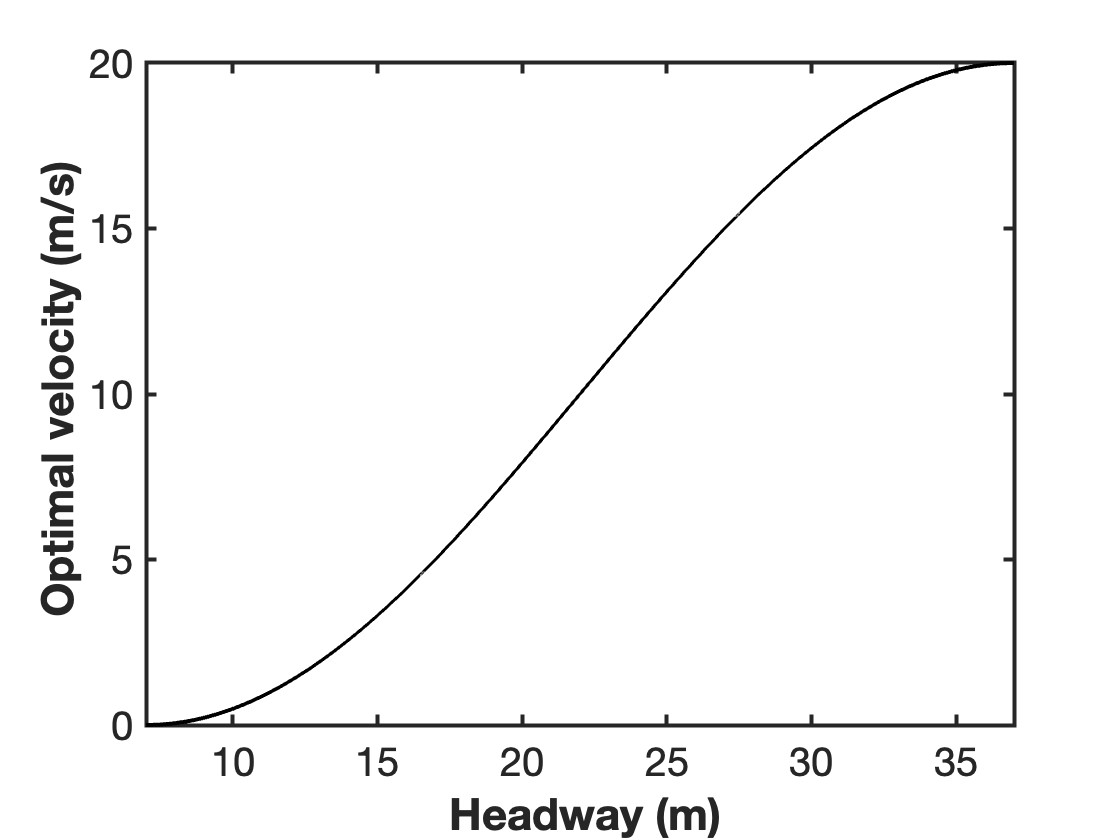
(a) Optimal velocity function

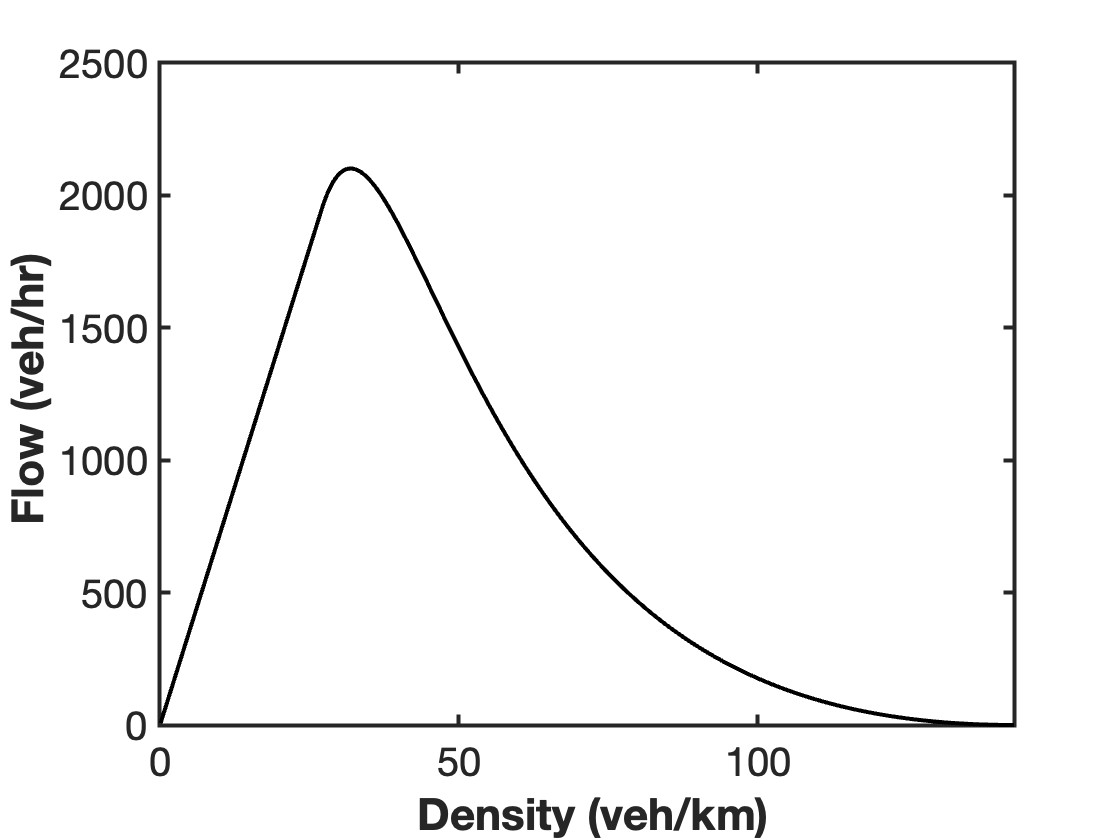
(b) Fundamental diagram

Figure 1: Plot of an optimal velocity function with $l=5$m and $v_{\max}=20$m/s and the corresponding fundamental diagram.

2.2 Platoon controller: A coordinated car following strategy

Now we consider a system of CAVs such that every following vehicle is connected to the leading autonomous vehicle. In other words, the following vehicles know the position and speed of the leading vehicle. In the proposed platoon model, we only use the position information of the leading vehicle and propose that the target (optimal) velocity of a following vehicle in the platoon is based on its distance from the leading vehicle:

$$\ddot{x}_{i}(t)=a\left[V(\frac{x_{N}(t)-x_{i}(t)}{N-i})-\dot{x}_{i}(t)\right]$$ (3)

where $x_{N}$ is the controlled leading vehicle. We refer (eq. 3) as the platoon controlled OVM (P-OVM) model. In this model, scaling is applied to the spacing between the leader of the platoon ($N$-th vehicle) and the $i$-th following vehicle used in the optimal velocity function, which is equivalent to consider the average spacing of vehicles between the leader of the platoon and the $i$-th following vehicle. Figure fig. 2 is an illustration of this platoon-controlled car-following configuration. Under this configuration, the influence of the immediate front vehicle is not taken into account, which could lead to collisions if the errors in position measurement and delays in communicaitons between the platoon leader and the following vehicles inside the platoon reach a certain level.

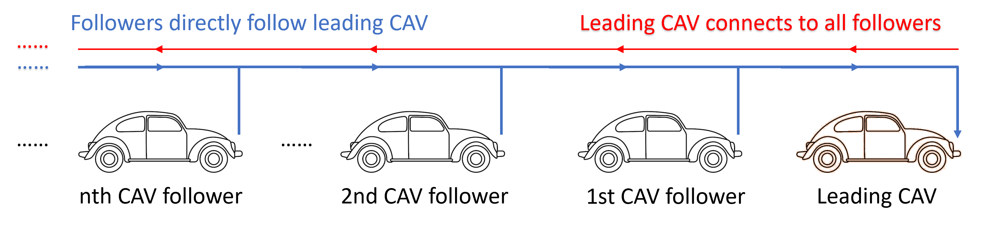
Figure 2: Illustration of the platoon-controlled car-following system. Leading CAV is connected to all followers of the platoon and followers are directly following the leading CAV

2.3 A transition phase model

We can address the previously mentioned safety issue by adding a local, within platoon vehicle-to-vehicle control to the P-OVM model. This local control can be any feedback control that eliminates vehicle collisions, and for the convenience of presentation and analysis, we adopt the OVM model as the local control model and called the combined model as the transition phase optimal velocity model (T-OVM). The model is of the form

$$\ddot{x}_{i}=a(V(x_{i+1}-x_{i})-\dot{x}_{i})+b\left(V\left(\frac{x_{N}-x_{i}}{N-i}\right)-\dot{x}_{i}\right)$$ (4)

where $a$ is the sensitivity to vehicle in front and $b$ is the sensitivity to the leading vehicle. The total sensitivity is defined as sum of the sensitivities $(a+b)$. Figure fig. 3 is an illustration of the car following pattern of T-OVM. With two parts of the model each vehicle inside the platoon will balance between the optimal velocity to the vehicle in front and the optimal velocity to the leading vehicle, to avoid collision and increase stability simultaneously.

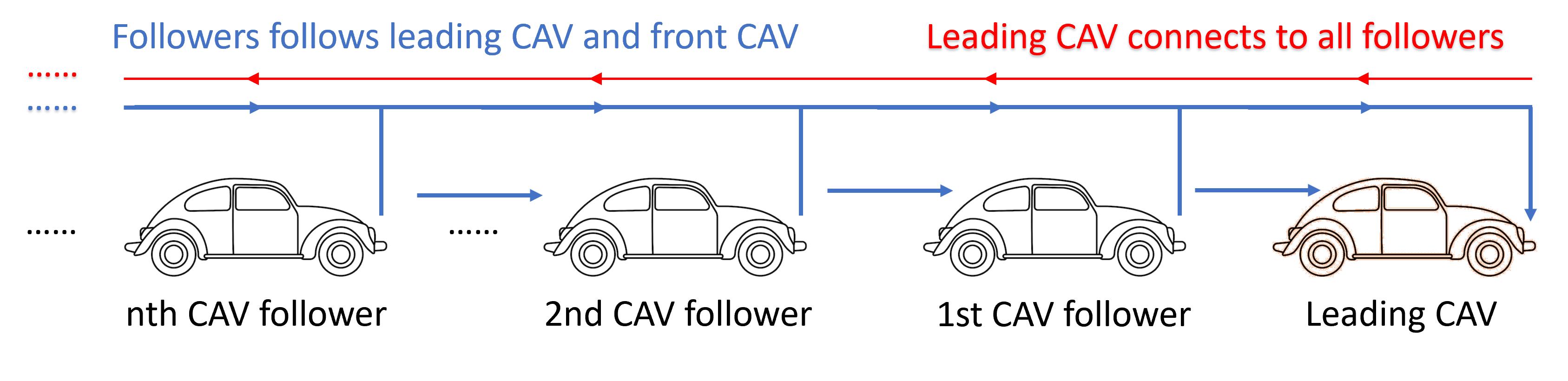
Figure 3: Illustration of the transition phase car-following system. Leading CAV is connected to all followers inside the platoon and followers are following the leading CAV and the front CAV simultaneously

3 Stability analysis of the platoon models

If the string of $N$ vehicles are on a ring road with length $L$ and the leading vehicle is following the last vehicle of the string by the original OVM (eq. 1), the position of $i-th$ vehicle is the same for both OVM (eq. 1) and P-OVM (eq. 5) under steady state:

$$e_{i}(t)=hi+V(h)t$$ (5)

where $h=L/N$ is the equilibrium headway. For the classic optimal velocity model, we have the following linear stability criterion:

Theorem 3.1.

The optimal velocity model (eq. 1) is linearly stable if

$$a>2V^{\prime}(h).$$ (6)

A proof slightly different from [4] is given in Appendix appendix A. Then with the platoon controller applied, it turns out that no stability criteria is required:

Theorem 3.2.

In the $N$-vehicle platoon where the leader vehilce follows the last vehicle of the platoon on a ring road according to OVM (eq. 1), the platoon-controlled system P-OVM (eq. 3) is always linearly stable.

Proof.

From previous introduction, P-OVM has the same equilibrium solution of the optimal velocity model as $x_{n}^{0}(t)=e_{n}(t)$ for any car $n$ inside the platoon. Now suppose that all the vehicles are deviated from the initial position with a small disturbance $y_{n}(t)$, that is,

$$x_{n}(t)=e_{n}(t)+y_{n}(t),\;|y_{n}|\ll 1$$ (7)

To linearize the original system, we can do a Taylor expansion of the optimal velocity function term $V(\Delta x_{n})$ and neglect the higher order terms to get

$$\ddot{y}_{n}(t)=\begin{cases}a\left[(V^{\prime}(h)\frac{y_{N}(t)-y_{n}(t)}{N-n}-\dot{y}_{n}(t)\right],\;\text{if }n\neq N\\ a\left[(V^{\prime}(h)(y_{1}(t)-y_{N}(t))-\dot{y}_{N}(t)\right],\;\text{if }n=N\end{cases}$$ (8)

Then by the formation of the controller, $y_{1}$ and $y_{N}$ forms a system of 2 linear ODEs, and the solution in vector form is:

$$\mathbf{Y}=\sum_{n=1,\;N}C_{n}e^{\lambda_{n}t}\mathbf{V}_{n}$$ (9)

Where $Y=[y_{1},y_{N}]^{T}$ is the vector form, $\lambda_{n}$ and $V_{n}$ are the eigenvalues and eigenvectors of the system, and $C_{n}$ are constants determined by the initial condition. Now suppose that $\lambda$ is an eigenvalue of the system, and $\xi_{n}$ is the coefficient of $y_{n}$ with the term $e^{\lambda t}$, then simplified from (eq. 8), $\lambda$ satisfies

$$\lambda^{2}+a\lambda-aV^{\prime}(h)(\frac{\xi_{1}}{\xi_{N}}-1)=0,$$ (10)

and

$$\lambda^{2}+a\lambda-aV^{\prime}(h)(\frac{\xi_{N}}{(N-1)\xi_{1}}-\frac{1}{N-1})=0$$ (11)

Then by comparing these equations we can calculate that $\xi_{1}=\xi_{N}$ or $\xi_{1}=-\xi_{N}/(N-1)$. And the first case is only true if we have $y_{1}=y_{N}$ and the two cars just stay at the same distance from the original equilibrium. For the other case we have

$$\lambda^{2}+a\lambda-aV^{\prime}(h)(-\frac{1}{N-1}-1)=0$$ (12)

Then, by solving the quadratic equation, we have

$$\lambda=\pm\frac{-a+\sqrt{a^{2}+4aV^{\prime}(h)(-\frac{1}{N-1}-1)})}{2}$$ (13)

For the system to be stable, we need to have the real parts of both $\lambda$ to be negative. This is true if $V^{\prime}(h)>0$ which is always true for any well-defined $V(h)$. Now we just need to check if the same property holds for the remaining vehicles. By (eq. 8) we can have a initial guess that the nonlinear part is $y_{j}=\zeta y_{N}$ for $j\neq 1$, then plug this into (eq. 8) and compare the coefficients we have

$$\zeta=N-j+\frac{j-1}{N-1}$$ (14)

Thus the other cars also have the same eigenvalue for the nonlinear part and the system will always be linearly stable if the problem is well defined. ∎

As for the transition phase model, stability clearly depends on both $a$, $b$ and $N$. For $N$ sufficiently large we have the following stability criterion:

Theorem 3.3.

Assuming that the leading vehicle follows the last vehicle by OVM (eq. 1) with sensitivity constant $a+b$. Then the transition phase model T-OVM (eq. 4) is linearly stable if

$$\frac{(a+b)^{2}}{a}>2V^{\prime}(h)$$ (15)

The proof is given in Appendix appendix B. Figure fig. 4 is a plot of neutral stability lines for different sensibilities and the area above the lines is the stable and below is unstable. And from this figure it is clear that with larger values of $b$ the unstable area is smaller and eventually vanished if $a\to 0$.

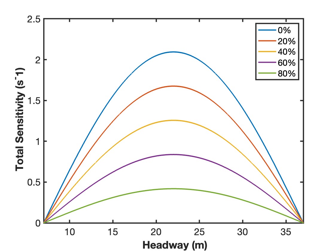
Figure 4: neutral stability lines of the transition phase model for selected percentages of leading vehicle sensitivity $b/(a+b)=0\%,20\%,40\%,60\%,80\%$. Above each line the region is stable and below is unstable.

4 Numerical simulation

To have a better visualization of how stability is improved by applying platoon control, several numerical experiments are conducted for different road settings and model parameters. All the numerical simulations are performed on MATLAB 2023b with simulation time step $\Delta t=0.1$s. To update solutions of each time step, forward Euler is applied for velocity variable $\dot{x}_{i}$ and a modified Euler scheme (Heun’s method) is applied for position variable $x_{i}$:

$$\dot{x}_{i,j+1}=\dot{x}_{i,j}+\ddot{x}_{i,j}\Delta t;\;x_{i,j+1}=x_{i,j}+\frac{\dot{x}_{i,j}+\dot{x}_{i,j+1}}{2}\Delta t$$ (16)

where $x_{i,j}$ is referring to the position of $i$-th car at $j$-th time step of simulation. This is equivalent to the discretizaiton method in [15].

4.1 Ring road with initial disturbance

In this subsection simulations are performed on a ring road. The total length of the ring road is $L=264$m with a total of 12 vehicles. As for model parameters we choose the optimal velocity function given by (eq. 2) and set $h_{\min}=7$m, $h_{\max}=37$m, $v_{\max}=20$m/s and $l=5$m. Then the equilibrium headway is $h=L/N=22$m and the equilibrium velocity is $V(h)=10$ m/s. The initial position and velocity of the $i$-th vehicle are deviated from the equilibrium states $(e_{i},V(h))$ with random perturbation uniformly distributed on the interval $[0,5]$. The initial condition of the model can be written as

$$\begin{cases}x_{i}(0)=&e_{i}(0)+r_{i},\\ \dot{x}_{i}(0)=&V(h)+\bar{r}_{i}\end{cases}$$ (17)

where $r_{i},\bar{r}_{i}$ are random numbers generated from uniform distribution on $[0,5]$, and $e_{i}(0)=hi$ can be calculated from (eq. 5).

Simulation 1.1: Comparison of OVM and P-OVM

To show the stability improvement of P-OVM, for sensitivity constant $a$, we tested for $a=0.4,\;0.8\;,1.6,\;2.4$ for both OVM and P-OVM with the same initial condition. Simulation results are shown for the original OVM and platoon-controlled OVM in Figures[fig. 5-fig. 8]. Figures [fig. 5, fig. 6] are the 3-D plots of headways of all vehicles under OVM and P-OVM with different values of $a$ respectively . Figures [fig. 7, fig. 8] are the velocity profiles of the $6$th vehicle under OVM and P-OVM respectively with different values of $a$.

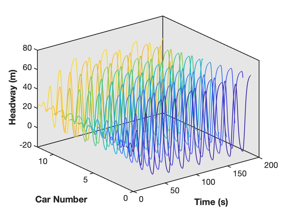
(a) $a=0.4$

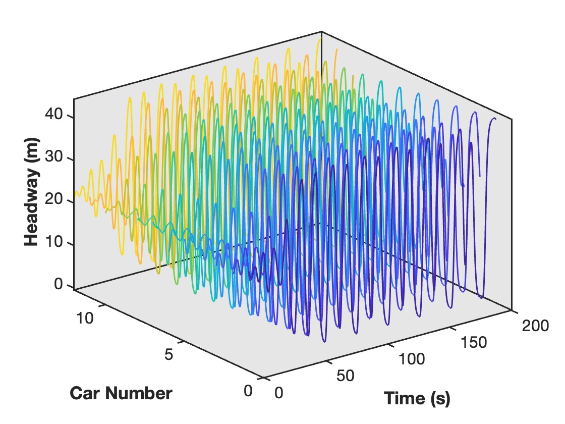
(b) $a=0.8$

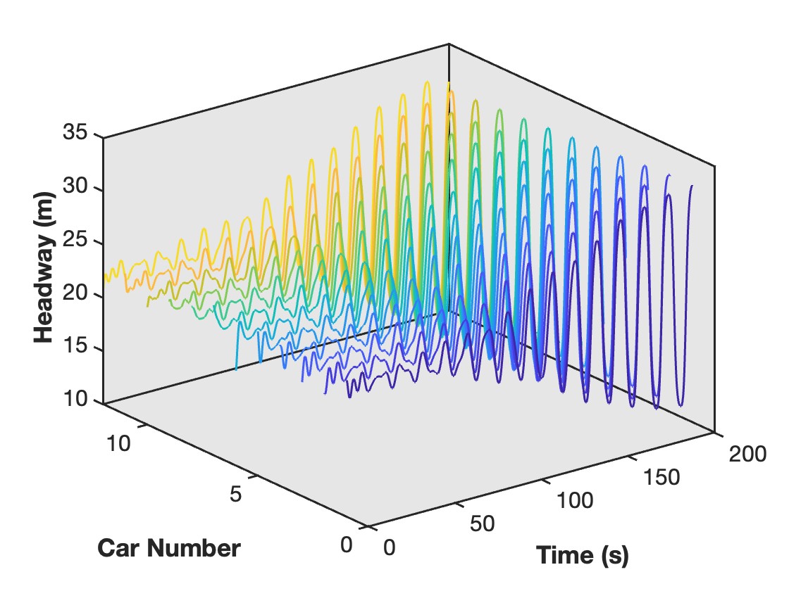
(c) $a=1.6$

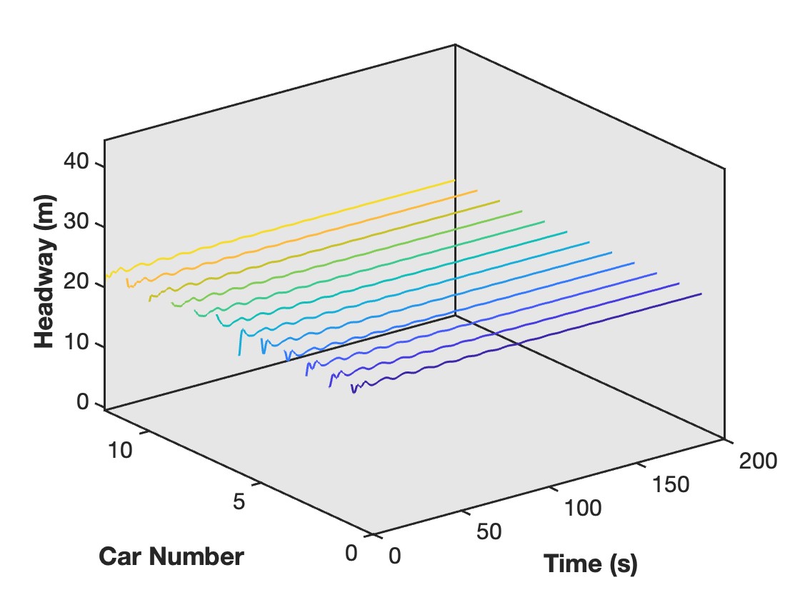
(d) $a=2.4$

Figure 5: Headway profile of OVM with sensitivity constant $a=0.4,\;0.8\;,1.6,\;2.4$

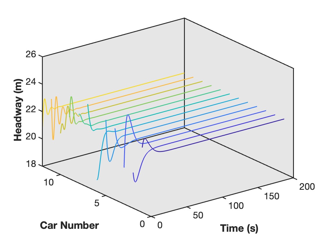
(a) $a=0.4$

(b) $a=0.8$

(c) $a=1.6$

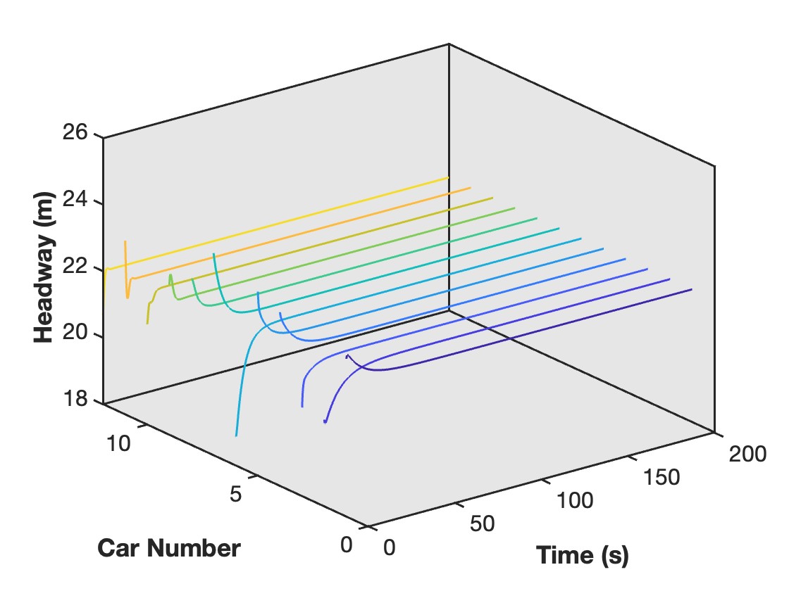
(d) $a=2.4$

Figure 6: Headway profile of P-OVM with sensitivity constant $a=0.4,\;0.8\;,1.6,\;2.4$

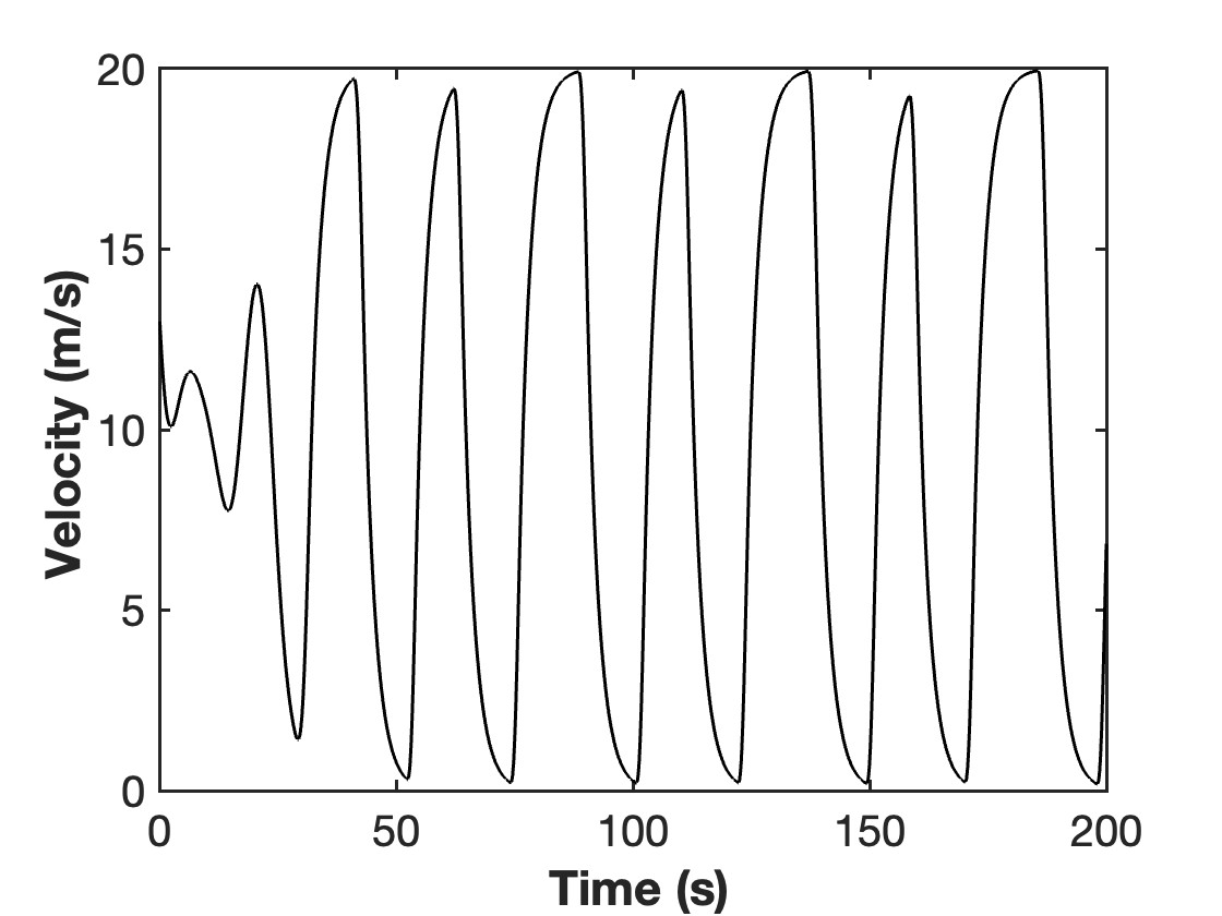
(a) $a=0.4$

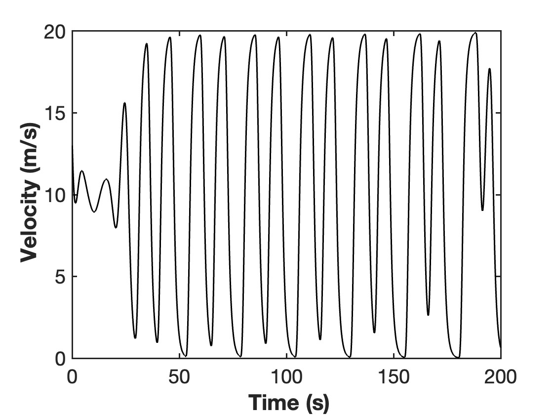
(b) $a=0.8$

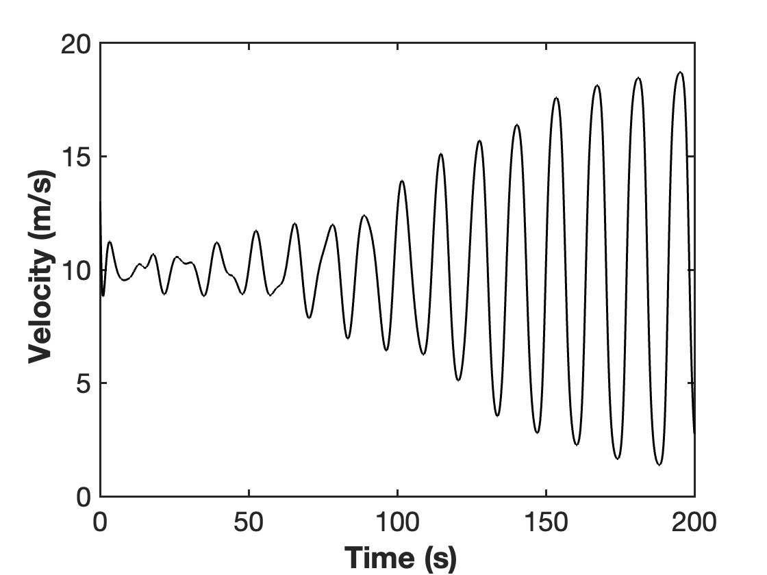
(c) $a=1.6$

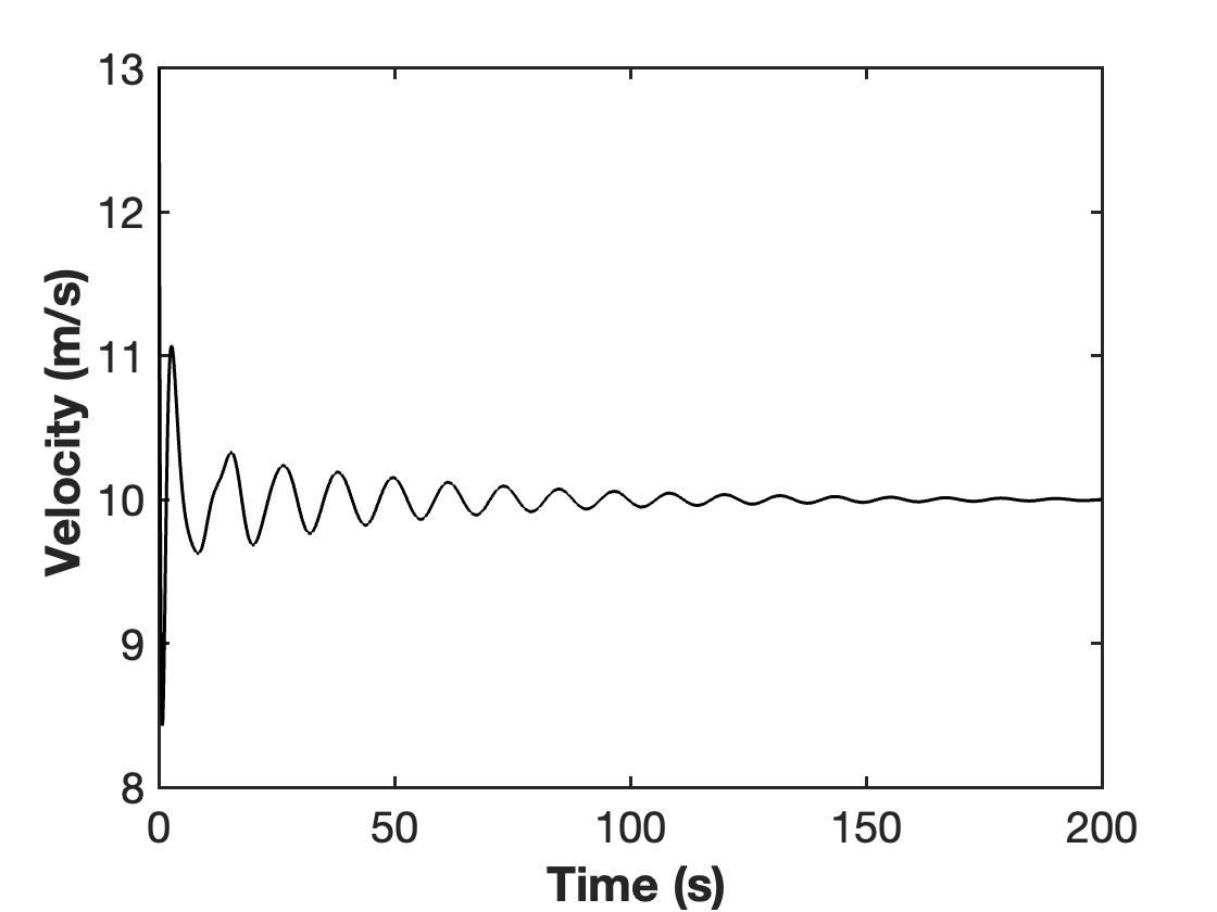
(d) $a=2.4$

Figure 7: Velocity profile of $6$th vehicle of OVM with sensitivity constant $a=0.4,\;0.8\;,1.6,\;2.4$

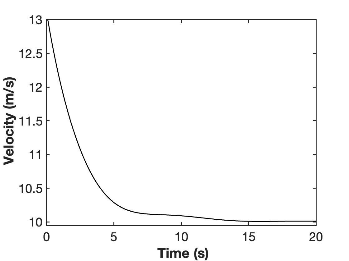
(a) $a=0.4$

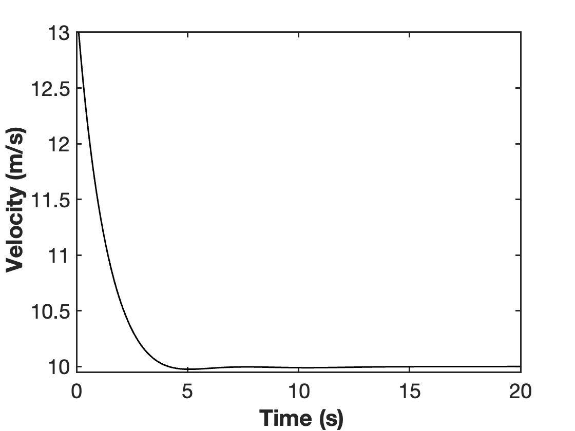
(b) $a=0.8$

(c) $a=1.6$

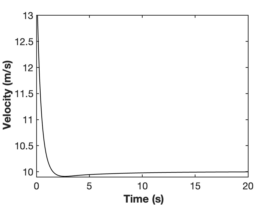
(d) $a=2.4$

Figure 8: Velocity profile of $6$th vehicle of P-OVM with sensitivity constant $a=0.4,\;0.8\;,1.6,\;2.4$

From the simulation results, for $a=0.4,\;0.8\;,1.6$ OVM is unstable. For $a=0.4$ negative headway can be generated which means collisions can happen with low sensitivity, and for $a=2.4$ OVM is stable but the initial acceleration is unrealistically large for the selected vehicle. As for P-OVM, for all selected values of $a$ the model is stable and $a$ is only affecting the convergence speed: for greater values of $a$ the flow converge to equilibrium state faster and for $a$ sufficiently large the improvement in convergence is minor since the original OVM is already stable.

Simulation 1.2: Test parameters of T-OVM

To test the performance of the transition phase model, four cases of sensitivity pair: $(a,b)=(0.5,0.1),$ $(0.1,0.5),$ $(1,0.2),$ $(0.6,0.6)$ are tested with same initial condition. Extreme cases of $a=0$ or $b=0$ are not considered since they are already presented in the previous section. Simulation results are in Figures [fig. 9-fig. 10]. Figure fig. 9 is the headway profile of all 12 vehicles in 3-D plot with different pairs of sensitivity constants and Figure fig. 10 is the velocity profile of the $6$th vehicle.

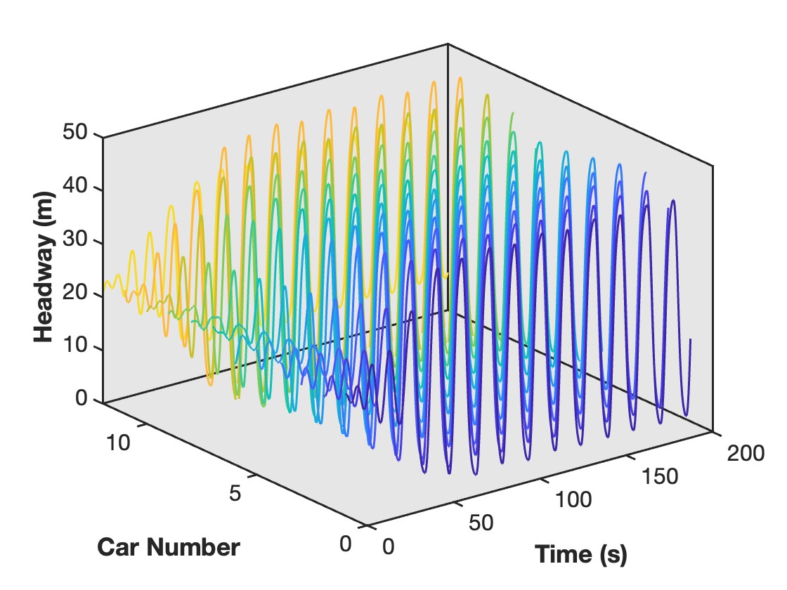
(a) $(a,b)=(0.5,0.1)$

(b) $(a,b)=(0.1,0.5)$

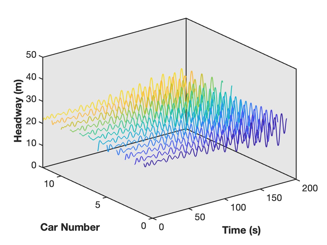
(c) $(a,b)=(1,0.2)$

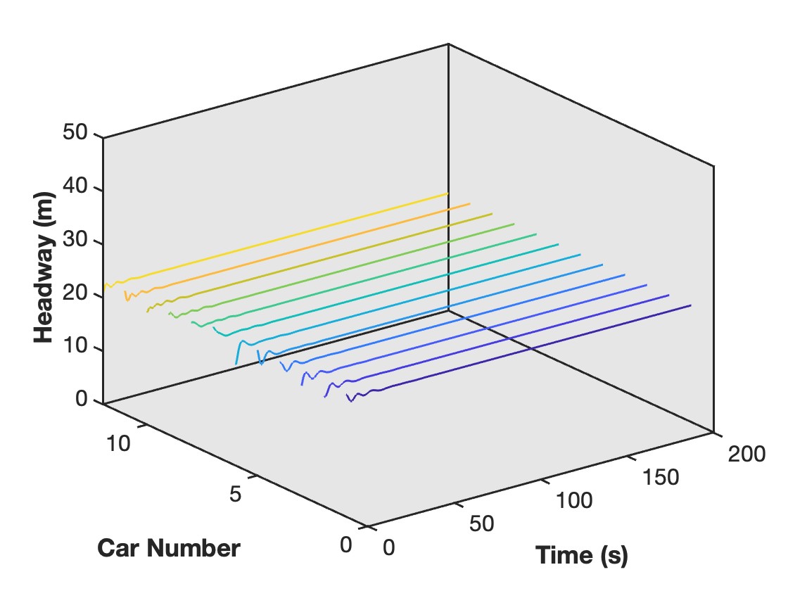
(d) $(a,b)=(0.6,0.6)$

Figure 9: Headway profile of T-OVM with sensitivity constant $(a,b)=(0.5,0.1),(0.1,0.5),(1,0.2),(0.6,0.6)$

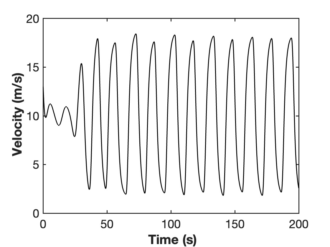
(a) $(a,b)=(0.5,0.1)$

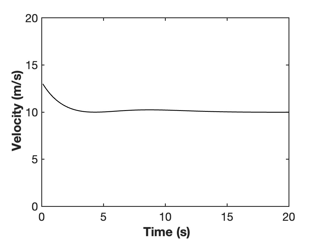
(b) $(a,b)=(0.1,0.5)$

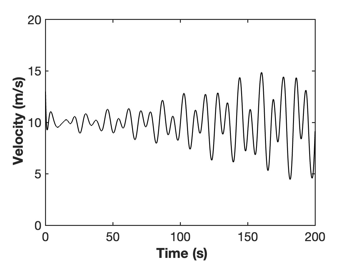
(c) $(a,b)=(1,0.2)$

(d) $(a,b)=(0.6,0.6)$

Figure 10: Velocity profile of $6$th vehicle of T-OVM with sensitivity constant $(a,b)=(0.5,0.1),(0.1,0.5),(1,0.2),(0.6,0.6)$

From the simulation results, we can see that with the increase of percentage of leading vehicle sensitivity, the traffic stream is more stable. And for higher total sensitivity $(a+b)$ less percentage of leading vehicle sensitivity is required, which is consistent with theoretical results (see figure fig. 4). Moreover, OVM and P-OVM can be considered as extreme cases of T-OVM.

Simulation 1.3: Compare T-OVM and with two cars ahead following

To show the effectiveness of following the leader of platoon, we compare T-OVM (eq. 4) with the front multi-following OVM (F-OVM) of two cars in [7]:

$$\ddot{x}_{i}=a(V(x_{i+1}-x_{i})-\dot{x}_{i})+b\left(V\left(\frac{x_{i+2}-x_{i}}{2}\right)-\dot{x}_{i}\right)$$ (18)

where the sensitivity $b$ is for the second vehicle in front. Two cases of sensitivity pair: $(a,b)=(0.8,0.4),(0.2,0.4)$ are tested. Simulation results are in Figures fig. 11, fig. 12. Figure fig. 11 is the headway profile of all 12 vehicles in 3-D plot with T-OVM and F-OVM and Figure fig. 12 is the velocity profile of the $6$th vehicle.

(a) T-OVM with $(a,b)=(0.8,0.4)$

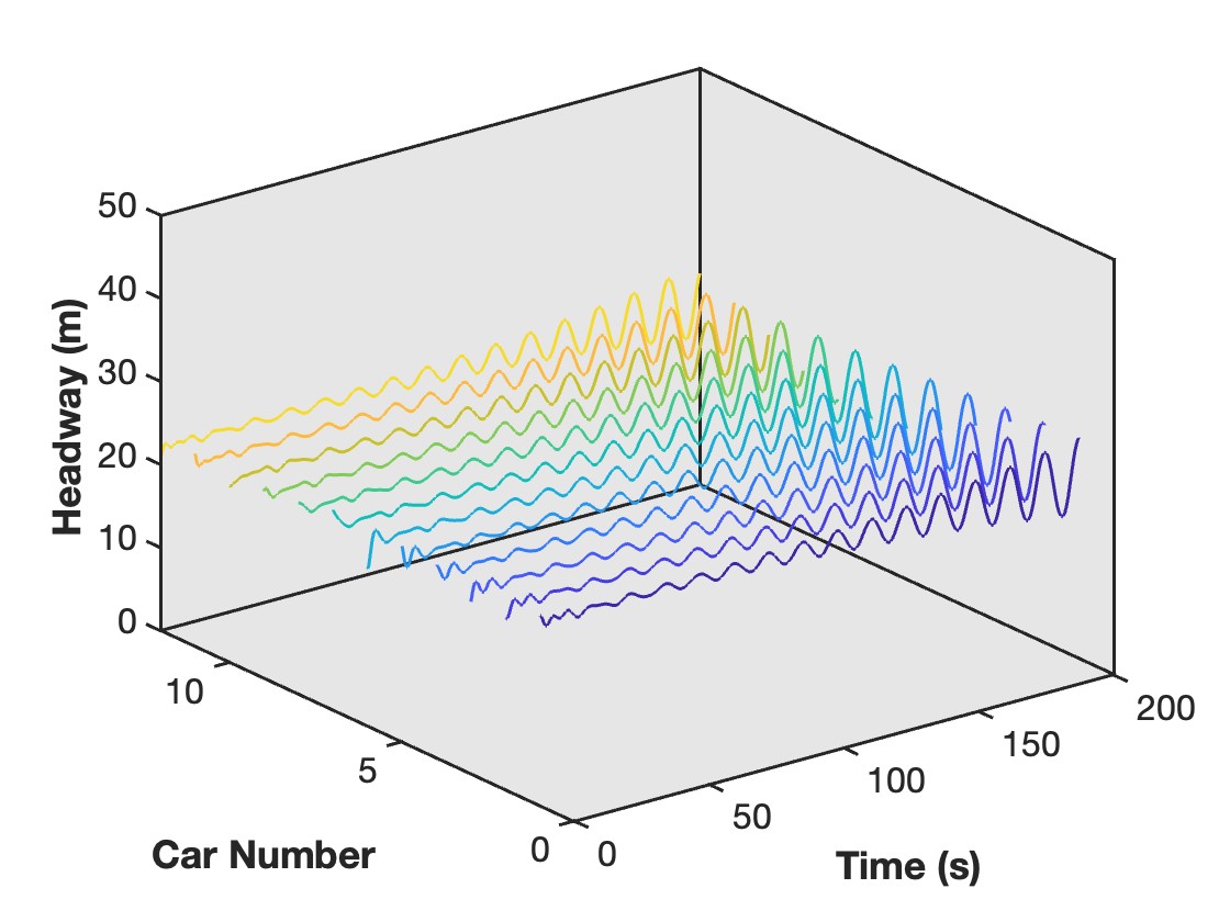
(b) F-OVM with $(a,b)=(0.8,0.4)$

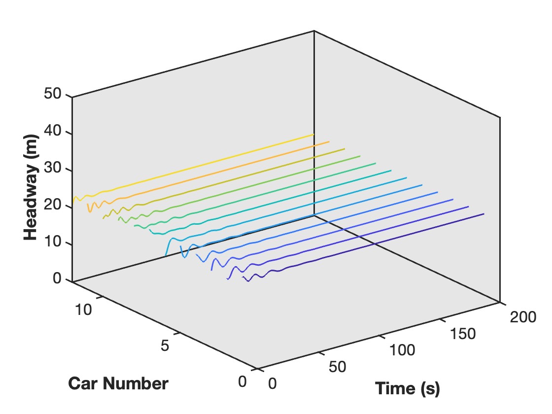
(c) T-OVM with $(a,b)=(0.2,0.4)$

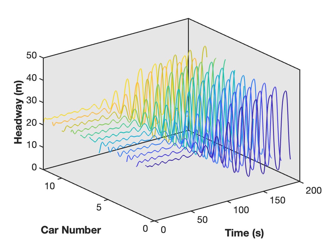
(d) F-OVM with $(a,b)=(0.2,0.4)$

Figure 11: Headway profile of T-OVM and F-OVM with sensitivity constant $(a,b)=(0.8,0.4),(0.2,0.4)$

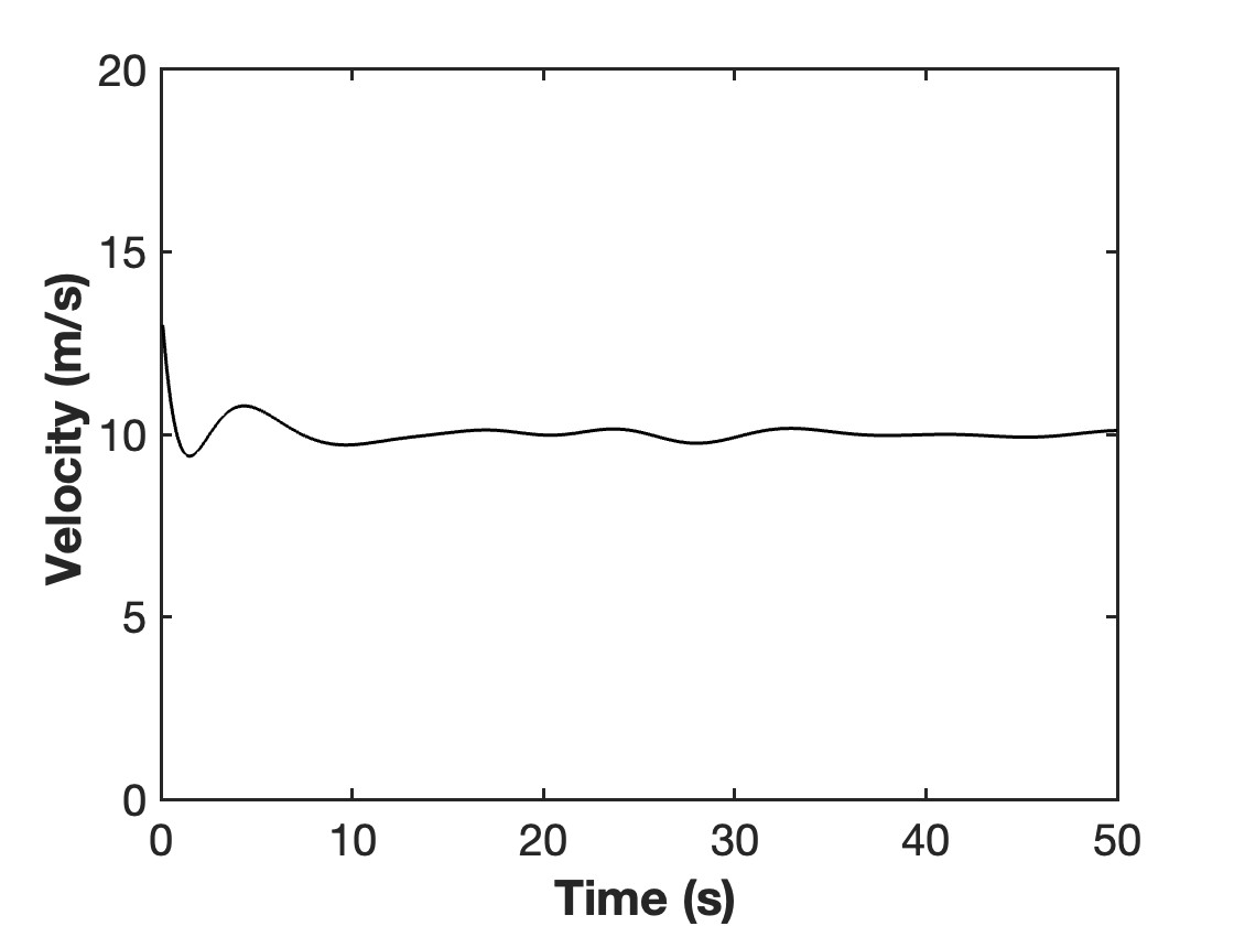
(a) T-OVM with $(a,b)=(0.8,0.4)$

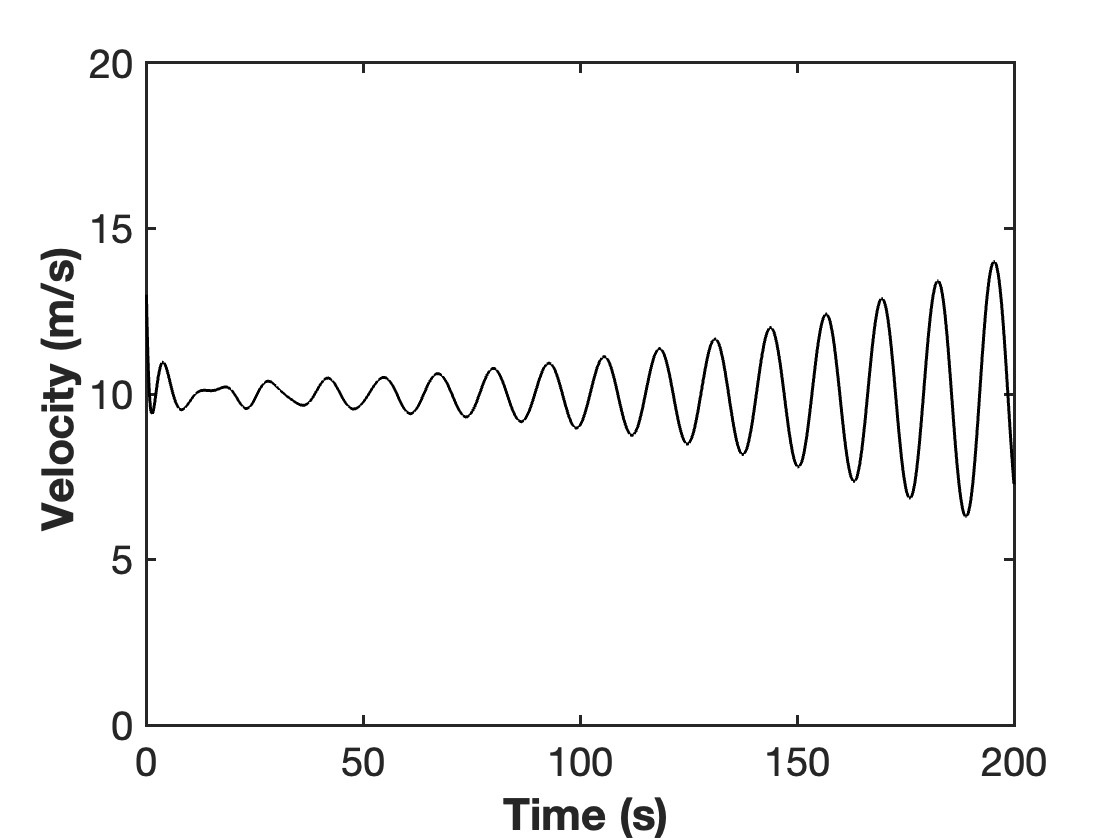
(b) F-OVM with $(a,b)=(0.8,0.4)$

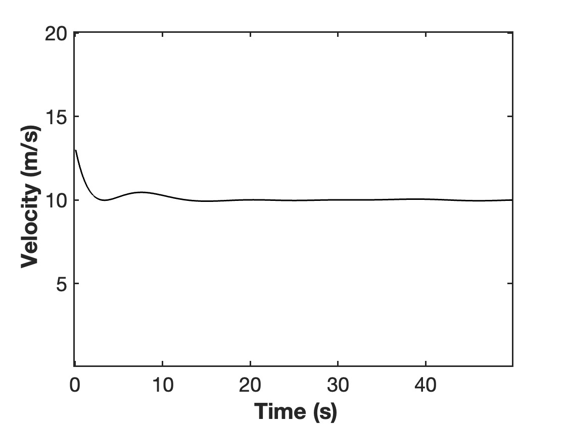
(c) T-OVM with $(a,b)=(0.2,0.4)$

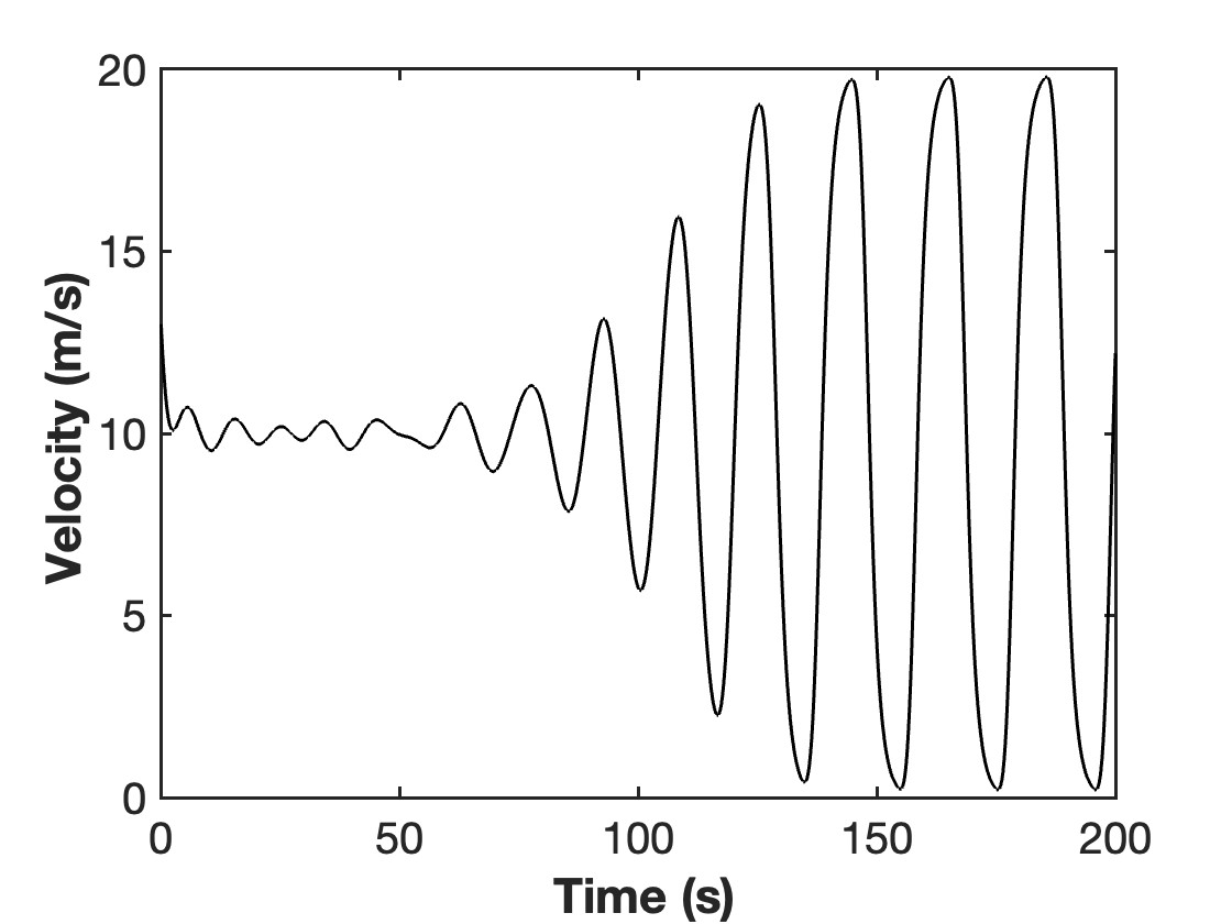
(d) F-OVM with $(a,b)=(0.2,0.4)$

Figure 12: Velocity profile of $6$th vehicle of T-OVM and F-OVM with sensitivity constant $(a,b)=(0.8,0.4),(0.2,0.4)$

From the simulation results we can see that for same set of sensitivity parameters, T-OVM can suppress the disturbance and the platoon remians stable while F-OVM cannot. Moreover, this stabilizing effect of T-OVM becomes more prominent when the following vehicles repond more strongly to the leader in T-OVM, while the destabilizing effect in the F-OVM becomes stronger when the following vehicle respond more strongly to the two-vehicle ahead vehicle, demonstrating the superiority of T-OVM in stabilizing vehicle platoons.

4.2 Infinite road with periodic disturbance

Other than initial disturbance, it is interesting to know if platoon control can also increase stability under periodic disturbance. Suppose that a total of $N=10$ vehicles are on a infinite road with free flow speed $v_{max}=30$m/s and uniform length $l=5$m. The optimal velocity function $V_{I}(h)$ for the infinite road simulation is equivalent to triangular fundamental diagram:

$$V_{I}(h)=\begin{cases}v_{\max},&\text{if }\rho(h)\leq\rho_{c}\\ \frac{v_{\max}*\rho_{c}(\rho(h)-\rho_{\max})}{\rho(h)(\rho_{c}-\rho_{\max})},&\text{if }\rho_{c}\leq\rho(h)\leq\rho_{\max}\\ 0,&\text{if }\rho\geq\rho_{\max}\end{cases}$$ (19)

where $\rho(h)=l/h$ is the occupancy of vehicles on the road: $\rho=0$ means no vehicles and $\rho=1$ means full of vehicles. $\rho_{c}=5/37$ is the critical occupancy such that flow is maximized and $\rho_{\max}=5/7$ is the jam occupancy with $0$ speed. Figure fig. 13 is a plot of the optimal velocity function and corresponding triangular fundamental diagram.

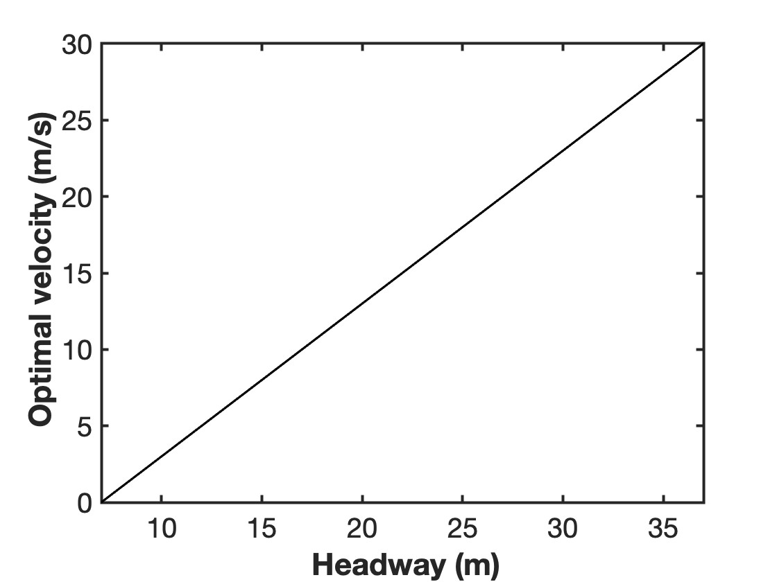
(a) Optimal velocity function

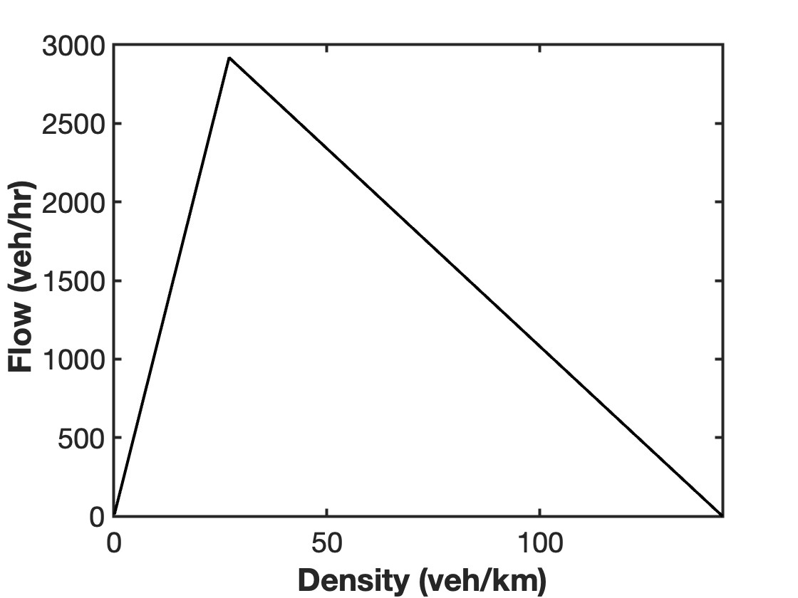
(b) Triangular fundamental diagram

Figure 13: Plot of an optimal velocity function with $l=5$m and $v_{\max}=30$m/s and the corresponding triangular fundamental diagram.

During the simulation time, the leading vehicle was trying to maintain at a given equilibrium speed but encountered sinusoidal disturbance, similar to [20]. The equilibrium speed is $v_{0}=15$m/s and the equilibrium headway is $h=29.5$m. And if we denote $p$ as duration of each period of the sinusoidal disturbance and $A$ as the amplitude of the disturbance, then the velocity of the leading vehicle can be written as:

$$v_{N}=v_{0}+A\sin\left(\frac{2\pi}{p}t\right)$$ (20)

where period duration $p=5,\;10,\;20,\;30$s and amplitude $A=5$m/s. OVM and P-OVM with sensitivity constant $a=1.2,\;2.4$ are tested. The simulation duration is $60$ seconds for all simulations. Simulation results are in Figure [fig. 14-fig. 17]. Figure fig. 14, fig. 15 are the headway profiles of OVM and P-OVM with sensitivity constant $a=1$ under different perturbation frequency. Figure fig. 16, fig. 17 are the headway profiles of OVM and P-OVM with sensitivity constant $a=2$ under different perturbation frequency.

(a) $p=20$

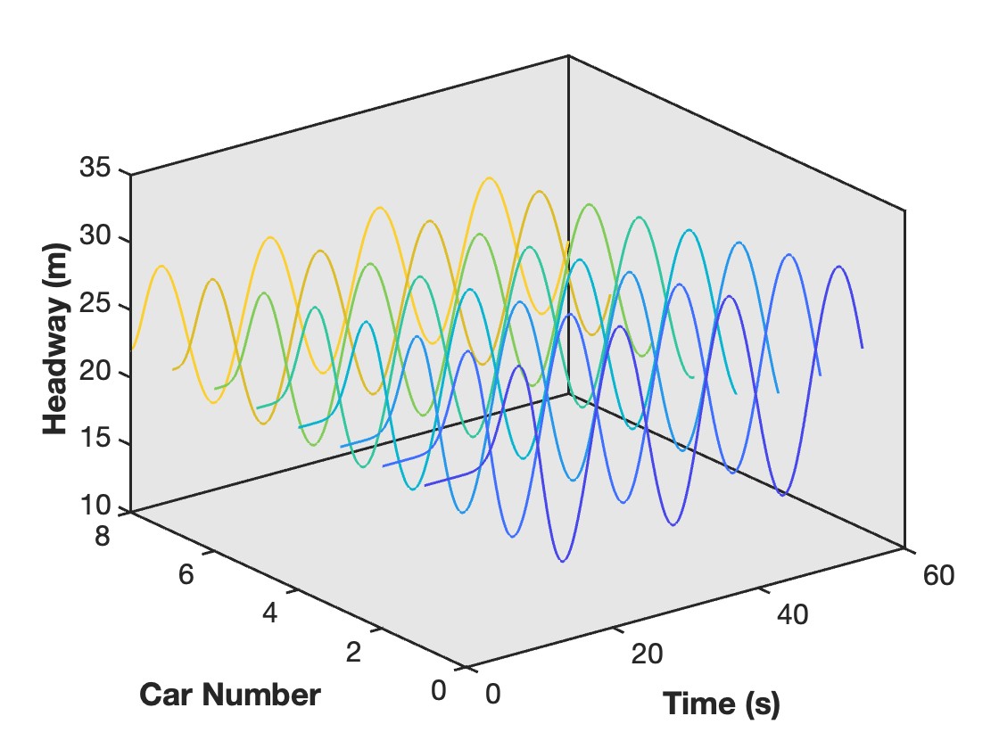
(b) $p=15$

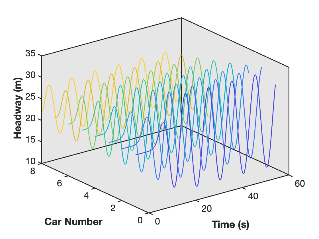
(c) $p=10$

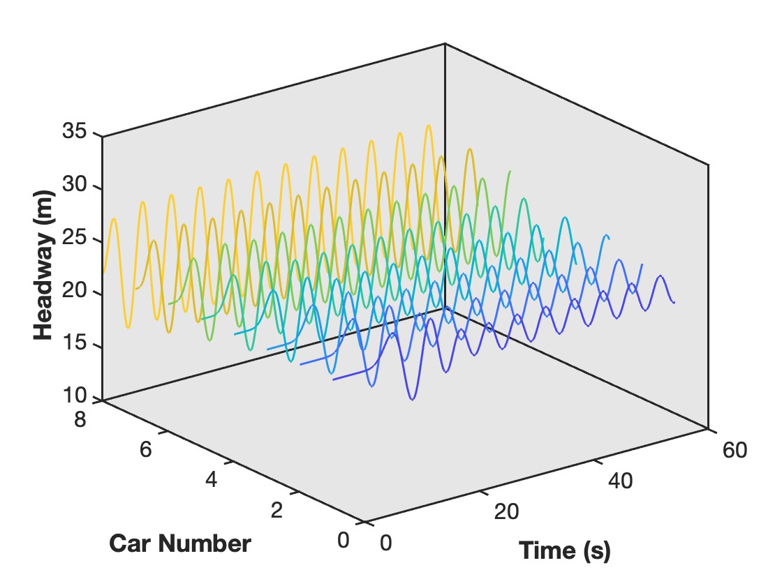
(d) $p=5$

Figure 14: Headway profile of OVM with sensitivity constant $a=1.2$ and period parameter $p=5,\;10,\;20,\;30$

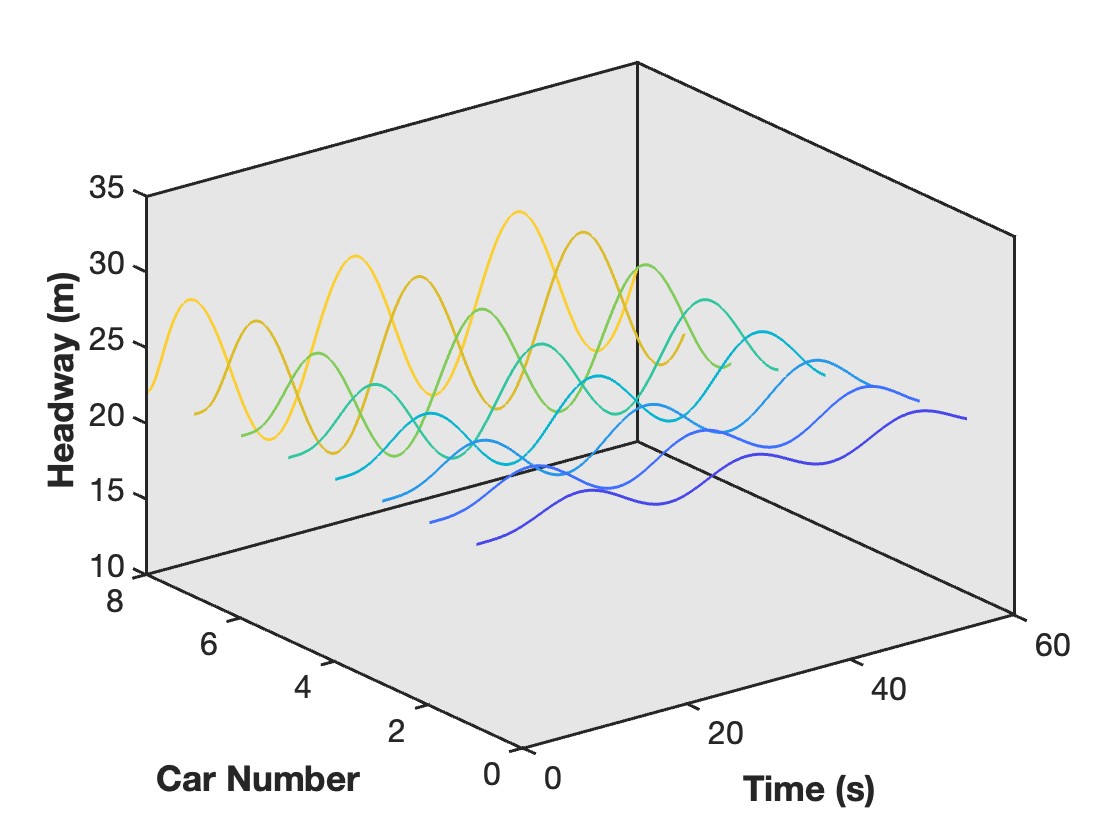
(a) $p=20$

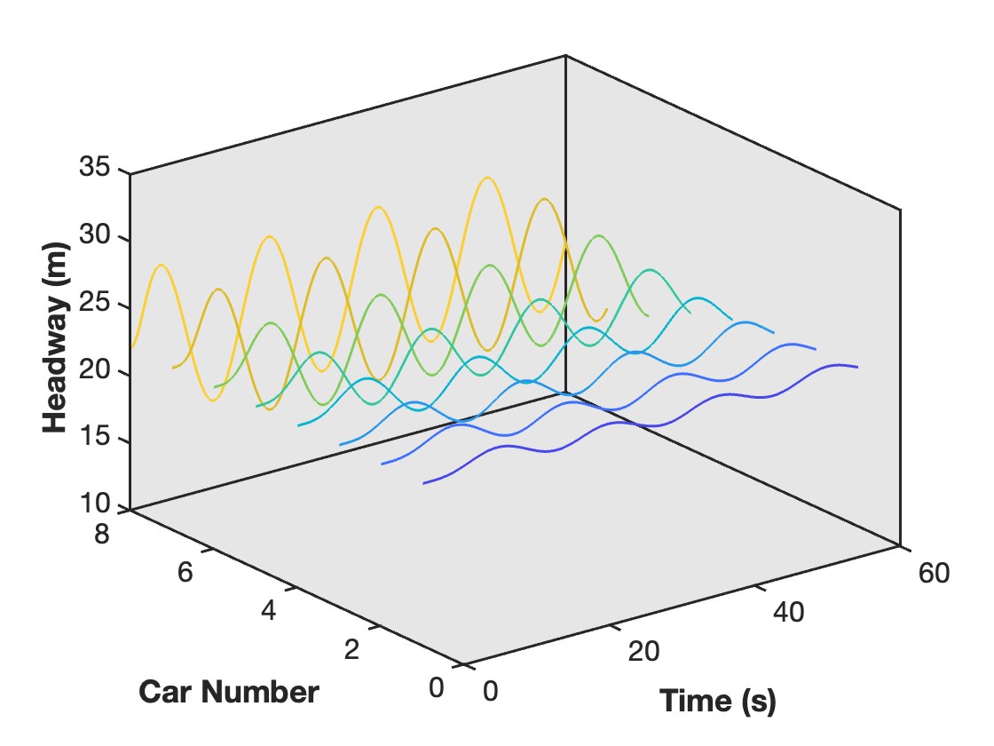
(b) $p=15$

(c) $p=10$

(d) $p=5$

Figure 15: Headway profile of P-OVM with sensitivity constant $a=1.2$ and period parameter $p=5,\;10,\;20,\;30$

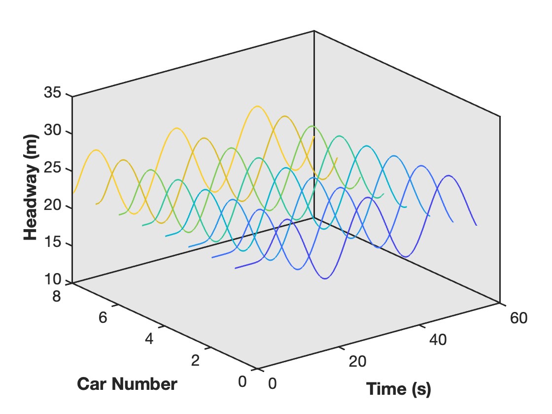
(a) $p=20$

(b) $p=15$

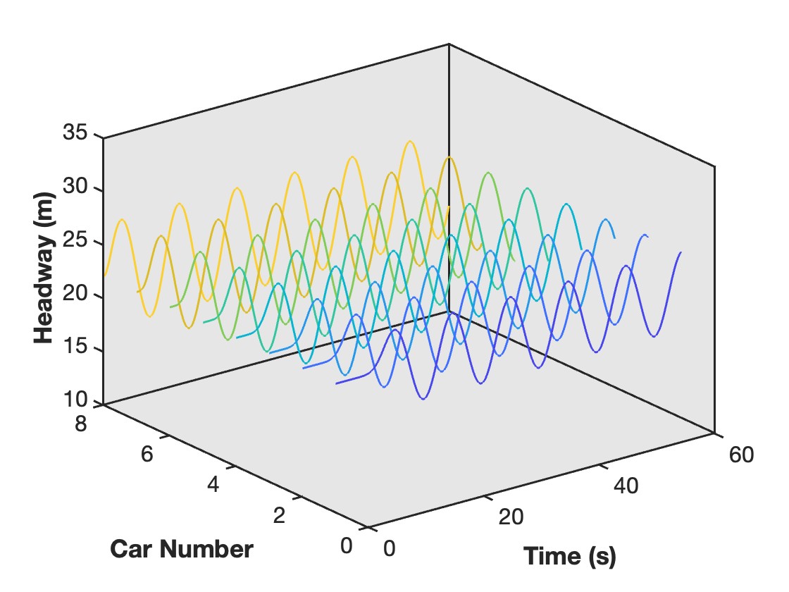
(c) $p=10$

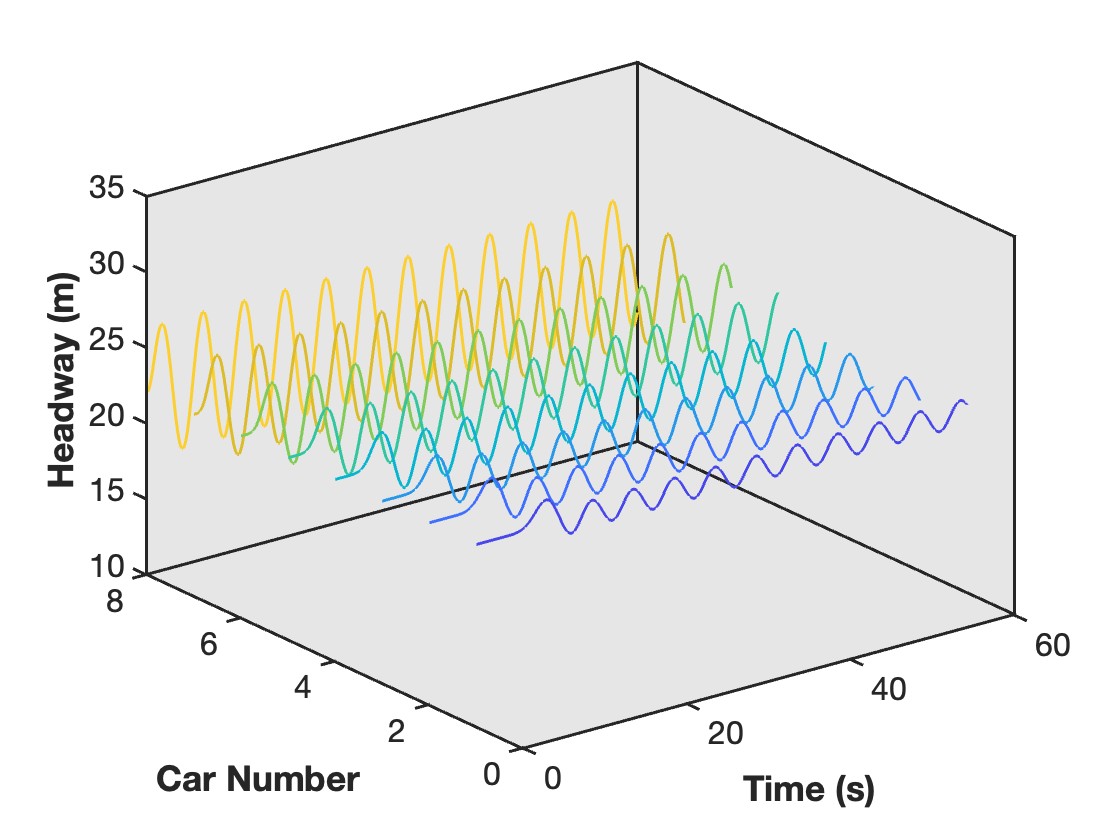
(d) $p=5$

Figure 16: Headway profile of OVM with sensitivity constant $a=2.4$ and period parameter $p=5,\;10,\;20,\;30$

(a) $p=20$

(b) $p=15$

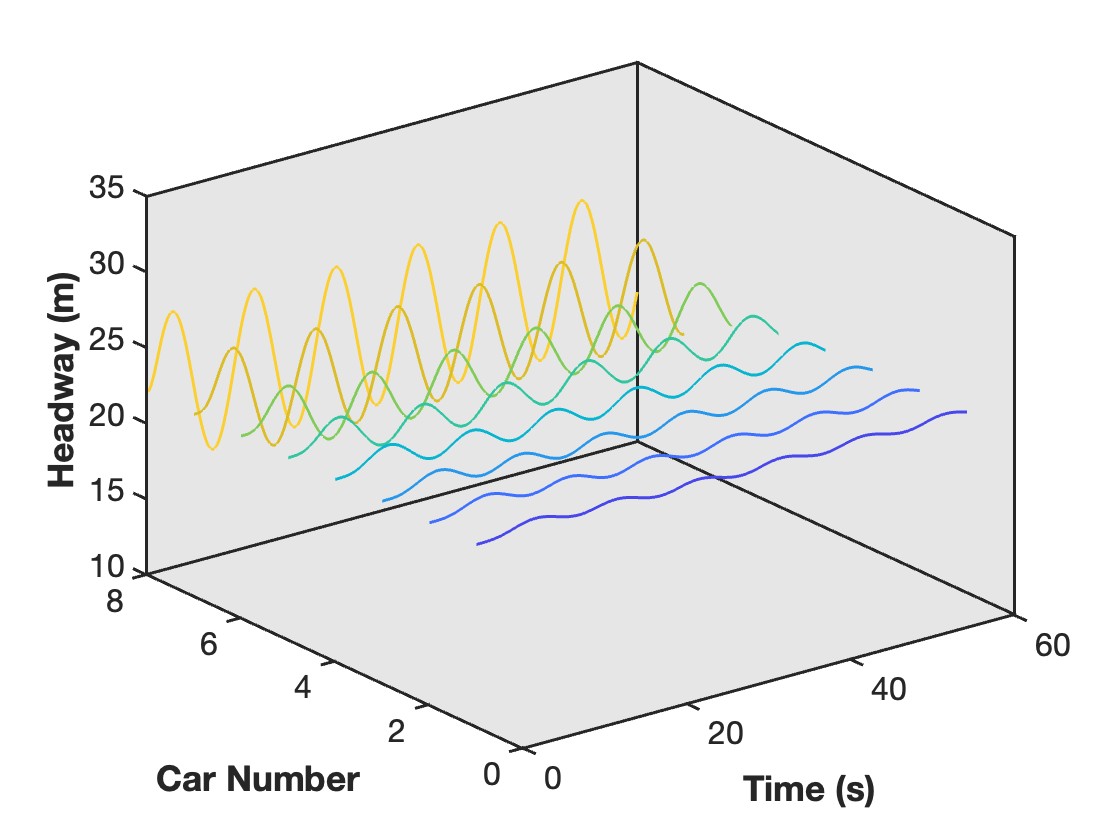
(c) $p=10$

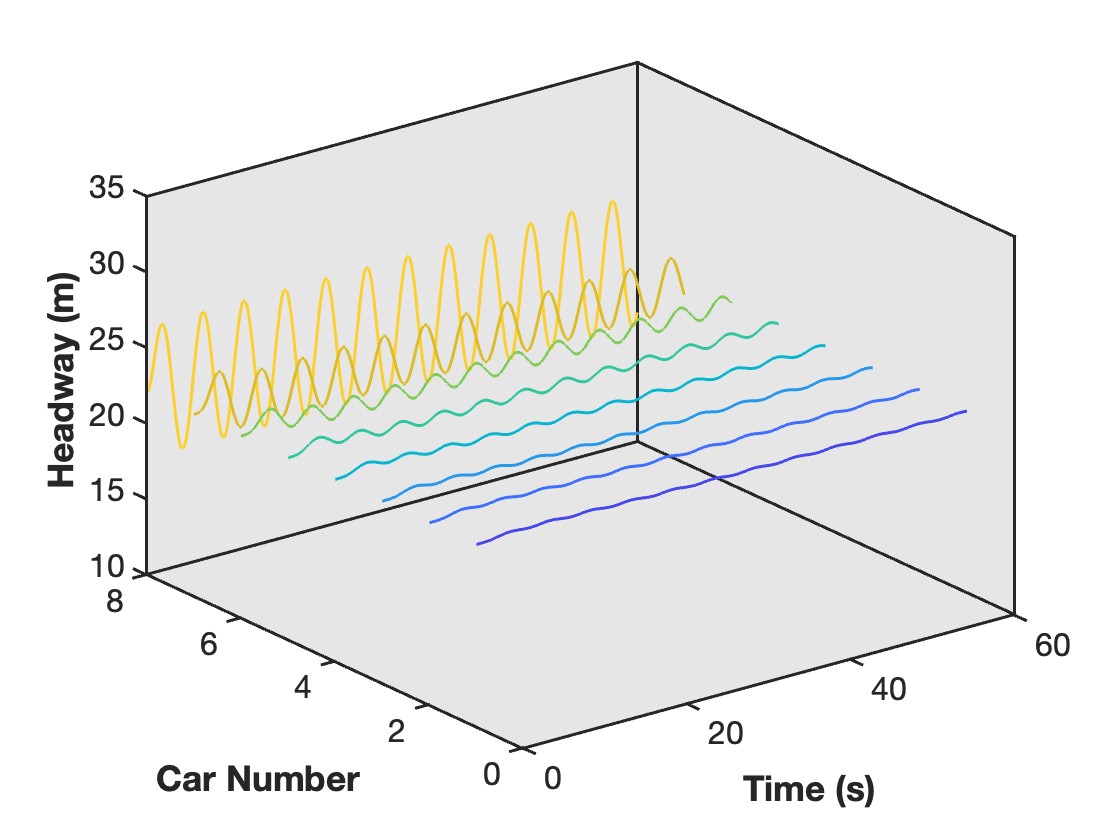
(d) $p=5$

Figure 17: Headway profile of P-OVM with sensitivity constant $a=2.4$ and period parameter $p=5,\;10,\;20,\;30$

From the simulation results, we can see that if the frequency of the sinusoidal disturbance is too high ($p=5$), the amplitude of disturbance can get smaller without applying platoon-control even when OVM is not stable ($a=1.2$), due to the frequent change of optimal velocity and the delayed reaction property of OVM. With platoon-controller applied, headway is stabilized around equilibrium state for all model parameters and have better stability when OVM is stable ($a=2.4$). In one sentence, P-OVM can increase string stability under periodic disturbance.

5 Conclusions

In this paper, a platoon model with coordinated following strategy (P-OVM) and a transition phase model with adjustable parameters (T-OVM) are proposed. P-OVM model is proved always linearly stable but the model has a limited practical use due to safety considerations when both the control and state measurements are subject to errors. Stability of the base model and transition phase model are also analysed and stability conditions for both models are provided. To verify the theoretical results, numerical simulations are performed on a ring road with an initial disturbance and an infinite road with a periodic disturbance. Multiple model parameters are tested and analysed. Results of the numerical simulations showed that with the proposed platoon control applied, linear stability is guaranteed for all sensitivity constants. The constants themselves just determine how quickly the disturbance is attenuated through the platoon. With the transition phase model for fixed total sensitivity, stability increases with sensitivity to the leading vehicle, which is consistent with theoretical analysis.

The proposed P-OVM and T-OVM models produce considerably better results in suppressing disturbances and maintaining string stability compared to non-controlled model OVM. These models are simple forms of platooning that multi-following models tend to focus on. This is a significant improvement compared to previous studies on multi-following models. With the fast development of CAV related technologies, the proposed platoon control offers a promising way to mitigate oscillations in traffic flow.

This paper can be extended in various directions for future research, including: (1) Add communication delay to the proposed models and analyse their impact on stability; (2) Consider more general road conditions, e.g. multi-lane ring road with mixed CAVs and HDVs. For such scenarios the control design of leading vehicle will be adjusted accordingly [18]; (3) Conduct field experiments with CAVs to test the control design under various traffic and road conditions.

Declaration of competing interest

The authors declare that there are no source of financial interests or personal relationships that could have any impacts of the work in this paper.

Appendix A Proof of Theorem eq. 6

In this section we give the proof of Theorem eq. 6:

Proof.

Similar to proof of Theorem theorem 3.2, we consider small deviation $y_{i}$ from the equilibrium solution and neglect higher order. Then we have

$$\ddot{y}_{i}(t)=a\left[(V^{\prime}(h)(y_{i+1}(t)-y_{i}(t))-\dot{y}_{i}(t)\right],\;y_{N+1}=y_{1}$$ (21)

which is a linear ODE system with $N$ equations. Suppose that $\lambda$ is an eigenvalue of the system, and $\xi_{i}$ is the coefficient of $y_{i}$ with the term $e^{\lambda t}$, then simplified from (eq. 21), $\lambda$ satisfies

$$\lambda^{2}+a\lambda-aV^{\prime}(h)(\frac{\xi_{i+1}}{\xi_{i}}-1)=0$$ (22)

This means $\xi_{i+1}/\xi_{i}=r$ is fixed for given $\lambda$, and note that $\prod_{i=1}^{N}(\xi_{i+1}/\xi_{i})=1$, we have

$$r=e^{\frac{2\pi k}{N}i},\;k=1,2,\dots,N$$ (23)

Therefore $\lambda$ satisfies

$$\lambda^{2}+a\lambda-aV^{\prime}(h)(e^{\frac{2\pi k}{N}i}-1)=0$$ (24)

for some $k=1,2,\dots,N$. Then, to have a stable system of $y_{n}$, the real parts of any $\lambda$ should be negative. By considering the solution of $\lambda$ with smaller real parts we have

$$\frac{a-\sqrt{d+\sqrt{d^{2}+e^{2}}}}{2}<0,$$ (25)

where $d=a^{2}+4aV^{\prime}(h)\cos\frac{2\pi k}{N}-4aV^{\prime}(h)$ and $e=-4aV^{\prime}(h)\sin\frac{2\pi k}{N}$. For the system to be stable, we need this condition to be satisfied for every $k$. Now let $\theta\triangleq\frac{2\pi k}{N}$ then (eq. 25) can be simplified to

$$-V^{\prime}(h)\cos^{2}\theta+a\cos\theta+V^{\prime}(h)-a<0$$ (26)

(eq. 26) holds if (eq. 6) holds, otherwise for N sufficiently large we can let $\cos\theta=a/2V^{\prime}(h)$ and (eq. 26) will fail. ∎

Appendix B Proof of Theorem eq. 15

In this section we give the proof of Theorem eq. 15:

Proof.

Again we consider small deviation $y_{i}$ from the equilibrium solution and neglect higher order. Then we have

$$\ddot{y}_{i}(t)=\begin{cases}a\left[V^{\prime}(h)(y_{i+1}(t)-y_{i}(t))-\dot{y}_{i}(t)\right]+b\left[V^{\prime}(h)\frac{y_{N}(t)-y_{i}(t)}{N-i}-\dot{y}_{i}(t)\right],\;\text{if }i\neq N\\ (a+b)\left[V^{\prime}(h)(y_{i+1}(t)-y_{i}(t))-\dot{y}_{i}(t)\right],\;\text{if }i=N\end{cases}$$ (27)

which is a linear ODE system with $N$ equations. Suppose that $\lambda$ is an eigenvalue of the system, and $\xi_{i}$ is the coefficient of $y_{i}$ with the term $e^{\lambda t}$, then simplified from (eq. 27), $\lambda$ satisfies

$$\lambda^{2}+(a+b)\lambda-aV^{\prime}(h)(\frac{\xi_{i+1}}{\xi_{i}}-1)-\frac{bV^{\prime}(h)}{N-i}(\frac{\xi_{N}}{\xi_{i}}-1)=0,\;\text{if }i\neq N$$ (28)

and

$$\lambda^{2}+(a+b)\lambda-(a+b)V^{\prime}(h)(\frac{\xi_{1}}{\xi_{N}}-1)=0$$ (29)

When N is very large ($N\to\infty$), $bV^{\prime}(h)/(N-i)$ is very small for most i, and the last term of (eq. 28) has minimal effect. This means $\xi_{i+1}/\xi_{i}$ will converge to eigenvalues given in (eq. 23). Then $\lambda$ will converge to values given by

$$\lambda^{2}+(a+b)\lambda-aV^{\prime}(h)(e^{\frac{2\pi k}{N}i}-1)=0$$ (30)

Follow the same steps of previous proof we can find the stability criterion (eq. 15). A more rigorous mathematical proof will be part of future work. ∎

References

- [1] Shahab Sheikholeslam and Charles A Desoer. Longitudinal control of a platoon of vehicles. In 1990 American control conference, pages 291–296. IEEE, 1990.
- [2] Louis A Pipes. An operational analysis of traffic dynamics. Journal of applied physics, 24(3):274–281, 1953.
- [3] Denos C Gazis, Robert Herman, and Richard W Rothery. Nonlinear follow-the-leader models of traffic flow. Operations research, 9(4):545–567, 1961.
- [4] Masako Bando, Katsuya Hasebe, Akihiro Nakayama, Akihiro Shibata, and Yuki Sugiyama. Dynamical model of traffic congestion and numerical simulation. Physical review E, 51(2):1035, 1995.
- [5] Masako Bando, Katsuya Hasebe, Ken Nakanishi, Akihiro Nakayama, Akihiro Shibata, and Yūki Sugiyama. Phenomenological study of dynamical model of traffic flow. Journal de Physique I, 5(11):1389–1399, 1995.
- [6] Martin Treiber, Ansgar Hennecke, and Dirk Helbing. Congested traffic states in empirical observations and microscopic simulations. Physical review E, 62(2):1805, 2000.
- [7] H Lenz, CK Wagner, and R Sollacher. Multi-anticipative car-following model. The European Physical Journal B-Condensed Matter and Complex Systems, 7:331–335, 1999.
- [8] Akihiro Nakayama, Yūki Sugiyama, and Katsuya Hasebe. Effect of looking at the car that follows in an optimal velocity model of traffic flow. Physical Review E, 65(1):016112, 2001.
- [9] Rui Jiang, Qingsong Wu, and Zuojin Zhu. Full velocity difference model for a car-following theory. Physical Review E, 64(1):017101, 2001.
- [10] Shaowei Yu, Qingling Liu, and Xiuhai Li. Full velocity difference and acceleration model for a car-following theory. Communications in Nonlinear Science and Numerical Simulation, 18(5):1229–1234, 2013.
- [11] Hajar Lazar, Khadija Rhoulami, and Driss Rahmani. A review analysis of optimal velocity models. Periodica Polytechnica Transportation Engineering, 44(2):123–131, 2016.
- [12] Martin Treiber, Arne Kesting, and Dirk Helbing. Delays, inaccuracies and anticipation in microscopic traffic models. Physica A: Statistical Mechanics and its Applications, 360(1):71–88, 2006.
- [13] Oussama Derbel, Tamas Peter, Hossni Zebiri, Benjamin Mourllion, and Michel Basset. Modified intelligent driver model for driver safety and traffic stability improvement. IFAC Proceedings Volumes, 46(21):744–749, 2013.
- [14] HM Zhang and T Kim. A car-following theory for multiphase vehicular traffic flow. Transportation Research Part B: Methodological, 39(5):385–399, 2005.
- [15] Wen-Xing Zhu and H Michael Zhang. Analysis of mixed traffic flow with human-driving and autonomous cars based on car-following model. Physica A: Statistical Mechanics and its Applications, 496:274–285, 2018.
- [16] Dongyao Jia and Dong Ngoduy. Platoon based cooperative driving model with consideration of realistic inter-vehicle communication. Transportation Research Part C: Emerging Technologies, 68:245–264, 2016.
- [17] Lidong Zhang, Mengmeng Zhang, Jian Wang, Xiaowei Li, and Wenxing Zhu. Internet connected vehicle platoon system modeling and linear stability analysis. Computer Communications, 174:92–100, 2021.
- [18] Jiawei Wang, Yang Zheng, Chaoyi Chen, Qing Xu, and Keqiang Li. Leading cruise control in mixed traffic flow: System modeling, controllability, and string stability. IEEE Transactions on Intelligent Transportation Systems, 23(8):12861–12876, 2021.
- [19] Chenguang Zhao, Huan Yu, and Tamas G Molnar. Safety-critical traffic control by connected automated vehicles. Transportation research part C: emerging technologies, 154:104230, 2023.
- [20] Zhi Zhou, Linheng Li, Xu Qu, and Bin Ran. An autonomous platoon formation strategy to optimize cav car-following stability under periodic disturbance. Physica A: Statistical Mechanics and its Applications, 626:129096, 2023.
- [21] Zhi Zhou, Linheng Li, Xu Qu, and Bin Ran. A self-adaptive idm car-following strategy considering asymptotic stability and damping characteristics. Physica A: Statistical Mechanics and its Applications, 637:129539, 2024.
- [22] Yanfei Jin and Jingwei Meng. Dynamical analysis of an optimal velocity model with time-delayed feedback control. Communications in Nonlinear Science and Numerical Simulation, 90:105333, 2020.
- [23] Jie Sun, Zuduo Zheng, and Jian Sun. The relationship between car following string instability and traffic oscillations in finite-sized platoons and its use in easing congestion via connected and automated vehicles with idm based controller. Transportation Research Part B: Methodological, 142:58–83, 2020.
- [24] Baibing Li. Stochastic modeling for vehicle platoons (i): Dynamic grouping behavior and online platoon recognition. Transportation Research Part B: Methodological, 95:364–377, 2017.
- [25] Baibing Li. Stochastic modeling for vehicle platoons (ii): Statistical characteristics. Transportation Research Part B: Methodological, 95:378–393, 2017.
- [26] Siyuan Gong, Jinglai Shen, and Lili Du. Constrained optimization and distributed computation based car following control of a connected and autonomous vehicle platoon. Transportation Research Part B: Methodological, 94:314–334, 2016.
- [27] Yang Zhou, Meng Wang, and Soyoung Ahn. Distributed model predictive control approach for cooperative car-following with guaranteed local and string stability. Transportation research part B: methodological, 128:69–86, 2019.
- [28] Mani Amoozadeh, Hui Deng, Chen-Nee Chuah, H Michael Zhang, and Dipak Ghosal. Platoon management with cooperative adaptive cruise control enabled by vanet. Vehicular communications, 2(2):110–123, 2015.
- [29] Raphael E Stern, Shumo Cui, Maria Laura Delle Monache, Rahul Bhadani, Matt Bunting, Miles Churchill, Nathaniel Hamilton, Hannah Pohlmann, Fangyu Wu, Benedetto Piccoli, et al. Dissipation of stop-and-go waves via control of autonomous vehicles: Field experiments. Transportation Research Part C: Emerging Technologies, 89:205–221, 2018.
- [30] Jonathan W Lee, Han Wang, Kathy Jang, Amaury Hayat, Matthew Bunting, Arwa Alanqary, William Barbour, Zhe Fu, Xiaoqian Gong, George Gunter, et al. Traffic control via connected and automated vehicles: An open-road field experiment with 100 cavs. arXiv preprint arXiv:2402.17043, 2024.
- [31] Sadayuki Tsugawa, Shin Kato, and Keiji Aoki. An automated truck platoon for energy saving. In 2011 IEEE/RSJ international conference on intelligent robots and systems, pages 4109–4114. IEEE, 2011.
- [32] Veronika Lesch, Martin Breitbach, Michele Segata, Christian Becker, Samuel Kounev, and Christian Krupitzer. An overview on approaches for coordination of platoons. IEEE Transactions on Intelligent Transportation Systems, 23(8):10049–10065, 2021.