LP-3DGS: Learning to Prune 3D Gaussian Splatting

Abstract

Recently, 3D Gaussian Splatting (3DGS) has become one of the mainstream methodologies for novel view synthesis (NVS) due to its high quality and fast rendering speed. However, as a point-based scene representation, 3DGS potentially generates a large number of Gaussians to fit the scene, leading to high memory usage. Improvements that have been proposed require either an empirical and preset pruning ratio or importance score threshold to prune the point cloud. Such hyperparamter requires multiple rounds of training to optimize and achieve the maximum pruning ratio, while maintaining the rendering quality for each scene. In this work, we propose learning-to-prune 3DGS (LP-3DGS), where a trainable binary mask is applied to the importance score that can find optimal pruning ratio automatically. Instead of using the traditional straight-through estimator (STE) method to approximate the binary mask gradient, we redesign the masking function to leverage the Gumbel-Sigmoid method, making it differentiable and compatible with the existing training process of 3DGS. Extensive experiments have shown that LP-3DGS consistently produces a good balance that is both efficient and high quality.

1 Introduction

Novel view synthesis (NVS) takes images and their corresponding camera poses as input and seek to render new images from different camera poses after 3D scene reconstruction. Neural Radiance Fields (NeRF) (Mildenhall et al. (2021)) uses multi-layer perceptron (MLP) to implicitly represent the scene, fetching the transparency and color of a point from the MLPs. NeRF has gained considerable attention in the NVS community due to its simple implementation and excellent performance. However, in order to get a point in the space, NeRF needs to perform an MLP inference. Each pixel rendered requires processing a ray and there are many sample points on each ray. Consequently, rendering an image requires a large amount of MLP inference operations. Thus, rendering speed becomes a major drawback of NeRF method.

Besides NeRF, explicit 3D representations are also widely used. Compared with NeRF, the advantage of point-based scene representation is that modern GPU rendering is well supported, enabling fast render speed. 3D Gaussian Splatting (3DGS) (Kerbl et al. (2023)) achieves good quality and high rendering speed, making it a hot topic in the community. 3DGS uses 3D Gaussian models with color parameters to fit the scene and develops a training framework to optimize the model parameters. However, the number of points required to reconstruct the scene is huge, usually in the millions. In practice, each point has dozens of floating point parameters, which makes 3DGS a memory-intensive method.

Some recent works have tried to mitigate this problem by pruning the points, such as LightGaussian (Fan et al. (2023)), RadSplat (Niemeyer et al. (2024)), and Mini-Splatting (Fang and Wang (2024)). These methods follow a similar pruning approach through defining an importance score for each Gaussian point and prune the points with such importance score below than a preset empirical threshold. However, a major drawback of these methods is that such preset threshold needs to be manually tuned through multiple rounds of training process to identify the optimal pruning ratio to minimize the number of Gaussian points while keeping the rendering quality. To make it even worse, such optimal number of points may vary depending on different scenes, which requires manual pruning ratio searching for each scene. For example, the blue and red lines in Figure 1 show the rendering quality of Kitchen and Room scenes, respectively, in MipNeRF360 scenes (Barron et al. (2022)), with sweeping 12 different pruning ratios (i.e., 12 rounds of training) following the prior RadSplat (Niemeyer et al. (2024)) and Mini-Splatting (Fang and Wang (2024)) method. It could be clearly seen that a smaller pruning ratio will not hamper the rendering quality, and the rendering quality will start to decrease with much more aggressive pruning ratios. While, both scenes exist an optimal pruning ratio region that could maximize the pruning ratio and maintain the rendering quality. It could also be seen that such optimal pruning ratio region is different for these two scenes.

PSNR $\uparrow$ SSIM $\uparrow$ LPIPS $\downarrow$

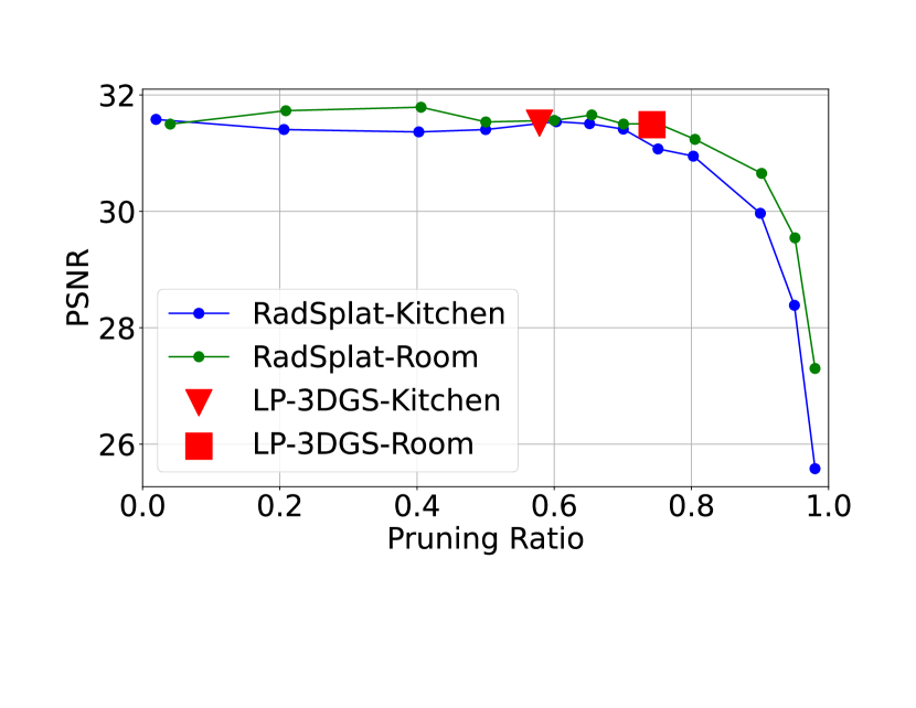
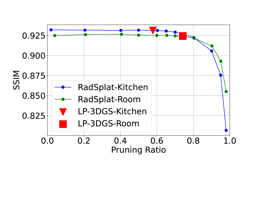
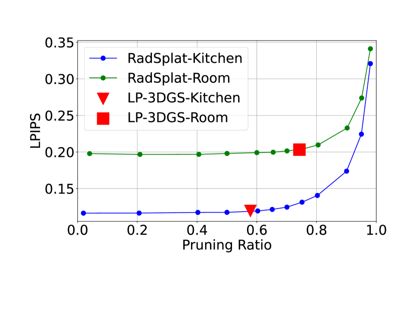
Figure 1: The performance changes with the pruning ratio of RadSplat on the MipNeRF360 dataset Kitchen and Room scenes are shown in blue and green lines, respectively. Red triangles and squares represent the results of LP-3DGS on the importance score of RadSplat. LP-3DGS is able to find the optimal pruning ratio in one training session instead of requiring dozens of attempts to find the best hyperparameter.

In this paper, we propose a learning-to-prune 3DGS (LP-3DGS) methodology where a trainable mask is applied to the importance score. Note that, it is compatible with different types of importance scores defined in prior works. Instead of a preset threshold to determine the 3DGS model pruning ratio, as shown by the red triangle symbol in the Figure 1, our method aims to integrate with existing 3DGS model training process to learn the optimal pruning ratio for minimizing the model size while maintaining the rendering quality. Since the traditional hard threshold based binary masking function is not differentiable, a recent prior work, Compact3D (Lee et al. (2023)), leverages the popular straight through estimator (STE) (Bengio et al. (2013)) to bypass the mask gradient for adaption to the backpropagation process. Such method inevitably leads to non-optimal learned pruning ratio. In contrast, in our work, we propose to redesign the masking function leveraging the Gumbel-Sigmoid activation function to make the whole masking function differentiable and integrate with the existing training process of 3DGS. As a result, our LP-3DGS could minimize the number of Gaussian points automatically for each scene with only one-time training.

In summary, the technical contributions of our work are:

• To address the effortful 3DGS optimal pruning ratio tuning, we propose a learning-to-prune 3DGS (LP-3DGS) methodology that leverages the differentiable Gumbel-Sigmoid activation function to embed a trainable mask with different types of existing importance scores designed for pruning redundant Gaussian points. As a result, instead of fixed model size, LP-3DGS could learn an optimal Gaussian point size for individual scene with only one-time training.

• We conducted comprehensive experiments on state-of-the-art (SoTA) 3D scene datasets, including MipNeRF360 (Barron et al. (2022)), NeRF-Synthetic (Mildenhall et al. (2021)), and Tanks & Temples (Knapitsch et al. (2017)). We compared our method with SoTA pruning methods such as RadSplat (Niemeyer et al. (2024)), Mini-Splatting (Fang and Wang (2024)), and Compact3D (Lee et al. (2023)). The experimental results show that our method can enable the model to learn the optimal pruning ratio and that our trainable mask method performs better than the STE mask.

2 Related Work

Neural radiance fields (NeRFs)

NeRFs (Mildenhall et al. (2021)) targets to represent the scene in multilayer perceptrons (MLPs) based on multi-view image inputs, enabling high-quality novel view synthesis. Due to its advancement, numerous follow-up works improved it in either rendering quality (Barron et al. (2021, 2022)) or efficiency(Müller et al. (2022); Chen et al. (2022); Fridovich-Keil et al. (2022)).

Although NeRF models demonstrate impressive rendering capabilities across numerous benchmarks, and considerable efforts have been made to enhance training and inference efficiency, they typically still face challenges in achieving fast training and real-time rendering.

Radiance Field Based On Points.

In addition to implicit representations, several works have focused on volumetric point-based methods for 3D presentation (Gross and Pfister (2011)). Inspired by neural network concepts, (Aliev et al. (2020)) introduced a neural point-based approach to streamline the construction process. Point-NeRF (Ding et al. (2024)) further applied points for volumetric representation, enhancing the effectiveness of point-based methods in radiance field modeling.

Gaussian Splatting

3D Gaussian Splatting (3DGS) (Kerbl et al. (2023)) represents a significant advancement in novel view synthesis, utilizing 3D Gaussians as primitives to explicitly represent scenes. This approach achieves state-of-the-art rendering quality and speed while maintaining relatively short training time. A series of methods have been introduced to improve the rendering quality through using regularization for better optimization, including depth map (Chung et al. (2023); Li et al. (2024a)), surface alignment (Guédon and Lepetit (2023); Li et al. (2024b)) and rendered image frequency (Zhang et al. (2024)). However, the extensive number of Gaussians required for scene representation often results in a model that is too large for efficient storage. Recent research has focused on compression methods to enhance the efficiency of this representation. Notably, several studies (Fan et al. (2023); Fang and Wang (2024); Niemeyer et al. (2024)) have proposed using predefined scores as pruning criteria to keep Gaussians that significantly contribute to rendering quality. Compact3D (Lee et al. (2023)) introduces a method that applies a trainable mask on scale and opacity to each Gaussian and utilizes a straight-through estimator (Bengio et al. (2013)) for gradient updates. LightGaussian (Fan et al. (2023)) employs knowledge distillation to reduce the dimension of spherical harmonics. Additionally, (Fan et al. (2023); Lee et al. (2023)) also explored quantization techniques to further compress model storage. The previously proposed pruning methods primarily rely on predefined scores to determine the importance of each Gaussian. These approaches present two main challenges: first, whether the criteria accurately reflect the importance of the Gaussians, and second, the need for a manually selected pruning threshold to decide the level of pruning. In this work, we address these issues by introducing a trainable mask activated by a Gumbel-sigmoid function, applied to the scores derived from prior methods or directly to the scale and opacity of each Gaussian for more flexibility. Our approach automatically identifies an optimal balance between the pruning ratio and rendering quality, eliminating the need to test on various pruning ratios.

3 Methodology

The conventional pruning methods leveraging predefined importance score require pruning ratio as a manually tuned parameter to reduce the size of Gaussian points in 3DGS. To seeking for the optimal pruning ratio, these methods may need to perform multiple rounds of training for each individual scene, which is inefficient. Thus motivated, we propose a learning-to-prune 3DGS (LP-3DGS) algorithm which learns a binary mask to determine the optimal pruning ratio for each scene automatically. Importantly, the proposed LP-3DGS is compatible with different types of pruning importance score. In this section, we will: 1) introduce the preliminary of the original 3DGS and recap different importance metrics for pruning that are proposed by prior works, and 2) present the proposed learning-to-prune 3DGS algorithm.

3.1 3DGS Background

3DGS Parameters

3DGS is an explicit point-based 3D representation that uses Gaussian points to model the scene. Each point has the following attributes: position $\bf{p}\in\mathbb{R}^{3}$, opacity $\sigma\in[0,1]$, scale in 3D $\bf{s}\in\mathbb{R}^{3}$, rotation presented by 4D quaternions $\bf{q}\in\mathbb{R}^{4}$ and forth-degree spherical harmonics (SH) coefficients $\bf{k}\in\mathbb{R}^{48}$. In summary, one gaussian point has 59 parameters. The center point $X$ of a Gaussian model is denoted by $\bf{p}$ and covariance matrix $\Sigma$ is denoted by $\bf{s}$ and $\bf{q}$. The SH coefficients model the color as viewed from different directions. The parameters of the Gaussians are optimized through gradient backpropagation of the loss between the rendered images and the ground truth.

Rendering on 3DGS

In order to render an image, the first step is projecting the Gaussians to 2D camera plane by world to camera transform matrix $W$ and Jacobian $J$ of affine approximation of the projective transform. The covariance matrix of projected 2D Gaussian is

$$\Sigma^{{}^{\prime}}=JW\Sigma W^{T}J^{T}$$ (1)

The projected Gaussians would be rendered as splat (Botsch et al. (2005)), the color of one pixel could be rendered as

$$\bf{c}_{i}=\sum_{j=1}^{N}\cdot\bf{c}_{j}\cdot\alpha_{j}\cdot T_{j}\cdot\bf{G}^{2D}_{j}$$ (2)

Where $i$ is the pixel index, $j$ is the Gaussian index and $N$ is the number of the Gaussians in the ray. $c_{j}$ is the color of the Gaussian calculated by SH coefficients, $\alpha_{j}=(1-exp^{-\sigma_{j}\delta_{j}})$, $\sigma_{j}$ is the opacity of the point and $\delta_{j}$ is the interval between points. $T_{j}=\prod_{k=1}^{j-1}(1-\alpha_{k})$ is the transmittance from the start of rendering to this point. $\bf{G}^{2D}_{j}$ is the 2D Gaussian distribution.

Adaptive Density Control of 3DGS

At the start of training, the Gaussians are initialized using Structure-from-Motion (SfM) sparse points. To make the Gaussians fit the scene better, 3DGS applies an adaptive density control strategy to adjust the number of Gaussians. Periodically, 3DGS will grow Gaussians in areas that are not well reconstructed, a process called "densification." Simultaneously, Gaussians with low opacity will be pruned.

3.2 Importance Metrics for Pruning

A straightforward way to prune the Gaussians is by sorting them based on a defined importance score and then removing the less important ones. As a result, one of the main objective of prior 3DGS pruning works is to define the importance metric.

RadSplat (Niemeyer et al. (2024)) defines the importance score as the maximum contribution along all rays of the training images, written as

$$\bf{S}_{i}=\max_{I_{f}\in\mathcal{I}_{f},r\in I_{f}}\alpha_{i}^{r}\cdot T_{i}^{r}$$ (3)

Where $\alpha_{i}^{r}\cdot T_{i}^{r}$ is the contribution of Gaussian $G_{i}$ along ray $r$. RadSplat performs pruning by applying a binary mask according to the importance score, where the mask value for Gaussian $G_{i}$ is

$$m_{i}=m(\bf{S}_{i})=\mathds{1}(\bf{S}_{i}<t_{prune})$$ (4)

Where $t_{prune}\in[0,1]$ is the threshold of score magnitude for pruning, $\mathds{1}[\cdot]$ is the indicator function.

Another recent work, Mini-Splatting (Fang and Wang (2024)), uses the cumulative weight of the Gaussian as the importance score, which can be formulated as:

$$\bf{S}_{i}=\sum_{j=1}^{K}\omega_{ij}$$ (5)

Where K is the total number of rays intersected with Gaussian $G_{i}$, $\omega_{ij}$ is the color weight of Gaussian $G_{i}$ on the $j$-th ray.

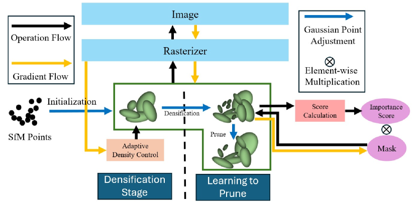
Figure 2: Overall learning process of the proposed LP-3DGS.

3.3 Learning-to-Prune 3DGS

The overall LP-3DGS learning process is shown in the Figure 2. In general, it mainly can be divided into two stages:1) densification stage, and 2) learning-to-prune stage. Following the original 3DGS, densification stage applies an adaptive density control strategy to gradually increase the number of Gaussians. As revealed by prior pruning works (Lee et al. (2023); Niemeyer et al. (2024)), 3DGS exists redundant Gaussians significantly. Subsequently, in the learning-to-prune stage, the proposed LP-3DGS learns a trainable mask upon prior defined importance metric to compress the number of Gaussians with an optimal pruning ratio automatically. Specifically, to learn a binary mask, we first initialize a real-value mask $m_{i}$ for each point $i$, and then adopt the Gumbel-sigmoid technique to binarize the mask value differentially.

Gumbel-Sigmoid based Trainable Mask

The binarization operation for real-value mask in pruning usually involves a hard threshold function, determining the binary mask should be 0 or 1. However, such hard threshold function is not differential during backpropagation. To solve this issue, popular straight through estimator (STE) method (Bengio et al. (2013)) is widely used which skips the gradient of the threshold function during backpropagation. Such process may lead to a gap between trainable real-value mask and binary mask. As shown in Figure 3(a), the trainable mask values exist certain ratios cross the whole range from 0 to 1 after Sigmoid function, which could be inaccurate when further converting to binary mask via a hard threshold function. To better optimize the trainable mask towards binary values, we propose to apply Gumbel-Sigmoid function to learn the binary mask.

The Gumbel distribution is used to model the extreme value distribution and generate samples from the categorical distribution (Gumbel (1954)). This property is then utilized to create the Gumbel-Softmax (Jang et al. (2016)), a differentiable categorical distribution sampling function. The sample of one category is given by:

$$y_{i}=\frac{\exp((\log(\pi_{i})+g_{i})/\tau)}{\sum_{j=1}^{k}\exp((\log(\pi_{j})+g_{j})/\tau)}$$ (6)

Where $\tau$ is the input adjustment parameter, $g_{i}$ is sample from Gumbel distribution. Inspired by the Gumbel-Softmax, we treat learning the binary mask of each point as a two-class category problem. Thus, we replace the Softmax function to Sigmoid function, referring to Gumbel-Sigmoid:

$$gs(m)=\frac{exp((\log(m)+g_{0})/\tau)}{exp((\log(m)+g_{0})/T)+exp(g_{1}/\tau)}=\frac{1}{1+exp(-(\log(m)+g_{0}-g_{1})/\tau)}$$ (7)

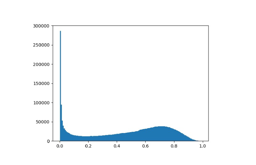
(a) Mask values after Sigmoid activation

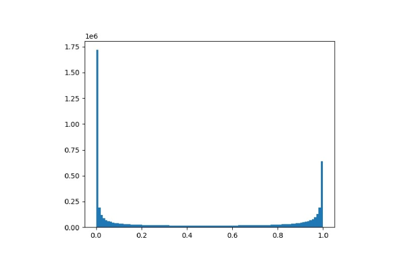
(b) Mask values after Gumbel-Sigmoid activation

Figure 3: Comparison between Sigmoid and Gumbel-Sigmoid. The Gumbel-Sigmoid function pushes the values closer to 0 or 1 and is a good approximation of a binarized mask.

By using such Gumbel-Sigmoid function, the output value is either close to 0 or 1, as shown in Figure 3, and thus can be utilized as an approximation of a binary masking function. More importantly, this function remains differentiable, thus can be integrated during backpropagation.

Moreover, to prune the selected Guassians practically according to the learned binary mask, we further apply the mask value on opacity, which can be mathematically formulated as

$$o_{im}=o_{i}*gs(m_{i}*S_{i})$$ (8)

where $S_{i}$ is the defined importance score of each Gaussian point. The closer the mask value is to 0, the less corresponding Gaussian point contributes to the rendering. In practice, after learning the trainable mask, a one-time pruning is applied to the corresponding Gaussian points with mask value of 0.

Sparsity regularization

In order to compress the model as much as possible, we apply a L1 regularization term (Lee et al. (2023)) to encourage the trainable mask to be sparse, which can be formulated as:

$$R_{mask}=\frac{1}{N}\sum_{i=1}^{N}\left|m_{i}\right|$$ (9)

Upon that, the final loss function is defined as:

$$L=(1-\lambda_{ssim})*L_{L1}+\lambda_{ssim}*L_{ssim}+\lambda_{m}*R_{mask}$$ (10)

$L_{L1}$ is the L1 loss between rendered image and ground truth. $L_{ssim}$ is the ssim loss. $\lambda_{ssim}$ and $\lambda_{m}$ are two coefficients.

Moreover, we find that the trainable mask can be effectively learned in just a few hundred iterations, compared to the thousands needed for the overall training process. In practice, the mask learning function is activated for only 500 iterations. Once the mask values are learned, we follow the 3DGS training setup to further fine-tune the pruned model, maintaining the same total number of training iterations. The detailed hyper parameters are described in the later experiment section.

4 Experiments

4.1 Experimental Settings

Dataset and Baseline

We test our method on two most popular real-world datasets: the MipNeRF360 dataset (Barron et al. (2022)), which contains 9 scenes, and the Train and Truck scenes from the Tanks & Temples dataset (Knapitsch et al. (2017)). We also test on the NeRF-Synthetic dataset (Mildenhall et al. (2021)), which includes 8 synthetic scenes. In this section, we only list the results on MipNeRF360 dataset, rest of them are listed in appendix A. In this paper, we use the SoTA RadSplat (Niemeyer et al. (2024)) and Mini-Splatting (Fang and Wang (2024)) as the baselines, which propose two different pruning importance scores. First, we test the performance of these two methods under different pruning ratios. Since neither method is open-sourced at the time of writing, we reproduced them based on the provided equations. For each pruning ratio, we calculate the corresponding threshold based on the magnitude of the importance scores and prune the Gaussians with scores below the threshold. Note that, each pruning ratio requires one round of training. We use peak signal-to-noise ratio (PSNR), structural similarity index measure (SSIM), and Learned Perceptual Image Patch Similarity (LPIPS) (Zhang et al. (2018)) as rendering evaluation metrics.

Implement Details

The machine running the experiments has an AMD 5955WX processor and two Nvidia A6000 GPUs. It should be noted that our method does not support multi-GPU training. We ran different experiments simultaneously on two GPUs. We train each scene under every setting for 30,000 iterations and train the mask during iterations 19,500 to 20,000, updating the importance score every 20 iterations. The $\tau$ in Equation 7 is 0.5 and the coefficient $\lambda_{m}$ of mask loss is 5e-4.

4.2 Experimental Results

Quantitative Results

The blue lines in Figure 4 show the results of sweeping pruning ratios using RadSplat and Mini-Splatting for the Kitchen, and Room scenes. Figures on other scenes of MipNeRF 360 are listed in Appendix A. The result of the learned LP-3DGS model size and rendering quality is indicated by red triangles.

PSNR $\uparrow$ SSIM $\uparrow$ LPIPS $\downarrow$

Kitchen

RadSplat

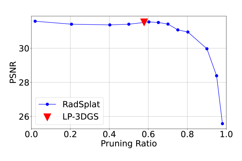
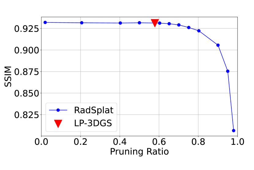
Mini-Splatting

Room

RadSplat

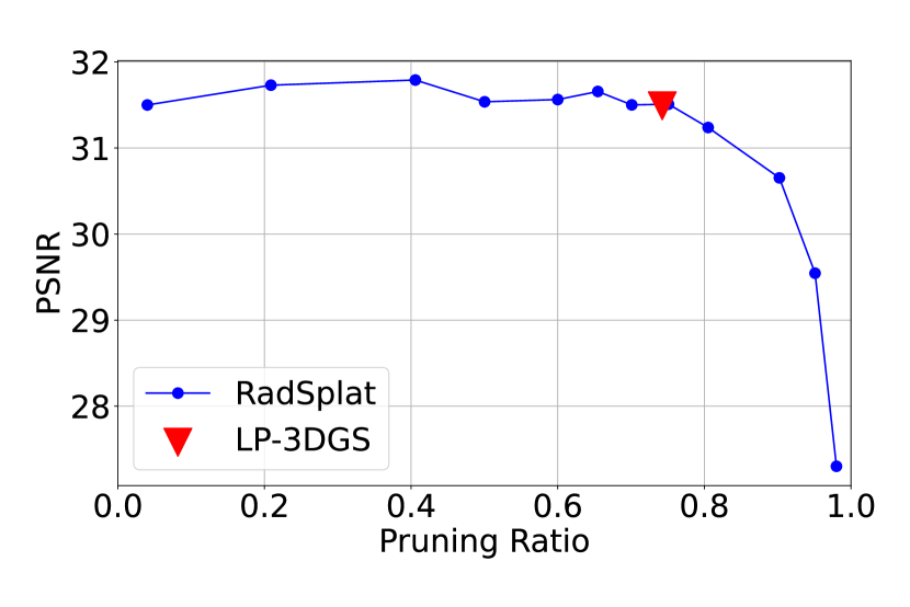
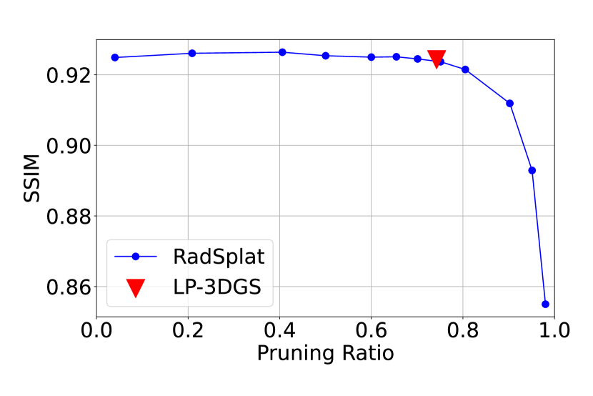
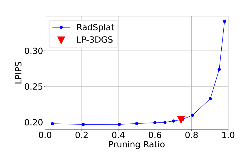
Mini-Splatting

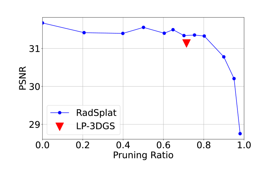
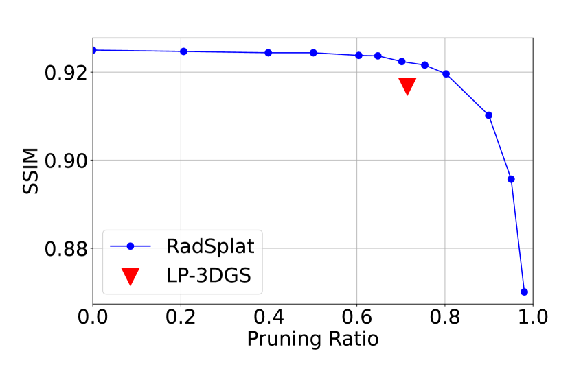
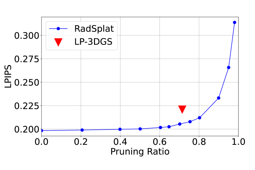
Figure 4: The performance changes with the pruning ratio in different scenes

The quantitative results fluctuate at lower pruning ratios but generally maintain around a certain value up to a specific point. After passing that point, the rendering quality decreases significantly. It’s worth noting that such decreasing point varies for different scenes. Instead of manually searching such optimal pruning ratio, it clearly shows our LP-3DGS method could learn the optimal model size embedding with the scene learning process, with only one-time training. The Table 1 lists the quantitative results of all scenes in MipNeRF360 dataset. It clearly shows that each scene converge into different model size leveraging our LP-3DGS method with maintaining almost the same rendering quality. The pruning ratio varies based on what importance score is used, but LP-3DGS could find the optimal pruning ratio on the corresponding score.

Table 1: The results comparison on the MipNeRF360 dataset shows that LP-3DGS has similar performance after pruning and achieves different pruning ratios for different scenes. This demonstrates LP-3DGS’s ability to adaptively find the optimal pruning ratio, maintaining performance while effectively compressing the model.

Scene Bicycle Bonsai Counter Kitchen Room Stump Garden Flowers Treehill AVG Baseline PSNR $\uparrow$ 25.087 32.262 29.079 31.581 31.500 26.655 27.254 21.348 22.561 27.48 LP-3DGS (RadSplat Score) 25.099 32.094 28.936 31.515 31.490 26.687 27.290 21.383 22.706 27.47 LP-3DGS (Mini-Splatting Score) 24.906 31.370 28.4098 30.785 31.132 26.679 27.095 21.150 22.522 27.12 Baseline SSIM $\uparrow$ 0.7464 0.9460 0.9138 0.9320 0.9249 0.7700 0.8557 0.5876 0.6358 0.8125 LP-3DGS (RadSplat Score) 0.7458 0.9441 0.9120 0.9311 0.9243 0.7714 0.8548 0.5865 0.6381 0.8120 LP-3DGS (Mini-Splatting Score) 0.7373 0.9358 0.9017 0.9249 0.9167 0.7677 0.8493 0.5756 0.6336 0.8047 Baseline LPIPS $\downarrow$ 0.2441 0.1799 0.1839 0.1164 0.1978 0.2423 0.1224 0.3601 0.3469 0.2215 LP-3DGS (RadSplat Score) 0.2516 0.1865 0.1896 0.1194 0.2032 0.2466 0.1270 0.3656 0.3527 0.2269 LP-3DGS (Mini-Splatting Score) 0.2642 0.2036 0.2068 0.1292 0.2208 0.2553 0.1353 0.3753 0.3618 0.2391 RadSplat Score pruning ratio 0.64 0.65 0.66 0.58 0.74 0.65 0.59 0.59 0.59 0.63 Mini-Splatting Score pruning ratio 0.57 0.67 0.64 0.56 0.71 0.61 0.60 0.54 0.54 0.60

Training Cost

Table 2 shows the training cost of LP-3DGS on MipNeRF360 dataset. In our setup, since after 20000th iteration, the model will be pruned based on the learned mask values. The number of Gaussian points will be significantly reduced, which makes the later stages of training take much less time than the non-pruned version. Even with the embedding of the mask learning function, the overall training cost is similar with that of the vanilla 3DGS. In most cases, the peak training memory usage is slightly larger because training the mask requires more GPU memory. However, after pruning, the 3DGS model size becomes much smaller, leading to a significant improvement in rendering speed, measured in terms of FPS.

Table 2: Training cost and on MipNeRF360 Dataset. Training time of LP-3DGS is similar with baseline but since the model is compressed, the FPS is larger.

Scene Bicycle Bonsai Counter Kitchen Room Stump Garden Flowers Treehill 3DGS Training time (Minute) 49 34 26 33 27 37 47 33 32 LP-3DGS (RadSplat Score) 43 27 28 34 30 35 46 34 33 LP-3DGS (Mini-Splatting Score) 44 27 28 35 29 34 46 34 33 3DGS Peak Memory (GB) 14.7 8.6 9.4 9.3 10.6 12.2 15.7 10.3 9.4 LP-3DGS (RadSplat Score) 16.1 8.5 11.3 12.3 11.8 12.1 15.8 10.1 10.3 LP-3DGS (Mini-Splatting Score) 15.5 8.4 12.7 13.0 13.0 12.1 15.2 9.7 9.7 3DGS FPS 132 417 421 315 380 164 129 200 205 LP-3DGS (RadSplat Score) 324 662 670 542 692 371 296 412 411 LP-3DGS (Mini-Splatting Score) 290 634 650 507 662 341 252 368 384

4.3 Ablation Study

A recent prior work Compact3D (Lee et al. (2023)) proposes to leverage STE to train a binary mask on opacity and scale of Gaussian parameter. To conduct a fair comparison between STE based mask and our LP-3DGS, we make two ablation studies, one is replacing the STE mask in Compact3D with our method, the other is applying STE mask on importance score of RadSpalt. The formula of STE mask is

$$M(m)=\mathrlap{\nabla}\hskip 0.5pt/\,(\mathds{1}[f(m)>\epsilon]-f(m))+f(m)$$ (11)

$\mathrlap{\nabla}\hskip 0.5pt/$ means stop gradients, $\mathds{1}[\cdot]$ is the indicator function and $f(\cdot)$ is sigmoid function, $\epsilon$ is masking threshold.

Comparison with Compact3D

We firstly apply Gumbel-sidmoid activated mask, instead of STE mask, on the opacity and scale of gaussians in the same way as proposed in Compact3D. The threshold $\epsilon$ in Equation 11 and mask loss coefficient follows the default settings in Compact3D. Table 3 shows the comparison between two methods.

Table 3: Results with/without trainable mask on Gaussian opacity and scale

Scene Bicycle Bonsai Counter Kitchen Room Stump Garden Flowers Treehill AVG PSNR Compact3D 24.846 32.19 29.066 30.867 31.489 26.408 27.026 21.187 22.479 27.284 LP-3DGS 25.087 32.2 29.033 31.213 31.678 26.658 27.223 21.32 22.569 27.442 SSIM Compact3D 0.7292 0.9462 0.9137 0.925 0.9251 0.7563 0.8446 0.5773 0.6305 0.8053 LP-3DGS 0.7438 0.9461 0.9141 0.9305 0.9263 0.7687 0.8547 0.5843 0.6358 0.8116 LPIPS Compact3D 0.266 0.1815 0.1866 0.124 0.2012 0.2615 0.1401 0.3722 0.3555 0.2320 LP-3DGS 0.2526 0.1833 0.1867 0.1201 0.2013 0.2472 0.1275 0.3668 0.3513 0.2263 #Gaussians Compact3D 2620663 666558 570126 1050079 566332 1902711 2412796 1685224 2089515 1507109 LP-3DGS 2510992 542235 506391 887161 479681 2014270 2836989 1747766 1804155 1481071

For most cases, our LP-3DGS learns a higher pruning ratio, except Stump, Garden and Flowers scene. In terms of rendering quality, our LP-3DGS outperforms compact3D using STE based mask with even smaller model size in most scenes.

STE Mask on Importance Score

We also apply STE mask on the pruning importance score to compare with our method. The Equation 8 would be rewriten as

$$o_{im}=o_{i}*M(m_{i}*is)$$ (12)

where $M$ is shown in Equation 11. The same as mentioned before, the parameters for STE mask are default values in Compact3D.

Table 4: Results using LP-3DGS and STE mask on importance score of RadSplat

Scene Bicycle Bonsai Counter Kitchen Room Stump Garden Flowers Treehill AVG PSNR LP-3DGS 25.099 32.094 28.936 31.515 31.490 26.687 27.290 21.383 22.706 27.470 STE mask 24.833 30.947 28.371 30.705 30.950 26.396 26.793 21.056 22.552 26.955 SSIM LP-3DGS 0.7458 0.9441 0.9120 0.9311 0.9243 0.7714 0.8548 0.5865 0.6381 0.8120 STE mask 0.7231 0.9268 0.8925 0.9162 0.9120 0.7514 0.8289 0.5624 0.6196 0.7922 LPIPS LP-3DGS 0.2441 0.1799 0.1839 0.1164 0.1978 0.2423 0.1224 0.3601 0.3469 0.2215 STE mask 0.2937 0.2194 0.2274 0.1480 0.2334 0.2899 0.1771 0.3988 0.3983 0.2651 Pruning Ratio LP-3DGS 0.64 0.65 0.66 0.58 0.74 0.65 0.59 0.59 0.59 0.63 STE mask 0.84 0.88 0.88 0.87 0.89 0.86 0.85 0.83 0.83 0.86

Table 4 shows that under the same settings, after applying the mask to the importance score, the STE mask compresses the mode too much and the performance drops a lot. Trainable mask keeps the gradient of the mask and the comressed model has a more reasonable size.

Table 5: Results using LP-3DGS and STE mask on importance score of Mini-Splatting

Scene Bicycle Bonsai Counter Kitchen Room Stump Garden Flowers Treehill AVG PSNR LP-3DGS 24.906 31.370 28.4098 30.785 31.132 26.679 27.095 21.150 22.522 27.12 STE mask 24.894 30.925 28.334 30.731 31.032 26.470 26.863 20.997 22.559 26.98 SSIM LP-3DGS 0.7373 0.9358 0.9017 0.9249 0.9167 0.7677 0.8493 0.5756 0.6336 0.8047 STE mask 0.7287 0.9292 0.8978 0.9232 0.9152 0.7562 0.8381 0.5629 0.6247 0.7973 LPIPS LP-3DGS 0.2642 0.2036 0.2068 0.1292 0.2208 0.2553 0.1353 0.3753 0.3618 0.2391 STE mask 0.2821 0.2154 0.2145 0.1330 0.2241 0.2797 0.1564 0.3939 0.3852 0.2538 Pruning Ratio LP-3DGS 0.57 0.67 0.64 0.56 0.71 0.61 0.60 0.54 0.54 0.60 STE mask 0.75 0.77 0.75 0.66 0.79 0.80 0.75 0.75 0.75 0.75

5 Discussion and Conclusion

Broader Impact and Limitation

LP-3DGS compresses the 3DGS model to an ideal size in a single run, saving storage and computational resources by eliminating the need for parameter sweeping to find the optimal pruning ratio. However, the limitation of this work is that the rendering quality after pruning varies depending on the definition of importance scores.

Conclusion

In this paper, we present a novel framework, LP-3DGS, which guide the 3DGS model learn the best model size. The framework applies a trainable mask on the importance score of the gaussian points. The mask only would be trained for a certain period and prune the model once. Our method compressed the model as much as possible without significantly sacrificing performance and is able to achieve the optimal compression rate for different test scenes. Compared with STE mask method, ours achieves better performance.

Appendix A Appendix / supplemental material

Code: https://github.com/dexgfsdfdsg/LP-3DGS.git

A.1 Experiment Results on MipNeRF360 Dataset

Ground Truth 3DGS RadSplat Mini-Splatting

Bicycle

Bonsai

Counter

Kitchen

Room

Stump

Garden

Flowers

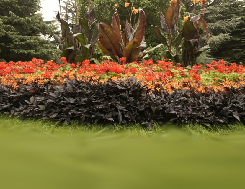
Treehill

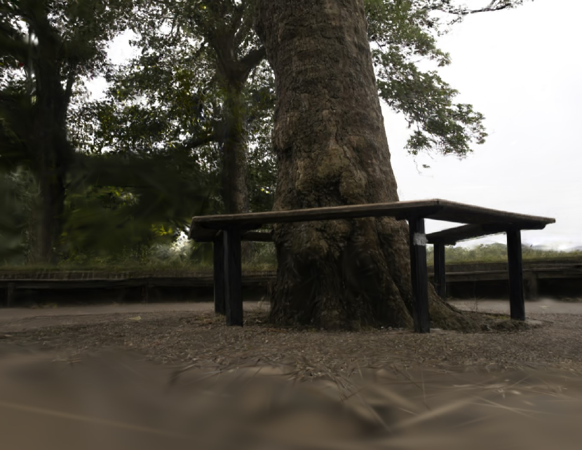
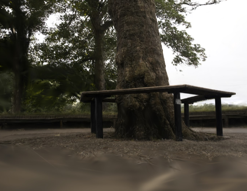
Figure 5: Rendered images on MipNeRF360 Dataset

PSNR $\uparrow$ SSIM $\uparrow$ LPIPS $\downarrow$

Bicycle

RadSplat

Mini-Splatting

Bonsai

RadSplat

Mini-Splatting

Counter

RadSplat

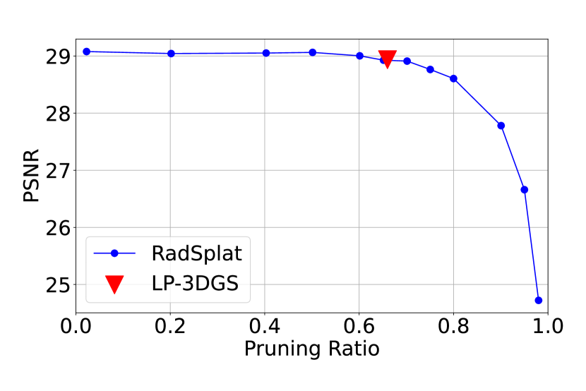
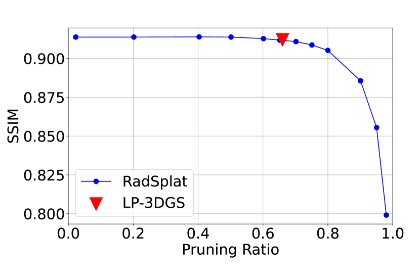
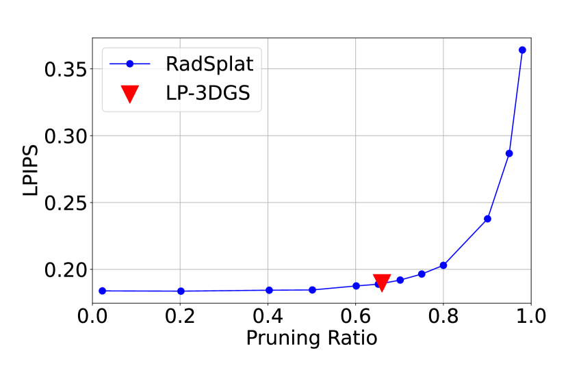
Mini-Splatting

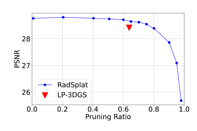
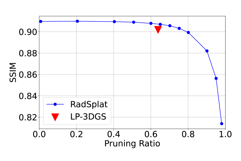
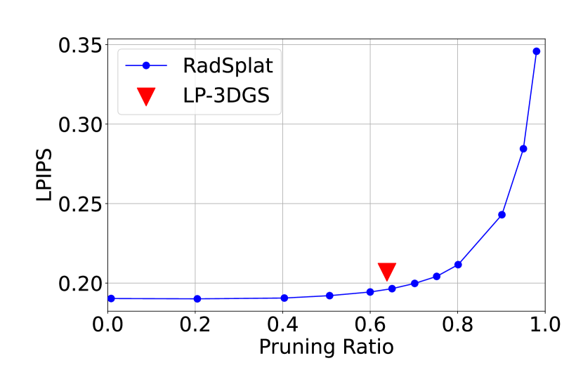
Stump

RadSplat

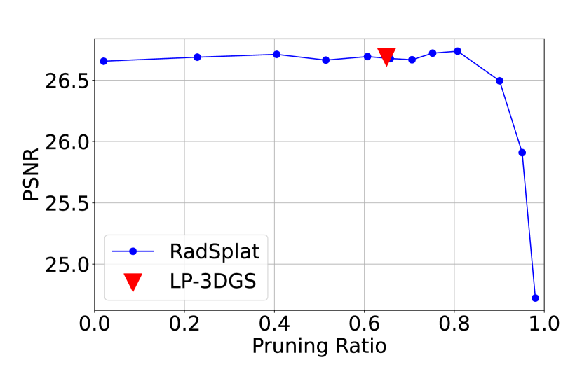
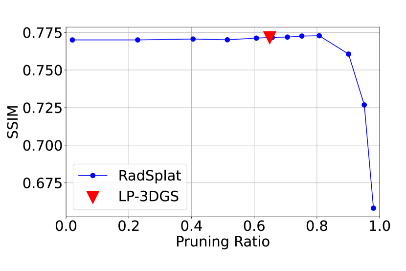
Mini-Splatting

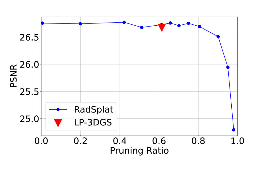
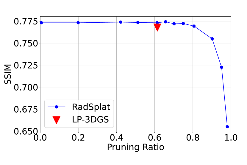
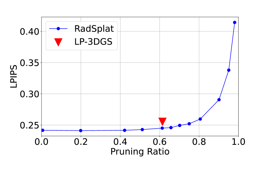
Flowers

RadSplat

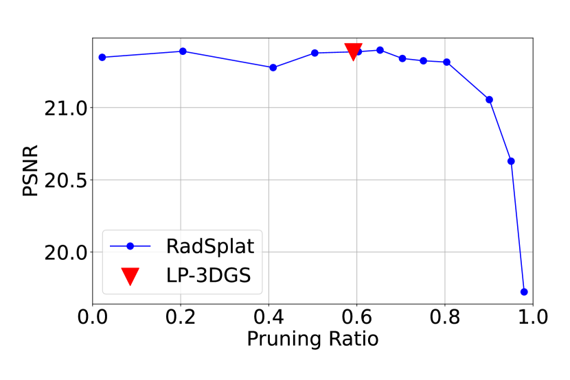
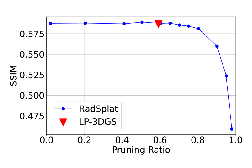
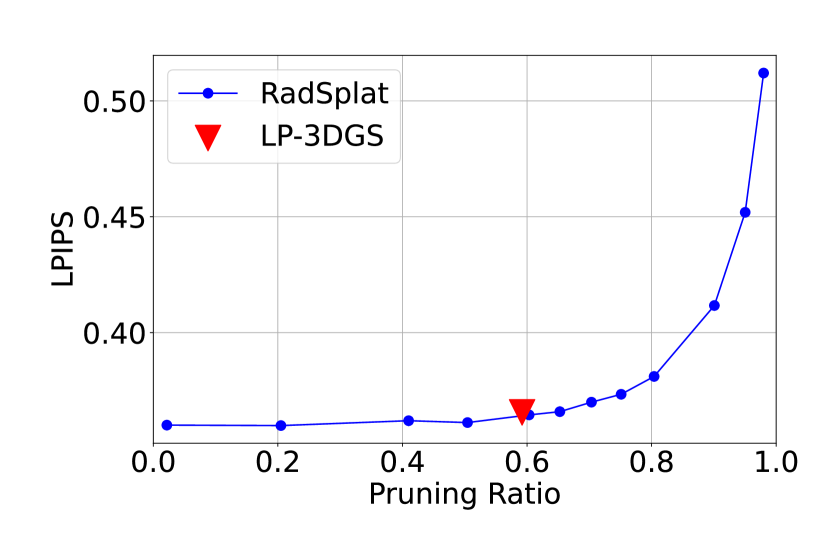
Mini-Splatting

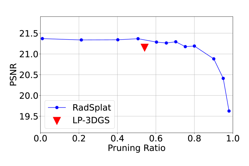
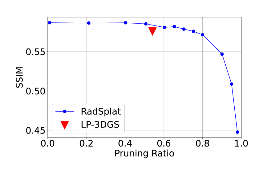
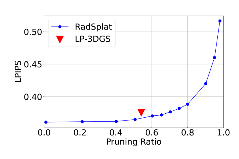
Treehill

RadSplat

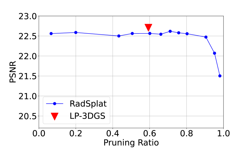
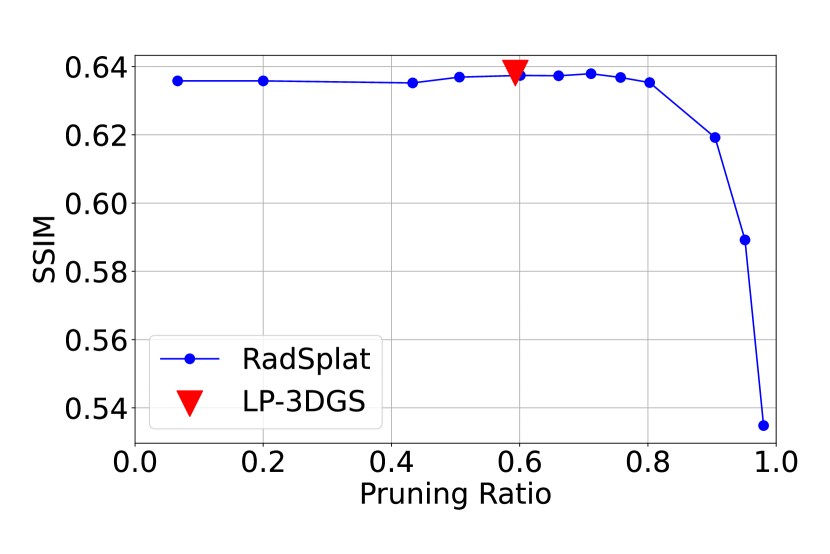
Mini-Splatting

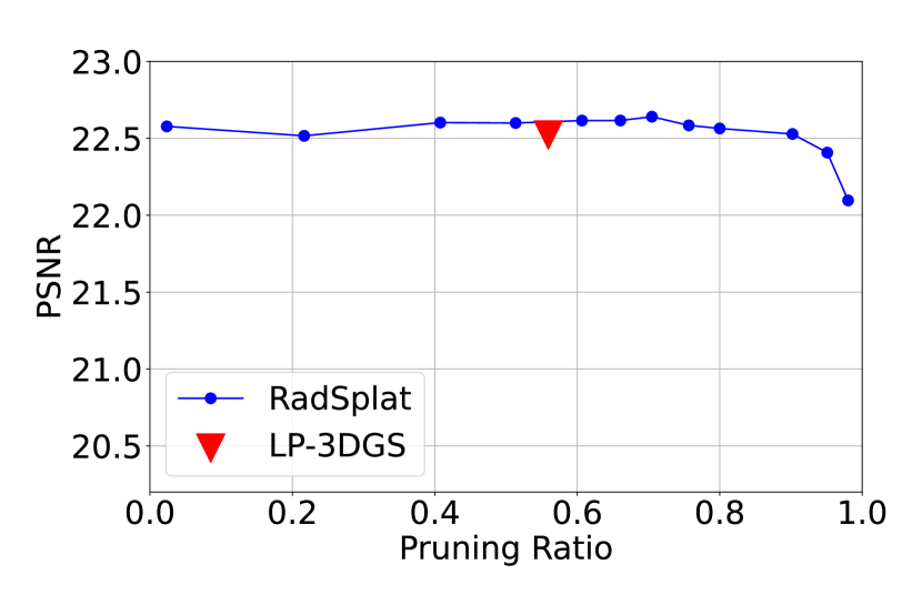
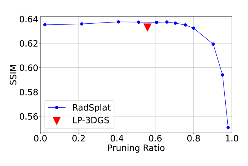
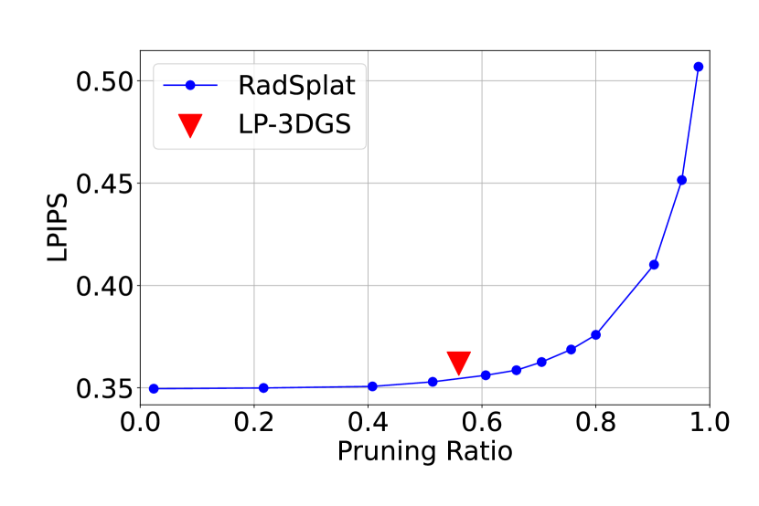
Figure 6: The performance changes with the pruning ratio in different scenes

A.2 Experiment Results on NeRF Synthetic Dataset

Table 6: The quantitative results on NeRF Synthetic Dataset

Scene Chair Drums Ficus Hotdog Lego Materials Mic Ship AVG Baseline PSNR $\uparrow$ 35.546 26.276 35.480 38.081 36.012 30.502 36.795 31.688 33.798 LP-3DGS (RadSplat Score) 35.496 26.221 35.442 37.976 35.990 30.374 36.589 31.584 33.709 LP-3DGS (Mini-Splatting Score) 35.419 26.102 35.354 37.728 35.769 29.883 36.337 31.375 33.496 Baseline SSIM $\uparrow$ 0.9877 0.9548 0.9870 0.9854 0.9825 0.9604 0.9926 0.9062 0.9696 LP-3DGS (RadSplat Score) 0.9878 0.9547 0.9867 0.9854 0.9825 0.9598 0.9924 0.9061 0.9694 LP-3DGS (Mini-Splatting Score) 0.9874 0.9358 0.9867 0.9846 0.9817 0.9566 0.9919 0.9034 0.966 Baseline LPIPS $\downarrow$ 0.01046 0.03657 0.01775 0.01977 0.0161 0.03671 0.00635 0.1058 0.03119 LP-3DGS (RadSplat Score) 0.01091 0.03723 0.01213 0.02079 0.01675 0.03817 0.00680 0.1083 0.03139 LP-3DGS (Mini-Splatting Score) 0.0111 0.03876 0.01217 0.02211 0.018 0.04323 0.00749 0.1151 0.0335 RadSplat Score pruning ratio 0.77 0.76 0.84 0.68 0.65 0.61 0.78 0.60 0.71 Mini-Splatting Score pruning ratio 0.63 0.65 0.65 0.58 0.58 0.80 0.60 0.50 0.62

A.3 Experiment Results on Truck & Train Scenes

Table 7: The quantitative results on Tanks & Temples Dataset

Scene Truck Train AVG Baseline PSNR $\uparrow$ 25.263 22.025 23.644 LP-3DGS (RadSplat Score) 25.376 21.822 23.599 LP-3DGS (Mini-Splatting Score) 25.152 21.675 23.414 Baseline SSIM $\uparrow$ 0.8778 0.8118 0.8448 LP-3DGS (RadSplat Score) 0.8768 0.8072 0.8420 LP-3DGS (Mini-Splatting Score) 0.8724 0.7963 0.8344 Baseline LPIPS $\downarrow$ 0.1482 0.2083 0.1783 LP-3DGS (RadSplat Score) 0.1541 0.2217 0.1879 LP-3DGS (Mini-Splatting Score) 0.162 0.2343 0.1982 RadSplat Score pruning ratio 0.72 0.63 0.68 Mini-Splatting Score pruning ratio 0.65 0.57 0.61

References

- Mildenhall et al. [2021] Ben Mildenhall, Pratul P Srinivasan, Matthew Tancik, Jonathan T Barron, Ravi Ramamoorthi, and Ren Ng. Nerf: Representing scenes as neural radiance fields for view synthesis. Communications of the ACM, 65(1):99–106, 2021.
- Kerbl et al. [2023] Bernhard Kerbl, Georgios Kopanas, Thomas Leimkühler, and George Drettakis. 3d gaussian splatting for real-time radiance field rendering. ACM Transactions on Graphics, 42(4):1–14, 2023.
- Fan et al. [2023] Zhiwen Fan, Kevin Wang, Kairun Wen, Zehao Zhu, Dejia Xu, and Zhangyang Wang. Lightgaussian: Unbounded 3d gaussian compression with 15x reduction and 200+ fps. arXiv preprint arXiv:2311.17245, 2023.
- Niemeyer et al. [2024] Michael Niemeyer, Fabian Manhardt, Marie-Julie Rakotosaona, Michael Oechsle, Daniel Duckworth, Rama Gosula, Keisuke Tateno, John Bates, Dominik Kaeser, and Federico Tombari. Radsplat: Radiance field-informed gaussian splatting for robust real-time rendering with 900+ fps. arXiv preprint arXiv:2403.13806, 2024.
- Fang and Wang [2024] Guangchi Fang and Bing Wang. Mini-splatting: Representing scenes with a constrained number of gaussians. arXiv preprint arXiv:2403.14166, 2024.
- Barron et al. [2022] Jonathan T Barron, Ben Mildenhall, Dor Verbin, Pratul P Srinivasan, and Peter Hedman. Mip-nerf 360: Unbounded anti-aliased neural radiance fields. In Proceedings of the IEEE/CVF Conference on Computer Vision and Pattern Recognition, pages 5470–5479, 2022.
- Lee et al. [2023] Joo Chan Lee, Daniel Rho, Xiangyu Sun, Jong Hwan Ko, and Eunbyung Park. Compact 3d gaussian representation for radiance field. arXiv preprint arXiv:2311.13681, 2023.
- Bengio et al. [2013] Yoshua Bengio, Nicholas Léonard, and Aaron Courville. Estimating or propagating gradients through stochastic neurons for conditional computation. arXiv preprint arXiv:1308.3432, 2013.
- Knapitsch et al. [2017] Arno Knapitsch, Jaesik Park, Qian-Yi Zhou, and Vladlen Koltun. Tanks and temples: Benchmarking large-scale scene reconstruction. ACM Transactions on Graphics (ToG), 36(4):1–13, 2017.
- Barron et al. [2021] Jonathan T Barron, Ben Mildenhall, Matthew Tancik, Peter Hedman, Ricardo Martin-Brualla, and Pratul P Srinivasan. Mip-nerf: A multiscale representation for anti-aliasing neural radiance fields. In Proceedings of the IEEE/CVF International Conference on Computer Vision, pages 5855–5864, 2021.
- Müller et al. [2022] Thomas Müller, Alex Evans, Christoph Schied, and Alexander Keller. Instant neural graphics primitives with a multiresolution hash encoding. ACM transactions on graphics (TOG), 41(4):1–15, 2022.
- Chen et al. [2022] Anpei Chen, Zexiang Xu, Andreas Geiger, Jingyi Yu, and Hao Su. Tensorf: Tensorial radiance fields. In European Conference on Computer Vision, pages 333–350. Springer, 2022.
- Fridovich-Keil et al. [2022] Sara Fridovich-Keil, Alex Yu, Matthew Tancik, Qinhong Chen, Benjamin Recht, and Angjoo Kanazawa. Plenoxels: Radiance fields without neural networks. In Proceedings of the IEEE/CVF Conference on Computer Vision and Pattern Recognition, pages 5501–5510, 2022.
- Gross and Pfister [2011] Markus Gross and Hanspeter Pfister. Point-based graphics. Elsevier, 2011.
- Aliev et al. [2020] Kara-Ali Aliev, Artem Sevastopolsky, Maria Kolos, Dmitry Ulyanov, and Victor Lempitsky. Neural point-based graphics. In Computer Vision–ECCV 2020: 16th European Conference, Glasgow, UK, August 23–28, 2020, Proceedings, Part XXII 16, pages 696–712. Springer, 2020.
- Ding et al. [2024] Yuhan Ding, Fukun Yin, Jiayuan Fan, Hui Li, Xin Chen, Wen Liu, Chongshan Lu, Gang Yu, and Tao Chen. Point diffusion implicit function for large-scale scene neural representation. Advances in Neural Information Processing Systems, 36, 2024.
- Chung et al. [2023] Jaeyoung Chung, Jeongtaek Oh, and Kyoung Mu Lee. Depth-regularized optimization for 3d gaussian splatting in few-shot images. arXiv preprint arXiv:2311.13398, 2023.
- Li et al. [2024a] Jiahe Li, Jiawei Zhang, Xiao Bai, Jin Zheng, Xin Ning, Jun Zhou, and Lin Gu. Dngaussian: Optimizing sparse-view 3d gaussian radiance fields with global-local depth normalization. arXiv preprint arXiv:2403.06912, 2024a.
- Guédon and Lepetit [2023] Antoine Guédon and Vincent Lepetit. Sugar: Surface-aligned gaussian splatting for efficient 3d mesh reconstruction and high-quality mesh rendering. arXiv preprint arXiv:2311.12775, 2023.
- Li et al. [2024b] Yanyan Li, Chenyu Lyu, Yan Di, Guangyao Zhai, Gim Hee Lee, and Federico Tombari. Geogaussian: Geometry-aware gaussian splatting for scene rendering. arXiv preprint arXiv:2403.11324, 2024b.
- Zhang et al. [2024] Jiahui Zhang, Fangneng Zhan, Muyu Xu, Shijian Lu, and Eric Xing. Fregs: 3d gaussian splatting with progressive frequency regularization. arXiv preprint arXiv:2403.06908, 2024.
- Botsch et al. [2005] Mario Botsch, Alexander Hornung, Matthias Zwicker, and Leif Kobbelt. High-quality surface splatting on today’s gpus. In Proceedings Eurographics/IEEE VGTC Symposium Point-Based Graphics, 2005., pages 17–141. IEEE, 2005.
- Gumbel [1954] Emil Julius Gumbel. Statistical theory of extreme values and some practical applications: a series of lectures, volume 33. US Government Printing Office, 1954.
- Jang et al. [2016] Eric Jang, Shixiang Gu, and Ben Poole. Categorical reparameterization with gumbel-softmax. arXiv preprint arXiv:1611.01144, 2016.
- Zhang et al. [2018] Richard Zhang, Phillip Isola, Alexei A Efros, Eli Shechtman, and Oliver Wang. The unreasonable effectiveness of deep features as a perceptual metric. In Proceedings of the IEEE conference on computer vision and pattern recognition, pages 586–595, 2018.