Benchmarking the Exponential Ansatz for the Holstein model
Abstract
Polarons are quasiparticles formed as a result of lattice distortions induced by charge carriers. The single-electron Holstein model captures the fundamentals of single polaron physics. We examine the power of the exponential ansatz for the polaron ground-state wavefunction in its coupled cluster, canonical transformation, and (canonically transformed) perturbative variants across the parameter space of the Holstein model. Our benchmark serves to guide future developments of polaron wavefunctions beyond the single-electron Holstein model.
I Introduction
Electron-phonon interactions play an essential role in many solid-state materials [1]. Polarons are quasiparticles formed due to a strong electron-phonon interaction, which results in the trapping of electrons by localized lattice distortions [2]. Polaron phenomenology has been extensively studied through lattice models and semi-empirical Hamiltonians. Out of these, the simplest is probably the Holstein model [3], whose phase diagram captures both the phenomenon of polaron formation and the crossover between small and large polaron regimes. Despite the model’s simplicity, analytical techniques are only applicable under restricted conditions [4]. Thus most results have been obtained by applying numerical methods, including exact diagonalization (ED) [5, 6], density matrix renormalization group (DMRG) [7], variational wavefunctions [8, 9, 10, 11, 12], perturbation theories [13, 14, 15], and canonical transformation formalisms [16, 17, 18].
The current work studies and benchmarks the exponential electron-phonon ansatz for the single-electron Holstein model. We consider two specific kinds of exponential ansatz. The first, coupled cluster theory, is widely recognized as a highly accurate method in computational chemistry [19, 20, 21, 22, 23, 24]. Here we use the electron-phonon coupled cluster formalism introduced by some of us in Ref. [25]. The second is the well-known variational Lang-Firsov ansatz and its recently introduced perturbation theory, as discussed in Ref. [26] also by some authors of this work. The variational Lang-Firsov ansatz [14] can be viewed as a unitary coupled cluster theory, and thus fits within the family of exponential ansatz wavefunctions. We study the numerical performance of these methods across different parameters of the model, benchmarking against converged exact results from density matrix renormalization group simulations [7, 27, 28]. In additional to the energy, we examine multiple observables that characterize polaron formation and the transition between large and small polarons.
II Theory
II.1 Holstein Model
The single-electron Holstein model defines a minimal spinless one-electron lattice model containing interactions between a single electron band and a set of local phonons. The Hamiltonian for a -site one-dimensional Holstein model is
| (1) | ||||
where () creates (annihilates) an electron on site , and () creates (annihilates) a phonon of frequency on site , is the electron number operator on site , and periodic boundary conditions are assumed. The electron-phonon coupling parameter is denoted as , and we set the hopping parameter to be (thus all energy values will implicitly be in units of ).
The physics of the Holstein model can be understood in different limiting cases. Defining the adiabaticity parameter as , corresponds to a slow response of the lattice distortion to electron hopping. In this scenario, the Born-Oppenheimer approximation is valid and the electronic motion is consequently modified by quasi-static lattice deformations (i.e. an adiabatic potential surface). Alternatively, when (the anti-adiabatic limit), the lattice deformation adapts instantaneously to the electron’s position. Then, only the vibrational ground state is involved in low-energy electron hopping processes.
Another axis along which to understand the physics is with respect to the electron-phonon coupling itself. In the weak coupling regime, defined by and , the system resembles a quasi-free electron dragging a phonon cloud: this is known as a large polaron. In contrast, in the strong coupling regime, the electronic position is closely correlated with the lattice distortion it generates: this is known as a small polaron, which is referred to as self-trapped. Although some early analytical perturbation theory suggested a sharp transition between the two [29, 30], it has been established from rigorous analysis that there is a smooth crossover between the small and large polaron limits [4]. The accurate description of the self-trapping crossover represents a challenge for most computational methods [15].
The exact ground-state of the Holstein model can be expressed as
| (2) |
where is a configuration of the electron-phonon system,
| (3) |
with an electronic state on site , which can be either empty or singly occupied, and is the phonon occupation state on site , which is a number between and where is the maximum local phonon number. The number of configurations in the above is , and should be taken to infinity for converged results. The rapid growth in the number of configurations with both and limits the usefulness of exact diagonalization (ED) and motivates the study of approximate ansatzes. We focus on two variants of the exponential ansatz for the ground-state: the coupled cluster method and the Lang-Firsov transformation. For benchmarking purposes, we employ the density matrix renormalization group (DMRG), which provides highly accurate results for finite , but where must be extrapolated: this is described in Appendix A.
II.2 Reference states
The coupled cluster and Lang-Firsov methods require a starting reference state. We will assume the reference state to be a product state of a single-particle electronic orbital and a site-dependent coherent state,
| (4) |
where and are the physical vacua for electrons and phonons respectively.
In the simplest case, which we refer to as the mean-field (MF) reference state, and are chosen to minimize the energy , with and . represents the equilibrium shift of the phonon mode at site induced by the electron density. The optimal either satisfies translational invariance (delocalized) or it breaks translational invariance (localized). These two solutions, , respectively, are favoured in different regimes of the Holstein model parameter space, and can be viewed as a mean-field description of the self-trapping crossover. However, it is known that the mean-field description is not accurate in this region, and an important test of the more sophisticated exponential ansatzes we explore on top of these mean-field reference states is to see how well they improve the description of the crossover.
An alternative is to reoptimize and improve and in the presence of the exponential ansatz parameters. We discuss this option below.
II.3 Coupled Cluster Models for Electron-phonon Systems
| model | scaling | |||
|---|---|---|---|---|
| CCS-1-S1 | ||||
| CCS-2-S2 | ||||
| LF-HF | 0 | 0 |
The coupled cluster method for electron-phonon systems is formulated based on the exponential wavefunction ansatz [31],
| (5) |
where the excitation operator consists of an electronic part, a phononic part, and a coupling:
| (6) | ||||
where , are occupied and virtual electronic orbital indices, and are used for site indices for the boson operators. The truncation of the excitation operator determines the accuracy and cost scaling of the method. Given the one-electron nature of the Holstein model, there is only a single occupied electronic orbital (i.e. a single index value for , with the form of the orbital specified by in Eq 4), and the electronic excitations are captured exactly using singles excitations of the form , thus we truncate the electronic excitation to this level, referred to as singles. The order of the phonon and coupling excitations is then denoted by X-SY, where X, Y are numbers that show the excitation order. For example, CCS-1-S1 indicates single electronic excitations, single phonon excitations, and single coupled excitations, corresponding to the excitation operator . The formulae and the scaling of the CC models considered in this work are shown in Table 1. (It is helpful to recognize that the models we consider are invariant to shifts of the boson operators e.g. and , in the sense that any such shift can be absorbed into a redefinition of the coupled cluster amplitudes).
The amplitudes are obtained by solving the projected Schrödinger equation:
| (7) |
and the energy is obtained from
| (8) |
where is the coupled cluster effective Hamiltonian. The same equations have also been used in coupled cluster theories for cavity polaritons that have been independently developed in Refs. [32, 33, 34]. In this study, all the coupled cluster equations were formulated using the Wick package and solved using the Newton-Krylov method, which approximates the inverse Jacobian matrix using the Krylov subspace method [35, 36]. Note that as all matrix elements are evaluated using Wick’s theorem, there is no need to truncate the phonon number.
Because the energy is defined from an asymmetric expectation value, the coupled cluster energy is not necessarily variational. In addition, it does not satisfy a Hellman-Feynman theorem, thus in order to obtain observables other than the energy, we instead define a coupled cluster Lagrangian [24],
| (9) | ||||
where are the Lagrange multipliers corresponding to the amplitude equations; leads to the coupled cluster working equations in Eq. 7; leads to the equations for the Lagrangian multipliers. The expectation value of the observable is then,
| (10) |
The mean-field optimization of the reference in Eq. 4 already allows for a non-trivial mean-field state (e.g. a localized mean-field state), and we start the coupled cluster equations from both the localized and delocalized mean-field solutions. We also consider a further orbital optimization to make the coupled clus1ter Lagrangian stationary, corresponding to the ansatz
| (11) |
where are the parameters in Eq. 4, relaxed in the presence of the coupled cluster correlations, and the amplitude are also updated with the orbital parameters. We refer to this mean-field reference as . (In practice, we relax and update parametrically via as we did in the self-consistent optimization of Eq. 4; we find in the Lang-Firsov simulations below that there is little difference between independent optimization of and using this parametric choice).
II.4 Variational Lang-Firsov Approach and Perturbation Theory
The Lang-Firsov (LF) transformation is a unitary exponential ansatz to obtain the ground state. In this study, our focus is solely on the diagonal formulation of the Lang-Firsov parameters [26],
| (12) |
| (13) |
and the energy is
| (14) |
where is the Lang-Firsov Hamiltonian. In the coupled cluster classification this ansatz is a unitary coupled cluster model containing only a type of first-order operator, i.e. a variant of unitary CC0-0-S1, although we refer to it as LF below.
Just as with the coupled cluster ansatz, the LF energy can be computed from different choices of , and we consider both the delocalized and localized mean-field solutions of Eq. 4. In addition, we also reoptimize the reference state in the presence of the electron-phonon correlations. This corresponds to defining
| (15) |
and using the analytic gradients obtained in Ref. [26], we minimize with respect to all the parameters. In Ref. [26], this fully optimized Lang-Firsov state is referred to as the Lang-Firsov Hartree-Fock (LF-HF) energy.
To incorporate additional electron-phonon correlation, we can carry out perturbation theory.
Similar to the conventional Møller-Plesset (MP) theory utilized in electronic structure theories, we define the zeroth-order Hamiltonian as
| (16) |
where is the effective electronic Hamiltonian , where is the phonon part of the state defined in Eq. 4. is an eigenstate of and the corresponding energy is .
The fluctuation potential is then
| (17) |
The corresponding first-order energy correction is
| (18) |
| (19) |
which is exactly the LF energy. We then consider the second-order energy correction,
| (20) |
where , as described in Eq. 6. We evaluate it in a space of electron-phonon configurations following Ref. [26], which requires a truncation of the phonon number. Here, we choose to truncate at 10 phonons per site.
III Results and Discussions
We apply the methods described in Section II to the one-dimensional Holstein model within the parameter space of and in units of . We use converged DMRG results as the reference, and the convergence of this data is discussed in Appendix A.
III.1 Role of the reference
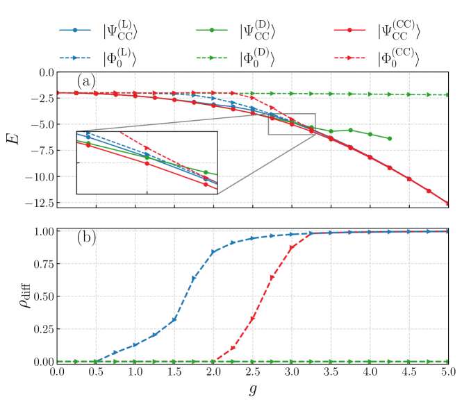
We first discuss the role of the reference state for the coupled cluster method in describing the physics of the Holstein model. We consider the following choices of reference state for the coupled cluster method: (i) the lowest energy optimized mean-field state allowing for (potential) breaking of translational invariance. This reference state is denoted and the corresponding exponential ansatz as ; (ii) the delocalized reference state with and , denote as with the corresponding ; and (iii) the reference state that minimizes the coupled cluster energy, denoted as with the corresponding .
We present results from the 64-site Holstein model with . Fig. 1 (a) shows the energy of the reference states (dashed lines) and the corresponding CCS-2-S2 energies (solid lines); Fig. 1 (b) plots the density difference of the reference states as a descriptor of the localization of the reference states. Note that for any coupling constant , the exact solution predicts a uniform electron density in the ground state. All reference states coincide for small values of . However, as increases beyond a critical , and start to transform into localized states with lower energies than the delocalized reference state . It is important to note that although can be obtained for all , we are unable to converge the coupled cluster amplitude equations in the strong coupling regime and thus cannot obtain . The presence of electron-phonon correlation in the optimization of the reference state in shifts the critical towards a larger value. The density differences in Fig. 1 (b) also reflect a smaller amount of symmetry breaking in the compared to . Interestingly, near the transition () the lowest energy mean-field reference does not result in the lowest energy coupled cluster energy. As shown in the zoomed-in plot, while corresponds to the lowest mean-field energy, the energies of both and are lower.
The above illustrates the importance of choosing an appropriate reference when using an exponential ansatz. In the sections below, we always use the optimized reference state (iii) for the coupled cluster methods, and perform the full reoptimization of in the LF-HF and LF-MP2 calculations.
III.2 Energy across parameter space
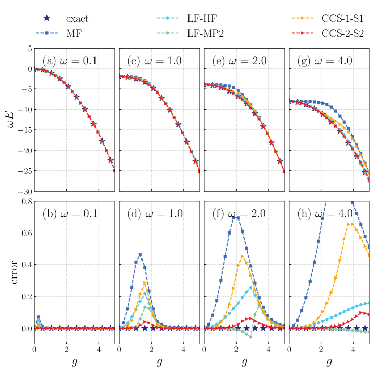
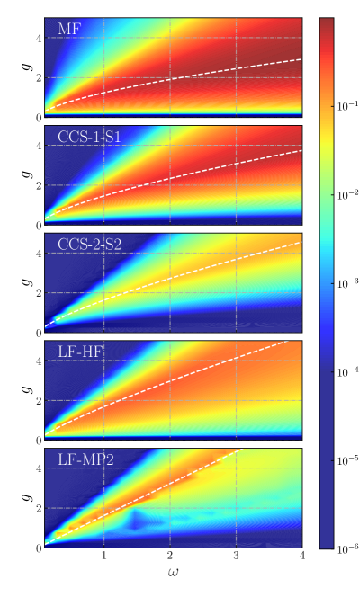
We now examine the energy errors across the Holstein parameters space for Lang-Firsov and coupled cluster ansatzes. Fig. 2 plots the ground state energy error in the 2D parameter space of and for the 64-site Holstein model, while slices through this space are shown in Fig. 3 for and . All methods presented are accurate for and in the strong coupling regimes, and display most variation in accuracy in the intermediate coupling regime. The dashed lines in Fig. 3 represent the coupling strength at the given frequency where the method exhibits its largest error. From this we can conclude that the accuracy roughly follows MFCCS-1-S1LF-HFLF-MP2CCS-2-S2. Similar conclusions can be drawn from Fig. 3. These slices additionally show that the mean-field error is largest in the anti-adiabatic () regime. Despite the similarity of the LF-HF and CCS-1-S1 parametrizations, LF-HF outperforms CCS-1-S1 in this regime: the unitary variational optimization of LF-HF clearly contributes to the improved behaviour in this limit. We see also that LF-MP2 has a discontinuity in the energy at intermediate decoupling, which does not appear in the coupled cluster results.
III.3 Electronic Kinetic Energy
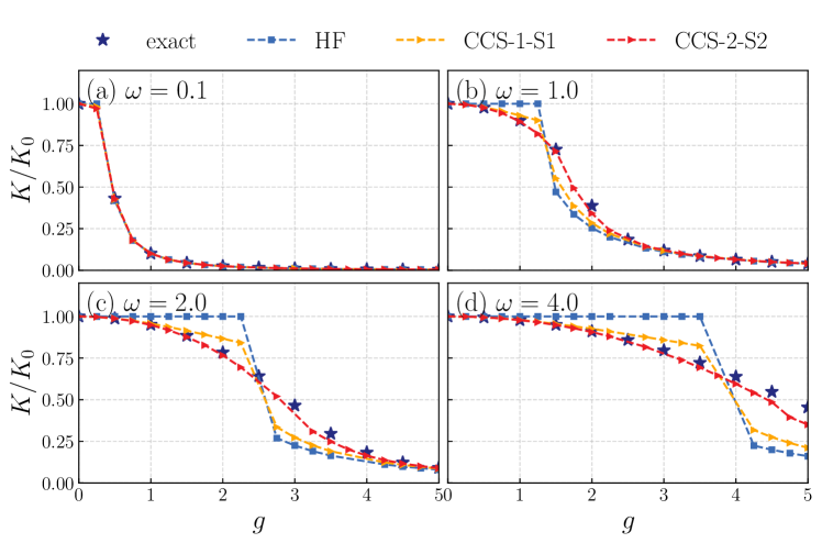
The ratio of the electron kinetic energy () to its kinetic energy at zero electron-phonon coupling () provides a simple way to diagnose the self-trapping transition even in an exact calculation where the ground-state density remains uniform. Fig. 4 plots as a function of the electron-phonon coupling strength in a 16-site Holstein model for the coupled cluster methods. All the methods accurately capture both the strong and weak coupling regimes. However, as previously noted, the simple mean-field method results in a discontinuity. As additional electron-phonon coupling is included, in CCS-1-S1 and CCS-2-S2, the continuity of the transition is gradually restored. Indeed, the CCS-2-S2 result is visually indistinguishable from the exact reference.
III.4 Electron-Lattice Correlation
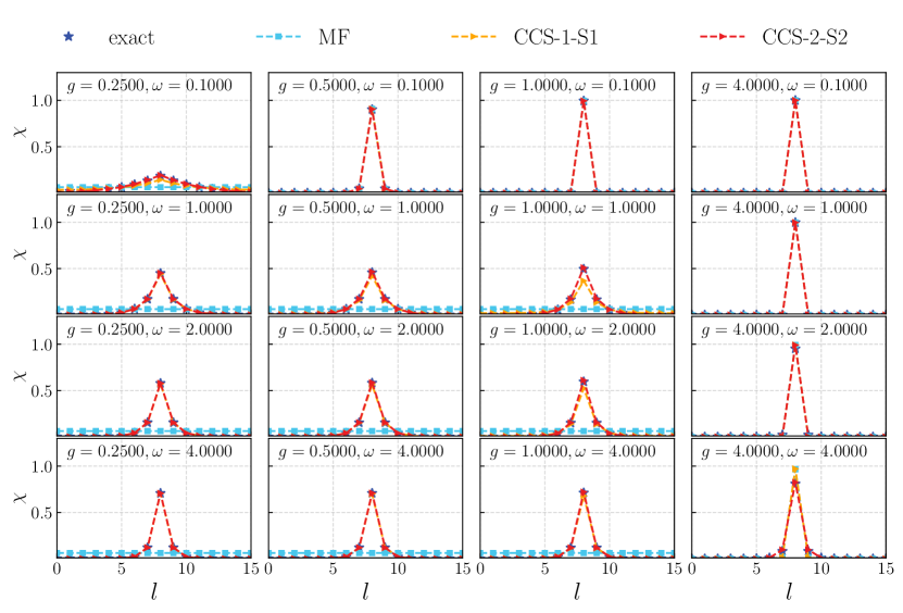
Fig. 5 displays the 16-site Holstein model’s normalized electron-lattice correlation function for various and values for the MF and CC approximations. (We choose , the middle of the lattice). Note that although the MF solution localizes the electron, there is no localization in the electron-phonon correlation function as is a product state, i.e. . As the inclusion of electron-phonon correlation increases from MF to CCS-1-S1 and CCS-2-S2, the electron-phonon correlation function becomes more compact, even as the spatial localization of the optimized reference state decreases (see Sec. III.1).
IV Conclusions
We have benchmarked the exponential ansatz across the parameter space of the Holstein model, comparing to near-exact results from DMRG. Allowing for a relaxation of the reference state that is the starting point for the exponential ansatz, we find that we can obtain a good description in the weak and strong coupling regimes, corresponding to large and small polarons. Within the systematic coupled cluster framework, increasing the electron-phonon excitation level leads to increasingly accurate results both for the energy and the correlation functions, and at the doubles level of approximation, these results are often visually indistinguishable from the exact ones. The variational Lang-Firsov transformation performs better than the lowest (i.e. singles) rung of the coupled cluster approximation hierarchy, particularly in the intermediate coupling regime.
Looking beyond models, the exponential ansatz is the starting point for a large number of applications in accurate ab initio electronic structure. The results here suggest that it is a competitive approach for polaron physics, providing a viable path forward to describe correlated electron-phonon effects at the ab initio many-body level. Another interesting direction is to examine the application of exponential wavefunctions such as the coupled cluster hierarchy to systems of many-electrons and phonons, along the lines first discussed in Ref. [25]. The incorporation of more flexible references, such as superconducting states, is of particular interest there.
Acknowledgements.
This work was supported by the U.S. Department of Energy, Office of Science, Office of Advanced Scientific Computing Research and Office of Basic Energy Sciences, Scientific Discovery through Advanced Computing (SciDAC) program under Award Number DE-SC0022088. We thank Shuoxue Li and Yao Luo for helpful discussion; and Dr. Alec White for providing valuable assistance in utilizing the Wick package. Data and codes used in this work can be obtained in https://github.com/yangjunjie0320/exp-ansatz-holstein-model.Appendix A Density Matrix Renormalization Group Theory
The density matrix renormalization group (DMRG) is a numerically exact method for solving the quantum many-body problem. The method is particularly accurate and efficient for one-dimensional systems [37, 38]. In early developments, DMRG was applied to the Holstein model in Ref. [7] to calculate the ground state energy and the electron-lattice correlation function, and to calculate the dynamical properties of the Holstein model [39]. From a modern perspective, the DMRG method is based on the matrix product state (MPS) representation of the coefficients in Eq. 2,
| (21) |
in which and are matrices with a maximum bond dimension , representing the electronic () and phonon () degrees of freedom in the site basis, respectively. The Hamiltonian is first transformed to the shifted-phonon basis of the lowest mean-field state of Eq. 4, corresponding to
| (22) |
and this Hamiltonian is expressed as a matrix product operator (MPO) in the site basis, with,
| (23) |
We then optimize the energy expectation value,
| (24) |
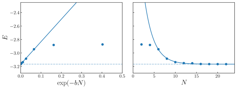
and converge our calculations with respect to the bond dimension and (shifted) phonon cutoff . Fig. 6 shows the ground state energy of the 64-site Holstein model with respect to the phonon cutoff for and . The energy is extrapolated to the infinite phonon cutoff limit using the function , where is the extrapolated energy. The bond dimension was kept at for both electron and boson sites. The electron-phonon DMRG implementation is available through the Block2 package [27, 28].
References
- Wellein and Fehske [1998] G. Wellein and H. Fehske, Self-trapping problem of electrons or excitons in one dimension, Phys. Rev. B 58, 6208 (1998).
- Landau [1933] L. Landau, Electron Motion in Crystal Lattices, Phys. Z. Sowjet. 3, 664 (1933).
- Holstein [1959] T. Holstein, Studies of polaron motion, Annals of Physics 8, 325 (1959).
- Gerlach and Löwen [1991] B. Gerlach and H. Löwen, Analytical properties of polaron systems or: Do polaronic phase transitions exist or not?, Rev. Mod. Phys. 63, 63 (1991).
- Zhang et al. [1998] C. Zhang, E. Jeckelmann, and S. R. White, Density Matrix Approach to Local Hilbert Space Reduction, Phys. Rev. Lett. 80, 2661 (1998).
- Dagotto [1994] E. Dagotto, Correlated electrons in high-temperature superconductors, Rev. Mod. Phys. 66, 763 (1994).
- Jeckelmann and White [1998] E. Jeckelmann and S. R. White, Density-matrix renormalization-group study of the polaron problem in the Holstein model, Phys. Rev. B 57, 6376 (1998).
- La Magna and Pucci [1996] A. La Magna and R. Pucci, Variational study of the discrete Holstein model, Phys. Rev. B 53, 8449 (1996).
- Brown et al. [1997] D. W. Brown, K. Lindenberg, and Y. Zhao, Variational energy band theory for polarons: Mapping polaron structure with the global-local method, J. Chem. Phys. 107, 3179 (1997).
- Romero et al. [1999a] A. H. Romero, D. W. Brown, and K. Lindenberg, Self-trapping line of the Holstein molecular crystal model in one dimension, Phys. Rev. B 60, 4618 (1999a).
- Romero et al. [1999b] A. H. Romero, D. W. Brown, and K. Lindenberg, Polaron effective mass, band distortion, and self-trapping in the Holstein molecular-crystal model, Phys. Rev. B 59, 13728 (1999b).
- Wang et al. [2020] Y. Wang, I. Esterlis, T. Shi, J. I. Cirac, and E. Demler, Zero-temperature phases of the two-dimensional Hubbard-Holstein model: A non-Gaussian exact diagonalization study, Phys. Rev. Research 2, 043258 (2020).
- Gogolin [1982] A. A. Gogolin, The Spectrum of an Intermediate Polaron and Its Bound States with Phonons at Strong Coupling, phys. stat. sol. (b) 109, 95 (1982).
- Lang and Firsov [1963] I. G. Lang and Yu. A. Firsov, Kinetic Theory of Semiconductors with Low Mobility, Sov. J. Exp. Theor. Phys. 16, 1301 (1963).
- Stephan [1996] W. Stephan, Single-polaron band structure of the Holstein model, Phys. Rev. B 54, 8981 (1996).
- Sio et al. [2019] W. H. Sio, C. Verdi, S. Poncé, and F. Giustino, Polarons from First Principles, without Supercells, Phys. Rev. Lett. 122, 246403 (2019).
- Lee et al. [2021] N.-E. Lee, H.-Y. Chen, J.-J. Zhou, and M. Bernardi, Facile ab initio approach for self-localized polarons from canonical transformations, Phys. Rev. Materials 5, 063805 (2021).
- Luo et al. [2022] Y. Luo, B. K. Chang, and M. Bernardi, Comparison of the canonical transformation and energy functional formalisms for ab initio calculations of self-localized polarons, Phys. Rev. B 105, 155132 (2022).
- Coester [1958] F. Coester, Bound states of a many-particle system, Nucl. Phys. 7, 421 (1958).
- Čížek [1966] J. Čížek, On the correlation problem in atomic and molecular systems. Calculation of wavefunction components in Ursell-Type expansion using Quantum-Field theoretical methods, J. Chem. Phys. 45, 4256 (1966).
- Paldus and Čížek [1975] J. Paldus and J. Čížek, Time-independent diagrammatic aproach to perturbation theory of fermion systems., Adv. Quantum Chem. 9, 105 (1975).
- Čížek and Paldus [1980] J. Čížek and J. Paldus, Coupled cluster approach, Phys. Scr. 21, 251 (1980).
- Bartlett and Musiał [2007] R. J. Bartlett and M. Musiał, Coupled-cluster theory in quantum chemistry, Rev. Mod. Phys. 79, 291 (2007).
- Shavitt and Bartlett [2009] I. Shavitt and R. J. Bartlett, Many-Body Methods in Chemistry and Physics: MBPT and Coupled-Cluster Theory (Cambridge University Press, New York, 2009).
- Gao et al. [2020] Y. Gao, Q. Sun, J. M. Yu, M. Motta, J. McClain, A. F. White, A. J. Minnich, and G. K. L. Chan, Electronic structure of bulk manganese oxide and nickel oxide from coupled cluster theory, Phys. Rev. B 101, 1 (2020), arxiv:1910.02191 .
- Cui et al. [2024] Z.-H. Cui, A. Mandal, and D. R. Reichman, Variational Lang–Firsov Approach Plus Møller–Plesset Perturbation Theory with Applications to Ab Initio Polariton Chemistry, J. Chem. Theory Comput. 20, 1143 (2024).
- Zhai and Chan [2021] H. Zhai and G. K.-L. Chan, Low communication high performance ab initio density matrix renormalization group algorithms, J. Chem. Phys. 154, 224116 (2021).
- Zhai et al. [2023] H. Zhai, H. R. Larsson, S. Lee, Z.-H. Cui, T. Zhu, C. Sun, L. Peng, R. Peng, K. Liao, J. Tölle, J. Yang, S. Li, and G. K.-L. Chan, Block2: A comprehensive open source framework to develop and apply state-of-the-art DMRG algorithms in electronic structure and beyond, The Journal of Chemical Physics 159, 234801 (2023).
- Alexandrov et al. [1994] A. S. Alexandrov, V. V. Kabanov, and D. K. Ray, From electron to small polaron: An exact cluster solution, Phys. Rev. B 49, 9915 (1994).
- Marsiglio [1995] F. Marsiglio, Pairing in the Holstein model in the dilute limit, Physica C: Superconductivity 244, 21 (1995).
- White et al. [2020] A. F. White, Y. Gao, A. J. Minnich, and G. K.-L. Chan, A coupled cluster framework for electrons and phonons, J. Chem. Phys. 153, 224112 (2020).
- Mordovina et al. [2020] U. Mordovina, C. Bungey, H. Appel, P. J. Knowles, A. Rubio, and F. R. Manby, Polaritonic coupled-cluster theory, Phys. Rev. Res. 2, 1 (2020), arxiv:1909.02401 .
- Haugland et al. [2020] T. S. Haugland, E. Ronca, E. F. Kjønstad, A. Rubio, and H. Koch, Coupled Cluster Theory for Molecular Polaritons: Changing Ground and Excited States, Phys. Rev. X 10, 041043 (2020).
- Li and Zhang [2023] X. Li and Y. Zhang, First-principles molecular quantum electrodynamics theory at all coupling strengths (2023), arxiv:2310.18228 [physics] .
- Yang et al. [2020] C. Yang, J. Brabec, L. Veis, D. B. Williams-Young, and K. Kowalski, Solving Coupled Cluster Equations by the Newton Krylov Method, Front. Chem. 8, 590184 (2020).
- Knoll and Keyes [2004] D. Knoll and D. Keyes, Jacobian-free Newton–Krylov methods: A survey of approaches and applications, Journal of Computational Physics 193, 357 (2004).
- White et al. [1989] S. R. White, D. J. Scalapino, R. L. Sugar, E. Y. Loh, J. E. Gubernatis, and R. T. Scalettar, Numerical study of the two-dimensional Hubbard model, Phys. Rev. B 40, 506 (1989).
- White [1993] S. R. White, Density-matrix algorithms for quantum renormalization groups, Phys. Rev. B 48, 10345 (1993).
- Zhang et al. [1999] C. Zhang, E. Jeckelmann, and S. R. White, Dynamical properties of the one-dimensional Holstein model, Phys. Rev. B 60, 14092 (1999).