Ponderomotive electron physics captured in single-fluid extended MHD model
Abstract
The well-known ponderomotive force, arising from the interaction of matter and light, has critical implications across a broad range of fields from laser fusion and astrophysics to laser diagnostics and even pulsed-power experiments. This pseudo-potential pushes electrons, which through coulomb forces causes ion density modulations that can steepen with profound implications. When used intentionally, density modulations can be used for plasma gratings, which are essential for optical components operating in extreme conditions for next generation lasers. They can also be important for plasma confinement and particle trapping, which can even impact magnetic confinement in fusion devices. The ponderomotive potential also leads to laser self-focusing, complicating laser diagnostics. In laser fusion, the force exacerbates challenges posed by stimulated Brillouin scattering (SBS) and crossed beam energy transfer (CBET), both of which destabilize the fusion process. It even plays an astrophysical role in the filamentation of fast radio bursts in the relativistic winds of magnetars. Since the ponderomotive force primarily effects electron dynamics, multi-fluid/particle codes or additional ansatz are required to include its effects. This paper demonstrates that by including electron effects on an ion timescale with a 1-fluid, 2-energy extended magnetohydrodynamics (XMHD) model, ponderomotive effects are also naturally present. We introduce the theory for these dynamics and demonstrate their presence with 1-D “pencil-like” simulations.
I Introduction
The ponderomotive force is described in detail in [1] and countless other papers and books since its discovery. It is a nonlinear force caused by the beating of collective plasma and light waves and has important consequences to fusion energy, laser diagnostics, astrophysics and even triggered x-pinches[2]. Ponderomotive force leads to electron and ion density modulations which eventually steepen [3, 4, 5]. It has also been presented as a source of magnetization in plasma[6, 7]. The sharp nature of these modulations can even been used to form plasma gratings[8, 9, 10, 11, 12] when the optical components must operate in extreme conditions. The rapidly proliferating high-power petawatt lasers [13] require modernization of diffraction optics, which can only withstand [14]. Even if another mechanism is used to form the plasma grating, ponderomotive effects will likely influence the lifetime of the optic. Density modulation have also been introduced as a consequence of ponderomotive laser self-focusing[15, 16] and even applied to the filamentation of fast radio bursts in the relativistic winds of magnetars[17, 18]. Additionally, the parametric instability[1] (stimulated Brillouin scattering) combined with ponderomotively driven plasma response has long been a major concern for laser fusion[19, 20, 21] and can even contribute to crossed beam energy transfer (CBET)[22, 23] which further destabilizes laser fusion.
While a magnetohydrodynamics (MHD) model cannot generally handle electron physics, it is possible to approximate electron effects on an ion time-scale using a relaxation scheme [24, 25] and extended MHD model. Usually, fast electron motion is neglected as it is not typically relevant to the MHD approximation of a plasma. However, by removing it along with the associated displacement current () from Maxwell-Ampere’s law, any hope of retaining light waves in a plasma is broken.
We will show in this paper how electron effects ion-timescale using the GOL can be retained even in 1-fluid extended MHD in the presence of an electromagnetic (EM) wave. By retaining these effects this paper shows we can recover some of the ponderomotive effects discussed above. For example, stimulated Brillouin scattering (SBS) turns an EM wave into another EM wave along with an ion acoustic wave (IAW), both of which are supported by this paper’s model. Previous work [26] has demonstrated consistency with collisional absorption of EM laser energy, as well as 2D effects [2] like filamentation and self-focusing.
We first introduce the analytic theory for ponderomotive dynamics on a 1-fluid XMHD ion-timescale. Then proceed to develop and analyze a simple 1-D simulation demonstrating a matching of the theory and computation.
To begin this analysis, we introduce the equations of extended MHD model and focus on the ponderomotive effects present in the GOL (Eq. I.1).
I.1 Redimensionalization of XMHD equations
In the framework of laser plasma interactions, we take the electromagnetic wave speed as our characteristic speed, . And using Faraday’s law, we let . And furthermore, the thermal pressure scale is , the resistivity scale , the magnetic field scale is , and the current density scale is leading to XMHD equations in dimensionless form,
| (1) |
| (2) |
| (3) |
| (4) |
which is used together with Maxwell’s equations and a quasi-neutral plasma assumption,
| (5) |
| (6) |
| (7) |
Using the previously defined characteristic scales we can also write the dimensionless GOL
| (8) | |||
Here is the electron plasma density, is the ratio of the ion mass to the electron mass, is the mass density, v is the flow speed, is the thermal pressure, j is the current density, B is the magnetic field, is the electric resistivity and is the energy density, all dimensionless. The redimensionalization of the GOL made the dimensional electron plasma frequency appear in front of all the terms connected to electron physics. Here, is electron plasma density, e is the elementary charge and is the electron mass, all dimensional.
II Ponderomotive force using of phasors
Since this work will demonstrate the existence of the ponderomotive force () within the XMHD model, we now define its form using this same non-dimensionalization.
| (9) |
The Generalized Ohm’s law is the natural starting point for ponderomotive effects as it is a simplification of the electron momentum conservation equation. It will now be rewritten in a form compatible with .
The dyadic current terms in Eq. (I.1) can be simplified as a consequence of quasi-neutrality () and a vector identity (). Additionally, this can be rewritten using another vector identity, , to yield the following relationship.
| (10) |
Eq. (10) does not alone show where originates, but it does suggest a solution. The RHS has two components - the first, , looks functionally similar to the form of in Eq. (9) and second, , is similar to the Hall term in Eq. (I.1). As is often the case with electromagnetic waves, a phasor representation of this equation turns out to be useful for expanding on this similarity. Phasors assume current density, electric and magnetic fields vary sinusoidally, , , and . Additionally, the system must have reached steady-state. Although these assumptions are not generally correct for a dynamic and complex laser-plasma system, they can be used for demonstrative purposes and for early-time simulations with no spatial gradients or non-uniformities.
With these definitions, the first part of Eq. (10) using phasors. Note that the real component of each phasor equation is implied when moving back into physical variables.
| (11) |
To simplify the second part of Eq. (10), some relationship between and must be defined. The phasor representation of Eq. (I.1) yields one valid for at least the assumptions already stated.
| (12) |
Since all the components oscillating with the same frequency as the laser are contained in the term, then for Eq. (12) to balance, the following relationship must hold.
| (13) |
This does assume ions are immobile (), which is true early in time and on the timescale of the laser oscillation. These conditions also imply , which in turn means . This relationship along with Eq. (7) implies may now be recast as a function of only . Consequently, when is combined with Eq. (11), then we completely defined Eq. (10) in phasor form.
Here we used to visually simplify Eq. (LABEL:eq:dyadic_phasor1). Additionally, we have taken an average over one laser cycle, where the indicates a variable has been averaged over the wave period. One final simplification is low-resisitivity (). This is justified since lasers rapidly heat colder plasma at early times as mentioned in prior work [26]. Substituting this simplified form of the dyadic term into the Generalized Ohm’s Law in Eq. (12), forms demonstrates how the ponderomotive term enters the Extended MHD model.
| (15) |
If we again substitute for and then put this in the form of the momentum equation, Eq. (2), then the form of in Eq. (9) is recovered.
| (16) |
The ponderomotive force is supported by XMHD through the inclusion of electron inertia and the Hall-term of the Generalized Ohm’s law. Furthermore, Eq. (16) shows the effect of this force can either be to change or to generate a static electric field or magnetic field.
To estimate the expected ion-fluid velocity for this semi-constant force, there are again some simplifying assumptions. If , then an ion velocity can be estimated for the journey from to , which corresponds to the maximum and halfway to the minimum locations of ponderomotive force. This is performed by the following integral,
| (17) |
In Eq. (17), M refers to , Z is the ionization state of the plasma and again there is a quasi-neutrality assumption to remove the density dependence. The equation represents the velocity ions would attain if traversing the distance from the highest pondermotive potential to halfway to the lowest. The integration cannot go to the minimum since actual at will likely be since there are equal and opposing forces pushing ions toward this location from both sides. The ion density and pressure are also expected to be peaked here, which suggests the simple model used in Eq. (17) is not capturing all the physics. Nevertheless, the theory in Eq. (17) can easily be compared to a simulation.
III Generation of a grating and comparison to other models
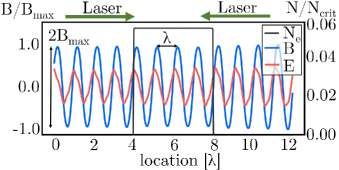
Since this work has shown a ponderomotive force is supported by single fluid XMHD, it will now be used to generate a simple ponderomotive-ion driven plasma grating. It is also prudent to see how it compares to an analytical model typical used to validate PIC models that include electrostatic fields and electron oscillations[4, 9, 10]. This section returns to dimensional equations so they are more easily associated with other works. To simplify the analysis, again limit the physics to 1-D, non-relativistic linearly s-polarized electromagnetic field. The equations are fully solved in 2D, but the resolution is fully along the x-direction, with only 9 cells in the y-direction. Furthermore, the () domain was constructed such that a standing-wave will form in a low density plasma. This simulation also uses two identical counter-propagating lasers moving along the +/- x-axis towards a low-density () plasma. The magnetic field components, , were defined on the vertical boundaries so the Poynting flux was directed to the left and right. The beam has a uniform spatial profile, . Here, , , and with . The analytic solution for the electric and magnetic fields for such a counter-propagating laser is shown below. Note that this will produce a standing wave with an amplitude 2x the incoming lasers. A snapshot of what this standing wave looks like is shown in Fig. 1.
| (18) |
When is computed using the same method as in Eq. (13) and simplifying assumptions of Eq. (15), the current in Eq. (LABEL:eq:dyadic_phasor1) can be written as,
| (19) |
The resulting Hall term in the single-fluid GOL is now easily computed using Eq. (19) and Eq. (18) for both and . As this is a source term for ion-fluid momentum conservation in Eq. (2), it really represents the effect on an ion-fluid from time-averaged electron dynamics.
| (20) |
The ponderomotive force only relates to the time-averaged Hall term (), which will bring a factor of . With an assumption that and a trigonometric identity, the time-averaged ponderomotive term of the GOL is simplified even further.
| (21) |
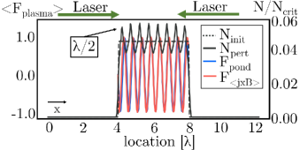
Using the simulation parameters described above, the windowed cycle-averaged was computed and plotted in Fig. 2 along with the theoretical cycled-averaged ponderomotive force (computed for the electron-fluid). Comparisons with or without resistivity included shows clearly the wave with resistivity has less symmetry than without.
Also plotted is the initial plasma density profile along with one from much later in the simulation (). The first thing to note is the theory and simulation results of the ponderomotive force agree very well. The second is there is clearly density steepening and comb-like appearance described in the earlier referenced works[8, 9, 10]. The steepening is significantly enhanced when there is resistivity present. This is likely due to easier thermalization of directed kinetic energy attained by the electrons as they wiggle in the laser field.
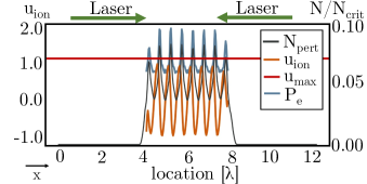
The ion velocity is the final piece of evidence to demonstrate XMHD captures the physics in Eq. (17). Fig. 3 shows simulation ion-velocity in the direction of ponderomotive force () along with from Eq. (17). The magnitude is similar, and the peak matches the earlier analytic theory, which suggested . The ion pressure and temperature also peak at as suggested earlier. This implies there will be a counterbalance to ponderomotive force at the ion peaks since . As the ponderomotive force acts on the ion fluid, the pressure continues to build and oppose a further increase in velocity.
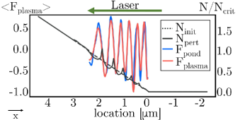
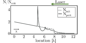
To show why ponderomotive steepening is a necessary effect to include in laser-plasma simulations, we need only look at the results of a similar simulation in Fig. 4. Here instead of using two lasers to form a standing wave, a single laser was sent from +x-axis to reflect off a steep density ramp (similar to the setup in an earlier work [4]). The reflection causes its own standing wave and ensuing ponderomotive effects.
It is clear from Fig. 4 that the effect of ponderomotive force qualitatively increases with density as earlier analytic theory suggested. Much later in time, this effect causes a supercritical steepening and plateauing of the density profile, which renders the interior of the plasma inaccessible to the laser while also potentially providing new supercritical surfaces for increased EM-reflection [3]. Both Fig. 4 and Fig. 5 show how in addition to a forward moving supercritical shock, there are possibly 1 or more supercritical density perturbations even close to the laser source. These can also capture EM radiation and increase absorption.
To verify this is a valid solution for the ions, we compare this to the ponderomotive force from theory,
| (22) |
Now we substitute our standing-wave electric field into Eq. (22) and derive a result.
| (23) |
IV Conclusion
The result in Eq. (23) exactly matches the Eq. (21) except the in the denominator and the lack of in the numerator. Ponderomotive force is not directly applied to ions with , as this would yield an extremely small force when compared with . However, we see that by using a single fluid XMHD model, we can circumvent the need to first go through an intermediate electron density displacement to get the ponderomotive force to act on an ion. Thus, we essentially assumed electrons have moved until the Coulomb force is exactly equal to the ponderomotive force on the electrons. This allows us to equate the force on the ion-fluid to the force on the electron-fluid and replace . The of the numerator is present since this ultimately a source term from the collective population of electrons. Our result matches exactly the theory and PIC simulation derived in Ref. [4], which uses a very similar setup.
We make no claims that an extended-MHD can replace or even compete with a state-of-the art hybrid-kinetic or PIC model. Instead we believe they can complement each other. Often MHD is used in applications like astro-plasma physics, z-pinch and tokamaks. These situations all generally have a well-developed fully-formed plasma for the majority of their life. It is this condition that lends itself well to MHD, and where our results here can enter. If we want to interact a laser with this type of plasma then using a model like XMHD ensures a natural crossover from LPI to MHD.
References
- Kruer [2003] W. L. Kruer, The physics of laser plasma interactions, Frontiers in physics (Boulder, Colo. [u.a.] Westview, 2003).
- Young et al. [2021] J. R. Young, M. B. Adams, H. Hasson, I. West-Abdallah, M. Evans, and P.-A. Gourdain, “Using extended MHD to explore lasers as a trigger for x-pinches,” Physics of Plasmas 28, 102703 (2021).
- Estabrook, Valeo, and Kruer [1975] K. G. Estabrook, E. J. Valeo, and W. L. Kruer, “Two-dimensional relativistic simulations of resonance absorption,” Physics of Fluids 18, 1151 (1975).
- Smith et al. [2019] J. R. Smith, C. Orban, G. K. Ngirmang, J. T. Morrison, K. M. George, E. A. Chowdhury, and W. M. Roquemore, “Particle-in-cell simulations of density peak formation and ion heating from short pulse laser-driven ponderomotive steepening,” Physics of Plasmas 26, 123103 (2019).
- Dragila and Krepelka [1978] R. Dragila and J. Krepelka, “Laser plasma density profile modification by ponderomotive force,” Journal de Physique 39, 617–623 (1978).
- Gradov and Stenflo [1983] O. Gradov and L. Stenflo, “Magnetic-field generation by a finite-radius electromagnetic beam,” Physics Letters A 95, 233–234 (1983).
- Shukla, Shukla, and Stenflo [2009] N. Shukla, P. K. Shukla, and L. Stenflo, “Magnetization of a warm plasma by the nonstationary ponderomotive force of an electromagnetic wave,” Physical Review E 80, 027401 (2009).
- Lehmann and Spatschek [2019] G. Lehmann and K. H. Spatschek, “Plasma photonic crystal growth in the trapping regime,” Physics of Plasmas 26, 013106 (2019).
- Sheng, Zhang, and Umstadter [2003] Z.-M. Sheng, J. Zhang, and D. Umstadter, “Plasma density gratings induced by intersecting laser pulses in underdense plasmas,” Applied Physics B 77, 673–680 (2003).
- Plaja and Roso [1997] L. Plaja and L. Roso, “Analytical description of a plasma diffraction grating induced by two crossed laser beams,” Physical Review E 56, 7142–7146 (1997).
- Edwards and Michel [2022] M. R. Edwards and P. Michel, “Plasma Transmission Gratings for Compression of High-Intensity Laser Pulses,” Physical Review Applied 18, 024026 (2022).
- Peng et al. [2019] H. Peng, C. Riconda, M. Grech, J.-Q. Su, and S. Weber, “Nonlinear dynamics of laser-generated ion-plasma gratings: A unified description,” Physical Review E 100, 061201 (2019).
- Danson et al. [2015] C. Danson, D. Hillier, N. Hopps, and D. Neely, “Petawatt class lasers worldwide,” High Power Laser Science and Engineering 3, e3 (2015).
- Chambonneau and Lamaignère [2018] M. Chambonneau and L. Lamaignère, “Multi-wavelength growth of nanosecond laser-induced surface damage on fused silica gratings,” Scientific Reports 8, 891 (2018).
- Kaw [1973] P. Kaw, “Filamentation and trapping of electromagnetic radiation in plasmas,” Physics of Fluids 16, 1522 (1973).
- Del Pizzo, Luther-Davies, and Siegrist [1979] V. Del Pizzo, B. Luther-Davies, and M. R. Siegrist, “Self-focussing of a laser beam in a multiply ionized, absorbing plasma,” Applied physics 18, 199–204 (1979).
- Sobacchi et al. [2023] E. Sobacchi, Y. Lyubarsky, A. M. Beloborodov, L. Sironi, and M. Iwamoto, “Saturation of the Filamentation Instability and Dispersion Measure of Fast Radio Bursts,” The Astrophysical Journal Letters 943, L21 (2023).
- Ghosh et al. [2022] A. Ghosh, D. Kagan, U. Keshet, and Y. Lyubarsky, “Nonlinear Electromagnetic-wave Interactions in Pair Plasma. I. Nonrelativistic Regime,” The Astrophysical Journal 930, 106 (2022).
- Bezzerides, Vu, and Wallace [1996] B. Bezzerides, H. X. Vu, and J. M. Wallace, “Convective gain of stimulated Brillouin scattering in long‐scale length, two‐ion‐component plasmas,” Physics of Plasmas 3, 1073–1090 (1996).
- Eliseev et al. [1995] V. V. Eliseev, W. Rozmus, V. T. Tikhonchuk, and C. E. Capjack, “Stimulated Brillouin scattering and ponderomotive self‐focusing from a single laser hot spot,” Physics of Plasmas 2, 1712–1724 (1995).
- Myatt et al. [2014] J. F. Myatt, J. Zhang, R. W. Short, A. V. Maximov, W. Seka, D. H. Froula, D. H. Edgell, D. T. Michel, I. V. Igumenshchev, D. E. Hinkel, P. Michel, and J. D. Moody, “Multiple-beam laser–plasma interactions in inertial confinement fusion,” Physics of Plasmas 21, 055501 (2014).
- Hüller et al. [2020] S. Hüller, G. Raj, W. Rozmus, and D. Pesme, “Crossed beam energy transfer in the presence of laser speckle ponderomotive self-focusing and nonlinear sound waves,” Physics of Plasmas 27, 022703 (2020).
- Ruocco [2020] A. Ruocco, Modelling of ponderomotive laser self-focusing in a plasma with a hydrodynamic code in the context of direct-drive inertial confinement fusion, phdthesis, Université de Bordeaux (2020).
- Seyler and Martin [2011] C. E. Seyler and M. R. Martin, “Relaxation model for extended magnetohydrodynamics: Comparison to magnetohydrodynamics for dense Z-pinches,” Physics of Plasmas 18, 012703 (2011).
- Martin [2010] M. R. Martin, “Generalized ohms law at the plasma-vacuum interface,” Ph. D. thesis, Cornell University (2010).
- Young and Gourdain [2024] J. R. Young and P.-A. Gourdain, “The impact of electron inertia on collisional laser absorption for high energy density plasmas,” (2024), arXiv:2310.02415 [physics].