Bridging the Gap between Partially Observable Stochastic Games and Sparse POMDP Methods

Abstract

Many real-world decision problems involve interaction of multiple self-interested agents with limited sensing ability. The partially observable stochastic game (POSG) provides a mathematical framework for posing these problems, however solving a POSG requires difficult reasoning about two critical factors: (1) information revealed by partial observations and (2) decisions other agents make. In the single agent case, partially observable Markov decision process (POMDP) planning can efficiently address partial observability with particle filtering. In the multi-agent case, extensive form game solution methods account for other agent’s decisions, but preclude belief approximation. We propose a unifying framework that combines POMDP-inspired state distribution approximation and game-theoretic equilibrium search on information sets. This paper lays a theoretical foundation for the approach by bounding errors due to belief approximation, and empirically demonstrates effectiveness with a numerical example. The new approach enables online planning in POSGs with very large state spaces, paving the way for reliable autonomous interaction in real-world physical environments and complementing offline multi-agent reinforcement learning.

1 Introduction

This paper addresses the task of online game-theoretic planning in large discrete, continuous, and hybrid state spaces with partial observability. Interaction dynamics between agents is a significant source of uncertainty in planning. This interaction can be cooperative [e.g. 1], completely opposed [e.g. 2], or the agents may have more complex relationships with competing objectives that are not completely opposed or aligned [e.g. 3]. Aside from interaction uncertainty, we also consider state uncertainty since the complete state of an environment is rarely known and must instead be inferred with incomplete and noisy observations.

The partially observable Markov decision process (POMDP) is a flexible framework that handles state uncertainty but not interaction uncertainty. Many planning methods, both online [e.g. 4, 5] and offline [e.g. 6], have been developed for solving POMDPs efficiently in practice. On the other hand, approaches from game theory focus mainly on interaction uncertainty and handle state uncertainty less robustly because they plan on the history space [e.g. 7, 8].

Some deep reinforcement learning (RL) methods [e.g. 9, 10] have enjoyed great success in environments with interaction and state uncertainty. We do not offer a comparison to these methods because they are effectively offline methods, using significant computing resources to train policies with simulated data before being tested in the environment. Our online planning approach is complementary to deep RL in several ways. For example, online planning can be used as an improvement operator during the training process [11, 12]; an online planning algorithm can act as a backbone to combine learned models for a compositional approach to planning [13]; or the structure proposed in this work could be used as an algorithmic prior for reinforcement learning algorithms [14].

The specific contributions of this paper are the following: First, after a review of background material in Section 2, Section 3 defines a tree structure, the conditional distribution information set tree (CDIT), that can accommodate both particle-based belief approximation and multi-agent reasoning. Next, Section 4 describes a counterfactual regret minimization (CFR) algorithm that finds a Nash equilibrium in the zero-sum case by exploring important parts of the CDIT. Section 5 then provides theoretical justification for the CDIT approach showing that if a Nash equilibrium is calculated using the CDIT approximation, it is likely close to a Nash equilibrium for the true game. Notably, the theoretical properties have no direct computational complexity dependence on the size of the state space. Finally, Section 6 contains a numerical experiment showing that the algorithm described in Section 4 can efficiently find effective strategies in a tag game on a continuous state space, a task that is impossible for existing methods based on POMDPs or extensive form games.

2 Background

2.1 Partially observable stochastic games

The partially observable stochastic game (POSG), also called the partially observable Markov game (POMG), is a mathematical formalism for problems where multiple agents make decisions sequentially to maximize an objective function [15, 16]. A particular finite horizon POSG instance is defined by the tuple $(\mathcal{N},\mathcal{S},\mathcal{A},\mathcal{O},\mathcal{T},\mathcal{Z},r,D,\gamma,b_{0})$, where $\mathcal{N}$ is the set of players ($i\in\mathcal{N}$) playing the game. $\mathcal{S}$ is a set of possible states; $\mathcal{A}^{i}$ is a set of player $i$’s actions; $\mathcal{O}^{i}$ is a set of player $i$’s observations; $\mathcal{T}$ is the state transition function where $\mathcal{T}(s^{\prime}|s,a)$ is the probability of transitioning from state $s$ to state $s^{\prime}$ via joint action $a$; $\mathcal{Z}^{i}$ is the observation function for player $i$ where $\mathcal{Z}^{i}(o^{i}|s,a,s^{\prime})$ is the probability that player $i$ receives observation $o^{i}$ given a transition from state $s$ to state $s^{\prime}$ via joint action $a$; $r^{i}(s,a)$ is the scalar reward function for player $i$, given state $s$ and joint action $a$; $D\in\mathbb{N}$ is the number of time steps in the horizon; $\gamma\in[0,1]$ is the discount factor; and $b_{0}$ is the initial distribution over states. The results in this paper apply to finite horizon problems. However, they can be extended to infinite-horizon discounted problems with bounded reward by choosing a horizon large enough that subsequent discounted rewards will be sufficiently small.

A policy for player $i$, $\pi^{i}$, is a mapping from that player’s action-observation history, $h^{i}$, to a distribution over actions. The space of possible polices for agent $i$ is denoted $\Pi^{i}$. A joint policy, $\pi=(\pi^{1},\pi^{2},...)$, is a collection of policies for each player. The superscript $-i$ is used to mean “all other players”. For example $\pi^{-i}$ denotes the policies for all players except $i$. Player $i$’s objective is to choose a policy to maximize his or her utility,

$$U^{i}(\pi)=\mathbb{E}_{\mathcal{T},\mathcal{Z},\pi}\left[\sum_{t=0}^{D}\gamma^{t}R^{i}(s_{t},a_{t})\mid s_{0}\sim b_{0}\right]\,.$$ (1)

Since this objective depends on the joint policy, and the reward functions for individual players may not align, POSGs are not optimization problems where locally or globally optimal solutions are always well-defined.

Instead of optima, there are a variety of possible solution concepts. The most common solution concept and the one adopted in this paper is the Nash equilibrium. A joint policy is a Nash equilibrium if every player is playing a best response to all others. Mathematically a best response to $\pi^{-i}$ is a $\pi^{i}$ that satisfies

$$U^{i}(\pi^{i},\pi^{-i})\geq U^{i}(\pi^{i\prime},\pi^{-i})$$ (2)

for all possible policies $\pi^{i\prime}$. In a Nash equilibrium, Eq. 2 is satisfied for all players.

One particularly important taxonomic feature for POSGs is the relationship between the agents’ reward functions. In cooperative games, all agents have the same reward function, $r^{i}(s,a)=r^{j}(s,a)$ for all $i$ and $j$. In a two player zero-sum game, the reward functions of the two players are directly opposed and add to zero, $r^{1}(s,a)=-r^{2}(s,a)$. When there are no restrictions on the reward function, the term general-sum is used to contrast with cooperative, zero-sum, or other special classes. The CDIT structure in Section 3 and the analysis in Section 5 are applicable to the general-sum case, while the algorithm in Section 4 applies only to the zero-sum case.

2.2 Particle filtering and tree search for POMDPs

A POMDP is a POSG special case where there is only one player. Hence, a POMDP can be described by the same tuple as a POSG, with only one action set, observation set, and conditional observation distribution for the sole player. Tree search is a scalable approach for solving POMDPs [4, 17, 5, 18]. For POMDPs, each node in the planning tree corresponds to a history, and actions are typically chosen by estimating the history-action value function, $Q(h,a)$.

A POMDP is equivalent to a belief MDP, where a belief is the state distribution conditioned on the action-observation history ($b(s)=P(s\mid h)$). As the belief is a sufficient statistic for value [19], the value function can be conditioned on beliefs instead of full histories ($Q(b,a)$). While exact Bayesian belief updates work for well for solving relatively small POMDPs [6], these methods suffer from the curse of dimensionality in large state and observation spaces. If a weighted particle filter [16] and sparse sampling [20] are used to approximate the belief MDP, there need be no direct computational dependence on the size of the state or observation spaces, breaking the curse of dimensionality [21].

2.3 Imperfect information extensive form games

Imperfect information extensive form games (EFGs) are very similar to POSGs as they both provide a model for multiagent interaction under imperfect state information. However, there are three structural differences: First, EFGs assume a sequential nature to the interaction rather than the simultaneous interaction of POSGs. Second, rather than defining a state-based reward, EFGs define rewards only for terminal action histories. Finally, instead of reasoning about observations, EFGs may arbitrarily group histories into information sets wherein a player is unable to distinguish between these histories.

One method of finding Nash equilibria in EFGs is counterfactual regret minimization (CFR) [7]. Counterfactual regret minimization extends normal form regret minimization [22] to extensive form games and has been used as a base algorithm for solving extremely large games such as heads up no limit Texas hold ’em poker [8, 23].

2.4 Limitations of POMDP and EFG approaches for physical POSGs

In physical domains such as robotics or aerospace, both POMDPs and EFGs have severe limitations. POMDP approaches are popular in robotics [24, 25], and have enjoyed success due to the many efficient methods for approximating the belief such as Kalman filtering or particle filtering. However, POMDPs are fundamentally single agent optimization problems rather than games. Cooperative POSGs, sometimes called decentralized POMDPs [26], can be solved using POMDP-based techniques [e.g. 27] since all agents seek the same goal. However, finding certain types of equilibria in general-sum games is fundamentally impossible. A simple example is a mixed Nash equilibrium: Since POMDPs always have at least one deterministic optimal policy, it is impossible for a POMDP-based approach to find an equilibrium in a game that only has a mixed Nash equilibrium. This also means that recursive POMDP-based interaction approximations such as I-POMDPs [28] cannot calculate these equilibria.

Moreover, while belief distributions are fundamentally important in POMDPs because they form the basis for many dynamic programming algorithms, they are essentially useless for POSGs. In a POSG, the state distribution conditioned on an agent’s private history also depends on the other agents’ policies, so it is impossible to calculate belief distributions without knowing these policies first. Since the very goal in a POSG is to find a joint policy that is an equilibrium, the other agents’ policies are not known a-priori, and it is not straightforward to use POMDP beliefs in intermediate steps to find POSG equilibria. Existing methods that have attempted to resolve this require exact state updates and therefore discrete state spaces [29].

Instead of belief distributions, EFG-based approaches group states into information sets without assigning probability to the set members. By deferring this probability assignment, algorithms such as CFR can find equilibria by adjusting all agents’ policies simultaneously. While the EFG formalism is general – POSGs can be represented as EFGs by modeling all uncertainty as chance player moves – it was designed for relatively simple tabletop games, and it is extremely inconvenient to model physical world domains as EFGs. More importantly, EFGs cannot easily incorporate belief approximation techniques such as Kalman filtering or particle filtering, which have been crucial in handling uncertainty in physical domains over the last half century.

3 Conditional distribution information set trees

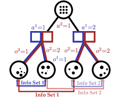
Figure 1: Illustration of a particle CDIT for a POSG with $\mathcal{A}^{1}$=$\mathcal{O}^{2}$={1,2}, $\mathcal{A}^{2}$=$\mathcal{O}^{1}$={1}.

In order to overcome the limitations above, we define a new tree structure called the conditional distribution information set tree (CDIT) that combines history-conditioned state distributions, similar to POMDP beliefs, with information sets similar to those in EFGs. A CDIT is shown in Fig. 1, which will be explained in the following sections.

3.1 Joint conditional distribution trees

The base structure of a CDIT is a joint conditional distribution tree consisting of alternating layers of joint action nodes (rectangles in Fig. 1) and joint observation nodes (unfilled circles in Fig. 1). The history for a node is the sequence of joint actions and observations on the path to that node from the root. Each depth $d$ observation node has an associated state distribution, $b_{d}$, conditioned on the history up to that point, that is

$$b_{d}(s_{d})=P(s_{d}\mid h_{d})=P(s_{d}\mid b_{0},a_{0},o_{1},...a_{d-1},o_{d})\text{.}$$ (3)

This distribution can be calculated exactly using Bayes’ rule:

$$b_{d}(s_{d})=Z(o_{d}\mid a_{d-1},s_{d})\sum_{s_{d-1}}T(s_{d}\mid s_{d-1},a_{d-1})\,b_{d-1}(s_{d-1})\,,$$ (4)

where $a_{d-1}$ is the joint action for the parent node and $b_{d-1}$ is the joint conditional distribution for the grandparent node. However, CDITs are most scalable when this belief is approximated. Any approximation, for example an extended Kalman filter or Gaussian mixture model can be used, but this work focuses on a particle CDITs, where each distribution is represented by $C$ particles (filled circles in Fig. 1):

$$\bar{b}_{d}=\{(s_{d,i},w_{d,i})\}_{i=1}^{C}.$$ (5)

Particles are propagated by sampling the joint transition distribution $s_{d+1,i}\sim\mathcal{T}(s_{d+1,i}\mid s_{d,i},a)$, and particle weights are updated according to observation probability: $w_{d+1,i}=w_{d,i}\cdot\mathcal{Z}(o\mid a,s_{d+1,i})$.

3.2 Combining joint conditional distributions with information sets

Since the distributions in the tree described above are conditioned on joint histories, they contain more information than any one player has at a given depth. In order to limit the information that policies can be conditioned on, distribution nodes corresponding to histories that are indistinguishable to a player are grouped together into information sets for each player. Specifically, two joint observation nodes are in the same information set for player $i$ if all of the actions and observations for player $i$ in the history leading up to that node are identical. This grouping is similar to the information set concept in EFGs. However, while EFGs may arbitrarily group states into information sets, by definition CDITs group nodes according to the criterion above.

The combination of a joint conditional distribution tree and history-based information sets constitutes a CDIT. Figure 1 shows the first two layers of a particle CDIT for a simple example. The root node contains particles sampled from $b_{0}$. Since Player 1 has two actions an Player 2 only has one action, there are two joint action nodes, and since Player 1 has only one observation and Player 2 has two observations, there are two observation children for each action node. This yields four state distributions in the bottom layer with particles sampled using $\mathcal{T}$ and weighted with $\mathcal{Z}$. At this level, each player has two information sets. For Player 1, the left two nodes are grouped into an information set corresponding to $(a^{1}=1,o^{1}=1)$, and the right two are grouped into a set corresponding to $(a^{1}=2,o^{1}=1)$. For Player 2, the first and third nodes are grouped into the $(a^{2}=1,o^{2}=1)$ set and the second and fourth are grouped into the $(a^{2}=1,o^{2}=2)$ set.

4 Finding approximate Nash equilibria on CDITs with ESCFR

While the CDIT provides a suitable structure for approximating a POSG, an equilibrium-finding algorithm is needed to solve it. This section describes a particular algorithm, external sampling counterfactual regret minimization (ESCFR) that can find Nash equilibria for zero sum games.

Counterfactual regret minimization (CFR) algorithms reason using counterfactual action utilities:

$$q_{i,c}^{\pi}(I,a)=\sum_{h\in I}P^{\pi}_{-i}(h)q_{i}^{\pi}(h,a),$$ (6)

where $P^{\pi}_{-i}(h)$ is the counterfactual reach probability of history $h$ for player $i$, and $q_{i}^{\pi}(h,a)$ is the non-counterfactual history-action value. Counterfactual reach probability stems from the ability to factor reach probability into player components i.e. $P^{\pi}(h)=P^{\pi}_{i}(h)\cdot P^{\pi}_{-i}(h)$. The counterfactual reach probability can then be interpreted as the probability that history $h$ is reached supposing that all players play according to the strategy $\pi$ except player $i$ who plays to reach $h$. The history-action value is given by

$$q_{i}^{\pi}(h,a)=\mathbb{E}_{\pi^{-i},\mathcal{T},\mathcal{Z}}\left[r^{i}(h,a)+\gamma v^{\pi}_{i}(h^{\prime}=hao)\right]\text{,}$$ (7)

where $v_{i}^{\pi}(h)=\sum_{a_{i}\in\mathcal{A}_{i}}\pi_{i}(h,a)q_{i}^{\pi}(h,a)$. However, for particle filter CDITs, the counterfactual reach probabilities $P^{\pi}_{-i}(h)$ become nontrivial to compute. These quantities depend on players’ policies $\pi_{i}$ as well as environmental factors $(\mathcal{T},\mathcal{Z})$. As such, the probability of transitioning from history $h$ to history $h^{\prime}=hao$ is given by

$$P^{\pi}(h^{\prime}=hao|h)=p(o|h,a)\cdot\Pi_{i\in\mathcal{N}}\pi_{i}(I_{i}(h),a_{i})$$ (8)

Here $p(o\mid h,a)$ is analogous to the “chance player” policy for EFGs. In a particle CDIT, the probability of an observation given some particle belief $\bar{b}_{d}$ and joint action $a$ is

$$p(o\mid\bar{b}_{d},a)=\frac{\sum_{i=1}^{C}w_{d,i}\cdot[\int_{S}\mathcal{Z}(o\mid a,s^{\prime})\mathcal{T}(s^{\prime}\mid s_{d,i},a)ds^{\prime}]}{\sum_{i=1}^{C}w_{d,i}}.$$ (9)

However, computing this quantity is generally very difficult or even impossible. This necessitates external sampling [30] where a sampled regret $\tilde{r}$ is accumulated

$$\tilde{r}^{i}(I,a)=(1-\pi(I,a))\sum_{h\in Q_{I}}q^{\pi}_{i}(h,a),$$ (10)

where $Q_{I}$ denotes the subset of histories in information state $I$ that have been sampled. As such, no reach probabilities need to be explicitly recorded, sidestepping the necessity to compute intractible integral given in Eq. 9.

5 Convergence guarantees for approximate Nash equilibria on CDITs

When using a particle CDIT to approximate a game, a crucial question is whether equilibria computed on the CDIT, for example with the ESCFR algorithm above, converge to equilibria in the original game as the number of particles increases. This section answers that question affirmatively. Although the bounds in this section are extremely loose, they show that the approach is sound. Moreover, unlike the previous section which focused on zero-sum games, these results apply to general sum games, and the bounds have no direct dependence on the size of the state space, suggesting that the general approach can scale to large state spaces.

We separate the convergence guarantees into three parts. First, we show that the suboptimality of a solution calculated using an approximate game is bounded when applied to the true game in Section 5.1. Then, we bound utility approximation error of this approximate game in Section 5.2. Next, we show that using a sampled subset of the strategies and observations in the approximate game is sufficient to solve the approximate game in Section 5.3. Finally, we bound the suboptimality of a sparse ESCFR solution in Section 5.4.

5.1 Suboptimality of Approximate Game

A CDIT yields an approximate estimate of the utility function $\hat{U}(\pi)$. Since this estimate differs from the true utility, $U(\pi)$, we must characterize how equilibria computed with $\hat{U}(\pi)$ are related to equilibria on the original game. To do this, we use a normal form game where each action corresponds to a pure policy for a subset of the players in the original POSG. Specifically, this game is defined by a set of $|\mathcal{N}|$ payoff matrices, $A$, with each player’s payoff matrix denoted $A^{i}$. The payoff matrix entries for the true and approximated games are defined as

$$A^{i}_{j,k}\equiv U^{i}(\sigma^{i}_{j},\sigma^{-i}_{k})\qquad\text{and}\qquad\hat{A}^{i}_{j,k}\equiv\hat{U}^{i}(\sigma^{i}_{j},\sigma^{-i}_{k})$$ (11)

where $\sigma^{i}_{j}$ is the $j$th pure policy played by player $i$ and $\sigma^{-i}_{k}$ is the $k$th joint policy between all players that are not player $i$. By considering mixtures of the pure strategies in this normal form game, we consider all mixed strategies in the POSG since POSGs inherently have perfect recall and thus Kuhn’s theorem applies [31].

A Nash equilibrium requires that no player has incentive to deviate from their current strategy. For a game with payoff matrices $A$, we denote the value of the incentive to deviate with

$$\delta^{i}_{A}\equiv\max_{\pi^{i\prime}}\left(\pi^{i\prime\,T}A^{i}\pi^{-i}\right)-\pi^{i\,T}A^{i}\pi^{-i}.$$ (12)

The sum of deviation incentives for all players,

$$\textsc{NashConv}_{A}(\pi)=\sum_{i}\delta^{i}_{A}(\pi)\text{,}$$ (13)

will be used as a distance metric between the current strategy and a Nash equilibrium [32]. The matrix of approximation errors will be denoted with $E^{i}\equiv A^{i}-\hat{A}^{i}$. Using this notation, the following Lemma bounds the error in NashConv given payoff estimation errors.

Lemma 1.

In a game with payoff matrices $A$, the deviation incentive for Player $i$ from a policy $\pi$ can be upper bounded by

$$\delta^{i}_{A}(\pi) \leq\delta^{i}_{\hat{A}}(\pi)+\delta^{i}_{E}(\pi)$$ (14)

$$\leq\delta^{i}_{\hat{A}}(\pi)+2||E^{i}||_{\infty}\,\text{,}$$

and

$$\textsc{NashConv}_{A}(\pi) \leq\sum_{i}\left[\delta^{i}_{\hat{A}^{i}}(\pi)+2||E^{i}||_{\infty}\right].$$ (15)

The proof for Lemma 1 is in Appendix A. The proof relies on the ability to upper bound best response utility in normal form by the sum of maximizations upper bounding a maximization over a sum.

5.2 Particle CDIT Policy Evaluation Error

We now turn our attention to bounding the error in the particle CDIT utility estimate, $\hat{U}$. It should be noted that evaluating a joint policy on the joint conditional distribution tree core of a CDIT is functionally identical to evaluating a POMDP policy. As such, we can invoke recently-developed utility approximation error bounds for particle filter approximation in POMDPs [21, 33]:

Theorem 1.

Assume that the immediate state reward estimate is probabilistically bounded such that $P(|r_{j}^{k}-\tilde{r}_{j}^{k}|\geq\nu)\leq\delta_{r}(\nu,N_{r})$, for a number of reward samples $N_{r}$ and state sample $x_{k}^{j}$. Assume that $\delta_{r}(\nu,N_{r})\rightarrow 0$ as $N_{r}\rightarrow\infty$. For all policies $\sigma\in\Sigma,t=0,...,D$, and $a\in A$, the following bounds hold with probability of at least $1-5(4C)^{D+1}(\exp(-C\cdot\acute{k}_{i}^{2})+\delta_{r}(\nu,N_{r}))$:

$$\left|U^{i}(\sigma)-\hat{U}^{i}(\sigma)\right|\leq\alpha_{0}+\beta_{0}=||E^{i}||_{\infty},$$ (16)

where

$$\alpha_{t}=(1+\gamma)\lambda+\gamma\alpha_{t+1},\,\alpha_{L}=\lambda\geq 0,$$ (17)

$$\beta_{t}=2\nu+\gamma\beta_{t+1},\,\beta_{L}=2\nu\geq 0$$ (18)

$$k_{\max,i}(\lambda,C)=\frac{\lambda}{4V_{\max,i}d_{\infty}^{\max}}-\frac{1}{\sqrt{C}}>0,$$ (19)

$$\acute{k}_{i}=\min\left\{k_{\max,i},\lambda/4\sqrt{2}V_{\max,i}\right\}.$$ (20)

Proof.

(Sketch) This follows immediately from Theorem 3 of Lev-Yehudi et al. [33] applied to the root node of a joint conditional distribution tree at $t=0$ using a deterministic joint policy $\sigma$. A more detailed account is given in Appendix C. ∎

5.3 Surrogate Game Sufficiency

For a particle CDIT, we need only consider a subset of the full policy space. We call this restricted subspace of the full policy space the "surrogate" policy space, denoted by $\Sigma_{s}$. We consider two policies "tree-equivalent" if they take all of the same actions in all beliefs sampled in the tree.

More formally, sparse sampling-$\omega$-$\pi$ constructs a tree that samples a subset of the total history space $\mathcal{H}_{\omega\pi}\subseteq\mathcal{H}$. Any two deterministic policies $\sigma^{A},\sigma^{B}$ are tree-equivalent if $\sigma^{A}(h)=\sigma^{B}(h)\,\forall h\in\mathcal{H}_{\omega\pi}$. We consider a basis set of policies for the surrogate approximate game $\Sigma_{s}$ of size $(|A|\cdot C)^{D}$, where $\forall h\in\mathcal{H}_{\omega\pi},a\in A,\exists\sigma_{s}\in\Sigma_{s}\text{ s.t. }\sigma_{s}(h)=a$. For completeness each policy $\sigma_{s}\in\Sigma_{s}$ falls back to an arbitrary fixed default policy $\sigma_{\text{default}}$ for all $h\notin\mathcal{H}_{\omega\pi}$.

Given that the size of the true policy space is larger than the size of the surrogate policy space, we can construct a bijective mapping between the true policy space and the tree-equivalent surrogate policy space.

$$\phi:\Sigma\rightarrow\Sigma_{s}$$ (21)

$$\phi(\sigma)=\sigma_{s}\in\Sigma_{s}\text{ s.t. }\sigma(h)=\sigma_{s}(h)\,\forall h\in\mathcal{H}_{\omega\pi}$$ (22)

Lemma 2.

Two tree-equivalent policies yield the same utility when evaluated with the same sparse-sampling-$\omega$-$\pi$ tree.

Proof.

By definition, two tree-equivalent policies ($\sigma_{1},\sigma_{2}$) have $\sigma_{1}(h_{t})=\sigma_{2}(h_{t})\,\forall h_{t}\in\mathcal{H}_{\omega\pi}$. Again, by definition, a sparse-sampling-$\omega$-$\pi$ tree only evaluates histories $h_{t}\in\mathcal{H}_{\omega\pi}$. If the evaluated histories are identical, and the actions taken by policies in these histories are identical, then the policy values yielded by sparse-sampling-$\omega$-$\pi$ are also identical.

∎

Lemma 3.

In an approximate particle CDIT, a player has no incentive to unilaterally deviate to a strategy not in the considered surrogate policy space.

Proof.

In Appendix. ∎

Theorem 2.

The following bound holds with probability of at least $1-5|\mathcal{N}||\Pi|(4C)^{D+1}(\exp(-C\cdot\acute{k}_{i}^{2})+\delta_{r}(\nu,N_{r}))$:

$$\textsc{NashConv}^{A}(\pi)\leq\sum_{i\in\mathcal{N}}\left[\delta_{i,s}^{\hat{A}^{i}}(\pi)+2||E^{i}||_{\infty}\right],$$ (23)

where,

$$||E^{i}||_{\infty}=\alpha_{0}+\beta_{0}$$ (24)

$\alpha_{t},\beta_{t},\acute{k}$ are defined in Theorem 2.

Proof.

From Lemma 1, we know that

$$\textsc{NashConv}_{A}(\pi)\leq\sum_{i}\left[\delta^{i}_{\hat{A}^{i}}(\pi)+2||E^{i}||_{\infty}\right]\,,$$ (25)

where $\hat{A}^{i}$ is a game considering the full policy space.

From Lemma 3, we find that $\delta_{i,s}^{\hat{A}^{i}}(\pi)=\delta_{i}^{\hat{A}^{i}}(\pi)$, indicating that we need only consider the smaller surrogate policy space $\Sigma_{s}$, leading to the following suboptimality bound

$$\textsc{NashConv}^{A}(\pi)\leq\sum_{i\in\mathcal{N}}\left[\delta_{i,s}^{\hat{A}^{i}}(\pi)+2||E^{i}||_{\infty}\right]\,.$$ (26)

From Theorem 1, we know that utility approximation error for any policy $\sigma$ given the reward function for player $i$, and the rest of the constants follow directly from this theorem.

While Theorem 1 produces a probabilistic bound relevant to a single policy and a single player’s reward function, this bound must now hold for all players and all possible joint policies. As such, a union bound is applied to the satisfaction probability of Theorem 1 over all policies and all players, yielding a multiplicative factor of $|\mathcal{N}||\Pi|$. Here $|\mathcal{N}|$ is the number of players and $|\Pi|=\sum_{t=0}^{D}(|\mathcal{A}|\cdot|\mathcal{O}|)^{d}$ is the number of possible joint closed-loop policies. ∎

Naturally, for Theorem 2 to hold, the number of $D$-step policies must be finite, consequently requiring that both $\mathcal{A}$ and $\mathcal{O}$ also be finite sets.

5.4 ESCFR Full Game Convergence

Theorem 3.

For two-player zero-sum games, the following bound holds with probability of at least $1-2[p+5|\Pi|(4C)^{L+1}(\exp(-C\cdot\acute{k}^{2})+\delta_{r}(\nu,N_{r}))]$:

$$\textsc{NashConv}^{A}(\pi)\leq 4(\epsilon+||E||_{\infty})$$ (27)

where,

$$\epsilon=\left(1+\frac{\sqrt{2}}{\sqrt{p}}\right)\frac{\max_{i}\left[\Delta_{u,i}M_{i}\sqrt{|A_{i}|}\right]}{2\sqrt{T}}$$ (28)

$$||E||_{\infty}=\alpha_{0}+\beta_{0}$$ (29)

$\alpha_{t},\beta_{t},\acute{k}$ are defined in Theorem 2.

Proof.

For a given player $i$, average overall regret of ESCFR is bounded by

$$R_{i}^{T}\leq\left(1+\frac{\sqrt{2}}{\sqrt{p}}\right)\frac{\Delta_{u,i}M_{i}\sqrt{|A_{i}|}}{\sqrt{T}}\,,$$ (30)

with probability $1-p$ after $T$ ESCFR iterations [30]. Here, $R_{i}^{T}$ denotes the bounded average overall regret, and $T$ denotes the number of CFR iterations performed. $\Delta_{u,i}$ denotes the range of terminal utilities to player $i$. For EFGs this utility is realized purely at the terminal histories of the game. However, for the POSGs that we consider, reward is accumulated, and the EFG-equivalent terminal utility is the discounted sum of expected rewards of a given history. $A_{i}$, in this case is the set of all player $i$ action history subsequences. For POSGs this is simply $|\mathcal{A}_{i}|^{D}$. $M_{i}=\sum_{a_{i}\in A_{i}}\sqrt{|\mathcal{I}_{i}(a_{i})|}$, where $\mathcal{I}_{i}(a_{i})$ is the set of all information sets where player $i$’s action sequence up to that information set is $a_{i}$.

For the finite horizon problems we consider, $\Delta_{u,i}$ can be expressed as a finite geometric sum of rewards

$$\Delta_{R,i} =\max_{s,a}R^{i}(s,a)-\min_{s,a}R^{i}(s,a)$$ (31)

$$\Delta_{u,i} =\frac{\Delta_{R,i}(1-\gamma^{D})}{1-\gamma}$$

In a zero-sum game, if $R_{i}^{T}\leq\epsilon$, then average strategy $\bar{\sigma}^{T}$ is a $2\epsilon$ equilibrium.

$$u_{i}(\sigma_{i},\sigma_{-i})\geq u_{i}(\sigma_{i}^{\prime},\sigma_{-i})-\epsilon,\,\forall i\in\mathcal{N},\sigma_{i}^{\prime}\in\Sigma_{i}$$ (32)

By definition of $\delta$ and $\epsilon$, we have $\forall i\in\mathcal{N}\,\delta^{i}\leq\epsilon$ as well as $\epsilon\leq\max_{i\in\mathcal{N}}\delta^{i}$. In a zero-sum game, if $R_{i}^{T}\leq\epsilon$ for all players, then average strategy $\pi^{T}$ is a $2\epsilon$ equilibrium. Consequently,

$$\epsilon\leq\max_{i}R_{i}^{T}/2=\left(1+\frac{\sqrt{2}}{\sqrt{p}}\right)\frac{\max_{i}\left[\Delta_{u,i}M_{i}\sqrt{|A_{i}|}\right]}{2\sqrt{T}}\,,$$ (33)

with probability $1-2p$ due to a union bound over regret bound satisfaction probability for both players.

We combine this bound for $\delta^{i}$ specific to ESCFR with the suboptimality bound in Theorem 2. The satisfaction probability of this final bound is the result of a union bound over the satisfaction probabilities of ESCFR regret bounds and policy value error bounds. ∎

6 Numerical experiments

To demonstrate the effectiveness of our solver, we construct a game of tag in 2-dimenstional continuous state space for each agent (4 dimensions total) with discrete finite actions and observations. A pursuer and an evader start in positions uniformly randomly sampled from $b_{0}=\mathcal{U}[-0.25,0.25]\times\mathcal{U}[-0.25,0.25]$. Each agent observes the quadrant the other agent’s relative position is in. Both agents can move in 4 cardinal directions. The pursuer only receives a reward of 1 once coming within a radius of 0.1 of the evader. As this is a zero-sum game, $r^{\text{pursuer}}(s,a)=-r^{\text{evader}}(s,a)$.

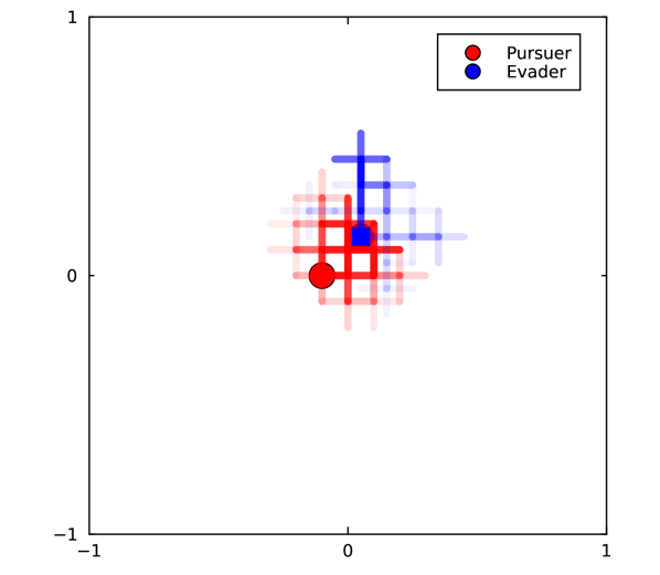
(a) Policies marginalized over observations.

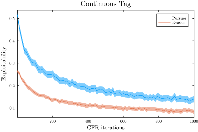
(b) Exploitability; $3\sigma$ standard error bounds shaded.

Figure 2: Numerical experiment results for continuous tag game.

To elucidate the adversarial nature of the interaction uncertainty in these zero-sum games, we quantify suboptimality via exploitability, which we define to be how much utility an opponent is able to take away i.e. $e^{i}(\pi)=v^{i}(\pi)-\min_{\pi^{-i}}v^{i}(\pi^{i},\pi^{-i})$. For Player $i$, this is equivalent to $\delta^{-i}$, and thus the sum of exploitabilities is equivalent to NashConv in two-player zero-sum games.

To solve the game of continuous tag, we construct and solve a particle CDIT up to 5 time steps with beliefs consisting of 100 particles and 1000 total ESCFR iterations. Figure 2(a) shows a policy found by ESCFR marginalized over possible observations. More opaque lines show more likely trajectories. It is clear that this policy is highly stochastic, indicating that both agents are engaging in deception that would be impossible for a POMDP planner. To estimate exploitability of an ESCFR policy, POMCP [4] is used as a best-responder. Due to the stochasticity in tree construction and ESCFR solution, the game is solved 100 times to generate the mean and $3\sigma$ standard error exploitability curves displayed in Fig. 2(b). Experiments used Julia [34] on a 2020 MacBook Air with 16GB RAM in approximately 20 minutes with 2x multiprocessing.

7 Conclusion

This paper proposes a new approach for solving partially observable stochastic games by combining imperfect information game solution methodology with distribution approximations developed for POMDPs. This combination advances the state-of-the-art in POSG solutions by extending solutions to continuous state spaces and large observation spaces, providing low-exploitability solutions with high probability. While the results do indeed show that suboptimality is bounded, the bound is loose and conservative, especially with the included union bound over the size of the policy space. In future research, we aim to extend these approximate solution methods to fully continuous observation spaces while retaining convergence guarantees and scale up the solutions by integrating online planning and offline learning.

Appendix

Appendix A Proof of Lemma 1

Proof.

$$\delta_{i}^{A}(\pi) =\max_{\pi_{i}^{\prime}}\left(\pi_{i}^{\prime T}A\pi_{-i}\right)-\pi_{i}^{T}A\pi_{-i}$$ (34)

$$=\max_{\pi_{i}^{\prime}}\left(\pi_{i}^{\prime T}(\hat{A}+E)\pi_{-i}\right)-\pi_{i}^{T}(\hat{A}+E)\pi_{-i}$$

$$\leq\left\{\max_{\pi_{i}^{\prime}}\left(\pi_{i}^{\prime T}\hat{A}\pi_{-i}\right)-\pi_{i}^{T}\hat{A}\pi_{-i}\right\}+\left\{\max_{\pi_{i}^{\prime}}\left(\pi_{i}^{\prime T}E\pi_{-i}\right)-\pi_{i}^{T}E\pi_{-i}\right\}$$

$$=\delta_{i}^{\hat{A}}(\pi)+\delta_{i}^{E}(\pi)$$

$$\leq\delta_{i}^{\hat{A}}(\pi)+2||E||_{\infty}$$

Consequently,

$$\textsc{NashConv}_{A}(\pi)\leq\sum_{i}\left[\delta^{i}_{\hat{A}^{i}}(\pi)+2||E^{i}||_{\infty}\right].$$ (35)

∎

Appendix B Proof of Lemma 3

Proof.

Suppose we have a surrogate approximate game wherein player $i$ has desire $\delta^{i}$ to deviate. If we allow player $i$ the policy space afforded in the full approximate game, they will still only have desire $\delta^{i}$ to deviate.

$$\delta^{i}_{s}=\max_{\sigma^{i}_{s}\in\Sigma_{s}}\left[\hat{U}^{i}(\sigma^{i}_{s},\pi^{-i})\right]-\hat{U}(\pi^{i},\pi^{-i})$$ (36)

$$\hat{U}^{i}(\sigma^{i},\pi^{-i})=\sum_{\sigma^{-i}\in\Sigma^{-i}}\hat{U}(\sigma^{i},\sigma^{-i})\pi^{-i}(\sigma^{-i})$$ (37)

$$\delta^{i}=\max_{\sigma^{i}\in\Sigma}\left[\hat{U}^{i}(\sigma^{i},\pi^{-i})\right]-\hat{U}(\pi^{i},\pi^{-i})$$ (38)

By consequence of Lemma 2, we get the following relation

$$\delta^{i}-\delta^{i}_{s} =\max_{\sigma^{i}\in\Sigma}\left[\hat{U}^{i}(\sigma^{i},\pi^{-i})\right]-\max_{\sigma^{i}_{s}\in\Sigma_{s}}\left[\hat{U}^{i}(\sigma^{i}_{s},\pi^{-i})\right]$$ (39)

$$=\max_{\sigma^{i}\in\Sigma}\left[\hat{U}^{i}(\phi(\sigma^{i}),\pi^{-i})\right]-\max_{\sigma^{i}_{s}\in\Sigma_{s}}\left[\hat{U}^{i}(\sigma^{i}_{s},\pi^{-i})\right]$$

$$=\max_{\sigma^{i}_{s}\in\Sigma_{s}}\left[\hat{U}^{i}(\sigma^{i}_{s},\pi^{-i})\right]-\max_{\sigma^{i}_{s}\in\Sigma_{s}}\left[\hat{U}^{i}(\sigma^{i}_{s},\pi^{-i})\right]$$

$$=0\,.$$

Therefore, $\delta^{i}=\delta^{i}_{s}$

∎

Appendix C Proof of Theorem 1

Theorem 4.

(Theorem 3 of Lev-Yehudi et al. [33]) Assume that the immediate state reward estimate is probabilistically bounded such that $P(|r_{j}^{i}-\tilde{r}_{j}^{i}|\geq\nu)\leq\delta_{r}(\nu,N_{r})$, for a number of reward samples $N_{r}$ and state sample $x_{i}^{j}$. Assume that $\delta_{r}(\nu,N_{r})\rightarrow 0$ as $N_{r}\rightarrow\infty$. For all policies $\pi,t=0,...,L$, and $a\in A$, the following bounds hold with probability of at least $1-5(4C)^{D+1}(\exp(-C\cdot\acute{k}^{2})+\delta_{r}(\nu,N_{r}))$:

$$\left|Q_{\mathbf{P},t}^{\pi,\left[p_{Z}/q_{Z}\right]}\left(b_{t},a\right)-Q_{\mathbf{M}_{\mathbf{P}},t}^{\pi,\left[p_{Z}/q_{Z}\right]}\left(\bar{b}_{t},a\right)\right|\leq\alpha_{t}+\beta_{t}=\epsilon,$$ (40)

where

$$\alpha_{t}=(1+\gamma)\lambda+\gamma\alpha_{t+1},\,\alpha_{L}=\lambda\geq 0,$$ (41)

$$\beta_{t}=2\nu+\gamma\beta_{t+1},\,\beta_{L}=2\nu\geq 0$$ (42)

$$k_{\max}(\lambda,C)=\frac{\lambda}{4V_{\max}d_{\infty}^{\max}}-\frac{1}{\sqrt{C}}>0,$$ (43)

$$\acute{k}=\min\left\{k_{\max},\lambda/4\sqrt{2}V_{\max}\right\}.$$ (44)

While Lev-Yehudi et al. [33] further generalize particle-belief MDP policy evaluation to simplified observation models, we assume that the observation model is known. This simplifies the Rényi divergence back to the definition provided in [21], where $\mathcal{P}^{d}$ is the target distribution and $\mathcal{Q}^{d}$ is the sampling distribution for particle importance sampling.

$$d_{\infty}(\mathcal{P}^{d}||\mathcal{Q}^{d})=\operatorname*{esssup}_{x\sim\mathcal{Q}^{d}}w_{\mathcal{P}^{d}/\mathcal{Q}^{d}}(x)\leq d_{\infty}^{\max}<+\infty$$ (45)

In order to extend $V_{\max}$ from Theorem 4 to the multiagent setting, we specify that $V_{\max,i}$ bounds value for player $i$ such that

$$V_{\max,i}=\frac{\max_{s,a}|R^{i}(s,a)|(1-\gamma^{D})}{1-\gamma}\,.$$ (46)

We take the established guarantee at the root belief, and

$$U^{i}(\sigma) =Q_{\mathbf{P},0}^{\sigma,\left[p_{Z}/q_{Z}\right]}\left(b_{0},\sigma(h_{0})\right)$$ (47)

$$\hat{U}^{i}(\sigma) =Q_{\mathbf{M}_{\mathbf{P}},0}^{\pi,\left[p_{Z}/q_{Z}\right]}\left(\bar{b}_{0},\sigma(h_{0})\right)\,,$$

for a given player $i$.

References

- Lee and Lee [2021] Hyun-Rok Lee and Taesik Lee. Multi-agent reinforcement learning algorithm to solve a partially-observable multi-agent problem in disaster response. European Journal of Operational Research, 291(1):296–308, 2021.
- Becker and Sunberg [2022] Tyler Becker and Zachary Sunberg. Imperfect information games and counterfactual regret minimization in space domain awareness. The Advanced Maui Optical and Space Surveillance Technologies (AMOS) Conference, 2022.
- [3] Meta Fundamental AI Research Diplomacy Team (FAIR), Anton Bakhtin, Noam Brown, Emily Dinan, Gabriele Farina, Colin Flaherty, Daniel Fried, Andrew Goff, Jonathan Gray, Hengyuan Hu, Athul Paul Jacob, Mojtaba Komeili, Karthik Konath, Minae Kwon, Adam Lerer, Mike Lewis, Alexander H. Miller, Sasha Mitts, Adithya Renduchintala, Stephen Roller, Dirk Rowe, Weiyan Shi, Joe Spisak, Alexander Wei, David Wu, Hugh Zhang, and Markus Zijlstra. Human-level play in the game of diplomacy by combining language models with strategic reasoning. Science, 378(6624):1067–1074, 2022.
- Silver and Veness [2010] David Silver and Joel Veness. Monte-Carlo planning in large POMDPs. In Advances in Neural Information Processing Systems, pages 2164–2172, 2010. URL http://papers.nips.cc/paper/4031-monte-carlo-planning-in-large-pomdps.pdf.
- Sunberg and Kochenderfer [2018] Zachary Sunberg and Mykel Kochenderfer. Online algorithms for pomdps with continuous state, action, and observation spaces. In Proceedings of the International Conference on Automated Planning and Scheduling, volume 28, pages 259–263, 2018.
- Kurniawati et al. [2008] Hanna Kurniawati, David Hsu, and Wee Sun Lee. SARSOP: Efficient point-based POMDP planning by approximating optimally reachable belief spaces. In Robotics: Science and Systems, volume 2008, 2008.
- Zinkevich et al. [2007] Martin Zinkevich, Michael Johanson, Michael Bowling, and Carmelo Piccione. Regret minimization in games with incomplete information. Advances in neural information processing systems, 20:1729–1736, 2007.
- Moravčik et al. [2017] Matej Moravčik, Martin Schmid, Neil Burch, Viliam Lisý, Dustin Morrill, Nolan Bard, Trevor Davis, Kevin Waugh, Michael Johanson, and Michael Bowling. DeepStack: Expert-level artificial intelligence in heads-up no-limit poker. Science, 356(6337):508–513, 2017. ISSN 0036-8075. doi: 10.1126/science.aam6960. URL https://science.sciencemag.org/content/356/6337/508.
- Vinyals et al. [2019] Oriol Vinyals, Igor Babuschkin, Wojciech M. Czarnecki, Michaël Mathieu, Andrew Dudzik, Junyoung Chung, David H. Choi, Richard Powell, Timo Ewalds, Petko Georgiev, Junhyuk Oh, Dan Horgan, Manuel Kroiss, Ivo Danihelka, Aja Huang, Laurent Sifre, Trevor Cai, John P. Agapiou, Max Jaderberg, Alexander S. Vezhnevets, Rémi Leblond, Tobias Pohlen, Valentin Dalibard, David Budden, Yury Sulsky, James Molloy, Tom L. Paine, Caglar Gulcehre, Ziyu Wang, Tobias Pfaff, Yuhuai Wu, Roman Ring, Dani Yogatama, Dario Wünsch, Katrina McKinney, Oliver Smith, Tom Schaul, Timothy Lillicrap, Koray Kavukcuoglu, Demis Hassabis, Chris Apps, and David Silver. Grandmaster level in starcraft ii using multi-agent reinforcement learning. Nature, 575(7782):350–354, Nov 2019. ISSN 1476-4687. doi: 10.1038/s41586-019-1724-z. URL https://doi.org/10.1038/s41586-019-1724-z.
- Jaderberg et al. [2019] Max Jaderberg, Wojciech M. Czarnecki, Iain Dunning, Luke Marris, Guy Lever, Antonio Garcia Castañeda, Charles Beattie, Neil C. Rabinowitz, Ari S. Morcos, Avraham Ruderman, Nicolas Sonnerat, Tim Green, Louise Deason, Joel Z. Leibo, David Silver, Demis Hassabis, Koray Kavukcuoglu, and Thore Graepel. Human-level performance in 3D multiplayer games with population-based reinforcement learning. Science, 364(6443):859–865, 2019. ISSN 0036-8075. doi: 10.1126/science.aau6249. URL https://science.sciencemag.org/content/364/6443/859.
- Silver et al. [2018] David Silver, Thomas Hubert, Julian Schrittwieser, Ioannis Antonoglou, Matthew Lai, Arthur Guez, Marc Lanctot, Laurent Sifre, Dharshan Kumaran, Thore Graepel, Timothy Lillicrap, Karen Simonyan, and Demis Hassabis. A general reinforcement learning algorithm that masters Chess, Shogi, and Go through self-play. Science, 362(6419):1140–1144, 2018. ISSN 0036-8075. doi: 10.1126/science.aar6404. URL https://science.sciencemag.org/content/362/6419/1140.
- Moss et al. [2024] Robert J. Moss, Anthony Corso, Jef Caers, and Mykel J. Kochenderfer. BetaZero: Belief-State Planning for Long-Horizon POMDPs using Learned Approximations. In Reinforcement Learning Conference (RLC), 2024.
- Deglurkar et al. [2023] Sampada Deglurkar, Michael H. Lim, Johnathan Tucker, Zachary N. Sunberg, Aleksandra Faust, and Claire J. Tomlin. Compositional learning-based planning for vision POMDPs. In Learning for Dynamics & Control (L4DC), 2023. URL https://arxiv.org/abs/2112.09456.
- Jonschkowski et al. [2018] Rico Jonschkowski, Divyam Rastogi, and Oliver Brock. Differentiable particle filters: End-to-end learning with algorithmic priors. In Proceedings of Robotics: Science and Systems, Pittsburgh, Pennsylvania, June 2018. doi: 10.15607/RSS.2018.XIV.001.
- Albrecht et al. [2023] Stefano V. Albrecht, Filippos Christianos, and Lukas Schäfer. Multi-Agent Reinforcement Learning: Foundations and Modern Approaches. MIT Press, 2023. URL https://www.marl-book.com.
- Kochenderfer and Wheeler [2019] Mykel J. Kochenderfer and Tim A. Wheeler. Algorithms for Optimization. MIT Press, 2019.
- Ye et al. [2017] Nan Ye, Adhiraj Somani, David Hsu, and Wee Sun Lee. DESPOT: Online POMDP planning with regularization. Journal of Artificial Intelligence Research, 58:231–266, 2017.
- Garg et al. [2019] Neha P. Garg, David Hsu, and Wee Sun Lee. DESPOT-: Online POMDP planning with large state and observation spaces. In Robotics: Science and Systems, 2019.
- Hauskrecht [2000] Milos Hauskrecht. Value-function approximations for partially observable markov decision processes. Journal of artificial intelligence research, 13:33–94, 2000.
- Kearns et al. [2002] Michael Kearns, Yishay Mansour, and Andrew Y. Ng. A sparse sampling algorithm for near-optimal planning in large Markov decision processes. Machine Learning, 49(2):193–208, Nov 2002. ISSN 1573-0565.
- Lim et al. [2023] Michael H Lim, Tyler J Becker, Mykel J Kochenderfer, Claire J Tomlin, and Zachary N Sunberg. Optimality guarantees for particle belief approximation of pomdps. Journal of Artificial Intelligence Research, 77:1591–1636, 2023.
- Hart and Mas-Colell [2000] Sergiu Hart and Andreu Mas-Colell. A simple adaptive procedure leading to correlated equilibrium. Econometrica, 68(5):1127–1150, 2000. doi: 10.1111/1468-0262.00153.
- Brown and Sandholm [2018] Noam Brown and Tuomas Sandholm. Superhuman ai for heads-up no-limit poker: Libratus beats top professionals. Science, 359(6374):418–424, 2018. ISSN 0036-8075. doi: 10.1126/science.aao1733. URL https://science.sciencemag.org/content/359/6374/418.
- Lauri et al. [2022] Mikko Lauri, David Hsu, and Joni Pajarinen. Partially observable Markov decision processes in robotics: A survey. IEEE Transactions on Robotics, 39(1):21–40, 2022.
- Kurniawati [2022] Hanna Kurniawati. Partially observable Markov decision processes and robotics. Annual Review of Control, Robotics, and Autonomous Systems, 5:253–277, 2022.
- Oliehoek and Amato [2016] Frans A. Oliehoek and Christopher Amato. A Concise Introduction to Decentralized POMDPs. Springer, 2016.
- Zhang et al. [2019] Kaiqing Zhang, Erik Miehling, and Tamer Başar. Online planning for decentralized stochastic control with partial history sharing. In American Control Conference (ACC), pages 3544–3550. IEEE, 2019.
- Doshi and Gmytrasiewicz [2009] Prashant Doshi and Piotr J. Gmytrasiewicz. Monte Carlo sampling methods for approximating interactive POMDPs. Journal of Artificial Intelligence Research, 34:297–337, 2009.
- Delage et al. [2023] Aurélien Delage, Olivier Buffet, Jilles S Dibangoye, and Abdallah Saffidine. Hsvi can solve zero-sum partially observable stochastic games. Dynamic Games and Applications, pages 1–55, 2023.
- Lanctot et al. [2009] Marc Lanctot, Kevin Waugh, Martin Zinkevich, and Michael Bowling. Monte carlo sampling for regret minimization in extensive games. In Y. Bengio, D. Schuurmans, J. Lafferty, C. Williams, and A. Culotta, editors, Advances in Neural Information Processing Systems, volume 22. Curran Associates, Inc., 2009. URL https://proceedings.neurips.cc/paper/2009/file/00411460f7c92d2124a67ea0f4cb5f85-Paper.pdf.
- Kuhn [1950] Harold W Kuhn. Extensive games. Proceedings of the National Academy of Sciences, 36(10):570–576, 1950.
- Johanson et al. [2011] Michael Johanson, Kevin Waugh, Michael Bowling, and Martin Zinkevich. Accelerating best response calculation in large extensive games. In IJCAI, volume 11, pages 258–265, 2011.
- Lev-Yehudi et al. [2024] Idan Lev-Yehudi, Moran Barenboim, and Vadim Indelman. Simplifying complex observation models in continuous pomdp planning with probabilistic guarantees and practice. In Proceedings of the AAAI Conference on Artificial Intelligence, volume 38, pages 20176–20184, 2024.
- Bezanson et al. [2017] Jeff Bezanson, Alan Edelman, Stefan Karpinski, and Viral B Shah. Julia: A fresh approach to numerical computing. SIAM review, 59(1):65–98, 2017.