Signal-Comparison-Based Distributed Estimation Under Decaying Average Bit Rate Communications

Abstract

The paper investigates the distributed estimation problem under low bit rate communications. Based on the signal-comparison (SC) consensus protocol under binary-valued communications, a new consensus+innovations type distributed estimation algorithm is proposed. Firstly, the high-dimensional estimates are compressed into binary-valued messages by using a periodic compressive strategy, dithered noises and a sign function. Next, based on the dithered noises and expanding triggering thresholds, a new stochastic event-triggered mechanism is proposed to reduce the communication frequency. Then, a modified SC consensus protocol is applied to fuse the neighborhood information. Finally, a stochastic approximation estimation algorithm is used to process innovations. The proposed SC-based algorithm has the advantages of high effectiveness and low communication cost. For the effectiveness, the estimates of the SC-based algorithm converge to the true value in the almost sure and mean square sense. A polynomial almost sure convergence rate is also obtained. For the communication cost, the local and global average bit rates for communications decay to zero at a polynomial rate. The trade-off between the convergence rate and the communication cost is established through event-triggered coefficients. A better convergence rate can be achieved by decreasing event-triggered coefficients, while lower communication cost can be achieved by increasing event-triggered coefficients. A simulation example is given to demonstrate the theoretical results.

68W15, 93B30, 68P30, 62L20

1 Introduction

Distributed estimation is of great practical significance in many practical fields, such as electric power grid [10] and cognitive radio systems [22], and therefore has been being an attractive topic [8, 11, 21, 32]. In the distributed estimation problem, the subsystem of each sensor is not necessarily observable. Therefore, communications between sensors are required to fuse the observations of the distributed sensors. This brings communication cost problems. Firstly, there are bandwidth limitations in the real digital networks. High bit rate communications consume a great deal of bandwidth, and may cause network congestion. Secondly, the transmission energy cost is positively correlated with the bit numbers of communication messages [15]. Therefore, it is important to propose a distributed estimation algorithm under low bit rate communications.

There are many excellent works in quantization methods to reduce the communication cost for distributed algorithms [2, 3, 4, 12, 35, 36]. Many of them are based on infinity level quantizers. For example, Aysal et al. adopt infinite level probabilistic quantizers to construct a quantized consensus algorithm in their pioneering work [2]. Furthermore, Carli et al. [3, 4] propose an important technique based on infinite level logarithm quantizers to give quantized coordination algorithms and a quantized average consensus algorithm. Kar and Moura [12] appear to be the first to consider distributed estimation under quantized communications. They give an elegant technique to improve the probabilistic quantizer-based consensus algorithm in [2] by the stochastic approximation method. Based on the technique, the estimates of corresponding consensus+innovations distributed estimation algorithm can converge to the true value. Besides, when there is only one observation for each sensor, Zhu et al. [35, 36] propose running average distributed estimation algorithms based on probabilistic quantizers.

Due to the bit rate limitations in real digital networks, distributed algorithms under finite bit rate communications are developed. This is a challenging task because information contained in the interactive messages is limited. To solve the difficulty, Li et al. [16], Liu et al. [17], and Meng et al. [19] design zooming-in methods for the consensus problems under finite bit rate communications. The methods are effective to deal with the quantization error. When communication noises exist, Zhao et al. [34] and Wang et al. [27] propose an empirical measurement-based consensus algorithm and a recursive projection consensus algorithm under binary-valued communications, respectively.

There have been impressive distributed estimation algorithms under finite bit rate communications [5, 14, 23, 31]. Xie and Li [31] design finite level dynamical quantization method for distributed least mean square estimation under finite bit rate communications. Sayin and Kozat [23] propose distributed estimation algorithms based on compressive strategies. They firstly compress the high-dimensional messages into scalars, and then transform the scalars into binary-valued signals. The corresponding distributed estimation algorithm requires least bit rate for communication among existing works. Assuming that the Euclidean norm of messages can be transmitted with high precision, Carpentiero et al. [5] and Lao et al. [14] apply the quantizer in [1] and propose adapt-compress-then-combine diffusion algorithm and quantized adapt-then-combine diffusion algorithm, respectively. These algorithms are all mean square stable. However, under finite bit rate communications, how to design a distributed estimation algorithm with estimation errors converging to zero is still an open problem.

Despite the remarkable progress in distributed estimation under finite bit rate communications [5, 14, 23, 31], we propose a novel distributed estimation with better effectiveness and lower communication cost. For the effectiveness, the estimates of the algorithm converge to the true value. For the communication cost, the average bit rates for communication decay to zero.

Both of the two issues are challenging. For the effectiveness, the main difficulty lies in the selection of consensus protocols to fuse the neighborhood information. Note that consensus protocol is an important part for both the consensus+innovation type distributed estimation algorithms and the diffusion type distributed estimation algorithms. A proper selection of consensus protocols can solve many communication problems in distributed estimation, including the communication cost problem. Under finite bit rate communications, there have been many excellent consensus protocols [16, 17, 19, 27, 34], but many of them have limitations when applied to distributed estimation. For example, the consensus protocol in [34] requires the states to keep constant in most of the times. This results in a relatively poor effectiveness. Besides, the consensus protocols in [16, 17, 19, 27] are proved to achieve consensus only when all the states are located in known compact sets. This limits their application in the distributed estimation problem due to the randomness of measurements and the lack of a priori information on the location of unknown parameter.

The limitations can be overcome by using the signal-comparison (SC) consensus protocol that we [13] propose recently. Firstly, the convergence analysis of the SC protocol does not require that all the states are located in known compact sets. Secondly, the SC protocol updates the states at every moment, and therefore achieve a better convergence rate compared with [34]. Hence, the SC protocol is suitable to be applied in the distributed estimation.

For the communication cost, if information is transmitted at every moment, the least bit rate is 1. Therefore, to achieve decaying average bit rate, we should reduce the communication frequency. The event-triggered strategy is an important method to reduce communication frequency. Among the impressive event-triggered mechanisms [6, 7, 9, 28, 30], He et al. [9] propose an extraordinary one where the communication rate can decay to zero at a polynomial rate. However, the mechanism requires accurate transmission of local estimates, making it difficult to extend to the quantized communication case. Therefore, we should propose a new event-triggered mechanism for the distributed estimation under quantized communications.

To overcome the difficulty, we propose a new stochastic event-triggered mechanism, which consists of dithered noises and expanding triggering thresholds. The mechanism is suitable for the quantized communication case, because it treats whether the information is transmitted as part of quantized information.

Based on the SC consensus protocol and the stochastic event-triggered mechanism, we construct the SC-based distributed estimation algorithm. The main contributions are summarized as follows.

1. For the effectiveness, the estimates of the SC-based algorithm converge to the true value in the almost sure and mean square sense. A polynomial almost sure convergence rate is obtained for the SC-based algorithm. Under finite bit rate communications, the SC-based distributed estimation algorithm is the first to achieve convergence. And, it is the first to characterize the almost sure properties of a distributed estimation algorithm under finite bit rate communications.

2. For the communication cost, the communication average bit rates of the SC-based algorithm decay to zero almost surely. The local and global average bit rates for communications are all estimated. Polynomial almost sure decaying rates are obtained. The SC-based algorithm requires the least average bit rates compared with existing works for distributed estimation [5, 12, 14, 23, 31].

3. The trade-off between the convergence rate and the communication cost is established through event-triggered coefficients. A better convergence rate can be achieved by decreasing event-triggered coefficients, while lower communication cost can be achieved by increasing event-triggered coefficients. The operator of each sensor can decide its own preference on the trade-off by selecting the event-triggered coefficients of adjacent communication channels.

The remainder of the paper is organized as follows. Section 2 formulates the problem. Section 3 introduces the SC consensus protocol and proposes the SC-based distributed estimation algorithm. Section 4 analyzes the convergence properties of the algorithm. Section 5 calculates the average bit rates of the SC-based algorithm to measure the communication cost. Section 6 discusses the trade-off between the convergence rate and the communication cost for the algorithm. Section 7 gives a simulation example to demonstrate the theoretical results. Section 8 concludes the paper.

Notation

In the rest of the paper, $\mathbb{N}$, $\mathbb{R}$, $\mathbb{R}^{n}$, and $\mathbb{R}^{n\times m}$ are the sets of natural numbers, real numbers, $n$-dimensional real vectors, and $n\times m$-dimensional real matrices, respectively. $\|x\|$ is the Euclidean norm for vector $x$, and $\|A\|$ is the induced matrix norm for matrix $A$. Besides, $\|x\|_{1}$ is the $L_{1}$ norm. $I_{n}$ is an $n\times n$ identity matrix. $\mathbf{1}_{n}$ is the $n$-dimensional vector whose elements are all ones. $\operatorname{diag}\{\cdot\}$ denotes the block matrix formed in a diagonal manner of the corresponding numbers or matrices. $\operatorname{col}\{\cdot\}$ denotes the column vector stacked by the corresponding numbers or vectors. $\otimes$ denotes the Kronecker product.

2 Problem formulation

This section introduces the graph preliminaries and formulates the distributed estimation problem under decaying average bit rate communications.

2.1 Graph preliminaries

In this paper, the communications between sensors can be described by an undirected weighted graph $\mathcal{G}=\left(\mathcal{V},\mathcal{E},\mathcal{A}\right)$. $\mathcal{V}=\{1,\ldots,N\}$ is the set of the sensors. $\mathcal{E}=\{(i,j):i,j\in\mathcal{V}\}$ is the edge set. $(i,j)\in\mathcal{E}$ if and only if the sensor $i$ and the sensor $j$ can communicate with each other. $\mathcal{A}=(a_{ij})_{N\times N}$ represents the symmetric weighted adjacency matrix of the graph whose elements are all non-negative. $a_{ij}>0$ if and only if $(i,j)\in\mathcal{E}$. Besides, $\mathcal{N}_{i}=\{j:(i,j)\in\mathcal{E}\}$ is used to denote the sensor $i$’s the neighbor set. Define Laplacian matrix as $\mathcal{L}=\mathcal{D}-\mathcal{A}$, where $\mathcal{D}=\operatorname{diag}\left(\sum_{i\in\mathcal{N}_{1}}a_{i1},\ldots,\sum_{i\in\mathcal{N}_{N}}a_{iN}\right)$. The graph $\mathcal{G}$ is said to be connected if $\text{rank}(\mathcal{L})=N-1$.

2.2 Problem statement

Consider a network $\mathcal{G}=\left(\mathcal{V},\mathcal{E},\mathcal{A}\right)$ with $N$ sensors. The sensor $i$ observes the unknown parameter $\theta\in\mathbb{R}^{n}$ from the observation model

$$y_{i,k}=H_{i,k}\theta+w_{i,k},$$

where $H_{i,k}\in\mathbb{R}^{m_{i}\times n}$ is the measurement matrix, $w_{i,k}\in\mathbb{R}^{m_{i}}$ is the observation noise, and $y_{i,k}\in\mathbb{R}^{m_{i}}$ is the observation. Define $\sigma$-algebra $\mathcal{F}_{k}^{w}=\sigma(\{w_{i,t}:i\in\mathcal{V},\ 1\leq t\leq k\})$.

The assumptions of the observation model are given as below.

There exists $\bar{H}>0$ such that $\lVert H_{i,k}\rVert\leq\bar{H}$ for all $k\geq 1$ and $i=1,\ldots,N$. There exists a positive integer $p$ and a positive real number $\delta$ such that

(1) $$\frac{1}{p}\sum_{t=k}^{k+p-1}\sum_{i=1}^{N}H_{i,t}^{\top}H_{i,t}\geq\delta I_{n},\ k\geq 1.$$

Remark 2.1.

The condition (1) is the cooperative persistent excitation condition. In the deterministic measurement matrix case, Subsection 2.2 is common in existing literature for distributed estimation. For example, [11, 21] assumes that $H_{i,k}$ is consistent for all $k$ and $\frac{1}{N}\sum_{i=1}^{N}H_{i,k}^{\top}\Sigma_{w}^{-1}H_{i,k}$ is invertible, where $\Sigma_{w}$ is the nonsingular covariance of $w_{i,k}$. This condition is a special case for Subsection 2.2. In the stochastic measurement matrix case, given $\sigma$-algebra $\mathcal{F}_{k-1}^{H}=\sigma(\{H_{i,t}:i\in\mathcal{V},\ 1\leq t\leq k\})$, the condition (1) can be extended to

(2) $$\mathbb{E}\left[\frac{1}{p}\sum_{t=k}^{k+p-1}\sum_{i=1}^{N}H_{i,t}^{\top}H_{i,t}\middle|\mathcal{F}_{k-1}^{H}\right]\geq\delta I_{n},\ k\geq 1,$$

which is adopted in [9, 25, 26]. The theoretical analysis under the condition (2) is similar to the case under the condition (1).

$\{w_{i,k},\mathcal{F}_{k}\}$ is a martingale difference sequence such that

(3) $$\sup_{i\in\mathcal{V},\ k\in\mathbb{N}}\mathbb{E}\left[\left\|w_{i,k}\right\|^{\rho}\middle|\mathcal{F}^{w}_{k-1}\right]<\infty,\ \text{a.s.}$$

for some $\rho>4$.

Remark 2.2.

$w_{i,k}$ and $w_{j,k}$ is allowed to be correlated for $i\neq j$. This makes our model applicable to more practical scenarios, such as the distributed target localization [12].

The communication graph $\mathcal{G}$ is connected.

The goal of this paper is to cooperatively estimate the unknown parameter $\theta$. Cooperative estimation requires information exchange between sensors, which brings communication cost. We use the average bit rates for communication to describe the communication cost of the distributed estimation.

Definition 2.3.

Given time interval $[1,k]\cap\mathbb{N}$, the local average bit rate for the communication channel where the sensor $i$ sends messages to the neighbor $j$

(4) $$\mathcal{B}_{ij}(k)=\frac{\sum_{t=1}^{k}\kappa_{ij}(t)}{k},$$

where $\kappa_{ij}(t)$ is the bit number of the message that the sensor $i$ sends to the sensor $j$ at time $t$. The global average bit rate of communication is

$$\mathcal{B}(k)=\frac{\sum_{(i,j)\in\mathcal{E}}\sum_{t=1}^{k}\kappa_{ij}(t)}{2kM},$$

where $M$ is the edge number of the communication graph.

Remark 2.4.

From Definition 2.3, one can get $\mathcal{B}(k)=\frac{\sum_{(i,j)\in\mathcal{E}}\mathcal{B}_{ij}(k)}{2M}$.

Remark 2.5.

We use the average bit rates for communication to describe the communication cost because they can represent the consumption of bandwidth, and are also related to transmission energy cost [15].

There have been excellent distributed estimation algorithms with $\mathcal{B}(k)<\infty$. For example, $\mathcal{B}(k)$ of the distributed least mean square algorithm with $2K+1$ level dynamical quantizer in [31] is $n\lceil\log_{2}(2K+1)\rceil$, where $\lceil\cdot\rceil$ is the minimum integer that is no smaller than the given number. $\mathcal{B}(k)$ of the single-bit diffusion algorithm in [23] is $1$. For effectiveness, these algorithms are shown to be mean square stable [23, 31].

Here, we propose a new distributed estimation algorithm with better effectiveness and lower communication cost. For the effectiveness, the estimation errors converge to zero at a polynomial rate. For the communication cost, $\mathcal{B}_{ij}(k)$ for all communication channels $(i,j)\in\mathcal{E}$ and $\mathcal{B}(k)$ also converge to zero.

3 Algorithm construction

The section constructs the distributed estimation algorithm. The SC consensus algorithm [13] is firstly introduced as the foundation of the distributed estimation algorithm.

3.1 The SC consensus protocol [13]

In [13], we consider the first order multi-agent system

(5) $$x_{i,k}=x_{i,k-1}+u_{i,k},\ \forall i=1,\ldots,N,$$

where $x_{i,k}\in\mathbb{R}$ is the agent $i$’s state, and $u_{i,k}\in\mathbb{R}$ is the input to be designed. The SC consensus protocol for the system (5) is given as in Algorithm 1.

Algorithm 1 The SC consensus protocol

  Input: initial state sequence $\{x_{i,0}\}$, threshold $C$, step-size sequence $\{\alpha_{k}\}$.

  Output: state sequence $\{x_{i,k}\}$.

  for $k=1,2,\ldots,$ do

   Encoding: The agent $i$ generates the binary-valued message as

$$s_{i,k}=\begin{cases}1,&\text{if}\ x_{i,k}+d_{i,k}<C;\\ 0,&\text{otherwise},\end{cases}$$

where $d_{i,k}$ is the noise.

   Consensus: The agent $i$ receives the binary-valued messages $s_{j,k}$ for all $j\in\mathcal{N}_{i}$, and updates its states by

(6) $$x_{i,k}=x_{i,k-1}+\alpha_{k}\sum_{j\in\mathcal{N}_{i}}a_{ij}\left(s_{i,k-1}-s_{j,k-1}\right).$$

  end for

The effectiveness of Algorithm 1 is analyzed in [13]. One of the main results is shown below.

Theorem 3.1 (Theorem 1 of [13]).

Assume that the communication graph is connected, and the noise sequence $\{d_{i,k}\}$ is independent and identically distributed (i.i.d.) with a strictly increasing distribution function $F(\cdot)$. Then for Algorithm 1, we have

$$\lim_{k\to\infty}x_{i,k}=\frac{1}{N}\sum_{j=1}^{N}x_{j,0},\ \text{a.s.}$$

Remark 3.2.

Theorem 3.1 shows that Algorithm 1 can achieve the almost sure consensus. Therefore, Algorithm 1 can be used to solve the information transmission problem of distributed identification under binary-valued communications.

Remark 3.3.

Algorithm 1 achieves consensus by using the stochastic properties of the binary-valued messages. Note that $\mathbb{E}\left[s_{i,k}\middle|\mathcal{F}_{k-1}^{d}\right]=F(C-x_{i,k})$ contains the message of the state $x_{i,k}$, where the $\sigma$-algebra $\mathcal{F}_{k}^{d}=\sigma(\{d_{i,t}:i=1,\ldots,N,\ 1\leq t\leq k\})$. Then, the stochastic properties of $s_{i,k}-s_{j,k}$ further contains the relative positions of the states $x_{i,k}$ and $x_{j,k}$. This inspires the construction of Algorithm 1.

Remark 3.4.

If the state $x_{i,k}$ is not required to converge to average of the initial states $\frac{1}{N}\sum_{j=1}^{N}x_{j,0}$, the agent $i$ can replace $s_{i,k}$ in (6) with its conditional expectation $F(C-x_{i,k})$ to reduce the randomness of Algorithm 1.

3.2 The SC-based distributed estimation algorithm

The subsection propose the SC-based distributed estimation algorithm in Algorithm 2.

Algorithm 2 The SC-based distributed estimation algorithm.

  Input: initial estimate sequence $\{\hat{\theta}_{i,0}\}$, event-triggered coefficient sequence $\{\nu_{ij}\}$ with $\nu_{ij}=\nu_{ji}\geq 0$, noise coefficient sequence $\{b_{ij}\}$ with $b_{ij}=b_{ji}$, step-size sequences $\{\alpha_{ij,k}\}$ with $\alpha_{ij,k}=\alpha_{ji,k}>0$ and $\{\beta_{i,k}\}$ with $\beta_{i,k}>0$.

  Output: estimate sequence $\{\hat{\theta}_{i,k}\}$.

  for $k=1,2,\ldots,$ do

   Compressing: If $k=nq+l$ for some $q\in\mathbb{N}$ and $l\in\{1,\ldots,n\}$, then the sensor $i$ generates $\varphi_{k}$ as the $n$-dimensional vector whose $l$-th element is $1$ and the others are $0$. The sensor $i$ uses $\varphi_{k}$ to compress the previous local estimate $\hat{\theta}_{i,k-1}$ into the scalar $x_{i,k}=\varphi_{k}^{\top}\hat{\theta}_{i,k-1}$.

   Encoding: The sensor $i$ generates the dithered noise $d_{i,k}$ with Laplacian distribution $Lap(0,1)$. Then, the sensor $i$ generates the binary-valued message for the neighbor $j$

$$s_{ij,k}=\begin{cases}1,&\text{if}\ x_{i,k}+b_{ij}d_{i,k}>0;\\ -1,&\text{otherwise}.\end{cases}$$

   Data Transmission: Set $C_{ij,k}=\nu_{ij}b_{ij}\ln k$. If $\lvert x_{i,k}+b_{ij}d_{i,k}\rvert>C_{ij,k}$, then the sensor $i$ sends the 1 bit message $s_{i,k}$ to the neighbor $j$. Otherwise, the sensor $i$ does not send any message to the neighbor $j$.

   Data Receiving: If the sensor $i$ receives 1 bit message $s_{ji,k}$ from its neighbor $j$, then set $\hat{s}_{ji,k}=s_{ji,k}$. Otherwise, set $\hat{s}_{ji,k}=0$.

   Consensus: Apply the modified Algorithm 1 for the consensus part of the distributed estimate as below.

(7) $$\check{\theta}_{i,k}=\hat{\theta}_{i,k-1}+\varphi_{k}\sum_{j\in\mathcal{N}_{i}}\alpha_{ij,k}a_{ij}\left(\hat{s}_{ji,k}-G_{ij,k}(x_{i,k})\right)$$

where $G_{ij,k}(x)=F((x-C_{ij,k})/b_{ij})-F((-x-C_{ij,k})/b_{ij})$, and $F(\cdot)$ is the distribution function of $Lap(0,1)$.

   Innovations: Use the new innovation of the observation model to update the local estimate.

(8) $$\hat{\theta}_{i,k}=\check{\theta}_{i,k}+\beta_{i,k}H_{i,k}^{\top}\left(y_{i,k}-H_{i,k}\hat{\theta}_{i,k-1}\right).$$

  end for

In Algorithm 2, dithered noise $d_{i,k}$ is used for the encoding step and the event-triggered condition. The independence assumption for $d_{i,k}$ is required.

$d_{i,k}$ and $d_{j,t}$ are independent when $k\neq t$ or $i\neq j$. And, $d_{i,k}$ and $w_{j,t}$ are independent for all $i,j\in\mathcal{V}$ and $k,t\in\mathbb{N}$.

Following remarks are given for Algorithm 2.

Remark 3.5.

Before running Algorithm 2, it should be firstly ensured that $\nu_{ij}=\nu_{ji}$, $b_{ij}=b_{ji}$, and $\alpha_{ij,k}=\alpha_{ji,k}$. Note that $\alpha_{ij,k}$ can be set to have the form of $\frac{\alpha_{ij,1}}{k^{\gamma_{ij}}}$. Then, it requires only finite bits of communications to determine $\nu_{ij}$, $b_{ij}$, and $\alpha_{ij,k}$ if $\bar{m}\nu_{ij}$, $\bar{m}b_{ij}$, $\bar{m}\alpha_{ij,1}$, and $\bar{m}\gamma_{ij}$ are all integers for some positive $\bar{m}$.

Remark 3.6.

A new stochastic event-triggered mechanism is applied to Algorithm 2. The main idea is to use the dithered noises and the expanding triggering thresholds. When $\nu_{ij}>0$, the threshold $C_{ij,k}$ goes to infinity. Hence, the probability that $\left|x_{i,k}+b_{ij}d_{i,k}\right|>C_{ij,k}$ decays to zero. Then, the communication frequency reduces.

Remark 3.7.

The stochastic event-triggered mechanism used in Algorithm 2 is significantly different from existing ones. When the information is not transmitted at a certain moment, the traditional event-triggered mechanisms [9] use the recently received message as an approximation of the untransmitted message. Note that in the binary-valued communication case, $1$ and $-1$ represent opposite information. Then in this case, approximation technique of [9] can only be used when the recently received message is the same as the untransmitted message. This constraint makes it difficult to reduce communication frequency to zero through event-triggered mechanisms. To overcome the difficulty, a new approximation method is used in Algorithm 2. When the information is not transmitted at a certain moment, our stochastic event-triggered mechanism uses $0$ as an approximation of the untransmitted information. The approximation technique expands the binary-valued message $s_{ji,k}$ to triple-valued message $\hat{s}_{ji,k}$. The message $\hat{s}_{ji,k}$ contains information on whether $s_{ji,k}$ is transmitted or not. Hence, the statistical properties of whether $s_{ji,k}$ is transmitted can be better utilized.

Remark 3.8.

The dithered noise $d_{i,k}$ is not necessarily to be Laplacian distributed. $d_{i,k}$ can be any other types with continuous and strictly increasing distribution $F(\cdot)$. Examples include Gaussian noises or the heavy-tailed noises [18]. For the polynomial decaying rate of $\mathcal{B}(k)$, the triggering threshold $C_{ij,k}$ should be changed accordingly.

Remark 3.9.

Note that in distributed estimation, it is not necessary to keep $\frac{1}{N}\sum_{i=1}^{N}\hat{\theta}_{i,k}$ constant. Then according to Remark 3.4, $\hat{s}_{ij,k}$ can be replaced with $\mathbb{E}\left[\hat{s}_{ij,k}\middle|\mathcal{F}_{k-1}\right]=G_{ij,k}(x_{i,k})$ when applying Algorithm 1 in the consensus part (7) of Algorithm 2. Here, the $\sigma$-algebra $\mathcal{F}_{k}=\sigma(\{w_{i,t},d_{i,t}:i=1,\ldots,N,\ 1\leq t\leq k\})$.

4 Convergence analysis

The convergence properties of Algorithm 2 is analyzed in this section. The almost sure convergence and mean square convergence are obtained in Subsection 4.1. Then, the almost sure convergence rate is calculated in Subsection 4.2.

4.1 Convergence

To ensure that the estimates of Algorithm 2 converge to the true value, step-sizes $\alpha_{ij,k}$ and $\beta_{i,k}$ should be properly selected. Note that $\nu_{ij}$ for different edge $(i,j)$ may take various values. Then, the variances of $\hat{s}_{ij,k}$ may be different from each other. Therefore, the step-size $\alpha_{ij,k}$ should be designed separately according to $\nu_{ij}$. Among existing literature, the algorithms in [9, 33] allow agents to design their own step sizes, but the step-sizes should converge to zero with the same order. The following theorem solves the problem. A new step-size condition is given. Under this condition, the step-sizes are allowed to converge to zero with different orders, and the estimates of Algorithm 2 are proved to converge to the true value almost surely.

Theorem 4.1.

Suppose the step-size sequences $\{\alpha_{ij,k}\}$ and $\{\beta_{i,k}\}$ satisfy

1. $\sum_{k=1}^{\infty}\alpha^{2}_{ij,k}<\infty$ and $\alpha_{ij,k+1}=O\left(\alpha_{ij,k}\right)$ for all $(i,j)\in\mathcal{E}$;

2. $\sum_{k=1}^{\infty}\beta^{2}_{i,k}<\infty$ and $\beta_{i,k+1}=O\left(\beta_{i,k}\right)$ for all $\forall i\in\mathcal{V}$;

3. $\sum_{k=1}^{\infty}z_{k}=\infty$ for $z_{k}=\min\left\{\frac{\alpha_{ij,k}}{k^{\nu_{ij}}},(i,j)\in\mathcal{E};\beta_{i,k},i\in\mathcal{V}\right\}$.

Then under Subsections 2.2, 2.2, 2.2, and 3.2, the estimate $\hat{\theta}_{i,k}$ in Algorithm 2 converges to the true value $\theta$ almost surely.

Proof 4.2.

By $\mathbb{E}\left[\hat{s}_{ji,k}\middle|\mathcal{F}_{k-1}\right]=G_{ji,k}(x_{j,k})$, one can get

(9) $$\mathbb{E}\left[\left(\hat{s}_{ji,k}-G_{ji,k}(x_{j,k-1})\right)^{2}\middle|\mathcal{F}_{k-1}\right]$$

$$= \mathbb{E}\left[\hat{s}_{ji,k}^{2}\middle|\mathcal{F}_{k-1}\right]-G_{ij,k}^{2}(x_{j,k})$$

$$= F((x_{j,k}-C_{ji,k})/b_{ji})+F((-x_{j,k}-C_{ji,k})/b_{ji})-G_{ji,k}^{2}(x_{j,k}),$$

where the $\sigma$-algebra $\mathcal{F}_{k-1}$ is defined in Remark 3.9. Besides by the Lagrange mean value theorem [37], given $(i,j)\in\mathcal{E}$, there exists $\xi_{ij,k}$ between $x_{i,k}$ and $x_{j,k}$ such that

$$G_{ji,k}(x_{j,k})-G_{ij,k}(x_{i,k})=g_{ij,k}(\xi_{ij,k})\left(x_{j,k}-x_{i,k}\right),$$

where

$$g_{ij,k}(x)=g_{ji,k}(x)=\left.\left(f\left(\frac{x-C_{ij,k}}{b_{ij}}\right)+f\left(\frac{-x-C_{ij,k}}{b_{ij}}\right)\right)\middle/b_{ij}\right.,$$

and $f(\cdot)$ is the density function of $Lap(0,1)$. Denote $\tilde{\theta}_{k}=\hat{\theta}_{k}-\theta$. Then, it holds that

$$\mathbb{E}\left[\lVert\tilde{\theta}_{i,k}\rVert^{2}\middle|\mathcal{F}_{k-1}\right]= \lVert\tilde{\theta}_{i,k-1}\rVert^{2}-2\beta_{i,k}\left(H_{i,k}\tilde{\theta}_{i,k-1}\right)^{2}$$

$$+2\varphi_{k}^{\top}\tilde{\theta}_{i,k-1}\sum_{j\in\mathcal{N}_{i}}\alpha_{ij,k}a_{ij}g_{ij,k}(\xi_{ij,k})\left(x_{j,k}-x_{i,k}\right)$$

$$+O\left(\beta^{2}_{i,k}\left(\lVert\tilde{\theta}_{i,k-1}\rVert^{2}+1\right)+\sum_{j\in\mathcal{N}_{i}}\alpha^{2}_{ij,k}\right).$$

Denote $\tilde{x}_{i,k}=\varphi_{k}^{\top}\tilde{\theta}_{i,k-1}=x_{i,k}-\varphi_{k}^{\top}\theta$ and $\tilde{X}_{k}=[\tilde{x}_{1,k},\ldots,\tilde{x}_{N,k}]^{\top}$. Then, one can get

(10) $$\sum_{i=1}^{N}2\varphi_{k}^{\top}\tilde{\theta}_{i,k-1}\sum_{j\in\mathcal{N}_{i}}\alpha_{ij,k}a_{ij}g_{ij,k}(\xi_{ij,k})\left(x_{j,k}-x_{i,k}\right)$$

$$= \sum_{i=1}^{N}2\tilde{x}_{i,k}\sum_{j\in\mathcal{N}_{i}}\alpha_{ij,k}a_{ij}g_{ij,k}(\xi_{ij,k})\left(\tilde{x}_{j,k}-\tilde{x}_{i,k}\right)=-2\tilde{X}_{k}^{\top}\mathcal{L}_{G,k}\tilde{X}_{k},$$

where $\mathcal{L}_{G,k}=(l^{G}_{ij,k})_{N\times N}$ is a Laplacian matrix with $l^{G}_{ii,k}=\sum_{j\in\mathcal{N}_{i}}\alpha_{ij,k}a_{ij}g_{ij,k}(\xi_{ij,k})$ and $l^{G}_{ij,k}=-\alpha_{ij,k}a_{ij}g_{ij,k}(\xi_{ij,k})$ for $i\neq j$. Therefore, we have

(11) $$\mathbb{E}\left[\sum_{i=1}^{N}\lVert\tilde{\theta}_{i,k}\rVert^{2}\middle|\mathcal{F}_{k-1}\right]= \sum_{i=1}^{N}\lVert\tilde{\theta}_{i,k-1}\rVert^{2}-2\sum_{i=1}^{N}\beta_{i,k}\left(H_{i,k}\tilde{\theta}_{i,k-1}\right)^{2}-2\tilde{X}_{k}^{\top}\mathcal{L}_{G,k}\tilde{X}_{k}$$

$$+O\left(\sum_{i=1}^{N}\beta^{2}_{i,k}\left(\lVert\tilde{\theta}_{i,k-1}\rVert^{2}+1\right)+\sum_{(i,j)\in\mathcal{E}}\alpha^{2}_{ij,k}\right).$$

Then by Theorem 1 of [20], $\sum_{i=1}^{N}\lVert\tilde{\theta}_{i,k}\rVert^{2}$ converges to a finite value almost surely, and

(12) $$\sum_{k=1}^{\infty}\left(\sum_{i=1}^{N}\beta_{i,k}\left(H_{i,k}\tilde{\theta}_{i,k-1}\right)^{2}+\tilde{X}_{k}^{\top}\mathcal{L}_{G,k}\tilde{X}_{k}\right)<\infty,\ \text{a.s.},$$

By the convergence of $\sum_{i=1}^{N}\lVert\tilde{\theta}_{i,k}\rVert^{2}$, $\tilde{x}_{i,k}=\varphi_{k}^{\top}\tilde{\theta}_{i,k}$ is uniformly bounded almost surely. Then by Lemma A.1 in Appendix A, it holds that

(13) $$\underline{g}:=\inf_{(i,j)\in\mathcal{E},k\in\mathbb{N}}k^{\nu_{ij}}g_{ij,k}(\xi_{ij,k})>0,\ \text{a.s.}$$

Hence, one can get

(14) $$\mathcal{L}_{G,k}\geq\left(\min_{(i,j)\in\mathcal{E}}\frac{\alpha_{ij,k}}{k^{\nu_{ij}}}\right)\underline{g}\lambda_{2}(\mathcal{L})\left(I_{N}-J_{N}\right),$$

where $\lambda_{2}(\mathcal{L})$ is the second smallest eigenvalue of $\mathcal{L}$, and $J_{N}=\frac{1}{N}\mathbf{1}_{N}^{\top}\mathbf{1}_{N}$.

Denote

$$\tilde{\Theta}_{k} =\operatorname{col}\{\tilde{\theta}_{1,k},\ldots,\tilde{\theta}_{N,k}\},\ \mathbb{H}_{k}=\operatorname{diag}\{H_{1,k}^{\top}H_{1,k},\ldots,H_{N,k}^{\top}H_{N,k}\},$$

$$\mathbb{H}_{\beta,k} =\operatorname{diag}\{\beta_{1,k}H_{1,k}^{\top}H_{1,k},\ldots,\beta_{N,k}H_{N,k}^{\top}H_{N,k}\},$$

$$\Phi_{k} =\mathbb{H}_{k}+\underline{g}\lambda_{2}(\mathcal{L})\left(I_{N}-J_{N}\right)\otimes\varphi_{k}\varphi_{k}^{\top},$$

$$W_{k} =\operatorname{col}\{\beta_{1,k}H_{1,k}^{\top}w_{1,k},\ldots,\beta_{N,k}H_{N,k}^{\top}w_{N,k}\},$$

$$\quad\ +\left[\left(\varphi_{k}\sum_{j\in\mathcal{N}_{1}}\alpha_{1j,k}a_{1j}(\hat{s}_{j1,k}-G_{j1,k}(x_{j,k}))\right)^{\top},\ldots,\right.$$

$$\qquad\qquad\qquad\qquad\left.\left(\varphi_{k}\sum_{j\in\mathcal{N}_{N}}\alpha_{Nj,k}a_{Nj}a_{Nj}(\hat{s}_{jN,k}-G_{jN,k}(x_{j,k}))\right)^{\top}\right]^{\top}.$$

Then, $W_{k}$ is $\mathcal{F}_{k}$-measurable, and

(15) $$\tilde{\Theta}_{k}=\left(I_{N\times n}-\mathbb{H}_{\beta,k}-\mathcal{L}_{G,k}\otimes\varphi_{k}\varphi_{k}^{\top}\right)\tilde{\Theta}_{k-1}+W_{k},$$

$$\mathbb{E}\left[W_{k}\middle|\mathcal{F}_{k-1}\right]=0,\ \mathbb{E}\left[W_{k}^{2}\middle|\mathcal{F}_{k-1}\right]=O\left(\sum_{i=1}^{N}\beta_{i,k}^{2}+\sum_{(i,j)\in\mathcal{E}}\alpha_{ij,k}^{2}\right).$$

By the almost sure uniform boundedness of $\tilde{\Theta}_{k}$ and (15), one can get

(16) $$P_{k}:=\frac{\tilde{\Theta}_{k}-\tilde{\Theta}_{k-1}-W_{k}}{\sum_{i=1}^{N}\beta_{i,k}+\sum_{(i,j)\in\mathcal{E}}\alpha_{ij,k}}$$

is $\mathcal{F}_{k-1}$-measurable and almost surely uniformly bounded. By (14), it holds that

(17) $$\sum_{i=1}^{N}\beta_{i,k}\left(H_{i,k}\tilde{\theta}_{i,k-1}\right)^{2}+\tilde{X}_{k}^{\top}\mathcal{L}_{G,k}\tilde{X}_{k}\geq z_{k}\tilde{\Theta}_{k}^{\top}\Phi_{k}\tilde{\Theta}_{k}.$$

Besides by Lemma 5.4 of [32], there exists $\underline{H}>0$ almost surely such that

(18) $$\sum_{t=k-np+1}^{k}\Phi_{t}=\sum_{t=k-np+1}^{k}\mathbb{H}_{t}+\underline{g}\lambda_{2}(\mathcal{L})p\left(I_{N}-J_{N}\right)\otimes I_{n}\geq\underline{H}.$$

By (16), one can get

(19) $$\sum_{t=npr+1}^{npr+np}z_{t}\tilde{\Theta}_{pr+p}^{\top}\Phi_{t}\tilde{\Theta}_{npr+np}-\sum_{t=npr+1}^{npr+np}z_{t}\tilde{\Theta}_{t}^{\top}\Phi_{t}\tilde{\Theta}_{t}$$

(20) $$= \sum_{t=npr+1}^{npr+np}z_{t}\sum_{l=t+1}^{npr+np}\left(\tilde{\Theta}_{l}^{\top}\Phi_{t}\tilde{\Theta}_{l}-\tilde{\Theta}_{l-1}^{\top}\Phi_{t}\tilde{\Theta}_{l-1}\right)$$

$$= \sum_{t=npr+1}^{npr+np}z_{t}\sum_{l=t+1}^{npr+np}\left(2W_{l}^{\top}\Phi_{t}\tilde{\Theta}_{l-1}+W_{l}^{\top}\Phi_{t}W_{l}\right)$$

(21) $$+O\left(\sum_{t=npr+1}^{npr+np}z_{t}\left(\sum_{l=t+1}^{npr+np}\sum_{i=1}^{N}\beta_{i,l}+\sum_{l=t+1}^{npr+np}\sum_{(i,j)\in\mathcal{E}}\alpha_{ij,l}\right)\right)$$

$$+\sum_{t=npr+1}^{npr+np}2z_{t}\left(\sum_{l=t+1}^{npr+np}\sum_{i=1}^{N}\beta_{i,l}W_{l}^{\top}\Phi_{t}P_{l}+\sum_{l=t+1}^{npr+np}\sum_{(i,j)\in\mathcal{E}}\alpha_{ij,l}W_{l}^{\top}\Phi_{t}P_{l}\right),\ \text{a.s.}$$

By $\sum_{k=1}^{\infty}\alpha^{2}_{ij,k}<\infty$ and $\sum_{k=1}^{\infty}\beta^{2}_{i,k}<\infty$, we have

$$\sum_{r=1}^{\infty}\sum_{t=npr+1}^{npr+np}z_{t}\left(\sum_{l=t+1}^{npr+np}\sum_{i=1}^{N}\beta_{i,l}+\sum_{l=t+1}^{npr+np}\sum_{(i,j)\in\mathcal{E}}\alpha_{ij,l}\right)<\infty.$$

By Lemma 2 of [29], one can get

$$\sum_{r=1}^{\infty}\sum_{t=npr+1}^{npr+np}\sum_{l=t+1}^{npr+np}z_{t}\left(2W_{l}^{\top}\Phi_{t}\tilde{\Theta}_{l-1}+W_{l}^{\top}\Phi_{t}W_{l}-\mathbb{E}\left[W_{l}^{\top}\Phi_{t}W_{l}\middle|\mathcal{F}_{l-1}\right]\right)<\infty,\ \text{a.s.},$$

$$\sum_{r=1}^{\infty}\sum_{t=npr+1}^{npr+np}\sum_{l=t+1}^{npr+np}2z_{t}\left(\sum_{i=1}^{N}\beta_{i,l}W_{l}^{\top}\Phi_{t}P_{l}+\sum_{(i,j)\in\mathcal{E}}\alpha_{ij,l}W_{l}^{\top}\Phi_{t}P_{l}\right)<\infty,\ \text{a.s.}$$

Besides, $\mathbb{E}\left[W_{l}^{\top}\Phi_{t}W_{l}\middle|\mathcal{F}_{l-1}\right]=O\left(\!\left(\sum_{i=1}^{N}\beta_{i,l}+\sum_{(i,j)\in\mathcal{E}}\alpha_{ij,l}\right)^{2}\right)$ almost surely. Then,

$$\sum_{r=1}^{\infty}\sum_{t=npr+1}^{npr+np}z_{t}\sum_{l=t+1}^{npr+np}\mathbb{E}\left[W_{l}^{\top}\Phi_{t}W_{l}\middle|\mathcal{F}_{l-1}\right]<\infty,\ \text{a.s.}$$

Therefore by (12), (17)-(19), we have

$$\underline{H}\sum_{r=1}^{\infty}\left(\min_{npr+1\leq t\leq npr+np}z_{t}\right)\lVert\tilde{\Theta}_{npr+np}\rVert^{2}$$

$$\leq \sum_{r=1}^{\infty}\left(\min_{npr+1\leq t\leq npr+np}z_{t}\right)\tilde{\Theta}_{npr+np}^{\top}\left(\sum_{t=npr+1}^{npr+np}\Phi_{t}\right)\tilde{\Theta}_{npr+np}$$

$$\leq \sum_{r=1}^{\infty}\sum_{t=npr+1}^{npr+np}z_{t}\tilde{\Theta}_{npr+np}^{\top}\Phi_{t}\tilde{\Theta}_{npr+np}=\sum_{k=1}^{\infty}z_{k}\tilde{\Theta}_{k}^{\top}\Phi_{k}\tilde{\Theta}_{k}+O(1)$$

$$\leq \sum_{k=1}^{\infty}\left(\sum_{i=1}^{N}\beta_{i,k}\left(H_{i,k}\tilde{\theta}_{i,k-1}\right)^{2}+\tilde{X}_{k}^{\top}\mathcal{L}_{G,k}\tilde{X}_{k}\right)+O(1)<\infty.$$

Then by Lemma A.3 in Appendix A, there exist $k_{1}<k_{2}<\cdots$ such that $\lim\limits_{t\to\infty}\lVert\tilde{\Theta}_{k_{t}}\rVert^{2}=0$ almost surely. Note that $\sum_{i=1}^{N}\lVert\tilde{\theta}_{i,k}\rVert^{2}=\lVert\tilde{\Theta}_{k}\rVert^{2}$ converges to a finite value. Then, the value is $0$. The theorem is proved.

Remark 4.3.

If $\alpha_{ij,k}$ and $\beta_{i,k}$ are all polynomial, the condition iii) of Theorem 4.1 is equivalent to $\sum_{k=1}^{\infty}\frac{\alpha_{ij,k}}{k^{\nu_{ij}}}=\infty$ for all $(i,j)\in\mathcal{E}$ and $\sum_{k=1}^{\infty}\beta_{i,k}=\infty$ for all $i\in\mathcal{V}$. Under this case, the sensors can design the step-sizes in a distributed manner.

Remark 4.4.

Note that $2\sum_{t=1}^{k}\frac{\alpha_{ij,k}}{k^{\nu_{ij}}}\leq\sum_{t=1}^{k}\alpha_{ij,k}^{2}+\sum_{t=1}^{k}\frac{1}{k^{2\nu_{ij}}}$. Then, the conditions i) and iii) imply $\nu_{ij}\leq\frac{1}{2}$. Especially, if $\alpha_{ij,k}$ is polynomial, then $\nu_{ij}<\frac{1}{2}$.

The following theorem proves the mean square convergence of Algorithm 2.

Theorem 4.5.

Under the condition of Theorem 4.1, the estimate $\hat{\theta}_{i,k}$ in Algorithm 2 converges to the true value $\theta$ in the mean square sense.

Proof 4.6.

Since we have proved the almost sure convergence of Algorithm 2, by Theorem 2.6.4 of [24], it suffices to prove the uniform integrability of the algorithm. Here, we continue to use the notations of $\mathcal{L}_{G,k}$, $\tilde{\Theta}_{k}$, $\mathbb{H}_{\beta,k}$, and $W_{k}$ in the proof of Theorem 4.1.

By (15) and $\left\|I_{N\times n}-\mathbb{H}_{\beta,k}-\mathcal{L}_{G,k}\otimes\varphi_{k}\varphi_{k}^{\top}\right\|\leq 1$, we have

(22) $$\mathbb{E}\lVert\tilde{\Theta}_{k}\rVert^{4}\leq\mathbb{E}\lVert\tilde{\Theta}_{k-1}\rVert^{4}+O\left(\left(\sum_{i=1}^{N}\beta_{i,k}^{2}+\sum_{(i,j)\in\mathcal{E}}\alpha_{ij,k}^{2}\right)\mathbb{E}\lVert\tilde{\Theta}_{k-1}\rVert^{2}\right)$$

$$+O\left(\!\left(\sum_{i=1}^{N}\beta_{i,k}^{2}+\sum_{(i,j)\in\mathcal{E}}\alpha_{ij,k}^{2}\right)^{3/2}\!\mathbb{E}\lVert\tilde{\Theta}_{k-1}\rVert\right)+O\left(\!\left(\sum_{i=1}^{N}\beta_{i,k}^{2}+\sum_{(i,j)\in\mathcal{E}}\alpha_{ij,k}^{2}\right)^{2}\right).$$

Taken the expectation over (11), we have $\mathbb{E}\lVert\tilde{\Theta}_{k}\rVert^{2}=\mathbb{E}\left[\sum_{i=1}^{N}\lVert\tilde{\theta}_{i,k}\rVert^{2}\right]$ is uniformly bounded. By Lyapunov inequality [24], one can get $\mathbb{E}\lVert\tilde{\Theta}_{k}\rVert$ is also uniformly bounded. Therefore, (22) implies that $\mathbb{E}\lVert\tilde{\Theta}_{k}\rVert^{4}=\mathbb{E}\left(\sum_{i=1}^{N}\lVert\tilde{\theta}_{i,k}\rVert^{2}\right)^{2}$ is uniformly bounded. Note that

$$\lim_{x\to\infty}\sup_{k\in\mathbb{N}}\int_{\{\sum_{i=1}^{N}\lVert\tilde{\theta}_{i,k}\rVert^{2}>x\}}\sum_{i=1}^{N}\lVert\tilde{\theta}_{i,k}\rVert^{2}\text{d}\mathbb{P}$$

$$\leq \lim_{x\to\infty}\sup_{k\in\mathbb{N}}\frac{1}{x}\int_{\{\sum_{i=1}^{N}\lVert\tilde{\theta}_{i,k}\rVert^{2}>x\}}\left(\sum_{i=1}^{N}\lVert\tilde{\theta}_{i,k}\rVert^{2}\right)^{2}\text{d}\mathbb{P}\leq\lim_{x\to\infty}\sup_{k\in\mathbb{N}}\frac{1}{x}\mathbb{E}\left(\sum_{i=1}^{N}\lVert\tilde{\theta}_{i,k}\rVert^{2}\right)^{2}=0.$$

Then, $\sum_{i=1}^{N}\lVert\tilde{\theta}_{i,k}\rVert^{2}$ is uniformly integrable. Hence, the theorem can be proved by Theorem 2.6.4 of [24] and Theorem 4.1.

Remark 4.7.

If (3) holds for any $\rho>0$, then similar to Theorem 4.5, we can prove the $L^{r}$ convergence of Algorithm 2 for any positive integer $r$.

Remark 4.8.

Under finite bit rate, existing literature [23, 31] focuses on the mean square stability in terms of effectiveness, and gives the upper bounds of the mean square estimation errors for corresponding algorithms. There are two important breakthroughs in Theorems 4.1 and 4.5. Firstly, Theorem 4.5 shows that our algorithm can not only achieve mean square stability, but also can achieve mean square convergence. The mean square estimation errors of our algorithm can converge to zero. Secondly, Theorem 4.1 shows that the estimates of our algorithm can converge not only in the mean square sense, but also in the almost sure sense. The almost sure convergence property can better describe the characteristics of a single trajectory. When using our algorithm, there is no need to worry about the small probability event that the estimation errors do not converge to zero, as it will not occur almost surely.

4.2 Convergence rate

To quantitatively demonstrate the effectiveness, the following theorem calculates the almost sure convergence rate of Algorithm 2.

Theorem 4.9.

In Algorithm 2, set $\alpha_{ij,k}=\frac{\alpha_{ij,1}}{k^{\gamma_{ij}}}$ and $\beta_{i,k}=\frac{\beta_{i,1}}{k}$ with

1. $\alpha_{ij,1}=\alpha_{ji,1}>0$ for all $(i,j)\in\mathcal{E}$, and $\beta_{i,1}>0$ for all $i\in\mathcal{V}$;

2. $1/2<\gamma_{ij}\leq 1$ and $\nu_{ij}+\gamma_{ij}\leq 1$ for all $(i,j)\in\mathcal{E}$.

Then under Subsections 2.2, 2.2, 2.2, and 3.2, the almost sure convergence rate of the estimation error for the sensor $i$ is

$$\tilde{\theta}_{i,k}=\begin{cases}O\left(\frac{1}{k^{a}}\right),&\text{if}\ 2b-2a>1;\\ O\left(\frac{\ln k}{k^{b-1/2}}\right),&\text{if}\ 2b-2a=1;\\ O\left(\frac{\sqrt{\ln k}}{k^{b-1/2}}\right),&\text{if}\ 2b-2a<1,\end{cases}\ \text{a.s.},$$

where $b=\min_{(i,j)\in\mathcal{E}}\left(\frac{\nu_{ij}}{2}+\gamma_{ij}\right)$, $\lambda_{2}(\mathcal{L})$ is defined in (14), $\mathcal{E}^{\prime}=\{(i,j)\in\mathcal{E}:\nu_{ij}+\gamma_{ij}=1\}$, and

$$\displaystyle{a=\begin{cases}\frac{\delta\left(\min_{i\in\mathcal{V}}\beta_{i,1}\right)}{N},&\text{if}\ \mathcal{E}^{\prime}=\varnothing;\\ \frac{\delta\lambda_{2}(\mathcal{L})\left(\min_{i\in\mathcal{V}}\beta_{i,1}\right)\left(\min_{(i,j)\in\mathcal{E}^{\prime}}\alpha_{ij,1}\frac{\exp(-\lVert\theta\rVert_{1}/b_{ij})}{b_{ij}}\right)}{2Nn\bar{H}^{2}\left(\min_{i\in\mathcal{V}}\beta_{i,1}\right)+N\lambda_{2}(\mathcal{L})\left(\min_{(i,j)\in\mathcal{E}^{\prime}}\alpha_{ij,1}\frac{\exp(-\lVert\theta\rVert_{1}/b_{ij})}{b_{ij}}\right)},&\text{if}\ \mathcal{E}^{\prime}\neq\varnothing.\end{cases}}$$

Proof 4.10.

The key of the proof is to use Lemma A.5 in Appendix A. Here, we continue to use the notations of $\mathcal{L}_{G,k}$, $\tilde{\Theta}_{k}$, $\mathbb{H}_{k}$, $\mathbb{H}_{\beta,k}$, $\Phi_{k}$, and $W_{k}$ in the proof of Theorem 4.1. Under the step-sizes in this theorem, by (15), one can get

(23) $$\tilde{\Theta}_{k}=\left(I_{N\times n}-\frac{1}{k}\left(k\mathbb{H}_{\beta,k}+k\mathcal{L}_{G,k}\otimes\varphi_{k}\varphi_{k}^{\top}\right)\right)\tilde{\Theta}_{k-1}+W_{k}.$$

Since $\mathbb{E}\left[\left(\hat{s}_{ji,k}-G_{ji,k}(x_{j,k})\right)^{2}\middle|\mathcal{F}_{k-1}\right]=O\left(\frac{1}{k^{\nu_{ij}}}\right)$ almost surely, we have

$$\mathbb{E}\left[W_{k}^{2}\middle|\mathcal{F}_{k-1}\right]=O\left(\frac{1}{k^{2}}+\frac{1}{k^{\min_{(i,j)\in\mathcal{E}}(\nu_{ij}+2\gamma_{ij})}}\right)=O\left(\frac{1}{k^{2b}}\right),\ \text{a.s.}$$

Besides by (13), one can get

$$\mathcal{L}_{G,k}=O\left(\frac{1}{k^{\min_{(i,j)\in\mathcal{E}}(\nu_{ij}+\gamma_{ij})}}\right),\ \text{a.s.}$$

Therefore, we have $k\mathbb{H}_{\beta,k}+k\mathcal{L}_{G,k}\otimes\varphi_{k}\varphi_{k}^{\top}=O\left(k^{1-\min_{(i,j)\in\mathcal{E}}(\nu_{ij}+\gamma_{ij})}\right)$ almost surely.

Firstly, we show that $b\leq\min\left\{b,1,\frac{3+2b-2(1-\min_{(i,j)\in\mathcal{E}}(\nu_{ij}+\gamma_{ij}))}{3}\right\}$. Note that $b=\min_{(i,j)\in\mathcal{E}}\left(\frac{\nu_{ij}}{2}+\gamma_{ij}\right)\leq\min_{(i,j)\in\mathcal{E}}(\nu_{ij}+\gamma_{ij})$. Then, one can get $b\leq 1$ and

$$b<\frac{1+4b}{4}\leq\frac{3+2b-2\left(1-\min_{(i,j)\in\mathcal{E}}(\nu_{ij}+\gamma_{ij})\right)}{4}.$$

Secondly, we estimate the lower bound of $\frac{1}{np}\sum_{t=k-np+1}^{k}\left(t\mathbb{H}_{\beta,t}+t\mathcal{L}_{G,t}\otimes\varphi_{t}\varphi_{t}^{\top}\right)$. By (14) and (18), one can get

$$\sum_{t=k-np+1}^{k}\left(t\mathbb{H}_{\beta,t}+t\mathcal{L}_{G,t}\otimes\varphi_{t}\varphi_{t}^{\top}\right)\geq z_{1}\sum_{t=k-np+1}^{k}\Phi_{t}\geq\underline{H}>0,\ \text{a.s.},$$

where $z_{1}=\min\left\{\alpha_{ij,1},(i,j)\in\mathcal{E};\beta_{i,1},i\in\mathcal{V}\right\}$. Then by Lemma A.5, $\tilde{\Theta}_{k}=O\left(\frac{1}{k^{\psi}}\right)$ for some $\psi>0$ almost surely. Hence, by the Lagrange mean value theorem [37] and Lemma A.1, we have $g_{ij}(\xi_{ij,k})-g_{ij}(\varphi_{k}^{\top}\theta)=O\left(\frac{1}{k^{\nu_{ij}+\psi}}\right)$ almost surely, which implies

(24) $$g_{ij}(\xi_{ij,k})\!\geq\!\frac{\exp\left(\frac{-\lvert\varphi_{k}^{\top}\theta\rvert-C_{ij,k}}{b_{ij}}\right)}{b_{ij}}+O\left(\frac{1}{k^{\nu_{ij}+\psi}}\right)\!\geq\!\frac{e^{-\lVert\theta\rVert_{1}/b_{ij}}}{b_{ij}k^{\nu_{ij}}}+O\left(\frac{1}{k^{\nu_{ij}+\psi}}\right),\text{a.s.}$$

By Subsection 2.2, (24), and Lemma 5.4 of [32], it holds that

(25) $$\sum_{t=k-np+1}^{k}\left(t\mathbb{H}_{\beta,t}+t\mathcal{L}_{G,t}\otimes\varphi_{t}\varphi_{t}^{\top}\right)$$

$$\geq \sum_{t=k-np+1}^{k}\left(t\mathbb{H}_{\beta,t}+R_{t}\left(I_{N}-J_{N}\right)\otimes\varphi_{t}\varphi_{t}^{\top}\right)$$

$$\geq \sum_{t=k-np+1}^{k}\left(\min_{i\in\mathcal{V}}\beta_{i,1}\right)\mathbb{H}_{t}+\left(\min_{k-np+1\leq t\leq k}R_{t}\right)\left(I_{N}-J_{N}\right)\otimes\left(\sum_{t=k-np+1}^{k}\varphi_{t}\varphi_{t}^{\top}\right)$$

$$= \sum_{t=k-np+1}^{k}\left(\left(\min_{i\in\mathcal{V}}\beta_{i,1}\right)\mathbb{H}_{t}+\frac{1}{n}\left(\min_{k-np+1\leq t\leq k}R_{t}\right)\left(I_{N}-J_{N}\right)\otimes I_{n}\right)$$

$$\geq \frac{np\delta\left(\min_{i\in\mathcal{V}}\beta_{i,1}\right)\left(\min_{k-np+1\leq t\leq k}R_{t}\right)}{2Nn\bar{H}^{2}\left(\min_{i\in\mathcal{V}}\beta_{i,1}\right)+N\left(\min_{k-np+1\leq t\leq k}R_{t}\right)}I_{Nn},$$

$$= npaI_{Nn}+O\left(\frac{1}{\psi^{\prime}}\right),\text{a.s.},$$

for some $\psi^{\prime}>0$, where $R_{k}=\left(\min_{(i,j)\in\mathcal{E}}\alpha_{ij,1}\frac{e^{-\lVert\theta\rVert_{1}/b_{ij}}}{b_{ij}}k^{1-\nu_{ij}-\gamma_{ij}}\left(1+O\left(\frac{1}{k^{\psi}}\right)\right)\right)\lambda_{2}(\mathcal{L})$ and $J_{N}$ is defined in (14). Then by (23) and Lemma A.5, we have

$$\tilde{\Theta}_{k}=\begin{cases}O\left(\frac{1}{k^{a}}\right),&\text{if}\ 2b-2a>1;\\ O\left(\frac{\ln k}{k^{b-1/2}}\right),&\text{if}\ 2b-2a=1;\\ O\left(\frac{\sqrt{\ln k}}{k^{b-1/2}}\right),&\text{if}\ 2b-2a<1,\end{cases}\ \text{a.s.}$$

Remark 4.11.

When $\nu_{ij}=0$, $\gamma_{ij}=1$, and $a$ is sufficiently large, Algorithm 2 can achieve a almost sure convergence rate of $O(\sqrt{\ln k/k})$, which is the best one among existing literature [9, 11, 33] even without bit rate constraints. For comparison, He et al. [9] and Kar et al. [11] show that their distributed estimation algorithm achieve a almost sure convergence rate of $o\left(k^{-\tau}\right)$ for some $\tau\in[0,\frac{1}{2})$. Zhang and Zhang [33] prove that $\frac{1}{k}\sum_{t=1}^{k}\lVert\tilde{\Theta}_{t}\rVert=o\left((b(k)k)^{-1/2}\right)$ almost surely for their algorithm, where $b(k)$ is the step-size satisfying the stochastic approximation condition $\sum_{k=0}^{\infty}b(k)=\infty,\sum_{k=0}^{\infty}b^{2}(k)<\infty$. The theoretical result of Theorem 4.9 is better than these ones. Besides, applying the analysis method of Theorem 4.9 to [11, 33], one can prove that the corresponding algorithms can also achieve similar convergence rates. When $\nu_{ij}<1$ for some $(i,j)\in\mathcal{E}$, we have $b=\min_{(i,j)\in\mathcal{E}}\left(\frac{\nu_{ij}}{2}+\gamma_{ij}\right)<1$. Therefore, the almost sure convergence rate of $O(\sqrt{\ln k/k})$ cannot be obtained. This is because the communication frequency is reduced. Similar results can be seen in [9]. The trade-off between the convergence rate and the communication cost is discussed in Section 6.

5 Communication cost

This section analyzes the communication cost of Algorithm 2 by calculating the average bit rates defined in Definition 2.3.

Firstly, the local average bit rates of Algorithm 2 are calculated.

Theorem 5.1.

Under the condition of Theorem 4.1, the local average bit rate $\mathcal{B}_{ij}(k)=O\left(\frac{1}{k^{\nu_{ij}}}\right)$ almost surely. Furthermore, if $\nu_{ij}=0$, then $\mathcal{B}_{ij}(k)=1$. And, if $\nu_{ij}>0$ and the step-sizes are set as Theorem 4.9 and $a>b-1/2$, then

$$\mathcal{B}_{ij}(k)\leq\frac{\exp\left(\left\|\theta\right\|_{1}/b_{ij}\right)}{(1-\nu_{ij})k^{\nu_{ij}}}+O\left(\frac{\sqrt{\ln k}}{k^{b^{\prime}-1/2+\nu_{ij}}}\right).$$

Proof 5.2.

If $\nu_{ij}=0$, then $C_{ij,k}=0$. In this case, the sensor $i$ transmits 1 bit of message to the sensor $j$ at every moment almost surely, which implies $\mathcal{B}_{ij}(k)=1$ almost surely. Therefore, it suffices to discuss the case of $\nu_{ij}>0$.

By the definition of $\kappa_{ij}(k)$, we have $\kappa_{ij}(k)$ is $\mathcal{F}_{k}$-measurable, and

$$\mathbb{P}\{\kappa_{ij}(k)=1\}= F\left(\frac{x_{i,k}-C_{ij,k}}{b_{ij}}\right)+F\left(\frac{-x_{i,k}-C_{ij,k}}{b_{ij}}\right),$$

$$\mathbb{P}\{\kappa_{ij}(k)=0\}= 1-F\left(\frac{x_{i,k}-C_{ij,k}}{b_{ij}}\right)-F\left(\frac{-x_{i,k}-C_{ij,k}}{b_{ij}}\right).$$

Firstly, we estimate $\sum_{t=1}^{k}\mathbb{E}\left[\kappa_{ij}(t)\middle|\mathcal{F}_{t-1}\right]$. By Theorem 4.1, $x_{i,k}=\varphi_{k}^{\top}\hat{\theta}_{i,k}$ is uniformly bounded almost surely. Therefore, when $k$ is sufficiently large,

(26) $$\mathbb{E}\left[\kappa_{ij}(k)\middle|\mathcal{F}_{k-1}\right]= F\left(\frac{x_{i,k}-C_{ij,k}}{b_{ij}}\right)+F\left(\frac{-x_{i,k}-C_{ij,k}}{b_{ij}}\right)$$

$$= \frac{\exp\left((x_{i,k}-C_{ij,k})/b_{ij}\right)+\exp\left((-x_{i,k}-C_{ij,k})/b_{ij}\right)}{2}$$

$$= \frac{\exp\left(x_{i,k}/b_{ij}\right)+\exp\left(-x_{i,k}/b_{ij}\right)}{2k^{\nu_{ij}}}=O\left(\frac{1}{k^{\nu_{ij}}}\right),\ \text{a.s.}$$

Hence, $\mathbb{E}\left[\kappa_{ij}(k)\middle|\mathcal{F}_{k-1}\right]=O\left(\frac{1}{k^{\nu_{ij}}}\right)$ for $\nu_{ij}\geq 0$ almost surely, which implies

(27) $$\sum_{t=1}^{k}\mathbb{E}\left[\kappa_{ij}(t)\middle|\mathcal{F}_{t-1}\right]=O\left(k^{1-\nu_{ij}}\right),\ \text{a.s.}$$

Secondly, we estimate $\sum_{t=1}^{k}\kappa_{ij}(t)-\mathbb{E}\left[\kappa_{ij}(t)\middle|\mathcal{F}_{t-1}\right]$. Since $\nu_{ij}\leq\frac{1}{2}$ under the condition of Theorem 4.1, $1-\nu_{ij}>\frac{1}{2}-\frac{\nu_{ij}}{4}$. By $\mathbb{E}\left[\kappa_{ij}(k)\middle|\mathcal{F}_{k-1}\right]=O\left(\frac{1}{k^{\nu_{ij}}}\right)$ almost surely and $\kappa_{ij}(k)=0$ or $1$, we have

$$\mathbb{E}\left[\lVert\kappa_{ij}(k)-\mathbb{E}\left[\kappa_{ij}(k)\middle|\mathcal{F}_{k-1}\right]\rVert^{4}\middle|\mathcal{F}_{k-1}\right]$$

$$\leq \mathbb{E}\left[\left(\kappa_{ij}(k)-\mathbb{E}\left[\kappa_{ij}(k)\middle|\mathcal{F}_{k-1}\right]\right)^{2}\middle|\mathcal{F}_{k-1}\right]$$

$$= \mathbb{E}\left[\kappa_{ij}\middle|\mathcal{F}_{k-1}\right]-\left(\mathbb{E}\left[\kappa_{ij}(k)\middle|\mathcal{F}_{k-1}\right]\right)^{2}=O\left(\frac{1}{k^{\nu_{ij}}}\right),\ \text{a.s.}$$

Then by Lemma 2 of [29], it holds that

(28) $$\sum_{t=1}^{k}\left(\kappa_{ij}(t)-\mathbb{E}\left[\kappa_{ij}(t)\middle|\mathcal{F}_{t-1}\right]\right)$$

$$= \sum_{t=1}^{k}\frac{1}{t^{\nu_{ij}/4}}\cdot t^{\nu_{ij}/4}\left(\kappa_{ij}(t)-\mathbb{E}\left[\kappa_{ij}(t)\middle|\mathcal{F}_{t-1}\right]\right)=O\left(k^{\frac{1}{2}-\frac{\nu_{ij}}{4}}\sqrt{\ln\ln k}\right),\ \text{a.s.}$$

(27) and (28) imply $\sum_{t=1}^{k}\kappa_{ij}(t)=O(k^{1-\nu_{ij}})$ almost surely. Therefore, $\mathcal{B}_{ij}(k)=O\left(\frac{1}{k^{\nu_{ij}}}\right)$ almost surely.

If the step-sizes are set as Theorem 4.9 and $a>b-1/2$, then by Theorem 4.9, $\tilde{\theta}_{i,k}=O\left(\frac{\sqrt{\ln k}}{k^{b-1/2}}\right)$ almost surely for all $i\in\mathcal{V}$. Then by (26), we have

$$\mathbb{E}\left[\kappa_{ij}(k)\middle|\mathcal{F}_{k-1}\right]\leq\frac{\exp\left(\left\|\theta\right\|_{1}/b_{ij}\right)}{k^{\nu_{ij}}}+O\left(\frac{\sqrt{\ln k}}{k^{b-1/2+\nu_{ij}}}\right),\ \text{a.s.}$$

Therefore, one can get

$$\mathcal{B}_{ij}(k)\leq\frac{\exp\left(\left\|\theta\right\|_{1}/b_{ij}\right)}{(1-\nu_{ij})k^{\nu_{ij}}}+O\left(\frac{\sqrt{\ln k}}{k^{b-1/2+\nu_{ij}}}\right).$$

Remark 5.3.

By Theorem 5.1, the decaying rate of $\mathcal{B}_{ij}(k)$ only depends on $\nu_{ij}$. Therefore, the operators of sensors $i$ and $j$ can directly set and easily know the decaying rate of $\mathcal{B}_{ij}(k)$ before running the algorithm.

Then, we can estimate the global average bit rate.

Theorem 5.4.

Under the condition of Theorem 4.1, the global average bit rate $\mathcal{B}(k)=O\left(\frac{1}{k^{\underline{\nu}}}\right)$ almost surely, where $\underline{\nu}=\min_{(i,j)\in\mathcal{E}}\nu_{ij}$.

Proof 5.5.

The theorem can be proved by Theorem 5.1 and $\mathcal{B}(k)=\frac{\sum_{(i,j)\in\mathcal{E}}\mathcal{B}_{ij}(k)}{2M}$.

Remark 5.6.

If the step-sizes are set as Theorem 4.9 and $a>b^{\prime}-1/2$, the upper bound of global average bit rate $\mathcal{B}(k)$ can be also obtained by Theorem 5.1 and $\mathcal{B}(k)=\frac{\sum_{(i,j)\in\mathcal{E}}\mathcal{B}_{ij}(k)}{2M}$.

6 Trade-off between convergence rate and communication cost

In Sections 4 and 5, we quantitatively demonstrate the effectiveness of Algorithm 2 by the almost sure convergence rate and the communication cost by the average bit rates. This section establishes the trade-off between the convergence rate and the communication cost.

By Theorem 4.9, the convergence rate of Algorithm 2 is influenced by the selection of step-sizes $\alpha_{ij,k}$ and $\beta_{i,k}$. The following theorem optimizes almost sure convergence rate by properly selecting the step-sizes.

Theorem 6.1.

In Algorithm 2, set $\nu_{ij}\in[0,\frac{1}{2})$. Then under the condition of Theorem 4.1, there exist step-sizes $\alpha_{ij,k}$ and $\beta_{i,k}$ such that $\tilde{\theta}_{i,k}=O\left(\frac{\sqrt{\ln k}}{k^{1/2-\bar{\nu}/2}}\right)$ almost surely, where $\bar{\nu}=\max_{(i,j)\in\mathcal{E}}\nu_{ij}$.

Proof 6.2.

Set $\gamma_{ij}=1-\nu_{ij}$. Then, $b^{\prime}$ in Theorem 4.9 equals to $1-\bar{\nu}/2$. Besides, when $\alpha_{ij,1}$ and $\beta_{i,1}$ are sufficiently large, $a$ in Theorem 4.9 is larger than $2b^{\prime}-1$. Then, the theorem can be proved by Theorem 4.9.

Remark 6.3.

The proof of Theorem 6.1 provides a selection method to optimize the convergence rate of the algorithm.

Theorem 6.1 shows that when properly selecting the step-sizes, the key factor to determine the almost sure convergence rate of Algorithm 2 is the event-triggered coefficient $\nu_{ij}$. The optimal almost sure convergence rate of Algorithm 2 gets faster under smaller $\nu_{ij}$.

On the other hand, Theorem 5.1 shows that $\nu_{ij}$ is the decaying rate of the local average bit rate for the communication channel $(i,j)\in\mathcal{E}$. Theorem 5.4 shows that $\underline{\nu}=\min_{(i,j)\in\mathcal{E}}\nu_{ij}$ is the decaying rate of the global average bit rate. Therefore, the average bit rates of Algorithm 2 get smaller under large $\nu_{ij}$.

Therefore, there is a trade-off between the convergence rate and the communication cost. The operator of each sensor $i$ can decrease $\nu_{ij}$ of the adjacent communication channel $(i,j)\in\mathcal{E}$ for a better convergence rate, or increase $\nu_{ij}$ for a lower communication cost.

7 Simulation

This section gives a numerical example to illustrate the effectiveness and the average bit rates of Algorithm 2.

Consider a network with $8$ sensors. The communication topology is shown in Fig. 1. $a_{ij}=1$ if $(i,j)\in\mathcal{E}$, and $0$, otherwise. For the sensor $i$, the measurement matrix $H_{i,k}=\begin{bmatrix}1&0\end{bmatrix}$ if $i$ is odd, and $\begin{bmatrix}0&1\end{bmatrix}$ if $i$ is even. The observation noise $w_{i,k}$ is i.i.d. Gaussian with zero mean and standard deviation $0.1$. The true value $\theta=\begin{bmatrix}1&-1\end{bmatrix}^{\top}$.

Figure 1: Communication topology.

In Algorithm 2, set $b_{ij}=\frac{1}{2}$ and $\nu_{ij}=\frac{1}{4}$. The step sizes $\alpha_{ij,k}=\frac{5}{k^{3/4}}$ and $\beta_{i,k}=\frac{5}{k}$. Fig. 2 shows the trajectories of $\lVert\tilde{\theta}_{i,k}\rVert^{2}$ for all sensors $i$. This demonstrates the convergence of Algorithm 2.

Then, we show the balance between the convergence rate and the communication cost. In Algorithm 2, set $b_{ij}=\frac{1}{2}$. Consider the cases of $\nu_{ij}=\nu=4/9$, $1/3$, and $0$, respectively. For each case, the step sizes $\alpha_{ij,k}=\frac{5}{k^{1-\nu}}$ and $\beta_{i,k}=\frac{5}{k}$. Fig. 4 illustrates that the convergence rate is faster under a smaller $\nu$, and Fig. 4 shows that the global average bit rate is smaller under a larger $\nu$.

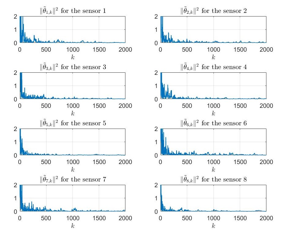
Figure 2: $\lVert\tilde{\theta}_{i,k}\rVert^{2}$ for each sensors.

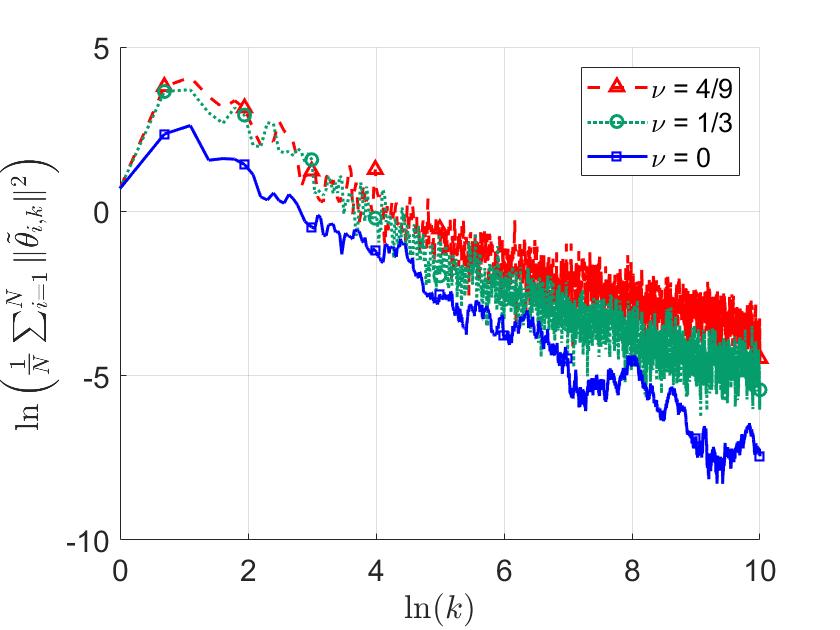
Figure 3: Convergence rates under different $\nu$.

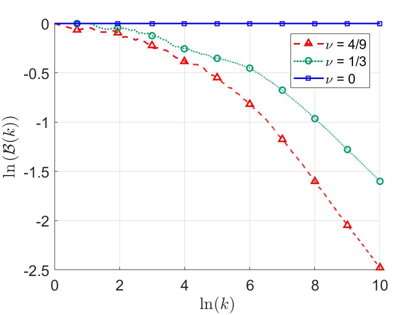
Figure 4: Average bit rates under different $\nu$.

8 Conclusion

This paper considers the distributed estimation under low communication cost, which is described by the average bit rates. A novel distributed estimation algorithm is proposed. In the algorithm, the SC consensus protocol [13] is used to fuse neighborhood information. A new stochastic event-triggered mechanism is designed to reduce the communication frequency. The algorithm has advantages both in the effectiveness and communication cost. For the effectiveness, the estimates of the algorithm are proved to converge to the true value in the almost sure and mean square sense. A polynomial almost sure convergence rate is also obtained. For the communication cost, the local and global average bit rates for communications are proved to decay to zero at polynomial rates. Besides, the trade-off between convergence rate and communication cost is established through event-triggered coefficients. A better convergence rate can be achieved by decreasing event-triggered coefficients, while lower communication cost can be achieved by increasing event-triggered coefficients.

There are interesting issues for future works. For example, how to extend the results to the cases with more complex communication graphs, such as directed graphs and switching graphs? Besides, Gan and Liu [8] consider the distributed order estimation, and Xie and Guo [32] investigate distributed adaptive filtering. These issues also suffer the communication cost problems. Then, how to apply our technique to these works to save the communication cost?

Appendix A Lemmas

Lemma A.1.

Let $f(\cdot)$ be the density function of $Lap(0,1)$. Given $C_{k}=\nu b\ln k$ with $\nu\geq 0$ and $b>0$, and a compact set $\mathcal{X}$, we have $\inf_{x\in\mathcal{X},k\in\mathbb{N}}\frac{k^{\nu}}{b}f((x-C_{k})/b)>0$.

Proof A.2.

If $\nu=0$, then $C_{k}=0$ for all $k$. Therefore, $\inf_{x\in\mathcal{X},k\in\mathbb{N}}\frac{1}{b}f(x/b)>0$ by the compactness of $\mathcal{X}$.

If $\nu>0$, then $\lim_{k\to\infty}C_{k}=\infty$, which together with the compactness of $\mathcal{X}$ implies that there exists $k_{0}$ such that $x-C_{k}<0$ for all $x\in\mathcal{X}$ and $k\geq k_{0}$. Hence,

$$\inf_{x\in\mathcal{X},k\geq k_{0}}\frac{k^{\nu}}{b}f\left(\frac{x-C_{k}}{b}\right)=\inf_{x\in\mathcal{X},k\geq k_{0}}\frac{k^{\nu}}{2b}e^{(x-\nu b\ln k)/b}=\frac{1}{2b}e^{\min\mathcal{X}/b}>0.$$

Besides by the compactness of $\mathcal{X}$, one can get $\inf_{x\in\mathcal{X}}\frac{k^{\nu}}{b}f((x-C_{k})/b)>0$ for all $k<k_{0}$. The lemma is proved.

Lemma A.3.

If positive sequence $\{z_{k}\}$ satisfies $\sum_{k=1}^{\infty}z_{k}=\infty$ and $z_{k+1}=O(z_{k})$, then for any $l\in\{1,\ldots,n\}$, $\sum_{q=1}^{\infty}\min_{n(q-1)+l<t\leq nq+l}z_{t}=\infty$.

Proof A.4.

Set $\bar{z}=\sup\left\{1,\frac{z_{k}+1}{z_{k}},k\in\mathbb{N}\right\}<\infty$. Then, $z_{k}\geq\frac{z_{k+1}}{\bar{z}}$. Therefore,

$$\sum_{q=1}^{\infty}\min_{n(q-1)+l<t\leq nq+l}z_{t}\geq\sum_{q=1}^{\infty}\max_{nq+l<t\leq n(q+1)+l}\frac{z_{t}}{\bar{z}^{2n}}\geq\frac{1}{n\bar{z}^{2n}}\sum_{k=l+n+1}^{\infty}z_{k}=\infty.$$

Lemma A.5.

Assume that

1. $\{\mathcal{F}_{k}\}$ is a $\sigma$-algebra sequence satisfying $\mathcal{F}_{k-1}\subseteq\mathcal{F}_{k}$ for all $k$;

2. $\{W_{k},\mathcal{F}_{k}\}$ is a martingale difference sequence satisfying $\mathbb{E}\left[\lVert W_{k}\rVert^{\rho}\middle|\mathcal{F}_{k-1}\right]=O\left(\frac{1}{k^{\rho b}}\right)$ almost surely for some $\rho>4$ and $b>\frac{1}{2}$;

3. $\{U_{k}\}$ is a positive definite matrix sequence. $U_{k}$ is $\mathcal{F}_{k-1}$-measurable. $U_{k}=O\left(k^{\mu}\right)$ for some $0\leq\mu<\frac{1}{2}$ almost surely. And,

   (29) $$\frac{1}{p}\sum_{t=k-p+1}^{k}U_{t}\geq aI_{n}$$

   for some $p\in\mathbb{N}$, $a>0$ and all $k\in\mathbb{N}$ almost surely;

4. $\{X_{k},\mathcal{F}_{k}\}$ is a sequence of adaptive random variables;

5. There exists $c>1$ almost surely such that

   (30) $$X_{k}=\left(I_{n}-\frac{U_{k}}{k}+O\left(\frac{1}{k^{c}}\right)\right)X_{k-1}+W_{k}.$$

Then,

$$X_{k}=\begin{cases}O\left(\frac{1}{k^{a}}\right),&\text{if}\ 2b^{\prime}-2a>1;\\ O\left(\frac{\ln k}{k^{b^{\prime}-1/2}}\right),&\text{if}\ 2b^{\prime}-2a=1;\\ O\left(\frac{\sqrt{\ln k}}{k^{b^{\prime}-1/2}}\right),&\text{if}\ 2b^{\prime}-2a<1,\end{cases}\ \text{a.s.},$$

where $b^{\prime}\leq\min\{b,1,\frac{3+2b-2\mu}{4}\}$.

Proof A.6.

By (30),

$$\mathbb{E}\left[\left\|X_{k}\right\|^{2}\middle|\mathcal{F}_{k-1}\right]$$

$$= \left(1+O\left(\frac{1}{k^{\min\{c,2-2\mu\}}}\right)\right)\left\|X_{k-1}\right\|^{2}-\frac{2}{k}X_{k-1}^{\top}U_{k}X_{k-1}+O\left(\frac{1}{k^{2b}}\right),\ \text{a.s.}$$

Then by Theorem 1 of [20], we have $\left\|X_{k}\right\|^{2}$ converges to a finite value almost surely, which implies the almost sure boundedness of $X_{k}$.

We estimate the almost sure convergence rate of $X_{k}$ in the following two cases.

Case 1: $2b^{\prime}-2a>1$. In this case, we have

(31) $$\mathbb{E}\left[(k+1)^{2a}\left\|X_{k}\right\|^{2}\middle|\mathcal{F}_{k-1}\right]$$

$$\leq\ \ \ \ \ \ \!\!\!\!\!\!\!\!\!\!\!\!\!\left(1+\frac{2a}{k}+O\left(\frac{1}{k^{\min\{c,2-2\mu\}}}\right)\right)k^{2a}\left\|X_{k-1}\right\|^{2}-\frac{2}{k^{1-2a}}X_{k-1}^{\top}U_{k}X_{k-1}+O\left(\frac{1}{k^{2b-2a}}\right)$$

$$=\ \ \ \ \ \ \!\!\!\!\!\!\!\!\!\!\!\!\!\left(1+O\left(\frac{1}{k^{\min\{c,2-2\mu\}}}\right)\right)k^{2a}\left\|X_{k-1}\right\|^{2}+\frac{2a}{k^{1-2a}}\left\|X_{k-1}\right\|^{2}-\frac{2}{k^{1-2a}}X_{k-1}^{\top}U_{k}X_{k-1}$$

$$\!\!\!\!\!\!\!\!\!\!\!\!\!+O\left(\frac{1}{k^{2b-2a}}\right),\ \text{a.s.}$$

We now prove that $\sup_{k\in\mathbb{N}}\sum_{t=1}^{k}\left(\frac{2a}{t^{1-2a}}\left\|X_{t-1}\right\|^{2}-\frac{2}{t^{1-2a}}X_{t-1}^{\top}U_{t}X_{t-1}\right)<\infty$ almost surely. Note that $1-2a>2-2b^{\prime}\geq 0$. Then by (29), one can get

(32) $$\!\!\!\!\!\!\!\!\sum_{t=1}^{k}\left(\frac{2a}{t^{1-2a}}\left\|X_{t-1}\right\|^{2}-\frac{2}{t^{1-2a}}X_{t-1}^{\top}U_{t}X_{t-1}\right)$$

$$\leq\sum_{r=0}^{\lfloor\frac{k}{p}\rfloor-1} \sum_{t=pr+1}^{pr+p}\left(\frac{2a}{t^{1-2a}}\left\|X_{t-1}\right\|^{2}-\frac{2}{t^{1-2a}}X_{t-1}^{\top}U_{t}X_{t-1}\right)+O\left(\frac{1}{k^{1-2a}}\right)$$

$$\leq\sum_{r=0}^{\lfloor\frac{k}{p}\rfloor-1} \!\!\frac{2}{(pr+p)^{1-2a}}\!\sum_{t=pr+1}^{pr+p}\!\!\left(a\left\|X_{t-1}\right\|^{2}-X_{t-1}^{\top}U_{t}X_{t-1}\right)+\!\!\sum_{r=0}^{\lfloor\frac{k}{p}\rfloor-1}\!\!O\left(\frac{1}{r^{2-2a}}\right)+O\left(1\right)$$

$$\leq\sum_{r=0}^{\lfloor\frac{k}{p}\rfloor-1} \frac{2}{(pr+p)^{1-2a}}\sum_{t=pr+1}^{pr+p}\left(X_{pr+p-1}^{\top}U_{t}X_{pr+p-1}-X_{t-1}^{\top}U_{t}X_{t-1}\right)$$

$$+\sum_{r=0}^{\lfloor\frac{k}{p}\rfloor-1}\!\!\!\!\!\! \ \ \ \ \frac{2a}{(pr+p)^{1-2a}}\sum_{t=pr+1}^{pr+p}\left(\left\|X_{t-1}\right\|^{2}-\left\|X_{pr+p-1}\right\|^{2}\right)+O\left(1\right).$$

Besides,

(33) $$\!\!\!\!\!\sum_{t=pr+1}^{pr+p}\left(X_{pr+p-1}^{\top}U_{t}X_{pr+p-1}-X_{t-1}^{\top}U_{t}X_{t-1}\right)$$

$$=\ \ \ \ \ \ \ \ \!\!\!\!\!\!\!\!\!\!\!\!\!\!\!\!\!\sum_{t=pr+1}^{pr+p}\sum_{l=t}^{pr+p-1}\left(X_{l}^{\top}U_{t}X_{l}-X_{l-1}^{\top}U_{t}X_{l-1}\right)$$

$$=\ \ \ \ \ \ \ \ \!\!\!\!\!\!\!\!\!\!\!\!\!\!\!\!\!\sum_{t=pr+1}^{pr+p}\sum_{l=t}^{pr+p-1}\left(2W_{l}^{\top}U_{t}\left(I_{n}-\frac{U_{l}}{l}+O\left(\frac{1}{l^{c}}\right)\right)X_{l-1}+W_{l}^{\top}U_{t}W_{l}\right)+O\left(r^{2\mu-1}\right),\ \text{a.s.}$$

When $t\in\left\{pq+1,\ldots,pq+l\right\}$ and $l=\{t,\ldots,pr+p-1\}$, it holds that

$$\frac{4}{(pr+p)^{1-2a}l^{b}}U_{t}\left(I_{n}-\frac{U_{l}}{l}+O\left(\frac{1}{l^{c}}\right)\right)X_{l-1}=O\left(\frac{1}{r^{1+b-2a-\mu}}\right).$$

Note that $1+b-2a-\mu>2+b-2b^{\prime}-\mu\geq\frac{1}{2}$. Then by Lemma 2 of [29], one can get

(34) $$\sum_{r=0}^{\lfloor\frac{k}{p}\rfloor-1}\!\!\sum_{t=pr+1}^{pr+p}\!\!\sum_{l=t}^{pr+p-1}\!\!(l^{b}W_{l})^{\top}\!\left(\frac{4}{(pr+p)^{1-2a}l^{b}}U_{t}\!\left(\!I_{n}-\frac{U_{l}}{l}+O\left(\frac{1}{l^{c}}\right)\!\right)\!X_{l-1}\!\right)\!\!=O(1),\ \text{a.s.}$$

In addition, by $1+2b-2a-\mu>1+b-2a-\mu>\frac{1}{2}$ and Lemma 2 of [29],

$$\sum_{r=0}^{\lfloor\frac{k}{p}\rfloor-1}\sum_{t=pr+1}^{pr+p}\frac{2}{(pr+p)^{1-2a}}\sum_{l=t}^{pr+p-1}W_{l}^{\top}U_{t}W_{l}$$

$$= \sum_{r=0}^{\lfloor\frac{k}{p}\rfloor-1}\sum_{t=pr+1}^{pr+p}\sum_{l=t}^{pr+p-1}\frac{2}{(pr+p)^{1-2a}t^{2b-\mu}}\cdot t^{2b-\mu}\left(W_{l}^{\top}U_{t}W_{l}-\mathbb{E}\left[W_{l}^{\top}U_{t}W_{l}\middle|\mathcal{F}_{l-1}\right]\right)$$

$$+\sum_{r=0}^{\lfloor\frac{k}{p}\rfloor-1}\sum_{t=pr+1}^{pr+p}\frac{2}{(pr+p)^{1-2a}}\sum_{l=t}^{pr+p-1}\mathbb{E}\left[W_{l}^{\top}U_{t}W_{l}\middle|\mathcal{F}_{l-1}\right]$$

$$= O(1)+\sum_{r=0}^{\lfloor\frac{k}{p}\rfloor-1}\sum_{t=pr+1}^{pr+p}O\left(\frac{1}{r^{2a+\mu-2b-1}}\right)=O(1),\ \text{a.s.},$$

which together with (33) and (34) implies that

$$\sum_{r=0}^{\lfloor\frac{k}{p}\rfloor-1}\frac{2}{(pr+p)^{1-2a}}\sum_{t=pr+1}^{pr+p}\left(X_{pr+p-1}^{\top}U_{t}X_{pr+p-1}-X_{t-1}^{\top}U_{t}X_{t-1}\right)=O(1),\ \text{a.s.}$$

Similarly, one can get

$$\sum_{r=0}^{\lfloor\frac{k}{p}\rfloor-1}\frac{2a}{(pr+p)^{1-2a}}\sum_{t=pr+1}^{pr+p}\left(\left\|X_{t-1}\right\|^{2}-\left\|X_{pr+p-1}\right\|^{2}\right)=O(1),\ \text{a.s.}$$

Then by (32), we have

(35) $$\sum_{t=1}^{k}\left(\frac{2a}{t^{1-2a}}\left\|X_{t-1}\right\|^{2}-\frac{2}{t^{1-2a}}X_{t-1}^{\top}U_{t}X_{t-1}\right)<\infty,\ \text{a.s.},$$

Given $S_{0}>0$, define $S_{k}=S_{0}-\sum_{t=1}^{k}\left(\frac{2a}{t^{1-2a}}\left\|X_{t-1}\right\|^{2}-\frac{2}{t^{1-2a}}X_{t-1}^{\top}U_{t}X_{t-1}\right)$ and $V_{k}=(k+1)^{2a}\left\|X_{k}\right\|^{2}+S_{k}$. Hence by (31), we have

$$\mathbb{E}\left[V_{k}\middle|\mathcal{F}_{k-1}\right]\leq\left(1+O\left(\frac{1}{k^{\min\{c,2-2\mu\}}}\right)\right)V_{k-1}+O\left(\frac{1}{k^{2b-2a}}\right),\ \text{a.s.}$$

Then define $k_{0}=\inf\{k:S_{k}<0\}$. We have

$$\mathbb{E}\left[V_{\min\{k,k_{0}\}}\middle|\mathcal{F}_{k-1}\right]$$

$$\leq V_{k_{0}}I_{\{k_{0}\leq k\}}+\left(1+O\left(\frac{1}{k^{\min\{c,2-2\mu\}}}\right)\right)V_{k-1}I_{\{k_{0}>k\}}+O\left(\frac{1}{k^{2b-2a}}\right)$$

$$\leq \left(1+O\left(\frac{1}{k^{\min\{c,2-2\mu\}}}\right)\right)V_{\min\{k-1,k_{0}\}}+O\left(\frac{1}{k^{2b-2a}}\right).$$

By Theorem 1 of [20], $V_{\min\{k,k_{0}\}}$ converges to a finite value almost surely. Note that $V_{k}=V_{\min\{k,k_{0}\}}$ in the set

$$\{k_{0}=\infty\}=\{\inf_{k}S_{k}\geq 0\}=\left\{\sum_{t=1}^{k}\left(\frac{2a}{t^{1-2a}}\left\|X_{t-1}\right\|^{2}-\frac{2}{t^{1-2a}}X_{t-1}^{\top}U_{t}X_{t-1}\right)<S_{0}\right\}.$$

Then by the arbitrariness of $S_{0}$ and (35), $V_{k}$ converges to a finite value almost surely, which implies the almost sure boundedness of $(k+1)^{2a}\left\|X_{k}\right\|^{2}$. Hence, one can get $X_{k}=O\left(\frac{1}{k^{a}}\right)$ almost surely.

Case 2: $2b^{\prime}-2a\leq 1$. In this case, we have

(36) $$\mathbb{E}\left[\frac{(k+1)^{2b^{\prime}-1}}{(\ln(k+1))^{2}}\left\|X_{k}\right\|^{2}\middle|\mathcal{F}_{k-1}\right]$$

$$\leq \left(1+\frac{2b^{\prime}-1}{k}+O\left(\frac{1}{k^{\min\{c,2-2\mu\}}}\right)\right)\frac{k^{2b^{\prime}-1}}{(\ln k)^{2}}\left\|X_{k-1}\right\|^{2}$$

$$-\frac{2}{k^{2-2b}(\ln k)^{2}}X_{k-1}^{\top}U_{k}X_{k-1}+O\left(\frac{1}{k(\ln k)^{2}}\right)$$

$$\leq \left(1+O\left(\frac{1}{k^{\min\{c,2-2\mu\}}}\right)\right)\frac{k^{2b^{\prime}-1}}{(\ln k)^{2}}\left\|X_{k-1}\right\|^{2}+\frac{2a}{k^{2-2b^{\prime}}(\ln k)^{2}}\left\|X_{k-1}\right\|^{2}$$

$$-\frac{2}{k^{2-2b^{\prime}}(\ln k)^{2}}X_{k-1}^{\top}U_{k}X_{k-1}+O\left(\frac{1}{k(\ln k)^{2}}\right),\ \text{a.s.}$$

Then, similar to the case of $2b^{\prime}-2a>1$, we have $X_{k}=O\left(\frac{\ln k}{k^{b^{\prime}-1/2}}\right)$ almost surely.

We further promote the almost sure convergence rate for the case of $2b^{\prime}-2a<1$. Since $X_{k}=O\left(\frac{\ln k}{k^{b^{\prime}-1/2}}\right)$ almost surely, one can get

(37) $$\!\!(k+1)^{2b^{\prime}-1}\left\|X_{k}\right\|^{2}$$

$$\leq\ \ \ \ \ \ \ \ \!\!\!\!\!\!\!\!\!\!\!\!\!\!\!k^{2b^{\prime}-1}\left\|X_{k-1}\right\|^{2}+2(k+1)^{2b^{\prime}-1}W_{k}^{\top}\left(\!I_{n}-\frac{U_{k}}{k}+O\left(\frac{1}{k^{c}}\right)\!\right)X_{k-1}+\frac{2b^{\prime}-1}{k^{2-2b^{\prime}}}\left\|X_{k-1}\right\|^{2}$$

$$\!\!\!\!\!\!\!\!\!\!\!\!\!\!\!-\frac{2}{k^{2-2b^{\prime}}}X_{k-1}^{\top}U_{k}X_{k-1}+(k+1)^{2b^{\prime}-1}\left(W_{k}^{2}-\mathbb{E}\left[W_{k}^{2}\middle|\mathcal{F}_{k-1}\right]\right)+O\left(\frac{1}{k}\right).$$

By Lemma 2 of [29], it holds that

$$\sum_{t=1}^{k}2(t+1)^{2b^{\prime}-1}W_{t}^{\top}\left(I_{n}-\frac{U_{t}}{t}+O\left(\frac{1}{t^{c}}\right)\right)X_{t-1}$$

$$= \sum_{t=1}^{k}((t+1)^{b}W_{t})^{\top}\left(2(t+1)^{2b^{\prime}-b-1}\left(I_{n}-\frac{U_{t}}{t}+O\left(\frac{1}{t^{c}}\right)\right)X_{t-1}\right)$$

$$= O(1)+o\left(\sum_{t=1}^{k}\frac{1}{t^{2-2b^{\prime}}}\lVert X_{t}\rVert^{2}\right),\ \text{a.s.},$$

and

$$\sum_{t=1}^{k}(t+1)^{2b^{\prime}-1}\left(W_{t}^{2}-\mathbb{E}\left[W_{t}^{2}\middle|\mathcal{F}_{k-1}\right]\right)$$

$$= \sum_{t=1}^{k}(t+1)^{2b}\left(W_{t}^{2}-\mathbb{E}\left[W_{t}^{2}\middle|\mathcal{F}_{k-1}\right]\right)\cdot\frac{1}{(t+1)^{1+2b^{\prime}-2b}}=O(1),\ \text{a.s.}$$

Similar to (35), we have

$$\sum_{t=1}^{k}\left(\frac{2a}{t^{2-2b^{\prime}}}\left\|X_{t-1}\right\|^{2}-\frac{2}{t^{2-2b^{\prime}}}X_{t-1}^{\top}U_{t}X_{t-1}\right)=o(\ln k),\ \text{a.s.}$$

Hence by (37),

$$(k+1)^{2b^{\prime}-1}\left\|X_{k}\right\|^{2}$$

$$\leq \left\|X_{0}\right\|^{2}+\sum_{t=1}^{k}2(t+1)^{2b^{\prime}-1}W_{t}^{\top}\left(I_{n}-\frac{U_{t}}{t}+O\left(\frac{1}{t^{c}}\right)\right)X_{t-1}$$

$$-\sum_{t=1}^{k}\frac{1+2a-2b^{\prime}}{t^{2-2b^{\prime}}}\left\|X_{t-1}\right\|^{2}+\sum_{t=1}^{k}\left(\frac{2a}{t^{2-2b^{\prime}}}\left\|X_{t-1}\right\|^{2}-\frac{2}{t^{2-2b^{\prime}}}X_{t-1}^{\top}U_{t}X_{t-1}\right)$$

$$+\sum_{t=1}^{k}(t+1)^{2b^{\prime}-1}\left(W_{t}^{2}-\mathbb{E}\left[W_{t}^{2}\middle|\mathcal{F}_{k-1}\right]\right)+O(\ln k)$$

$$\leq o\left(\sum_{t=1}^{k}\frac{1}{t^{2-2b^{\prime}}}\left\|X_{t}\right\|^{2}\right)-\left(1+2a-2b^{\prime}\right)\sum_{t=1}^{k}\frac{1}{t^{2-2b^{\prime}}}\left\|X_{t}\right\|^{2}+O(\ln k)=O(\ln k),\ \text{a.s.},$$

which implies $X_{k}=O\left(\frac{\sqrt{\ln k}}{k^{b^{\prime}-1/2}}\right)$. The lemma is thereby proved.

References

- [1] D. Alistarh, D. Grubic, J. Li, R. Tomioka, and M. Vojnovic, QSGD: Communication-efficient SGD via gradient quantization and encoding, in Proceedings of Advances in Neural Information Processing Systems, Long Beach, CA, 2017.
- [2] T. C. Aysal, M. J. Coates, and M. G. Rabbat, Distributed average consensus with dithered quantization, IEEE Trans. Signal Process., 56 (2008), pp. 4905–4918.
- [3] R. Carli and F. Bullo, Quantized coordination algorithms for rendezvous and deployment, SIAM J. Control Optim., 48 (2009), pp. 1251–1274.
- [4] R. Carli, F. Fagnani, A. Speranzon, and S. Zampieri, Communication constraints in the average consensus problem, Automatica, 44 (2008), pp. 671–684.
- [5] M. Carpentiero, V. Matta, and A. H. Sayed, Distributed Adaptive Learning Under Communication Constraints, IEEE Open Journal of Signal Processing, (2023), https://doi.org/10.1109/OJSP.2023.3344052.
- [6] Z. Chang, W. Song, J. Wang, and Z. Li, Fully distributed event-triggered affine formation maneuver control over directed graphs, Sci. China Inf. Sci., 66 (2023), pp. 1–3.
- [7] G. Chen, D. Yao, Q. Zhou, H. Li, and R. Lu, Distributed event-triggered formation control of USVs with prescribed performance, J. Syst. Sci. Complex., 35 (2022), pp. 820–838.
- [8] D. Gan and Z. Liu, Distributed order estimation of ARX model under cooperative excitation condition, SIAM J. Control Optim., 60 (2022), pp. 1519–1545.
- [9] X. He, Y. Xing, J. Wu, and K. H. Johansson, Event-triggered distributed estimation with decaying communication rate, SIAM J. Control Optim., 60 (2022), pp. 992–1017.
- [10] S. Kar, G. Hug, J. Mohammadi, and J. M. Moura, Distributed state estimation and energy management in smart grids: A consensusinnovations approach, IEEE J. Sel. Top. Signal Process., 8 (2014), pp. 1022–1038.
- [11] S. Kar, J. M. Moura, and H. V. Poor, Distributed linear parameter estimation: Asymptotically efficient adaptive strategies, SIAM J. Control Optim., 51 (2013), pp. 2200–2229.
- [12] S. Kar, J. M. Moura, and K. Ramanan, Distributed parameter estimation in sensor networks: Nonlinear observation models and imperfect communication, IEEE Trans. Inform. Theory, 58 (2012), pp. 3575–3605.
- [13] J. M. Ke, Y. L. Zhao, and J. F. Zhang, Signal comparison average consensus algorithm under binary-valued communications, in Proceedings of the IEEE Conference on Decision and Control, Singapore, 2023.
- [14] X. Lao, W. Du, and C. Li, Quantized distributed estimation with adaptive combiner, IEEE Trans. Signal Inf. Process. Netw., 8 (2022), pp. 187–200.
- [15] J. Li and G. AlRegib, Distributed estimation in energy-constrained wireless sensor networks, IEEE Trans. Signal Process., 57 (2009), pp. 3746–3758.
- [16] T. Li, M. Fu, L. Xie, and J. F. Zhang, Distributed consensus with limited communication data rate, IEEE Trans. Automat. Control, 56 (2011), pp. 279–292.
- [17] S. Liu, T. Li, and L. Xie, Distributed consensus for multiagent systems with communication delays and limited data rate, SIAM J. Control Optim., 49 (2011), pp. 2239–2262.
- [18] D. Jakovetic, M. Vukovic, D. Bajovic, A. K. Sahu, and S. Kar, Distributed recursive estimation under heavy-tail communication noise, SIAM J. Control Optim., 61 (2023), pp. 1582-1609.
- [19] Y. Meng, T. Li, and J. F. Zhang, Finite-level quantized synchronization of discrete-time linear multiagent systems with switching topologies, SIAM J. Control Optim., 55 (2017), pp. 275–299.
- [20] H. Robbins and D. Siegmund, A convergence theorem for non negative almost supermartingales and some applications, in Optimizing Methods in Statistics, Academic Press, New York, 1971, pp. 233–257.
- [21] A. K. Sahu, D. Jakovetić, and S. Kar, : A distributed random fields estimator, IEEE Trans. Signal Process., 66 (2018), pp. 4980–4995.
- [22] A. H. Sayed, Diffusion adaptation over networks, in Academic Press Library in Signal Processing, R. Chellapa and S. Theodoridis, eds., 2014, pp. 323–454.
- [23] M. O. Sayin and S. S. Kozat, Compressive diffusion strategies over distributed networks for reduced communication load, IEEE Trans. Signal Process., 62 (2014), pp. 5308–5323.
- [24] A. N. Shiryaev, Probability, 2nd ed., Springer, New York, 1996.
- [25] J. Wang, T. Li, and X. Zhang, Decentralized cooperative online estimation with random observation matrices, communication graphs and time delays, IEEE Trans. Inform. Theory, 67 (2021), pp. 4035–4059.
- [26] J. M. Wang, J. W. Tan, and J. F. Zhang, Differentially private distributed parameter estimation, J. Syst. Sci. Complex., 36 (2023), pp. 187–204.
- [27] T. Wang, H. Zhang, and Y. L. Zhao, Consensus of multi-agent systems under binary-valued measurements and recursive projection algorithm, IEEE Trans. Automat. Control, 65 (2019), pp. 2678–2685.
- [28] Z. Wang, C. Jin, W. He, M. Xiao, G. P. Jiang, and J. D. Cao, Event-triggered impulsive synchronization of heterogeneous neural networks, Sci. China Inf. Sci., (2023), https://doi.org/10.1007/s11432-022-3839-y.
- [29] C. Z. Wei, Asymptotic properties of least-squares estimates in stochastic regression models, Ann. Statist., 13 (1985), pp. 1498–1508.
- [30] X. Wu, B. Mao, X. Wu, and J. Lü, Dynamic event-triggered leader-follower consensus control for multiagent systems, SIAM J. Control Optim., 60 (2022), pp. 189–209.
- [31] S. L. Xie and H. R. Li, Distributed LMS estimation over networks with quantised communications, Internat. J. Control, 86 (2013), pp. 478–492.
- [32] S. Xie and L. Guo, Analysis of normalized least mean squares-based consensus adaptive filters under a general information condition, SIAM J. Control Optim., 56 (2018), pp. 3404–3431.
- [33] Q. Zhang and J. F. Zhang, Distributed parameter estimation over unreliable networks with Markovian switching topologies, IEEE Trans. Automat. Control, 57 (2012), pp. 2545-2560.
- [34] Y. L. Zhao, T. Wang, and W. Bi, Consensus protocol for multiagent systems with undirected topologies and binary-valued communications, IEEE Trans. Automat. Control, 64 (2019), pp. 206–221.
- [35] S. Zhu, C. Chen, J. Xu, X. Guan, L. Xie, and K. H. Johansson, Mitigating quantization effects on distributed sensor fusion: A least squares approach, IEEE Trans. Signal Process., 66 (2018), pp. 3459–3474.
- [36] S. Zhu, Y. C. Soh, and L. Xie, Distributed parameter estimation with quantized communication via running average, IEEE Trans. Signal Process., 63 (2015), pp. 4634–4646.
- [37] V. A. Zorich, Mathematical Analysis I, 2nd ed., Springer, New York, 2015.