Movable Antenna Empowered Downlink NOMA Systems: Power Allocation and Antenna Position Optimization

Abstract

This paper investigates a novel communication paradigm employing movable antennas (MAs) within a multiple-input single-output (MISO) non-orthogonal multiple access (NOMA) downlink framework, where users are equipped with MAs. Initially, leveraging the far-field response, we delineate the channel characteristics concerning both the power allocation coefficient and positions of MAs. Subsequently, we endeavor to maximize the channel capacity by jointly optimizing power allocation and antenna positions. To tackle the resultant non-concave problem, we propose an alternating optimization (AO) scheme underpinned by successive convex approximation (SCA) to converge towards to a stationary point. Through numerical simulations, our findings substantiate the superiority of the MA-assisted NOMA system over both orthogonal multiple access (OMA) and conventional NOMA configurations in terms of average sum rate and outage probability.

I Introduction

In light of the worldwide proliferation of fifth-generation (5G) wireless services and applications, scholars are intensifying their focus on the investigation of sixth-generation (6G) wireless communication to achieve augmented available bandwidth, heightened spectrum efficiency, and diminished outage probability [1, 2]. Multiple-input multiple-output (MIMO) stands as a cornerstone technology in the 6G wireless standard, enhancing the efficiency of wireless communication through the exploitation of innovative degrees of freedom (DoFs) within the spatial domain. Numerous researchers leverage MIMO technology, integrating it with other promising techniques, yielding notable outcomes [3, 4, 5]. Nevertheless, the antenna arrangement in conventional MIMO systems remains fixed, lacking adaptability to accommodate abrupt channel fading.

In response to the limitations inherent in conventional antenna configurations, a pioneering antenna arrangement, namely the movable antenna (MA) was introduced in [6]. This innovative design permits the antenna to maneuver within a two-dimensional (2D) region, thereby tacking sudden channel fading by dynamically adjusting the signal phases across various propagation paths upon reaching the receivers. In systems employing MAs, each antenna is interconnected with the radio frequency (RF) chain via a flexible cable, thereby enabling adjustments in its physical positions through the utilization of electromechanical devices, such as step motors [7]. The mobility endowed to these antennas facilitates the dynamic modification of the channel response, tantamount to the real-time reconfiguration of the optimal channel between the base station (BS) and users, thereby significantly enhancing the performance of communication systems [8]. In [9], researchers investigated a multi-user downlink communication system featuring a BS equipped with fixed position antennas (FPAs) and users possessing a single MA. It is illustrated that this configuration could achieve lower power consumption under equivalent outage probability conditions through the joint optimization of beam-forming at the BS and antenna positions adjusting at the users. The authors in [10] considered a multi-user downlink system wherein the BS is outfitted with MAs, while the users possess a single FPA.

On the other hand, none-orthogonal multiple access (NOMA) stands as a pivotal multiple access technique in bolstering the forthcoming Internet-of-Things (IoTs) and mobile internet landscapes [11, 12, 13]. The fundamental premise of NOMA resides in enabling disparate users to share the same communication resource (i.e., time, frequency, code), while distinguishing their respective signals through varying power allocation. Accurate decoding for users is guaranteed through the employment of superposition coding (SC) at the transmitter and successive interference cancellation (SIC) at the receiver. Researchers demonstrated that systems employing NOMA can attain superior spectrum and power efficiency than that of adopting conventional orthogonal multiple access (OMA) as indicated in [14, 15]. Nonetheless, a notable phenomenon arises wherein users employing NOMA are more susceptible to experiencing outage events when encountering inferior channel conditions.

Inspired by the aforementioned description, we consider the integration of NOMA and MA, which can enhance the efficiency of multiple access for MA users and improve the communication reliability for NOMA users. We investigate the MA-assisted NOMA downlink communication system, and then we formulate the problem of maximizing the channel capacity by joint optimization of power allocation and antenna positions. Given the inherent non-concave nature of this problem, rendering it challenging to solve directly, we propose an alternating optimization (AO) algorithm capitalizing on successive convex approximation (SCA) to iteratively converge towards a stationary point.

II System Model and Problem Formulation

As depicted in Fig. 1, we consider a multiple-input single-output (MISO) downlink communication architecture incorporating NOMA and MA technologies. Within this framework, a BS featuring a constellation of $N$ FPAs caters to two distinct users each equipped with a single MA. We designate the first user, termed as the user1, as proximal to the BS relative to the second user, denoted as the user2.

Through the implementation of power-domain NOMA, the transmitted signal from each antenna at the BS is presumed to be uniform and can be mathematically expressed as follows

$$s=\sqrt{\alpha}\cdot{s_{1}}+\sqrt{1-\alpha}\cdot{s_{2}},$$ (1)

where $\alpha$ represents the allocation coefficient of transmitting power for user1, whereas $1-\alpha$ represents that for user2; $s_{1},s_{2}\in\mathbb{C}^{1\times 1}$ denote signals sent to user1 and user2 respectively with normalized power, which are mutually independent, i.e., $\mathbb{E}(s^{*}s)=1$.

Suppose the total transmitting power of the BS is denoted as $P$, where each antenna possesses an equal power represented as $P_{0}=\frac{P}{N}$. The position of the $k$-th antenna at BS can be described as $\mathbf{t}_{k}=\left[x^{t}_{k},y^{t}_{k}\right]^{T},1\leq k\leq N$, by establishing via 2D local coordinate system. Similarly, the position of the MA corresponding to the $i$-th user can be represented as $\mathbf{r}_{i}=\left[x^{r}_{i},y^{r}_{i}\right]^{T}\in\mathcal{D}_{i},i={1,2}$, where $\mathcal{D}_{i}$ is the 2D square region for MA of the $i$-th user moving with the identical size of $A\times A$. Then, throughout the downlink communication procedure, the received baseband signal of the $i$-th user can be expressed as follows

$$y_{i}=h_{i}(\mathbf{r}_{i})\cdot P_{0}\cdot s+n_{i},$$ (2)

where $h_{i}(\mathbf{r_{i}})\in\mathbb{C}^{1\times 1}$ is the channel response coefficient (CRC) between the BS and user $i,i={1,2}$; $n_{i}\in\mathbb{C}^{1\times 1}$ represents the addictive white Gaussian noise (AWGN) in the received signal of user $i$ with the average noise power $\sigma^{2}$, i.e., $\mathbf{n}=\left[n_{1},n_{2}\right]^{T}\sim\mathcal{CN}\left(\mathbf{0},\sigma^{2}\mathbf{I_{2}}\right)$.

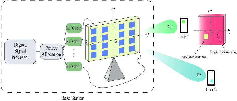
Figure 1: MA-assisted NOMA downlink communication system.

In this system, we focus on a field response channel[6]. The number of transmit paths from the BS origin $\mathbf{o}^{t}=[0,0]^{T}$ to the origin of the $i$-th user $\mathbf{o}^{r}_{i}=[0,0]^{T}$ is $L_{i}^{t}$; similarly, the number of receive paths is $L_{i}^{r}$. Therefore, the path response matrix (PRM) between the BS and the $i$-th user is defined as $\mathbf{\Sigma}_{i}\in\mathbb{C}^{L^{r}_{i}\times L^{t}_{i}}$, where $\mathbf{\Sigma}_{i}\left[n,m\right]$ represents the CRC between the $m$-th transmit path and the $n$-th receive path from the BS origin to that of the user $i$. According to the far field response model, the movements of MA are not anticipated to alter the angle-of-departure (AoD), the angle-of-arrival (AoA), or the amplitude of the CRC for each channel path extending from the BS to users. For the $i$-th user, the discrepancy in signal propagation for the $m$-th transmit path between the position of $k$-th antenna $\mathbf{t}_{k}=[x_{k},y_{k}]^{T}$ and original point $\mathbf{0}^{t}=[0,0]^{T}$ can be described as $\rho^{t}_{i,m}(\mathbf{t}_{k})=-[x_{k}^{t}\cos\theta^{t}_{i,m}\sin\phi^{t}_{i,m}+y_{k}^{t}\sin\theta^{t}_{i,m}]$, where $\theta^{t}_{i,m}$ and $\phi^{t}_{i,m}$ represent the elevation and azimuth of the AoD for the $m$-th transmit path to user $i$ respectively. Consequently, its associated phase shift is denoted as $-j\frac{2\pi}{\lambda}\cdot\rho^{t}_{i,m}(\mathbf{t}_{k})$, where $\lambda$ is the carrier wavelength. Subsequently, the transmit field response vector (FRV) of the $k$-th FPA at the BS can be derived as follows

$$\mathbf{g}_{i}(\mathbf{t}_{k})=[e^{-j\frac{2\pi}{\lambda}\rho^{t}_{i,1}(\mathbf{t}_{k})},e^{-j\frac{2\pi}{\lambda}\rho^{t}_{i,2}(\mathbf{t}_{k})},\cdots,e^{-j\frac{2\pi}{\lambda}\rho^{t}_{i,L_{i}^{t}}(\mathbf{t}_{k})}]^{T}.$$ (3)

Similarly, the receive FPV of the $i$-th user can be described as

$$\mathbf{f}_{i}(\mathbf{r}_{i})=[e^{-j\frac{2\pi}{\lambda}\rho^{r}_{i,1}(\mathbf{r}_{i})},e^{-j\frac{2\pi}{\lambda}\rho^{r}_{i,2}(\mathbf{r}_{i})},\cdots,e^{-j\frac{2\pi}{\lambda}\rho^{r}_{i,L_{i}^{r}}(\mathbf{r}_{i})}]^{T},$$ (4)

where $\rho^{r}_{i,n}(\mathbf{r}_{i})=x_{i}^{r}\cos\theta^{r}_{i,n}\sin\phi^{r}_{i,n}+y_{i}^{r}\sin\theta^{r}_{i,n}$ represents the signal propagation difference for $n$-th receive path between the position of MA $\mathbf{r}_{i}=[x_{i}^{r},y_{i}^{r}]^{T}$ and original point $\mathbf{o}_{i}^{r}=[0,0]^{T}$ at user $i$. And $\theta^{r}_{i,n},\phi^{r}_{i,n}$ denote the elevation and azimuth of the AoA for the $n$-th receive path to user $i$ separately. Thus, the CRC between the BS and user $i$ can be obtained as

$$h_{i}(\mathbf{r}_{i})=\mathbf{f}_{i}(\mathbf{r}_{i})^{T}\cdot\mathbf{\Sigma}_{i}\cdot\mathbf{G}_{i}\cdot\mathbf{1},$$ (5)

where $\mathbf{G}_{i}=[\mathbf{g}_{i}(\mathbf{t}_{1}),\mathbf{g}_{i}(\mathbf{t}_{2}),\cdots,\mathbf{g}_{i}(\mathbf{t}_{N})]\in\mathbb{C}^{L_{i}^{t}\times N},i={1,2}$ is the transmit field response matrix (FRM) from the BS to the $i$-th user; $\mathbf{1}=[1,1,\cdots,1]^{T}\in\mathbb{R}^{N\times 1}$ represents the all-one vector.

In adherence to the fundamental concept of SIC, the power allocation coefficient is lower for the user experiencing an robust channel condition, denoted as $\alpha_{s}\triangleq\min\{\alpha,1-\alpha\}$. Thus, the signal-to-noise-plus-interference ratio (SINR) for the user encountering a robust channel condition is denoted as $\gamma_{s}$, while that of the user suffering an inferior channel condition is given as $\gamma_{w}$, as exhibited bellow.

$$\gamma_{s} =\frac{P_{0}\cdot\alpha_{s}\cdot\max{\{\left|h_{1}(\mathbf{r}_{1})\right|^{2},\left|h_{2}(\mathbf{r}_{2})\right|^{2}\}}}{\sigma^{2}}$$ (6)

$$\gamma_{w} =\frac{P_{0}\cdot(1-\alpha_{s})\cdot\min{\{\left|h_{1}(\mathbf{r}_{1})\right|^{2},\left|h_{2}(\mathbf{r}_{2})\right|^{2}\}}}{P_{0}\cdot\alpha_{s}\cdot\min{\{\left|h_{1}(\mathbf{r}_{1})\right|^{2},\left|h_{2}(\mathbf{r}_{2})\right|^{2}\}}}$$ (7)

The primary objective of this study is to maximize channel capacity through the joint optimization of both the power allocation coefficient and the position of MA for each user. We posit that successful decoding of the transmitted signal by users occurs when SINR surpasses a predetermined threshold $\gamma_{0}$. Drawing on the Shannon capacity theorem, this optimization problem can be formulated as

(P $$\text{0)}\quad\max_{\{\alpha_{s},\mathbf{r}_{1},\mathbf{r}_{2}\}}\log_{2}\left(1+\gamma_{s}\right)+\log_{2}\left(1+\gamma_{w}\right),$$ (8a)

s. $$\text{t.}\qquad\qquad\qquad\qquad\gamma_{s}\geqslant\gamma_{0},$$ (8b)

$$\quad\quad\quad\quad\frac{\rho\cdot\left(1-\alpha_{s}\right)\cdot\left|h_{i}(\mathbf{r}_{i})\right|^{2}}{\rho\cdot\alpha_{s}\cdot\left|h_{i}(\mathbf{r}_{i})\right|^{2}+1}\geqslant\gamma_{0},\enspace i={1,2},$$ (8c)

$$\enspace\quad\quad\quad\quad\quad\quad\quad\enspace 0\leqslant\alpha_{s}\leqslant 1,$$ (8d)

$$\quad\quad\quad\quad\quad\quad\quad\quad\quad\mathbf{r}_{i}\in\mathcal{D}_{i},\quad\quad\quad\quad i={1,2},$$ (8e)

where $\rho=\frac{P_{0}}{\sigma^{2}}$ represents the ratio between the transmitting power of each antenna and the average noise power; constraints (8b), (8c) specify the minimal SINR necessary for accurate signal decoding by users; constraint (8e) mandates that the MAs of users remain within the designated square region. Due to the non-convex nature of the objective function and constraints (8b), (8c), the optimization problem is inherently non-concave, posing challenges for directly obtaining the optimal solution.

III Proposed Solution

In this section, we introduce an alternating optimization algorithm for addressing (P0), which involves decomposing it into two sub-problems, denoted as (P1) and (P2), respectively. The optimization process alternates between refining the power allocation coefficient and adjusting the positions of MAs while holding the other side constant. Initially, we fix the positions of MAs. Then, exploiting the monotonicity of the logarithmic function, we formulate sub-problem (P1) as follows

(P $$\text{1)}\quad\max_{\{\alpha_{s}\}}\quad\left(1+\gamma_{s}\right)\times\left(1+\gamma_{w}\right),$$ (9a)

s. $$\text{t.}\quad\quad\quad\quad\quad\text{(8b), (8c), (8d)},$$

The objective function of (P1) is denoted as $m(\alpha_{s})$, and we proceed to calculate its first derivative as follows

$$m^{{}^{\prime}}(\alpha_{s})=\tfrac{\rho\cdot(1+\rho\cdot\min{\{\left|h_{1}(\mathbf{r}_{1})\right|^{2},\left|h_{2}(\mathbf{r}_{2})\right|^{2}\}})\cdot\left|\left|h_{1}(\mathbf{r}_{1})\right|^{2}-\left|h_{2}(\mathbf{r}_{2})\right|^{2}\right|}{\left(\rho\cdot\alpha_{s}\cdot\min{\{\left|h_{1}(\mathbf{r}_{1})\right|^{2},\left|h_{2}(\mathbf{r}_{2})\right|^{2}\}}+1\right)^{2}}.$$ (10)

Additionally, under constraint (8b), we can obtain a lower bound for $\alpha_{s}$, and two separate upper bounds can be derived based on constraint (8c), as shown bellow.

$$\quad\alpha_{s} \geqslant\frac{\gamma_{0}}{\rho\cdot\max{\{\left|h_{1}(\mathbf{r}_{1})\right|^{2},\left|h_{2}(\mathbf{r}_{2})\right|^{2}\}}}\triangleq l_{1},$$ (11)

$$\alpha_{s} \leqslant\frac{\rho\cdot\max{\{\left|h_{1}(\mathbf{r}_{1})\right|^{2},\left|h_{2}(\mathbf{r}_{2})\right|^{2}\}}-\gamma_{0}}{\rho\cdot\max{\{\left|h_{1}(\mathbf{r}_{1})\right|^{2},\left|h_{2}(\mathbf{r}_{2})\right|^{2}\}}\cdot(1+\gamma_{0})}\triangleq\mu_{1},$$ (12)

$$\alpha_{s} \leqslant\frac{\rho\cdot\min{\{\left|h_{1}(\mathbf{r}_{1})\right|^{2},\left|h_{2}(\mathbf{r}_{2})\right|^{2}\}}-\gamma_{0}}{\rho\cdot\min{\{\left|h_{1}(\mathbf{r}_{1})\right|^{2},\left|h_{2}(\mathbf{r}_{2})\right|^{2}\}}\cdot(1+\gamma_{0})}\triangleq\mu_{2}.$$ (13)

Depending on the non-negativity of $m^{{}^{\prime}}(\alpha_{s})$ and the varied relationships between the lower bound and upper bounds for $\alpha_{s}$, the optimal solution for (P1) exhibits distinct cases as follows (The user encountering inferior channel conditions is denoted as WU, in contrast to the user experiencing robust channel conditions, designated as SU.).

Case I: $l_{1}\leqslant\mu_{2}\leqslant\mu_{1}$, a feasible optimal solution $\alpha_{s}^{\star}=\mu_{2}$ for (P1) exists. In cases where the aforementioned relationship cannot be precisely satisfied, an outage event occurs within the communication system.

Case II: $0\leqslant\mu_{2}<l_{1}\leqslant\mu_{1}$, in this scenario, there must be one user experiencing an outage event. The maximum data rate for the SU is denoted as $\log_{2}\left(1+\frac{\rho\cdot\max{\{\left|h_{1}(\mathbf{r}_{1})\right|^{2},\left|h_{2}(\mathbf{r}_{2})\right|^{2}\}}-\gamma_{0}}{1+\gamma_{0}}\right)\triangleq R_{1}$, while for the WU, it is $\log_{2}\left(1+\rho\cdot\min{\{\left|h_{1}(\mathbf{r}_{1})\right|^{2},\left|h_{2}(\mathbf{r}_{2})\right|^{2}\}}\right)\triangleq R_{2}$. The WU encounters an outage event to maximize channel capacity, when $R_{1}\geqslant R_{2}$; conversely, the SU experiences an outage event. And we rule that in the event of an outage, the data rate for the affected user is reduced to 0.

Case III: $\mu_{2}<0<l_{1}\leqslant\mu_{1}$, the constraint necessary for accurately decoding signals to the WU remains unsatisfied, resulting in a perpetual outage for the WU. And the optimal $\alpha_{s}$ which maximizes channel capacity, is denoted as $\alpha_{s}^{\star}=\mu_{1}$.

Case IV: $0\leqslant\mu_{2}\leqslant\mu_{1}<l_{1}$, similar to Case III, the SU is always in an outage and the optimal $\alpha_{s}$ is $\alpha_{s}^{\star}=0$.

Case V: Apart from the aforementioned relationships, both the SU and the WU experience an outage.

$$F_{i}(\mathbf{r}_{i})=-\left[\sum_{k=1}^{L_{i}^{r}}\mathbf{M}_{i}[k,k]+\sum_{k=1}^{L_{i}^{r}-1}\sum_{l=k+1}^{L_{i}^{r}}2\left|\mathbf{M}_{i}[k,l]\right|\cdot\cos\left(\frac{2\pi}{\lambda}\left(\rho_{i,k}^{r}(\mathbf{r}_{i})-\rho_{i,l}^{r}(\mathbf{r}_{i})\right)-\angle\mathbf{M}_{i}[k,l]\right)\right],$$ (17)

$$\qquad\qquad\qquad\enspace F_{i}(\mathbf{r}_{i})\leqslant F_{i}(\mathbf{r}^{n}_{i})+\triangledown F_{i}(\mathbf{r}^{n}_{i})^{T}(\mathbf{r}_{i}-\mathbf{r}^{n}_{i})+\frac{1}{2}\delta_{i}(\mathbf{r}_{i}-\mathbf{r}^{n}_{i})^{T}(\mathbf{r}_{i}-\mathbf{r}^{n}_{i}),$$ (18)

$$\qquad\quad\left|\frac{\partial^{2}F_{i}}{(\partial x_{i}^{r})^{2}}\right|\leqslant\frac{8\pi^{2}}{\lambda^{2}}\sum_{k=1}^{L_{i}^{r}-1}\sum_{l=k+1}^{L_{i}^{r}}\left|\mathbf{M}_{i}[k,l]\right|\cdot\left[\cos\theta^{r}_{i,k}\sin\phi^{r}_{i,k}-\cos\theta^{r}_{i,l}\sin\phi^{r}_{i,l}\right]^{2}\triangleq A_{i},$$ (19)

$$\qquad\qquad\qquad\enspace\left|\frac{\partial^{2}F_{i}}{(\partial y^{r}_{i})^{2}}\right|\leqslant\frac{8\pi^{2}}{\lambda^{2}}\sum_{k=1}^{L_{i}^{r}-1}\sum_{l=k+1}^{L_{i}^{r}}\left|\mathbf{M}_{i}[k,l]\right|\cdot\left[\sin\theta^{r}_{i,k}-\sin\theta^{r}_{i,l}\right]^{2}\triangleq B_{i},$$ (20)

$$\left|\frac{\partial^{2}F_{i}}{\partial x_{i}^{r}\partial y_{i}^{r}}\right|\leqslant\frac{8\pi^{2}}{\lambda^{2}}\sum_{k=1}^{L_{i}^{r}-1}\sum_{l=k+1}^{L_{i}^{r}}\left|\mathbf{M}_{i}[k,l]\right|\cdot\left[\cos\theta^{r}_{i,k}\sin\phi^{r}_{i,k}-\cos\theta^{r}_{i,l}\sin\phi^{r}_{i,l}\right]\cdot\left[\sin\theta^{r}_{i,k}-\sin\theta^{r}_{i,l}\right]\triangleq C_{i},$$ (21)

We further consider acquiring the maximal channel capacity by optimizing the positions of MAs for users, when the power allocation coefficient remains constant. The ensuing sub-problem, denoted as (P2), can be succinctly given as

(P $$\text{2)}\quad\quad\max_{\{\mathbf{r}_{1},\mathbf{r}_{2}\}}\enspace\text{(9a)},$$

s. $$\text{t.}\quad\quad\enspace\text{(8b), (8c), (8e)}.$$

Given that The CRC of the SU is influenced by one parameter, either $\mathbf{r}_{1}$ or $\mathbf{r}_{2}$, while that of the WU is influenced by the other parameter, (P2) can be decomposed into two sub-problems (P2.1) and (P2.2).

(P2 $$\text{.1)}\qquad\qquad\qquad\max_{\{\mathbf{r}_{1},\mathbf{r}_{2}\}}\quad 1+\gamma_{s},$$ (14a)

s. $$\text{t.}\qquad\qquad\qquad\qquad\quad\gamma_{s}\geqslant\gamma_{0},$$ (14b)

$$\quad\quad\enspace\frac{\rho\cdot(1-\alpha_{s})\cdot\max{\{\left|h_{1}(\mathbf{r}_{1})\right|^{2},\left|h_{2}(\mathbf{r}_{2})\right|^{2}\}}}{\rho\cdot\alpha_{s}\cdot\max{\{\left|h_{1}(\mathbf{r}_{1})\right|^{2},\left|h_{2}(\mathbf{r}_{2})\right|^{2}\}}+1}\geqslant\gamma_{0},$$ (14c)

$$\quad\quad\quad\quad\quad\quad\quad\quad\mathbf{r}_{i}\in\mathcal{D}_{i},\quad i={1,2}.$$ (14d)

We observe that the objective function of (P2.1) exhibits monotonic growth concerning $\max{\{\left|h_{1}(\mathbf{r}_{1})\right|^{2},\left|h_{2}(\mathbf{r}_{2})\right|^{2}\}}\triangleq h_{s}$, and the constraint (14b) imposes a lower bound on $h_{s}$. Furthermore, it is notable that the left-hand side of the inequality in constraint (14c) also demonstrates monotonic increase with respect to $h_{s}$, approaching $\frac{1-\alpha_{s}}{\alpha_{s}}$ as $h_{s}$ tends towards infinity. Consequently, in scenarios where $\frac{1-\alpha_{s}}{\alpha_{s}}<\gamma_{0}$, no feasible solutions exist for (P2.1). However, this scenario has already been discussed in Case I to Case V. Therefore, to optimize the objective function of (P2.1), maximizing $h_{s}$ suffices.

Then, we focus on the sub-problem (P2.2) as following

(P2 $$\text{.2)}\qquad\quad\max_{\{\mathbf{r}_{1},\mathbf{r}_{2}\}}\quad 1+\gamma_{w},$$ (15a)

s. $$\text{t.}\qquad\qquad\quad\enspace\gamma_{w}\geqslant\gamma_{0},$$ (15b)

$$\qquad\qquad\mathbf{r}_{i}\in\mathcal{D}_{i},\quad i={1,2}.$$ (15c)

Similar to (P2.1), to maximize the objective of (P2.2), our focus lies in maximizing $\min{\{\left|h_{1}(\mathbf{r}_{1})\right|^{2},\left|h_{2}(\mathbf{r}_{2})\right|^{2}\}}$. Consequently, to tackle sub-problems (P2.1) and (P2.2), it suffices to deal with two sub-problems possessing identical structures, denoted as (P3.1) and (P3.2), as illustrated bellow.

(P3 $$\text{.}i\text{)}\quad\quad\min_{\{\mathbf{r}_{i}\}}\quad F_{i}(\mathbf{r}_{i})\triangleq-\left|h_{i}(\mathbf{r}_{i})\right|^{2},$$ (16a)

s. $$\text{t.}\quad\qquad\quad\qquad\mathbf{r}_{i}\in\mathcal{D}_{i}.$$ (16b)

According to the equation (5), the objective function of (P3.$i$) can be transformed into equation (17), where we define $\mathbf{M}_{i}=\mathbf{\Sigma}_{i}\cdot\mathbf{G}_{i}\cdot\mathbf{1}\cdot\mathbf{1}^{T}\cdot\mathbf{G}_{i}^{H}\cdot\mathbf{\Sigma}_{i}^{H}$.

To address the non-convex nature of the problem (P3.i), we adopt a method based on SCA technique to optimize the positions of MAs for users. Drawing on Taylor’s theorem, we construct a global upper bound of $F_{i}$ given the position $\mathbf{r}_{i}^{n}$ of the i-th user’s MA in the n-th iteration. The bound as shown in (18) is ensured by introducing a positive real number $\delta_{i}$ satisfying $\delta_{i}\mathbf{I}_{2}\succeq\triangledown^{2}F_{i}(\mathbf{r}_{i})$. Based on $\|\triangledown^{2}F_{i}(\mathbf{r}_{i})\|^{2}_{2}\leqslant\|\triangledown^{2}F_{i}(\mathbf{r}_{i})\|^{2}_{F}$ and derivations (19)-(21) presented above this page, we can ascertain the value of $\delta_{i}$ as $\delta_{i}=(A_{i}^{2}+B_{i}^{2}+2C_{i}^{2})^{\frac{1}{2}}$.

Therefore, problem (P3.$i$) is reduced to the problem (P4.$i$) as

(P4 $$\text{.}i\text{)}\quad\min_{\{\mathbf{r}_{i}\}}\enspace F_{i}(\mathbf{r}^{n}_{i})+\triangledown F_{i}(\mathbf{r}^{n}_{i})^{T}(\mathbf{r}_{i}-\mathbf{r}^{n}_{i})$$ (22)

$$\quad\quad\quad\quad\quad+\frac{1}{2}\delta_{i}(\mathbf{r}_{i}-\mathbf{r}^{n}_{i})^{T}(\mathbf{r}_{i}-\mathbf{r}^{n}_{i}),$$

s. $$\text{t.}\quad\qquad\qquad\qquad\quad(16b).$$

Ultimately, we can transform the optimization of non-convex problems (P3.1) and (P3.2) into optimizing a series of convex problems (P4.1) and (P4.2), wherein the optimal solution can be readily attained.

The algorithm for jointly optimizing the power allocation coefficient and positions of MAs is delineated in Algorithm 1. Initially, we derive the optimal CRCs through the optimization of MA positions. Subsequently, the allocation coefficient is determined by identifying the occurrence of an outage event under different scenarios.

Algorithm 1 Joint power allocation and antenna position design

Initial the positions of MA, $\mathbf{r}_{1}^{0},\mathbf{r}_{2}^{0}$; choose a stepsize $\eta\in(0,1)$, a criteria $\epsilon$ and a maximal iteration $\vartheta$; and set $n=0$
1: repeat
2:  Set $n\longleftarrow n+1$
3:  Set $\hat{\mathbf{r}}^{n}_{i}$ to be an optimal solution of P4.i
4:  Set $\mathbf{r}_{i}^{n}=\eta\hat{\mathbf{r}}_{i}^{n}+(1-\eta)\mathbf{r}_{i}^{n-1}$
5: until $\|\mathbf{r}_{i}^{n}-\mathbf{r}_{i}^{n-1}\|_{2}\leqslant\epsilon$ or $n\geqslant\vartheta$
6: Set $\mathbf{r}_{i}=\mathbf{r}^{n}_{i}$ and calculate $l_{1}$, $\mu_{1}$, $\mu_{2}$
7: Determine the case for P1 and allocation coefficient $\alpha_{s}$

IV Simulation Results

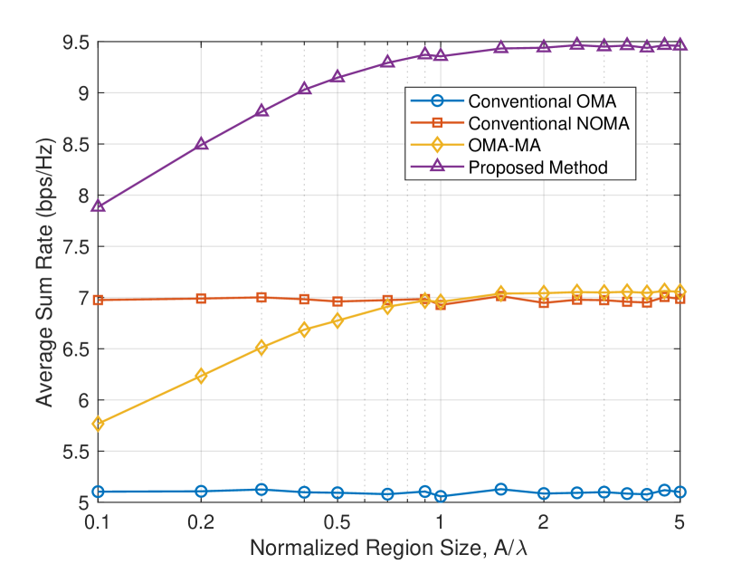
Figure 2: Average sum rate versus normalized region size.

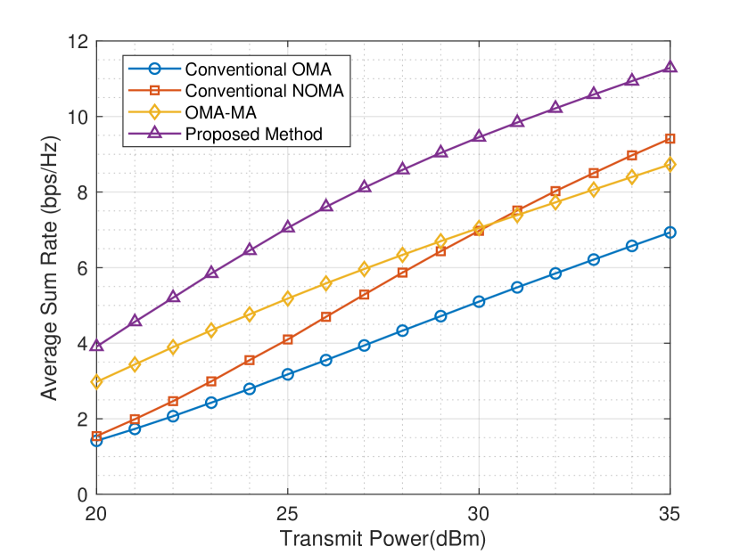
Figure 3: Average sum rate versus transmit power.

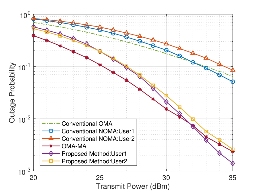
Figure 4: Outage probability versus transmit power.

In this section, we validate the proposed design through a series of numerical simulations. Specifically, we consider a communication system wherein a BS with an FPA array consisting of $N=16$ elements, catering to 2 users, each equipped with a single MA. The distances from user1 and user2 to the BS are denoted as $d_{1}=60$ m and $d_{2}=100$ m respectively. The carrier frequency utilized in downlink communication from the BS to users is 3 GHz, corresponding to a carrier wavelength of $\lambda=0.1$ m. We assume that the number of transmit paths equals that of receive paths, denoted as $L_{i}^{t}=L_{i}^{r}=L=10$. The PRM for each user is a diagonal matrix, with diagonal elements being mutually independent and conforming to the same distribution $\mathcal{CN}(0,c_{0}d^{-\beta}L^{-1})$, where $c_{0}=(\frac{\lambda}{4\pi})^{2}$ denotes the expected value of average channel gain at the reference distance of $1$ m and $\beta=2.8$ signifies the path-loss factor. Moreover, the power of AWGN received by each user is $\sigma^{2}=-90$ dBm. The elevations and azimuths of AoAs/AoDs are presumed to be independent and identically distributed, adhering to a uniform distribution over the interval $[-\frac{\pi}{2},\frac{\pi}{2}]$. The SINR threshold $\gamma_{0}=10$ dB is established to guarantee accurate decoding of the signal transmitted to each user.

We consider three baseline schemes for comparison: (1) conventional OMA, where each user utilizes an FPA and employs the OMA technique; (2) conventional NOMA, where each user employs an FPA and the NOMA technique; and (3) OMA-MA, where each user incorporates an MA and utilizes the OMA technique.

Fig. 2 illustrates the achievable average sum rate for each scheme in relation to the normalized region size. With the BS’s transmit power set at $P=30$ dBm, it is evident that the average sum rates increase alongside the normalized region size for both our proposed method and OMA-MA. This phenomenon can be attributed to the heightened channel gain attainable by adjusting the MA position as the normalized region size expands. Additionally, it is notable that the average sum rate for these two schemes tend to stabilize once the normalized region size reaches 1. This observation provides a useful reference point for setting the region size. It is noteworthy that the average sum rate tends to converge once the normalized region size reaches 1 for both conventional NOMA and OMA-MA. This convergence implies that the sum rate gain achieved by optimizing the channel response is comparable to that attained through the application of NOMA technique under this circumstance. Among all schemes considered, our proposed method demonstrates the highest achievable average sum rate within the same normalized region size.

Fig. 3 shows the achievable sum rate for each scheme versus the transmit power of the BS. When considering a set of $A=3\lambda$, it can be seen that the achievable average sum rates increase across all schemes with the rise in transmit power. This augmentation can be ascribed to the heightened SINR achieved by increasing the transmit power. Notably, the average sum rate for conventional NOMA falls below that of OMA-MA at low transmit power, but the trend reverses at high transmit power levels. This observation suggests that the performance of conventional NOMA is inferior to that of OMA with MA due to the high outage probability of NOMA. However, the potential of NOMA adoption becomes more apparent when transmit power is ample. Similarly, our proposed method exhibits the highest average sum rate among all schemes at equivalent transmit power levels.

Finally, Fig. 4 exhibits the variation in outage probabilities for user1 and user2 concerning transmit power under the setup where $A=3\lambda$, comparing all schemes. An essential concern is that outage probabilities for NOMA users are expected to surpass those employing OMA when channel condition degrade. It is noted that our proposed method illustrates a swifter decline in outage probabilities for both users as transmit power increases, resulting in lower probabilities overall. Consequently, the adoption of our proposed design accelerates the stability of the downlink communication system compared to conventional NOMA.

V Conclusion

In this paper, we considered an MA-assisted NOMA downlink communication system wherein a BS is equipped with FPAs and users possess a single MA. We focused on maximization of the channel capacity by joint optimization of power allocation and antenna positions. We presented an efficient algorithm leveraging the principle of AO and SCA to tackle this non-convex problem. Simulation results illustrated our proposed design can achieve better channel sum rate and lower outage probability than that of conventional systems.

References

• [1] J. R. Bhat, and S. A. Alqahtani, β€œ6G ecosystem: Current status and future perspective,” IEEE Access, vol. 9, pp. 43134-43167, Jan. 2021.
• [2] Q. Wu, S. Zhang, B. Zheng, C. You, and R. Zhang, β€œIntelligent reflecting surface-aided wireless communications: A tutorial,” IEEE Trans. Commun., vol. 69, no. 5, pp. 3313-3351, May 2021.
• [3] Z. Zhang, W. Chen, Q. Wu, Z. Li, X. Zhu, and J. Yuan, β€œIntelligent omni surfaces assisted integrated multi-target sensing and multi-user MIMO communications,” IEEE Trans. Commun., early access, doi: 10.1109/TCOMM.2024.3374351.
• [4] X. Zhu et al., β€œPerformance analysis of RIS-aided double spatial scattering modulation for mmWave MIMO systems,” IEEE Trans. Wireless Commun., early access, doi: 10.1109/TWC.2023.3330341.
• [5] F. Wang, W. Chen, H. Tang, and Q. Wu, β€œJoint optimization of user association, subchannel allocation, and power allocation in multi-cell multi-association OFDMA heterogeneous networks,” IEEE Trans. Commun., vol. 65, no. 6, pp. 2672-2684, Jun. 2017.
• [6] L. Zhu, W. Ma, and R. Zhang, β€œModeling and performance analysis for movable antenna enabled wireless communications,” IEEE Trans. Wireless Commun., early access, doi: 10.1109/TWC.2023.3330887.
• [7] L. Zhu, W. Ma, and R. Zhang, β€œMovable antennas for wireless communication: Opportunities and challenges,” IEEE Commun. Mag., early access, doi: 10.1109/MCOM.001.2300212.
• [8] W. Ma, L. Zhu, and R. Zhang, β€œMIMO capacity characterization for movable antenna systems,” IEEE Trans. Wireless Commun., vol. 23, no. 4, pp. 3392-3407, Apr. 2024.
• [9] H. Qin, W. Chen, Z. Li, Q. Wu, N. Cheng, and F. Chen, β€œAntenna positioning and beamforming design for fluid antenna-assisted multi-user downlink communications,” IEEE Wireless Commun. Lett., vol. 13, no. 4, pp. 1073-1077, Apr. 2024.
• [10] Z. Cheng, N. Li, J. Zhu, X. She, C. Ouyang, and P. Chen, β€œSum-rate maximization for fluid antenna enabled multiuser communications,” IEEE Commun. Lett., vol. 28, no. 5, pp. 1206-1210, May 2024.
• [11] Y. Liu, Z. Qin, M. Elkashlan, Z. Ding, A. Nallanathan, and L. Hanzo, β€œNonorthogonal multiple access for 5G and beyond,” Proc. IEEE, vol. 105, no. 12, pp. 2347-2381, Dec. 2017.
• [12] Y. Liu et al., β€œEvolution of NOMA toward next generation multiple access (NGMA) for 6G,” IEEE J. Sel. Areas Commun., vol. 40, no. 4, pp. 1037-1071, Apr. 2022.
• [13] A. Huang, L. Guo, X. Mu, C. Dong, and Y. Liu, β€œCoexisting passive RIS and active relay-assisted NOMA systems,” IEEE Trans. Wireless Commun., vol. 22, no. 3, pp. 1948-1963, Mar. 2023.
• [14] Z. Ding, Z. Yang, P. Fan, and H. V. Poor, β€œOn the performance of non-orthogonal multiple access in 5G systems with randomly deployed users,” IEEE Signal Process. Lett., vol. 21, no. 12, pp. 1501-1505, Dec. 2014.
• [15] Y. Liu, Z. Ding, M. Elkashlan, and H. V. Poor, β€œCooperative non-orthogonal multiple access with simultaneous wireless information and power transfer,” IEEE J. Sel. Areas Commun., vol. 34, no. 4, pp. 938-953, Apr. 2016.