Differentially-Private Distributed Model Predictive Control of Linear Discrete-Time Systems with Global Constraints

Abstract

Distributed model predictive control (DMPC) has attracted extensive attention as it can explicitly handle system constraints and achieve optimal control in a decentralized manner. However, the deployment of DMPC strategies generally requires the sharing of sensitive data among subsystems, which may violate the privacy of participating systems. In this paper, we propose a differentially-private DMPC algorithm for linear discrete-time systems subject to coupled global constraints. Specifically, we first show that a conventional distributed dual gradient algorithm can be used to address the considered DMPC problem but cannot provide strong privacy preservation. Then, to protect privacy against the eavesdropper, we incorporate a differential-privacy noise injection mechanism into the DMPC framework and prove that the resulting distributed optimization algorithm can ensure both provable convergence to a global optimal solution and rigorous $\epsilon$-differential privacy. In addition, an implementation strategy of the DMPC is designed such that the recursive feasibility and stability of the closed-loop system are guaranteed. Numerical simulation results confirm the effectiveness of the proposed approach.

1 Introduction

Over the past decades, model predictive control (MPC) has enjoyed great success due to its ability to explicitly handle system constraints and guarantee prescribed control performance (Mayne, 2014; Christofides et al., 2013). MPC can be implemented either in a centralized or distributed manner. Centralized MPC relies on a central unit to process all system information and solve the online optimization problem, which often results in poor scalability and requires substantial computation power, especially for complex or large-scale systems. Consequently, distributed MPC (DMPC) has garnered much attention in recent years, offering many advantages of distributed systems and proving to be an effective tool for various applications, including vehicle platoons (Zheng et al., 2016), microgrids (Hans et al., 2018), and multi-robot systems (Luis et al., 2020).

Based on the type of couplings between subsystems, DMPC studies can be roughly divided into three categories, i.e., coupling in cost functions, coupling in system dynamics, and coupling in constraints. In this paper, we focus on systems with coupled global constraints, which have many real-world applications (Bai et al., 2023; Michos et al., 2022). Several approaches have been proposed to guarantee the strict satisfaction of coupled constraints in a distributed manner. In Richards and How (2007), a sequential DMPC method is developed, which first divides the global problem into several local subproblems and then solves them sequentially in a given order. The satisfaction of coupled constraints is guaranteed through plan exchanges among subsystems. Trodden and Richards (2010) proposes a DMPC approach for flexible communication that can remove optimization order restrictions. Building on Richards and How (2007) and Trodden and Richards (2010), Trodden (2014) presents a parallel DMPC approach allowing simultaneous optimizations and maintaining flexible communication and parallel computation advantages. However, global optimality remains unclear in these approaches. In Wang and Ong (2017), a dual decomposition-based DMPC approach is designed to explicitly pursue global optimality. This approach transforms the dual problem of DMPC into a consensus optimization problem and then solves it using the distributed alternating direction multiplier method (ADMM). To improve the convergence speed when solving DMPC, a Nesterov-accelerated-gradient algorithm is utilized in Wang and Ong (2018). In addition, a push-sum dual gradient algorithm and a noisy ADMM algorithm are developed in Jin et al. (2020) and Li et al. (2021) to address the DMPC problem under time-varying directed communication network and communication noise, respectively.

In the aforementioned methods (Wang and Ong, 2017, 2018; Jin et al., 2020; Li et al., 2021), distributed optimization algorithms are leveraged to address the DMPC problem, requiring each subsystem/agent to share explicit local information with neighboring subsystems/agents in order to satisfy coupled global constraints. Note that the shared messages often contain sensitive information, which raises significant concerns about privacy leakage. For instance, an eavesdropper could wiretap the communication channel and deduce privacy-sensitive information from exchanged messages. When DMPC is adopted in specific domains like smart grid or intelligent transportation, the disclosure of privacy-sensitive information may further pose safety risks and lead to economic losses. Considering the growing awareness of privacy and security, it is imperative to ensure privacy protection in DMPC. So far, few results are available on the privacy preservation of DMPC, but privacy-preserving approaches for distributed optimization have been well studied. For the latter, one typical technique is (partially) homomorphic encryption, which has been employed in Lu and Zhu (2018); Zhang and Wang (2018). The encryption-based methods use cryptography to mask privacy-sensitive information and can be directly extended for the privacy protection of DMPC (Zhao et al., 2023). However, this technique generally requires tedious encryption and decryption procedures, leading to huge overheads in both communication and computation. Another technique relies on spatially or temporally correlated noises/uncertainties (Gade and Vaidya, 2018; Lou et al., 2017; Gao et al., 2023), aiming to obscure information shared in distributed optimization. Due to the correlated nature of these noises/uncertainties, these approaches are typically vulnerable to adversaries with access to all messages shared in the network.

With implementation simplicity and rigorous mathematical foundations, differential privacy (DP) has witnessed growing popularity, emerging as a de facto standard for privacy protection. In recent years, DP-based privacy methods have been introduced in distributed optimization by injecting DP noise to objective functions (Nozari et al., 2016) or exchanged information (Huang et al., 2015; Xiong et al., 2020; Ding et al., 2021). Nevertheless, the direct integration of persistent DP noise into existing algorithms inevitably compromises optimization accuracy, resulting in a fundamental trade-off between privacy and accuracy. It is crucial to note that extending DP-based privacy approaches to DMPC is not straightforward, as the compromise on optimization accuracy can deteriorate control performance and potentially lead to constraint violations.

In this paper, a differentially-private DMPC algorithm is designed for linear discrete-time systems with coupled global constraints. We first demonstrate the need for privacy preservation by showcasing that a conventional distributed dual gradient algorithm for DMPC is vulnerable to eavesdropping attacks. A DP noise injection mechanism is then introduced into the distributed dual gradient algorithm, which obscures the private information exchanged among subsystems to prevent adversaries from inferring sensitive information. By leveraging the results in Wang (2023); Wang and Nedić (2024), a weakening factor sequence and a step-size sequence are carefully designed to effectively mitigate the influence of DP noise. Rigorous analysis shows that the proposed algorithm can ensure almost sure convergence to a global optimal solution and maintain $\epsilon$-differential privacy with a finite cumulative privacy budget. Aligned with the privacy-preserving distributed algorithm, we provide an implementation strategy for DMPC, ensuring the recursive feasibility and stability of the closed-loop system. Simulations are performed to validate the performance of the proposed scheme.

The rest of the paper is organized as follows. In Section 2, the preliminaries of DMPC and differential privacy are introduced. In Section 3, a novel differentially-private distributed dual gradient algorithm is designed, and convergence analysis is conducted. In Section 4, the implementation strategy of DMPC is presented. Finally, a numerical study is given in Section 5, and concluding remarks are summarized in Section 6.

Notations: $\mathbb{R}^{n}$ stands for the $n$-dimensional Euclidean space. Given two integers $a$ and $b$ ($a<b$), $\mathbb{Z}_{a}^{b}$ represents the set $\{a,a+1,\cdots,b\}$. $I_{n}$ denotes the identify matrix of dimension $n$. ${\bf 1}_{n}$ and ${\bf 0}_{n}$ represent the $n$-dimensional column vector with all entries equal to 1 and 0, respectively. We use $Q>(\geq)0$ to denote that $Q$ is a positive definite (semi-definite) matrix. $\|x\|$ and $\|x\|_{1}$ represent the standard Euclidean norm and the $L_{1}$ norm of a vector $x$, respectively. Moreover, $\|x\|_{Q}^{2}:=x^{\top}Qx$.

2 Problem Formulation and Preliminaries

2.1 Problem Description

Consider $M$ linear discrete-time subsystems where each is described as follows:

$$x_{i}(t+1)=A_{i}x_{i}(t)+B_{i}u_{i}(t),\quad i\in\mathbb{Z}_{1}^{M}.$$ (1)

In (1), $x_{i}(t)\in\mathbb{R}^{n_{i}}$ and $u_{i}(t)\in\mathbb{R}^{m_{i}}$ are the state and control input of subsystem $i$ at time instant $t$, respectively. The state and control input of subsystem $i$ should satisfy the following local constraints:

$$x_{i}(t)\in\mathcal{X}_{i},\quad u_{i}(t)\in\mathcal{U}_{i},$$ (2)

where $\mathcal{X}_{i}\subset\mathbb{R}^{n_{i}}$ and $\mathcal{U}_{i}\subset\mathbb{R}^{m_{i}}$ are state and control input constraint sets, respectively. Moreover, all the subsystems are subject to $p$ global constraints described by

$$\sum_{i=1}^{M}(\varPsi_{x_{i}}x_{i}(t)+\varPsi_{u_{i}}u_{i}(t))\leq{\bf 1}_{p},$$ (3)

where $\varPsi_{x_{i}}\in\mathbb{R}^{p\times n_{i}}$ and $\varPsi_{u_{i}}\in\mathbb{R}^{p\times m_{i}}$ are some given matrices.

Assumption 1.

Each linear discrete-time subsystem, i.e., $(A_{i},B_{i})$, is controllable. Additionally, $\mathcal{X}_{i}$ and $\mathcal{U}_{i}$ are bounded and closed polytopes containing the origins as their inner point.

In this paper, we consider the same DMPC optimization problem as presented in Wang and Ong (2017, 2018); Jin et al. (2020); Li et al. (2021); Zhao et al. (2023). Specifically, based on (1)-(3), the DMPC optimization problem is formulated as

$$\mathcal{P}:\quad \min_{\{\tilde{{\bm{u}}}_{1},\cdots,\tilde{{\bm{u}}}_{M}\}}\sum_{i=1}^{M}J_{i}(x_{i}(t),\tilde{{\bm{u}}}_{i})$$ (4a)

$$\;\mathrm{s.t.}\quad\tilde{{\bm{u}}}_{i}\in\tilde{\mathcal{U}_{i}}(x_{i}(t))$$ (4b)

$$\quad\quad\sum_{i=1}^{M}f_{i}(x_{i}(t),\tilde{{\bm{u}}}_{i})\leq b(\varepsilon).$$ (4c)

In (4a), $J_{i}(x_{i}(t),\tilde{{\bm{u}}}_{i})$ is the local objective function, which is defined as

$$J_{i}(x_{i}(t),\tilde{{\bm{u}}}_{i}):=\sum_{\ell=0}^{N-1}\left(\|\tilde{x}_{i}(\ell|t)\|_{Q_{i}}^{2}+\|\tilde{u}_{i}(\ell|t)\|_{R_{i}}^{2}\right)+\|\tilde{x}_{i}(N|t)\|_{P_{i}}^{2},$$ (5)

where $N\in\mathbb{Z}_{>0}$ is the length of prediction horizon, $\tilde{x}_{i}(\ell|t)$ and $\tilde{u}_{i}(\ell|t)$ are the $\ell$th step-predicted state and control input at time instant $t$, respectively, $\tilde{{\bm{u}}}_{i}:=\{\tilde{u}_{i}(0|t),\cdots,\tilde{u}_{i}(N-1|t)\}$ stands for the predicted input sequence over the prediction horizon, and $Q_{i}>0$, $R_{i}>0$, and $P_{i}>0$ are weight matrices. For each subsystem $i$, $P_{i}$ is the solution of the algebraic Riccati equation

$$(A_{i}+B_{i}K_{i})^{\top}P_{i}(A_{i}+B_{i}K_{i})-P_{i}=-(Q_{i}+K_{i}^{\top}R_{i}K_{i}),$$ (6)

where $K_{i}:=-(R_{i}+B_{i}^{\top}P_{i}B_{i})^{-1}B_{i}^{\top}P_{i}A_{i}$. The local constraint set $\tilde{\mathcal{U}_{i}}(x_{i}(t))$ in (4b) is defined as

$$\tilde{\mathcal{U}_{i}}(x_{i}(t)):=\{\tilde{{\bm{u}}}_{i}\in\mathbb{R}^{m_{i}N}:\tilde{x}_{i}(\ell+1|t)=A_{i}\tilde{x}_{i}(\ell|t)+B_{i}\tilde{u}_{i}(\ell|t),$$ (7)

$$\tilde{x}_{i}(0|t)=x_{i}(t),\tilde{x}_{i}(\ell|t)\in\mathcal{X}_{i},\tilde{u}_{i}(\ell|t)\in\mathcal{U}_{i},\tilde{x}_{i}(N|t)\in\mathcal{X}_{i}^{f},\ell\in\mathbb{Z}_{0}^{N-1}\},$$

with $\mathcal{X}_{i}^{f}$ being the terminal constraint set. In addition, the global coupled constraint in (4c) is a tightened form of the constraint in (3), and $f_{i}(x_{i}(t),\tilde{{\bm{u}}}_{i})$ and $b(\varepsilon)$ are given by

$$f_{i}(x_{i}(t),\tilde{{\bm{u}}}_{i}) :=\begin{bmatrix}\varPsi_{x_{i}}\tilde{x}_{i}(0|t)+\varPsi_{u_{i}}\tilde{u}_{i}(0|t)\\ \vdots\\ \varPsi_{x_{i}}\tilde{x}_{i}(N-1|t)+\varPsi_{u_{i}}\tilde{u}_{i}(N-1|t)\end{bmatrix},$$ (8)

$$b(\varepsilon) :=\begin{bmatrix}(1-\varepsilon M){\bf 1}_{p}\\ \vdots\\ (1-\varepsilon MN){\bf 1}_{p}\end{bmatrix},$$

where $0\leq\varepsilon<\frac{1}{MN}$ is a tolerance parameter. The introduction of the tightened constraint is to ensure that the numerical algorithm used to solve the DMPC problem can be terminated in advance. To facilitate the feasibility and stability analysis of DMPC, the terminal constraint set $\mathcal{X}_{i}^{f}$ can be chosen as a closed maximal polytope such that for any $x_{i}\in\mathcal{X}_{i}^{f}$, we have

$$K_{i}x_{i}\in\mathcal{U}_{i},\quad(A_{i}+B_{i}K_{i})x_{i}\in\mathcal{X}_{i}^{f},$$ (9)

$$\sum_{i=1}^{M}(\varPsi_{x_{i}}+\varPsi_{u_{i}}K_{i})x_{i}\leq(1-\varepsilon MN){\bf 1}_{p}.$$

For more details about the tightening of constraint (3) and the construction of the terminal constraint set $\mathcal{X}_{i}^{f}$, please refer to Wang and Ong (2017).

Assumption 2.

For the initial system state $\{x_{1}(0),\cdots,x_{M}(0)\}$, the Slater condition holds, i.e., there exists $\{\tilde{{\bm{u}}}_{1},\cdots,\tilde{{\bm{u}}}_{M}\}$ that satisfies (4b) and (4c).

The communication network of $M$ subsystems is described by an interaction weight matrix $L=\{L_{ij}\}\in\mathbb{R}^{M\times M}$. Specifically, for each subsystem $i$, its neighbor set $\mathcal{N}_{i}$ is defined as the collections of subsystems $j$ such that subsystem $i$ and subsystem $j$ can directly communicate with each other. If $j\in\mathcal{N}_{i}$, then $L_{ij}>0$; otherwise, $L_{ij}=0$. We define $L_{ii}:=-\sum_{j\in\mathcal{N}_{i}}L_{ij}$ for all $i\in\mathbb{Z}_{1}^{M}$. Moreover, $L$ satisfies the following assumption:

Assumption 3.

The matrix $L=\{L_{ij}\}$ is symmetric and satisfies ${\bf 1}_{M}^{\top}L={\bf 0}_{M}^{\top}$, $L{\bf 1}_{M}={\bf 0}_{M}$, and $\|I_{M}+L-\frac{{\bf 1}_{M}{\bf 1}_{M}^{\top}}{M}\|<1$.

Assumption 3 ensures that the communication graph induced by $L$ is connected, i.e., there is a path from any subsystem to any other subsystem.

2.2 Distributed Dual-Gradient Method

The Lagrangian function associated with the optimization problem in (4) is given by

$$\mathcal{L}(\{\tilde{{\bm{u}}}_{i}\},\lambda) =\sum_{i=1}^{M}J_{i}(x_{i}(t),\tilde{{\bm{u}}}_{i})+\lambda^{\top}\left(\sum_{i=1}^{M}f_{i}(x_{i}(t),\tilde{{\bm{u}}}_{i})-b(\varepsilon)\right)$$ (10)

$$=\sum_{i=1}^{M}\left(J_{i}(x_{i}(t),\tilde{{\bm{u}}}_{i})+\lambda^{\top}g_{i}(\tilde{{\bm{u}}}_{i})\right),$$

where $\lambda\in\mathbb{R}^{Np}_{+}$ (the non-negative orthant of $\mathbb{R}^{Np}$) is the Lagrangian multiplier and $g_{i}(\tilde{{\bm{u}}}_{i}):=f_{i}(x_{i}(t),\tilde{{\bm{u}}}_{i})-\frac{b(\varepsilon)}{M}$. The dual problem of (4) is defined as

$$\max_{\lambda\geq 0}\min_{\{\tilde{{\bm{u}}}_{i}\in\tilde{\mathcal{U}_{i}}(x_{i}(t))\}}\mathcal{L}(\{\tilde{{\bm{u}}}_{i}\},\lambda).$$ (11)

Based on Assumptions 1, 2 and the definition of DMPC problem, it can be concluded that the strong duality holds for (4), and the optimization problem (4) can be addressed by solving its dual problem (11). In addition, the Saddle-Point Theorem holds, i.e., given an optimal primal-dual pair $(\{\tilde{{\bm{u}}}_{i}^{*}\},\lambda^{*})$, we have

$$\mathcal{L}(\{\tilde{{\bm{u}}}_{i}^{*}\},\lambda)\leq\mathcal{L}(\{\tilde{{\bm{u}}}_{i}^{*}\},\lambda^{*})\leq\mathcal{L}(\{\tilde{{\bm{u}}}_{i}\},\lambda^{*}),\;\lambda\in\mathbb{R}^{Np}_{+},\;\tilde{{\bm{u}}}_{i}\in\tilde{\mathcal{U}_{i}}(x_{i}(t)).$$ (12)

A conventional approach to solving problem (11) is the distributed dual-gradient method (Falsone et al., 2017; Notarstefano et al., 2019). The core idea is to regard the Lagrangian multiplier (dual variable) $\lambda$ as a consensus variable and then $M$ subsystems address the optimization problem in a collective manner. Specifically, let each subsystem have a local copy $\lambda_{i}^{k}$ of the dual variable. $\Pi_{\mathbb{R}^{Np}_{+}}\left[\cdot\right]$ denotes Euclidean projection of a vector on the set $\mathbb{R}^{Np}_{+}$, and $\gamma^{k}>0$ denotes the step-size. Then, the distributed dual-gradient method is summarized in Algorithm 1, and the overall DMPC implementation is detailed in Algorithm 2.

Input: $x_{i}(t)$, $i\in\mathbb{Z}_{1}^{M}$

Output: $\tilde{{\bm{u}}}_{i}^{\bar{k}}$, $i\in\mathbb{Z}_{1}^{M}$

1 Initialization: set $\lambda_{i}^{0}\in\mathbb{R}^{Np}_{+}$ and $\tilde{{\bm{u}}}_{i}^{0}\in\tilde{\mathcal{U}_{i}}(x_{i}(t))$, $\forall i\in\mathbb{Z}_{1}^{M}$ Parameters: deterministic sequence $\gamma^{k}>0$

2for $k=0,2,\cdots,\bar{k}-1$ do

3       for all $i\in\mathbb{Z}_{1}^{M}$ (in parallel) do

4             Every subsystem $i$ sends $\lambda_{i}^{k}$ to subsystem $j\in\mathcal{N}_{i}$;

5             After receiving $\lambda_{j}^{k}$ from all $j\in\mathcal{N}_{i}$, subsystem $i$ updates its primal and dual variables:

$$\tilde{\lambda}_{i}^{k}=\lambda_{i}^{k}+\sum_{j\in\mathcal{N}_{i}}L_{ij}(\lambda_{j}^{k}-\lambda_{i}^{k});$$ (13)

$$\tilde{{\bm{u}}}_{i}^{k+1}=\mathop{\rm argmin}_{\tilde{{\bm{u}}}_{i}\in\tilde{\mathcal{U}_{i}}(x_{i}(t))}J_{i}(x_{i}(t),\tilde{{\bm{u}}}_{i})+(\tilde{\lambda}_{i}^{k})^{\top}g_{i}(\tilde{{\bm{u}}}_{i});$$ (14)

$$\lambda_{i}^{k+1}=\Pi_{\mathbb{R}^{Np}_{+}}\left[\tilde{\lambda}_{i}^{k}+\gamma^{k}g_{i}(\tilde{{\bm{u}}}_{i}^{k+1})\right];$$ (15)

6       end for

7      

8 end for

Algorithm 1 Distributed Dual-gradient Algorithm

1 At time instant $t$, each subsystem $i$ measures its state $x_{i}(t)$;

2Each subsystem $i$ obtains $\tilde{{\bm{u}}}_{i}^{\bar{k}}$ by following Algorithm 1 with $x_{i}(t)$;

3Set the input sequence as $\tilde{{\bm{u}}}_{i}(t)=\tilde{{\bm{u}}}_{i}^{\bar{k}}$;

4Apply $\tilde{u}_{i}(0|t)$ to subsystem $i$;

Wait for the next sampling instant; let $t=t+1$ and go to step 1.

Algorithm 2 DMPC Algorithm

If Assumptions 2 and 3 hold and if the step-size $\gamma^{k}$ satisfies the conditions $\sum_{k=0}^{\infty}\gamma^{k}=\infty$, $\sum_{k=0}^{\infty}(\gamma^{k})^{2}<\infty$, then Algorithm 1 guarantees the convergence of the sequence $\{\tilde{{\bm{u}}}_{i}^{k}\}$, i.e., $\lim_{k\rightarrow\infty}\|\tilde{{\bm{u}}}_{i}^{k}-\tilde{{\bm{u}}}_{i}^{*}\|$. Note that the objective function of problem (4) is strictly convex, and thus the asymptotic primal convergence can be established without resorting to local averaging mechanism (see Section 3.4 in Notarstefano et al. (2019) for more details). In addition, if the iteration number $\bar{k}$ is selected sufficiently large to meet specific criteria (Su et al., 2022; Wang and Ong, 2017), then Algorithm 2 ensures the feasibility and stability of the considered MPC problem.

In Algorithm 1, each subsystem can avoid sharing the primal variable and only share its local copy $\lambda_{i}^{k}$ of the dual variable with its neighbors. However, this sharing mechanism cannot provide strong privacy protection as the iteration trajectory of $\lambda_{i}^{k}$ still bears information of the primal variable. In particular, we assume that the adversary has prior knowledge about the communication network $L$ and the step-size $\gamma^{k}$, and can get access to all information exchanged in communication channels. Under this circumstance, the adversary can record the updates of $\bar{\lambda}_{i}^{k}$ and $\lambda_{i}^{k}$ at each iteration. Then, based on $\bar{\lambda}_{i}^{k}$ and $\lambda_{i}^{k+1}$ in two consecutive iterations and $\gamma^{k}$, the adversary can employ (15) to estimate the value of $g_{i}(\tilde{{\bm{u}}}_{i}^{k+1})$. It should be noted that $g_{i}(\tilde{{\bm{u}}}_{i}^{k+1})$ is privacy-sensitive as it is the function of primal variable and is used to formulate the coupled global constraint. Therefore, it is necessary to incorporate a privacy protection mechanism into the distributed dual-gradient algorithm such that the DMPC problem can be addressed with privacy protection.

2.3 On Differential Privacy

In this work, DP is used to characterize and quantify the achieved privacy level of distributed optimization algorithms. Given the continual exchange of information among subsystems in iterative optimization algorithms, the notion of $\epsilon$-DP for continuous bit streams (Dwork et al., 2010) is adopted. Drawing inspiration from the distributed optimization framework proposed by Huang et al. (2015), we represent the DMPC problem in (4) by four parameters $(\mathcal{J},\tilde{\mathcal{U}},\mathcal{G},L)$ to facilitate DP analysis. Specifically, $\mathcal{J}:=\{J_{1},\,\cdots,J_{M}\}$ denotes the set of objective functions for individual subsystems, $\tilde{\mathcal{U}}:=\{\tilde{\mathcal{U}_{1}},\cdots,\tilde{\mathcal{U}_{M}}\}$ is the domain of optimization variables, $\mathcal{G}:=\{g_{1},\cdots,g_{M}\}$ represents the set of constraint functions for individual subsystems, and $L$ is the weight matrix describing the communication network. The adjacency between two optimization problems is defined as follows:

Definition 1.

Two optimization problems $\mathcal{P}=(\mathcal{J},\tilde{\mathcal{U}},\mathcal{G},L)$ and $\mathcal{P}^{{}^{\prime}}=(\mathcal{J}^{{}^{\prime}},\tilde{\mathcal{U}}^{{}^{\prime}},\mathcal{G}^{{}^{\prime}},L^{{}^{\prime}})$ are adjacent if the following conditions hold:

• the objective functions, the domains of optimization variables, and the interaction weight matrices are identical, i.e., $\mathcal{J}=\mathcal{J}^{{}^{\prime}}$, $\tilde{\mathcal{U}}=\tilde{\mathcal{U}}^{{}^{\prime}}$, and $L=L^{{}^{\prime}}$;

• there exists an $i\in\mathbb{Z}_{1}^{M}$ such that $g_{i}\neq g_{i}^{{}^{\prime}}$ but $g_{j}=g_{j}^{{}^{\prime}}$ for all $j\in\mathbb{Z}_{1}^{M},\,j\neq i$;

• $g_{i}$ and $g_{i}^{{}^{\prime}}$, which are not the same, have similar behaviors around $\theta^{*}$, the solution of $\mathcal{P}$. More specifically, there exists some $\delta>0$ such that for all $\bm{u}_{i}$ and $\bm{u}_{i}^{{}^{\prime}}$ in $B_{\delta}(\theta^{*}):=\{\bm{v}:\bm{v}\in\mathbb{R}^{Nm_{i}},\|\bm{v}-\theta^{*}\|<\delta\}$, we have $g_{i}(\bm{u}_{i})=g_{i}^{{}^{\prime}}(\bm{u}_{i}^{{}^{\prime}})$.

In the context of a distributed optimization algorithm, we denote an execution of such an algorithm as $\mathcal{A}$, represented by a sequence of the iteration variable $\vartheta$, i.e., $\mathcal{A}=\{\vartheta^{0},\vartheta^{1},\cdots\}$. We consider adversaries that can get access to all communicated messages among the subsystems. Hence, under an execution $\mathcal{A}$, the observation of adversaries is the sequence of shared messages, which is denoted as $\mathcal{O}$. For a given distributed optimization problem $\mathcal{P}$ and an initial state $\vartheta^{0}$, we define the observation mapping as $\mathcal{R}_{\mathcal{P},\vartheta^{0}}(\mathcal{A}):=\mathcal{O}$. Given a distributed optimization problem $\mathcal{P}$, an observation sequence $\mathcal{O}$, and an initial state $\vartheta^{0}$, $\mathcal{R}_{\mathcal{P},\vartheta^{0}}^{-1}(\mathcal{O})$ denotes the set of executions $\mathcal{A}$ capable of generating the observation $\mathcal{O}$.

Definition 2 ($\epsilon$-differential privacy, Huang et al. (2015)).

For a given $\epsilon>0$, an iterative distributed algorithm is $\epsilon$-differentially private if for any two adjacent $\mathcal{P}$ and $\mathcal{P}^{\prime}$, any set of observation sequences $\mathcal{O}_{s}\subseteq\mathbb{O}$ (with $\mathbb{O}$ denoting the set of all possible observation sequences), and any initial state ${\vartheta}^{0}$, the following relationship always holds

$$\mathbb{P}[\mathcal{R}_{\mathcal{P},\vartheta^{0}}\left(\mathcal{O}_{s}\right)]\leq e^{\epsilon}\mathbb{P}[\mathcal{R}_{\mathcal{P}^{{}^{\prime}},\vartheta^{0}}\left(\mathcal{O}_{s}\right)],$$ (16)

with the probability $\mathbb{P}$ taken over the randomness over iteration processes.

The definition of $\epsilon$-DP guarantees that adversaries, with access to all shared messages, cannot gain knowledge about any participating subsystem’s sensitive information. It can be seen that a smaller $\epsilon$ means a higher level of privacy protection.

3 Differentially-Private Distributed Dual-Gradient Algorithm

3.1 Algorithm Description

In this section, a DP noise injection mechanism is proposed to achieve privacy preservation in the distributed dual-gradient algorithm. The developed algorithm is summarized in Algorithm 3.

In contrast to Algorithm 1, where each subsystem directly sends $\lambda_{i}^{k}$ to its neighbors, Algorithm 3 incorporates DP noise $\zeta_{i}^{k}$ into $\lambda_{i}^{k}$ and shares the perturbed signal $\hat{\lambda}_{i}^{k}:=\lambda_{i}^{k}+\zeta_{i}^{k}$ among the communication network. Therefore, the information available to potential adversaries is the sequence $\{\hat{\lambda}_{i}^{k}\}$. Due to the randomness of DP noise, it is impossible for the adversary to extract useful information from $\{\hat{\lambda}_{i}^{k}\}$ with significant probability. Furthermore, it should be noted that directly integrating persistent DP noise into existing optimization algorithms will compromise the convergence accuracy. To address this issue, we utilize findings from Wang (2023); Wang and Nedić (2024) to design a weakening factor. As shown in (18), the weakening factor, denoted as $\chi^{k}$, is applied on the interaction terms ($L_{ij}(\hat{\lambda}_{j}^{k}-\lambda_{i}^{k})$). The fundamental principle behind incorporating this weakening factor is to gradually eliminate the impact of DP noise on convergence accuracy.

Input: $x_{i}(t)$, $i\in\mathbb{Z}_{1}^{M}$

Output: $\tilde{{\bm{u}}}_{i}^{\bar{k}}$, $i\in\mathbb{Z}_{1}^{M}$

1 Initialization: set $\lambda_{i}^{0}\in\mathbb{R}^{Np}_{+}$ and $\tilde{{\bm{u}}}_{i}^{0}\in\tilde{\mathcal{U}_{i}}(x_{i}(t))$, $\forall i\in\mathbb{Z}_{1}^{M}$ Parameters: deterministic sequence $\gamma^{k}>0$ and $\chi^{k}>0$

2for $k=0,2,\cdots,\bar{k}-1$ do

3       for all $i\in\mathbb{Z}_{1}^{M}$ (in parallel) do

4             Every subsystem $i$ adds DP noise $\zeta_{i}^{k}$ to $\lambda_{i}^{k}$, and then sends the obscured value $\hat{\lambda}_{i}^{k}:=\lambda_{i}^{k}+\zeta_{i}^{k}$ to subsystem $j\in\mathcal{N}_{i}$;

5             After receiving $\hat{\lambda}_{j}^{k}$ from all $j\in\mathcal{N}_{i}$, subsystem $i$ updates its primal and dual variables:

$$\tilde{{\bm{u}}}_{i}^{k+1}=\mathop{\rm argmin}_{\tilde{{\bm{u}}}_{i}\in\tilde{\mathcal{U}_{i}}(x_{i}(t))}J_{i}(x_{i}(t),\tilde{{\bm{u}}}_{i})+(\lambda_{i}^{k})^{\top}g_{i}(\tilde{{\bm{u}}}_{i});$$ (17)

$$\lambda_{i}^{k+1}=\Pi_{\mathbb{R}^{Np}_{+}}\left[\lambda_{i}^{k}+\chi^{k}\sum_{j\in\mathcal{N}_{i}}L_{ij}(\hat{\lambda}_{j}^{k}-\lambda_{i}^{k})+\gamma^{k}g_{i}(\tilde{{\bm{u}}}_{i}^{k+1})\right];$$ (18)

6       end for

7      

8 end for

Algorithm 3 Differentially-private Distributed Dual-gradient Algorithm

To facilitate the convergence and privacy analysis, we make the following assumption on the DP noise:

Assumption 4.

For every $i\in\mathbb{Z}_{1}^{M}$ and every $k$, conditional on $\lambda_{i}^{k}$, the DP noise $\zeta_{i}^{k}$ satisfies $\mathbb{E}\left[\zeta_{i}^{k}\mid\lambda_{i}^{k}\right]=0$ and $\mathbb{E}\left[\|\zeta_{i}^{k}\|^{2}\mid\lambda_{i}^{k}\right]=(\sigma_{i}^{k})^{2}$ for all $k\geq 0$, and

$$\sum_{k=0}^{\infty}(\chi^{k})^{2}\,\max_{i\in\mathbb{Z}_{1}^{M}}(\sigma_{i}^{k})^{2}<\infty,$$ (19)

where $\{\chi^{k}\}$ is the weakening factor sequence from Algorithm 3. The initial random vectors satisfy $\mathbb{E}\left[\|\lambda_{i}^{0}\|^{2}\right]<\infty$, $\forall i\in\mathbb{Z}_{i}^{M}$.

Considering Assumption 4, we use the Laplace noise mechanism to generate $\zeta_{i}^{k}$, i.e., we add Laplace noise to all shared messages. More specifically, given a constant $\nu>0$, we use ${\rm Lap}(\nu)$ to denote a Laplace distribution of a scalar random variable with the probability density function being $\rho\rightarrow\frac{1}{2\nu}e^{-\frac{|\rho|}{\nu}}$. At each iteration $k$, all elements of $\zeta_{i}^{k}$ are drawn independently from Laplace distribution ${\rm Lap}(\nu^{k})$, where $\nu^{k}>0$. One can verify that the mean and variance of ${\rm Lap}(\nu^{k})$ is zero and $2(\nu^{k})^{2}$, respectively. Therefore, $\zeta_{i}^{k}$ satisfies $\mathbb{E}\left[\zeta_{i}^{k}\mid\lambda_{i}^{k}\right]=0$ and $\mathbb{E}\left[\|\zeta_{i}^{k}\|^{2}\mid\lambda_{i}^{k}\right]=(\sigma_{i}^{k})^{2}=2(\nu^{k})^{2}$.

Remark 1.

In Algorithm 3, we allow the variance of DP noise $\zeta_{i}^{k}$, i.e., $2(\nu^{k})^{2}$, to be constant or increasing with $k$. To satisfy condition (19), one can carefully design the weakening factor sequence $\{\chi^{k}\}$ to make its decreasing rate outweigh the increasing rate of the noise level sequence $\{\nu^{k}\}$. For instant, (19) can be satisfied by setting $\chi^{k}=\frac{c_{1}}{1+c_{2}k^{c_{3}}}$ and $\nu^{k}=d_{1}+d_{2}k^{d_{3}}$ with any $c_{1}>0$, $c_{2}>0$, $0.5<c_{3}<1$, $d_{1}>0$, $d_{2}>0$, and $0<d_{3}<0.5-c_{3}$.

3.2 Convergence Analysis

The arithmetic average of local dual variables $\lambda_{i}^{k}$ is given by

$$\bar{\lambda}^{k}=\frac{1}{M}\sum_{i=1}^{M}\lambda_{i}^{k}.$$ (20)

The relation between $\lambda_{i}^{k}$ and $\bar{\lambda}^{k}$ is summarized in the following theorem.

Theorem 1.

Suppose Assumptions 1, 3, and 4 hold. If the non-negative weakening factor sequence $\{\chi^{k}\}$ and the step-size sequence $\{\gamma^{k}\}$ in Algorithm 3 satisfy

$$\sum_{k=0}^{\infty}\chi^{k}=\infty,\,\sum_{k=0}^{\infty}(\chi^{k})^{2}<\infty,\,\sum_{k=0}^{\infty}\frac{(\gamma^{k})^{2}}{\chi^{k}}<\infty,$$ (21)

then the following results hold almost surely:

1. $\lim_{k\to\infty}\left\|\lambda_{i}^{k}-\bar{\lambda}^{k}\right\|=0$ for all $i\in\mathbb{Z}_{1}^{M}$;

2. $\sum_{k=0}^{\infty}\chi^{k}\sum_{i=1}^{M}\left\|\lambda_{i}^{k}-\bar{\lambda}^{k}\right\|^{2}<\infty$;

3. $\sum_{k=0}^{\infty}\gamma^{k}\sum_{i=1}^{M}\left\|\lambda_{i}^{k}-\bar{\lambda}^{k}\right\|<\infty$.

Proof.

Based on Assumption 1 and (7), it can be concluded that the local constraint set $\tilde{\mathcal{U}_{i}}(x_{i}(t))$ is bounded. Then, from (8) and the relation $g_{i}(\tilde{{\bm{u}}}_{i}):=f_{i}(x_{i}(t),\tilde{{\bm{u}}}_{i})-\frac{b(\varepsilon)}{M}$, we have that for any $\tilde{{\bm{u}}}_{i}\in\tilde{\mathcal{U}_{i}}(x_{i}(t))$, $g_{i}(\tilde{{\bm{u}}}_{i})$ is bounded, i.e., there exists a constant $C_{g}\in\mathbb{R}_{+}$ such that

$$\|g_{i}(\tilde{{\bm{u}}}_{i})\|\leq C_{g},\forall\tilde{{\bm{u}}}_{i}\in\tilde{\mathcal{U}_{i}}(x_{i}(t)),i\in\mathbb{Z}_{1}^{M}.$$ (22)

According to Assumptions 3, 4, (21), and (22), we can follow the same line of reasoning as that of Theorem 1 in Wang and Nedić (2024) to obtain the results.  

We also need the following lemma for convergence analysis:

Lemma 1 (Lemma 11, Polyak (1987)).

Let $\{\psi^{k}\}$, $\{\phi^{k}\}$, $\{a^{k}\}$, and $\{b^{k}\}$ be random non-negative scalar sequences such that

$$\mathbb{E}\left[\psi^{k+1}|\mathcal{F}^{k}\right]\leq(1+{a^{k}})\psi^{k}-\phi^{k}+{b^{k}},\quad\forall k\geq 0,$$

where $\mathcal{F}^{k}=\{\psi^{\ell},\phi^{\ell},{a^{\ell}},{b^{\ell}};\,0\leq\ell\leq k\}$. If $\sum_{k=0}^{\infty}{a^{k}}<\infty$ and $\sum_{k=0}^{\infty}{b^{k}}<\infty$, then $\sum_{k=0}^{\infty}\phi^{k}<\infty$ and $\{\psi^{k}\}$ converges to a finite variable almost surely.

Theorem 2.

Suppose Assumptions 1, 3, and 4 hold. If the non-negative sequences $\{\chi^{k}\}$ and $\{\gamma^{k}\}$ satisfy $\sum_{k=0}^{\infty}\chi^{k}=\infty$, $\sum_{k=0}^{\infty}(\chi^{k})^{2}<\infty$, $\sum_{k=0}^{\infty}\gamma^{k}=\infty$, and $\sum_{k=0}^{\infty}\frac{(\gamma^{k})^{2}}{\chi^{k}}<\infty$, then Algorithm 3 guarantees that

$$\lim_{k\rightarrow\infty}\mathcal{L}(\{\tilde{{\bm{u}}}_{i}^{*}\},\bar{\lambda}^{k})=\mathcal{L}(\{\tilde{{\bm{u}}}_{i}^{*}\},\lambda^{*}),\lim_{k\rightarrow\infty}\mathcal{L}(\{\tilde{{\bm{u}}}_{i}^{k}\},\lambda^{*})=\mathcal{L}(\{\tilde{{\bm{u}}}_{i}^{*}\},\lambda^{*})$$

hold almost surely.

Proof.

Based on Lemma 1 in Nedić et al. (2010) and the update law of $\lambda_{i}^{k}$ in (18), it can be obtained that for any $\lambda\in\mathbb{R}_{+}^{Np}$,

$$\sum_{i=1}^{M}\left\|\lambda_{i}^{k+1}-\lambda\right\|^{2}$$ (23)

$$\leq \sum_{i=1}^{M}\left\|\lambda_{i}^{k}+\chi^{k}\sum_{j\in\mathcal{N}_{i}}L_{ij}(\hat{\lambda}_{j}^{k}-\lambda_{i}^{k})+\gamma^{k}g_{i}(\tilde{{\bm{u}}}_{i}^{k+1})-\lambda\right\|^{2}$$

$$\leq \sum_{i=1}^{M}\left\|\lambda_{i}^{k}+\chi^{k}\sum_{j\in\mathcal{N}_{i}}L_{ij}(\lambda_{j}^{k}+\zeta_{j}^{k}-\lambda_{i}^{k})+\gamma^{k}g_{i}(\tilde{{\bm{u}}}_{i}^{k+1})-\lambda\right\|^{2}$$

$$\leq \sum_{i=1}^{M}\left\|\sum_{j\in\mathcal{N}_{i}\cup\{i\}}w_{ij}^{k}\lambda_{j}^{k}-\lambda+\chi^{k}\xi_{i}^{k}+\gamma^{k}g_{i}(\tilde{{\bm{u}}}_{i}^{k+1})\right\|^{2}$$

$$\leq \sum_{i=1}^{M}\left(\left\|\sum_{j\in\mathcal{N}_{i}\cup\{i\}}w_{ij}^{k}\lambda_{j}^{k}-\lambda\right\|^{2}+\left\|\chi^{k}\xi_{i}^{k}+\gamma^{k}g_{i}(\tilde{{\bm{u}}}_{i}^{k+1})\right\|^{2}\right.$$

$$\qquad\left.+2\left(\sum_{j\in\mathcal{N}_{i}\cup\{i\}}w_{ij}^{k}\lambda_{j}^{k}-\lambda\right)^{\top}\left(\chi^{k}\xi_{i}^{k}\right)+2\left(\bar{\lambda}^{k}-\lambda\right)^{\top}\left(\gamma^{k}g_{i}(\tilde{{\bm{u}}}_{i}^{k+1})\right)\right.$$

$$\qquad\left.+2\left(\sum_{j\in\mathcal{N}_{i}\cup\{i\}}w_{ij}^{k}\lambda_{j}^{k}-\bar{\lambda}^{k}\right)^{\top}\left(\gamma^{k}g_{i}(\tilde{{\bm{u}}}_{i}^{k+1})\right)\right),$$

where $w_{ij}^{k}$ and $\xi_{i}^{k}$ are defined as

$$w_{ii}^{k}:=1+\chi^{k}L_{ii},\quad w_{ij}^{k}:=\chi^{k}L_{ij},\quad\xi_{i}^{k}:=\sum_{j\in\mathcal{N}_{i}}L_{ij}\zeta_{j}^{k}.$$ (24)

According to Assumptions 3, 4 and (24), one can verify that

$$w_{ij}^{k}=w_{ji}^{k},\quad\sum_{i=1}^{M}w_{ij}^{k}=\sum_{j=1}^{M}w_{ij}^{k}=1,$$ (25)

$$\mathbb{E}\left[\xi_{i}^{k}\mid\lambda_{i}^{k}\right]=0,\quad\mathbb{E}\left[\|\xi_{i}^{k}\|^{2}\mid\lambda_{i}^{k}\right]=\sum_{j\in\mathcal{N}_{i}}(L_{ij}\sigma_{j}^{k})^{2}.$$ (26)

Using (25), it can be derived that

$$\sum_{i=1}^{M}\left\|\sum_{j\in\mathcal{N}_{i}\cup\{i\}}w_{ij}^{k}\lambda_{j}^{k}-\lambda\right\|^{2} =\sum_{i=1}^{M}\left\|\sum_{j\in\mathcal{N}_{i}\cup\{i\}}w_{ij}^{k}\left(\lambda_{j}^{k}-\lambda\right)\right\|^{2}$$ (27)

$$\leq\sum_{i=1}^{M}\left\|\lambda_{i}^{k}-\lambda\right\|^{2}.$$

It can be obtained from (17) that for any $\tilde{{\bm{u}}}_{i}\in\tilde{\mathcal{U}_{i}}(x_{i}(t))$, $J_{i}(x_{i}(t),\tilde{{\bm{u}}}^{k+1}_{i})+(\lambda_{i}^{k})^{\top}g_{i}(\tilde{{\bm{u}}}^{k+1}_{i})\leq J_{i}(x_{i}(t),\tilde{{\bm{u}}}_{i})+(\lambda_{i}^{k})^{\top}g_{i}(\tilde{{\bm{u}}}_{i})$. Thus, we can further derive that

$$\sum_{i=1}^{M}\left(\bar{\lambda}^{k}-\lambda\right)^{\top}\left(\gamma^{k}g_{i}(\tilde{{\bm{u}}}_{i}^{k+1})\right)$$ (28)

$$= \gamma^{k}\sum_{i=1}^{M}\left(\left(\bar{\lambda}^{k}-\lambda_{i}^{k}\right)^{\top}g_{i}(\tilde{{\bm{u}}}_{i}^{k+1})+\left(\lambda_{i}^{k}-\lambda\right)^{\top}g_{i}(\tilde{{\bm{u}}}_{i}^{k+1})\right.$$

$$\qquad\left.+J_{i}(x_{i}(t),\tilde{{\bm{u}}}_{i}^{k+1})-J_{i}(x_{i}(t),\tilde{{\bm{u}}}_{i}^{k+1})\right)$$

$$\leq \gamma^{k}\sum_{i=1}^{M}\left(\left(\bar{\lambda}^{k}-\lambda_{i}^{k}\right)^{\top}g_{i}(\tilde{{\bm{u}}}_{i}^{k+1})+\left(\lambda_{i}^{k}-\bar{\lambda}^{k}\right)^{\top}g_{i}(\tilde{{\bm{u}}}_{i})\right.$$

$$\qquad\left.+J_{i}(x_{i}(t),\tilde{{\bm{u}}}_{i})+\left(\bar{\lambda}^{k}\right)^{\top}g_{i}(\tilde{{\bm{u}}}_{i})\right.$$

$$\qquad\left.-J_{i}(x_{i}(t),\tilde{{\bm{u}}}_{i}^{k+1})-\lambda^{\top}g_{i}(\tilde{{\bm{u}}}_{i}^{k+1})\right)$$

$$\leq \gamma^{k}\sum_{i=1}^{M}\left(\left(\bar{\lambda}^{k}-\lambda_{i}^{k}\right)^{\top}g_{i}(\tilde{{\bm{u}}}_{i}^{k+1})+\left(\lambda_{i}^{k}-\bar{\lambda}^{k}\right)^{\top}g_{i}(\tilde{{\bm{u}}}_{i})\right)$$

$$+\gamma^{k}\left(\mathcal{L}(\{\tilde{{\bm{u}}}_{i}\},\bar{\lambda}^{k})-\mathcal{L}(\{\tilde{{\bm{u}}}_{i}^{k+1}\},\lambda)\right).$$

Using (26)-(28) and the fact that $\|g_{i}(\tilde{{\bm{u}}}_{i})\|\leq C_{g}$, $\forall\tilde{{\bm{u}}}_{i}\in\tilde{\mathcal{U}_{i}}(x_{i}(t))$, we can take the conditional expectation with respect to $\mathcal{F}^{k}=\{\lambda_{\ell}^{k},\tilde{\bm{u}}_{\ell}^{k+1};0\leq\ell\leq k\}$ in (23) to obtain

$$\sum_{i=1}^{M}\mathbb{E}\left[\left\|\lambda_{i}^{k+1}-\lambda\right\|^{2}|\mathcal{F}^{k}\right]$$ (29)

$$\leq \sum_{i=1}^{M}\left\|\lambda_{i}^{k}-\lambda\right\|^{2}+d^{k}+2\gamma^{k}\left(\mathcal{L}(\{\tilde{{\bm{u}}}_{i}\},\bar{\lambda}^{k})-\mathcal{L}(\{\tilde{{\bm{u}}}_{i}^{k+1}\},\lambda)\right),$$

where $d^{k}$ is given by

$$d^{k}=(\chi^{k})^{2}\sum_{i=1}^{M}\sum_{j\in\mathcal{N}_{i}}(L_{ij}\sigma_{j}^{k})^{2}+M(\gamma^{k})^{2}C_{g}^{2}+6C_{g}\gamma^{k}\sum_{i=1}^{M}\left\|\lambda_{i}^{k}-\bar{\lambda}^{k}\right\|.$$ (30)

Based on Assumption 4, Theorem 1, and the conditions for $\chi^{k}$ and $\gamma^{k}$ in (21), it can be concluded that $d^{k}$ is summable, i.e., $\sum_{k=0}^{\infty}d^{k}<\infty$.

Plugging the optimal primal-dual pair $(\{\tilde{{\bm{u}}}_{i}^{*}\},\lambda^{*})$ into (29) and utilizing the Saddle-Point Theorem (12), we can arrive at

$$\sum_{i=1}^{M}\mathbb{E}\left[\left\|\lambda_{i}^{k+1}-\lambda^{*}\right\|^{2}|\mathcal{F}^{k}\right]$$ (31)

$$\leq \sum_{i=1}^{M}\left\|\lambda_{i}^{k}-\lambda^{*}\right\|^{2}+d^{k}+2\gamma^{k}\left(\mathcal{L}(\{\tilde{{\bm{u}}}_{i}^{*}\},\bar{\lambda}^{k})-\mathcal{L}(\{\tilde{{\bm{u}}}_{i}^{*}\},\lambda^{*})\right),$$

and

$$\sum_{i=1}^{M}\mathbb{E}\left[\left\|\lambda_{i}^{k+1}-\lambda^{*}\right\|^{2}|\mathcal{F}^{k}\right]$$ (32)

$$\leq \sum_{i=1}^{M}\left\|\lambda_{i}^{k}-\lambda^{*}\right\|^{2}+d^{k}+2\gamma^{k}\left(\mathcal{L}(\{\tilde{{\bm{u}}}_{i}^{*}\},\lambda^{*})-\mathcal{L}(\{\tilde{{\bm{u}}}_{i}^{k+1}\},\lambda^{*})\right).$$

According to Lemma 1, (31), and (32), it can be concluded that the following relationships hold almost surely:

$$\sum_{i=1}^{M}\gamma^{k}\left(\mathcal{L}(\{\tilde{{\bm{u}}}_{i}^{*}\},\bar{\lambda}^{k})-\mathcal{L}(\{\tilde{{\bm{u}}}_{i}^{*}\},\lambda^{*})\right)<\infty,$$ (33)

$$\sum_{i=1}^{M}\gamma^{k}\left(\mathcal{L}(\{\tilde{{\bm{u}}}_{i}^{*}\},\lambda^{*})-\mathcal{L}(\{\tilde{{\bm{u}}}_{i}^{k+1}\},\lambda^{*})\right)<\infty.$$

Since $\gamma^{k}$ is non-summable, we have that $\mathcal{L}(\{\tilde{{\bm{u}}}_{i}^{*}\},\bar{\lambda}^{k})-\mathcal{L}(\{\tilde{{\bm{u}}}_{i}^{*}\},\lambda^{*})$ and $\mathcal{L}(\{\tilde{{\bm{u}}}_{i}^{*}\},\lambda^{*})-\mathcal{L}(\{\tilde{{\bm{u}}}_{i}^{k+1}\},\lambda^{*})$ converge to zero almost surely.  

Remark 2.

The conditions for the weakening factor sequence $\{\chi^{k}\}$ and the step-size sequence $\{\gamma^{k}\}$ in Theorems 1 and 2 can be satisfied, e.g., by selecting $\chi^{k}=\frac{c_{1}}{1+c_{2}k^{c_{3}}}$ and $\gamma^{k}=\frac{c_{4}}{1+c_{5}k}$ with any $c_{1}>0$, $c_{2}>0$, $0.5<c_{3}<1$, $c_{4}>0$, and $c_{5}>0$. Note that the design of $\chi^{k}$ in this example is identical to the one in Remark 1. Therefore, the sequences $\{\chi^{k}\}$, $\{\gamma^{k}\}$, and $\{\nu^{k}\}$ can be meticulously tailored to meet all conditions required by Assumption 4 and Theorems 1, 2.

3.3 Privacy Analysis

Based on the adjacency concept delineated in Definition 1, we can establish two adjacent distributed optimization problems, denoted as $\mathcal{P}$ and $\mathcal{P}^{\prime}$. The only difference between these two problems is a single signal (represent it as $g_{i}$ in $\mathcal{P}$ and $g^{\prime}_{i}$ in $\mathcal{P}^{\prime}$ without loss of generality). In accordance with the third condition of Definition 1, signals $g_{i}$ and $g^{{}^{\prime}}_{i}$ are required to exhibit similar behaviors around the optimal solution, i.e., $g_{i}$ and $g^{{}^{\prime}}_{i}$ should converge to each other if the algorithm can ensure convergence to the optimal solution. Therefore, based on the proven convergence in Theorem 2, we can formalize this condition by stipulating the existence of a constant $C>0$ such that

$$\|g_{i}(\tilde{\bm{u}}^{k}_{i})-{g^{{}^{\prime}}_{i}(\tilde{\bm{u}}^{\prime k}_{i})}\|_{1}\leq C\chi^{k}$$ (34)

holds for all $k\geq 0$.

For Algorithm 3, an execution is represented as $\mathcal{A}=\{\vartheta^{0},\vartheta^{1},\ldots\}$ with $\vartheta^{k}=\lambda^{k}=\begin{bmatrix}(\lambda_{1}^{k})^{\top},\cdots,(\lambda_{M}^{k})^{\top}\end{bmatrix}^{\top}$. An observation sequence is denoted as $\mathcal{O}=\{o^{0},o^{1},\ldots\}$ with $o^{k}=\hat{\lambda}^{k}=\begin{bmatrix}(\hat{\lambda}_{1}^{k})^{\top},\cdots,(\hat{\lambda}_{M}^{k})^{\top}\end{bmatrix}^{\top}$ (note that $\hat{\lambda}_{i}^{k}=\lambda_{i}^{k}+\zeta_{i}^{k}$, as detailed in Algorithm 3). Similar to the sensitivity definition of constraint-free distributed optimization in Huang et al. (2015), we define the sensitivity of an algorithm as follows:

Definition 3.

At each iteration $k$, for any initial state $\vartheta^{0}$ and adjacent distributed optimization problems $\mathcal{P}$ and $\mathcal{P}^{{}^{\prime}}$, the sensitivity of Algorithm 3 is

$$\Delta^{k}:=\sup\limits_{\mathcal{O}\in\mathbb{O}}\left\{\sup\limits_{\vartheta\in\mathcal{R}_{\mathcal{P},\vartheta^{0}}^{-1}(\mathcal{O}),\>\vartheta^{{}^{\prime}}\in\mathcal{R}_{\mathcal{P}^{{}^{\prime}},\vartheta^{0}}^{-1}(\mathcal{O})}\|\vartheta^{k}-\vartheta^{\prime k}\|_{1}\right\},$$ (35)

where $\mathbb{O}$ denotes the set of all possible observation sequences.

Given Definition 3, we have the following lemma:

Lemma 2.

In Algorithm 3, at each iteration $k$, if each subsystem’s DP noise vector $\zeta_{i}^{k}\in\mathbb{R}^{Np}$ comprises $Np$ independent Laplace noises with parameter $\nu^{k}$, satisfying $\sum_{k=1}^{T_{0}}\frac{\Delta^{k}}{\nu^{k}}\leq\bar{\epsilon}$ for some $\bar{\epsilon}>0$, then Algorithm 3 achieves $\epsilon$-differential privacy with the cumulative privacy level for iterations $0\leq k\leq T_{0}$ less than $\bar{\epsilon}$.

Proof.

The proof of the lemma follows the same line of reasoning as that of Lemma 2 in Huang et al. (2015).  

We also need the following lemma for privacy analysis:

Lemma 3.

(Lemma 4, Chung (1954)) Let $\{\psi^{k}\}$ be a non-negative sequence, and $\{a^{k}\}$ and $\{b^{k}\}$ be positive sequences satisfying $\sum_{k=0}^{\infty}a^{k}=\infty$, $\lim_{k\rightarrow\infty}a^{k}=0$, and $\frac{b^{k}}{a^{k}}$ converges to zero with a polynomial rate. If there exists a $K\geq 0$ such that $\psi^{k+1}\leq(1-a^{k})\psi^{k}+b^{k}$ holds for all $k\geq K$, then we always have $\psi^{k}\leq\bar{C}\frac{b^{k}}{a^{k}}$ for all $k$, where $\bar{C}$ is some constant.

Theorem 3.

Suppose the conditions of Theorem 1 hold. If all elements of $\zeta_{i}^{k}$ are drawn independently from Laplace distribution ${\rm Lap}(\nu^{k})$ with $(\sigma_{i}^{k})^{2}=2(\nu^{k})^{2}$ satisfying Assumption 4, then the following results hold:

1. For any finite number of iterations $T$, Algorithm 3 is $\epsilon$-differentially private with the cumulative privacy budget bounded by $\epsilon\leq\sum_{k=1}^{T}\frac{C\varsigma^{k}}{\nu^{k}}$, where $\varsigma^{k}:=\sum_{s=1}^{k-1}\Pi_{q=s}^{k-1}(1-\chi^{q}\bar{L})\gamma^{s-1}\chi^{s-1}+\gamma^{k-1}\chi^{k-1}$, $\bar{L}:=min_{i\in\mathbb{Z}_{1}^{M}}|L_{ii}|$, and $C$ is from (34);

2. If the sequence $\{\frac{\gamma^{k}}{\nu^{k}}\}$ is summable, then the cumulative privacy budget is finite as $T\rightarrow\infty$.

Proof.

To establish the privacy guarantees, we begin by analyzing the sensitivity of Algorithm 3. Given two adjacent distributed optimization problems $\mathcal{P}$ and $\mathcal{P}^{{}^{\prime}}$, and considering a fixed observation $\mathcal{O}$ and initial state $\lambda^{0}$, the sensitivity depends on $\|\lambda^{k}-\lambda^{\prime k}\|_{1}$ as per Definition 3. Since $\mathcal{P}$ and $\mathcal{P}^{{}^{\prime}}$ differ only in one signal, we denote this distinct signal as the $i$th one, i.e., $g_{i}$ in $\mathcal{P}$ and $g^{{}^{\prime}}_{i}$ in $\mathcal{P}^{{}^{\prime}}$, without loss of generality. Since the initial conditions and observations of $\mathcal{P}$ and $\mathcal{P}^{{}^{\prime}}$ are identical for $j\neq i$, we have $\lambda_{j}^{k}=\lambda^{\prime k}_{j}$ for all $j\neq i$ and $k$, which indicates that $\|\lambda^{k}-\lambda^{\prime k}\|_{1}$ is always equal to $\|\lambda_{i}^{k}-\lambda^{\prime k}_{i}\|_{1}$.

Based on (18) in Algorithm 3, $L_{ii}:=-\sum_{j\in\mathbb{N}_{i}}L_{ij}$, and the fact that the observations $\lambda_{j}^{k}+\zeta_{j}^{k}$ and ${\lambda^{\prime}_{j}}^{k}+{\zeta^{\prime}_{j}}^{k}$ are the same, we can derive that

$$\|\lambda_{i}^{k+1}-{\lambda^{\prime}_{i}}^{k+1}\|_{1}\leq(1-|L_{ii}|\chi^{k})\|\lambda_{i}^{k}-{\lambda^{\prime}_{i}}^{k}\|_{1}+\gamma^{k}\|g_{i}(\tilde{\bm{u}}_{i}^{k+1})-{g^{{}^{\prime}}_{i}(\tilde{\bm{u}}^{\prime k+1}_{i})}\|_{1}.$$ (36)

Therefore, it can be obtained from (34) and (36) that the sensitivity $\Delta^{k}$ satisfies

$$\Delta^{k+1} \leq(1-|L_{ii}|\chi^{k})\Delta^{k}+\gamma^{k}\|g_{i}(\tilde{\bm{u}}_{i}^{k+1})-{g^{{}^{\prime}}_{i}(\tilde{\bm{u}}^{\prime k+1}_{i})}\|_{1}$$ (37)

$$\leq(1-|L_{ii}|\chi^{k})\Delta^{k}+C\gamma^{k}\chi^{k},$$

which implies the first statement by iteration using Lemma 2.

Lemma 3 is exploited to prove the infinity horizon result in the second statement. Specifically, based on (37) and the properties of $\chi^{k}$ and $\gamma^{k}$, Lemma 3 can be used to conclude that there exists some $\bar{C}$ such that $\Delta^{k}$ satisfies $\Delta^{k}\leq\bar{C}\gamma^{k}$. It can be further obtained from Lemma 2 that $\epsilon\leq\sum_{k=1}^{T}\frac{\bar{C}\gamma^{k}}{\nu^{k}}$. Thus, $\epsilon$ will be finite even when $T$ tends to infinity if $\sum_{k=0}^{\infty}\frac{\gamma^{k}}{\nu^{k}}<\infty$ holds.  

4 Implementation of Privacy-Preserving DMPC

In this section, the overall DMPC implementation is described based on the differentially-private distributed dual-gradient algorithm.

4.1 Algorithm Implementation

Algorithm 3 will terminate after $\bar{k}$ iterations. Note that Algorithm 3 converges almost surely in a probability sense, and thus the global constraints (3) may not be satisfied within a given number of iterations. Based on (8), one can verify that the global constraints are satisfied if the following condition holds:

$$\sum_{i=1}^{M}g_{i}(\tilde{{\bm{u}}}_{i}^{\bar{k}})=\sum_{i=1}^{M}f_{i}(x_{i}(t),\tilde{{\bm{u}}}_{i}^{\bar{k}})-b(\varepsilon)\leq\varepsilon M{\bf 1}_{Np}.$$ (38)

To verify whether the global constraints are satisfied after the termination of Algorithm 3, we employ a privacy-preserving static average consensus method developed in Wang (2019).

Specifically, after Algorithm 3 terminates, each subsystem initializes $z_{i}^{0}=g_{i}(\tilde{{\bm{u}}}_{i}^{\bar{k}})=f_{i}(x_{i}(t),\tilde{{\bm{u}}}_{i}^{\bar{k}})-\frac{b(\varepsilon)}{M}$. Then, $z_{i}^{0}$ is decomposed into two substates $z_{i,\alpha}^{0}$ and $z_{i,\beta}^{0}$, where $z_{i,\alpha}^{0}$ and $z_{i,\beta}^{0}$ are randomly chosen from the set of all real numbers with the constraint $z_{i,\alpha}^{0}+z_{i,\beta}^{0}=2z_{i}^{0}$. The static average consensus method updates $z_{i,\alpha}^{\ell}$ and $z_{i,\beta}^{\ell}$ as follows:

$$z_{i,\alpha}^{\ell+1} =z_{i,\alpha}^{\ell}+\iota\sum_{j\in\mathcal{N}_{i}}a_{ij}^{\ell}(z_{j,\alpha}^{\ell}-z_{i,\alpha}^{\ell})+\iota a_{i,\alpha\beta}^{\ell}(z_{i,\beta}^{\ell}-z_{i,\alpha}^{\ell}),$$ (39)

$$z_{i,\beta}^{\ell+1} =z_{i,\beta}^{\ell}+\iota a_{i,\alpha\beta}^{\ell}(z_{i,\alpha}^{\ell}-z_{i,\beta}^{\ell}),$$

where $\iota$, $a_{i,\alpha\beta}^{\ell}$, $a_{i,j}^{\ell}\in\mathbb{R}_{+}$. As proven in Wang (2019), by appropriately selecting the parameters $\iota$, $a_{i,\alpha\beta}^{\ell}$, and $a_{i,j}^{\ell}$, $z_{i,\alpha}^{\ell}$ and $z_{i,\beta}^{\ell}$ converge to the average consensus value $\frac{1}{M}\sum_{i=1}^{M}z_{i}^{0}$ (i.e., $\frac{1}{M}\sum_{i=1}^{M}g_{i}(\tilde{{\bm{u}}}_{i}^{\bar{k}})$). Therefore, each subsystem can utilize the converged value of $z_{i,\alpha}^{\ell}$ to check whether condition (38) is satisfied. It is worth noting that conventional static average consensus approaches (Olfati-Saber et al., 2007; Sundaram and Hadjicostis, 2007; Hendrickx et al., 2015) can also be employed to calculate the value of $\frac{1}{M}\sum_{i=1}^{M}z_{i}^{0}$ in a distributed manner. However, these approaches necessitate subsystems to directly share $z_{i}^{0}$ with their neighbors, potentially leading to privacy breaches as $z_{i}^{0}=g_{i}(\tilde{{\bm{u}}}_{i}^{\bar{k}})$ contains sensitive information about $\tilde{{\bm{u}}}_{i}^{\bar{k}}$. The average consensus method developed in Wang (2019) employs a state decomposition scheme to mask the real values of $z_{i}^{0}$. As shown in (39), the substate $z_{i,\alpha}^{\ell}$ governs the role of internode interactions and is the only value from subsystem $i$ that can be seen by its neighbors. On the other hand, the other substate $z_{i,\beta}^{\ell}$ participates in the distributed interactions by solely interacting with $z_{i,\alpha}^{\ell}$. Hence, the existence of $z_{i,\beta}^{\ell}$ is invisible to neighboring nodes of subsystem $i$, although it directly affects the evolution of $z_{i,\alpha}^{\ell}$. Through this state decomposition design, strong privacy preservation can be guaranteed. For further details, please refer to Wang (2019).

After executing the static average consensus method, an update mechanism is designed for the control input sequence $\tilde{{\bm{u}}}_{i}(t)$. Based on the consensus results, if condition (38) is met, then the solution $\tilde{{\bm{u}}}_{i}^{\bar{k}}$ at the current time instant is applied to $\tilde{{\bm{u}}}_{i}(t)$; otherwise, the control input sequence from the last time instant, i.e., $\tilde{{\bm{u}}}_{i}(t-1)$, is used to update $\tilde{{\bm{u}}}_{i}(t)$. The overall DMPC strategy is presented in Algorithm 4. By utilizing the static average consensus method and the update mechanism designed for $\tilde{{\bm{u}}}_{i}(t)$, we can ensure that if the solution $\tilde{{\bm{u}}}_{i}^{\bar{k}}$ at time instant $t=0$ is feasible, then Algorithm 4 can generate feasible solutions for the remaining time.

1 At time instant $t$, each subsystem $i$ measures its state $x_{i}(t)$;

2Each subsystem $i$ obtains $\tilde{{\bm{u}}}_{i}^{\bar{k}}$ by following Algorithm 3 with $x_{i}(t)$;

3Each subsystem $i$ runs the static average consensus algorithm (39) to obtain $\sum_{i=1}^{M}g_{i}(\tilde{{\bm{u}}}_{i}^{\bar{k}})$;

4if Condition (38) is satisfied then

5      Set current control input sequence $\tilde{{\bm{u}}}_{i}(t):=\{\tilde{u}_{i}(0|t),\tilde{u}_{i}(1|t),\cdots,\tilde{u}_{i}(N-1|t)\}$ as $\tilde{{\bm{u}}}_{i}(t)=\tilde{{\bm{u}}}_{i}^{\bar{k}}$;

6else

7      Use $\tilde{{\bm{u}}}_{i}(t-1)$ to update $\tilde{{\bm{u}}}_{i}(t)$, i.e.,

$$\tilde{{\bm{u}}}_{i}(t)= \{\tilde{u}_{i}(1|t-1),\tilde{u}_{i}(2|t-1),\cdots,$$

$$\quad\tilde{u}_{i}(N-1|t-1),K_{i}\tilde{x}_{i}(N|t-1)\};$$

8 end if

9

10Save $\tilde{{\bm{u}}}_{i}(t)$ in subsystem $i$; apply $\tilde{u}_{i}(0|t)$ to subsystem $i$;

Wait for the next sampling instant; let $t=t+1$ and go to step 1.

Algorithm 4 Privacy-preserving DMPC Algorithm

4.2 Feasibility and Stability

At any time instant $t$, the solution $\tilde{{\bm{u}}}_{i}^{\bar{k}}$ generated from Algorithm 3 is constrained in the bounded set $\tilde{\mathcal{U}_{i}}(x_{i}(t))$, and thus $J_{i}(x_{i}(t),\tilde{{\bm{u}}}_{i})$ is bounded and the following relation holds:

$$\sum_{i=1}^{M}J_{i}(x_{i}(t),\tilde{{\bm{u}}}_{i}^{\bar{k}})-\sum_{i=1}^{M}J_{i}(x_{i}(t),\tilde{{\bm{u}}}_{i}^{*})\leq\eta,$$ (40)

where $\eta\in\mathbb{R}_{+}$ is a bounded constant. The following theorem summarizes the theoretical results of the developed DMPC strategy.

Theorem 4.

Assume that $\tilde{{\bm{u}}}_{i}^{\bar{k}}$ generated from Algorithm 3 satisfies the global constraints at time instant $t=0$. Then, the following results hold:

1. If Algorithm 4 has a feasible solution at time $t$, then it has a feasible solution at $t+1$.

2. If $\{x_{i}\in\mathbb{R}^{n_{i}}:\|x_{i}\|^{2}_{Q_{i}}\leq\eta\}\subset\mathcal{X}^{f}_{i}$, then the state trajectory of each subsystem converges to the terminal set $\mathcal{X}^{f}_{i}$ in finite time.

Proof.

As shown in Algorithm 4, the input sequence at time instant $t$ is denoted by $\tilde{{\bm{u}}}_{i}(t)=\{\tilde{u}_{i}(0|t),\tilde{u}_{i}(1|t),\cdots,\tilde{u}_{i}(N-1|t)\}$. The corresponding predicted state sequence is $\tilde{{\bm{x}}}_{i}(t)=\{\tilde{x}_{i}(0|t),\tilde{x}_{i}(1|t),\cdots,\tilde{x}_{i}(N|t)\}$. Since $\tilde{{\bm{u}}}_{i}(t)$ is a feasible solution, it can be obtained from (7), (8), and (38) that $\tilde{{\bm{u}}}_{i}(t)\in\tilde{\mathcal{U}_{i}}(x_{i}(t))$ and

$$\sum_{i=1}^{M}\varPsi_{x_{i}}\tilde{x}_{i}(\ell|t)+\varPsi_{u_{i}}\tilde{u}_{i}(\ell|t)\leq(1-\varepsilon M\ell){\bf 1}_{p},\ell\in\mathbb{Z}_{0}^{N-1}.$$ (41)

At time instant $t+1$, an input sequence $\hat{{\bm{u}}}_{i}(t+1)$ and its corresponding predicted state sequence $\hat{{\bm{x}}}_{i}(t+1)$ are defined as follows:

$$\hat{{\bm{u}}}_{i}(t+1) =\{\hat{u}_{i}(0|t+1),\hat{u}_{i}(1|t+1),\cdots,\hat{u}_{i}(N-1|t+1)\}$$ (42)

$$=\{\tilde{u}_{i}(1|t),\tilde{u}_{i}(2|t),\cdots,\tilde{u}_{i}(N-1|t),K_{i}\tilde{x}_{i}(N|t)\},$$

$$\hat{{\bm{x}}}_{i}(t+1) =\{\hat{x}_{i}(0|t+1),\hat{x}_{i}(1|t+1),\cdots,\hat{x}_{i}(N|t+1)\}$$

$$=\{\tilde{x}_{i}(1|t),\tilde{x}_{i}(2|t),\cdots,\tilde{x}_{i}(N|t),(A_{i}+B_{i}K_{i})\tilde{x}_{i}(N|t)\}.$$

Based on (9), (41), and (42), it can be concluded that $\hat{{\bm{u}}}_{i}(t+1)\in\tilde{\mathcal{U}_{i}}(x_{i}(t+1))$ and

$$\sum_{i=1}^{M}\varPsi_{x_{i}}\hat{x}_{i}(\ell|t+1)+\varPsi_{u_{i}}\hat{u}_{i}(\ell|t+1)$$ (43)

$$= \sum_{i=1}^{M}\varPsi_{x_{i}}\tilde{x}_{i}(\ell+1|t)+\varPsi_{u_{i}}\tilde{u}_{i}(\ell+1|t)$$

$$\leq (1-\varepsilon M(\ell+1)){\bf 1}_{p},\quad\ell\in\mathbb{Z}_{0}^{N-2},$$

$$\sum_{i=1}^{M}\varPsi_{x_{i}}\hat{x}_{i}(N-1|t+1)+\varPsi_{u_{i}}\hat{u}_{i}(N-1|t+1)$$

$$= \sum_{i=1}^{M}(\varPsi_{x_{i}}+\varPsi_{u_{i}}K_{i})\tilde{x}_{i}(N|t)\leq(1-\varepsilon MN){\bf 1}_{p}.$$

Therefore, $\hat{{\bm{u}}}_{i}(t+1)$ is a feasible solution at time instant $t+1$, which completes the proof for the first statement of Theorem 4. From the above analysis, it is evident that at $t=0$, if $\tilde{{\bm{u}}}_{i}^{\bar{k}}$ generated from Algorithm 3 is feasible, then the update mechanism designed for $\tilde{{\bm{u}}}_{i}(t)$ in Algorithm 4 ensures the solution feasibility for the remaining duration.

To prove the second statement, we first define a Lyapunov function $V(\{x_{i}(t)\}):=\sum_{i=1}^{M}J_{i}(x_{i}(t),\tilde{{\bm{u}}}_{i}^{*})$. According to the algebraic Riccati equation (6) and (42), we have

$$J_{i}(x_{i}(t+1),\hat{{\bm{u}}}_{i}(t+1))-J_{i}(x_{i}(t),\tilde{{\bm{u}}}_{i}(t))=-\|x_{i}(t)\|^{2}_{Q_{i}}-\|\tilde{u}_{i}(0|t)\|^{2}_{R_{i}}.$$ (44)

As the feasible solution $\hat{{\bm{u}}}_{i}(t+1)$ may not be optimal at $t+1$,

$$V(\{x_{i}(t+1)\}) \leq\sum_{i=1}^{M}J_{i}(x_{i}(t+1),\hat{{\bm{u}}}_{i}(t+1))$$ (45)

$$=\sum_{i=1}^{M}\left(J_{i}(x_{i}(t),\tilde{{\bm{u}}}_{i}(t))-\|x_{i}(t)\|^{2}_{Q_{i}}-\|\tilde{u}_{i}(0|t)\|^{2}_{R_{i}}\right)$$

$$\leq V(\{x_{i}(t)\})+\eta-\sum_{i=1}^{M}\|x_{i}(t)\|^{2}_{Q_{i}},$$

where the equality condition is due to (44) and the last inequality follows from (40). (45) indicates that $x_{i}(t)$ converges to the bounded set $\{\{x_{i}\}:\sum_{i=1}^{M}\|x_{i}\|^{2}_{Q_{i}}\leq\eta\}$ in finite time. Considering this fact and the assumption that $\{x_{i}\in\mathbb{R}^{n_{i}}:\|x_{i}\|^{2}_{Q_{i}}\leq\eta\}\subset\mathcal{X}^{f}_{i}$, it can be concluded that $x_{i}(t)$ enters the terminal set $x_{i}(t)$ in finite time.  

5 Numerical Simulations

In this section, simulation is conducted to demonstrate the performance of the developed approach. A group of four linear time-invariant subsystems are considered. The network structure of these four subsystems is shown in Figure 1. The system matrices $A_{i}$ and $B_{i}$ are chosen as

$$A_{i} =\begin{bmatrix}1&1\\ 0&1\end{bmatrix},B_{i}=\begin{bmatrix}1\\ 1\end{bmatrix},i=1,3,$$

$$A_{i} =\begin{bmatrix}2&1\\ 0&1\end{bmatrix},B_{i}=\begin{bmatrix}1\\ 1\end{bmatrix},i=2,4.$$

For all subsystems, the local state and input constraint sets are selected as $\mathcal{X}_{i}=\{x_{i}:-1\leq x_{i}\leq 1\}$ and $\mathcal{U}_{i}=\{u_{i}:-0.3\leq u_{i}\leq 0.3\}$, respectively. The global constraint is $-0.65\leq\sum_{i=1}^{4}u_{i}\leq 0.65$. The weight matrices $Q_{i}$ and $R_{i}$ are set as $Q_{i}=I$ and $R_{i}=0.1$, respectively. The length of the prediction horizon is chosen as $N=5$. In Algorithm 3, we inject Laplace noise with parameter $\nu^{k}=0.1+0.001k^{0.1}$. The weakening factor sequence and step-size sequence is set as $\chi^{k}=\frac{2}{1+0.01k^{0.9}}$ and $\gamma^{k}=\frac{5}{1+0.1k}$, respectively. In the simulation, we run Algorithm 4 for 20 times and calculate the average and the variance of the state and input trajectories. For comparison, we also run Algorithm 2 under the same noise level.

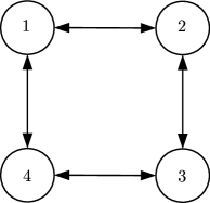
Figure 1: Interaction network.

The simulation results are illustrated in Figures 2 and 3. Figure 2 depicts the evolution of the system state. It can be seen that the variance of the system state trajectories under Algorithm 2 is much larger than those under Algorithm 4. This discrepancy arises from the direct integration of persistent noise into Algorithm 1, which sacrifices optimization accuracy and subsequently degrades the control performance of Algorithm 2. In our developed approach, the weakening factor $\chi^{k}$ is tailored to alleviate the influence of DP noise, ensuring accurate convergence of the system state. In addition, Figure 3 presents the evolution of the global constraint. It can be found that there exist constraint violations in Algorithm 2. However, owing to the implementation scheme developed in Section 4, our approach can guarantee the satisfaction of the global constraint.

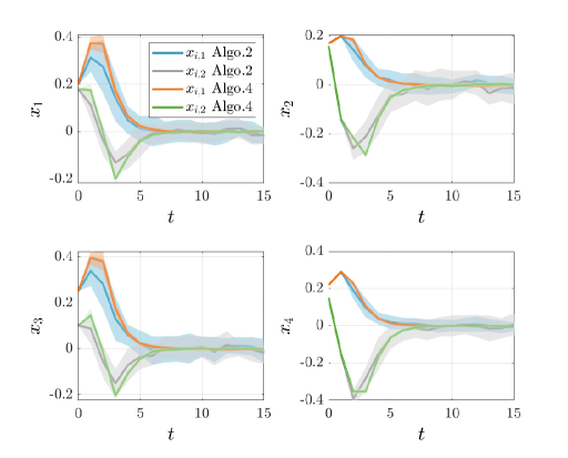
Figure 2: System state evolution.

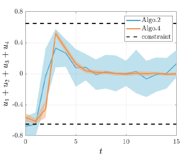
Figure 3: Global constraint evolution.

6 Conclusion

This paper developed a differentially private DMPC strategy for linear discrete-time systems with coupled global constraints. We showed that the DMPC method relying on the conventional distributed dual-gradient algorithm is susceptible to eavesdropping attacks. To address this issue, we incorporated a DP noise injection mechanism into the distributed dual-gradient algorithm, enabling privacy preservation while maintaining accurate optimization convergence. Furthermore, a practical implementation approach for DMPC was proposed, which guarantees the feasibility and stability of the closed-loop system. Simulation results validated the effectiveness of the proposed DMPC strategy.

References

• Bai et al. (2023) Bai, W., Xu, B., Liu, H., Qin, Y., Xiang, C., 2023. Robust longitudinal distributed model predictive control of connected and automated vehicles with coupled safety constraints. IEEE Transactions on Vehicular Technology 72, 2960–2973.
• Christofides et al. (2013) Christofides, P.D., Scattolini, R., de la Pena, D.M., Liu, J., 2013. Distributed model predictive control: A tutorial review and future research directions. Computers & Chemical Engineering 51, 21–41.
• Chung (1954) Chung, K.L., 1954. On a stochastic approximation method. The Annals of Mathematical Statistics , 463–483.
• Ding et al. (2021) Ding, T., Zhu, S., He, J., Chen, C., Guan, X., 2021. Differentially private distributed optimization via state and direction perturbation in multiagent systems. IEEE Transactions on Automatic Control 67, 722–737.
• Dwork et al. (2010) Dwork, C., Naor, M., Pitassi, T., Rothblum, G.N., 2010. Differential privacy under continual observation, in: Proceedings of the Forty-second ACM Symposium on Theory of Computing, pp. 715–724.
• Falsone et al. (2017) Falsone, A., Margellos, K., Garatti, S., Prandini, M., 2017. Dual decomposition for multi-agent distributed optimization with coupling constraints. Automatica 84, 149–158.
• Gade and Vaidya (2018) Gade, S., Vaidya, N.H., 2018. Private optimization on networks, in: Proceedings of the American Control Conference, IEEE. pp. 1402–1409.
• Gao et al. (2023) Gao, H., Wang, Y., Nedić, A., 2023. Dynamics based privacy preservation in decentralized optimization. Automatica 151, 110878.
• Hans et al. (2018) Hans, C.A., Braun, P., Raisch, J., Grüne, L., Reincke-Collon, C., 2018. Hierarchical distributed model predictive control of interconnected microgrids. IEEE Transactions on Sustainable Energy 10, 407–416.
• Hendrickx et al. (2015) Hendrickx, J.M., Shi, G., Johansson, K.H., 2015. Finite-time consensus using stochastic matrices with positive diagonals. IEEE Transactions on Automatic Control 60, 1070–1073.
• Huang et al. (2015) Huang, Z., Mitra, S., Vaidya, N., 2015. Differentially private distributed optimization, in: Proceedings of the 16th International Conference on Distributed Computing and Networking, pp. 1–10.
• Jin et al. (2020) Jin, B., Li, H., Yan, W., Cao, M., 2020. Distributed model predictive control and optimization for linear systems with global constraints and time-varying communication. IEEE Transactions on Automatic Control 66, 3393–3400.
• Li et al. (2021) Li, H., Jin, B., Yan, W., 2021. Distributed model predictive control for linear systems under communication noise: Algorithm, theory and implementation. Automatica 125, 109422.
• Lou et al. (2017) Lou, Y., Yu, L., Wang, S., Yi, P., 2017. Privacy preservation in distributed subgradient optimization algorithms. IEEE Transactions on Cybernetics 48, 2154–2165.
• Lu and Zhu (2018) Lu, Y., Zhu, M., 2018. Privacy preserving distributed optimization using homomorphic encryption. Automatica 96, 314–325.
• Luis et al. (2020) Luis, C.E., Vukosavljev, M., Schoellig, A.P., 2020. Online trajectory generation with distributed model predictive control for multi-robot motion planning. IEEE Robotics and Automation Letters 5, 604–611.
• Mayne (2014) Mayne, D.Q., 2014. Model predictive control: Recent developments and future promise. Automatica 50, 2967–2986.
• Michos et al. (2022) Michos, G., Baldivieso-Monasterios, P.R., Konstantopoulos, G.C., 2022. Distributed economic nonlinear mpc for DC micro-grids with inherent bounded dynamics and coupled constraints. Systems & Control Letters 167, 105327.
• Nedić et al. (2010) Nedić, A., Ozdaglar, A., Parrilo, P.A., 2010. Constrained consensus and optimization in multi-agent networks. IEEE Transactions on Automatic Control 55, 922–938.
• Notarstefano et al. (2019) Notarstefano, G., Notarnicola, I., Camisa, A., et al., 2019. Distributed optimization for smart cyber-physical networks. Foundations and Trends® in Systems and Control 7, 253–383.
• Nozari et al. (2016) Nozari, E., Tallapragada, P., Cortés, J., 2016. Differentially private distributed convex optimization via functional perturbation. IEEE Transactions on Control of Network Systems 5, 395–408.
• Olfati-Saber et al. (2007) Olfati-Saber, R., Fax, J.A., Murray, R.M., 2007. Consensus and cooperation in networked multi-agent systems. Proceedings of the IEEE 95, 215–233.
• Polyak (1987) Polyak, B.T., 1987. Introduction to optimization .
• Richards and How (2007) Richards, A., How, J.P., 2007. Robust distributed model predictive control. International Journal of Control 80, 1517–1531.
• Su et al. (2022) Su, Y., Shi, Y., Sun, C., 2022. Inexact primal-dual algorithm for DMPC with coupled constraints using contraction theory. IEEE Transactions on Cybernetics 52, 12525–12537.
• Sundaram and Hadjicostis (2007) Sundaram, S., Hadjicostis, C.N., 2007. Finite-time distributed consensus in graphs with time-invariant topologies, in: Proceedings of the American Control Conference, pp. 711–716.
• Trodden (2014) Trodden, P., 2014. Feasible parallel-update distributed MPC for uncertain linear systems sharing convex constraints. Systems & Control Letters 74, 98–107.
• Trodden and Richards (2010) Trodden, P., Richards, A., 2010. Distributed model predictive control of linear systems with persistent disturbances. International Journal of Control 83, 1653–1663.
• Wang (2019) Wang, Y., 2019. Privacy-preserving average consensus via state decomposition. IEEE Transactions on Automatic Control 64, 4711–4716.
• Wang (2023) Wang, Y., 2023. A robust dynamic average consensus algorithm that ensures both differential privacy and accurate convergence, in: Proceedings of the IEEE Conference on Decision and Control, pp. 1130–1137.
• Wang and Nedić (2024) Wang, Y., Nedić, A., 2024. Robust constrained consensus and inequality-constrained distributed optimization with guaranteed differential privacy and accurate convergence. IEEE Transactions on Automatic Control , 1–16.
• Wang and Ong (2017) Wang, Z., Ong, C.J., 2017. Distributed model predictive control of linear discrete-time systems with local and global constraints. Automatica 81, 184–195.
• Wang and Ong (2018) Wang, Z., Ong, C.J., 2018. Accelerated distributed MPC of linear discrete-time systems with coupled constraints. IEEE Transactions on Automatic Control 63, 3838–3849.
• Xiong et al. (2020) Xiong, Y., Xu, J., You, K., Liu, J., Wu, L., 2020. Privacy-preserving distributed online optimization over unbalanced digraphs via subgradient rescaling. IEEE Transactions on Control of Network Systems 7, 1366–1378.
• Zhang and Wang (2018) Zhang, C., Wang, Y., 2018. Enabling privacy-preservation in decentralized optimization. IEEE Transactions on Control of Network Systems 6, 679–689.
• Zhao et al. (2023) Zhao, D., Liu, D., Liu, L., 2023. Distributed and privacy preserving MPC with global constraints over time-varying communication. IEEE Transactions on Control of Network Systems 10, 586–598.
• Zheng et al. (2016) Zheng, Y., Li, S.E., Li, K., Borrelli, F., Hedrick, J.K., 2016. Distributed model predictive control for heterogeneous vehicle platoons under unidirectional topologies. IEEE Transactions on Control Systems Technology 25, 899–910.