Learning Diffeomorphism for Image Registration with Time-Continuous Networks using Semigroup Regularization

Abstract

Diffeomorphic image registration (DIR) is a critical task in 3D medical image analysis, aimed at finding topology preserving deformations between pairs of images. Focusing on the solution of the flow map differential equation as the diffeomorphic deformation, recent methods use discrete timesteps along with various regularization terms to penalize the negative determinant of Jacobian and impose smoothness of the solution vector field. In this paper, we propose a novel learning-based approach for diffeomorphic 3D-image registration which finds the diffeomorphisms in the time continuum with fewer regularization terms and no additional integration. As one of the fundamental properties of flow maps, we exploit the semigroup property as the only form of regularization, ensuring temporally continuous diffeomorphic flows between pairs of images. Leveraging this property, our method alleviates the need for additional regularization terms and scaling and squaring integration during both training and evaluation. To achieve time-continuous diffeomorphisms, we employ time-embedded UNets, a technique commonly utilized in diffusion models. The proposed method reveals that ensuring diffeomorphism in a continuous time interval leads to better registration results. Experimental results on two public datasets (OASIS and CANDI) demonstrate the superiority of our model over both learning-based and optimization-based methods. (https://github.com/mattkia/SGDIR/)

1 Introduction

Diffeomorphic image registration (DIR) is a computational technique used to align images into a common coordinate system using a deformation field, ensuring that the transformation is smooth and invertible [1, 2]. Unlike simpler forms of image registration that might allow folding or tearing, diffeomorphic methods preserve the topological properties of the image since the mapping between corresponding points is continuous, invertible, and differentiable. This property is significant in medical imaging, where anatomical structures need to be aligned accurately without grid folding to facilitate precise analysis and diagnosis.

Addressing the problem of diffeomorphic image registration has led to the development of various approaches, broadly categorized into traditional, optimization-based, and learning-based methods. Traditional methods such as SyN [3], NiftyReg [4], B-Splines [5], and LDDMM [6] usually start with an assumption on the model functional form and try to maximize the similarity between the moving and the fixed images while constraining the model to satisfy some regularity properties. Even though such methods can usually generate fine detailed registrations, they suffer from relatively long computation times. Recent advancements in deep neural networks have yielded optimization-based approaches using neural networks which alleviate the restriction of having an assumption on the model functional and replace the registration model with a neural network with more expressive power [7, 8, 9, 10, 11, 12]. Such models have demonstrated superior performance and lower computation times compared to traditional methods. On the other hand, learning-based approaches [13, 14, 15, 16, 17, 18, 19, 20, 21] have gained traction due to their ability to learn implicit representations of the registration process from large datasets. These methods, still leveraging deep neural network architectures can offer potentially more robust solutions, often significantly reducing computation time compared to traditional and neural optimization-based methods.

Instead of directly modeling the deformation field, most of optimization- and learning-based methods [9, 10, 19] model the velocity field controlling the dynamics of the deformation and use scaling and squaring integration scheme [22, 23] to reconstruct the deformation. Such methods typically regularize their model with various regularization terms to directly penalize the foldings in the deformation and impose smoothness on the vector field gradients and magnitudes. The advent of time-embedded architectures and time-embedded UNets [24, 25, 26] has facilitated the incorporation of the notion of time into the neural networks. Models such as DiffuseMorph [27] directly employ the Diffusion Model architecture to directly and continuously learn the deformation.

In this paper, we present a novel DIR method, called SGDIR (Semi-Group DIR), which is capable of directly generating the continuous deformation without using scaling and squaring integration and multiple regularization terms. Our method is built upon a simple yet important property of flow maps, called the semi-group property [28] which governs the composition rule of flows along time. Using time-embedded UNets our model is able to retrieve the deformation at any time step instantaneously, and hence provide a smooth transition, diffeomorphic at any time step, from the moving image to the fixed image. This is unlike the DiffuseMorph which requires to start from time zero and build up the deformation up to the given time due to following diffusion models paradigm. With a novel regularization term using the semi-group property of flow maps, we ensure diffeomorphic deformations without using any other regularization terms including penalizing negative Jacobian determinants of the deformation. Furthermore, our formulation allows us to simultaneously retrieve the reverse deformation from the fixed image to the moving image.

Our contributions can be summarized as the followings:

• We introduce a novel DIR method utilizing time-embedded UNets which is capable of producing diffeomophic deformation fields in a time continuum.

• We remove additional integration schemes such as scaling and squaring integration and regularization terms including penalization of negative Jacobian determinants of the deformation and imposition of smoothness of vector field gradient and magnitude.

• We introduce semi-group regularization as the only regularization term for leading the model to generate smooth and invertible deformations.

• We provide theoretical properties and consequences of the semi-group regularization including how it leads to temporally-continuous diffeomorphic deformations.

• We provide extensive experiments on two 3D image registration datasets which demonstrate the outperformance of SGDIR with respect to recent DIR methods.

2 Related Works

2.1 Pairwise Optimization-Based Methods

Traditional methods find the deformation field between a pair of image by minimizing an energy functional while restricting the solution space by imposing some regularity conditions on the model. SyN [6] as a successful traditional model provides a greedy technique for a symmetric diffeomorphic deformation solution by minimizing the cross-correlation between the pair of images. NiftyReg [4] as a powerful package for image registration considers different sets of linear and non-linear (such as B-Splines and Free Form Deformations (FFD)) parametric models [29] and minimizes loss functions such as Normalized Mutual Information (NMI) and Sum of Squared Differences (SSD) to maximize the alignment between the pairs of images. Traditional methods such as Demons and its variants [30, 31, 32] are built upon optical flows. LDDMM [6] is a seminal work in flow-based registration which models the registration as the geodesic paths in the images space and is proper for large deformations while preserving the topology. DARTEL [33] is also another flow-based approach which models the deformations using exponentiated Lie algebras and utilizes the scaling and squaring integration to reconstruct the deformations.

Neural optimization based approaches model the registration using neural networks. IDIR [7] and DNVF [9] are coordinate-based registration methods which utilize implicit neural representations [34]. IDIR directly learns the deformation and applies Jacobian regularization for better topology preservation and hyperelastic [35] regularization for smooth deformation, while DNVF implicitly learns the velocity field and using scaling and squaring integration reconstructs the deformation. DNVF uses Jacobian regularization along with vector field gradient and magnitude regularization. NODEO [8] which also works with voxel coordinate clouds, incorporates neural ODE networks [36] to learn the dynamics of the deformation by estimating the velocity field and finding the deformation using an ODE solver.

2.2 Learning-Based Methods

Unlike optimization-based methods which perform pairwise optimization, learning-based methods try to learn the deformation across large training datasets. The most advantageous aspect of learning-based methods is their short inference time which is orders of magnitude shorter than optimization based methods. As a fundamental work, VoxelMorph [20] directly models the deformation using a UNet and by using localized Normalized Cross Correlation metric and smoothness regularization learns the deformation fields. SYMNet [19] learns the velocity fields of forward and backward deformation and using scaling and squaring integration reconstructs the deformation. SYMNet uses Jacobian and smoothness regularizations along with minimizing the discrepancy between the forward and backward velocity fields, leading to a smoother deformation. LapIRN [37] introduces multi-resolution deformations for better generalization and avoiding local minima, and cLapIRN [16] extends LapIRN and feeds the smoothness regularization factors to the layers of the network. MS-ODE [38] incorporates neural ODEs as a refinement stage by modeling the dynamics of the parameters of a registration model.

DiffuseMorph [27] utilizes denoising diffusion models to learn temporally continuous deformations. It also incorporates Jacobian and smoothness regularization for imposing regularity on the solution. However using diffusion models could be challenging due to expensive training and maintaining visually pleasing outputs. Also, since DiffuseMorph follows the paradigm of diffusion models it requires fixed number of time samples during both training and evaluation. Furthermore, if queried at different time steps, DiffuseMorph requires to build the deformation from time step zero up to the queried time steps. Similar to DiffuseMorph we use time-embedded UNets to learn the temporally continuous deformations, but there are fundamental differences between our method and DiffuseMorph: we use a much simpler UNet without any attention modules; we are training the model with continuous time frame and we can query the model at any time step instantly. Moreover, we only use semigroup regularization introduced in this paper for learning diffeomorphic deformations.

3 Preliminaries

Deformable registration for 3D images seeks for a vector field $\phi:\mathbb{R}^{3}\longrightarrow\mathbb{R}^{3}$ which when applied to the moving image $I_{m}:\Omega\subset\mathbb{R}^{3}\longrightarrow\mathbb{R}$, deforms it smoothly towards the fixed image $I_{f}:\Omega\subset\mathbb{R}^{3}\longrightarrow\mathbb{R}$. In diffeomorphic image registration we additionally require the deformation field to be an orientation-preserving diffeomorphism, which can be mathematically translated to $\phi$ having positive determinant of Jacobian $|J_{\phi}|$ at all points. The deformation $\phi$ is usually considered to be the flow map solution of the following ordinary differential equation [39, 40, 6, 33, 19]:

$$\left\{\begin{array}[]{ll}\frac{d\phi}{dt}=\mathbf{V}(\phi)&\\ \phi_{0}(x)=x,&\\ \end{array}\right.$$ (3)

where $\phi_{0}(x)$ is short for $\phi(x,t=0)$ and $\mathbf{V}:\mathbb{R}^{3}\longrightarrow\mathbb{R}^{3}$ is a stationary velocity field governing the dynamics of the flow. In the context of DIR, $\phi_{1}(x)$ is taken to be the deformation which warps $I_{m}$ to $I_{f}$. The utility of the ODE of Eq.(3) is that its solution is guaranteed to be a diffeomorphism. It is shown that considering

$$\phi_{\frac{1}{2^{N}}}(x)=x+\frac{\mathbf{V}}{2^{N}}$$ (4)

for a relatively large $N$ (e.g., $N=8$) allows one to use the scaling and squaring integration scheme to find $\phi_{1}(x)$ by iteratively applying the deformations [22, 23]:

$$\phi_{1/2^{N-1}}=\phi_{1/2^{N}}\circ\phi_{1/2^{N}}\Rightarrow\phi_{1/2^{N-2}}=\phi_{1/2^{N-1}}\circ\phi_{1/2^{N-1}}\Rightarrow\dots\Rightarrow\phi_{1}=\phi_{1/2}\circ\phi_{1/2}.$$ (5)

Conventional DIR methods, taking advantage of the above properties, assume the following general loss function to address the diffeomorphic registration problem

$$\mathcal{L}=\mathbb{E}_{(I,J)\sim\mathcal{D}}\left[\mathcal{L}_{\text{sim}}(I,\phi[J])+\mathcal{L}_{\text{reg}}(\phi)\right],$$ (6)

where $\mathcal{D}$ is the distribution of the images, $\mathcal{L}_{\text{sim}}(.,.)$ is a measure of similarity between the fixed image and the warped moving image, and $\mathcal{L}_{\text{reg}}(\phi)$ contains restrictive regularization terms over the deformation $\phi$. Here, $\phi[J]$ means the warping of image $J$ under the deformation field $\phi$. Starting with an estimation of the vector field $\mathbf{V}$ in Eq.(4), the deformation $\phi$ (more precisely, $\phi_{1}$) is obtained by scaling and squaring integration, and the whole model is optimized to minimize the loss Eq. (6).

On the other hand, a necessary and sufficient condition of $\phi$ as the flow map solution of the ODE of Eq.(3) is that it satisfies the semigroup property; i.e., for any time steps $t$ and $s$ it holds [41]:

$$\phi(\phi(x,s),t)=\phi(\phi(x,t),s)=\phi(x,s+t),$$ (7)

or in short

$$\phi_{t}\circ\phi_{s}=\phi_{s}\circ\phi_{t}=\phi_{t+s}.$$ (8)

Intuitively, this means that deforming an image $I$ up to a time $t+s$ is equivalent to first deforming the image up to time $t$ to obtain $I_{t}$, and then applying the deformation again up to time $s$ given that the initial condition has changed to $I_{t}$. Also, since $\phi_{t}\circ\phi_{-t}(x)=\phi_{0}(x)=x$, we can easily deduce that

$$\phi^{-1}_{t}(x)=\phi_{-t}(x),$$ (9)

for all values of $x$. Given that $\phi$ is a differentiable function, Eq. (9) guaranties the bijectivity of $\phi_{t}(x)$. In the next section we’ll show how we exploit the semigroup property of Eq.(8) to circumvent the scaling and squaring integration and other regularization terms and perform the registration in a continuous time frame in contrast to former DIR methods which find the deformation at time $1$.

4 Proposed Method

Here we elaborate our method, dubbed as SGDIR. Let $I_{f},I_{m}:\Omega\longrightarrow\mathbb{R}$ be the fixed and moving images, respectively, sampled from the images distribution $\mathcal{D}$. Here, $\Omega\subset\mathbb{R}^{3}$ is a cubical region of size $D\times H\times W$. We are looking for a time-continuous deformation field $\phi:\Omega\times\mathbb{R}\longrightarrow\mathbb{R}^{3}$ to deform the moving image towards the fixed image, and vice versa. We assume that $\phi$ is the flow map solution of the ODE 3, for some unknown stationary vector field $\mathbf{V}$, and therefore, it must satisfy the semigroup property of Eq.(8). If we warp $I_{m}$ up to time $t$ using the deformation $\phi_{t}$, and warp $I_{f}$ up to time $1-t$ using the inverse deformation $\phi^{-1}_{1-t}$, we must reach to a same point due to the continuity of the trajectory of $\phi$. Based on Eq.(9) on the inversion of $\phi$, we can write

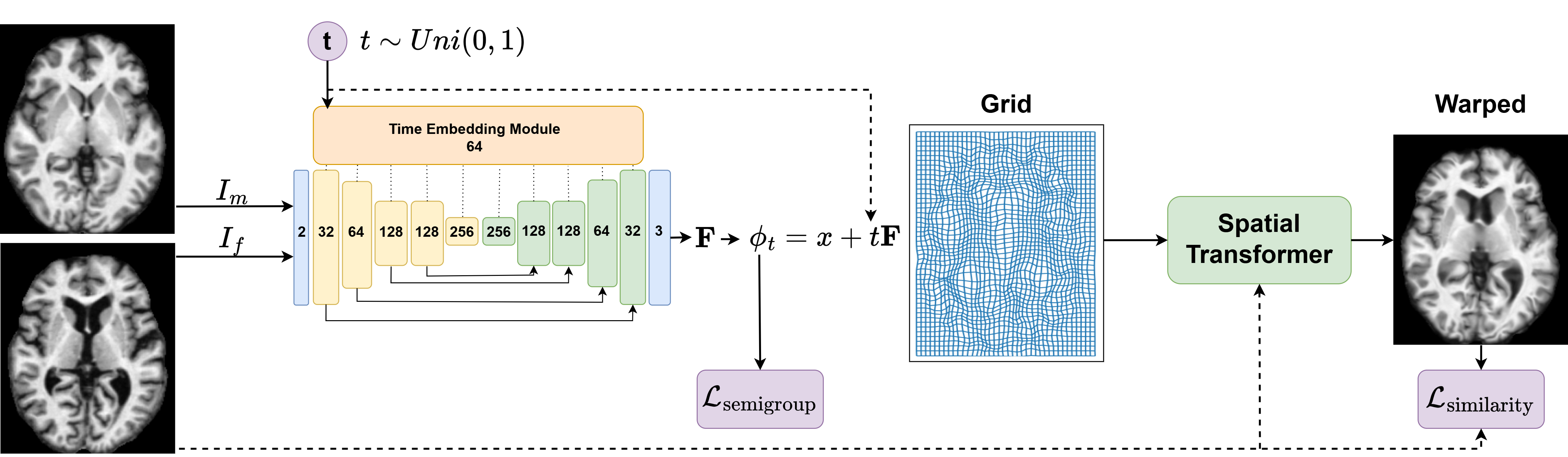
Figure 1: The general schematic of the SGDIR. As illustrated in the figure, there are no additional integration or extra loss functions applied which makes the whole procedure simpler.

$$\phi^{-1}_{1-t}[I_{f}]=\phi_{t-1}[I_{f}]=\phi_{t}[I_{m}].$$ (10)

Eq.(10) allows us to define time-continuous similarity loss. For measuring the similarity, we use the localized Normalized Cross Correlation (NCC) between the images [20, 8] (A.1). In this work we use a local window of size $11$ in NCC. Using Eq.(10), we introduce a time-continuous similarity loss:

$$\mathcal{L}_{\text{sim}}(t) =-NCC(\phi_{t-1}[I],\phi_{t}[J]), ~{}\forall t\in[0,1].$$ (11)

We propose to learn the time-continuous deformation $\phi(x,t)$ using a time-embedded UNet as shown in Figure 1. The Time-Embedded UNet (TE-UNet), frequently used in diffusion models, is capable of incorporating the notion of time and is suitable for learning flow maps. To achieve this goal, we model the deformation $\phi$ as

$$\phi_{t}(x;\theta)=\phi(x,t;\theta)=x+t\mathbf{F}(x,t;I,J,\theta),~{}\forall t\in[-1,1],$$ (12)

where $\mathbf{F}(x,t;I,J,\theta)$ is a TE-UNet with learnable parameters $\theta$ which also receives the pair of fixed and moving images. The reason behind the specific formulation of Eq.(12) is that we can make sure that at $t=0$ we have $\phi_{0}(x)=x$, hence satisfying the identity initial condition of the ODE 3. In order for $\phi$ to be a valid flow map, it needs to satisfy the semigroup property of Eq. (8). In practice, forcing the model to perfectly satisfy the semigroup property could be cumbersome and expensive, since we need to sample $t$ and $s$ independently and impose Eq. (11) twice, which requires more forward calls from the network. To tackle this issue we propose the following regularization,

$$\mathcal{L}_{\text{reg}}(t)=\|\phi_{2t-1}-\phi_{t}\circ\phi_{t-1}\|_{2}+\|\phi_{2t-1}-\phi_{t-1}\circ\phi_{t}\|_{2},~{}\forall t\in[0,1],$$ (13)

and we show that it suffices to render $\phi$ invertible and consequently a diffeomorphism at all time steps $t\in[-1,1]$. In Eq. (13), $\|.\|_{2}$ denotes the $L_{2}$-norm, and forces the model to satisfy the semigroup property for $t$ and $s=t-1$. The second term in Eq. (13) is added only to impose symmetry and provide diffeomorphism in $[-1,0]$ interval. Similar to all DIR methods we implement the composition operation by trilinear interpolation of grids over each other [19, 9, 37, 16]. From Eq. (13), one could instantly say that a model that minimizes Eq. (13), will satisfy the following rules

$$\phi_{2t-1}=\phi_{t}\circ\phi_{t-1},~{}\phi_{2t-1}=\phi_{t-1}\circ\phi_{t}.$$ (14)

Proposition 1.

The deformation $\phi(x,t)$ optimally learned by minimizing Eq. (11) and Eq. (13), is a diffeomorphism at any time $t\in[-1,1]$.

Proof.

See Appendix A.2. ∎

Finally, we can propose the following loss function which is in concordance with Eq. (6):

$$\mathcal{L}=\mathbb{E}_{(I_{f},I_{m})\sim\mathcal{D},t\sim Uni(0,1)}\left[\mathcal{L}_{\text{sim}}(t)+\lambda\mathcal{L}_{\text{reg}}(t)\right],$$ (15)

where $Uni(0,1)$ is the uniform distribution on $[0,1]$ and $\mathcal{L}_{\text{sim}}$ and $\mathcal{L}_{\text{reg}}$ are defined as in Eq. (11) and Eq. (13), respectively. $\lambda$ is the regularization factor controlling the level of diffeomorphism. In the training phase, we randomly sample a pair of images to be registered along with a time step uniformly taken from the interval $[0,1]$ to minimize Eq. (15). The trained model is capable of warping either $I_{f}$ or $I_{m}$ towards each other at any time step. Thus, the model is more versatile compared to the most previous works that provide the deformation in only one direction.

5 Experiments

5.1 Datasets and Preprocessing

To evaluate SGDIR and compare its performance with other methods, we consider two publicly available datasets on 3D MR brain scans widely used in the literature, namely Open Access Series of Image Studies (OASIS) [42] and the Child and Adolescent NeuroDevelopment Initiative (CANDI) [43]. OASIS dataset contains 416 T1 weighted scans from subjects aging from 18 to 96 with 100 of them diagnosed with mild to moderate Alzheimer’s disease. The segmentation masks of 35 subcortical regions available in the dataset serve as the ground truth for further evaluation of the registration. CANDI dataset contains T1 weighted brain scans of 117 subjects divided into 4 different subgroups including Healthy Control (HC), Schizophrenia Spectrum (SS), Bipolar Disorder with Psychosis (BPDwithPsy), and Bipolar Disorder without Psychosis (BPDwithoutPsy). The segmentation masks of 32 subcortical regions available in the dataset are used as the ground truth for the evaluation. For both datasets we use the skull stripped, MNI152 1mm normalized images and center-crop the images to the size $160\times 192\times 144$. For both datasets we use all the available anatomical structures for evaluation. We also use min-max intensity normalization to transform the voxel intensities into the $[0,1]$ range. In the training phase, in order for the arguments of Proposition 1 remain valid we add a slight standard Gaussian noise with 0 mean and 0.01 standard deviation to the data. This makes sure that no pairs of voxels have precisely the same intensity levels while the image pair remaining visually intact.

5.2 Experimental Settings

In the OASIS dataset we use the first 256 subjects for training the model, the next 50 subjects for the validation and the rest of the subjects for the test set. By random sampling we generate 900 pairs for training, 100 pairs for validation and 225 pairs for test. In the CANDI dataset, we mix all the subgroups and then use 80 subjects for training, 11 subjects for validation, and the rest for the test set. In a similar way to the OASIS dataset, we generate 400 pairs for training, 25 pairs for validation, and 100 pairs for test. We compare the performance of our model in terms of Dice score and the percentage of negative determinants of Jacobian of the deformation, with a traditional optimization-based method, SyN [3], as one of the most successful methods for diffeomorphic image registration, learning-based methods including SYMNet [19], VoxelMorph [20], and DiffuseMorph [27], and optimization-based methods such as IDIR [7], NODEO [8], DNVF and its variant Cas-DNVF [9]. For SyN, we used the implementation in the DIPY package [44] and used cross-correlation for the loss function following the convention of the VoxelMorph. For other methods, except for DNVF/Cas-DNVF whose implementation was not available at the time of writing this paper, we used the codes available in their corresponding official repositories. The architecture of the UNet along with the time embedding modules is shown in Figure 1. The UNet encoder has 5 down-sampling layers of dimensions 32, 64, 128, 128, and 256, and the decoder has 5 up-sampling layers with the same dimensions as the down-sampling layers but in the reversed order. The time-embedding dimension is set to 64. All the activation functions for the layers are set to SiLU [45] to provide more smoothness to the network. In our experiments the regularization factor for the semigroup term is set to $\lambda=5e^{5}$, the NCC window size is set to 11, and the training is carried out for 100 epochs using Adam optimizer with the learning rate $lr=1e^{-4}$. The whole implementation is done in PyTorch and is tested on both NVIDIA GTX 1080 Ti and NVIDIA Tesla V100 GPUs with 32Gb RAM.

5.3 Evaluation Metrics

A successful DIR model, deforms the moving image towards the fixed image such that the moving image becomes as structurally similar as possible to the fixed image while the topology of the moving image is not disrupted. Following the convention of evaluating the diffemorphic image registration methods ([9, 8, 19, 37]), we use Dice Similarity Coefficient to measure the similarity of the registered image and the target image, and we use the negative Jacobian determinant percentage to measure the amount of disturbance in the topology of the moving image.

5.3.1 Dice Similarity Coefficient

Dice similarity coefficient is a method to measure the amount of overlap between the registered image and the target image. For our experiments we use the segmentation masks (with 35 and 32 structures for the OASIS and CANDI datasets, respectively) of the deformed image and the fixed image to measure the Dice coefficient. We follow the convention of VoxelMorph [20] for computing the Dice score, which measures the mean Dice over all anatomical structures.

5.3.2 Negative Jacobian Determinant Percentage

The Jacobian determinant of the deformation (here and after denoted by $|det(J_{\phi})<0|$) at each point determines if the deformation is a local diffeomorphism (according to the Inverse Function Theorem) [19]. Having positive Jacobian determinant at any point means an orientation preserving diffeomorphism at that point. Therefore, the percentage of the voxels at which the deformation exhibits non-positive Jacobian determinant is a measure of how well the model is preserving the topology. A lower the percentage of non-positive Jacobian determinant is an indication of better preservation of the topology and avoiding folding in the grid.

Table 1: Comparison of the performance of SGDIR with other methods. The values inside the parenthesis indicate the standard deviation. Cells with - indicate that the corresponding information is missing in the literature. $\approx 0$ sign is used for negative determinant percentages smaller than an order of $10^{-5}$.

		OASIS		CANDI
Category	Model	Dice ($\uparrow$)	$|\text{det}(J_{\phi})<0|$ ($\downarrow$)	Dice ($\uparrow$)	$|\text{det}(J_{\phi})<0|$ ($\downarrow$)
Traditional	SyN	78.14 (1.32)	0.0531% (0.0241)	73.60 (1.15)	0.0011% (0.0008)
Learning	VoxelMorph	75.93 (0.044)	0.0026% (0.0027)	75.63 (1.78)	0.0011% (0.0010)
	SYMNet	79.39 (1.74)	0.0043% (0.0017)	75.89 (1.13)	0.0015% (0.0013)
	DiffuseMorph	76.23 (2.23)	0.0551% (0.0431)	75.63 (2.01)	0.0041% (0.0012)
Optimization	IDIR	72.31 (1.239)	0.0389% (0.0025)	74.42 (1.12)	0.0113% (0.0081)
	NODEO	80.86 (1.14)	0.0105% (0.0115)	78.02 (1.52)	$\approx$ 0%
	DNVF	79.4	0.0015%	78.6	0.0003%
	Cas-DNVF	81.5	0.0036%	-	-
Our Method	SGDIR	82.23 (1.3851)	0.0009% (0.0007)	80.73 (1.25)	$\mathbf{\approx 0}$%

Figure 2: Qualitative comparison of SGDIR with learning-based and optimization-based methods including SYMNet, VoxelMorph, NODEO, IDIR, and DiffuseMorph on the OASIS dataset.

5.4 Results

Table 1 provides a comprehensive comparison of the performance of SGDIR with other aforementioned traditional, learning-based, and optimization-based methods. This table provides the performance of models in terms of Dice score and the percentage of negative Jacobian determinants. All the values are expressed as their average over the test set along with their standard deviation. For DNVF and Cas-DNVF due to unavailability of the implementation the results are directly taken from the corresponding paper, and the missing information is shown with - in the table. We consider the percentage of negative Jacobian determinants smaller than $10^{-5}$ negligible and show it as $\approx 0$ in the table. Also, Figure 2 illustrates the qualitative comparison between our model and several other models in terms of the warped image, warped segmentations, and the warping grids.

Table 1 indicates that SGDIR outperforms competent methods both in terms of Dice score, and $|det(J_{\phi})<0|$ implying that the imposition of the semigroup property as a regularization in the time continuum of the deformation field can in fact lead to a smooth deformation.

Among the compared methods, DiffuseMorph is also capable of generating a deformation flow. Therefore, we have provided a visual comparison of warped images within 7 time steps for the OASIS dataset in Figure 3. In this example we have used the subject id 1 and 2 of the OASIS dataset as the fixed image and the moving image respectively. More visual results are also provided in Appendix B.

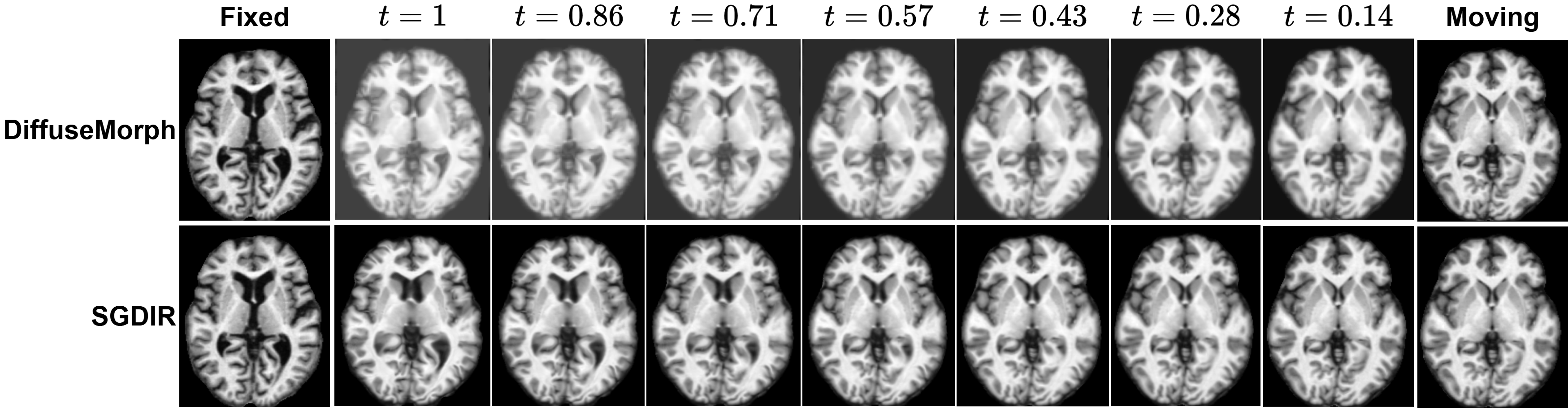
Figure 3: The visual comparison of the continuous deformations of DiffuseMorph and SGDIR for OASIS dataset.

5.5 Ablation Study

In addition to the main results on the efficacy of SGDIR in providing high Dice scores while maintaining low $|det(J_{\phi})<0|$, we investigate the effect of some hyperparameters and design choices along with some consequent properties of SGDIR. More precisely, we investigate the effect of the semigroup regularization factor $\lambda$, the effect of continuous time scale against discrete time, and the topology-preserving property throughout the time interval. Since the behaviour of the model is the same for both OASIS and CANDI dataset, we provide the analysis only for the OASIS dataset which is a more complex dataset with larger deformations.

5.5.1 Effect of Regularization Factor

Eq. (13) is responsible to impose the semigroup property to the model and consequently, make the model produce topology-preserving non-folding deformations. Table 2 provides the effect of changing the factor $\lambda$ for the semigroup regularization on the Dice score and $|det(J_{\phi})<0|$. This table indicates that for a choice of a very large $\lambda$ we could achieve zero-folding deformations with a decrease in the dice score. Decreasing $\lambda$ gives more freedom to the model to increase the similarity of the deformed image and the fixed image in exchange for a larger folding percentage. An interesting property exhibited here is that drastically decreasing $\lambda$ (e.g., $\lambda=1$) is not helpful for achieving the highest Dice score. This indicates that the semigroup property is also helpful in narrowing down the trajectory space of the deformations, helping the model to converge to the more optimal solution.

Table 2: Analysis of the effect of the semigroup regularization factor on the Dice score and the percentage of negative Jacobian determinants over the OASIS dataset.

	Performance
$\lambda$	Dice $(\uparrow)$	$|\text{det}(J_{\phi})<0|$ $(\downarrow)$
$10^{7}$	76.20	0.0000%
$10^{5}$	82.11	0.0011%
$10^{4}$	83.45	3.0691%
$10^{3}$	82.66	6.0955%
$10^{2}$	80.01	6.7403%
$10$	80.23	7.0794%
$1$	79.80	7.8612%

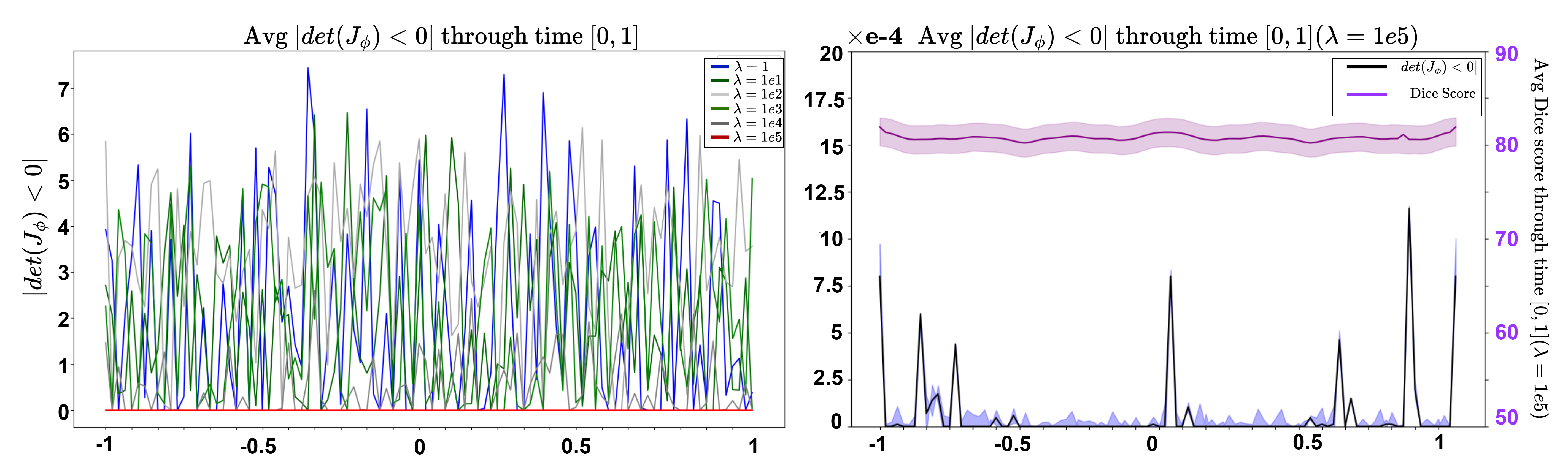
Figure 4: The percentage of negative Jacobian determinants through time. The left figure compares the effect of $\lambda$ on the $|det(J_{\phi})<0|$ and the right figure focuses on the best configuration model. The shaded area in the right figure indicates the variance across the test set. The negative time scale indicates the interval which warped the fixed image towards the moving image (reverse warping).

5.5.2 Diffeomorphism Through Time

Applying the semigroup regularization ensures that the deformation is a diffeomorphism not only at the endpoints, but also at all times $t\in[0,1]$. Figure 4 illustrates how $|det(J_{\phi})|$ varies across time. The negative time interval is used for reverse warping; i.e., warping the fixed image towards the moving image. The left figure illustrates the effect of different values of $\lambda$ on $|det(J_{\phi})<0|$ throughout the time interval, and one can see that a proper factor for the semigroup regularization could lead to an almost perfect diffeomorphism in each time step. The right figure, focuses on the performance of the best model. The purple plot and the right y-axis indicate the Dice score of intermediate warped images throughout time and the black plot and the left y-axis indicate the $|det(J_{\phi})<0|$. The shaded areas for both plots show the variance of the corresponding metric. We observe that the semigroup regularization successfully preserves the topology at all time steps, while keeping the Dice score high during the transition.

5.5.3 Effect of Discrete Time Steps

SGDIR can retrieve the deformation at an arbitrary time step using a continuous sampling from the time interval $[0,1]$. Here, we investigate the effect of using discrete time steps for training the model. At the evaluation phase, we query the model at times 1 and -1 to warp the moving image towards the fixed image, and warp the fixed image towards the moving image, respectively. Table 3 demonstrates that increasing the number of time samples in the interval $[0,1]$ improves the performance of the model both in terms of Dice score and $|det(J_{\phi})<0|$, while the best performance is achieved by continuous sampling. Figure 5 in Appendix B provides an illustrative inspection of this effect as well.

Table 3: Analysis of the effect of using discrete time steps on the Dice score and the percentage of negative Jacobian determinants. The number of time steps indicate the number of intermediate time steps used. For instance, 0 time steps means that only the endpoint are used for registration (at time 1), and 8 time steps means that 8 intermediate time steps is used. $\infty$ is the continuous time sampling as done in our method.

	Performance
# Time Steps	Dice	$|\text{det}(J_{\phi})<0|$
$0$	73.12	13.121%
$1$	73.68	0.152%
$2$	74.23	0.065%
$4$	75.03	0.008%
$8$	75.45	0.002%
$\infty$	82.23	0.0009%

6 Conclusion

In this paper, we proposed SGDIR, a novel learning-based model for image registration based on time-embedded UNet architecture and using semigroup-based regularization. The time-embedded network allows us to retrieve the deformation and consequently warping at any time step and the semigroup regularization enables the model to generate diffeomorphic deformations at any time step. The resulting model is capable of generating smooth warpings from the moving image to the fixed image and vice versa without requiring any integration scheme and using further regularization terms on the smoothness of the deformation. We evaluated our model on two benchmark datasets on 3D medical image registration and demonstrated superiority in various metrics compared to state-of-the-art optimization- and learning-based methods. In a broader perspective, the proposed framework in this paper provides a systematic method for addressing problems which can be modeled as autonomous ODEs.

Appendix A Appendix / supplemental material

A.1 Definition of the NCC loss function

The NCC loss function used in this paper is similar to the definition used by previous methods [20, 19, 8, 9]. For a pair of images $I$ and $J$ the localized NCC is defined as

$$NCC(I,J)=\sum_{W_{p},p\in\Omega}\frac{\left(\sum_{p_{i}\in W_{p}}(I(p_{i})-\mu_{I_{W_{p}}}(p_{i}))(J(p_{i})-\mu_{J_{W_{p}}}(p_{i}))\right)^{2}}{\sum_{p_{i}\in W_{p}}(I(p_{i})-\mu_{I_{W_{p}}}(p_{i}))^{2}\sum_{p_{i}\in W_{p}}(J(p_{i})-\mu_{J_{W_{p}}}(p_{i}))^{2}},$$ (16)

where $\Omega$ is the definition domain of images and $W_{p}$ is a local window around the point $p\in\Omega$. The terms $I(p_{i})$ and $J(p_{i})$ denote the value of image $I$ and $J$ at the point $p_{i}$, respectively. Also, $\mu_{I_{W_{p}}}$ and $\mu_{J_{W_{p}}}$ denote the mean intensity of $I$ and $J$ in the local window $W_{p}$, respectively. The highest value for NCC is 1 in the case that $I$ and $J$ perfectly match, and the lowest value is 0 for the case of no correspondence.

A.2 Proofs

In order to prove Proposition 1, we present the following short lemma, and then proceed to proving the proposition.

Lemma 1.

The model minimizing Eq. (11), will optimally satisfy the following rules for any $t\in[0,1]$:

$$\phi_{t-1} =\phi_{t}\circ\phi_{-1}$$

$$\phi_{t} =\phi_{t-1}\circ\phi_{1}.$$ (17)

Proof.

In the optimal case, the deformation $\phi$ deforms $I_{m}$ towards $I_{f}$, at any time step $t$, perfectly. Thus, we can write

$$\phi_{t}[I_{m}]=\phi_{t-1}[I_{f}].$$ (18)

Setting $t=0$, we get $\phi_{0}[I_{m}]=I_{m}=\phi_{-1}[I_{f}]$ due to the identity condition at $t=0$. We substitute $I_{m}$ with $\phi_{-1}[I_{f}]$ in Eq. (18), and obtain

$$\phi_{t}[\phi_{-1}[I_{f}]]=\phi_{t}\circ\phi_{-1}[I_{f}]=\phi_{t-1}[I_{f}].$$ (19)

Assuming that $I_{f}$ contains points with unique values, we can conclude that

$$\phi_{t-1}=\phi_{t}\circ\phi_{-1}.$$ (20)

Similarly, by setting $t=1$, we get $I_{f}=\phi_{1}[I_{m}]$, and following the same procedure we will get

$$\phi_{t}=\phi_{t-1}\circ\phi_{1}.$$ (21)

∎

Remark 1.

The assumption made in proving Lemma 1 regarding the unique intensities for the voxels of an image usually does not hold. However, in practice, we add a small Gaussian noise to the image to make the assumption valid. Adding the Gaussian noise makes the probability of two voxels having the same intensity zero, and we verified this in our experiments as well.

Corollary 1.

$\phi_{1}$ and $\phi_{-1}$ are inverse of each other.

Proof.

Using the result from Lemma 1, and evaluating Eq. (20) at $t=1$, we get $\phi_{1}\circ\phi_{-1}(x)=\phi_{0}(x)=x$. Similarly, evaluating Eq. (21) at $t=0$ gives us $\phi_{-1}\circ\phi_{1}(x)=\phi_{0}(x)=x$. Therefore, $\phi_{1}$ and $\phi_{-1}$ are inverse of each other ∎

Proposition 1. The deformation $\phi(x,t)$ optimally learned by minimizing Eq. (11) and Eq. (13), is a diffeomorphism at any time $t\in[-1,1]$.

Proof.

From Corollary 1, we get that $\phi_{1}$ is diffeomorphism. Also, by definition, $\phi_{0}$ is the identity function and is therefore, a diffeomorphism. Take an arbitrary $s\in[0,1]$, and consider the rules $\phi_{2t-1}=\phi_{t}\circ\phi_{t-1}$ from Eq. (14), and $\phi_{t-1}=\phi_{t}\circ\phi_{-1}$ from Eq. (20) for $t\in[0,1]$. Then we can write

$$\phi_{2t-1}=\phi_{t}\circ\phi_{t-1}=\phi_{t}\circ\phi_{t}\circ\phi_{-1}.$$

Letting $2t=s$, we get for $s\in[0,2]$

$$\phi_{s-1}=\phi_{s/2}\circ\phi_{s/2}\circ\phi_{-1}.$$

So it is also true for $s\in[0,1]$. Now, composing both sides of the equation with $\phi_{1}$ from right, we get

$$\phi_{s-1}\circ\phi_{1}=\phi_{s/2}\circ\phi_{s/2}\circ\phi_{-1}\circ\phi_{1}.$$

Knowing that $\phi_{s-1}\circ\phi_{1}=\phi_{s}$ and $\phi_{-1}\circ\phi_{1}=Id$, we get

$$\phi_{s}=\phi_{s/2}\circ\phi_{s/2},~{}\forall s\in[0,1].$$ (22)

Eq. (22) is the familiar form of the scaling and squaring integration scheme. Iterative compositions of $\phi_{s/2}$ terms can arbitrarily get close to $\phi_{0}$. Since $\phi_{t}$ is locally a diffeomorphism at $t=0$ and we can get arbitrarily close to $\phi_{0}=Id$ , according to [22], the scaling and squaring composition of Eq (22) will lead to a diffeomorphism. Therefore, $\phi_{s},s\in[0,1]$ is a diffeomorphism.

Similarly, by taking the rules $\phi_{2t-1}=\phi_{t-1}\circ\phi_{t}$ from Eq. (14), and $\phi_{t}=\phi_{t-1}\circ\phi_{1}$, we get

$$\phi_{2t-1}=\phi_{t-1}\circ\phi_{t}=\phi_{t-1}\circ\phi_{t-1}\circ\phi_{1}.$$

By substituting $t-1$ with $-u$, we get for $u\in[0,1]$

$$\phi_{-2u+1}=\phi_{-u}\circ\phi_{-u}\circ\phi_{1}.$$

Substituting $2u$ with $s$, we get for $s\in[0,2]$

$$\phi_{1-s}=\phi_{-s/2}\circ\phi_{-s/2}\circ\phi_{1}.$$

Thus it is also true for $s\in[0,1].$ Now using $\phi_{1-s}=\phi_{1-s-1}\circ\phi_{1}=\phi_{-s}\circ\phi_{1}$ and composing both sides with $\phi_{-1}$ from right, we get

$$\phi_{-s}=\phi_{-s/2}\circ\phi_{-s/2},~{}\forall s\in[0,1].$$ (23)

Thus, we have the same scaling and squaring scheme in the $[-1,0]$ interval. So, we conclude that $\phi_{t}$ is a diffeomorphism over $[-1,1]$ interval. ∎

Appendix B More Visual Results

Figure 5 illustrates the evaluation of SGDIR for various number of sampled time steps for the subject ids 1 and 2 of the OASIS dataset. In this figure, both forward and backward deformations along with their warped images are illustrated.

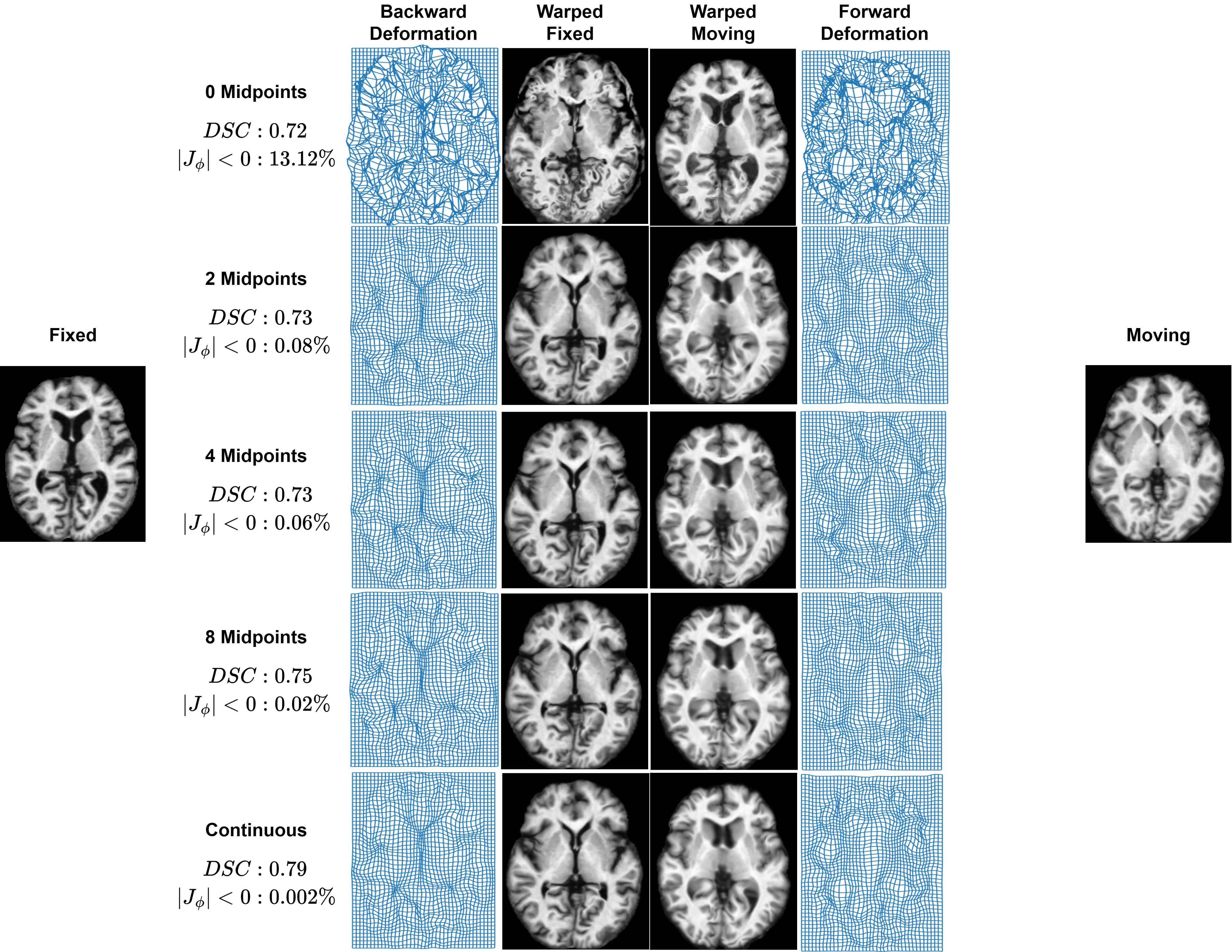
Figure 5: The effect of number of intermediate time steps on the smoothness (percentage of negative Jacobian determinants) and the Dice score.

Figure 6 illustrates more warping examples on the OASIS dataset. This figure contains the result of registrations of both small and large deformations.

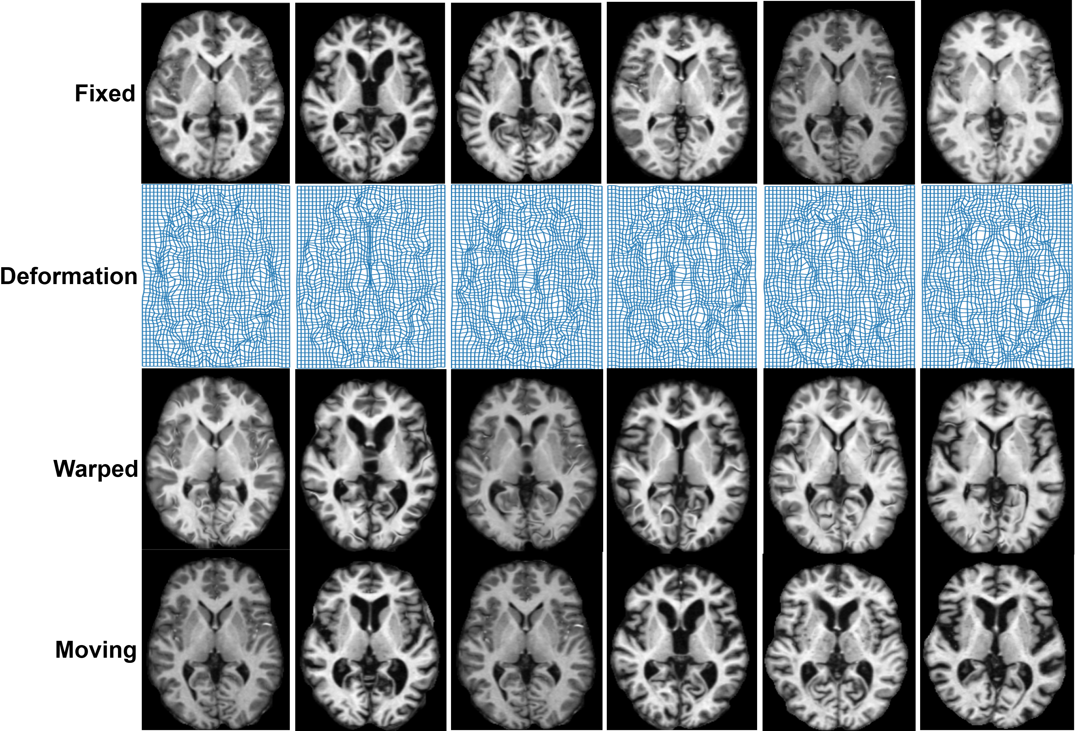
Figure 6: Visual performance of SGDIR on samples from OASIS dataset containing both small and large deformation. The first and last rows show the fixed and moving images, respectively. The second row depicts the deformation grid output by SGDIR and the third row shows the result of registration.

Figure 7 illustrates warping examples on the CANDI dataset. Since CANDI dataset contains pairs with smaller deformations, the deformation grids are depicted in full resolution to better reflect the deformations.

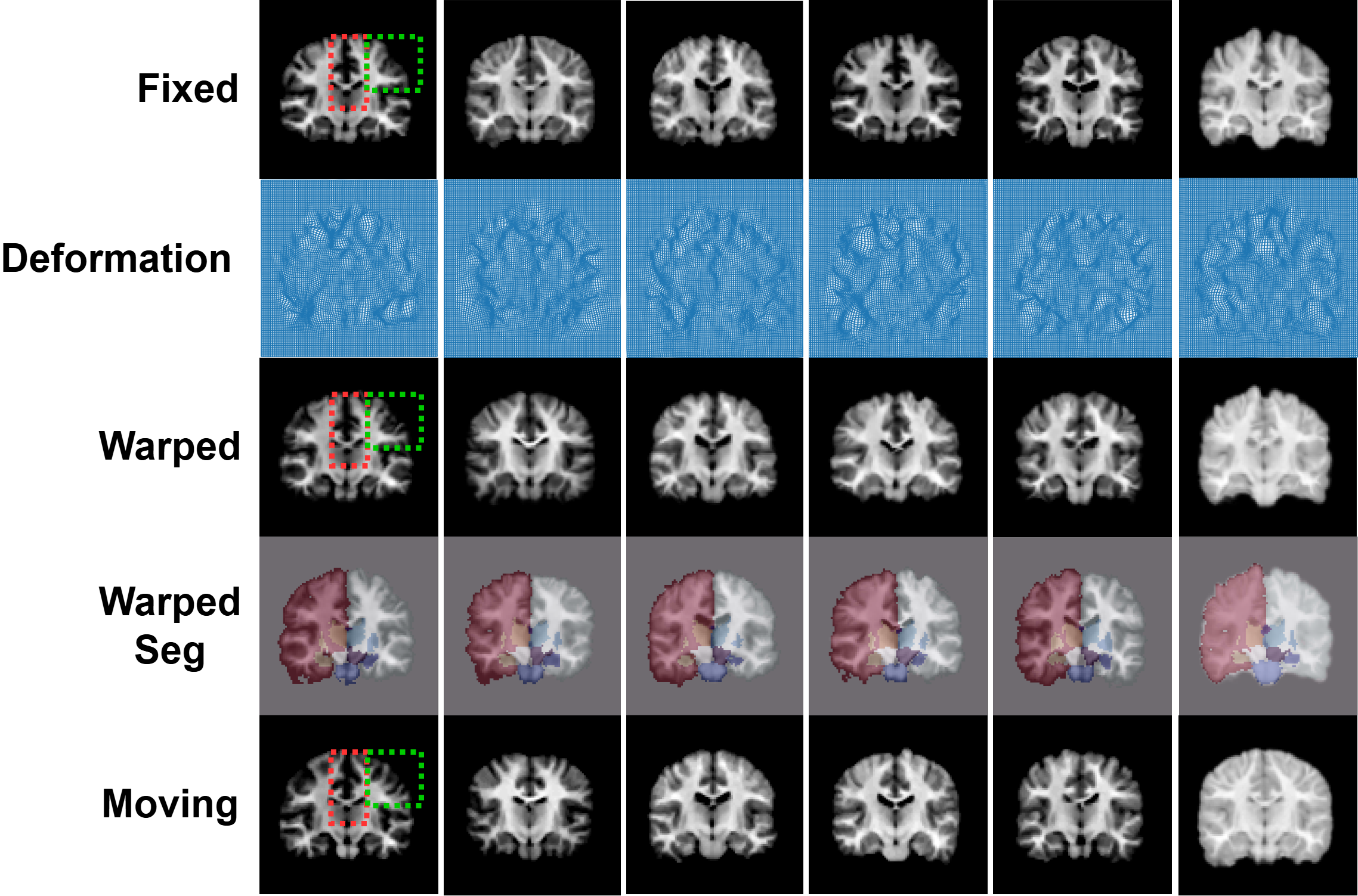
Figure 7: Visual performance of SGDIR on samples from CANDI dataset. The first and last rows show the fixed and moving images, respectively. The second row depicts the deformation grid output by SGDIR, the third row shows the result of registration, and the fourth row shows the warping of the segmentation mask.

Figure 8 illustrates the visual comparison of the performance of our model (SGDIR) with respect to other models on the CANDI dataset.

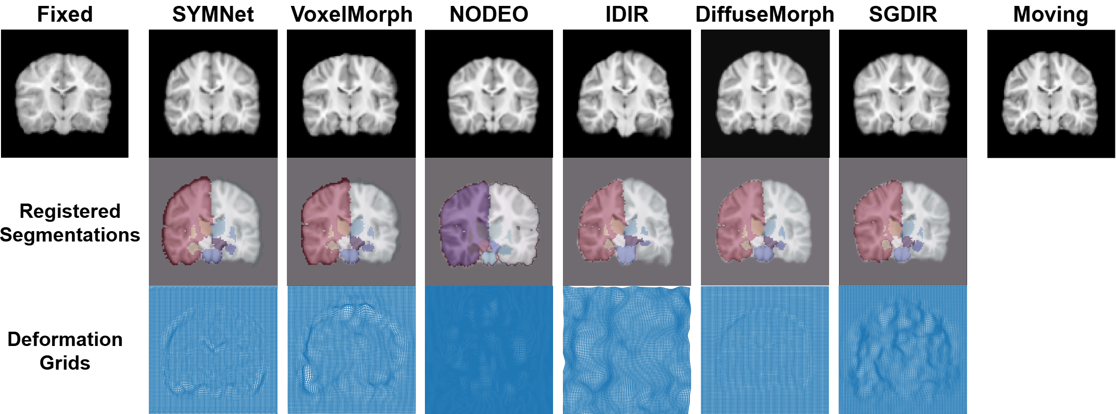
Figure 8: Qualitative comparison of SGDIR with learning-based and optimization-based methods including SYMNet, VoxelMorph, NODEO, IDIR, and DiffuseMorph over the CANDI dataset.

References

- [1] Aristeidis Sotiras, Christos Davatzikos, and Nikos Paragios. Deformable medical image registration: A survey. IEEE transactions on medical imaging, 32(7):1153–1190, 2013.
- [2] Nicholas J Tustison, Brian B Avants, and James C Gee. Learning image-based spatial transformations via convolutional neural networks: A review. Magnetic resonance imaging, 64:142–153, 2019.
- [3] Brian B Avants, Charles L Epstein, Murray Grossman, and James C Gee. Symmetric diffeomorphic image registration with cross-correlation: evaluating automated labeling of elderly and neurodegenerative brain. Medical image analysis, 12(1):26–41, 2008.
- [4] Marc Modat, Gerard R Ridgway, Zeike A Taylor, Manja Lehmann, Josephine Barnes, David J Hawkes, Nick C Fox, and Sébastien Ourselin. Fast free-form deformation using graphics processing units. Computer methods and programs in biomedicine, 98(3):278–284, 2010.
- [5] Daniel Rueckert, Luke I Sonoda, Carmel Hayes, Derek LG Hill, Martin O Leach, and David J Hawkes. Nonrigid registration using free-form deformations: application to breast mr images. IEEE transactions on medical imaging, 18(8):712–721, 1999.
- [6] M Faisal Beg, Michael I Miller, Alain Trouvé, and Laurent Younes. Computing large deformation metric mappings via geodesic flows of diffeomorphisms. International journal of computer vision, 61:139–157, 2005.
- [7] Jelmer M Wolterink, Jesse C Zwienenberg, and Christoph Brune. Implicit neural representations for deformable image registration. In International Conference on Medical Imaging with Deep Learning, pages 1349–1359. PMLR, 2022.
- [8] Yifan Wu, Tom Z Jiahao, Jiancong Wang, Paul A Yushkevich, M Ani Hsieh, and James C Gee. Nodeo: A neural ordinary differential equation based optimization framework for deformable image registration. In Proceedings of the IEEE/CVF conference on computer vision and pattern recognition, pages 20804–20813, 2022.
- [9] Kun Han, Shanlin Sun, Xiangyi Yan, Chenyu You, Hao Tang, Junayed Naushad, Haoyu Ma, Deying Kong, and Xiaohui Xie. Diffeomorphic image registration with neural velocity field. In Proceedings of the IEEE/CVF Winter Conference on Applications of Computer Vision, pages 1869–1879, 2023.
- [10] Shanlin Sun, Kun Han, Hao Tang, Deying Kong, Junayed Naushad, Xiangyi Yan, and Xiaohui Xie. Medical image registration via neural fields. arXiv preprint arXiv:2206.03111, 2022.
- [11] Jing Zou, Noémie Debroux, Lihao Liu, Jing Qin, Carola-Bibiane Schönlieb, and Angelica I Aviles-Rivero. Homeomorphic image registration via conformal-invariant hyperelastic regularisation. arXiv preprint arXiv:2303.08113, 2023.
- [12] Zhengyang Shen, Xu Han, Zhenlin Xu, and Marc Niethammer. Networks for joint affine and non-parametric image registration. In Proceedings of the IEEE/CVF Conference on Computer Vision and Pattern Recognition, pages 4224–4233, 2019.
- [13] Guha Balakrishnan, Amy Zhao, Mert R Sabuncu, John Guttag, and Adrian V Dalca. An unsupervised learning model for deformable medical image registration. In Proceedings of the IEEE conference on computer vision and pattern recognition, pages 9252–9260, 2018.
- [14] Adrian V Dalca, Guha Balakrishnan, John Guttag, and Mert R Sabuncu. Unsupervised learning for fast probabilistic diffeomorphic registration. In Medical Image Computing and Computer Assisted Intervention–MICCAI 2018: 21st International Conference, Granada, Spain, September 16-20, 2018, Proceedings, Part I, pages 729–738. Springer, 2018.
- [15] Ameneh Sheikhjafari, Michelle Noga, Kumaradevan Punithakumar, and Nilanjan Ray. Unsupervised deformable image registration with fully connected generative neural network. In Medical imaging with deep learning, 2022.
- [16] Tony CW Mok and Albert CS Chung. Conditional deformable image registration with convolutional neural network. In Medical Image Computing and Computer Assisted Intervention–MICCAI 2021: 24th International Conference, Strasbourg, France, September 27–October 1, 2021, Proceedings, Part IV 24, pages 35–45. Springer, 2021.
- [17] Yungeng Zhang, Yuru Pei, and Hongbin Zha. Learning dual transformer network for diffeomorphic registration. In Medical Image Computing and Computer Assisted Intervention–MICCAI 2021: 24th International Conference, Strasbourg, France, September 27–October 1, 2021, Proceedings, Part IV 24, pages 129–138. Springer, 2021.
- [18] Adrian V Dalca, Guha Balakrishnan, John Guttag, and Mert R Sabuncu. Unsupervised learning of probabilistic diffeomorphic registration for images and surfaces. Medical image analysis, 57:226–236, 2019.
- [19] Tony CW Mok and Albert Chung. Fast symmetric diffeomorphic image registration with convolutional neural networks. In Proceedings of the IEEE/CVF conference on computer vision and pattern recognition, pages 4644–4653, 2020.
- [20] Guha Balakrishnan, Amy Zhao, Mert R Sabuncu, John Guttag, and Adrian V Dalca. Voxelmorph: a learning framework for deformable medical image registration. IEEE transactions on medical imaging, 38(8):1788–1800, 2019.
- [21] Lin Tian, Soumyadip Sengupta, Hastings Greer, Raúl San José Estépar, and Marc Niethammer. Nephi: Neural deformation fields for approximately diffeomorphic medical image registration. arXiv preprint arXiv:2309.07322, 2023.
- [22] Vincent Arsigny, Olivier Commowick, Xavier Pennec, and Nicholas Ayache. A log-euclidean framework for statistics on diffeomorphisms. In Medical Image Computing and Computer-Assisted Intervention–MICCAI 2006: 9th International Conference, Copenhagen, Denmark, October 1-6, 2006. Proceedings, Part I 9, pages 924–931. Springer, 2006.
- [23] Monica Hernandez, Matias N Bossa, and Salvador Olmos. Registration of anatomical images using geodesic paths of diffeomorphisms parameterized with stationary vector fields. In 2007 IEEE 11th International Conference on Computer Vision, pages 1–8. IEEE, 2007.
- [24] Jascha Sohl-Dickstein, Eric Weiss, Niru Maheswaranathan, and Surya Ganguli. Deep unsupervised learning using nonequilibrium thermodynamics. In International conference on machine learning, pages 2256–2265. PMLR, 2015.
- [25] Jonathan Ho, Ajay Jain, and Pieter Abbeel. Denoising diffusion probabilistic models. Advances in neural information processing systems, 33:6840–6851, 2020.
- [26] Robin Rombach, Andreas Blattmann, Dominik Lorenz, Patrick Esser, and Björn Ommer. High-resolution image synthesis with latent diffusion models. In Proceedings of the IEEE/CVF conference on computer vision and pattern recognition, pages 10684–10695, 2022.
- [27] Boah Kim, Inhwa Han, and Jong Chul Ye. Diffusemorph: Unsupervised deformable image registration using diffusion model. In European conference on computer vision, pages 347–364. Springer, 2022.
- [28] Stefano Biagi and Andrea Bonfiglioli. An Introduction to the Geometrical Analysis of Vector Fields: with Applications to Maximum Principles and Lie Groups. World Scientific, 2019.
- [29] Dinggang Shen and Christos Davatzikos. Hammer: hierarchical attribute matching mechanism for elastic registration. IEEE transactions on medical imaging, 21(11):1421–1439, 2002.
- [30] J-P Thirion. Non-rigid matching using demons. In Proceedings CVPR IEEE Computer Society Conference on Computer Vision and Pattern Recognition, pages 245–251. IEEE, 1996.
- [31] Tom Vercauteren, Xavier Pennec, Aymeric Perchant, and Nicholas Ayache. Symmetric log-domain diffeomorphic registration: A demons-based approach. In International conference on medical image computing and computer-assisted intervention, pages 754–761. Springer, 2008.
- [32] Tom Vercauteren, Xavier Pennec, Aymeric Perchant, and Nicholas Ayache. Diffeomorphic demons: Efficient non-parametric image registration. NeuroImage, 45(1):S61–S72, 2009.
- [33] John Ashburner. A fast diffeomorphic image registration algorithm. Neuroimage, 38(1):95–113, 2007.
- [34] Vincent Sitzmann, Julien Martel, Alexander Bergman, David Lindell, and Gordon Wetzstein. Implicit neural representations with periodic activation functions. Advances in neural information processing systems, 33:7462–7473, 2020.
- [35] Martin Burger, Jan Modersitzki, and Lars Ruthotto. A hyperelastic regularization energy for image registration. SIAM Journal on Scientific Computing, 35(1):B132–B148, 2013.
- [36] Ricky TQ Chen, Yulia Rubanova, Jesse Bettencourt, and David K Duvenaud. Neural ordinary differential equations. Advances in neural information processing systems, 31, 2018.
- [37] Tony CW Mok and Albert CS Chung. Large deformation diffeomorphic image registration with laplacian pyramid networks. In Medical Image Computing and Computer Assisted Intervention–MICCAI 2020: 23rd International Conference, Lima, Peru, October 4–8, 2020, Proceedings, Part III 23, pages 211–221. Springer, 2020.
- [38] Junshen Xu, Eric Z Chen, Xiao Chen, Terrence Chen, and Shanhui Sun. Multi-scale neural odes for 3d medical image registration. In Medical Image Computing and Computer Assisted Intervention–MICCAI 2021: 24th International Conference, Strasbourg, France, September 27–October 1, 2021, Proceedings, Part IV 24, pages 213–223. Springer, 2021.
- [39] Paul Dupuis, Ulf Grenander, and Michael I Miller. Variational problems on flows of diffeomorphisms for image matching. Quarterly of applied mathematics, pages 587–600, 1998.
- [40] Michael I Miller, Alain Trouvé, and Laurent Younes. On the metrics and euler-lagrange equations of computational anatomy. Annual review of biomedical engineering, 4(1):375–405, 2002.
- [41] S. Biagi and A. Bonfiglioli. An Introduction to the Geometrical Analysis of Vector Fields: With Applications to Maximum Principles and Lie Groups. World Scientific, 2018.
- [42] Daniel S Marcus, Tracy H Wang, Jamie Parker, John G Csernansky, John C Morris, and Randy L Buckner. Open access series of imaging studies (oasis): cross-sectional mri data in young, middle aged, nondemented, and demented older adults. Journal of cognitive neuroscience, 19(9):1498–1507, 2007.
- [43] David N Kennedy, Christian Haselgrove, Steven M Hodge, Pallavi S Rane, Nikos Makris, and Jean A Frazier. Candishare: a resource for pediatric neuroimaging data. Neuroinformatics, 10:319–322, 2012.
- [44] Eleftherios Garyfallidis, Matthew Brett, Bagrat Amirbekian, Ariel Rokem, Stefan Van Der Walt, Maxime Descoteaux, Ian Nimmo-Smith, and Dipy Contributors. Dipy, a library for the analysis of diffusion mri data. Frontiers in neuroinformatics, 8:8, 2014.
- [45] Dan Hendrycks and Kevin Gimpel. Gaussian error linear units (gelus). arXiv preprint arXiv:1606.08415, 2016.