Vim-F: Visual State Space Model Benefiting from Learning in the Frequency Domain

Abstract

In recent years, State Space Models (SSMs) with efficient hardware-aware designs, known as the Mamba deep learning models, have made significant progress in modeling long sequences such as language understanding. Therefore, building efficient and general-purpose visual backbones based on SSMs is a promising direction. Compared to traditional convolutional neural networks (CNNs) and Vision Transformers (ViTs), the performance of Vision Mamba (ViM) methods is not yet fully competitive. To enable SSMs to process image data, ViMs typically flatten 2D images into 1D sequences, inevitably ignoring some 2D local dependencies, thereby weakening the model’s ability to interpret spatial relationships from a global perspective. We use Fast Fourier Transform (FFT) to obtain the spectrum of the feature map and add it to the original feature map, enabling ViM to model a unified visual representation in both frequency and spatial domains. The introduction of frequency domain information enables ViM to have a global receptive field during scanning. We propose a novel model called Vim-F, which employs pure Mamba encoders and scans in both the frequency and spatial domains. Moreover, we question the necessity of position embedding in ViM and remove it accordingly in Vim-F, which helps to fully utilize the efficient long-sequence modeling capability of ViM. Finally, we redesign a patch embedding for Vim-F, leveraging a convolutional stem to capture more local correlations, further improving the performance of Vim-F. Code is available at: https://github.com/yws-wxs/Vim-F.

1 Introduction

Visual representation learning stands as a pivotal research topic within the realm of computer vision. In the early era of deep learning, Convolutional Neural Networks (CNNs) occupied a dominant position. CNNs have several built-in inductive biases that make them well-suited to a wide variety of computer vision applications. In addition, CNNs are inherently efficient because when used in a sliding-window manner, the computations are shared. Inspired by the significant success of the Transformer architecture in the field of Natural Language Processing (NLP), researchers have recently applied Transformer to computer vision tasks. Except for the initial "patch embedding" module, which splits an image into a sequence of patches, Vision Transformers (ViTs) do not introduce image-specific inductive biases and follow the original NLP Transformers design concept as much as possible. Compared to CNNs, ViTs typically exhibit superior performance, which can be attributed to the global receptive field and dynamic weights facilitated by the attention mechanism. However, the attention mechanism requires quadratic complexity in terms of image sizes, resulting in significant computational cost when addressing downstream dense prediction tasks, such as object detection and instance segmentation.

Derived from the classic Kalman filter model, modern State Space Models (SSMs) excel at capturing long-range dependencies and reap the benefits of parallel training. The Visual Mamba Models (ViMs) Zhu et al., (2024); Liu et al., (2024); Huang et al., (2024); Pei et al., (2024), which are inspired by recently proposed SSMs Gu and Dao, (2023); Mehta et al., (2023), utilize the Selective Scan Space State Sequential Model (S6) to compress previously scanned information into hidden states, effectively reducing quadratic complexity to linear. Most of these studies integrate the original SSM structure of Mamba into their basic models, thereby necessitating the conversion of 2D images into 1D sequences for SSM-based processing. However, due to the non-causal nature of visual data, flattening spatial data into one-dimensional tokens destroys local two-dimensional dependencies, impairing the model’s capacity to accurately interpret spatial relationships. Vim Zhu et al., (2024) addresses this issue by scanning in bidirectional horizontal directions, while VMamba Liu et al., (2024) adds vertical scanning, enabling each element in the feature map to integrate information from other locations in different directions. Subsequent works, such as LocalMamba Huang et al., (2024) and EfficientVMamba Pei et al., (2024), have designed a series of novel scanning strategies in the spatial domain, aimed at capturing local dependencies while maintaining a global view. We believe that these strategies do not significantly enhance the model’s ability to obtain a better global receptive field. These efforts have prompted us to focus on the value of scanning in the frequency domain. We know that the use of 2D Discrete Fourier transform (DFT) to convert feature maps into spectrograms does not alter their shapes. The value $P(x,y)$ at any point $(x,y)$ in the spectrogram depends on the entire original feature map. Therefore, scanning in the frequency domain ensures that the model always has a good global receptive field. On the other hand, without considering spectral shifts, the low-frequency components are located in the corners of the spectrogram, whereas the high-frequency components are centered. Scanning across the spectrogram typically alternates between accessing low and high frequencies, which may facilitate balanced modeling. Therefore, we adopt the most direct solution, which is to directly add the feature map with its amplitude spectrum, and then let the Vision Mamba encoder learn the fused semantic information. Using the Fast Fourier Transform (FFT) algorithm to calculate the amplitude spectrum not only introduces no trainable parameters but also has minimal impact on performance. To clearly demonstrate the effectiveness and ease of use of our work, we chose Vim as the base model, which to our knowledge is the first pure-SSM-based visual model. Based on the open-source code provided by the authors, our method, called Vim-F, can be easily implemented by adding three lines of code. Based on Vim-F, we improve the patch embedding to capture more local dependencies. Many successful lightweight transformer models, such as EfficientFormer Li et al., (2022) and MobileViT Mehta and Rastegari, (2022), start their networks with a convolutional stem as patch embedding. This is attributed to the inherent spatial inductive bias of CNN, which is beneficial for capturing local information. In addition, CNNs are less sensitive to data augmentation, and the training process of a hybrid architecture is more stable. Inspired by these works, we design a patch embedding for Vim-F. Specifically, we use multiple convolutional layers for downsampling and then flatten the feature maps. Vim-F that employs this patch embedding module is referred to as Vim-F(H). Finally, we believe that the Mamba model is essentially still a recurrent neural network (RNN), so Vim lacks justification for using position embedding, but removing it will significantly reduce Vim’s performance. Conversely, the use of position embedding has less impact on the performance of Vim-F(H), so our Vim-F(H) does not use position embedding. We outline our contributions below:

• Based on Vim Zhu et al., (2024), we propose Vim-F, which enables SSM to scan both in the spatial and frequency domains, ensuring that SSM always has a global view during the scanning process, thereby enhancing the model’s ability to interpret spatial relationships. To the best of our knowledge, our work is the first to propose scanning in the frequency domain.

• We design a novel patch embedding module that utilizes a mixture of overlapping and non-overlapping convolutions with small kernel sizes to downsample the feature map and then flatten it. The Vim-F with this patch embedding is referred to as Vim-F(H). Additionally, we question the necessity of position embedding in Vim, thus Vim-F(H) does not utilize position embedding.

• Through extensive experiments on image classification, object detection, and instance segmentation tasks, the simple Vim variants, Vim-F(H), achieve better performance while maintaining comparable computational costs and parameters. Our work demonstrates that the pure Mamba encoder can benefit from scanning in the frequency domain and introducing more 2D local correlation during the image flattening stage.

2 Related works

2.1 Generic vision backbone design

Nowdays, the realm of vision tasks has been predominantly governed by CNNs and ViTs. Notable CNNs such as VGGNet Simonyan and Zisserman, (2014), Inception Szegedy et al., (2015), ResNet He et al., (2016),ResNeXt Xie et al., (2017), DenseNet Huang et al., (2017), MobileNet Howard et al., (2017), EfficientNet Tan and Le, (2019), and RegNet Radosavovic et al., (2020) have focused on diverse aspects of accuracy, efficiency, and scalability, while promoting numerous influential design principles that have gained widespread acceptance. Around the same time, the network design philosophy for natural language processing took a completely different path, with Transformers replacing Recurrent Neural Networks (RNNs) to become the dominant backbone architecture. Despite the significant differences in the tasks of interest between the language and vision domains, it is noteworthy that the two streams unexpectedly converged. This convergence occurred due to the introduction of ViTs Dosovitskiy et al., (2021), which revolutionized the landscape of network architecture design. The biggest challenge for ViT comes from the design of global attention, which has quadratic complexity relative to the input size. Hierarchical Transformers employ a hybrid approach to solve this problem. For example, the “sliding window” strategy, which involves attention within local windows, has been reintroduced to Transformers Liu et al., (2021), allowing them to behave more similarly to CNNs. Moreover, other studies propose to harness the advantages of CNNs, such as introducing convolution operations, designing hybrid architectures by combining CNN and ViT modules Dai et al., (2021); Srinivas et al., (2021). State Space Models (SSMs) exhibit linear or near-linear scaling complexity with sequence length, making them particularly suitable for handling long sequences. Therefore, SSMs have been widely applied to a range of vision tasks. These applications extend from developing generic foundation models to advancing fields in image segmentation Wang et al., (2024); Ruan and Xiang, (2024), demonstrating the model’s adaptability and potential in visual domain.

2.2 Fourier transforms in neural networks

Because ordinary multiplication in the frequency domain corresponds to a convolution in the time domain, Fast Fourier Transforms (FFTs) have previously been used to approximate or speed up computations in Convolutional Neural Networks Pratt et al., (2017), Recurrent Neural Networks Zhang et al., (2018), and Transformers Tamkin et al., (2020). FNetLee-Thorp et al., (2022) replaces the self-attention sublayer in the Transformer encoder with a standard, non-parametric Fourier transform, achieving an excellent trade-off between speed, memory usage, and accuracy. This suggests that the Fourier transform can serve as an alternative mixing mechanism for hidden representations. GFNet Rao et al., (2021) models the interactions between tokens as a set of learnable global filters that are applied to the spectrum of input features to learn long-range spatial dependencies in the frequency domain with log-linear complexity.

3 Preliminaries

3.1 State Space Models

In mathematics, State Space Models (SSMs) are usually expressed as linear ordinary differential equations (ODEs). These models transform input $D$-dimensional sequence $x(t)\in\mathbb{R}^{L\times D}$ into output sequence $y(t)\in\mathbb{R}^{L\times D}$ by utilizing a learnable latent state $h(t)\in\mathbb{R}^{L\times N}$ that is not directly observable. The mapping process could be denoted as:

$$\begin{split}h^{\prime}(t)&=\bm{A}h(t)+\bm{B}x(t),\\ y(t)&=\bm{C}h(t),\end{split}$$ (1)

where $\bm{A}\in\mathbb{R}^{N\times N}$, $\bm{B}\in\mathbb{R}^{D\times N}$ and $\bm{C}\in\mathbb{R}^{N\times D}$.

3.2 Discretization

The primary objective of discretization is to convert ODEs into discrete functions, allowing the model to align with the sampling frequency of the input signal for more efficient computation. Following the work Gupta et al., (2022), the continuous parameters ($\bm{A}$, $\bm{B}$) can be discretized by zero-order hold rule with a given sample timescale $\Delta\in\mathbb{R}^{N}$:

$$\bar{\bm{A}}=e^{\Delta\bm{A}},$$ (2)

$$\bar{\bm{B}}=(\Delta\bm{A})^{-1}(e^{\Delta\bm{A}}-\bm{I})\cdot\Delta\bm{B},$$

$$\bar{\bm{C}}=\bm{C},$$

$$h(t)=\bar{\bm{A}}h(t-1)+\bar{\bm{B}}x(t),$$

$$y(t)=\bar{\bm{C}}h(t),$$

where $\bm{\bar{A}}\in\mathbb{R}^{N\times N}$, $\bm{\bar{B}}\in\mathbb{R}^{D\times N}$ and $\bm{\bar{C}}\in\mathbb{R}^{N\times D}$.

To improve computational efficiency, the iterative process described in equation 2 can be accelerated through parallel computing using global convolutional operations:

$$\begin{split}\bm{y}&=\bm{x}\circledast\bm{\overline{K}}\\ \text{with}\quad\bm{\overline{K}}&=(\bm{C}\bm{\overline{B}},\bm{C}\overline{\bm{A}\bm{B}},...,\bm{C}\bm{\overline{A}}^{L-1}\bm{\overline{B}}),\end{split}$$ (3)

where $\circledast$ denotes convolution operation, and $\bm{\overline{K}}\in\mathbb{R}^{L}$ is the SSM kernel.

3.3 Selective State Space Models (S6)

Mamba Gu and Dao, (2023) improves the performance of SSM by introducing Selective State Space Models (S6), allowing the continuous parameters to vary with the input enhances selective information processing across sequences, which extend the discretization process by selection mechanism:

$$\bar{\bm{B}} =s_{\bm{B}}(x),$$ (4)

$$\bar{\bm{C}} =s_{\bm{C}}(x),$$

$$\Delta =softplus\big{(}\text{Parameter}+s_{\bm{A}}(x)\big{)},$$

where $s_{\bm{B}}(x)$ and $s_{\bm{C}}(x)$ are linear functions that project input $x$ into an N-dimensional space, while $s_{\bm{A}}(x)$ broadens a $D$-dimensional linear projection to the necessary dimensions. Parameter represents a trainable parameter matrix. $softplus$ is a mathematical operation defined as: $softplus(x)=log(1+e^{x})$.

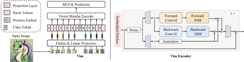
Figure 1: The overview of the Vim model.

3.4 Overview of Vim

As shown in Figure 1, Vim first reshapes the 2D image $\mathbf{X}\in\mathbb{R}^{h\times w\times c}$ into a sequence of flattened 2D patches $\mathbf{X}_{p}\in\mathbb{R}^{n\times(p^{2}\cdot c)}$, where $c$ is the number of channels, $(h,w)$ is the resolution of the original image, and $(p,p)$ is the resolution of each image patch. The effective sequence length for Vim is therefore $n=hw/p^{2}$. Then, Vim linearly projects $\mathbf{X}_{p}$ into vectors of size $d$ and adds them to the position embeddings $E_{pos}\in\mathbb{R}^{(n+1)\times d}$, as follows:

$$\mathbf{T}_{0} =[\mathbf{X}_{\mathtt{cls}};\mathbf{X}_{p}^{1}\mathbf{W};\mathbf{X}_{p}^{2}\mathbf{W};\cdots;\mathbf{X}_{p}^{i}\mathbf{W};\cdots;\mathbf{X}_{p}^{d}\mathbf{W}]+\mathbf{E}_{pos},$$ (5)

where $\mathbf{X}_{p}^{i}$ is the $i$-th patch of $\mathbf{X}$, $\mathbf{W}\in\mathbb{R}^{(p^{2}\cdot c)\times d}$ is the learnable projection matrix. Vim uses class token to represent the whole patch sequence, which is denoted as $\mathbf{X}_{\mathtt{cls}}$. Vim then sends the token sequence ($\mathbf{T}_{l-1}$) to the $l$-th layer of the Vim encoder, and gets the output $\mathbf{T}_{l}$. Finally, Vim normalizes the output class token $\mathbf{T}_{L}^{0}$ and feeds it to the multi-layer perceptron (MLP) head to get the final prediction $\hat{p}$, as follows:

$$\mathbf{T}_{l} =\mathbf{Vim}(\mathbf{T}_{l-1})+\mathbf{T}_{l-1},$$ (6)

$$\mathbf{\it f} =\mathbf{Norm}(\mathbf{T}_{L}^{0}),$$

$$\hat{p} =\mathbf{MLP}(\mathbf{\it f}),$$

where $\mathbf{Vim}$ is the proposed vision mamba block, $L$ is the number of layers, and $\mathbf{Norm}$ is the normalization layer.

4 Methodology

In this section, we commence with a thorough introduction to the scanning strategy of Vim-F. Subsequently, we present the specific details of the patch embedding in Vim-F(H). Finally, we analyze the efficiency of Vim-F(H). Through these steps, we aim to provide a comprehensive understanding of Vim-F(H).

4.1 2D scanning in the frequency domain

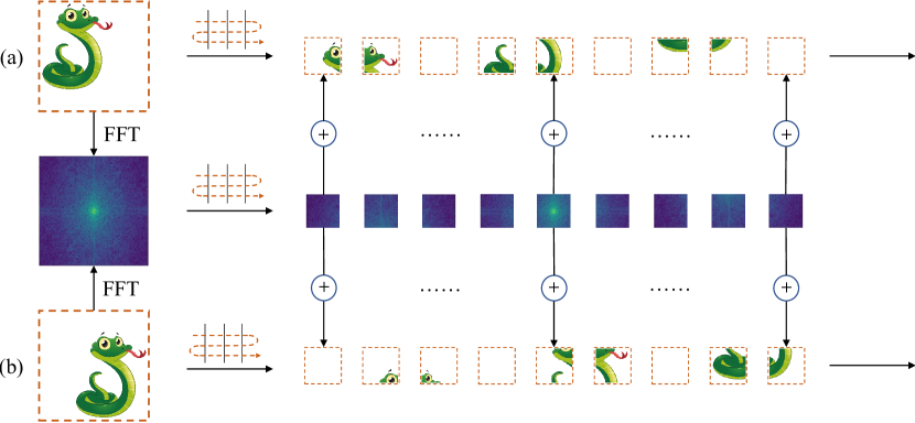
Figure 2: Illustrating the scanning strategy of Vim-F through an example of forward scanning in both the frequency and spatial domains. Due to the translation invariance of the Fourier transform, the Fourier transforms of figures (a) and (b) are identical.

As shown in Figure 1, the flattening method used in Vim disrupts these local dependencies and significantly increases the distance between vertically adjacent tokens. We address this limitation by introducing frequency-domain scanning. Specifically, we first perform a Fourier transform on the feature map to obtain:

$$F(u,v)=\sum_{x=0}^{M-1}\sum_{y=0}^{N-1}f(x,y)e^{-j2\pi\left(\frac{ux}{H}+\frac{vy}{W}\right)},$$ (7)

where $j$ represents the imaginary unit, $H$ and $W$ represent the height and width of the feature map, respectively. $f(x,y)\in\mathbb{R}^{H\times W}$ represents the corresponding value at the coordinate $(x,y)$ in the feature map, and $F(u,v)$ represents the corresponding value at the coordinate $(u,v)$ in the frequency domain. $|F(u,v)|\in\mathbb{R}^{H\times W}$ represents the modulus of $F(u,v)$, which is also known as the amplitude spectrum. Fourier transform has translation invariance. In other words, if a function is translated in the spatial domain, its Fourier transform remains the same as the original function. This property is quite meaningful for addressing the issue of increasing distances between vertically adjacent tokens, as shown in Figure 2. The amplitude spectra of figures (a) and (b) are identical, so scanning in the frequency domain helps reduce the inductive bias introduced by the scanning strategy. Therefore, frequency domain scanning does not require fancy strategies, and it can be consistent with Vim’s original spatial domain scanning strategy. Finally, we use two trainable parameters as the superposition coefficients of the feature map and the corresponding spectrogram to dynamically adjust the information intensity in the spatial and frequency domains. The Mamba encoder establishes a unified representation of visual information in the spatial and frequency domains.

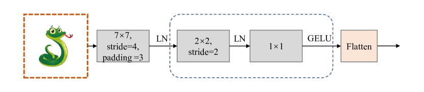
Figure 3: The overall architecture of patch embedding in Vim-F(H).

4.2 Patch embedding

The overall architecture of the patch embedding module is shown in Figure 3.

4.2.1 Convolutional stem

Table 1: Convolutional stem for patch embedding.

	Output size	Vim-Ti	Vim-S
Block1	56$\times$56	7$\times$7, 48, stride 4	7$\times$7, 48, stride 4
		padding 3	padding 3
Block2	28$\times$28	$\begin{bmatrix}\text{2$\times$2, 96, stride 2}\\ \text{1$\times$1, 96}\end{bmatrix}$	$\begin{bmatrix}\text{2$\times$2, 192, stride 2}\\ \text{1$\times$1, 192}\end{bmatrix}$
Block3	14$\times$14	$\begin{bmatrix}\text{2$\times$2, 192, stride 2}\\ \text{1$\times$1, 192}\end{bmatrix}$	$\begin{bmatrix}\text{2$\times$2, 384, stride 2}\\ \text{1$\times$1, 384}\end{bmatrix}$

In Vim and ViTs, the patching strategy typically involves using large convolutional kernels (such as kernel sizes of 14 or 16) with non-overlapping convolutions. However, VMamba and Swin Transformer utilize non-overlapping convolutions with a kernel size of 4, indicating that current ViMs haven’t undergone much targeted design in terms of patching. We believe that non-overlapping convolutions have fewer inductive biases, and the self-attention mechanism of the Transformer architecture excels at modeling relationships between patches. Therefore, adopting non-overlapping convolutions can benefit the performance of Transformers. On the contrary, the additional correlation between patches introduced by overlapping convolutions can be advantageous for the scanning mechanism of ViMs.

Based on the above analysis, we can try to explain why Vim uses the position embedding. The bidirectional horizontal scanning strategy employed by Vim makes adjacent tokens in horizontal and vertical directions far apart in the sequence. In addition, the lack of data correlation between tokens makes it difficult for the model to understand the spatial relationship in the vertical direction. The introduction of the trainable position embedding can explicitly provide the model with the absolute position of each token in the plane space, thus alleviating the above problems. In contrast, it is simpler and more flexible to remove the position embedding and establish spatial correlation through overlapping convolutions, enabling the model to learn spatial positional relationships.

Specifically, we first utilize a $7\times 7$ convolutional layer with a stride of 4 to model the local correlation of the input image. Then, we downsample the feature map twice through two downsampling blocks. Each downsampling block consists of a $2\times 2$ convolutional layer with a stride of 2 and a $1\times 1$ convolutional layer. The details of the adaptation with the two base models Zhu et al., (2024) (Vim-Ti and Vim-S) are shown in Table 1 and Figure 3.

4.3 Efficiency analysis

Vim-F requires a 2D discrete Fourier transform (DFT) to be performed on the feature map before scanning, thus introducing additional computation. The Cooley-Tukey FFT algorithm decomposes a DFT of a sequence with length N into two DFTs of sub-sequences with length N/2, significantly reducing the computational complexity. During the execution of the algorithm, the data is divided into two parts based on whether they are odd or even, and the DFTs of each part are computed separately before merging the results. For a 2D-DFT with dimensions $(H,W)$, its complexity is approximately $O(H\cdot W\cdot log(H)\cdot log(W))$. Compared to the overall computational complexity of the model, the computational cost of this part can be negligible.

The patch embedding in Vim can be implemented through a $16\times 16$ convolutional layer with a stride of 16. The convolutional stem for patch embedding in Vim-F(H) comprises more convolutional layers, but the computational cost increases moderately due to the use of smaller convolutional kernels. Considering Vim-Ti as the baseline model, the computational load measured in GFLOPs only increases by 0.035. In summary, there is no significant difference in computational cost between Vim-F(H) and Vim. LocalVimHuang et al., (2024) is one of the representative works that improve the scanning strategy for Vim. In terms of efficiency, LocalVim’s selective scanning branches are twice as many as our Vim-F(H), and it uses a complex spatial and channel attention module (SCAttn) to weight the channels and tokens in the features of each branch. Therefore, our Vim-F(H) achieves a better balance between performance and efficiency.

Table 2: Comparison of different backbones on ImageNet-1K classification. $\dagger:$ We are unable to reproduce the results through the source code provided by the author, and one possible reason is the significant difference in hardware and the use of linear scaling rule. The results in () are from the original paper.

Method	Params (M)	FLOPs (G)	Top-1 (%)
PVTv2-B0 Wang et al., (2022)	3	0.6	70.5
DeiT-Ti Touvron et al., (2021)	6	1.3	74.4
MobileViT-XS Mehta and Rastegari, (2021)	2	1.0	74.8
LVT Yang et al., (2022)	6	0.9	74.8
Vim-Ti$\dagger$ Zhu et al., (2024)	7	1.5	74.7(76.1)
Vim-Ti-F(H) (ours)	7	1.5	76.0
LocalVim-T Huang et al., (2024)	8	1.5	76.5
RegNetY-1.6G Radosavovic et al., (2020)	11	1.6	78.0
MobileViT-S Mehta and Rastegari, (2021)	6	2.0	78.4
EfficientVMamba-S Pei et al., (2024)	11	1.3	78.7
DeiT-S Touvron et al., (2021)	22	4.6	79.8
RegNetY-4G Radosavovic et al., (2020)	21	4.0	80.0
Swin-T Liu et al., (2021)	29	4.5	81.3
Vim-S$\dagger$ Zhu et al., (2024)	26	5.1	79.6(80.5)
Vim-S-F(H) (ours)	26	5.1	80.4
LocalVim-SHuang et al., (2024)	28	4.8	81.0
EfficientVMamba-BPei et al., (2024)	33	4.0	81.8
VMamba-T Liu et al., (2024)	22	5.6	82.2

5 Experiments

This section presents our experimental results, starting with the ImageNet classification task and then transferring the trained model to various downstream tasks, including object detection and instance segmentation.

5.1 Image classification

Settings. We train the models on ImageNet-1K and evaluate the performance on ImageNet-1K validation set. For fair comparisons, our training settings mainly follow Vim. Specifically, we apply random cropping, random horizontal flipping, label-smoothing regularization, mixup, and random erasing as data augmentations. When training on $224\times 224$ input images, we employ AdamW with a momentum of 0.9 and a weight decay of 0.05 to optimize models. During testing, we apply a center crop on the validation set to crop out $224\times 224$ images. We train the Vim-F(H) models for 300 epochs using a cosine schedule and EMA. Unlike Vim, our experiments are performed on 3 A6000 GPUs. Therefore, we adjusted the total batch size and the initial learning rate to 384 and $3.75\times 10^{-4}$ respectively according to the linear scaling ruleGoyal et al., (2017).

Results. We selected advanced CNNs, ViTs, and ViMs with comparable parameters and computational costs in recent years to compare with our method, and the results are shown in Table 2. Compared to our seminal Vim, our method has made substantial progress, with Vim-Ti-F(H) and Vim-S-F(H) achieving 1.3% and 0.8% higher accuracy than Vim-Ti and Vim-S, respectively. It is worth noting that SOTA ViMs such as VMamba Liu et al., (2024), LocalMamba Huang et al., (2024), and EfficientVMamba Pei et al., (2024) all adopt more complex hybrid encoding architectures, even introducing attention mechanisms. However, Vim-F still uses a pure SSM encoder to model visual information. Vim-Ti-F(H) achieves superior accuracy compared to highly optimized lightweight ViT variants, including DeiT-TiTouvron et al., (2021), MobileViT-XS Mehta and Rastegari, (2021), and LVT Yang et al., (2022), while also narrowing the gap in performance between Vim and other leading ViMs.

Long sequence fine-tuning. ViM with a pure Mamba encoder can compress signals at a low cost and reconstruct them into longer sequences. For visual tasks, flattening images into longer 1D sequences and fine-tuning the model can allow the model to capture more details and improve performance. Due to the use of absolute position embedding, Vim needs to expand the encoding length through interpolation methods. In addition, because the position embedding is located at the front of the entire network, more epochs of fine-tuning are required for adaptation. We set the stride of the first convolutional layer in the patch embedding to 2, and set the learning rate to $1\times 10^{-5}$ for 1 epoch of fine-tuning. Vim-Ti-F(H) can achieve a 0.8% increase in accuracy.

Table 3: The classification result of Vim-F(H) on ImageNet-1K after 1 epoch of fine-tuning. Different from the pre-training stage, the input image is flattened into 784 tokens (28$\times$28).

Method	Params (M)	Top-1 (%)
Vim-Ti-F(H) (Fine-tuning for 1 epoch)	7	76.8
Vim-S-F(H) (Fine-tuning for 1 epoch)	26	81.2

Table 4: Object detection and instance segmentation results on COCO.

Mask R-CNN 1$\times$ schedule
Backbone	Params	FLOPs	APb	AP${}^{\mathrm{b}}_{50}$	AP${}^{\mathrm{b}}_{75}$	APm	AP${}^{\mathrm{m}}_{50}$	AP${}^{\mathrm{m}}_{75}$
LightViT-T	28M	187G	37.8	60.7	40.4	35.9	57.8	38.0
ResNet-18	31M	207G	34.0	54.0	36.7	31.2	51.0	32.7
EfficientVMamba-S	31M	197G	39.3	61.8	42.6	36.7	58.9	39.2
PVT-T	33M	208G	36.7	59.2	39.3	35.1	56.7	37.3
ResNet-50	44M	260G	38.2	58.8	41.4	34.7	55.7	37.2
LocalVMamba-T	45M	291G	46.7	68.7	50.8	42.2	65.7	45.5
Swin-T	48M	267G	42.7	65.2	46.8	39.3	62.2	42.2
ConvNeXt-T	48M	262G	44.2	66.6	48.3	40.1	63.3	42.8
ViT-Adapter-S	48M	403G	44.7	65.8	48.3	39.9	62.5	42.8
ResNet-101	63M	336G	38.2	58.8	41.4	34.7	55.7	37.2
Swin-S	69M	354G	44.8	66.6	48.9	40.9	63.2	44.2
ConvNeXt-S	70M	348G	45.4	67.9	50.0	41.8	65.2	45.1
Vim-Ti	27M	189G	36.6	59.4	39.2	34.9	56.7	37.3
Vim-Ti-F(H) (ours)	27M	189G	37.7	60.8	40.9	35.7	57.8	37.9
Vim-S	44M	272G	42.9	65.4	47.1	39.2	62.1	42.1
Vim-S-F(H) (ours)	44M	272G	43.1	65.2	47.3	39.3	62.2	42.3

5.2 Object detection and instance segmentation

Settings. We use Mask-RCNN as the detector to evaluate the performance of the proposed Vim-F(H) for object detection and instance segmentation on the MSCOCO 2017 dataset. Since the backbone of Vim-F(H) is non-hierarchical, following ViTDetLi et al., (2021), we only used the last feature map from the backbone and generated multi-scale feature maps through a set of convolutions or deconvolutions to adapt to the detector. The remaining settings were consistent with SwinLiu et al., (2021). Specifically, we employ the AdamW optimizer and fine-tune the pre-trained classification models (on ImageNet-1K) for both 12 epochs (1$\times$ schedule). The learning rate is initialized at $1\times 10^{-4}$ and is reduced by a factor of $10\times$ at the 9th and 11th epochs.

Results. We summarize the comparison results of Vim-F(H) with other backbones in Table 4. It can be seen that our Vim-F(H) consistently outperforms Vim. Similar to the results on classification tasks, Vim-F(H) with a pure SSM encoder achieves a good balance between the number of parameters and computational cost, achieving comparable results with advanced CNNs and ViTs.

6 Conclusion and limitation

One of the main challenges currently faced by ViMs is the destruction of local two-dimensional dependency relationships when spatial data is flattened into one-dimensional tokens due to the non-causal nature of visual data. Consequently, scanning one-dimensional tokens with specific rules can limit the model’s ability to accurately interpret spatial relationships. We observed that scanning in the frequency domain, leveraging the translation invariance and global nature of Fourier transforms, can reduce the inductive bias of scanning strategies while ensuring that the model always maintains a good global receptive field. We adopted a simple approach of adding the spectrogram with the original feature map, allowing the model to scan simultaneously in both the frequency and spatial domains, thereby establishing a unified representation of visual information across both domains. Furthermore, we employ two trainable parameters to dynamically adjust the information intensity in the frequency and spatial domains, aiming to reduce semantic gaps. We also introduce additional local correlations during patch embedding by using overlapping convolutions. Our Vim-F(H) is motivated by a simple idea and is easy to implement. Extensive experiments have demonstrated that it effectively improves the performance of Vim, achieving competitive results compared to advanced ViTs, CNNs, and ViMs. The effectiveness of our method for ViMs with hybrid encoders has not been fully studied.

Appendix A Appendix

A.1 Ablation study

Effect of frequency domain scanning. We evaluated the scanning strategy of Vim-F, and the experimental details are shown in Table 5. As mentioned earlier, position embeddings are crucial for Vim, and removing them leads to a 1.7% performance drop for Vim-Ti. However, the global receptive field brought by frequency domain scanning reduces the model’s dependence on positional embeddings, resulting in a smaller performance drop for Vim-Ti-F. When both models use positional embeddings, Vim-Ti-F outperforms Vim-Ti by 0.4%.

Effect of convolutional stem. As shown in Table 5, further replacing the traditional patch embedding in Vim-Ti with our proposed convolutional stem leads to a 0.9% improvement in performance. This shows that introducing additional local correlation into the patch embedding is effective.

Table 5: Ablation study of frequency domain scanning and patch embedding in Vim-Ti-F(H) on ImageNet-1K.

Model	Top-1 (%)
Vim-Ti (without Position Embedding)	73.0%
Vim-Ti (base)	74.7%
Vim-Ti-F	74.2%
Vim-Ti-F + Position Embedding	75.1%
Vim-Ti-F(H)	76.0%

References

- Dai et al., (2021) Dai, Z., Liu, H., Le, Q. V., and Tan, M. (2021). Coatnet: Marrying convolution and attention for all data sizes. In Advances in Neural Information Processing Systems (NeurIPS), pages 3965–3977.
- Dosovitskiy et al., (2021) Dosovitskiy, A., Beyer, L., Kolesnikov, A., Weissenborn, D., Zhai, X., Unterthiner, T., Dehghani, M., Minderer, M., Heigold, G., Gelly, S., Uszkoreit, J., and Houlsby, N. (2021). An image is worth 16x16 words: Transformers for image recognition at scale. In 9th International Conference on Learning Representations (ICLR).
- Goyal et al., (2017) Goyal, P., Dollár, P., Girshick, R. B., Noordhuis, P., Wesolowski, L., Kyrola, A., Tulloch, A., Jia, Y., and He, K. (2017). Accurate, large minibatch SGD: training imagenet in 1 hour. Preprint arXiv:2111.11429.
- Gu and Dao, (2023) Gu, A. and Dao, T. (2023). Mamba: Linear-time sequence modeling with selective state spaces. Preprint arxiv:2312.00752.
- Gupta et al., (2022) Gupta, A., Gu, A., and Berant, J. (2022). Diagonal state spaces are as effective as structured state spaces. In Advances in Neural Information Processing Systems (NeurIPS).
- He et al., (2016) He, K., Zhang, X., Ren, S., and Sun, J. (2016). Deep residual learning for image recognition. In Proceedings of the IEEE conference on computer vision and pattern recognition (CVPR), pages 770–778.
- Howard et al., (2017) Howard, A. G., Zhu, M., Chen, B., Kalenichenko, D., Wang, W., Weyand, T., Andreetto, M., and Adam, H. (2017). Mobilenets: Efficient convolutional neural networks for mobile vision applications. Preprint arXiv:1704.04861.
- Huang et al., (2017) Huang, G., Liu, Z., Van Der Maaten, L., and Weinberger, K. Q. (2017). Densely connected convolutional networks. In Proceedings of the IEEE conference on computer vision and pattern recognition (CVPR), pages 4700–4708.
- Huang et al., (2024) Huang, T., Pei, X., You, S., Wang, F., Qian, C., and Xu, C. (2024). Localmamba: Visual state space model with windowed selective scan. Preprint arXiv:2403.09338.
- Lee-Thorp et al., (2022) Lee-Thorp, J., Ainslie, J., Eckstein, I., and Ontañón, S. (2022). Fnet: Mixing tokens with fourier transforms. In Proceedings of the 2022 Conference of the North American Chapter of the Association for Computational Linguistics: Human Language Technologies (NAACL), pages 4296–4313.
- Li et al., (2021) Li, Y., Xie, S., Chen, X., Dollár, P., He, K., and Girshick, R. B. (2021). Benchmarking detection transfer learning with vision transformers. Preprint arXiv:2111.11429.
- Li et al., (2022) Li, Y., Yuan, G., Wen, Y., Hu, J., Evangelidis, G., Tulyakov, S., Wang, Y., and Ren, J. (2022). Efficientformer: Vision transformers at mobilenet speed. In Annual Conference on Neural Information Processing Systems (NeurIPS).
- Liu et al., (2024) Liu, Y., Tian, Y., Zhao, Y., Yu, H., Xie, L., Wang, Y., Ye, Q., and Liu, Y. (2024). Vmamba: Visual state space model. Preprint arXiv:2401.10166.
- Liu et al., (2021) Liu, Z., Lin, Y., Cao, Y., Hu, H., Wei, Y., Zhang, Z., Lin, S., and Guo, B. (2021). Swin transformer: Hierarchical vision transformer using shifted windows. In 2021 IEEE/CVF International Conference on Computer Vision (ICCV), pages 9992–10002.
- Mehta et al., (2023) Mehta, H., Gupta, A., Cutkosky, A., and Neyshabur, B. (2023). Long range language modeling via gated state spaces. In The Eleventh International Conference on Learning Representations (ICLR).
- Mehta and Rastegari, (2021) Mehta, S. and Rastegari, M. (2021). Mobilevit: light-weight, general-purpose, and mobile-friendly vision transformer. Preprint arXiv:2110.02178.
- Mehta and Rastegari, (2022) Mehta, S. and Rastegari, M. (2022). Mobilevit: Light-weight, general-purpose, and mobile-friendly vision transformer. In The Tenth International Conference on Learning Representations (ICLR).
- Pei et al., (2024) Pei, X., Huang, T., and Xu, C. (2024). Efficientvmamba: Atrous selective scan for light weight visual mamba. Preprint arxiv:2403.09977.
- Pratt et al., (2017) Pratt, H., Williams, B., Coenen, F., and Zheng, Y. (2017). Fcnn: Fourier convolutional neural networks. In Machine Learning and Knowledge Discovery in Databases: European Conference (ECML), pages 786–798.
- Radosavovic et al., (2020) Radosavovic, I., Kosaraju, R. P., Girshick, R., He, K., and Dollár, P. (2020). Designing network design spaces. In Proceedings of the IEEE conference on computer vision and pattern recognition (CVPR), pages 10428–10436.
- Rao et al., (2021) Rao, Y., Zhao, W., Zhu, Z., Lu, J., and Zhou, J. (2021). Global filter networks for image classification. In Advances in Neural Information Processing Systems (NeurIPS), pages 980–993.
- Ruan and Xiang, (2024) Ruan, J. and Xiang, S. (2024). Vm-unet: Vision mamba unet for medical image segmentation.
- Simonyan and Zisserman, (2014) Simonyan, K. and Zisserman, A. (2014). Very deep convolutional networks for large-scale image recognition. Preprint arXiv:1409.1556.
- Srinivas et al., (2021) Srinivas, A., Lin, T.-Y., Parmar, N., Shlens, J., Abbeel, P., and Vaswani, A. (2021). Bottleneck transformers for visual recognition. In Proceedings of the IEEE Conference on Computer Vision and Pattern Recognition (CVPR), pages 16519–16529.
- Szegedy et al., (2015) Szegedy, C., Liu, W., Jia, Y., Sermanet, P., Reed, S., Anguelov, D., Erhan, D., Vanhoucke, V., and Rabinovich, A. (2015). Going deeper with convolutions. In Proceedings of the IEEE conference on computer vision and pattern recognition (CVPR), pages 1–9.
- Tamkin et al., (2020) Tamkin, A., Jurafsky, D., and Goodman, N. (2020). Language through a prism: A spectral approach for multiscale language representations. In Advances in Neural Information Processing Systems((NeurIPS), pages 5492–5504.
- Tan and Le, (2019) Tan, M. and Le, Q. (2019). Efficientnet: Rethinking model scaling for convolutional neural networks. In International conference on machine learning (ICML), pages 6105–6114.
- Touvron et al., (2021) Touvron, H., Cord, M., Douze, M., Massa, F., Sablayrolles, A., and Jégou, H. (2021). Training data-efficient image transformers & distillation through attention. In International conference on machine learning (ICML), pages 10347–10357.
- Wang et al., (2022) Wang, W., Xie, E., Li, X., Fan, D.-P., Song, K., Liang, D., Lu, T., Luo, P., and Shao, L. (2022). Pvt v2: Improved baselines with pyramid vision transformer. Computational Visual Media, 8(3):415–424.
- Wang et al., (2024) Wang, Z., Zheng, J.-Q., Zhang, Y., Cui, G., and Li, L. (2024). Mamba-unet: Unet-like pure visual mamba for medical image segmentation.
- Xie et al., (2017) Xie, S., Girshick, R., Dollár, P., Tu, Z., and He, K. (2017). Aggregated residual transformations for deep neural networks. In Proceedings of the IEEE conference on computer vision and pattern recognition (CVPR), pages 1492–1500.
- Yang et al., (2022) Yang, C., Wang, Y., Zhang, J., Zhang, H., Wei, Z., Lin, Z., and Yuille, A. (2022). Lite vision transformer with enhanced self-attention. In Proceedings of the IEEE Conference on Computer Vision and Pattern Recognition (CVPR), pages 11998–12008.
- Zhang et al., (2018) Zhang, J., Lin, Y., Song, Z., and Dhillon, I. (2018). Learning long term dependencies via Fourier recurrent units. In Proceedings of the 35th International Conference on Machine Learning (ICML), pages 5815–5823.
- Zhu et al., (2024) Zhu, L., Liao, B., Zhang, Q., Wang, X., Liu, W., and Wang, X. (2024). Vision mamba: Efficient visual representation learning with bidirectional state space model. Preprint arXiv:2401.09417.