Deep Bayesian Filter for Bayes-faithful Data Assimilation

Abstract

State estimation for nonlinear state space models is a challenging task. Existing assimilation methodologies predominantly assume Gaussian posteriors on physical space, where true posteriors become inevitably non-Gaussian. We propose Deep Bayesian Filtering (DBF) for data assimilation on nonlinear state space models (SSMs). DBF constructs new latent variables $h_{t}$ on a new latent (“fancy”) space and assimilates observations $o_{t}$. By (i) constraining the state transition on fancy space to be linear and (ii) learning a Gaussian inverse observation operator $q(h_{t}|o_{t})$, posteriors always remain Gaussian for DBF. Quite distinctively, the structured design of posteriors provides an analytic formula for the recursive computation of posteriors without accumulating Monte-Carlo sampling errors over time steps. DBF seeks the Gaussian inverse observation operators $q(h_{t}|o_{t})$ and other latent SSM parameters (e.g., dynamics matrix) by maximizing the evidence lower bound. Experiments show that DBF outperforms model-based approaches and latent assimilation methods in various tasks and conditions.

1 Introduction

Data assimilation (DA) is a central technique for various scientific domains. The primary objective of DA is to utilize an imperfect system model and partially informative observations to give the statistically best estimate of the trajectory and the current state. DA has been applied to various fields, such as weather forecasting (Hunt et al., 2007; Lorenc, 2003; Andrychowicz et al., 2023), sea surface temperature prediction (Larsen et al., 2007), analysis of seismic waves (Alfonzo and Oliver, 2020), multi-sensor fusion localization (Bach and Ghil, 2023), and object tracking (Awal et al., 2023).

Albeit its importance, DA remains a challenging task except for the Linear Gaussian State Space (LGSS) model, where the Kalman Filter (KF) algorithm (Kalman, 1960) allows analytical computation of posteriors. If either the observation operator or the dynamics operator is nonlinear, posteriors become non-Gaussian, making the analytic computation intractable. Existing nonlinear filtering methods such as the ensemble Kalman Filter (Evensen, 1994; Bishop et al., 2001) often assume Gaussian for posteriors on physical space, inevitably introducing biases. Although Particle Filters and other sequential Monte Carlo methods have been steadily developed (Daum and Huang, 2007; Hu and van Leeuwen, 2021), more satisfactory algorithms still need to be established for high-dimensional problems.

This paper proposes a novel methodology for posterior estimate, named Deep Bayesian Filtering (DBF). It assumes a state space model (SSM) whose state transition model is linear Gaussian, but the observation operator is nonlinear. Specifically, we approximate the inverse observation operator (IOO) (Frerix et al., 2021), which is a mapping from the observation space to the state space, using a Gaussian distribution with the assistance of neural networks (NNs). For nonlinear dynamics problems, following the variational auto-encoder (VAE) structure, DBF approximates a posterior with a Gaussian distribution on a latent space by creating variables that follow linear dynamics on the space. With this formulation, we describe the update equation for sequential Bayesian inference, which yields the filter distribution with a structure similar to the exact posterior update equations. DBF naturally generalizes the KF.

DBF is a VAE faithful to the Markov property for SSM with nonlinear dynamics. Posterior distributions of latent variables are expressed in a Bayes-faithful form. A closely relevant class of models is dynamical VAE (DVAE, Girin et al. 2021 for a review), which utilizes the VAE structure for modeling time-series data. The idea of modeling dynamics on a latent space and training the model through maximizing evidence lower-bound (ELBO) is the same as DBF. A notable feature that differentiates our proposed method is the design of posteriors. In DBF, the Bayes-faithful structure of posteriors allows analytical integration of the prediction step (computation of $\tilde{p}(h_{t}|o_{1:t-1})$ from $\tilde{p}(h_{t-1}|o_{1:t-1})$, where $h_{t},o_{t}$ are latent and observed variables at step $t$, and $\tilde{p}$ is the probability distribution function of $h_{t}$ constructed by the model). All the posteriors can be recursively computed by analytic formulae, in contrast to DVAE methods, where Monte Carlo sampling is inevitable for the integration of $h_{1:t}$.

In the case of applying DBF to problems with nonlinear or unknown dynamics, we can interpret that DBF learns the Koopman operator (Koopman, 1931) using NNs. Data-driven discovery of such latent space and the operator using machine learning is extensively investigated (Takeishi et al., 2017; Lusch et al., 2018; Azencot et al., 2020). Its applicability is experimentally demonstrated by handling nonlinear filtering tasks with chaotic dynamics.

We summarize the prominent properties of the proposed methodology.

• DBF is the first VAE model that assumes a posterior structure faithful to the Markov property of a SSM.

• For SSM with linear dynamics, DBF extends the celebrated KF to accept nonlinear observations using learnable neural networks. It facilitates learning of unknown system parameters from data (see Section 3.1).

• For nonlinear dynamics problems, DBF constructs a new latent space for DA. DBF avoids accumulating Monte-Carlo sampling errors in forward time steps by computing the integration over time analytically. Thanks to the theory of the Koopman operator, the linear constraint on dynamics does not limit the representation power, provided that the dimension of the latent space is sufficiently high (see Sections 3.2 and 3.3).

• As a generative model, DBF gives the uncertainty of the estimate $z_{t}$, in contrast to other methodologies for regression that end up as a point estimate (see Section 3.2 and Figure 2).

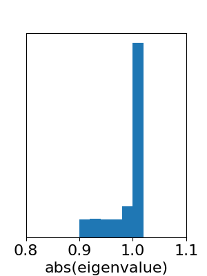
setting	max(|eig|)
D, $\sigma=1$	$1.016\pm 0.002$
D, $\sigma=3$	$1.014\pm 0.002$
D, $\sigma=5$	$1.011\pm 0.001$
N, $\sigma=1$	$1.012\pm 0.003$
N, $\sigma=3$	$1.008\pm 0.004$
N, $\sigma=5$	$1.004\pm 0.001$

Figure 4: Histogram of 800 eigenvalues of the dynamics matrix in Lorenz96. D for direct and N for nonlinear observations.

• The linear constraint on dynamics stabilizes the training, which was unstable with standard recurrent neural networks (see Section 3.3 and Figure 4).

In problem settings with highly non-Gaussian posteriors, such as strongly nonlinear observation operators or large noises, DBF outperforms classical DA algorithms and latent assimilation methods.

2 State space model

Let $h_{t}$ and $o_{t}$ denote the latent state (just referred to as state) and observation at time $t$, and $h_{t:T}$ and $o_{t:T}$ denote the time series of the state and observation from time $t$ to $T$, respectively. The discrete-time SSM consists of a state transition model $p(h_{t+1}|h_{t})$ and an observation model $p(o_{t}|h_{t})$. Due to the Markov property, we can factorize the joint distribution of the state and observation time series as $p(o_{1:t},h_{1:t})=\prod_{k=1}^{t}p(o_{t}|h_{t})p(h_{t}|h_{t-1})$. Here, we have used the convention $p(h_{1}|h_{0})=p(h_{1})$ to represent the initial distribution $p(h_{1})$.

The posterior distribution of a state $h_{T}$ given the observation time series $o_{1:t}$ ($t<T$) is computed from a filter distribution $p(h_{t}|o_{1:t})$ and the transition model:

$$p(h_{T}|o_{1:t})=\int\left(\prod_{k=t}^{T}p(h_{k}|h_{k-1})\right)p(h_{t}|o_{1:t})dh_{t:T-1}.$$ (1)

We can factorize the filter distribution recursively following the Bayes’ rule and the Markov property: $p(h_{t}|o_{1:t})=p(o_{t}|h_{t})p(h_{t}|o_{1:t-1})/p(o_{t}|o_{1:t-1})$, where

$$p(o_{t}|o_{1:t-1})=\int p(o_{t}|h_{t})\int p(h_{t}|h_{t-1})p(h_{t-1}|o_{1:t-1})dh_{t-1:t}.$$ (2)

Thus, the primary objective of DA is to compute the filter distribution.

2.1 Kalman Filter (KF)

In KF, the dynamics and the observation models are both linear Gaussians, with the mean being linear with respect to the conditional variable and a constant covariance matrix.

$$p(h_{t+1}|h_{t}) = \mathcal{N}(h_{t+1}|Ah_{t},Q),$$ (3)

$$p(o_{t}|h_{t}) = \mathcal{N}(o_{t}|Ch_{t},R),$$ (4)

where $\mathcal{N}(x|\mu,\Sigma)$ denotes a Gaussian whose mean and covariance are $\mu$ and $\Sigma$. The matrices $A,C,Q$, and $R$ are constant. Because both models are linear Gaussians, the filter distribution $p(h_{t}|o_{1:t})$ is also a Gaussian, provided that the initial distribution is a Gaussian. We can compute parameters for the posteriors (means $\mu_{t|t}$ and covariance matrices $\Sigma_{t|t}$) recursively from the previous step via analytical formula.

2.2 Deep Bayesian Filter (DBF)

2.2.1 Recursive formula

To start, we rewrite the recursive formula for the filter distribution as follows.

$$p(h_{t}|o_{1:t}) = \frac{p(o_{t}|h_{t})p(h_{t}|o_{1:t-1})}{p(o_{t}|o_{1:t-1})}\propto\frac{q(h_{t}|o_{t})}{\rho(h_{t})}p(h_{t}|o_{1:t-1}),$$ (5)

where $q(h_{t}|o_{t})=\frac{p(o_{t}|h_{t})\rho(h_{t})}{\int p(o_{t}|h_{t})\rho(h_{t})dh_{t}}$. We have introduced $\rho(h_{t})$, a virtual “prior” of the latent variable $h_{t}$. The proportionality holds for the variable $h_{t}$ as $p(o_{t}|o_{1:t-1})$ does not depend on $h_{t}$.

We call $q(h_{t}|o_{t})$ an inverse observation operator (IOO) because it puts density on the latent space opposite to the observation model that puts density on the observation space. We approximate the IOO, $q(h_{t}|o_{t})$, and $\rho(h_{t})$ with Gaussians;

$$q(h_{t}|o_{t}) = \mathcal{N}(h_{t}|f_{\theta}(o_{t}),G_{\theta}(o_{t})),$$ (6)

$$\rho(h_{t}) = \mathcal{N}(h_{t}|m,V),$$ (7)

where $f_{\theta}(o_{t})$ and $G_{\theta}(o_{t})$ are NNs parameterized by $\theta$. Parameters for the virtual prior ($m$ and $V$) are fixed at $m=0$ and $V=10^{8}I$ during experiments. These parameters do not affect training results as long as $V^{-1}$ is sufficiently small. Hereafter, we will denote the approximate posterior as $\tilde{p}(h_{t}|o_{1:t})$. The IOO and its parameters are included in $\tilde{p}(h_{t}|o_{1:t})$.

With Gaussian assumptions for the IOO $q(h_{t}|o_{t})$ and the virtual prior $\rho(h_{t})$, all approximate posteriors $\tilde{p}(h_{t}|o_{1:t})$ are Gaussians (see Eq. (5)). Therefore, we can analytically compute $\tilde{p}(h_{t}|o_{1:t})=\mathcal{N}(h_{t}|\mu_{t},\Sigma_{t})$ while ignoring the normalization factor $p(o_{t}|o_{1:t-1})$. The posterior update formula is as follows;

$$\mu_{t} = \Sigma_{t}(A\Sigma_{t-1}A^{T}+Q)^{-1}A\mu_{t-1}+G_{\theta}(o_{t})^{-1}f_{\theta}(o_{t})-V^{-1}m,$$ (8)

$$\Sigma_{t}^{-1} = (A\Sigma_{t-1}A^{T}+Q)^{-1}+G_{\theta}(o_{t})^{-1}-V^{-1}.\quad\quad$$ (9)

Here, the Gaussian parameters for $h_{t}$ distribution ($\mu_{t}$ and $\Sigma_{t}$) are modified from those of the previous step ($\mu_{t-1}$ and $\Sigma_{t-1}$) by the new observation $o_{t}$ through IOO at each timestep. The recursive structure is identical to that of RNNs. The impact of the new observation $o_{t}$ is modulated by the covariance $G_{\theta}(o_{t})$.

2.2.2 Properties of DBF

The recursive formula for the exact posterior (Eq. (5)) does not involve approximation. Therefore, DBF can compute the exact posterior when the true IOO $q_{\rm true}(h_{t}|o_{t})$ is Gaussian, i.e., the SSM is a LGSS. In that case, the posterior update formula agrees with the KF. The difference is that the nonlinear functions are allowed for the mean $f_{\theta}(o_{t})$ and the covariance matrix $G_{\theta}(o_{t})$. In KF, $f_{\theta}(o_{t})$ is a linear function, and $G_{\theta}(o_{t})$ is a constant covariance matrix of error in the observation operator. The dependence of $G_{\theta}(o_{t})$ on observations provides flexibility in adjusting the impact of the new observation on the state estimation. The importance of adjusting the internal state updates based on observations has also been discussed in recent SSM-based approaches (Gu and Dao, 2023).

It is not always possible to represent the exact posterior distribution regardless of the representation power of a neural network (NN). DBF trains NNs to provide the best posterior for $h_{t}$ given observations up to present $o_{1:t}$ under the constraint that the structure of posterior $\tilde{p}(h_{t}|o_{1:t})$ needs to be consistent with that of the sequential Bayesian filter as described in Eq. (5). This feature allows us to describe DBF as “Bayes-faithful”. When constructing posteriors $\tilde{p}(h_{t}|o_{1:t})$), DBF uses NNs only for IOO to represent its statistics conditioned on instantaneous observation.

2.2.3 Applicability to nonlinear dynamics

DBF executes DA for SSMs with nonlinear dynamics by introducing a set of latent variables $h_{t}$ on a "fancy space" alongside the original "physical space" for $z_{t}$. The state transition model in the fancy space is linear Gaussian, facilitating the assimilation procedure for physical variables by learning the embedding from observations to the fancy space.

DBF can construct fancy spaces even without access to physical variables during training. In this scenario, DBF reconstructs $o_{t}$ from $h_{t}$ with the aim of future observation predictions, though direct estimation of the hidden physical state $z_{t}$ is abandoned. The Koopman operator theory (Koopman, 1931) asserts that nonlinear dynamics can be represented as linear dynamics in an infinite-dimensional space. Data-driven discovery of such embedding with finite dimensions has been intensively investigated (Takeishi et al., 2017; Lusch et al., 2018; Azencot et al., 2020). This approach offers computational advantages, particularly in high-dimensional physical spaces like weather forecasting, where the intrinsic degrees of freedom that govern the time evolution are lower than the number of cells in a simulation. It facilitates the reduction of computational costs regardless of the high dimensionality of the physical space.

2.2.4 Training

When we assimilate on physical space (i.e., the dynamics is linear), we train only the IOO (i.e., $f_{\theta}$ and $G_{\theta}$) by optimizing the evidence lower bound (ELBO):

$$\log p(o_{1:T}) = \sum_{t=1}^{T}\log p(o_{t}|o_{1:t-1})\geq-\mathcal{L}_{\rm ELBO},$$

$$\mathcal{L}_{\rm ELBO} = -\sum_{t=1}^{T}\int\tilde{p}(h_{t}|o_{1:t})\log p(o_{t}|h_{t})dh_{t}+KL[\tilde{p}(h_{t}|o_{1:t})||\tilde{p}(h_{t}|o_{1:t-1})],$$ (10)

where $KL[p||q]$ denotes the Kullback-Leibler divergence between the distributions $p$ and $q$. For SSM with nonlinear or unknown dynamics, in addition to the IOO, we train the dynamics matrix $A$ (see Section A in the appendix for parametrization) and the emission model $p(z_{t}|h_{t})=\mathcal{N}(z_{t};\phi(h_{t}),{\rm diag}[\sigma^{2}])$, which include the “observation operator” $\phi$ that projects from $h_{t}$ to $z_{t}$ and the standard deviation $\sigma$. We optimize these parameters by maximizing a joint ELBO $\mathcal{L}_{\rm ELBO,{\rm joint}}$:

$$\log p(o_{1:T},z_{1:T}) = \sum_{t=1}^{T}\log p(o_{t},z_{t}|o_{1:t-1},z_{1:t-1})\geq-\mathcal{L}_{\rm ELBO,{\rm joint}},\hskip 99.58464pt$$

$$\mathcal{L}_{\rm ELBO,{\rm joint}} = -\sum_{t}\int\tilde{p}(h_{t}|o_{1:t})\log p(z_{t}|h_{t})dh_{t}+KL[\tilde{p}(h_{t}|o_{1:t})||\tilde{p}(h_{t}|o_{1:t-1})].$$ (11)

Here, we have neglected $\log p(o_{t}|z_{t})$ from $\log p(o_{t},z_{t}|h_{t})=\log p(o_{t}|h_{t},z_{t})+\log p(z_{t}|h_{t})=\log p(o_{t}|z_{t})+\log p(z_{t}|h_{t})$. Since $\log p(o_{t}|z_{t})$ does not depend on $h_{t}$ and its distributions, it is sufficient to include $\log p(z_{t}|h_{t})$. We have replaced $\tilde{p}(h_{t}|o_{1:t},z_{1:t})$ with its special case $\tilde{p}(h_{t}|o_{1:t})$.

2.3 Related works

We discuss related works in the order of relevance.

2.3.1 Dynamical variational autoencoders

VAEs introduce hidden states $h$, assuming observations $o$ are generated from these states. DVAE integrates RNNs into VAE to generate time-series data. The encoder maps observed time series to latent ones, while the decoder operates in reverse. These mappings, facilitated by NNs, are trained through ELBO optimization. In DVAEs, introducing state transitions in hidden states contests the conditional independence of $h_{i}$ and $h_{j}$ given observations $o_{1:T}$ with the encoder $\tilde{p}(h_{1:T}|o_{1:T})$, requiring estimation and computation using $\tilde{p}(h_{1:T}|o_{1:T})$. Concretely, the marginal likelihood and its lower bound can be expressed as:

$$\log p(o_{1:T}) \geq E_{\tilde{p}(h_{1:T}|o_{1:T})}[\log p(h_{1:T},o_{1:T})-\log\tilde{p}(h_{1:T}|o_{1:T})],$$ (12)

$$(R.H.S) = \sum_{t=1}^{T}(E_{\tilde{p}(h_{t}|o_{1:T})}[\log p(o_{t}|h_{t})]$$ (13)

$$-E_{\tilde{p}(h_{t-1}|o_{1:T})}KL[\tilde{p}(h_{t}|h_{t-1},o_{t:T})|\tilde{p}(h_{t}|h_{t-1})]).$$

For SSMs with Markov properties, the conditional distribution $\tilde{p}(h_{1:T}|o_{1:T})$ can be expressed as $\tilde{p}(h_{1:T}|o_{1:T})=\prod_{t}\tilde{p}(h_{t}|h_{t-1},o_{t:T})$. Deep Markov Models utilize this structure, while subsequent DVAEs may not assume Markov properties. Regardless of the Markov assumptions, they represent $\tilde{p}(h_{1:T}|o_{1:T})$ as conditional distributions modeled by RNNs, necessitating Monte Carlo samplings.

In DBF, we take the lower bound of each $\log p(o_{t}|o_{1:t-1})$ in $\log p(o_{1:T})=\sum_{t}\log p(o_{t}|o_{1:t-1})$:

$$\log p(o_{1:T}) \geq \sum_{t=1}^{T}(E_{\tilde{p}(h_{t}|o_{1:t})}[\log p(o_{t}|h_{t})]-KL[\tilde{p}(h_{t}|o_{1:t})|\tilde{p}(h_{t}|o_{1:t-1})]).$$ (14)

Assuming Gaussian distributions for posteriors and linear Gaussian dynamics, DBF enables the analytical integration of $\tilde{p}(h_{t}|o_{1:t-1})$, leading to a structured encoder. This structured posterior facilitates the recursive computation of the filtered distribution $\tilde{p}(h_{t}|o_{1:t})$ without Monte Carlo sampling, distinguishing it from other DVAEs. By constraining dynamics to be linear, DBF ensures exact integration without accumulating Monte Carlo sampling errors over time steps. Additionally, the linear assumption helps DBF resolve instability problems associated with training standard RNNs.

SSMs are gaining attraction for modeling long-range dependencies. S4 (Gu et al., 2022) employs linear dynamics on the latent space and learns dynamics. They propose an efficient computation algorithm, outperforming transformers in datasets with long-range dependencies. LS4 (Zhou et al., 2023) extends S4 by introducing stochasticity via a VAE-like structure. LS4 and DBF share similarities: linear SSM and Gaussian posterior approximation. However, DBF updates the mean and the covariance using a recursive formula, adhering to Bayes’ rule, while LS4 substitutes recurrence computation with convolutions, neglecting a recursive approach.

2.3.2 Kalman Filter-based methods

Various approaches have been explored to overcome the constraints of the LGSS. These include approximating the model to be linear through first-order approximations using Taylor expansions such as extended Kalman Filter, approximating the sample population with a Gaussian distribution such as ensemble Kalman Filter (EnKF; Evensen 1994), and approximating the Kalman gain using neural networks (Revach et al., 2022). The EnKF and its variants (e.g., ensemble transform Kalman Filter (ETKF; Bishop et al. 2001)) are widely used in real-time DA in operational weather forecasting systems. Because these methods follow the posterior update equations of the Kalman Filter, they may introduce limitations in terms of representation capability. Additionally, calculations involving covariance matrices and their inverses in high-dimensional observation and state spaces require special techniques and considerations. As the dimensionality increases, handling these calculations becomes more challenging and may require additional approaches to ensure computational feasibility.

2.3.3 Sampling-based methods

A Particle Filter is a classical and popular method because it can assimilate any posterior given a sufficiently large number of particles. However, placing particles with sufficient density for high-dimensional state spaces poses computational challenges. Consequently, tasks with high-dimensional state spaces suffer from a particle degeneracy problem, where the number of particles that can explain the observed data becomes very small. In contrast, DBF directly learns where to place the density in the state space through IOO, which is advantageous for tasks with high-dimensional state spaces. Particle Flow Filter (PFF, Daum and Huang 2007) is an emerging method that overcomes particle degeneracy by moving particles according to the gradient flow. Recent studies show good scalability of PFF to nonlinear SSMs with hidden state dimensions as large as 1000 (Hu and van Leeuwen, 2021).

2.3.4 approximate MAP estimation method

MAP estimation is employed to find the high-density point of the posterior in high-dimensional space, such as in weather forecasting Lorenc (2003); Frerix et al. (2021). Even if the computation of the posterior $p(h_{t}|o_{1:t})$ is intractable, we may be able to perform the optimization $\log p(h_{t}|o_{1:t})=\log p(o_{t}|h_{t})+\log p(h_{t}|o_{1:t-1})$ if we can describe the function $p(o_{t}|h_{t})$ and $p(h_{t}|o_{1:t-1})=\int p(h_{t}|h_{t-1})p(h_{t-1}|o_{1:t-1})dh_{t-1}$ explicitly. In practice, we cannot access $p(h_{t-1}|o_{1:t-1})$ and cannot explicitly compute the integral $\int p(h_{t}|h_{t-1})p(h_{t-1}|o_{1:t-1})dh_{t-1}$. In that case, we only compute the mean. The downside is that the sequential computation of the covariance matrix of $p(h_{t}|o_{1:t-1})$ is impossible.

2.3.5 NN-based PDE surrogate

Recently, there have been attempts to approximate partial differential equations (PDEs) using neural networks. We also tried one of the latest methods, PDE-refiner  (Lippe et al., 2023), in the experiments of this study. However, its performance was poor, and we decided not to include it in the experiments. We suspect this is because PDE-refiner was designed to construct PDE surrogates and did not consider the noisy observation process. As a result, it was susceptible to noise. We confirmed that it can make reasonable predictions when no noise is added to observations.

3 Experiments

We evaluate the assimilation performance of DBF against three tasks. DBF utilizes the original space for the linear dynamics problem (moving MNIST). Only the IOO parameters ($f_{\theta},G_{\theta}$) are trained in this case. We compare its performance against classical DA algorithms (EnKF, ETKF, PF). For nonlinear dynamics problems (double pendulum and Lorenz96), DBF constructs a fancy space in addition to the original physical space. In addition to the IOO parameters ($f_{\theta},G_{\theta}$), we train the dynamics matrix $A$, observation operator $\phi$, and the standard deviation of the emission model $p(z_{t}|h_{t})$. We compare DBF with the classical DA algorithms and state-of-the-art assimilation methodologies (PFF, KalmanNet, DVAE-based approaches: DKF, VRNN, SRNN). We train DBF using the loss function in Eq. (11). Details on the training settings are presented in the appendix.

3.1 Moving MNIST

DBF utilizes the original physical space for DA if the dynamics operator is linear. As an example of such a problem, we consider a setting in which an image is embedded in a figure of larger size, and its position is moving at a constant velocity. When the image reaches the edge, it bounces back (the velocity is inverted) and travels in the opposite direction.

We take positions $(x,y)$ and velocities $(v_{x},v_{y})$ as physical variables, constituting a total physical space of four dimensions. The dynamics matrix is block-diagonal of two-dimension translation matrix $A_{tr}$: $A_{tr}=\begin{pmatrix}1&1\\ 0&1\\ \end{pmatrix},z_{t}=\begin{pmatrix}x_{t}\\ v_{x_{t}}\\ \end{pmatrix}$. The first block acts on $(x,v_{x})$ and the second on $(y,v_{y})$ coordinates. Observations are corrupted by additive Gaussian noise of $\sigma=10$ on each pixel. The original image is expressed as pixel values of $0$–$255$ (see appendix for an example figure).

We consider two experimental settings: image-informed and image-agnostic. In the image-agnostic setting, we do not inform the model of the embedded image: DBF prepares a learnable image tensor. EnKF, ETKF, and PF expand the system dimension by the figure size ($28\times 28=784$) and assimilate them with the original four variables.

Figure 1 shows RMSE for the estimated positions. We could not compare with KalmanNet as it requires $x_{\rm dim}^{2}$ dimensions for the input to the GRU, where $x_{\rm dim}=1936$ is too high to fit into the memory of our GPU. In image-informed settings, DBF, EnKF, and ETKF determine the positions of the embedded image well. On the other hand, in image-agnostic settings, only DBF successfully determines the position. The reason is visible in panel (c) of the Figure. Only DBF successfully determines the actual image. Other methodologies fail to determine the image’s pixel values, making them less competitive. This is a distinctive feature of DBF compared to traditional model-based approaches: DBF makes the system parameters learnable by gradient descent, facilitating the determination of unknown system parameters.

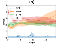
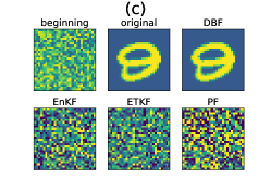
Figure 1: Results for moving MNIST experiments. Panel (a) shows the evolution of RMSE evolution for image-informed setting. Panel (b) presents RMSE for image-agnostic setting. Panel (c) compares samples of learned figures for DBF, EnKF, ETKF, and PF.

3.2 Double Pendulum

This section shows our experiments with a double pendulum system chosen for its nonlinear, chaotic nature. The pendulum comprises two weights, P1 and P2, each weighing 1 [kg], and connected by two bars, B1 and B2, each with a length of 1 [m]. The fixed end of bar B1 serves as an anchor point, while the other is affixed to weight P1. Weight P2 is connected to P1 via bar B2. See panel (a) of Figure 2 for a schematic figure.

DBF prepares a fancy latent space in addition to the physical space. We take two angles $\theta_{1},\theta_{2}$ and two angle velocities $\omega_{1},\omega_{2}$ as the physical target variables. We take the latent dimension to be 50 for DBF, VRNN, SRNN, and DKF. As the observation data, two-dimensional spatial positions of the two weights $P_{1}$ and $P_{2}$ are given with Gaussian noises. The observation operator is a combination of trigonometric functions for $\theta_{1}$ and $\theta_{2}$ and, therefore, highly nonlinear. We have experimented with $\sigma=0.1,0.3$, and $0.5$ [m]. The time step between observations is 0.03 seconds. In the emission model $p(z_{t}|h_{t})$, we assume von Mises distributions for $\theta_{1}$ and $\theta_{2}$ while Gaussians for $\omega_{1}$ and $\omega_{2}$.

We report RMSE between physical variables and the model output in Table 1. The training for KalmanNet has failed in all conditions. For DVAEs, we eliminate failed initial conditions to compute RMSE. DBF outperforms model-based and latent assimilation methods in all settings. The performance gain is critical for $\omega$, which is not inferable only from one data. Figure 2 shows an example of RMSE evolution during assimilation. DBF consistently outperforms other assimilation methodologies. The assimilation of $\omega$ proceeds during the first $\sim 20$ steps, and the excellent estimate level is maintained throughout the assimilation experiment.

A notable feature of DBF is its ability to generate samples of $z_{t}$ and evaluate the uncertainty in state estimates. To assess this, we use distributions of normalized errors $\epsilon_{norm,t,i}=(z_{t,sample,i}-z_{t,i})/\delta_{i}$, where $z_{t,i}$is the true variable of dimension $i$ at time $t$ and $\delta_{i}$ is the standard deviation of $z_{t,sample,i}$. We collect $\epsilon_{norm,t,i}$ for all steps, specifically for $i=\omega_{1}$ and $i=\omega_{2}$. We do not use $i=\theta_{1}$ and $i=\theta_{2}$ as their distributions should follow von Mises distributions. If the uncertainty estimate is accurate, $\epsilon_{norm,t,i}$ should be Gaussian with a standard deviation of one. For quantitative comparison, we compute the symmetric KL divergence (also known as Jeffreys divergence) $KL_{sym}[p,q]=(KL[p||q]+KL[q||p])/2$ between the histogram of $\epsilon_{norm,t,i}$ and a unit Gaussian. DBF shows a very low $KL_{sym}$, , indicating accurate state estimation error. Panels (c) and (d) show example histograms of $\epsilon_{norm,t,i}$ for DBF and ETKF.

Table 1: RMSE at the final step of assimilation in double pendulum experiments.

	$\sigma=0.1$		$\sigma=0.3$		$\sigma=0.5$
	$\theta$	$\omega$	$\theta$	$\omega$	$\theta$	$\omega$
DBF	0.03 $\pm$ 0.01	0.21 $\pm$ 0.04	0.05 $\pm$ 0.02	0.26 $\pm$ 0.05	0.06 $\pm$ 0.01	0.36 $\pm$ 0.04
EnKF	$0.05\pm 0.00$	$0.33\pm 0.07$	$0.14\pm 0.01$	$0.71\pm 0.09$	$0.24\pm 0.01$	$1.17\pm 0.22$
ETKF	$0.05\pm 0.01$	$0.46\pm 0.08$	$0.22\pm 0.05$	$1.41\pm 0.41$	$0.36\pm 0.08$	$2.70\pm 1.25$
PF	$0.05\pm 0.00$	$0.63\pm 0.24$	$0.21\pm 0.14$	$1.41\pm 1.30$	$0.32\pm 0.08$	$2.36\pm 2.29$
PFF	$1.27\pm 0.29$	$1.04\pm 0.15$	NA	$5.99\pm 1.09$	$5.88\pm 0.67$	NA
KNet	NA	NA	NA	NA	NA	NA
VRNN	$0.04\pm 0.01$	$0.44\pm 0.19$	$0.06\pm 0.02$	$0.35\pm 0.14$	$0.08\pm 0.04$	$0.40\pm 0.16$
SRNN	$0.05\pm 0.02$	$0.52\pm 0.18$	$0.06\pm 0.02$	$0.44\pm 0.08$	$0.08\pm 0.03$	$0.52\pm 0.22$
DKF	$0.12\pm 0.02$	$2.70\pm 0.28$	$0.17\pm 0.03$	$2.61\pm 0.74$	$0.23\pm 0.04$	$2.61\pm 0.56$

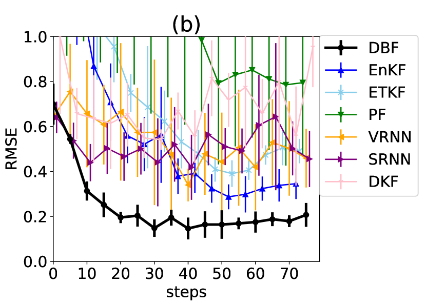
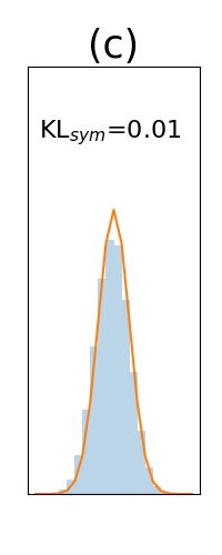
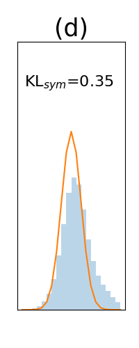
$\sigma=0.1$	KLsym
DBF	0.02
EnKF	10.2
ETKF	0.12

Figure 2: A schematic figure (panel a) and results for double pendulum experiments. Panel (b) shows the RMSE evolution during assimilation. Panels (c) and (d) show example histograms for normalized errors in DBF and ETKF outputs. The small table compares the Jeffreys divergence of normalized errors and the unit Gaussian between DBF, EnKF, and ETKF predictions.

3.3 Lorenz96

As the final experiment, we present the state estimation task within the Lorenz96 model (Lorenz, 1995). This problem serves as a pivotal test-bed for evaluating the efficacy of data-assimilation algorithms in estimating the state of a dynamical system given noisy or nonlinear observations.

The Lorenz96 model describes the behavior of a one-dimensional array of variables, each representing the evolution of a physical quantity over a spatial domain akin to an equilatitude circle. The following set of coupled ordinary differential equations governs the dynamics of the Lorenz96 model:

$$\frac{dz_{i}}{dt}=(z_{i+1}-z_{i-2})z_{i-1}-z_{i}+F,\hskip 8.53581pti=1,\ldots,N$$ (15)

where $x_{i}$ represents the variable’s value at grid point $i$, $N$ is the total number of grid points, and $F$ represents the forcing applied to the system. We have chosen $F=8$ and $N=40$.

We consider two settings for the observation operator. In the first, Gaussian noise is added to direct observations: $o_{t,j}=z_{t,j}+\epsilon,$ where $\epsilon\sim\mathcal{N}(0,\sigma^{2})$. We experiment with $\sigma=1,3,5$. In the second setting, we use a nonlinear and limited observation operator. We consider an observation operator of $o_{t,j}=min(z_{t,j}^{4},10)+\epsilon,$ where $\epsilon\sim\mathcal{N}(0,\sigma^{2})$. We experiment with $\sigma=1,3,$ and $5$. The typical dynamic range of physical values $z_{t,j}$ is $\pm 10$, and the observations are capped at ten if the absolute values of physical variables $z_{t,j}$ exceed $\sim 1.8$. All models have 80 steps as observations, with a time step between observations of 0.03. We take the latent dimension to be 800 for DBF, VRNN, SRNN, and DKF. The appendix presents details for the experimental settings and examples of Hovmöller diagrams.

Table 2: RMSE at the final step of assimilation in Lorenz96 experiments.

	direct observation			nonlinear observation
	$\sigma=1$	$\sigma=3$	$\sigma=5$	$\sigma=1$	$\sigma=3$	$\sigma=5$
DBF	$0.53\pm 0.04$	0.82 $\pm$ 0.03	1.16 $\pm$ 0.07	1.08$\pm$ 0.15	1.29 $\pm$ 0.18	1.65 $\pm$ 0.17
EnKF	$0.31\pm 0.01$	$0.83\pm 0.10$	$1.73\pm 0.12$	$4.69\pm 0.14$	$3.93\pm 0.08$	$3.81\pm 0.07$
ETKF	0.30 $\pm$ 0.01	$1.06\pm 0.15$	$2.42\pm 0.11$	$4.57\pm 0.25$	$4.28\pm 0.04$	$4.23\pm 0.07$
PF	$2.80\pm 0.04$	$3.12\pm 0.06$	$3.62\pm 0.13$	$6.05\pm 0.16$	$4.95\pm 0.12$	$4.58\pm 0.14$
PFF	$0.60\pm 0.02$	$1.00\pm 0.05$	$2.20\pm 0.09$	$3.75\pm 0.09$	$3.85\pm 0.04$	$3.83\pm 0.11$
KNet	$0.60\pm 0.02$	$1.81\pm 0.05$	$3.02\pm 0.09$	$2.97\pm 0.21$	$3.47\pm 0.17$	$3.99\pm 0.25$
VRNN	$3.67\pm 0.06$	$3.67\pm 0.06$	$3.67\pm 0.06$	$3.69\pm 0.04$	$2.51\pm 0.79$	$3.67\pm 0.06$
SRNN	$3.08\pm 0.56$	$3.63\pm 0.05$	$3.40\pm 0.29$	$3.30\pm 0.81$	$3.62\pm 0.41$	$2.96\pm 0.32$
DKF	3.70	NA	NA	NA	NA	NA

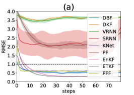
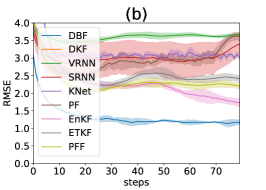
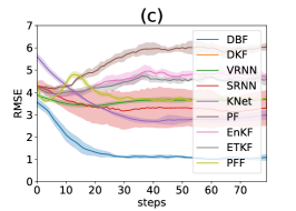
Figure 3: RMSE results for Lorenz96 experiments. Panels (a), (b) show results for direct observation with $\sigma=1$ and $\sigma=5$. Panel (c) shows results for nonlinear observation with $\sigma=1$.

Table 2 reports the assimilation performance in three different noise levels and the observation operator settings. DBF outperforms existing methods in direct observations with $\sigma=3,5$, and all noise levels in nonlinear observation cases. In the $\sigma=1$ setting with the direct observation operator, traditional algorithms (EnKF, ETKF) perform better than DBF. The excellent performances of EnKF and ETKF are due to weak non-Gaussianity in the posteriors on physical space. The low noise level allows state estimation of high accuracy. Then, the deformation of the posterior $p(z_{t+1}|o_{1:t})$ from a Gaussian is weak because the dynamics are locally linear. In that case, model-based approaches show higher performance. When the observation operator is nonlinear, performances of traditional filtering approaches crucially deteriorate. DBF consistently performs excellently compared to other methodologies.

We observe that training for DVAE methods is highly unstable. On the other hand, training for DBF is stable. The dynamics in DVAEs are expressed as RNNs, which often result in unstable training due to exploding/vanishing gradients. In DBF, the dynamics is just a matrix multiplication. If some of the eigenvalues of the dynamics matrix are significantly larger than one, the model prediction and, therefore, the loss function would explode. Figure 2 shows the histogram of absolute values of eigenvalues at the end of training, which are mostly distributed around or less than one, indicating stable training.

4 Limitation

DBF’s learning of IOO (and dynamics in nonlinear SSM cases) requires a training phase, unlike classical model-based data assimilation methods, which rely solely on perfect SSM knowledge. The reliance on training data implies potential performance challenges in scenarios when the distribution of initial conditions for test cases is unknown.

In the Lorenz96 experiment, DBF’s performance for direct observation with $\sigma=1$ falls short compared to EnKF and ETKF. In this setting, the non-Gaussianity of posteriors is weak; therefore, the approximation errors from Gaussian assumptions are minor. Hence, a model-based approach may be preferable in such cases as it fully exploits SSM knowledge without training bias.

5 Conclusion

We have proposed DBF, a novel latent assimilation method. DBF is a NN-based extension of the KF algorithm that allows nonlinear observations. A structured inference of the posterior distribution facilitates the analytic computation of the posterior. DBF shows highly competitive performances in settings where posterior distributions become highly non-Gaussian, such as nonlinear observation operators or large observation noise.

Appendix A Settings and additional results for experiments

parametrization of the dynamics matrix

We have parametrized the dynamics matrix $A$ following Lusch et al. [2018]: we consider that $h_{dim}/2$ complex eigenvalues $\lambda_{i}(0\leq i<h_{dim}/2)$ characterize $A$. Namely, $A$ is a block-diagonal matrix of $h_{dim}/2$ blocks. Each block consists of $2\times 2$ matrix, whose components are:

$$A_{block}=\exp(\rho_{i})\begin{pmatrix}\cos(\omega_{i})&-\sin(\omega_{i})\\ \sin(\omega_{i})&\cos(\omega_{i})\end{pmatrix},$$ (16)

where $\rho_{i}={\rm Re}[\lambda_{i}]$ and $\omega_{i}={\rm Im}[\lambda_{i}]$. In contrast to Lusch et al. [2018], we apply the same dynamics matrix at any positions on the latent space. We consider that this representation is sufficiently expressive as it can express any matrix on a complex number field that is diagonalizable.

Computational resources

We conduct experiments on a cluster of V100 GPUs. Each GPU has memory of 32GB.

hyperparameters for training

For all experiments we have used Adam optimizer with default parameters. Table 3 shows hyperparameters employed in our experiments. Trainings for moving MNIST and double pendulum are conducted with one GPU, while that for Lorenz96 is with eight GPUs.

Table 3: Hyperparameters for training

	lr	batch size	$h_{dim}$	$N_{data,train}$	Epochs	train time per model
moving MNIST	$10^{-3}$	64	4	16384	20	45min$\times$ 1GPU
moving MNIST image agnostic	$10^{-3}$	64	4	65536	20	3hr$\times$ 1GPU
double pendulum	$10^{-3}$	256	50	$1.0\times 10^{7}$	1	6hr$\times$ 1GPU
Lorenz96	$3\times 10^{-3}$	64	800	$2.6\times 10^{7}$	1	15hr$\times$ 8GPUs

A.1 Moving MNIST

Dataset:

A series of 2D images. The dynamic range of each pixel is 0 to 255. The training set contains 65536 initial conditions, and the test set has ten initial conditions. Both datasets are 20 steps long. The number of training data and epochs are sufficiently large so that the training mostly converges. We add a Gaussian noise of $\sigma=10$ to all the pixels. An MNIST image of the number “9” (data 5740) moves at a constant speed until it reaches the edge. Reflection occurs at the edge.

Training:

Network weight for $G_{\theta}$ is fixed during the first 10 epochs to facilitate learning of $f_{\theta}$ and the image. Then, $G_{\theta}$ is also trained for the latter 10 epochs.

Dynamics model:

Constant velocity model. We give the case for the 2D problem as an example:

$$h_{t+1}=Fh_{t}$$ (17)

$$F=\begin{pmatrix}1&0&dt&0\\ 0&1&0&dt\\ 0&0&1&0\\ 0&0&0&1\\ \end{pmatrix},z_{t}=\begin{pmatrix}x_{t}\\ y_{t}\\ v_{x_{t}}\\ v_{y_{t}}\\ \end{pmatrix},$$ (18)

and true observation model:

$$\tilde{x}_{t} = \begin{cases}(x_{t}\ \text{mod 16})&\text{if x//16 is even}\\ 9-(x_{t}\ \text{mod 16})&\text{if x//16 is odd}\\ \end{cases}\ \text{, same for $y$}$$ (19)

$$o_{t} = h(z_{t}),\mathrm{dim}(o_{t})=44\times 44\ \text{, a $28\times 28$ image is embedded at}(\tilde{x}_{t},\tilde{y}_{t}).$$ (20)

The formulation above treats the image reflection via the observation operator. It makes dynamics linear but allows multiple solutions corresponding to an observed figure. Such formulation is highly disadvantageous for EnKF, which assumes a single-peak Gaussianity on the assimilating space. To make a fair comparison, we rewrite the dynamics and observation models to allow a single solution for each figure. It significantly improves the performance of EnKF (which is reported in the main text), although the dynamics model is nonlinear due to reflection.

Network architecture:

$f_{\theta}$: Two-dimension convolutional neural networks. Below is the list of layers.

• conv1: nn.Conv2d(1, 2, kernel_size=3, stride=2, padding=1)

• conv2: nn.Conv2d(2, 4, kernel_size=3, stride=2, padding=1)

• fc1: nn.Linear($1\times 44\times 44+2\times 22\times 22+4\times 11\times 11$, 10)

• fc2: nn.Linear(10, 10)

• fc3: nn.Linear(10, 4)

The input image of size $44\times 44$ is first processed by conv1 and conv2 in parallel. Then, combine the flattened original input, conv1 output, and conv2 output to make input for fc1. The output of fc1 is then sequentially fed to fc2 and fc3. Finally, four variables for $f_{\theta}(o_{t})$ comes out. $G_{\theta}$: same as $f_{\theta}$. Here, only the diagonal components of $G_{\theta}(o_{t})$ is produced by the NN.

Table 4: List of hyperparameters for moving MNIST experiment.

parameter	value
$R$	diag[$e^{4}$]
$Q$	diag[$e^{-4}$]

Example figures:

In Figure 5, we show an example of input image and model output, and the evolution of the learned image in DBF.

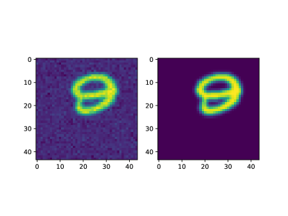
Figure 5: Left panel: an example of input data corrupted with noise, compared with the assimilation output. Right panel: evolution of the learned image embedded in dataset. Already at the end of the first epoch, DBF successfully learn the embedded image. After $20$ epochs of training, the checker-board pattern disappears and correctly determine the true image.

A.2 Double pendulum

Dataset:

2D coordinates of the positions of two weights. The training set contains 10240000 initial conditions, and the test set contains 10 initial conditions. The number of training data is sufficiently large so that the training mostly converges. For DVAE training, we have observed that some training fails due to instability. However, we keep the number of training samples as the training was successful for at least one initial condition. Both datasets are 80 steps long. The numerical integration is conducted with solve_ivp function in scipy with $\text{rtol}=10^{-2}$ and $\text{atol}=10^{-2}$.

A schematic figure explaining the problem setting is presented in panel (a) of Figure 2 in the main text. Dynamics model is described in https://matplotlib.org/stable/gallery/animation/double_pendulum.html. The length of the bars is 1 [m], and the positions of the two pendulum weights are observable with Gaussian noise of $\sigma=0.1,0.3$, or $0.5$ [m]. The observation interval is $0.03$ [s]. The task is to predict the positions of the two weights in the successive ten frames.

Network architecture:

$f_{\theta}$: A sequence of ten “linear blocks” composed of fully connected layers, layer normalizations, and skip connections. Namely, each linear block has three components:

• fc: (input dimension)$\times$ (output dimension) linear layer,

• norm: layer normalization,

• skip: skip connection.

Taking four observation variables as input, the first linear block expands it to 100 dimensions. The intermediate linear blocks keep 100 dimension variables. The final linear block shrinks 100-dimensional input to 50-dimensional output, which represent 50 variables on the latent space. The activation function is ReLU. $G_{\theta}$: same as $f_{\theta}$. $\phi_{\theta}$: inverse of $f_{\theta}$. The initial eigenvalues are randomly taken between $0$ and $10^{-2}$.

Table 5: List of hyperparameters for double pendulum experiment.

parameter	value
$R_{init}$	diag[$1$]
$Q$	diag[$e^{-6}$]
initial concentration parameter	$e^{5}$

Training:

All training variables (network weights for the IOO ($f_{\theta}$, $G_{\theta}$), the emission model operator $\phi$, eigenvalues $\lambda$ for the dynamics matrix $A$, Gaussian noise parameter $\sigma$ for angular velocity $\omega$, and the concentration parameter for Von Mises distribution used for angular coordinate $\theta$) are trained together.

Examples:

Here, we show examples for assimilated $\theta$ and $\omega$ in Figure 6. Also, we give an additional figure for the RMSE of $\theta$ for various methods.

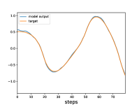
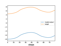
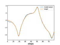
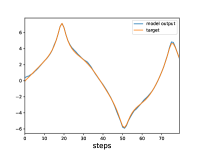
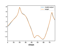
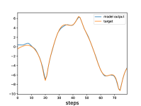
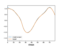
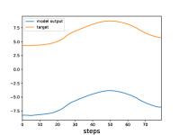
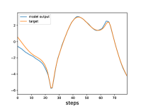
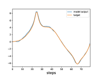
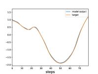
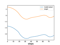
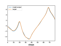
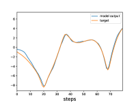
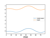
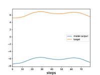
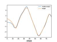
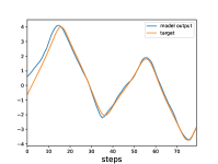
Figure 6: Results for five example data in test set. Two left columns show evolution of $\theta_{1}$ and $\theta_{2}$ (, therefore, the values are cyclic with the period of $2\pi\simeq 6.3$,) and the two right columns show $\omega_{1}$ and $\omega_{2}$.

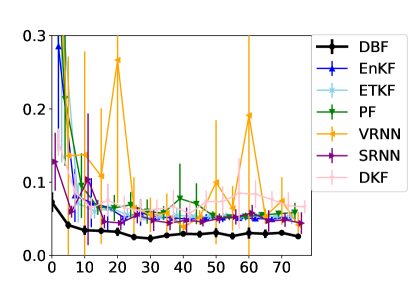
Figure 7: Assimilation results for the angle variable $\theta$. All models successfully determine the angle coordinate in spite of the strong nonlinearity in the observation (trigonometric function). Among these, performance of DBF is the best.

A.3 Lorenz96

Dataset:

Physical or observed variables on 40 grid points. The training set contains 25600000 initial conditions and the test set contains 10 initial conditions. The number of training data is sufficiently large so that the training mostly converges. The original datasets are 80 steps long. The numerical integration is conducted with solve_ivp function in scipy with $\text{rtol}=10^{-2}$ and $\text{atol}=10^{-2}$. We add Gaussian noise of $\sigma=1,3$, or $5$ onto all the measurements.

For KalmanNet, we have tried to train with 25600000 and 400000 initial conditions but the process was killed due to memory limitation. We report the results with the dataset size of 120000. For DKF, VRNN, and SRNN, we have tried to train with 25600000 conditions, but all models stop by RuntimeError in backward computation during training due to instability. To obtain results, we have reduced the number of training data to 512000. With this setting, SRNN and VRNN completed training procedure for some initial conditions.

A physical quantity $z_{j}$ is defined on each grid point $j(1\leq j\leq 40)$. A set of differential equations describes time evolution:

$$\frac{dz(t)_{j}}{dt}=(z_{j+1}-z_{j-2})z_{j-1}-z_{j}+F,(1\leq j\leq 40)$$ (21)

where the driving term $F$ is taken at $8$. The first term models the advection, and the second term models the diffusion of a physical quantity along a fixed latitude. With these parameters, the evolution of the physical quantity becomes chaotic.

Network architecture:

$f_{\theta}$: ten convolution blocks followed by a fully connected layer. Each convolution block is composed of 1D convolution, layer normalization, and skip connection:

• conv1d: nn.Conv1d( $c_{\rm in}$, $c_{\rm out}$, kernel_size=5, padding=2, padding_mode=“circular”, )

• norm: layer normalization,

• skip: skip connection.

The first convolution block has $c_{\rm in}=1$ and $c_{\rm out}=20$: it expands the input by 20 times in channel dimension. The following eight layers keep 20 channels. Finally, the 20 channels and 40 physical dimensions are flattened to 800 dimension variables, and it is fed to a fully-connected layer of $800\times 800$. For all layers, the activation function is ReLU. $G_{\theta}$: same as $f_{\theta}$. $\phi_{\theta}$: inverse of $f_{\theta}$.

Table 6: List of hyperparameters for Lorenz96 experiment.

parameter	value
$R_{init}$	diag[$1$]
$Q$	diag[$e^{-8}$]

Training:

All training variables (network weights for the IOO ($f_{\theta}$, $G_{\theta}$), the emission model operator $\phi$, eigenvalues $\lambda$ for the dynamics matrix $A$, and the Gaussian noise parameter $\sigma$) are trained together.

Examples:

Here, we show an example figure for assimilation experiment with DBF.

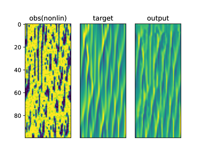
Figure 8: An example of assimilation output in the experiment with nonlinear observation operator. The observation is not very informative due to low threshold for saturation in the observation operator ($o_{t,j}=min(z_{t,j}^{4},10)+\epsilon,$, all cells with $z_{t,j}>1.8$ are just observed as $10+\epsilon$). In the first 20 steps, the model output resembles little with the target. However, as the step proceeds, model output begins to capture features of the true state. Even with such a poor observation operator, DBF finds a latent space representation that captures the evolution of the true state.

Appendix B training stability

We observe that the training of our proposed method is stable compared to RNN-based models. Figure 9 shows the evolution of the real parts of eigenvalues. Although we do not impose constraints on the real parts of eigenvalues, the values only marginally exceed one. Therefore, long-time dynamics is stable during training.

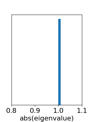
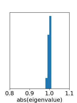
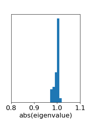
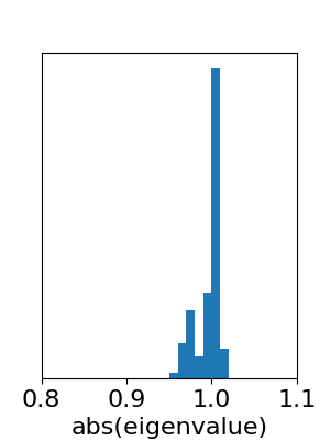
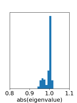
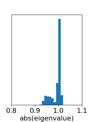
Figure 9: Evolution of histograms for the real parts of 800 complex eigenvalues in Lorenz96 experiment. Initially, eigenvalues are taken as one. As the model learns the dynamics, eigenvalues lower than 1.0 appear. However, the largest eigenvalue $\lambda_{max}$ mostly remains less than 1.02.

Appendix C Broader Impacts

Our methodology helps estimate the true state better from noisy observations. It will have positive impacts on various scientific domains that include state estimation processes from noisy observations, e.g., weather forecasting. It should not have negative societal impact unless intentionally misinterpret or misuse the results.

References

- Alfonzo and Oliver (2020) Miguel Alfonzo and Dean S. Oliver. Seismic data assimilation with an imperfect model. Computational Geosciences, 24(2):889–905, 2020. Marine Environmental Monitoring and Prediction.
- Andrychowicz et al. (2023) Marcin Andrychowicz, Lasse Espeholt, Di Li, Samier Merchant, Alexander Merose, Fred Zyda, Shreya Agrawal, and Nal Kalchbrenner. Deep learning for day forecasts from sparse observations. ArXiv, abs/2306.06079, 2023. URL https://api.semanticscholar.org/CorpusID:259129311.
- Awal et al. (2023) Md Abdul Awal, Md Abu Rumman Refat, Feroza Naznin, and Md Zahidul Islam. A particle filter based visual object tracking: A systematic review of current trends and research challenges. International Journal of Advanced Computer Science and Applications, 14(11), 2023. doi: 10.14569/IJACSA.2023.01411131. URL http://dx.doi.org/10.14569/IJACSA.2023.01411131.
- Azencot et al. (2020) Omri Azencot, N. Benjamin Erichson, Vanessa Lin, and Michael Mahoney. Forecasting sequential data using consistent koopman autoencoders. In Hal Daumé III and Aarti Singh, editors, Proceedings of the 37th International Conference on Machine Learning, volume 119 of Proceedings of Machine Learning Research, pages 475–485. PMLR, 13–18 Jul 2020. URL https://proceedings.mlr.press/v119/azencot20a.html.
- Bach and Ghil (2023) Eviatar Bach and Michael Ghil. A multi-model ensemble kalman filter for data assimilation and forecasting. Journal of Advances in Modeling Earth Systems, 15(1):e2022MS003123, 2023. doi: https://doi.org/10.1029/2022MS003123. URL https://agupubs.onlinelibrary.wiley.com/doi/abs/10.1029/2022MS003123. e2022MS003123 2022MS003123.
- Bishop et al. (2001) Craig H. Bishop, Brian J. Etherton, and Sharanya J. Majumdar. Adaptive Sampling with the Ensemble Transform Kalman Filter. Part I: Theoretical Aspects. Mon. Wea. Rev., 129(3):420–436, March 2001. ISSN 0027-0644, 1520-0493. doi: 10.1175/1520-0493(2001)129<0420:ASWTET>2.0.CO;2. URL http://journals.ametsoc.org/doi/10.1175/1520-0493(2001)129<0420:ASWTET>2.0.CO;2.
- Daum and Huang (2007) Fred Daum and Jim Huang. Nonlinear filters with log-homotopy. In Oliver E. Drummond and Richard D. Teichgraeber, editors, Signal and Data Processing of Small Targets 2007, volume 6699, page 669918. International Society for Optics and Photonics, SPIE, 2007. doi: 10.1117/12.725684. URL https://doi.org/10.1117/12.725684.
- Evensen (1994) Geir Evensen. Sequential data assimilation with a nonlinear quasi-geostrophic model using Monte Carlo methods to forecast error statistics. Journal of Geophysical Research: Oceans, 99(C5):10143–10162, 1994. ISSN 2156-2202. doi: 10.1029/94JC00572. URL https://onlinelibrary.wiley.com/doi/abs/10.1029/94JC00572. _eprint: https://onlinelibrary.wiley.com/doi/pdf/10.1029/94JC00572.
- Frerix et al. (2021) Thomas Frerix, Dmitrii Kochkov, Jamie Smith, Daniel Cremers, Michael Brenner, and Stephan Hoyer. Variational Data Assimilation with a Learned Inverse Observation Operator. In Proceedings of the 38th International Conference on Machine Learning, pages 3449–3458. PMLR, July 2021. URL https://proceedings.mlr.press/v139/frerix21a.html. ISSN: 2640-3498.
- Girin et al. (2021) Laurent Girin, Simon Leglaive, Xiaoyu Bie, Julien Diard, Thomas Hueber, and Xavier Alameda-Pineda. Dynamical variational autoencoders: A comprehensive review. Foundations and Trends® in Machine Learning, 15(1-2):1–175, 2021. ISSN 1935-8237. doi: 10.1561/2200000089. URL http://dx.doi.org/10.1561/2200000089.
- Gu and Dao (2023) Albert Gu and Tri Dao. Mamba: Linear-time sequence modeling with selective state spaces. arXiv preprint arXiv:2312.00752, 2023.
- Gu et al. (2022) Albert Gu, Karan Goel, and Christopher Re. Efficiently modeling long sequences with structured state spaces. In International Conference on Learning Representations, 2022. URL https://openreview.net/forum?id=uYLFoz1vlAC.
- Hu and van Leeuwen (2021) Chih-Chi Hu and Peter Jan van Leeuwen. A particle flow filter for high-dimensional system applications. Quarterly Journal of the Royal Meteorological Society, 147(737):2352–2374, 2021. doi: https://doi.org/10.1002/qj.4028. URL https://rmets.onlinelibrary.wiley.com/doi/abs/10.1002/qj.4028.
- Hunt et al. (2007) Brian R. Hunt, Eric J. Kostelich, and Istvan Szunyogh. Efficient data assimilation for spatiotemporal chaos: A local ensemble transform kalman filter. Physica D: Nonlinear Phenomena, 230(1):112–126, 2007. ISSN 0167-2789. doi: https://doi.org/10.1016/j.physd.2006.11.008. URL https://www.sciencedirect.com/science/article/pii/S0167278906004647. Data Assimilation.
- Kalman (1960) R. E. Kalman. A New Approach to Linear Filtering and Prediction Problems. Journal of Basic Engineering, 82(1):35–45, 03 1960. ISSN 0021-9223. doi: 10.1115/1.3662552. URL https://doi.org/10.1115/1.3662552.
- Koopman (1931) B. O. Koopman. Hamiltonian systems and transformation in hilbert space. Proceedings of the National Academy of Sciences, 17(5):315–318, 1931. doi: 10.1073/pnas.17.5.315. URL https://www.pnas.org/doi/abs/10.1073/pnas.17.5.315.
- Larsen et al. (2007) J. Larsen, J.L. Høyer, and J. She. Validation of a hybrid optimal interpolation and kalman filter scheme for sea surface temperature assimilation. Journal of Marine Systems, 65(1):122–133, 2007. ISSN 0924-7963. doi: https://doi.org/10.1016/j.jmarsys.2005.09.013. URL https://www.sciencedirect.com/science/article/pii/S0924796306002880. Marine Environmental Monitoring and Prediction.
- Lippe et al. (2023) Phillip Lippe, Bastiaan S. Veeling, Paris Perdikaris, Richard E Turner, and Johannes Brandstetter. PDE-Refiner: Achieving Accurate Long Rollouts with Temporal Neural PDE Solvers. In Thirty-seventh Conference on Neural Information Processing Systems, 2023. URL https://openreview.net/forum?id=Qv6468llWS.
- Lorenc (2003) Andrew C. Lorenc. Modelling of error covariances by 4d-var data assimilation. Quarterly Journal of the Royal Meteorological Society, 129(595):3167–3182, 2003. doi: https://doi.org/10.1256/qj.02.131. URL https://rmets.onlinelibrary.wiley.com/doi/abs/10.1256/qj.02.131.
- Lorenz (1995) E.N. Lorenz. Predictability: a problem partly solved. PhD thesis, Shinfield Park, Reading, 1995 1995.
- Lusch et al. (2018) Bethany Lusch, J. Nathan Kutz, and Steven L. Brunton. Deep learning for universal linear embeddings of nonlinear dynamics. Nature Communications, 9:4950, November 2018. doi: 10.1038/s41467-018-07210-0.
- Revach et al. (2022) Guy Revach, Nir Shlezinger, Xiaoyong Ni, Adrià López Escoriza, Ruud J. G. van Sloun, and Yonina C. Eldar. Kalmannet: Neural network aided kalman filtering for partially known dynamics. IEEE Transactions on Signal Processing, 70:1532–1547, 2022. doi: 10.1109/TSP.2022.3158588.
- Takeishi et al. (2017) Naoya Takeishi, Yoshinobu Kawahara, and Takehisa Yairi. Learning koopman invariant subspaces for dynamic mode decomposition. In I. Guyon, U. Von Luxburg, S. Bengio, H. Wallach, R. Fergus, S. Vishwanathan, and R. Garnett, editors, Advances in Neural Information Processing Systems, volume 30. Curran Associates, Inc., 2017. URL https://proceedings.neurips.cc/paper_files/paper/2017/file/3a835d3215755c435ef4fe9965a3f2a0-Paper.pdf.
- Zhou et al. (2023) Linqi Zhou, Michael Poli, Winnie Xu, Stefano Massaroli, and Stefano Ermon. Deep latent state space models for time-series generation. In Andreas Krause, Emma Brunskill, Kyunghyun Cho, Barbara Engelhardt, Sivan Sabato, and Jonathan Scarlett, editors, International Conference on Machine Learning, ICML 2023, 23-29 July 2023, Honolulu, Hawaii, USA, volume 202 of Proceedings of Machine Learning Research, pages 42625–42643. PMLR, 2023. URL https://proceedings.mlr.press/v202/zhou23i.html.