Adapting Differentially Private Synthetic Data to Relational Databases

Abstract

Existing differentially private (DP) synthetic data generation mechanisms typically assume a single-source table. In practice, data is often distributed across multiple tables with relationships across tables. In this paper, we introduce the first-of-its-kind algorithm that can be combined with any existing DP mechanisms to generate synthetic relational databases. Our algorithm iteratively refines the relationship between individual synthetic tables to minimize their approximation errors in terms of low-order marginal distributions while maintaining referential integrity. Finally, we provide both DP and theoretical utility guarantees for our algorithm.

1 Introduction

Relational databases play a pivotal role in modern information systems and business operations due to their efficiency in managing structured data [39]. According to a Kaggle survey [23], 65.5% of users worked extensively with relational data. Additionally, the majority of leading database management systems (e.g., MySQL and Oracle) are built on relational database principles [35]. These systems organize data into multiple tables, each representing a specific entity, and the relationships between tables delineate the connections between these entities. However, the widespread use of relational databases also carries a significant risk of privacy leakage. For example, if a single table suffers from a privacy breach, all other tables containing sensitive information can be exposed, as they are interconnected and share relationships. Moreover, deleting data in a relational database can be complex, and incomplete deletion can leave traces of data, which can potentially be accessed and reconstructed by attackers.

Today, differential privacy (DP) stands as the de facto standard for privacy protection. There is a growing body of research focused on applying DP to generate private synthetic data [see, e.g., 36, 31, 27, 41]. This effort enables data curators to share (synthetic) data while ensuring the privacy of individuals’ personal information within the original dataset. In return, they can harness advanced machine learning techniques employed by end-users trained on the synthetic data. Numerous studies have provided evidence that state-of-the-art (SOTA) DP synthetic data effectively preserves both the statistical properties of the original data and the high performance of downstream predictive models trained on these synthetic datasets when deployed on the original data [45, 51]. However, all existing works assume a single-source database (with a few exceptions discussed in Related Work). It motivates the central question we aim to tackle in this paper:

Can we adapt existing DP synthetic data generation algorithms to relational databases while preserving their referential integrity?

The conventional approach—flattening relational databases into a single master table, generating a synthetic master table, and dividing it into separate databases—presents several challenges. To illustrate, consider education data as an example, with two tables (student and teacher information) linked by students’ enrollment in a teacher’s course. First, flattening often introduces numerous null values, complicating the differentiation between missing and intentionally null data. If a teacher isn’t teaching, student information in the master table will show up as null, even if the original tables had none. Second, flattening creates scalability and redundancy issues. Records in the master table often contain a high number of features, leading to longer running times for SOTA DP synthetic data generation algorithms as features increase [e.g., 32, 31, 50, 1]. Moreover, records from the original tables can be duplicated across entries, increasing redundancy and storage demand. Finally, breaking down a synthetic master table may disrupt relationships when shared feature values are involved. For instance, if the master table contains two courses with students sharing identical demographic data, it’s unclear if they’re the same student or different individuals with matching details.

Our goal is to introduce the first-of-its-kind algorithm that can generate synthetic relational databases while preserving the privacy, statistical properties, and referential integrity of the original data. For this purpose, we first discuss DP in relational databases, extend the definition of $k$-way marginal queries [46, 36] to relational databases, and articulate the requirements of referential integrity (Section 2). The main technical contribution is introducing an iterative algorithm that effectively learns the relationship between various tables (Section 3). At each iteration, the algorithm identifies a subset of $k$-way marginal queries with the highest approximation errors and then refines the relational synthetic database to minimize these errors. Notably, our algorithm avoids the need to flatten relational databases into a master table; instead, it only requires querying the relational databases to compute low-order marginal distributions, which can be done using SQL aggregate functions. Consequently, we can leverage any off-the-shelf DP mechanisms to generate synthetic data for individual tables and apply our algorithm to establish their inter-table relationship. We analyze our algorithm theoretically, establishing both DP and utility guarantees.

Existing literature on synthetic relational data generation, even without DP guarantees, remains limited [29, 34, 53, 14, 10, 54].

In summary, our contributions include:

• Presenting a pioneering study on privacy-preserving synthetic data generation in relational databases.

• Introducing an iterative algorithm that establishes relationships between synthetic tables while preserving statistical properties and referential integrity.

• Developing a model-agnostic approach that integrates with any DP synthetic data algorithm, offering both privacy and utility guarantees.

Related Work

Privacy-preserving synthetic data generation is an active research topic [see e.g., 5, 47, 6, 11, 16, 37, 51]. For example, a line of work considered learning probabilistic graphical models [55, 30, 31] or generative adversarial networks [52, 2, 22, 44, 33, 3] with DP guarantees and generating synthetic data by sampling from these models. Another line of work proposed to iteratively refine synthetic data to minimize its approximation error on a pre-selected set of workload queries [18, 15, 32, 27, 26, 49, 1, 50, 28]. They only focused on a single-source dataset without considering relational database. The only exceptions are [53, 10]. [10] used graphical models for generating DP synthetic data, incorporating latent variables to capture the primal-foreign-key relationship. However, their method is limited to one-to-many relationships while our method can handle relationships of any type. A more closely related work is [53], which can produce multiple tables with many-to-many relationships by leveraging tools from random graph theory and representation learning. However, their method required using DP-SGD to optimize their generative models for each table generation, whereas our method can seamlessly integrate with any existing DP mechanisms for synthetic table generation. This versatility is essential, particularly as marginal-based and workload-based mechanisms often produce higher-quality synthetic tabular data than DP-SGD-based mechanisms [45, 31, 51]. Finally, some research explored DP in relational database systems, primarily focusing on releasing statistical queries [see e.g., 20, 21, 24]. In contrast, our emphasis is on releasing a synthetic copy of the relational database, extending the scope of privacy-preserving data generation methods to a more practical and general setting.

Another line of work focused on the release of DP synthetic graphs [25, 56, 13, 48, 17, 4, 38, 19] with the goal of maintaining essential graph properties (e.g., connectivity, degree distribution, and cut approximation). While a relational database can often be represented as a multipartite graph (see Section 2.1), applying these existing approaches to generate synthetic relational databases encounters various challenges. First, these methods often assume that the vertex set of both real and synthetic graphs is common, learning the edge set through DP mechanisms. In our scenario, however, the vertex sets (representing records) of real and synthetic databases differ, requiring privacy preservation for both the vertex set and the edge set. Additionally, existing approaches focus on preserving graph properties, whereas our objective extends to preserve both graph properties (i.e., relationships between different tables) and statistical properties of relational databases.

2 Preliminaries and Problem Formulation

We introduce notation, represent relational databases through bipartite graphs, review differential privacy and its properties, and provide an overview of our problem formulation.

2.1 Bipartite Graph and Relational Database

To simplify our presentation, we assume that the relational database $\mathcal{B}$ consists of only two tables $\mathcal{D}_{1}$ and $\mathcal{D}_{2}$ (e.g., student and teacher information), each having $n_{1}$ and $n_{2}$ rows. The relationship between tables is typically defined through primary and foreign keys. A primary key is a column in a table serving as a unique identifier for each row. A foreign key is a column that establishes a relationship between tables by referencing the primary key of a different table.

We represent the relational database as a bipartite graph $\mathcal{B}=(\mathcal{D}_{1},\mathcal{D}_{2},\bm{B})$ where each record corresponds to a node; the two tables define two distinct sets of nodes; and the relationships between the tables are depicted as edges connecting these nodes. We represent the edges using a bi-adjacency matrix, denoted as $\bm{B}\in\{0,1\}^{n_{1}\times n_{2}}$, where $B_{i,j}=1$ iff the i-th record from table $\mathcal{D}_{1}$ is connected to the j-th record from table $\mathcal{D}_{2}$ (e.g. if the i-th student is enrolled in the j-th teacher’s course). For each record $\bm{x}$, we represent its degree as the total number of records from the other table connected to $\bm{x}$, denoted by $\deg(\bm{x})$. Finally, we assume the degree of each record is upper bounded by a constant $d_{\max}$.

2.2 Differential Privacy

We first recall the definition of differential privacy (DP) [12].

Definition 1.

A randomized mechanism $\mathcal{M}$ that takes a relational database as input and returns an output from a set $\mathcal{R}$ satisfies $(\varepsilon,\delta)$-differential privacy, if for any adjacent relational databases $\mathcal{B}$ and $\mathcal{B}^{\prime}$ and all possible subsets $\mathcal{O}$ of $\mathcal{R}$, we have

$$\Pr(\mathcal{M}(\mathcal{B})\in\mathcal{O})\leq e^{\varepsilon}\Pr(\mathcal{M}(\mathcal{B}^{\prime})\in\mathcal{O})+\delta.$$ (1)

We consider two relational databases $\mathcal{B}$ and $\mathcal{B}^{\prime}$ adjacent if $\mathcal{B}^{\prime}$ can be obtained from $\mathcal{B}$ by selecting a table, modifying the values of a single row within this table, and changing all relationships associated with this row.

DP plays a pivotal role in answering statistical queries, with two distinct categories to be considered for relational databases. The first class involves queries pertaining to a single table, say table $\mathcal{D}_{1}$. In the context of a student-teacher database, an example would be a query about whether a student is a freshman. If we denote the data domain of table $\mathcal{D}_{1}$ by $\mathcal{X}_{1}$, a statistical query can be represented by a function $q:\mathcal{X}_{1}\to\{0,1\}$ and its average over a database is denoted as $q(\mathcal{B})\triangleq\frac{1}{n_{1}}\sum_{\bm{x}\in\mathcal{D}_{1}}q(\bm{x})$. The second class includes cross-table queries, such as whether a teacher and a student belong to the same department. Analogously, these queries are represented by a function $q:\mathcal{X}_{1}\times\mathcal{X}_{2}\to\{0,1\}$. We denote the average of their values over a database by $q(\mathcal{B})\triangleq\frac{1}{\bm{1}^{T}\cdot\operatorname{vec}(\bm{B})}\sum q(\bm{x}_{i},\bm{x}_{j})$ where the sum is over $(\bm{x}_{i},\bm{x}_{j})\in\mathcal{D}_{1}\times\mathcal{D}_{2}$ s.t. $B_{i,j}=1$ and $\operatorname{vec}(\cdot)$ converts a matrix into a vector. When $(\mathcal{D}_{1},\mathcal{D}_{2})$ are clear from the context, we also express the query in terms of the bi-adjacency matrix $\bm{B}$.

2.3 Problem Formulation

Our goal is to generate a privacy-preserving synthetic database $\mathcal{B}_{\text{syn}}=(\mathcal{D}_{1}^{\text{syn}},\mathcal{D}_{2}^{\text{syn}},\bm{B}^{\text{syn}})$ that preserves both statistical properties and referential integrity of the original relational database. In terms of statistical properties, our aim is to ensure that the marginal distributions of subsets of features in the synthetic data closely align with those of the real data. To achieve this, we revisit the definition of $k$-way marginal query and extend it to suit relational databases.

Definition 2.

Suppose the domain of table $\mathcal{D}_{i}$ has $d_{i}$ categorical features: $\mathcal{X}_{i}=\mathcal{X}_{i,1}\times\cdots\mathcal{X}_{i,d_{i}}$. We define a $k$-way workload as a subset of $k$ features: $\mathcal{S}\subseteq[d_{1}]$ (or $\mathcal{S}\subseteq[d_{2}]$) with $|\mathcal{S}|=k$. Additionally, given a reference value $\bm{y}$, we define a (single-table) $k$-way marginal query as

$$q_{\mathcal{S},\bm{y}}(\bm{x})\triangleq\prod_{j\in\mathcal{S}}\mathbb{I}({x_{j}=y_{j}})\quad\text{for }\bm{x}\in\mathcal{X}_{1}\ (\text{or }\mathcal{X}_{2})$$ (2)

where $\mathbb{I}$ is an indicator function. Analogously, we define a (cross-table) $k$-way workload as $\mathcal{S}_{1}\times\mathcal{S}_{2}\subseteq[d_{1}]\times[d_{2}]$ with $|\mathcal{S}_{1}|+|\mathcal{S}_{2}|=k$, $0<|\mathcal{S}_{1}|<k$; additionally, given a reference value $(\bm{y}_{1},\bm{y}_{2})$, we define a (cross-table) $k$-way marginal query $q_{(\mathcal{S}_{1},\mathcal{S}_{2}),(\bm{y}_{1},\bm{y}_{2})}(\bm{x}_{1},\bm{x}_{2})$ is defined as

$$\prod_{(j_{1},j_{2})\in\mathcal{S}}\mathbb{I}({(x_{1,j_{1}},x_{2,j_{2}})=(y_{1,j_{1}},y_{2,j_{2}})})$$

for $(\bm{x}_{1},\bm{x}_{2})\in\mathcal{X}_{1}\times\mathcal{X}_{2}$. We denote the set of all (cross-table) $k$-way marginal workloads by $\mathcal{W}_{\text{cross},k}$ and their associated queries by $\mathcal{Q}_{\text{cross},k}$.

In maintaining referential integrity, we use a linking table to establish relationships. It is designed to store the IDs of synthetic tables: the entry $(i,j)$ is included in this table if $\bm{B}_{i,j}^{\text{syn}}=1$. Moreover, when the original database exhibits a one-to-many relationship (i.e., a record in the parent table $\mathcal{D}_{1}$ can be related to one or more records in $\mathcal{D}_{2}$, but a record in the child $\mathcal{D}_{2}$ can be related to only one record in $\mathcal{D}_{1}$) or one-to-one relationship, we expect the synthetic database to preserve this relationship. Finally, in the case of a one-to-many relationship in the original database, we ensure there are no orphaned rows in the synthetic database. Specifically, we impose the requirement that each record in the child table $\mathcal{D}_{2}^{\text{syn}}$ connects to a record in the parent table $\mathcal{D}_{1}^{\text{syn}}$ (although records in the parent table are permitted to have no associated child records).

3 Main Results

We present our main algorithm (Algorithm 1) for generating privacy-preserving synthetic relational databases. This algorithm can be combined with any existing single-source DP synthetic data mechanisms, adapting them to the relational database context by establishing relationships among individual synthetic tables. Specifically, it learns a bi-adjacency matrix by minimizing approximation errors in cross-table $k$-way marginal queries compared to the original data. Given the inherent large size of the query class, our algorithm employs an iterative approach to identify the queries with the highest approximation errors and refine the bi-adjacency matrix to reduce these errors. Our algorithm is designed for efficiency and scalability, making it well-suited for high-dimensional data. It also ensures referential integrity in the generated synthetic relational data. We end this section by establishing rigorous utility and DP guarantees for our algorithm.

We first create individual synthetic tables $\mathcal{D}_{i}^{\text{syn}}$ by applying any DP mechanisms via black-box access. Our main technical contribution lies in establishing connections among these synthetic tables by constructing a bi-adjacency matrix $\bm{B}$ that links them. We learn this matrix by aligning the cross-table $k$-way marginal queries between the synthetic and original databases. The key observation is that each of these marginal queries can be written as a (fractional) linear function of the bi-adjacency matrix. We formalize this observation in the following lemma.

Lemma 1.

For a relational database $(\mathcal{D}_{1},\mathcal{D}_{2},\bm{B})$ and any $k$-way cross-table query $q_{(\mathcal{S}_{1},\mathcal{S}_{2}),(\bm{y}_{1},\bm{y}_{2})}$, let $\bm{1}_{(\mathcal{S}_{1},\bm{y}_{1})}\in\{0,1\}^{n_{1}}$ denote an indicator vector whose i-th element equals $1$ iff the $i$-th record in $\mathcal{D}_{1}$ satisfies $x_{i,j}=y_{1,j}$ for all $j\in\mathcal{S}_{1}$. Let $\bm{q}_{(\mathcal{S}_{1},\mathcal{S}_{2}),(\bm{y}_{1},\bm{y}_{2})}=\operatorname{vec}(\bm{1}_{(\mathcal{S}_{1},\bm{y}_{1})}\otimes\bm{1}_{(\mathcal{S}_{2},\bm{y}_{2})})$. Then we have:

$$q_{(\mathcal{S}_{1},\mathcal{S}_{2}),(\bm{y}_{1},\bm{y}_{2})}(\bm{B})=\frac{\bm{q}^{T}_{(\mathcal{S}_{1},\mathcal{S}_{2}),(\bm{y}_{1},\bm{y}_{2})}\cdot\operatorname{vec}(\bm{B})}{\bm{1}^{T}\cdot\operatorname{vec}(\bm{B})}.$$ (3)

Based on the above lemma, we write the cross-table query and its corresponding vector $\bm{q}_{(\mathcal{S}_{1},\mathcal{S}_{2}),(\bm{y}_{1},\bm{y}_{2})}$ interchangeably. We learn the bi-adjacency matrix of the synthetic database by solving the following optimization:

$$\min_{\begin{subarray}{c}\bm{b}^{\text{syn}}\in\{0,1\}^{n^{\text{syn}}_{1}\cdot n^{\text{syn}}_{2}}\\ \bm{1}^{T}\bm{b}^{\text{syn}}=m^{\text{syn}}\end{subarray}}\max_{\bm{q}\in\mathcal{Q}_{\text{cross},k}}\left|\frac{1}{m^{\text{syn}}}\bm{q}^{T}\bm{b}^{\text{syn}}-a\right|.$$ (4)

where $\bm{b}^{\text{syn}}=\operatorname{vec}(\bm{B}^{\text{syn}})$ and $a$ is the query value computed from the original real data. Since the minimization over $\bm{b}^{\text{syn}}$ in (4) is a combinatorial optimization, which is inherently challenging to solve, we solve a relaxed problem by allowing $\bm{b}^{\text{syn}}\in[0,1]^{n^{\text{syn}}_{1}\cdot n^{\text{syn}}_{2}}$ and use a randomized rounding algorithm to convert the obtained values back into integer values.

We present an iterative algorithm for solving the above optimization with DP guarantees. At each iteration, we apply the exponential mechanism to identify cross-table $k$-way workloads whose corresponding queries have the highest approximation errors between synthetic and real databases. Then we add isotropic Gaussian noise to their query values and update the (vectorized) bi-adjacency matrix $\bm{b}^{\text{syn}}$ to reduce these approximation errors. Specifically, at iteration $t$, we stack all the queries reported so far into a matrix $\hat{\bm{Q}}$ and let their noisy answers be a vector $\hat{\bm{a}}$. To update $\bm{b}^{\text{syn}}$, we use a mirror descent update with negative entropy mirror [8] to solve the following bounded-variable least-squares problem [42, 7] (see Appendix B for details):

$$\min_{\begin{subarray}{c}\bm{b}\in[0,1]^{n^{\text{syn}}_{1}\cdot n^{\text{syn}}_{2}}\\ \bm{1}^{T}\bm{b}=m^{\text{syn}}\end{subarray}}\left\|\frac{1}{m^{\text{syn}}}\hat{\bm{Q}}\bm{b}-\hat{\bm{a}}\right\|_{2}^{2}.$$ (5)

Suppose $\bm{b}^{\text{syn}}$ is the output from the preceding procedure, which we reshape into a matrix. Next, we introduce a randomized rounding algorithm to convert $\bm{b}^{\text{syn}}$ into $\{0,1\}^{n^{\text{syn}}_{1}\times n^{\text{syn}}_{2}}$ for defining the relationship between synthetic tables. Given that $\bm{b}^{\text{syn}}/m^{\text{syn}}$ forms a valid probability distribution over the domain $[n^{\text{syn}}_{1}]\times[n^{\text{syn}}_{2}]$, we sample random values from this distribution, rejecting those that have already been selected. We iterate this process until we obtain $m^{\text{syn}}$ distinct random values. These values correspond to the indices of the bi-adjacency matrix $\bm{B}^{\text{syn}}$ whose value is $1$.

We outline the above procedure in Algorithm 1 and provide additional details, including our privacy budget tracking, hyper-parameters, the updating rule for mirror descent, and discretization strategy, in Appendix B. We explore strategies for ensuring the scalability of our algorithm for synthesizing large-scale relational databases in Appendix E. We show how our above procedure can be adapted if the original database has a one-to-many relationship in Appendix D. We remark that iterative algorithms are a standard technique for query releasing in the DP literature [see 17, 18, 27, 1, 32, for examples in synthetic data/graph generation] and we extend its applications to establish relationships between synthetic tables. We end this section by establishing DP and utility guarantees for our algorithm.

Algorithm 1 Adapting DP mechanisms to generate relational synthetic data.

Input: private relational database $\mathcal{B}=(\mathcal{D}_{1},\mathcal{D}_{2},\bm{B})$; privacy budget $(\varepsilon_{\text{rel}},\delta_{\text{rel}})$; individual synthetic tables $\mathcal{D}_{1}^{\text{syn}}$, $\mathcal{D}_{2}^{\text{syn}}$; workloads per iteration $K$; number of iterations $T$; number of relationship in synthetic tables: $m^{\text{syn}}$

Initialize: $\hat{\bm{Q}}=\emptyset,\hat{\bm{a}}=\emptyset$, $\bm{b}^{\text{syn}}\in[0,1]^{n_{1}^{\text{syn}}\cdot n_{2}^{\text{syn}}}$

for $t=1,\cdots,T$ do

     Select $K$ workloads via the exponential mechanism

     Append the queries from the new workloads to $\hat{\bm{Q}}$.

     Add noise to the new query answers and append them to $\hat{\bm{a}}$.

     Solve $\bm{b}^{\text{syn}}={\arg\min}_{\begin{subarray}{c}\bm{b}\in[0,1]^{n_{1}^{\text{syn}}\cdot n_{2}^{\text{syn}}}\\ \bm{1}^{T}\bm{b}=m^{\text{syn}}\end{subarray}}\lVert\frac{1}{m^{\text{syn}}}\hat{\bm{Q}}\bm{b}-\hat{\bm{a}}\rVert_{2}^{2}$

     $\bm{B}^{\text{syn}}=\operatorname{RandomizedRounding}(\bm{b}^{\text{syn}}.\text{reshape}(n_{1}^{\text{syn}},n_{2}^{\text{syn}}))$

end for

Output: $\mathcal{B}^{\text{syn}}=(\mathcal{D}^{\text{syn}}_{1},\mathcal{D}^{\text{syn}}_{2},\bm{B}^{\text{syn}})$

Theorem 1.

Suppose we use any DP mechanism with privacy budgets $(\varepsilon_{1},\delta_{1})$ and $(\varepsilon_{2},\delta_{2})$ to generate individual synthetic tables, respectively. Then we apply Algorithm  1 with privacy budget $(\varepsilon_{\text{rel}},\delta_{\text{rel}})$ to build their relationship. The synthetic relational database satisfies $(\varepsilon_{1}+\varepsilon_{2}+\varepsilon_{\text{rel}},\delta_{1}+\delta_{2}+\delta_{\text{rel}})$-DP.

Next, we present a utility theorem that provides an upper bound on the approximation error of cross-table queries using synthetic relational data generated by Algorithm 1.

Theorem 2.

Let $\bm{b}^{\text{syn}}=\operatorname{vec}(\bm{B}^{\text{syn}})$ be the output of Algorithm 1 (without randomized rounding) for a single iteration across all $k$-way workloads, while $\bm{b}^{*}=\operatorname{vec}(\bm{B}^{*})$ denotes the optimal bi-adjacency matrix achievable for the synthetic individual tables without any privacy constraints. We stack all the query vectors as matrices $\bm{Q}$ and $\hat{\bm{Q}}$ for the original and synthetic tables, respectively. Let $\bm{a}$ be the true answers of all queries computed from the original database. With high probability,

$$\frac{\left\|\frac{1}{m^{\text{syn}}}\hat{\bm{Q}}\bm{b}^{\text{syn}}-\bm{a}\right\|_{2}^{2}}{|\mathcal{W}_{\text{cross},k}|}\leq 8\frac{\left\|\frac{1}{m^{\text{syn}}}\hat{\bm{Q}}\bm{b}^{*}-\bm{a}\right\|_{2}^{2}}{|\mathcal{W}_{\text{cross},k}|}+O\left(\frac{d_{\text{max}}}{m\sqrt{\rho_{\text{rel}}}}\right).$$

where $\rho_{\text{rel}}=\left(\sqrt{\varepsilon_{\text{rel}}+\operatorname{log}\frac{1}{\delta_{\text{rel}}}}-\sqrt{\operatorname{log}\frac{1}{\delta_{\text{rel}}}}\right)^{2}$ and we ignore logarithmic terms.

The theorem above bounds the per-workload squared error in estimating cross-table queries using synthetic data from Algorithm 1. This upper bound consists of the optimal error without privacy constraints and an additional error term. The optimal error depends on the quality of the individual synthetic tables and the selected privacy mechanism. If the synthetic tables matched the original, the optimal error would be zero. The additional error term is influenced by three factors: $m$ (number of relationships in the original database), $d_{\max}$ (maximum relationships per record), and $\rho_{\text{rel}}$ (privacy parameter). With a fixed $d_{\max}$ and $\rho_{\text{rel}}$, as the number of relationships increases, this error term diminishes. Unlike existing utility theorems that depend on the data domain size $|\mathcal{X}_{i}|$ for categorical features, which can be large, we avoid this reliance in our theorem by using the “marginal trick” [see Appendix D.4 in 27].

4 Conclusion and Limitations

In this paper, we investigated synthetic relational database generation with DP guarantees. We proposed an iterative algorithm that combines with preexisting single-table generation mechanisms to maintain cross-table statistical properties and referential integrity and derived rigorous utility guarantees for it. We hope our efforts inspire new research and push the frontiers of DP synthetic data toward practical scenarios.

There are several intriguing directions worth exploring further. First, we assumed that every record in the relational database must be kept private, but exploring cases where only specific tables contain personal private information would be interesting. For instance, in education data, teacher and student information might require privacy-preserving, while course and department information is often publicly available. Second, our algorithm generates individual synthetic tables and uses an iterative algorithm to establish relationships. An extension would be integrating synthetic table generation into the iterative algorithm, learning both single-table and cross-table queries simultaneously. This may require white-box access to the generative models. Lastly, while we generate synthetic relational databases focused on preserving low-order marginal distributions, other criteria like logical consistency, temporal dynamics, and user-defined constraints are also worthy of exploration.

Appendix A Background on Differential Privacy (DP)

We recall the concept of (zero) concentrated differential privacy [9, 43]. It will be used in the proof of Theorem 1 for establishing DP guarantees for our algorithm.

Definition 3.

(Zero concentrated differential privacy (zCDP)). A randomized mechanism $\mathcal{M}$ satisfies $\rho$-zero Concentrated Differential Privacy (zCDP) if for all pairs of neighboring relational databases $\mathcal{B},\mathcal{B}^{\prime}$, and for all $\alpha\in(1,\infty)$ :

$$\mathbb{D}_{\alpha}\left(\mathcal{M}(\mathcal{B}),\mathcal{M}\left(\mathcal{B}\right)\right)\leq\rho\alpha$$

where $\mathbb{D}_{\alpha}\left(\mathcal{M}(\mathcal{B}),\mathcal{M}\left(\mathcal{B}^{\prime}\right)\right)$ denotes the $\alpha$-Renyi divergence between the distributions of $\mathcal{M}(\mathcal{B})$ and $\mathcal{M}\left(\mathcal{B}^{\prime}\right)$.

zCDP has nice composition and post-processing properties.

Lemma 2.

(Adaptive composition). Let $\mathcal{M}_{1},\cdots,\mathcal{M}_{T}$ be $\rho_{1},\cdots,\rho_{T}$-zCDP, respectively. Suppose $\mathcal{M}$ is an adaptive composition of $\mathcal{M}_{1},\cdots,\mathcal{M}_{T}$. Then $\mathcal{M}$ satisfies $(\sum\rho_{i})$-zCDP.

Lemma 3.

(Post-processing). Let $\mathcal{M}$ be a $\rho$-zCDP mechanism. Suppose $f$ is any (possibly randomized) function. Then $\mathcal{M}^{\prime}(\mathcal{B})=f(\mathcal{M}(\mathcal{B}))$ satisfies $\rho$-zCDP.

Lemma 4.

(Relation between zCDP and DP.) If $\mathcal{M}$ satisfies $\rho$-zCDP, then it also satisfies $(\rho+2\sqrt{\rho\log(1/\delta)},\delta)$-DP for any $\delta>0$.

Next, we recall two basic privacy mechanisms: Gaussian and exponential mechanisms. To start with, we define the $L_{p}$ sensitivity of a function $f$ as

$$\Delta_{p}(f)\triangleq\sup_{\mathcal{B}\sim\mathcal{B}^{\prime}}\|f(\mathcal{B})-f(\mathcal{B}^{\prime})\|_{p},$$ (6)

where $\mathcal{B}\sim\mathcal{B}^{\prime}$ are two neighboring databases.

Lemma 5.

(Gaussian Mechanism). Given a function $f$, the Gaussian mechanism is defined as $\mathcal{M}(\mathcal{B})=f(\mathcal{B})+\sigma\Delta_{2}(f)N$ where $N$ is a random vector drawn from $\mathcal{N}(\bm{0},\bm{I})$. Then $\mathcal{M}$ satisfies $\frac{1}{2\sigma^{2}}$-zCDP.

Finally, we recall the exponential mechanism. For a $\mathsf{score}$ function and a set $\mathcal{O}$, we define its sensitivity by

$$\Delta(\mathsf{score})\triangleq\sup_{\mathcal{B}\sim\mathcal{B}^{\prime}}\max_{o\in\mathcal{O}}|\mathsf{score}(\mathcal{B},o)-\mathsf{score}(\mathcal{B}^{\prime},o)|.$$ (7)

Lemma 6.

(Exponential Mechanism). Given a $\mathsf{score}$ function and the set $\mathcal{O}$ of all possible outputs, the exponential mechanism $\mathcal{M}$ is a randomized mechanism defined by

$$\Pr(\mathcal{M}(\mathcal{B})=o)\propto\exp\left(\frac{\epsilon}{2\Delta(\mathsf{score})}\mathsf{score}(\mathcal{B},o)\right),\quad\forall o\in\mathcal{O}.$$ (8)

Then $\mathcal{M}$ satisfies $\frac{\epsilon^{2}}{8}$-zCDP.

Appendix B More Details about Algorithm 1

We provide more details about our main algorithm (Algorithm 1). Specifically, we include our privacy budget tracking, hyper-parameters, the updating rule for mirror descent, and discretization strategy, in Algorithm 2.

Algorithm 2 Recall Algorithm 1.

Input: private relational database $\mathcal{B}=(\mathcal{D}_{1},\mathcal{D}_{2},\bm{B})$; privacy budget $(\varepsilon_{\text{rel}},\delta_{\text{rel}})$; individual synthetic tables $\mathcal{D}_{1}^{\text{syn}}$, $\mathcal{D}_{2}^{\text{syn}}$; workloads per iteration $K$; number of iterations $T$; hyper-parameter balancing Gaussian and exponential mechanisms $\alpha$; number of relationship in synthetic tables $m^{\text{syn}}$

Initialize: $\hat{\bm{Q}}=\emptyset,\hat{\bm{a}}=\emptyset$, $\bm{b}^{\text{syn}}\in[0,1]^{n_{1}^{\text{syn}}\cdot n_{2}^{\text{syn}}}$

Convert $(\varepsilon_{\text{rel}},\delta_{\text{rel}})$-DP into $\rho_{\text{rel}}$-zCDP and compute a privacy parameter $\epsilon_{0}=\sqrt{\frac{2\rho_{\text{rel}}}{KT}}$

for $t=1,\cdots,T$ do

     Select $K$ workloads via Exponential Mechanism$\triangleright$ Algorithm 3

     Append all queries associated with the newly selected workloads into $\hat{\bm{Q}}$

     Add noise to the answers of the new queries and append them into $\hat{\bm{a}}$$\triangleright$ Algorithm 4

     Solve $\bm{b}^{\text{syn}}={\arg\min}_{\begin{subarray}{c}\bm{b}\in[0,1]^{n_{1}^{\text{syn}}\cdot n_{2}^{\text{syn}}}\\ \bm{1}^{T}\bm{b}=m^{\text{syn}}\end{subarray}}\lVert\frac{1}{m^{\text{syn}}}\hat{\bm{Q}}\bm{b}-\hat{\bm{a}}\rVert_{2}^{2}$ using mirror descent$\triangleright$ Algorithm 5

     $\bm{B}^{\text{syn}}=\operatorname{RandomizedRounding}(\bm{b}^{\text{syn}}.\text{reshape}(n_{1}^{\text{syn}},n_{2}^{\text{syn}}))$$\triangleright$ Algorithm 6

end for

Output: $\mathcal{B}^{\text{syn}}=(\mathcal{D}^{\text{syn}}_{1},\mathcal{D}^{\text{syn}}_{2},\bm{B}^{\text{syn}})$

Algorithm 3 Exponential mechanism for workload selection.

Input: original private relational database $\mathcal{B}=(\mathcal{D}_{1},\mathcal{D}_{2},\bm{B})$; synthetic relational database $\mathcal{B}^{\text{syn}}=(\mathcal{D}_{1}^{\text{syn}},\mathcal{D}_{2}^{\text{syn}},\bm{B}^{\text{syn}})$; workloads per iteration $K$; all $k$-way cross-table workloads $\{(\mathcal{S}_{1}^{1},\mathcal{S}_{2}^{1}),\cdots,(\mathcal{S}_{1}^{W},\mathcal{S}_{2}^{W})\}$; workloads that have already been selected $\mathcal{T}_{\text{selected}}$; hyper-parameter balancing Gaussian and exponential mechanisms $\alpha$; privacy parameter $\epsilon_{0}$

Assert $\operatorname{sum}(\bm{B})==m^{\text{syn}}$

Initialize: $\mathcal{O}=\emptyset$ and $\mathcal{W}=\mathsf{Subsample}\left(\{(\mathcal{S}_{1}^{1},\mathcal{S}_{2}^{1}),\cdots,(\mathcal{S}_{1}^{W},\mathcal{S}_{2}^{W})\}\backslash\mathcal{T}_{\text{selected}}\right)$$\triangleright$ Save running time

for $w\in\mathcal{W}$ do

     $\mathsf{score}(w)=\frac{1}{2}\|P_{w}(\mathcal{B})-P_{w}(\mathcal{B}^{\text{syn}})\|_{1}$$\triangleright$ total variance distance between (empirical) marginal distributions of $\mathcal{B}$ and $\mathcal{B}^{\text{syn}}$ on workload $w$

end for

for $t=1,\cdots,K$ do

     $\bm{p}$ = [$\mathsf{score}(w)$ for $w\in\mathcal{W}$]$\triangleright$ Scores of workloads that have not been selected

     $\bm{p}=\mathsf{softmax}\left(\sqrt{\alpha}\epsilon_{0}\frac{m}{d_{\max}}\bm{p}\right)$$\triangleright$ $m=\bm{1}^{T}\cdot\operatorname{vec}(\bm{B})$ and $d_{\max}$ is defined in Section 2.1

     Sample a workload $w$ according to the probability vector $\bm{p}$

     $\mathcal{O}=\mathcal{O}\cup{w}$ and $\mathcal{W}=\mathcal{W}\backslash\{w\}$

end for

$\mathcal{T}_{\text{selected}}=\mathcal{T}_{\text{selected}}\cup\mathcal{O}$

Output: $\mathcal{O}$

Algorithm 4 Gaussian mechanism for noisy answer computation.

Input: (empirical) marginal distributions of $\mathcal{B}$ on $K$ newly selected workloads $\{\bm{p}_{1},\cdots,\bm{p}_{K}\}$; hyper-parameter balancing Gaussian and exponential mechanisms $\alpha$; privacy parameter $\epsilon_{0}$

for $t=1,\cdots,K$ do

     Assert $\operatorname{sum}(\bm{p}_{t})==1$ and $\bm{p}_{t}\geq 0$

     $\hat{\bm{a}}_{t}=\bm{p}_{t}+\left(\frac{\sqrt{2}d_{\max}}{m\sqrt{(1-\alpha)}\epsilon_{0}}\right)\mathcal{N}(\bm{0},\bm{I})$$\triangleright$ Add Gaussian noise to each probability vector

end for

Output: $\{\hat{\bm{a}}_{1},\cdots,\hat{\bm{a}}_{K}\}$

Algorithm 5 Using mirror descent for solving bounded-variable least-squares problem.

Input: Observed query matrix $\bm{Q}$; noisy observations $\hat{\bm{a}}$; step size $\eta$; number of iterations for the outer and inner loop $T_{o},T_{i}$; initialization $\bm{b}^{0}$; number of relationship in synthetic tables $m^{\text{syn}}$

Initialize: $\bm{b}=\bm{b}^{0}/m$, $N=\operatorname{dim}(\bm{b})$

for $t=1,\cdots,T_{o}$ do

     $\bm{g}=\nabla\|\frac{1}{m^{\text{syn}}}\hat{\bm{Q}}\bm{b}-\hat{\bm{a}}\|_{2}^{2}=2\frac{1}{m^{\text{syn}}}\bm{Q}^{T}(\frac{1}{m^{\text{syn}}}\bm{Q}\bm{b}-\hat{\bm{a}})$

     $b_{i}=m^{\text{syn}}\cdot\frac{b_{i}\operatorname{exp}(-\eta g_{i})}{\sum_{j=1}^{N}b_{j}\operatorname{exp}(-\eta g_{j})},\quad\forall i\in[N]$

     for $l=1,\cdots,T_{i}$ do

         $\bm{b}=\min(\bm{b},\bm{1})$

         $b_{i}=m^{\text{syn}}\cdot\frac{b_{i}}{\sum_{j=1}^{N}b_{j}},\quad\forall i\in[N]$

     end for

end for

Output: $\bm{b}^{\text{syn}}=\bm{b}$

Algorithm 6 Randomized rounding for many-to-many databases.

Input: relaxed bi-adjacency matrix $\bm{B}\in[0,1]^{n_{1}^{\text{syn}}\times n_{2}^{\text{syn}}}$, number of relationship in synthetic tables $m^{\text{syn}}$

Assert $\operatorname{sum}(\bm{B})==m^{\text{syn}}$

Initialize: $m=0$, $\mathcal{E}=\emptyset$, $\bm{B}^{\text{syn}}=\bm{0}^{n_{1}^{\text{syn}}\times n_{2}^{\text{syn}}}$

while $m<m^{\text{syn}}$ do

     Draw a random sample $(x_{i},x_{j})$ from $[n_{1}^{\text{syn}}]\times[n_{2}^{\text{syn}}]$ with probability $\Pr(i,j)=\frac{B_{i,j}}{m^{\text{syn}}}$

     if $(x_{i},x_{j})\notin{\mathcal{E}}$ then

         ${\mathcal{E}}={\mathcal{E}}\cup\{(x_{i},x_{j})\},\quad m=m+1$

         $B^{\text{syn}}_{x_{i},x_{j}}=1$

     end if

end while

Output: $\bm{B}^{\text{syn}}$

Appendix C Omitted Proofs

We start this section by proving the DP guarantee for our main algorithm. We recall Theorem 1 below for reference.

Theorem 3.

Suppose we use any DP mechanism with privacy budgets $(\varepsilon_{1},\delta_{1})$ and $(\varepsilon_{2},\delta_{2})$ to generate individual synthetic tables, respectively. Then we apply Algorithm  1 with privacy budget $(\varepsilon_{\text{rel}},\delta_{\text{rel}})$ to build their relationship. The synthetic relational database satisfies $(\varepsilon_{1}+\varepsilon_{2}+\varepsilon_{\text{rel}},\delta_{1}+\delta_{2}+\delta_{\text{rel}})$-DP, where $\varepsilon_{\text{rel}}(\delta_{\text{rel}})\leq\rho_{\text{rel}}+2\sqrt{\rho_{\text{rel}}\log(1/\delta_{\text{rel}})}$. This condition can be achieved by choosing $\rho_{\text{rel}}=\left(\sqrt{\log(1/\delta_{\text{rel}})+\epsilon_{\text{rel}}}-\sqrt{\log(1/\delta_{\text{rel}})}\right)^{2}$.

Proof.

At each iteration, Algorithm  1 makes $K$ call to the exponential mechanism and $K$ call to the Gaussian mechanism. The exponential mechanism uses the score function:

$$\mathsf{score}(w)=\frac{1}{2}\|P_{w}(\mathcal{B})-P_{w}(\mathcal{B}^{\text{syn}})\|_{1}.$$ (9)

Recall that we consider two relational databases $\mathcal{B}$ and $\mathcal{B}^{\prime}$ adjacent if $\mathcal{B}^{\prime}$ can be obtained from $\mathcal{B}$ by selecting a table, modifying the values of a single row within this table, and changing all relationship associated with this row. We focus on the setting of bounded DP so both $\mathcal{B}$ and $\mathcal{B}^{\prime}$ have $m$ relationships. Additionally, we assume each record can have a relationship with at most $d_{\max}$ records in the other table. Hence, for any workload $w$, the total variance distance between the empirical distributions of $\mathcal{B}$ and $\mathcal{B}^{\prime}$ on $w$ has an upper bound:

$$\frac{1}{2}\|P_{w}(\mathcal{B})-P_{w}(\mathcal{B}^{\prime})\|\leq\frac{d_{\max}}{m}.$$ (10)

By the triangle inequality, we can upper bounded the sensitivity of $\mathsf{score}$ by $\frac{d_{\max}}{m}$. Similarly, for each workload $w$, we can upper bound the $L_{2}$ sensitivity of each empirical distribution $P_{w}(B)$ by $\frac{\sqrt{2}d_{\max}}{m}$. By Lemmas 5 and  6, at each iteration, the exponential and Gaussian mechanisms satisfy $\frac{K}{2}\alpha\cdot\epsilon_{0}^{2}$-zCDP and $\frac{K}{2}(1-\alpha)\cdot\epsilon_{0}^{2}$-zCDP, respectively. The composition theorem in Lemma 2 ensures that Algorithm  1 satisfies $\frac{KT(\alpha+(1-\alpha))}{2}\epsilon_{0}^{2}$-zCDP. Recall that we chose $\epsilon_{0}=\sqrt{\frac{2\rho_{\text{rel}}}{KT}}$. Hence, Algorithm 1 satisfies $\rho_{\text{rel}}$-zCDP. As a result, Lemma 4 yields that it also satisfies $(\rho_{\text{rel}}+2\sqrt{\rho_{\text{rel}}\log(1/\delta)},\delta)$-DP. In particular, if we choose $\rho_{\text{rel}}=\left(\sqrt{\log(1/\delta_{\text{rel}})+\epsilon_{\text{rel}}}-\sqrt{\log(1/\delta_{\text{rel}})}\right)^{2}$, then Algorithm 1 will satisfy $(\epsilon_{\text{rel}},\delta_{\text{rel}})$-DP. ∎

Below, we provide a more rigorous statement of Theorem  2 along with its proof.

Theorem 4.

We run Algorithm 1 (without randomized rounding) for a single iteration across all $k$-way workloads to build $m^{\text{syn}}(\leq n_{1}^{\text{syn}}n_{2}^{\text{syn}})$ relationships for the synthetic database. Let $\bm{B}^{\text{syn}}$ be the output with privacy budget $(\varepsilon_{\text{rel}},\delta_{\text{rel}})$ and let $\bm{B}^{*}$ be the optimal bi-adjacency matrix achievable for the synthetic individual tables without any privacy constraints. We stack all the query vectors as matrices $\bm{Q}$ and $\hat{\bm{Q}}$ for the original and synthetic tables, respectively. Let $\bm{a}$ denote the true query answers computed from the original database. With probability at least $1-\beta$, we have:

$$\left\|\frac{1}{m^{\text{syn}}}\hat{\bm{Q}}\operatorname{vec}(\bm{B}^{\text{syn}})-\bm{a}\right\|_{2}^{2}\leq 8\left\|\frac{1}{m^{\text{syn}}}\hat{\bm{Q}}\operatorname{vec}(\bm{B}^{*})-\bm{a}\right\|_{2}^{2}$$

$$+8\sqrt{2}|\mathcal{W}_{\text{cross},k}|\frac{d_{\text{max}}}{m\sqrt{\rho_{\text{rel}}}}\left(\operatorname{log}\frac{2n_{1}^{\text{syn}}n_{2}^{\text{syn}}}{\beta}\right)^{\frac{1}{2}},$$

where $\rho_{\text{rel}}=\left(\sqrt{\varepsilon_{\text{rel}}+\operatorname{log}\frac{1}{\delta_{\text{rel}}}}-\sqrt{\operatorname{log}\frac{1}{\delta_{\text{rel}}}}\right)^{2}$.

We first prove some lemmas that will be used in the proof of Theorem 4.

Lemma 7.

(Contractive property of convex sets projection [40]) Let $\mathcal{Y}$ be a non-empty closed convex subset of $\mathbb{R}^{d}$, then for any $\bm{x}_{1},\bm{x}_{2}$ if we denote their projections by $\bm{y}_{1},\bm{y}_{2}$ respectively, i.e. $\bm{y}_{i}=\arg\min_{\bm{y}\in\mathcal{Y}}\|\bm{x}_{i}-\bm{y}\|_{2}^{2}$, then we have

$$\|\bm{y}_{1}-\bm{y}_{2}\|_{2}^{2}\leq\|\bm{x}_{1}-\bm{x}_{2}\|_{2}^{2}.$$

Proof.

Let $\bm{v}\triangleq\bm{y}_{2}-\bm{y}_{2}\neq o$. The function $f$ defined by $f(t)\triangleq|\bm{x}_{1}-(\bm{y}_{1}+t\bm{v})|^{2}$ for $t\in[0,1]$ has a minimum at $t=0$, hence $f^{\prime}(0)\geq 0$. This gives $\langle\bm{x}_{1}-\bm{y}_{1},\bm{v}\rangle\leq 0$. Similarly we obtain $\langle\bm{x}_{2}-\bm{y}_{2},\bm{v}\rangle\geq 0$. Thus, the segment $[\bm{x}_{1},\bm{x}_{2}]$ meets the two hyperplanes that are orthogonal to $\bm{v}$ and that go through $\bm{y}_{1}$ and $\bm{y}_{2}$, respectively. ∎

Lemma 8.

Let $\mathcal{Y}$ be a non-empty closed set. For any $\bm{x}$, we denote its projection onto $\mathcal{Y}$ by $\bm{y}^{*}$, i.e. $\bm{y}^{*}=\arg\min_{\bm{y}\in\mathcal{Y}}\|\bm{x}-\bm{y}\|_{2}^{2}$. Then for any $\bm{y}^{\prime}\in\mathcal{Y}$ we have

$$\|\bm{y}^{*}-\bm{y}^{\prime}\|_{2}^{2}\leq 2\langle\bm{y}^{*}-\bm{y}^{\prime},\bm{x}-\bm{y}^{\prime}\rangle.$$

Proof.

By the optimality of $\bm{y}^{*}$ and $\bm{y}^{\prime}\in\mathcal{Y}$, we have

$$\|\bm{x}-\bm{y}^{*}\|_{2}^{2}\leq\|\bm{x}-\bm{y}^{\prime}\|_{2}^{2}.$$

This implies that

$$\|\bm{x}-\bm{y}^{\prime}\|_{2}^{2}+2\langle\bm{x}-\bm{y}^{\prime},\bm{y}^{\prime}-\bm{y}^{*}\rangle+\|\bm{y}^{\prime}-\bm{y}^{*}\|_{2}^{2}\leq\|\bm{x}-\bm{y}^{\prime}\|_{2}^{2},$$

which yields the desired inequality. ∎

The following lemma is a standard result from concentration inequalities.

Lemma 9.

Let $X_{1},\ldots,X_{n}$ be $\mathcal{N}(0,\sigma^{2})$ normal random variables with zero mean. Then $\mathbb{P}\left\{\max_{1\leq i\leq n}X_{i}\geq\sqrt{2\sigma^{2}(\log n+t)}\right\}\leq\exp(-t).$

Proof.

Let $u\triangleq\sqrt{2\sigma^{2}(\log n+t)}$. We have

$$\mathbb{P}\left\{\max_{1\leq i\leq n}X_{i}\geq u\right\} =\mathbb{P}\left\{\exists i,X_{i}\geq u\right\}$$

$$\leq\sum_{i=1}^{n}\mathbb{P}\left\{X_{i}\geq u\right\}$$

$$\leq ne^{-\frac{u^{2}}{2\sigma^{2}}}=\exp(-t).$$

∎

Proof of Theorem  4.

We define $N^{\text{syn}}=n_{1}^{\text{syn}}\cdot n_{2}^{\text{syn}}$. Additionally, we define the projection set with respect to $\hat{\bm{Q}}$ as

$$\mathcal{K}=\left\{\frac{1}{m^{\text{syn}}}\hat{\bm{Q}}\bm{b}\ \Big{|}\ \bm{b}\in\mathbb{R}^{N^{\text{syn}}},\bm{1}^{T}\bm{b}=m^{\text{syn}},0\leq\bm{b}\leq 1\right\}.$$ (11)

Recall that $\bm{B}^{*}$ is the optimal bi-adjacency matrix achievable for the synthetic individual tables without privacy constraint and $\bm{B}^{\text{syn}}$ is the output of Algorithm 1. We denote

$$\bm{b}^{*}\triangleq\operatorname{vec}(\bm{B}^{*}),\quad\hat{\bm{b}}\triangleq\operatorname{vec}(\bm{B}^{\text{syn}}).$$

By definition,

$$\bm{b}^{*} =\operatorname*{\arg\!\min}_{\hat{\bm{Q}}\bm{b}/m^{\text{syn}}\in\mathcal{K}}\left\|\frac{1}{m^{\text{syn}}}\hat{\bm{Q}}\bm{b}-\bm{a}\right\|_{2}^{2},$$

$$\hat{\bm{b}} =\operatorname*{\arg\!\min}_{\hat{\bm{Q}}\bm{b}/m^{\text{syn}}\in\mathcal{K}}\left\|\frac{1}{m^{\text{syn}}}\hat{\bm{Q}}\bm{b}-(\bm{a}+\bm{w})\right\|_{2}^{2},$$

where $\bm{w}$ is a Gaussian vector with zero-mean added to preserve DP guarantees, which we will specify later. Additionally, we introduce

$$\widetilde{\bm{b}} =\operatorname*{\arg\!\min}_{\frac{1}{m^{\text{syn}}}\hat{\bm{Q}}\bm{b}\in\mathcal{K}}\left\|\frac{1}{m^{\text{syn}}}\hat{\bm{Q}}\bm{b}-(\frac{1}{m^{\text{syn}}}\hat{\bm{Q}}\bm{b}^{*}+\bm{w})\right\|_{2}^{2}.$$ (12)

By the triangle inequality, we have:

$$\left\|\frac{1}{m^{\text{syn}}}\hat{\bm{Q}}\hat{\bm{b}}-\bm{a}\right\|_{2}\leq\left\|\frac{1}{m^{\text{syn}}}\hat{\bm{Q}}\hat{\bm{b}}-\frac{1}{m^{\text{syn}}}\hat{\bm{Q}}\widetilde{\bm{b}}\right\|_{2}+\left\|\frac{1}{m^{\text{syn}}}\hat{\bm{Q}}\widetilde{\bm{b}}-\frac{1}{m^{\text{syn}}}\hat{\bm{Q}}\bm{b}^{*}\right\|_{2}+\left\|\frac{1}{m^{\text{syn}}}\hat{\bm{Q}}\bm{b}^{*}-\bm{a}\right\|_{2}.$$

Since $\frac{1}{m^{\text{syn}}}\hat{\bm{Q}}\hat{\bm{b}}$ and $\frac{1}{m^{\text{syn}}}\hat{\bm{Q}}\widetilde{\bm{b}}$ are the projections of $(\bm{a}+\bm{w})$ and $(\frac{1}{m^{\text{syn}}}\hat{\bm{Q}}\bm{b}^{*}+\bm{w})$ onto the convex set $\mathcal{K}$, respectively, Lemma 7 implies that

$$\left\|\frac{1}{m^{\text{syn}}}\hat{\bm{Q}}\hat{\bm{b}}-\frac{1}{m^{\text{syn}}}\hat{\bm{Q}}\widetilde{\bm{b}}\right\|_{2}\leq\left\|(\bm{a}+\bm{w})-(\frac{1}{m^{\text{syn}}}\hat{\bm{Q}}\bm{b}^{*}+\bm{w})\right\|_{2}=\left\|\bm{a}-\frac{1}{m^{\text{syn}}}\hat{\bm{Q}}\bm{b}^{*}\right\|_{2}.$$

Hence, we have

$$\left\|\frac{1}{m^{\text{syn}}}\hat{\bm{Q}}\hat{\bm{b}}-\bm{a}\right\|_{2}\leq 2\left\|\bm{a}-\frac{1}{m^{\text{syn}}}\hat{\bm{Q}}\bm{b}^{*}\right\|_{2}+\left\|\frac{1}{m^{\text{syn}}}\hat{\bm{Q}}\widetilde{\bm{b}}-\frac{1}{m^{\text{syn}}}\hat{\bm{Q}}\bm{b}^{*}\right\|_{2}.$$ (13)

By the definition of $\widetilde{\bm{b}}$ in (12) and Lemma 8, we have

$$\left\|\frac{1}{m^{\text{syn}}}\hat{\bm{Q}}\widetilde{\bm{b}}-\frac{1}{m^{\text{syn}}}\hat{\bm{Q}}\bm{b}^{*}\right\|_{2}^{2} \leq\frac{2}{m^{\text{syn}}}\left\langle\hat{\bm{Q}}\widetilde{\bm{b}}-\hat{\bm{Q}}\bm{b}^{*},(\frac{1}{m^{\text{syn}}}\hat{\bm{Q}}\bm{b}^{*}+\bm{w})-\frac{1}{m^{\text{syn}}}\hat{\bm{Q}}\bm{b}^{*}\right\rangle$$

$$=\frac{2}{m^{\text{syn}}}\langle\hat{\bm{Q}}(\widetilde{\bm{b}}-\bm{b}^{*}),\bm{w}\rangle.$$

Since $\frac{1}{m^{\text{syn}}}\hat{\bm{Q}}\bm{b}^{*},\frac{1}{m^{\text{syn}}}\hat{\bm{Q}}\widetilde{\bm{b}}\in\mathcal{K}$, we have $\|\bm{b}^{*}\|_{1}=\|\widetilde{\bm{b}}\|_{1}=m^{\text{syn}}$. We denote the $j$-th column of $\hat{\bm{Q}}$ by $\bm{p}_{j}$ for $j=1,\cdots,N^{\text{syn}}$. Then

$$\left\|\frac{1}{m^{\text{syn}}}\hat{\bm{Q}}\widetilde{\bm{b}}-\frac{1}{m^{\text{syn}}}\hat{\bm{Q}}\bm{b}^{*}\right\|_{2}^{2} \leq\frac{2}{m^{\text{syn}}}\left\langle\hat{\bm{Q}}(\widetilde{\bm{b}}-\bm{b}^{*}),\bm{w}\right\rangle$$

$$=\frac{2}{m^{\text{syn}}}\sum_{j=1}^{N^{\text{syn}}}(\widetilde{b}_{j}-b^{*}_{j})\cdot\left\langle\bm{p}_{j},\bm{w}\right\rangle$$

$$\leq\frac{2}{m^{\text{syn}}}\sum_{j=1}^{N^{\text{syn}}}|\widetilde{b}_{j}-b^{*}_{j}|\cdot\max_{j=1}^{N^{\text{syn}}}|\left\langle\bm{p}_{j},\bm{w}\right\rangle|$$

$$\leq\frac{2}{m^{\text{syn}}}\cdot(\|\widetilde{\bm{b}}\|_{1}+\|\bm{b}^{*}\|_{1})\cdot\max_{j=1}^{N^{\text{syn}}}|\left\langle\bm{p}_{j},\bm{w}\right\rangle|$$

$$=4\cdot\max_{j=1}^{N^{\text{syn}}}|\left\langle\bm{p}_{j},\bm{w}\right\rangle|.$$

We introduce random variables:

$$X_{j}\triangleq\langle\bm{p}_{j},\bm{w}\rangle,\ X_{N^{\text{syn}}+j}\triangleq-\langle\bm{p}_{j},\bm{w}\rangle,\quad\text{for }j=1,\cdots,N^{\text{syn}}.$$

Since each random variable $X_{j}$ for $j\in[2N^{\text{syn}}]$ is a linear combination of independent zero mean Gaussian random variables, $X_{j}$ is also a zero mean Gaussian random variable. Next, we prove that $\bm{p}_{j}$ has $|\mathcal{W}_{\text{cross},k}|$ elements equal to $1$ and the remaining elements being $0$. Here $|\mathcal{W}_{\text{cross},k}|$ represents the number of (cross-table) $k$-way workloads. Note that there exist $r\in[n^{\text{syn}}_{1}],s\in[n^{\text{syn}}_{2}]$ such that

$$j=(r-1)n^{\text{syn}}_{2}+s.$$

Recall the definition of query vector in Lemma 1. The $i$-th element of $\bm{p}_{j}$ is an indicator of whether the value of the $i$-th cross-table $k$-way marginal query of $(\bm{x}^{\text{syn}}_{r},\bm{x}^{\text{syn}}_{s})$ is $1$. Here $\bm{x}^{\text{syn}}_{r}$ and $\bm{x}^{\text{syn}}_{s}$ are the $r$-th and $s$-th records of $\mathcal{D}_{1}^{\text{syn}}$ and $\mathcal{D}_{2}^{\text{syn}}$, respectively. There are $|\mathcal{W}_{\text{cross},k}|$ workloads in total. Within each workload, for queries associated with it, only one query can have a value of $1$ for $(\bm{x}^{\text{syn}}_{r},\bm{x}^{\text{syn}}_{s})$. Hence, there are $|\mathcal{W}_{\text{cross},k}|$ elements of $\bm{p}_{j}$ being $1$. Then for $j=1,\cdots,N^{\text{syn}}$,

$$\mathsf{Var}\left(X_{N^{\text{syn}}+j}\right) =\mathsf{Var}\left(X_{j}\right)$$

$$=\mathsf{Var}\left(\langle\bm{p}_{j},\bm{w}\rangle\right)=|\mathcal{W}_{\text{cross},k}|\cdot\mathsf{Var}\left(w_{i}\right).$$

Lemma 9 implies that with probability at least $1-\beta$, we have

$$\left\|\frac{1}{m^{\text{syn}}}\hat{\bm{Q}}\widetilde{\bm{b}}-\frac{1}{m^{\text{syn}}}\hat{\bm{Q}}\bm{b}^{*}\right\|_{2}^{2} \leq 4\cdot\max_{j=1}^{2N^{\text{syn}}}X_{j}$$

$$\leq 4\cdot\sqrt{2|\mathcal{W}_{\text{cross},k}|\cdot\mathsf{Var}\left(w_{i}\right)\left(\operatorname{log}(2N^{\text{syn}})+\operatorname{log}\frac{1}{\beta}\right)}.$$

Substituting the above inequality into (13) yields

$$\left\|\frac{1}{m^{\text{syn}}}\hat{\bm{Q}}\hat{\bm{b}}-\bm{a}\right\|_{2}\leq 2\left\|\bm{a}-\frac{1}{m^{\text{syn}}}\hat{\bm{Q}}\bm{b}^{*}\right\|_{2}+\left(32|\mathcal{W}_{\text{cross},k}|\cdot\mathsf{Var}\left(w_{i}\right)\left(\operatorname{log}(2N^{\text{syn}})+\operatorname{log}\frac{1}{\beta}\right)\right)^{\frac{1}{4}}.$$

Since we run Algorithm 1 (without randomized rounding) for a single iteration across all $k$-way workloads, we have $T=1$, $K=|\mathcal{W}_{\text{cross},k}|$, and $\alpha=0$. Therefore,

$$\mathsf{Var}\left(w_{i}\right)=\left(\frac{\sqrt{2}d_{\text{max}}}{m\epsilon_{0}}\right)^{2}=K\cdot\frac{d_{\text{max}}^{2}}{m^{2}\rho_{\text{rel}}}=|\mathcal{W}_{\text{cross},k}|\cdot\frac{d_{\text{max}}^{2}}{m^{2}\rho_{\text{rel}}}.$$

As a result,

$$\left\|\frac{1}{m^{\text{syn}}}\hat{\bm{Q}}\hat{\bm{b}}-\bm{a}\right\|_{2}^{2}\leq 8\left\|\frac{1}{m^{\text{syn}}}\hat{\bm{Q}}\bm{b}^{*}-\bm{a}\right\|_{2}^{2}+8\sqrt{2}|\mathcal{W}_{\text{cross},k}|\frac{d_{\text{max}}}{m\sqrt{\rho_{\text{rel}}}}\left(\operatorname{log}\frac{2N^{\text{syn}}}{\beta}\right)^{\frac{1}{2}}.$$

∎

Appendix D Discretization Strategies for Preserving Referential Integrity

Algorithm 6 can be done more efficiently based on properties of exponential random variables.

Algorithm 7 Exponential rounding for many-to-many databases.

Input: relaxed bi-adjacency matrix $\bm{B}\in[0,1]^{n_{1}^{\text{syn}}\times n_{2}^{\text{syn}}}$, number of relationship in synthetic tables: $m^{\text{syn}}$

Generate $N=n_{1}^{\text{syn}}\cdot n_{2}^{\text{syn}}$, independent random numbers, $X_{1},\cdots,X_{N}$, where $X_{i}$ is generated from $\text{Exp}(\bm{B}_{i,:})$

Sort $X_{1},\cdots,X_{N}$ from smallest to largest

Let $\mathcal{E}$ be set of indices of the $m^{\text{syn}}$ smallest numbers.

$\bm{B}=$ Reshape $\mathcal{E}^{u}$ to a $n_{1}^{\text{syn}}\times n_{2}^{\text{syn}}$ matrix

Output: unweighted bi-adjacency matrix with $m$ edges $\bm{B}$

The time complexity of this method is $O(N\log N)$ whereas the simple-and-reject approach presented in Algorithm 6 takes at least $\Omega\left(N^{2}\right)$ time.

Theorem 5.

Algorithms 6 and 7 are equivalent.

Proof.

To prove that these two procedures are equivalent, we must first remember the following properties of exponential random variables.

1. If $X$ is exponential with parameter $\lambda$, and $Y$ is independently exponential with parameter $\mu$, then $\min(X,Y)$ is exponential with parameter $\lambda+\mu$.

2. With the same assumptions as the last point, $P(X<Y)=\frac{\lambda}{\lambda+\mu}$.

3. The exponential distribution is memoryless, in the sense that $P(X\leq s+t\mid X>t)=P(X\leq s)$ for all $s,t\geq 0$.

This implies that, for example, the probability that the first sampled element is $X_{1}$ is

$$P(X_{1}<\min(X_{2},X_{3},\ldots,X_{N}))=\frac{\hat{\bm{b}}^{r}_{1}}{\hat{\bm{b}}^{r}_{1}+\left(\hat{\bm{b}}^{r}_{2}+\cdots+\hat{\bm{b}}^{r}_{N}\right)}.$$

Then, for subsequent samples, you can do a similar calculation where you leave $\hat{\bm{b}}^{r}_{1}$ out (because of memorylessness) and conclude that the probability of each potential outcome happening is similar in both algorithms. ∎

Now, we turn our attention to an adapted version of the primary algorithm tailored for databases where each entry in the first table is linked to just one entry in the second table, known as one-to-many databases. This adaptation introduces two notable distinctions from the main algorithm. Firstly, we modify the projection algorithm to seek solutions that maintain a fixed degree of one for each entry in the first dataset. We introduce a linear equation for each entry into the projection problem to accomplish this. It is worth mentioning that this adjusted projection step and the additional linear constraints remain computationally manageable and can be solved using mirror descent. Secondly, in Algorithm 8, we adopt a strategy that selects precisely one edge from the set of edges connected to each entry in the initial dataset. This approach yields an unbiased estimator for each query.

Algorithm 8 Categorical Rounding for One-to-Many databases.

Input: relaxed bi-adjacency $\bm{B}\in[0,1]^{n_{1}^{\text{syn}}\times n_{2}^{\text{syn}}}$

Assert $\operatorname{sum}(\bm{B}_{i,:})==1$ for $i\in\{1,\cdots,n_{1}^{\text{syn}}\}$

Initialize: $\bm{B}^{\text{syn}}=\bm{0}\in\mathbb{R}^{n_{1}^{\text{syn}}\times n_{2}^{\text{syn}}}$

for $i=1,\cdots,n_{1}^{\text{syn}}$ do

     Let $x_{i}$ be a random variable that takes value $j$ with probability $B_{i,j}$

     Let $B_{i,x_{i}}^{\text{syn}}=1$

end for

Output: unweighted bi-adjacency matrix $\bm{B}^{\text{syn}}$

Appendix E Extension for Improving Scalability

In this section, we introduce an extension of our main algorithm (Algorithm 1) for synthesizing large-scale relational databases. The key idea is to leverage the sparsity of the bi-adjacency matrix $\bm{B}^{\text{syn}}$—we can store $\bm{B}^{\text{syn}}$ as a sparse matrix and update a portion of its elements at each iteration. We present the extended algorithm in Algorithm 9 and illustrate its difference compared with Algorithm 1 in Figure 1.

Recall that the dimension of the bi-adjacency matrix $\bm{B}^{\text{syn}}$ is $n_{1}^{\text{syn}}\times n_{2}^{\text{syn}}$, which could result in scalability issues when generating large-scale synthetic tables. For this purpose, we observe that the nonzero entries of $\bm{B}^{\text{syn}}$ typically scale with $O(n_{1}^{\text{syn}}+n_{2}^{\text{syn}})$. For example, in the student-teacher example, each student may only be in at most $10$ classes, upper bounding the number of non-zero entries to grow linearly with the size of the students’ synthetic table.

We propose to only learn part of the bi-adjacency matrix at each iteration. We randomly select a fraction $\alpha$ of the records in each synthetic table and we slice the $\bm{B}^{\text{syn}}$ to only include the relationships to $\bm{B}^{\text{syn}}_{\text{slice}}$ between the selected records in each table. We run a similar mirror-descent algorithm to optimize the relationships between just the selected records on the queries selected in this iteration. We then re-insert these newly learned relationships into $\bm{B}^{\text{syn}}$ for the next iteration. This allows the size of the vector on which mirror descent is performed to be reduced to $\alpha^{2}n_{1}^{\text{syn}}\times n_{2}^{\text{syn}}$, saving on runtime and memory. Additionally, we observed in experiments that this approach can even produce higher fidelity results, potentially by helping mitigate some of the “over-relaxation” incurred by the mirror descent algorithm.

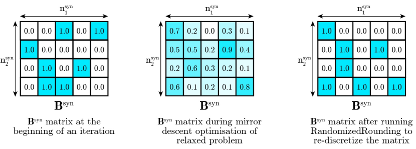
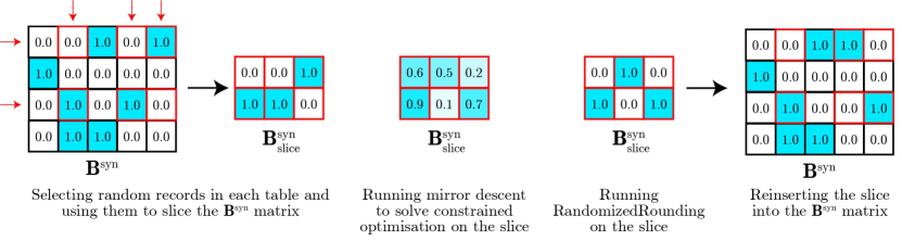
Figure 1: Top: diagram illustrating the original algorithm (Algorithm 1). Bottom: diagram illustrating the new algorithm (Algorithm 9).

To implement this algorithm, we begin by storing the bi-adjacency matrix as a sparse matrix $\bm{B}^{\text{syn}}\in\{0,1\}^{n_{1}^{\text{syn}}\times n_{2}^{\text{syn}}}$. We also introduce a new parameter $\alpha<1$, indicating which fraction of relations are learned in each iteration. Next, we define the slicing operation, which will be used to extract elements of $\bm{B}^{\text{syn}}$ before running the mirror-descent algorithm.

Definition 4.

Given a matrix $\bm{M}\in\mathbb{R}^{n_{1}\times n_{2}}$ and vectors $\bm{v}_{1}\in\{0,1\}^{n_{1}}$, $\bm{v}_{2}\in\{0,1\}^{n_{2}}$, we denote the slicing operation by $\bm{M}\left[\bm{v}^{1},\bm{v}^{2}\right]$. This operation yields a matrix with $\operatorname{sum}({\bm{v}^{\text{slice}}_{1}})$ rows and $\operatorname{sum}({\bm{v}^{\text{slice}}_{2}})$ columns. The $(i,j)$ entry of this matrix corresponds to the $(v^{1}_{i},v^{2}_{j})$ entry of $\bm{M}$, where $v^{1}_{i}$ is defined as the $i$-th nonzero entry of $\bm{v}^{1}$ (similarly for $v^{2}_{i}$).

The time and space complexity of the algorithm are reduced from $O(Tn_{1}^{\text{syn}}n_{2}^{\text{syn}})$ to $O(T\alpha^{2}n_{1}^{\text{syn}}n_{2}^{\text{syn}})$ by this strategy. Hence, by choosing smaller $\alpha$, we can reduce the time complexity of the algorithm.

Algorithm 9 Extension of Algorithm 1 to improve scalability.

Input: private relational database $\mathcal{B}=(\mathcal{D}_{1},\mathcal{D}_{2},\bm{B})$; privacy budget $(\varepsilon_{\text{rel}},\delta_{\text{rel}})$; individual synthetic tables $\mathcal{D}_{1}^{\text{syn}}$, $\mathcal{D}_{2}^{\text{syn}}$; workloads per iteration $K$; number of iterations $T$; number of relationship in synthetic tables: $m^{\text{syn}}$; slicing fraction $\alpha$

Initialize: $\bm{Q}=\emptyset,\hat{\bm{a}}=\emptyset$, $n_{1}^{\text{syn}}$ by $n_{2}^{\text{syn}}$ sparse matrix $\bm{B}^{\text{syn}}$ with entries $\in\{0,1\}$

for $t=1,\cdots,T$ do

     Select $K$ workloads via the exponential mechanism

     Append all queries associated with the newly selected workloads into $\bm{Q}$

     Add noise to the answers of the new queries and append them into $\hat{\bm{a}}$

     Randomly choose $\bm{v}^{\text{slice}}_{1}\in\{0,1\}^{n_{1}^{\text{syn}}}$, $\bm{v}^{\text{slice}}_{2}\in\{0,1\}^{n_{2}^{\text{syn}}}$ s.t. $\operatorname{sum}({\bm{v}^{\text{slice}}_{i}})=\operatorname{round}(\alpha n_{i}^{\text{syn}})$ for $i\in\{1,2\}$

     Set dense matrices $\bm{B}^{\text{syn}}_{\text{slice}}=\bm{B}^{\text{syn}}[\bm{v}^{\text{slice}}_{1},\bm{v}^{\text{slice}}_{2}]$ and $\bm{Q}_{\text{slice}}=\bm{Q}[\bm{v}^{\text{slice}}_{1},\bm{v}^{\text{slice}}_{2}]$

     Compute $m_{\text{slice}}=\operatorname{sum}(\bm{B}^{\text{syn}}_{\text{slice}})$

     Solve $\bm{B}^{\text{syn}}_{\text{slice}}={\arg\min}_{\begin{subarray}{c}B_{i,j}\in[0,1]\\ \operatorname{sum}(\bm{B}_{\text{slice}}^{\text{syn}})=m_{\text{slice}}\end{subarray}}\lVert\bm{Q}_{\text{slice}}\operatorname{flatten}(\bm{B}_{\text{slice}}^{\text{syn}})-\hat{\bm{a}}\rVert_{2}^{2}$ using mirror descent

     $\bm{B}^{\text{syn}}_{\text{slice}}=\operatorname{RandomizedRounding}(\bm{B}^{\text{syn}}_{\text{slice}})$

     Re-insert $\bm{B}^{\text{syn}}_{\text{slice}}$ into $\bm{B}^{\text{syn}}$: $\bm{B}^{\text{syn}}[\bm{v}^{\text{slice}}_{1},\bm{v}^{\text{slice}}_{2}]=\bm{B}^{\text{syn}}_{\text{slice}}$

end for

Output: $\mathcal{B}^{\text{syn}}=(\mathcal{D}^{\text{syn}}_{1},\mathcal{D}^{\text{syn}}_{2},\bm{B}^{\text{syn}})$

References

- Aydore et al. [2021] Sergul Aydore, William Brown, Michael Kearns, Krishnaram Kenthapadi, Luca Melis, Aaron Roth, and Ankit A Siva. Differentially private query release through adaptive projection. In International Conference on Machine Learning, pages 457–467. PMLR, 2021.
- Beaulieu-Jones et al. [2019] Brett K Beaulieu-Jones, Zhiwei Steven Wu, Chris Williams, Ran Lee, Sanjeev P Bhavnani, James Brian Byrd, and Casey S Greene. Privacy-preserving generative deep neural networks support clinical data sharing. Circulation: Cardiovascular Quality and Outcomes, 12(7):e005122, 2019.
- Bie et al. [2023] Alex Bie, Gautam Kamath, and Guojun Zhang. Private GANs, revisited. Transactions on Machine Learning Research, 2023.
- Blocki et al. [2012] Jeremiah Blocki, Avrim Blum, Anupam Datta, and Or Sheffet. The Johnson-Lindenstrauss transform itself preserves differential privacy. In 2012 IEEE 53rd Annual Symposium on Foundations of Computer Science, pages 410–419. IEEE, 2012.
- Blum et al. [2013] Avrim Blum, Katrina Ligett, and Aaron Roth. A learning theory approach to noninteractive database privacy. Journal of the ACM (JACM), 60(2):1–25, 2013.
- Boedihardjo et al. [2022] March Boedihardjo, Thomas Strohmer, and Roman Vershynin. Privacy of synthetic data: A statistical framework. IEEE Transactions on Information Theory, 69(1):520–527, 2022.
- Branch et al. [1999] Mary Ann Branch, Thomas F. Coleman, and Yuying Li. A subspace, interior, and conjugate gradient method for large-scale bound-constrained minimization problems. SIAM Journal on Scientific Computing, 21(1):1–23, 1999. doi: 10.1137/S1064827595289108. URL https://doi.org/10.1137/S1064827595289108.
- Bubeck et al. [2015] Sébastien Bubeck et al. Convex optimization: Algorithms and complexity. Foundations and Trends® in Machine Learning, 8(3-4):231–357, 2015.
- Bun and Steinke [2016] Mark Bun and Thomas Steinke. Concentrated differential privacy: Simplifications, extensions, and lower bounds. In Theory of Cryptography: 14th International Conference, TCC 2016-B, Beijing, China, October 31-November 3, 2016, Proceedings, Part I, pages 635–658. Springer, 2016.
- Cai et al. [2023] Kuntai Cai, Xiaokui Xiao, and Graham Cormode. Privlava: synthesizing relational data with foreign keys under differential privacy. Proceedings of the ACM on Management of Data, 1(2):1–25, 2023.
- Chen et al. [2015] Rui Chen, Qian Xiao, Yu Zhang, and Jianliang Xu. Differentially private high-dimensional data publication via sampling-based inference. In ACM SIGKDD international conference on knowledge discovery and data mining, pages 129–138, 2015.
- Dwork and Roth [2014] Cynthia Dwork and Aaron Roth. The algorithmic foundations of differential privacy. Foundations and Trends® in Theoretical Computer Science, 9(3–4):211–407, 2014.
- Eliáš et al. [2020] Marek Eliáš, Michael Kapralov, Janardhan Kulkarni, and Yin Tat Lee. Differentially private release of synthetic graphs. In Proceedings of the Fourteenth Annual ACM-SIAM Symposium on Discrete Algorithms, pages 560–578. SIAM, 2020.
- Francis [2024] Paul Francis. A comparison of syndiffix multi-table versus single-table synthetic data. arXiv preprint arXiv:2403.08463, 2024.
- Gaboardi et al. [2014] Marco Gaboardi, Emilio Jesús Gallego Arias, Justin Hsu, Aaron Roth, and Zhiwei Steven Wu. Dual query: Practical private query release for high dimensional data. In International Conference on Machine Learning, pages 1170–1178. PMLR, 2014.
- Ge et al. [2020] Chang Ge, Shubhankar Mohapatra, Xi He, and Ihab F Ilyas. Kamino: Constraint-aware differentially private data synthesis. arXiv preprint arXiv:2012.15713, 2020.
- Gupta et al. [2012] Anupam Gupta, Aaron Roth, and Jonathan Ullman. Iterative constructions and private data release. In Theory of Cryptography: 9th Theory of Cryptography Conference, TCC 2012, Taormina, Sicily, Italy, March 19-21, 2012. Proceedings 9, pages 339–356. Springer, 2012.
- Hardt et al. [2012] Moritz Hardt, Katrina Ligett, and Frank McSherry. A simple and practical algorithm for differentially private data release. Advances in neural information processing systems, 25, 2012.
- Hay et al. [2009] Michael Hay, Chao Li, Gerome Miklau, and David Jensen. Accurate estimation of the degree distribution of private networks. In 2009 Ninth IEEE International Conference on Data Mining, pages 169–178. IEEE, 2009.
- He [2021] Xi He. Differential privacy for complex data: Answering queries across multiple data tables. https://www.nist.gov/blogs/cybersecurity-insights/differential-privacy-complex-data-answering-queries-across-multiple, 2021.
- Johnson et al. [2018] Noah Johnson, Joseph P Near, and Dawn Song. Towards practical differential privacy for sql queries. Proceedings of the VLDB Endowment, 11(5):526–539, 2018.
- Jordon et al. [2019] James Jordon, Jinsung Yoon, and Mihaela Van Der Schaar. PATE-GAN: Generating synthetic data with differential privacy guarantees. In International conference on learning representations, 2019.
- Kaggle [2017] Kaggle. Kaggle 2017 survey results. https://www.kaggle.com/code/amberthomas/kaggle-2017-survey-results, 2017.
- Kotsogiannis et al. [2019] Ios Kotsogiannis, Yuchao Tao, Xi He, Maryam Fanaeepour, Ashwin Machanavajjhala, Michael Hay, and Gerome Miklau. Privatesql: a differentially private sql query engine. Proceedings of the VLDB Endowment, 12(11):1371–1384, 2019.
- Liu et al. [2023a] Jingcheng Liu, Jalaj Upadhyay, and Zongrui Zou. Optimal bounds on private graph approximation. arXiv preprint arXiv:2309.17330, 2023a.
- Liu et al. [2021a] Terrance Liu, Giuseppe Vietri, Thomas Steinke, Jonathan Ullman, and Steven Wu. Leveraging public data for practical private query release. In International Conference on Machine Learning, pages 6968–6977. PMLR, 2021a.
- Liu et al. [2021b] Terrance Liu, Giuseppe Vietri, and Steven Z Wu. Iterative methods for private synthetic data: Unifying framework and new methods. Advances in Neural Information Processing Systems, 34:690–702, 2021b.
- Liu et al. [2023b] Terrance Liu, Jingwu Tang, Giuseppe Vietri, and Steven Wu. Generating private synthetic data with genetic algorithms. In International Conference on Machine Learning, pages 22009–22027. PMLR, 2023b.
- Mami et al. [2022] Ciro Antonio Mami, Andrea Coser, Eric Medvet, Alexander TP Boudewijn, Marco Volpe, Michael Whitworth, Borut Svara, Gabriele Sgroi, Daniele Panfilo, and Sebastiano Saccani. Generating realistic synthetic relational data through graph variational autoencoders. arXiv preprint arXiv:2211.16889, 2022.
- McKenna et al. [2019] Ryan McKenna, Daniel Sheldon, and Gerome Miklau. Graphical-model based estimation and inference for differential privacy. In International Conference on Machine Learning, pages 4435–4444. PMLR, 2019.
- McKenna et al. [2021] Ryan McKenna, Gerome Miklau, and Daniel Sheldon. Winning the NIST contest: A scalable and general approach to differentially private synthetic data. arXiv preprint arXiv:2108.04978, 2021.
- McKenna et al. [2022] Ryan McKenna, Brett Mullins, Daniel Sheldon, and Gerome Miklau. Aim: An adaptive and iterative mechanism for differentially private synthetic data. arXiv preprint arXiv:2201.12677, 2022.
- Neunhoeffer et al. [2020] Marcel Neunhoeffer, Zhiwei Steven Wu, and Cynthia Dwork. Private post-gan boosting. arXiv preprint arXiv:2007.11934, 2020.
- Patki et al. [2016] Neha Patki, Roy Wedge, and Kalyan Veeramachaneni. The synthetic data vault. In 2016 IEEE International Conference on Data Science and Advanced Analytics (DSAA), pages 399–410. IEEE, 2016.
- Ranking [2023] DB-Engines Ranking. DB-engines ranking - popularity ranking of database management systems. https://db-engines.com/en/ranking, 2023.
- Ridgeway et al. [2021] Diane Ridgeway, Mary F Theofanos, Terese W Manley, and Christine Task. Challenge design and lessons learned from the 2018 differential privacy challenges. NIST Technical Note 2151, 2021.
- Rosenblatt et al. [2020] Lucas Rosenblatt, Xiaoyan Liu, Samira Pouyanfar, Eduardo de Leon, Anuj Desai, and Joshua Allen. Differentially private synthetic data: Applied evaluations and enhancements. arXiv preprint arXiv:2011.05537, 2020.
- Sala et al. [2011] Alessandra Sala, Xiaohan Zhao, Christo Wilson, Haitao Zheng, and Ben Y Zhao. Sharing graphs using differentially private graph models. In Proceedings of the 2011 ACM SIGCOMM conference on Internet measurement conference, pages 81–98, 2011.
- Schleich et al. [2019] Maximilian Schleich, Dan Olteanu, Mahmoud Abo-Khamis, Hung Q Ngo, and XuanLong Nguyen. Learning models over relational data: A brief tutorial. In Scalable Uncertainty Management: 13th International Conference, SUM 2019, Compiègne, France, December 16–18, 2019, Proceedings 13, pages 423–432. Springer, 2019.
- Schneider [2013] Rolf Schneider. Convex Bodies: The Brunn–Minkowski Theory. Encyclopedia of Mathematics and its Applications. Cambridge University Press, 2 edition, 2013.
- SmartNoise [2023] SmartNoise. Smartnoise sdk: Tools for differential privacy on tabular data. https://github.com/opendp/smartnoise-sdk, 2023.
- Stark and Parker [1995] Philip B Stark and Robert L Parker. Bounded-variable least-squares: an algorithm and applications. Computational Statistics, 10:129–129, 1995.
- Steinke [2022] Thomas Steinke. Composition of differential privacy & privacy amplification by subsampling. arXiv preprint arXiv:2210.00597, 2022.
- Tantipongpipat et al. [2019] Uthaipon Tantipongpipat, Chris Waites, Digvijay Boob, Amaresh Ankit Siva, and Rachel Cummings. Differentially private mixed-type data generation for unsupervised learning. arXiv preprint arXiv:1912.03250, 1:13, 2019.
- Tao et al. [2021] Yuchao Tao, Ryan McKenna, Michael Hay, Ashwin Machanavajjhala, and Gerome Miklau. Benchmarking differentially private synthetic data generation algorithms. arXiv preprint arXiv:2112.09238, 2021.
- Thaler et al. [2012] Justin Thaler, Jonathan Ullman, and Salil Vadhan. Faster algorithms for privately releasing marginals. In International Colloquium on Automata, Languages, and Programming, pages 810–821. Springer, 2012.
- Ullman and Vadhan [2020] Jonathan Ullman and Salil Vadhan. PCPs and the hardness of generating synthetic data. Journal of Cryptology, 33(4):2078–2112, 2020.
- Upadhyay [2013] Jalaj Upadhyay. Random projections, graph sparsification, and differential privacy. In International Conference on the Theory and Application of Cryptology and Information Security, pages 276–295. Springer, 2013.
- Vietri et al. [2020] Giuseppe Vietri, Grace Tian, Mark Bun, Thomas Steinke, and Steven Wu. New oracle-efficient algorithms for private synthetic data release. In International Conference on Machine Learning, pages 9765–9774. PMLR, 2020.
- Vietri et al. [2022] Giuseppe Vietri, Cedric Archambeau, Sergul Aydore, William Brown, Michael Kearns, Aaron Roth, Ankit Siva, Shuai Tang, and Steven Z Wu. Private synthetic data for multitask learning and marginal queries. Advances in Neural Information Processing Systems, 35:18282–18295, 2022.
- Wang et al. [2023] Hao Wang, Shivchander Sudalairaj, John Henning, Kristjan Greenewald, and Akash Srivastava. Post-processing private synthetic data for improving utility on selected measures. In Conference on Neural Information Processing Systems, 2023.
- Xie et al. [2018] Liyang Xie, Kaixiang Lin, Shu Wang, Fei Wang, and Jiayu Zhou. Differentially private generative adversarial network. arXiv preprint arXiv:1802.06739, 2018.
- Xu et al. [2023] Kai Xu, Georgi Ganev, Emile Joubert, Rees Davison, Olivier Van Acker, and Luke Robinson. Synthetic data generation of many-to-many datasets via random graph generation. In International Conference on Learning Representations, 2023.
- Yang et al. [2022] Jingyi Yang, Peizhi Wu, Gao Cong, Tieying Zhang, and Xiao He. Sam: Database generation from query workloads with supervised autoregressive models. In Proceedings of the 2022 International Conference on Management of Data, pages 1542–1555, 2022.
- Zhang et al. [2017] Jun Zhang, Graham Cormode, Cecilia M Procopiuc, Divesh Srivastava, and Xiaokui Xiao. PrivBayes: Private data release via Bayesian networks. ACM Transactions on Database Systems (TODS), 42(4):1–41, 2017.
- Zhang et al. [2021] Sen Zhang, Weiwei Ni, and Nan Fu. Differentially private graph publishing with degree distribution preservation. Computers & Security, 106:102285, 2021.