Mitigating Object Hallucination via Data Augmented Contrastive Tuning

Abstract

Despite their remarkable progress, Multimodal Large Language Models (MLLMs) tend to hallucinate factually inaccurate information. In this work, we address object hallucinations in MLLMs, where information is offered about an object that is not present in the model input. We introduce a contrastive tuning method that can be applied to a pretrained off-the-shelf MLLM for mitigating hallucinations, while preserving its general vision-language capabilities. For a given factual token, we create a hallucinated token through generative data augmentation by selectively altering the ground-truth information. The proposed contrastive tuning is applied at the token level to improve the relative likelihood of the factual token compared to the hallucinated one. Our thorough evaluation confirms the effectiveness of contrastive tuning in mitigating hallucination. Moreover, the proposed contrastive tuning is simple, fast, and requires minimal training with no additional overhead at inference.

1 Introduction

Recent advancements in Large Language Models (LLMs) [1, 2, 3, 4, 5, 6, 7] have laid the foundation for the development of highly capable multimodal LLMs (MLLMs) [6, 8, 9, 10, 11, 12]. MLLMs can process additional modalities such as image or video, while retaining language understanding and generation capabilities. Despite their impressive performance across a variety of tasks, the issue of object hallucination in MLLMs presents a significant challenge to their widespread and reliable use [13, 14, 15, 16]. Object hallucination refers to generated language that includes descriptions of objects or their attributes that are not present in, or cannot be verified by, the given input. We illustrate a few examples of object hallucinations in Figure 1, where on the left LLaVA-v1.5${}_{\text{13B}}$ inaccurately describes a ‘toothpick’ in an image of utensils (knife, spoon, fork) as these items frequently appear together, while it missed identifying ‘Legos’ due to their rare occurrence with utensils. On the right, LLaVA-v1.5${}_{\text{13B}}$ incorrectly confirms the presence of a ‘tie’ for the image of a ‘wedding cake’. This is likely due to two reasons: first, the frequent co-occurrence of wedding attire such as ‘ties’ and ‘wedding cakes’, and second, MLLMs tend to answer ‘Yes’ for most instructions presented due to positive instruction bias in the training data [17, 16].

Prior work have attempted to address object hallucination in one of three key stages: inference [18, 19, 20, 21, 22, 23], pretraining [24, 25, 17], and finetuning [26, 27]. Inference-based methods aim to mitigate hallucinations during text generation, either through specialized decoding [20, 18, 28] or through iterative corrections [21, 29, 22], among others. One of the key limitations of such approaches is that they can substantially increase inference time and cost, and often require modifications to the serving infrastructure [21, 16]. Pretraining techniques, such as negative instruction tuning or contrastive learning, have also been used to mitigate object hallucination [17, 25]. The main limitation of such approaches is that they require massive training data (>500K samples) and can not be applied to off-the-shelf MLLMs. Finally, finetuning-based approaches attempt to mitigate object hallucination through preference optimization [26] or human feedback [24, 30], among others [31, 27]. Nonetheless, these methods may lead to decreased performance on general vision-language tasks as illustrated in Figure 2.

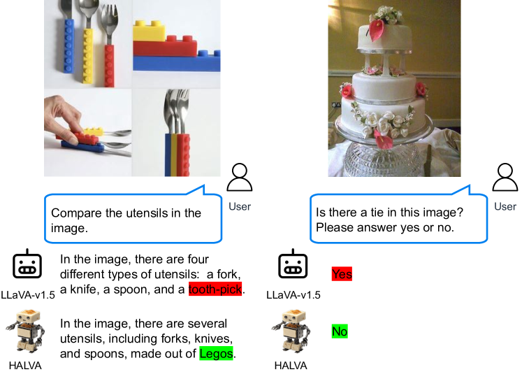
Figure 1: Examples of object hallucinations.

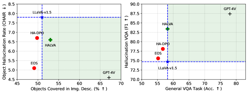
Figure 2: A high-level overview comparing the performance of HALVA with existing finetuning methods in mitigating object hallucination, and their ability on general vision-language tasks.

To achieve a method that can mitigate object hallucination in MLLMs without adding to inference time or requiring substantial re-training, all the while retaining out-of-the-box performance on general vision-language tasks, we propose data-augmented contrastive tuning. Our method consists of two key modules. It first applies generative data augmentation [32, 33] to obtain hallucinated responses based on the correct response and original image. Next, our novel contrastive objective is applied between a pair of correct and hallucinated tokens to reduce the relative log-probability of the hallucinated tokens in language generation. To ensure the MLLM retains its original performance in general vision-language tasks, we perform the contrastive tuning with a KL-divergence constraint [34, 35, 36] using a reference model, i.e., the MLLM is trained to minimize the contrastive loss while keeping the divergence at a minimal. We refer to MLLMs trained with this framework as Hallucination Attenuated Language and Vision Assistant (HALVA). We perform rigorous evaluations on hallucination benchmarks, showing the benefits of our method in mitigating hallucination in both generative and discriminative vision-language tasks. While the primary goal of this work is to mitigate object hallucinations, we take a further step to also evaluate on general vision-language hallucination benchmarks. The results show that our contrastive tuning method also provides benefits toward other forms of vision-language hallucinations. Finally, to ensure that the proposed contrastive tuning does not adversely affect the general language generation capabilities of MLLMs, we evaluate HALVA on popular vision-language benchmarks. Our extensive studies confirm the effectiveness of the proposed method in mitigating object hallucinations while retaining or improving the performance in general vision-language tasks.

Our main contribution is a contrastive framework to tune MLLMs for mitigating object hallucination in language generation. The proposed contrastive loss is applied between a pair of correct and hallucinated tokens, where the hallucinated responses are obtained through generative data augmentation. Our method is effective, fast, and can be directly adopted to off-the-shelf MLLMs. We open-source the code, HALVA checkpoints, and the complete output of the generative data augmentation module.

2 Method: Data augmented contrastive tuning

Consider an MLLM, denoted as $\pi_{\theta}$, which is trained in an auto-regressive manner to predict output $y$, for a given vision-language instruction $x\!=\!\{x_{v},x_{q}\}$. During inference, the generated sequence $s$ of length $N_{s}$ is represented as $\{z_{1},z_{2},\dots,z_{N_{s}}\}$, where $z$ represents the language tokens. $s$ contains hallucination if the occurrence of $z_{i}$ is not grounded in, or cannot be verified from, the input $x$. If the data used to train $\pi_{\theta}$ comprises frequent appearance of certain objects, the MLLM may generate responses based on the learned spurious correlations, while ignoring the given inputs [22, 16, 15, 37]. Here, we present our strategy to mitigate object hallucinations that may occur due to such co-occurrences. Our method consists of two main modules, generative data augmentation and contrastive tuning.

Generative data augmentation. Let’s assume $y^{+}$ and $y^{-}$ are a correct and hallucinated response, respectively, to a vision-language instruction $\{x_{v},x_{q}\}$. We design a simple data augmentation setup to generate $y^{-}$ by selectively altering the ground-truth objects and object-related attributes in $y^{+}$, thus introducing co-occurring concepts that are not present in $x_{v}$. Formally, we generate $y^{-}$ by replacing the object set $o$ of $y^{+}$, with hallucinated object set $o^{\prime}$, where $o^{\prime}\in{\mathbb{O}}\mid o^{\prime}\notin x_{v}$ and ${\mathbb{O}}$ is a set containing co-occurrences of objects. We define ${\mathbb{O}}\!=\!\{(o_{i},c_{i})\mid o_{i}\in U\text{ and }c_{i}\subseteq U\}$, where $o_{i}$ is an object, $c_{i}$ is a subset of objects that co-occur with $o_{i}$, and $U$ represents the universal set of all possible objects. An example is presented in Figure 3.

We approximate ${\mathbb{O}}$ for co-occurrences that are both closed set (${\mathbb{O}}_{cc}$) and open-set (${\mathbb{O}}_{oc}$). We prepare ${\mathbb{O}}_{cc}$ based on the co-occurrences of objects in a large object-centric dataset. For ${\mathbb{O}}_{oc}$ we sample object co-occurrences by directly prompting an LLM. In addition to generating descriptive responses, we also use a small set of Yes-or-No questions based on an existing visual question answering dataset, for which we generate $y^{-}$ by simply inverting $y^{+}$. This yields the contrastive response pairs $\{y^{+},y^{-}\}$, which we subsequently use in contrastive tuning. Additional details of generative data augmentation are presented in Appendix C.3.

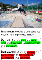
Figure 3: An example of contrastive pairs constructed through our generative data augmentation.

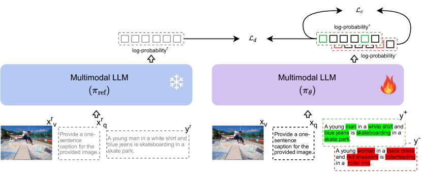
Figure 4: Overview of our method: Given a pair of vision-language instructions $\{x_{v},x_{q}\}$ and corresponding correct response $y^{+}$, we perform generative data augmentation to construct a hallucinated response $y^{-}$, by selectively altering the ground-truth objects. The proposed contrastive tuning is applied at a token-level to improve the relative probability of correct tokens in language generation.

Contrastive tuning. Given an off-the-shelf trained MLLM susceptible to hallucinations, our objective is to minimize the likelihood of generating hallucinated tokens using the contrastive pairs $\{y^{+},y^{-}\}$ obtained through generative data augmentation. To this end, we define a contrastive tuning objective based on the relative probabilities of correct and hallucinated tokens.

Let’s consider a simplified setup where $y^{+}$ has one ground-truth object and $y^{-}$ has a corresponding hallucinated object at the same index $i$. Furthermore, let us simplify by assuming that each word or object can be represented by a single token. Accordingly, our proposed contrastive objective can be formulated as:

$$\ell(x,y^{+},y^{-};\pi_{\theta})=-\log\frac{\pi_{\theta}(y_{i}^{+}|x)}{\pi_{\theta}(y_{i}^{+}|x)+\pi_{\theta}(y_{i}^{-}|x)},$$ (1)

where $x$ refers to the vision-language input pair $\{x_{v},x_{q}\}$. In practice, due to sub-word tokenization [38, 39], the correct and hallucinated words can be represented by different numbers of tokens. To accommodate this, we accumulate the log-probabilities of corresponding tokens at the word level, for both correct and hallucinated objects. For the sake of simplicity in our subsequent discussion, we will continue with the assumption that each word or object can be represented by a single token.

We define our final contrastive objective as:

$$\mathcal{L}_{c}=\frac{1}{N}\sum_{i=1}^{N}\ell(x_{i},y_{i}^{+},y_{i}^{-};\pi_{\theta}),$$ (2)

where $N$ refers to the total number of hallucinated tokens per sample.

As shown in Equation 1, our contrastive objective is directly applied at a token level. We only consider the likelihood of hallucinated tokens and their corresponding correct ones in the loss calculation, and the rest are discarded.

Let’s consider three situations regarding the behavior of $\mathcal{L}_{c}$ at a token level:

1. $\mathcal{L}_{c}\to 0$ when the $\pi_{\theta}(y_{i}^{-}|x)\ll\pi_{\theta}(y_{i}^{+}|x)$, i.e., the probability of hallucinated tokens are extremely small.

2. $\mathcal{L}_{c}\approx\log(2)$ when $\pi_{\theta}(y_{i}^{-}|x)\approx\pi_{\theta}(y_{i}^{+}|x)$, i.e., both the hallucinated and correct tokens are equally probable.

3. $\mathcal{L}_{c}>\log(2)$ when $\pi_{\theta}(y_{i}^{-}|x)>\pi_{\theta}(y_{i}^{+}|x)$, i.e., hallucinated tokens are more probable than the correct tokens.

Now, simply optimizing $\pi_{\theta}$ to achieve $\mathcal{L}_{c}\to 0$ may result in $\pi_{\theta}$ substantially diverging from its initial state, which may hurt its ability in general vision-language tasks. To mitigate this effect, we train $\pi_{\theta}$ with a KL-divergence constraint using a frozen reference model $\pi_{\text{ref}}$. For a given reference sample $\{x^{r},y^{r}\}$, the token-wise KL-divergence regularization term $\mathcal{L}_{d}$ is defined as:

$$\mathcal{L}_{d}=\sum^{T}_{t=1}{\pi_{\text{ref}}(y^{r}_{t}|x^{r})}\cdot\biggl{(}\log\Bigl{(}\pi_{\text{ref}}(y^{r}_{t}|x^{r})\Bigr{)}-\log\Bigl{(}\pi_{\theta}(y^{r}_{t}|x^{r})\Bigr{)}\biggr{)},$$ (3)

where $T$ is the total number of tokens in the reference sample. Note that $\{x^{r},y^{r}\}$ refer to standard vision-language instructions and their correct responses as hallucinated responses are not used to calculate divergence. By default, $\pi_{\text{ref}}$ and $\pi_{\theta}$ are initialized from the same checkpoint.

Finally, we train $\pi_{\theta}$ based on the final objective defined as:

$$\mathcal{L}=\mathcal{L}_{c}+\alpha\cdot\mathcal{L}_{d},$$ (4)

where $\alpha$ is a coefficient to control the divergence of $\pi_{\theta}$ during contrastive tuning. We present the pseudo code in Appendix A. The value of $\alpha$ is set based on in-depth ablation studies presented in Appendix B.

3 Experiment setup

Training data. We prepare vision-language instructions based on Visual Genome (VG) [40], which is an object-centric image dataset consisting of a total of 108K images and their annotations. Accordingly, we prepare the correct responses with both descriptive (e.g., Describe this image in detail.) and non-descriptive (e.g., <Question>, Please answer in one word, yes or no) instructions. Descriptive instructions include one-sentence captions, short descriptions, and detailed descriptions of images. Moreover, the non-descriptive question-answers are directly taken from [26]. We prepare the correct responses using Gemini Vision Pro [6] and based on the original images and ground-truth annotations. Subsequently, we perform generative data augmentation to obtain hallucinated responses, as described in Section 2. Our final training set consists of a total of $21.5$K vision-language instructions and their corresponding correct and hallucinated responses, which are then used in contrastive tuning.

Implementation details. We use LLaVA-v1.5 [9] as our base model considering its superior performance in general vision-language tasks and the availability of its code and models. LLaVA-v1.5 uses Vicuna-v1.5 [41, 5] as the language encoder and CLIP ViT-L${}_{\text{14}}$ [42] as the vision encoder. During training, we freeze the vision encoder and projection layers, and only train the LLM using LoRA [43]. We refer to the resulting contrastively tuned checkpoints as HALVA. All experiments are conducted on four A100-80GB GPUs. We utilize an effective batch size of 64 and train for $1$ epoch, using Cosine learning rate scheduler with a base learning rate of 5e${}^{\text{-6}}$. We experiment with both 7B and 13B variants of LLaVA-v1.5. The training time ranges from $1.5$ to $3$ hours for 7B and 13B variants, respectively. The additional implementation details are presented in Appendix C.

Evaluation setup. First, we evaluate HALVA on four object hallucination benchmarks encompassing both generative and discriminative tasks, including CHAIR [15], MME-Hall [44], AMBER [45], and MMHal-Bench [24]. Additionally, we perform a curiosity driven experiment to critically test the impact of our proposed contrastive tuning beyond object hallucination, using HallusionBench [46]. Furthermore, to ensure that our proposed contrastive tuning does not adversely affect the general language generation capabilities of MLLMs, we evaluate HALVA on four popular vision-language benchmarks: VQA-v2 [47], MM-Vet [48], TextVQA [49], and MME [44]. All evaluations are conducted three times, and we report average scores. In the case of GPT-4-based evaluation [24, 46], the performance slightly varies due to the randomness of GPT-4 generations. Therefore we also report the standard deviations.

4 Results

Earlier in Figure 2, we present a high-level overview of HALVA vs. existing finetuning approaches (e.g., HA-DPO [26] and EOS [27]) in mitigating object hallucinations and their effect on the general vision-language capabilities. Note that both HA-DPO [26] and EOS [27] are based on the same LLaVA-v1.5 model as HALVA, ensuring a fair comparison. We consider LLaVA-v1.5 as the lower bound and GPT-4V as strong reference point given its performance on the standard benchmarks.

Image description task. In Figure 2 left, we compare MLLMs on image description tasks assessing both hallucination rate (AMBER CHAIR) and their detailedness of generated image descriptions, captured through the number of ground-truth objects covered (AMBER Cover). Our goal is to mitigate hallucinations while retaining or improving the richness of image descriptions compared to LLaVA-v1.5. As shown, HALVA captures more ground-truth objects while hallucinating less than HA-DPO. Moreover, while EOS achieves a slightly lower hallucination rate, it degrades the detailedness of image descriptions, performing worse than the base model. This is an undesired artifact in MLLMs, particularly for tasks that require detailedness such as medical imaging analysis [13, 14].

Figure 5: Unlike HALVA, the existing finetuning approaches (HA-DPO, EOS) substantially diverge from the base model (LLaVA-v1.5), resulting in performance degradation in general tasks.

Question answering task. In Figure 2 right, we compare the performance of MLLMs on visual-question answering tasks using both object hallucination (AMBER F1) and general vision-language (TextVQA Acc.) benchmarks. As shown, both HA-DPO and EOS underperform HALVA in mitigating object hallucination and even deteriorate general vision-language abilities compared to the base model. These results show the shortcomings of existing approaches, which we address in this work.

To further understand the limitations of existing methods in greater detail, we measure divergence from the base model in Figure 5. Here we observe that unlike HALVA, both HA-DPO and EOS substantially diverge from the base model, resulting in poor performance in general vision-language tasks.

4.1 Evaluation on object hallucination

CHAIR. MLLMs can be prone to hallucinations when generating detailed image descriptions [16, 15, 45]. To assess the impact of our proposed contrastive tuning in such scenarios, we evaluate HALVA on CHAIR, which stands for Caption Hallucination Assessment with Image Relevance [15]. This metric calculates the number of objects that appear in the image caption but are not present in the image. Specifically, CHAIR measures hallucination at two levels: instance-level and sentence-level. During this task, HALVA is prompted with ‘Describe this image in detail’, allowing for the generation of detailed image descriptions. The results in Table 1 demonstrate that HALVA substantially reduces hallucination in image descriptions compared to the base variants. For instance, compared to LLaVA-v1.5${}_{\text{7B}}$, HALVA${}_{\text{7B}}$ reduces sentence-level hallucination from $50.0$ to $41.4$. Furthermore, HALVA${}_{\text{7B}}$ outperforms or matches the performance of other hallucination mitigation methods, such as OPERA [50], EOS [27], and HA-DPO [26]. It should be noted that our proposed contrastive tuning does not negatively impact the language generation ability or expressiveness of MLLMs, unlike EOS [27], which substantially reduces the average generation length from $100$ to $85$ and $79$ for the 13B and 7B variants, respectively. As discussed earlier in Section 4, such a degree of reduction can lead to missing key details in image descriptions and are undesirable for MLLMs. In contrast, HALVA maintains the same generation length as the base model, e.g., $98$ vs. $100$, while effectively reducing hallucination. However, a limitation of CHAIR [15] is that it does not consider other key aspects of language generation, such as coverage of objects and detailedness of descriptions, when evaluating hallucination. Therefore, we also evaluate on AMBER [45], a more recent object hallucination benchmark, which we discuss later.

Table 1: Results on CHAIR. ^‡ and ^† indicate that the reported values are from [51] and [27]. ^*Results are computed by us, using their official checkpoints. C_i and C_s refer to CHAIR at instance and sentence levels.

Method	C${}_{i}(\downarrow)$	C${}_{s}(\downarrow)$	Len.
mPLUG-Owl‡7B [52]	30.2	76.8	98.5
MultiModal-GPT$\textsuperscript{\textdaggerdbl}_{\text{7B}}$ [53]	18.2	36.2	45.7
MiniGPT-v2$\textsuperscript{\textdaggerdbl}_{\text{7B}}$ [51]	8.7	25.3	56.5
InstructBlip${}_{\text{7B}}$ [10]	17.5	62.9	102.9
LLaVA-v1.5$\textsuperscript{\textdagger}_{\text{7B}}$ [9]	15.4	50.0	100.6
LLaVA-v1.5${}_{\text{7B}}$ w/ EOS [27]	12.3	40.2	79.7
LLaVA-v1.5${}_{\text{7B}}$ w/ OPERA [50]	12.8	44.6	-
LLaVA-v1.5$\textsuperscript{*}_{\text{7B}}$ w/ HA-DPO [26]	11.0	38.2	91.0
HALVA${}_{\text{7B}}$ (Ours)	11.7↓3.7	41.4↓8.6	92.2
MiniGPT-4†13B [54]	9.2	31.5	116.2
InstructBlip${}_{\text{13B}}$ [10]	16.0	51.2	95.6
LLaVA$\textsuperscript{\textdaggerdbl}_{\text{13B}}$ [8]	18.8	62.7	90.7
LLaVA-v1.5$\textsuperscript{\textdagger}_{\text{13B}}$ [9]	13.0	47.2	100.9
LLaVA-v1.5${}_{\text{13B}}$ w/ EOS [27]	11.4	36.8	85.1
HALVA${}_{\text{13B}}$ (Ours)	12.8↓0.2	45.4↓1.8	98.0

Table 2: Results on MME-Hall. ^‡ indicates that the reported values are from [16]. ^*Results are computed by us, using their official checkpoints.

Method	MME-Hall $(\uparrow)$
Cheetor${}_{\text{7B}}\textsuperscript{\textdaggerdbl}$ [55]	473.4
LRV-Instruction${}_{\text{7B}}\textsuperscript{\textdaggerdbl}$ [17]	528.4
Otter${}_{\text{7B}}\textsuperscript{\textdaggerdbl}$ [56]	483.3
mPLUG-Owl2${}_{\text{7B}}\textsuperscript{\textdaggerdbl}$ [57]	578.3
Lynx${}_{\text{7B}}\textsuperscript{\textdaggerdbl}$ [58]	606.7
Qwen-VL-Chat${}_{\text{7B}}\textsuperscript{\textdaggerdbl}$ [59]	606.6
LLaMA-Adapter V2${}_{\text{7B}}\textsuperscript{\textdaggerdbl}$ [60]	493.3
LLaVA-v1.5${}_{\text{7B}}$ [9]	648.3
LLaVA-v1.5$\textsuperscript{*}_{\text{7B}}$ w/ HA-DPO [26]	618.3
LLaVA-v1.5$\textsuperscript{*}_{\text{7B}}$ w/ EOS [27]	606.7
LLaVA-v1.5${}_{\text{7B}}$ w/ VCD [20]	604.7
HALVA${}_{\text{7B}}$ (Ours)	665.0↑16.7
BLIVA${}_{\text{11B}}\textsuperscript{\textdaggerdbl}$ [61]	580.0
MMICL${}_{\text{12B}}\textsuperscript{\textdaggerdbl}$ [62]	568.4
InstructBLIP${}_{\text{13B}}\textsuperscript{\textdaggerdbl}$ [10]	548.3
SPHINX${}_{\text{13B}}\textsuperscript{\textdaggerdbl}$ [63]	668.3
Muffin${}_{\text{13B}}\textsuperscript{\textdaggerdbl}$ [64]	590.0
LLaVA-v1.5${}_{\text{13B}}$ [9]	643.3
HALVA${}_{\text{13B}}$ (Ours)	675.0↑31.7

MME-Hall. We evaluate HALVA on discriminative tasks using MME [44]. Specifically, we utilize the hallucination subset of MME, which consists of four object-related subtasks: existence, count, position, and color, referred to as MME-Hall. The full score of each category is $200$, making the maximum total score $800$. The results presented in Table 2 demonstrate that HALVA substantially improves performance compared to the base model LLaVA-v1.5. For instance, HALVA${}_{\text{13B}}$ achieves a score of $675.0$, resulting in a performance gain of $31.7$ points with respect to the base model LLaVA-v1.5${}_{\text{13B}}$. Moreover, as presented in Table 2, existing methods (HA-DPO, EOS, VCD) are ineffective in mitigating hallucinations across such broad categories and worsen the performance compared to their base model. The detailed results of MME-Hall are presented in Appendix B.

Table 3: Results on AMBER. Cover.: coverage of ground-truth objects; Hall.: Hallucination Rate; Cog.: Cognition; F1${}_{\text{E}}$, F1${}_{\text{A}}$, and F1${}_{\text{R}}$ refer to F1 scores of Existence, Attribute, and Relation subsets. The final F1 is calculated across all sub-tasks. ^‡ indicates that the reported values are from [45]. ^*Results are computed by us, using their official checkpoint.

Method	Generative Task				Discriminative Task
	CHAIR ${(\downarrow)}$	Cover. ${(\uparrow)}$	Hall. ${(\downarrow)}$	Cog. ${(\downarrow)}$	F1${}_{\text{E}}$	F1${}_{\text{A}}$	F1${}_{\text{R}}$	F1
mPLUG-Owl$\textsuperscript{\textdaggerdbl}_{\text{7B}}$ [52]	21.6	50.1	76.1	11.5	17.2	22.9	6.2	18.9
LLaVA$\textsuperscript{\textdaggerdbl}_{\text{7B}}$ [8]	11.5	51.0	48.8	5.5	8.4	48.6	58.1	32.7
MiniGPT-4$\textsuperscript{\textdaggerdbl}_{\text{7B}}$ [54]	13.6	63.0	65.3	11.3	80.0	43.7	52.7	64.7
mPLUG-Owl2$\textsuperscript{\textdaggerdbl}_{\text{7B}}$ [57]	10.6	52.0	39.9	4.5	89.1	72.4	54.3	78.5
InstructBLIP$\textsuperscript{\textdaggerdbl}_{\text{7B}}$	8.8	52.2	38.2	4.4	89.0	76.3	67.6	81.7
LLaVA-v1.5$\textsuperscript{\textdaggerdbl}_{\text{7B}}$	7.8	51.0	36.4	4.2	64.6	65.6	62.4	74.7
LLaVA-v1.5$\textsuperscript{*}_{\text{7B}}$ w/ HA-DPO [26]	6.7	49.8	30.9	3.3	88.1	66.1	68.8	78.1
LLaVA-v1.5$\textsuperscript{*}_{\text{7B}}$ w/ EOS [27]	5.1	49.1	22.7	2.0	82.8	67.4	69.2	75.6
HALVA${}_{\text{7B}}$ (Ours)	6.6↓1.2	53.0↑2.0	32.2↓4.2	3.4↓0.8	93.3↑28.7	77.1↑11.5	63.1↑0.7	83.4↑8.7
LLaVA-v1.5${}_{\text{13B}}$	6.6	51.9	30.5	3.3	78.5	70.2	45.0	73.1
HALVA${}_{\text{13B}}$ (Ours)	6.4↓0.2	52.6↑0.7	30.4↓0.1	3.2↓0.1	92.6↑14.1	81.4↑11.2	73.5↑28.5	86.5↑13.4
GPT-4V‡ [12]	4.6	67.1	30.7	2.6	94.5	82.2	83.2	87.4

AMBER. To evaluate performance on both generative and discriminative tasks, we use AMBER [45], which measures hallucination using several metrics. For generative tasks, AMBER assesses the frequency of hallucinated objects in image descriptions, similar to [15]. Moreover, AMBER evaluates hallucination in three additional aspects of generative abilities: the number of ground-truth objects covered in the description, the hallucination rate, and the similarity of hallucinations in MLLMs to those observed in human cognition. Discriminative tasks are categorized into three broad groups: existence, attribute, and relation, each assessed using F1 scores. For additional details on these evaluation metrics, we refer the reader to [45].

The results presented in Table 3 demonstrate that HALVA outperforms the base model LLaVA-v1.5 by a large margin, in both generative and discriminative tasks. For instance, HALVA${}_{\text{7B}}$ reduces hallucination in caption generation from $7.8$ to $6.6$, while increasing the coverage of ground-truth objects in the descriptions from $51\%$ to $53\%$. This confirms that our method reduces hallucination without compromising the descriptive power of MLLMs. On the other hand, while HA-DPO and EOS report slightly lower hallucination rates, the number of ground-truth objects covered is reduced to $49.8\%$ and $49.1\%$, respectively. This indicates a degradation in the overall performance of these MLLMs on general tasks. Moreover, our contrastive tuning method substantially enhances performance on discriminative tasks, for both 7B and 13B variants. For instance, HALVA${}_{\text{7B}}$ improves the F1-score on the existence category from $64.6\%$ to $93.3\%$. Additionally, HALVA${}_{\text{13B}}$ improves the F1 score on relation-based tasks from $45.0\%$ to $73.5\%$. Overall, HALVA${}_{\text{7B}}$ outperforms both HA-DPO and EOS on discriminative tasks by a large margin, achieving a $5.3$ and $7.8$ point higher F1 score respectively. Furthermore, HALVA${}_{\text{13B}}$ achieves a comparable performance to GPT-4V on discriminative tasks, with $86.5\%$ vs. $87.4\%$.

Table 4: Results on MMHal-Bench. ^† and ^‡ indicate that the reported values are from [24] and [25]. ^*Results are computed by us, using their official checkpoint.

Method	Overall Score $(\uparrow)$	Hall. Rate $(\downarrow)$
Kosmos-2‡ [65]	1.69	0.68
IDEFIC$\textsuperscript{\textdaggerdbl}_{\textsc{9B}}$ [66]	1.89	0.64
InstructBLIP$\textsuperscript{\textdaggerdbl}_{\textsc{7B}}$ [10]	2.10	0.58
LLaVA$\textsuperscript{\textdaggerdbl}_{\textsc{7B}}$ [8]	1.55	0.76
LLaVA-SFT${}_{\textsc{7B}}$ [24]	1.76	0.67
LLaVA-RLHF${}_{\textsc{7B}}$ [24]	2.05	0.68
LLaVA-v1.5${}_{\textsc{7B}}$ [9]	2.11±0.05	0.54±0.01
LLaVA-v1.5${}_{\textsc{7B}}$ w/ HACL [25]	2.13	0.50
LLaVA-v1.5$\textsuperscript{*}_{\textsc{7B}}$ w/ HA-DPO [26]	1.97	0.60
LLaVA-v1.5$\textsuperscript{*}_{\textsc{7B}}$ w/ EOS [27]	2.03	0.59
HALVA${}_{\text{7B}}$ (Ours)	2.25${}_{{\color[rgb]{0.0,0.5,0.0}{\mathbf{\uparrow 0.14}}}}^{\pm 0.09}$	0.54${}_{{\color[rgb]{0.0,0.5,0.0}{\mathbf{\downarrow 0.00}}}}^{\pm 0.01}$
LLaVA$\textsuperscript{\textdagger}_{\textsc{13B}}$ [8]	1.11	0.84
InstructBLIP$\textsuperscript{\textdaggerdbl}_{\textsc{13B}}$ [10]	2.14	0.58
LLaVA-SFT${}_{\textsc{13B}}$ [24]	2.43	0.55
LLaVA-RLHF${}_{\textsc{13B}}$ [24]	2.53	0.57
LLaVA-v1.5${}_{\textsc{13B}}$ [9]	2.37±0.02	0.50±0.00
HALVA${}_{\text{13B}}$ (Ours)	2.58${}_{{\color[rgb]{0.0,0.5,0.0}{\mathbf{\uparrow 0.21}}}}^{\pm 0.07}$	0.45${}_{{\color[rgb]{0.0,0.5,0.0}{\mathbf{\downarrow 0.05}}}}^{\pm 0.02}$

Table 5: Results on HallusionBench. ^† indicates that the reported values are from [46]. ^*Results are computed by us, using their official checkpoint.

Method	Hard Acc. ($\uparrow$)	Overall Acc. ($\uparrow$)
mPLUG_Owl-v1$\textsuperscript{\textdagger}_{\text{7.2B}}$ [52]	29.77	43.93
MiniGPT5$\textsuperscript{\textdagger}_{\text{7B}}$ [67]	28.37	40.30
MiniGPT4$\textsuperscript{\textdagger}_{\text{7B}}$ [54]	27.67	35.78
InstructBLIP$\textsuperscript{\textdagger}_{\text{7B}}$ [10]	45.12	45.26
BLIP2$\textsuperscript{\textdagger}_{\text{7B}}$ [11]	40.70	40.48
mPLUG_Owl-v2$\textsuperscript{\textdagger}_{\text{7B}}$ [57]	39.07	47.30
LRV_Instruction$\textsuperscript{\textdagger}_{\text{7B}}$ [17]	27.44	42.78
LLaVA-1.5$\textsuperscript{*}_{\text{7B}}$ [9]	41.47±0.13	47.09±0.14
HALVA${}_{\text{7B}}$ (Ours)	45.81${}_{{\color[rgb]{0.0,0.5,0.0}{\mathbf{\uparrow 4.34}}}}^{\pm 0.00}$	48.95${}_{{\color[rgb]{0.0,0.5,0.0}{\mathbf{\uparrow 1.86}}}}^{\pm 0.13}$
Qwen-VL$\textsuperscript{\textdagger}_{\text{9.6B}}$ [59]	24.88	39.15
Open-Flamingo$\textsuperscript{\textdagger}_{\text{9B}}$ [68]	27.21	38.44
BLIP2-T5$\textsuperscript{\textdagger}_{\text{12B}}$ [11]	43.49	48.09
LLaVA-1.5$\textsuperscript{\textdagger}_{\text{13B}}$ [9]	29.77	46.94
LLaVA-1.5$\textsuperscript{*}_{\text{13B}}$ [9]	35.97±0.13	46.50±0.09
HALVA${}_{\text{13B}}$ (Ours)	42.87${}_{{\color[rgb]{0.0,0.5,0.0}{\mathbf{\uparrow 6.90}}}}^{\pm 0.13}$	49.10${}_{{\color[rgb]{0.0,0.5,0.0}{\mathbf{\uparrow 2.16}}}}^{\pm 0.05}$
GPT4V† [12]	37.67	65.28
Gemini Pro Vision† [6]	30.23	36.85

MMHal-Bench. We also conduct LLM-assisted hallucination evaluation to rigorously test for potential hallucinations in generated responses that might not be captured when validated against a limited ground-truth information, as done in [15]. We utilize MMHal-Bench [24], which evaluates hallucination across $12$ object-topics, including object attributes, presence of adversarial objects, and spatial relations, among others. Following [24], we use GPT-4 [12] as the judge to rate the responses on a scale of $0$ to $6$, with respect to standard human-generated answers and other ground-truth information of the images. The results presented in Table 4 demonstrate that HALVA considerably improves performance with respect to LLaVA-v1.5. Furthermore, we observe that our approach is more effective in mitigating hallucination than existing RLHF, SFT, or DPO-based methods. For example, HALVA${}_{\text{7B}}$ achieves a score of $2.25$ surpassing the 7B variants of RLHF, DPO, and SFT -based methods, which report scores of $2.05$, $1.97$, and $1.76$, respectively. Moreover, HALVA${}_{\text{13B}}$ reduces the hallucination rate to $0.45$, compared to $0.57$ for LLaVA-RLHF. Note that as LLaVA-RLHF and LLaVA-SFT use the same language and vision encoders as HALVA (Vicuna-V1.5 [41] and ViT-L/14 [42]), ensuring a fair direct comparison. The detailed results for the individual categories are presented in Appendix B.

4.2 Evaluation on hallucination benchmarks beyond object hallucination

To further stress-test our method on other forms of vision-language hallucinations that are not restricted to objects and may occur due to visual illusions, we evaluate performance on HallusionBench [46]. The results presented in Table 5 demonstrate that our proposed method directly benefits other forms of vision-language hallucinations as well. HALVA${}_{\text{7B}}$ and HALVA${}_{\text{13B}}$ improve overall accuracy by $1.86\%$ and $2.16\%$, respectively, compared to their base models. Moreover, we find that HALVA considerably improves performance ($4.34\%$-$6.90\%$) on the Hard Set of HallusionBench, which consists of human-edited image-question pairs specially crafted to elicit hallucinations in MLLMs. Detailed results on HallusionBench are presented in Appendix B.

Table 6: Results on general vision-language tasks. Our study confirms that our method not only mitigates hallucinations but also retains or improves performance on general vision-language tasks. ^∗Results are computed by us, using their official checkpoint. Both HA-DPO${}_{\text{7B}}$ and EOS${}_{\text{7B}}$ are also based on LLaVA-v1.5${}_{\text{7B}}$, similar to HALVA${}_{\text{7B}}$.

Method	VQA${}^{\text{v2}}_{\uparrow}$	MM-Vet↑	TextVQA↑	MME↑
LLaVA-v1.5${}_{\text{7B}}$	78.5	31.1	58.2	1510.7
HA-DPO${}_{\text{7B}}$	77.6${}_{{\color[rgb]{1,0,0}{\mathbf{\downarrow 0.9}}}}^{*}$	30.7${}_{{\color[rgb]{1,0,0}{\mathbf{\downarrow 0.4}}}}^{*}$	56.7${}_{{\color[rgb]{1,0,0}{\mathbf{\downarrow 1.5}}}}^{*}$	1502.6↓8.1
EOS${}_{\text{7B}}$	77.6${}_{{\color[rgb]{1,0,0}{\mathbf{\downarrow 0.9}}}}^{*}$	31.4${}_{{\color[rgb]{0.0,0.5,0.0}{\mathbf{\uparrow 0.3}}}}^{*}$	55.2${}_{{\color[rgb]{1,0,0}{\mathbf{\downarrow 3.0}}}}^{*}$	1424.4${}_{{\color[rgb]{1,0,0}{\mathbf{\downarrow 102.6}}}}^{*}$
HALVA${}_{\text{7B}}$ (Ours)	78.5${}_{\mathbf{{~{}0.0}}}$	32.1↑1.0	58.2${}_{\mathbf{{~{}0.0}}}$	1527.0↑16.3

4.3 Evaluation on non-hallucination benchmarks

We further assess HALVA on standard vision-language tasks using four popular benchmarks: VQA-v2 [47], MM-Vet [48], TextVQA [49], and MME [44]. The results presented in Table 6 show that HALVA maintains or improves performance with respect to the base LLaVA-v1.5. For example, HALVA${}_{\text{7B}}$ improves on MME and MM-Vet by $16.3$ and $1\%$ respectively, while retaining the same performance on TextVQA and VQA-v2. We note that unlike HALVA, existing object hallucination methods such as HA-DPO [26] and EOS [27] (also based on LLaVA-v1.5${}_{\text{7B}}$), exhibit deterioration in general tasks when tuned for hallucination mitigation.

Figure 6: Changes in the model state due to our contrastive tuning with varying $\alpha$. By default, we use $\alpha\!=0.4$ for HALVA${}_{\text{7B}}$.

4.4 Ablation study

Recalling our final objective function, which combines the contrastive loss ($\mathcal{L}_{c}$) and KL divergence ($\mathcal{L}_{d}$), defined as $\mathcal{L}=\mathcal{L}_{c}+\alpha\cdot\mathcal{L}_{d}$, we examine the change in model state with varying $\alpha$, as depicted in Figure 6. The $y$ axis represents the extent to which the model diverges from its initial state due to contrastive tuning, while the $x$ axis shows the change in the relative log-probability of the hallucinated tokens. Each data point in this figure represents the calculated contrastive loss and divergence after training for different values of $\alpha$. The figure illustrates that with a very low $\alpha$, e.g. $0.01$, the model substantially diverges from its initial state. As $\alpha$ increases, the model tends to retain a state similar to the base model. We empirically find that $\alpha\!=\!0.4$ works optimally for HALVA${}_{\text{7B}}$. In-depth ablation studies on the proposed loss, generative data augmentation, and divergence measure for $\mathcal{L}_{d}$ are presented in Appendix B.

4.5 Qualitative analysis

A qualitative comparison of HALVA to the base model LLaVA-v1.5 is shown in Figure 7, with additional examples in Appendix D. HALVA consistently provides more accurate image descriptions than LLaVA-v1.5. For example, in Figure 7 (A), LLaVA-v1.5 hallucinates ‘people’, ‘airport staff’, ‘passengers’ in an image of a parked airplane. In contrast, HALVA accurately describes the image with necessary details. Additionally, our method does not exhibit LLaVA-v1.5’s tendency to answer ‘Yes’ to most questions, which can contribute to hallucinations. This is shown in Figure 7 (B), where HALVA correctly answers ‘Yes’ when asked ‘Is the cloud white in the image?’ and responds with ‘No’ when asked ’Is the cloud black in this image?’, whereas LLaVA-v1.5 answers ‘Yes’ to both cases. Lastly, we present an example of hallucination caused by visual illusion in Figure 7 (C). While HALVA is not explicitly trained for such vision-language hallucinations, our approach shows some ability to mitigate it.

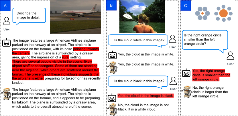
Figure 7: A sample qualitative demonstration of HALVA ()  and LLaVA-v1.5 (). Our proposed contrastive tuning effectively mitigates hallucination under different setups: (A) image description , (B) visual question answering , (C) visual illusion. Hallucinations are highlighted in red.

5 Related work

Multimodal LLMs. Vision-language models (VLMs) often align image and text features in a shared embedding space, as pioneered by CLIP [42] and ALIGN [69], followed by others [70, 71, 72, 73]. This alignment is achieved through contrastive learning on large image-text datasets. VLMs show strong generalization across various tasks. Leveraging LLMs and vision encoders from VLMs like CLIP, recent MLLMs [8, 54, 6, 12, 10, 11, 65, 61, 10, 59, 74] further enhance visual perception, understanding, and reasoning. While some MLLMs are open-source, others are only accessible through APIs [12, 6, 59]. Among publicly available MLLMs, LLaVA [8, 9] is widely used due to its simplicity and the availability of code, models, and training data. This makes it a suitable base model for demonstrating our method’s applicability to off-the-shelf MLLMs.

Hallucination in MLLMs. Multimodal hallucination generally refers to the misrepresentation of verifiable information in relation to the given input. This phenomenon has been primarily studied in the context of object hallucination [15, 16, 22, 24, 23]. Prior work to mitigate this issue can be categorized into three phases: pretraining, where techniques include using balanced instruction-tuning data with equal positive and negative examples [17] or generating and correcting image-instruction pairs on-the-fly [75]; inference, with methods involving specialized decoding strategies[20, 18, 28] or iterative corrections using offline models to detect and correct hallucinations at inference time [22, 19]; and finetuning, with approaches relying on human feedback [24, 30] to train reward models or employing preference optimization techniques [26]. While finetuning methods are a more efficient direction as they do not require training from scratch (unlike pretraining-based methods) nor changes in the serving infrastructure (unlike inference-based methods), existing finetuning approaches deteriorate the performance of the base model on general vision-language tasks (see Figures 2 and 5). To address this, we introduce generative data augmented contrastive tuning, which is effective in mitigating object hallucination on a broad set of vision-language tasks while retaining or improving the general vision-language ability of the base model.

6 Concluding remarks

To mitigate object hallucination in MLLMs, we performed generative data augmentation to construct hallucinated responses using a set of vision-language instructions. We then introduced a contrastive tuning method that can be applied to off-the-shelf MLLMs to mitigate hallucinations while preserving their capability in general vision-language tasks. Our proposed contrastive loss simply mitigates object hallucinations in MLLMs by lowering the relative probability of hallucinated tokens in generation. Our extensive study confirms the effectiveness of our method in mitigating object hallucinations and beyond, while retaining or even improving their performance on general vision-language tasks.

Broader impact & limitations. In this work, we focused on mitigating object hallucinations in MLLMs. However, MLLMs also suffer from other forms of hallucinations that may occur due to over-reliance on language while ignoring other input modalities, among others. While we showed some promising results on generalization to other forms, a rigorous exploration of these directions is left for future work. Additionally, the proposed generative data augmentation and contrastive tuning method may be generalized to other foundation models with accessible weights. Finally, we believe our method may have applications in other areas as well. For example, it might be adapted to mitigate bias and harmful language generation, among others. We leave this exploration for future research.

Appendix

The organization of the appendix is as follows:

• A: Pseudo Code

• B: Additional Experiments and Results

• C: Implementation Details

• D: Qualitative Results

Appendix A Pseudo Code

Our proposed contrastive tuning is fairly straightforward to implement. Below, we provide a PyTorch-based pseudo code. Please note that this is a minimal implementation to present the key steps of our algorithm. Some of the intermediary and rudimentary steps (e.g., ignoring padded inputs during loss calculation) are intentionally omitted for brevity. The code will be made publicly available.

import torch
import torch.nn.functional as F

def forward(self, **inputs):
    ’’’
    x: vision-language input
    y_pos: correct response of x
    y_neg: hallucinated response of x constructed through
           generative data augmentation
    x_ref, y_ref: reference input-output pair to calculate divergence
    ’’’

    batch_size = x.shape[0]

    # forward pass with contrastive pairs
    pos_logits = self.model(x, y_pos)
    neg_logits = self.model(x, y_neg)

    # calculate log-probabilities
    pos_logps, pos_labels = self.calc_log_probability(pos_logits, y_pos)
    neg_logps, neg_labels = self.calc_log_probability(neg_logits, y_neg)

    # accumulate log-probabilities of
    # correct and hallucinated tokens at word level
    pos_logps = self.accumulate_logps(pos_logps)
    neg_logps = self.accumulate_logps(neg_logps)

    # contrastive loss
    contrastive_loss = torch.log(1 + torch.exp(neg_logps - pos_logps))
    contrastive_loss = contrastive_loss.mean()

    # forward pass with the reference samples
    logits = self.model(x_ref, y_ref)
    with torch.no_grad():
        reference_logits = self.reference_model(x_ref, y_ref)

    # calculate probability
    proba = F.softmax(logits, dim=-1)
    reference_proba = F.softmax(reference_logits, dim=-1)

    # KL Divergence
    divergence = (reference_logits*(reference_logits.log()-logits.log()))
    divergence = divergence.sum()/batch_size

    # final loss
    loss = contrastive_loss + self.alpha*divergence

    return loss

Appendix B Additional Experiments and Results

B.1 Ablation on Loss

Recall our final objective function, which is comprised of both contrastive loss ($\mathcal{L}_{c}$) and KL divergence ($\mathcal{L}_{d}$) between the $\pi_{\theta}$ (the model being trained) and $\pi_{\text{ref}}$ (the reference model that is kept frozen), defined as: $\mathcal{L}=\mathcal{L}_{c}+\alpha\cdot\mathcal{L}_{d}$. First, we study the behavior of HALVA with varying $\alpha$. Simply put, a lower $\alpha$ allows $\pi_{\theta}$ to diverge more from $\pi_{\text{ref}}$, whereas a higher $\alpha$ aligns $\pi_{\theta}$ more closely with $\pi_{\text{ref}}$. By default, we initialize both $\pi_{\theta}$ and $\pi_{\text{ref}}$ from the same base model. Therefore, a higher $\alpha$ would result in $\pi_{\theta}$ to perform the same as the base model. We separately analyze the impact of varying $\alpha$ on both HALVA${}_{\text{7B}}$ and HALVA${}_{\text{13B}}$, while tracking their performance on the MME-Hall dataset. The results are presented in Figures S2 and S2. We observe that for HALVA${}_{\text{7B}}$, an $\alpha$ of between $0.3$ and $0.4$ yields a better outcome, whereas the model behaves similar to the base model when $\alpha>0.4$. For HALVA${}_{\text{13B}}$ on the other hand, an $\alpha$ in the range of $0.4$ to $0.6$ shows the highest performance. We use $\alpha=0.4$ for HALVA${}_{\text{7B}}$ and $\alpha=0.5$ for HALVA${}_{\text{13B}}$. We present qualitative examples in Figure S3, showing the adverse effect of using a very low $\alpha$.

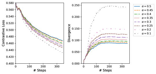
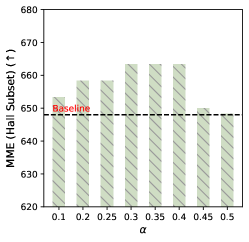
(a) The training curves with varying $\alpha$.	(b) Performance on MME-Hall. with varying $\alpha$.

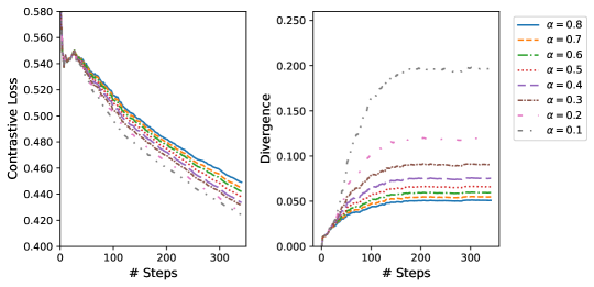
Figure S1: The training curves with varying $\alpha$ (a) and their performance on object hallucination (b) are presented. $\alpha$ in the range of 0.1 to 0.4 achieves optimal performance on the 7B variant.

(a) The training curves with varying $\alpha$.	(b) Performance on MME-Hall. with varying $\alpha$.

Figure S2: The training curves with varying $\alpha$ (a) and their performance on object hallucination (b) are presented. $\alpha$ in the range of 0.4 to 0.6 achieves optimal performance on the 13B variant.

Figure S3: Qualitative examples demonstrating the impact of contrastive tuning with a very low $\alpha$. As presented here, training with a very low $\alpha$ of 0.01 may hurt the language generation ability of an MLLM. The example on the left side shows an instance of degeneration, while the example on the right side shows a lack of descriptive power, failing to mention key details in the description, such as ‘the man is wearing a tie’ or ‘the girl is wearing a dress’. The 7B variant is used in this study.

B.2 Ablation on Generative Data Augmentation

We perform an ablation study to explore the effect of different sampling strategies which have been used in generative data augmentation. As mentioned in Section 2, we generate hallucinated responses in three setups: closed-set co-occurrences (9K), open-set co-occurrences (11K), and Yes-or-No questions (1.5K). We study the impact of these categories along with their varying number of samples. We perform this study on HALVA${}_{\text{7B}}$ and use the same training hyperparameters as those obtained by tuning on the entire data. From the results presented in Table S1, three key observations are made. First, open-set hallucinated descriptions show benefits in reducing hallucinations in generative tasks, as evidenced by the superior performance on CHAIR. Second, mixing the Yes-or-No hallucinated responses reduces hallucination in discriminative tasks, leading to an F1 boost on the AMBER dataset. Finally, combining all the splits results in overall improvements or competitive performances across a broader range of tasks.

Table S1: Ablation study on sampling strategy used in generative data augmentation. $C_{i}$ and $C_{s}$ refer to CHAIR at instance and sentence-level; F1 refers to the F1-scores of all the discriminative tasks and HR refers to hallucination rate on generative tasks.

Data Split	# Samples	CHAIR		AMBER		MME-Hall
		C${}_{i}\downarrow$	C${}_{s}\downarrow$	F1$\uparrow$	HR $\downarrow$	Score $\uparrow$
Closed set	9K	12.6	45.0	73.9	34.7	643.3
Open-set	11K	11.2	39.6	73.1	33.3	643.3
Closed set + Open-set (50%)	10K	11.7	41.8	79.8	32.0	643.3
Closed set + Open-set	20K	12.6	43.6	74.1	34.0	648.3
Closed set + Open-set + Y-or-N (50%)	11K	11.8	43.2	82.4	32.2	641.0
Closed set + Open-set + Y-or-N	21.5K	11.7	41.4	83.4	32.2	665.0

Table S2: Ablation study on divergence measure using HALVA${}_{\text{7B}}$. (a) We find that using seen samples as the reference data for divergence measure achieve overall better performance. (b) Our study shows that initializing the reference model and the model being trained from the same checkpoint, achieves optimal performance. $C_{i}$ and $C_{s}$ refer to CHAIR at instance and sentence-level; F1 refers to the F1-scores of all the discriminative tasks and HR refers to hallucination rate in the image descriptions.

(a) Ablation study on reference data.

Ref. Data	CHAIR		AMBER		MME-Hall
	C${}_{i}\downarrow$	C${}_{s}\downarrow$	F1$\uparrow$	HR $\downarrow$	Score $\uparrow$
Unseen data	12.7	47.4	81.7	34.7	668.3
Seen data	11.7	41.4	83.4	32.2	665.0

(b) Ablation study on reference model.

Ref. Model	CHAIR		AMBER		MME-Hall
	C${}_{i}\downarrow$	C${}_{s}\downarrow$	F1$\uparrow$	HR $\downarrow$	Score $\uparrow$
7B	11.7	41.4	83.4	32.2	665.0
13B	12.4	45.2	80.1	34.7	640.0

B.3 Ablation on Divergence Measure

Reference Data. We experiment with the reference data that has been used to measure KL divergence with respect to the reference model. We briefly experiment in two setups:

• Unseen data: we directly use the vision-language instructions and correct descriptions of the contrastive response pairs as the reference samples.

• Seen data: we take a fraction of the instruction tuning dataset LLaVA-v1.5 is originally trained on, and use them as reference samples.

We perform this experiment on HALVA${}_{\text{7B}}$ and the results are presented in Table B.2 (a). The results demonstrate that using seen samples to measure divergence gives a better estimate of model state during training, and accordingly the tuned model overall performs better, across various benchmarks.

Reference Model. By default, we initialize the reference model (the model kept frozen) and the online model (the model being trained) from the same checkpoint. Additionally, we experiment with initializing the reference model different than the model being trained. In particular, we experiment with training LLaVA${}_{\text{7B}}$ while using LLaVA${}_{\text{13B}}$ as the reference model. We find this interesting to explore as both LLaVA${}_{\text{7B}}$ and LLaVA${}_{\text{13B}}$ are originally trained in a similar setup, and LLaVA${}_{\text{13B}}$ performs relatively better compared to the LLaVA${}_{\text{7B}}$, on most of the benchmarks [9]. The results presented in Table B.2 (b) show that initializing the reference model and the online model from the same checkpoint, achieve optimal performance. We believe this is likely since the reference model initialized from an identical state of the model being trained, gives a true estimate of divergence and accordingly optimized model performs better across a variety of benchmarks.

B.4 Detailed Results of MME (Hallucination Subset)

In Table S3, we present the detailed results of the MME-Hall [44] benchmark across its four sub-categories: existence, count, position, and color. Our results indicate that contrastive tuning improves (or retains) object hallucination across different aspects, unlike prior work such as HA-DPO [26] or VCD [20], which show improvement in one category but suffer in others.

Table S3: Detailed results on MME-Hall.

Method	Object $(\uparrow)$			Attribute $(\uparrow)$		Total $(\uparrow)$
	Existence	Count		Position	Color
LLaVA-v1.5${}_{\text{7B}}$	190.0	155.0		133.3	170.0	648.3
LLaVA-v1.5${}_{\text{7B}}$ w/ HA-DPO	190.0	133.3		136.7	158.3	618.3
LLaVA-v1.5${}_{\text{7B}}$ w/ EOS	190.0	138.3		118.3	160.0	606.7
LLaVA-v1.5${}_{\text{7B}}$ w/ VCD	184.7	138.3		128.7	153.0	604.7
HALVA${}_{\text{7B}}$ (Ours)	190.0	165.0		135.0	175.0	665.0
LLaVA-v1.5${}_{\text{13B}}$	185.0	155.0		133.3	170.0	643.3
HALVA${}_{\text{13B}}$ (Ours)	190.0	163.3		141.7	180.0	675.0

B.5 Detailed Results of MMHal-Bench

In Table S4, we present the detailed results of MMHal-Bench [24] across its eight sub-categories. Our contrastive tuning demonstrates consistent effectiveness in mitigating object hallucinations in the following types: adversarial, comparison, relation, and holistic on both HALVA${}_{\text{7B}}$ and HALVA${}_{\text{13B}}$. Moreover, recent hallucination mitigation methods such as HA-DPO and EOS prove ineffective in addressing such broad categories of hallucinations, even resulting in worsened baseline performance.

Table S4: Detailed results on MMHal-Bench.

Method	Overall	Hall.	Score in Each Question Type $(\uparrow)$
	Score $(\uparrow)$	Rate $\mathbf{(\downarrow)}$	Attribute	Adversarial	Comparison	Counting	Relation	Environment	Holistic	Other
LLaVA-v1.5${}_{\textsc{7B}}$	2.11±0.06	0.56±0.01	3.06±0.27	1.00±0.00	1.61±0.05	1.97±0.09	2.36±0.05	3.20±0.05	2.14±0.30	1.53±0.25
LLaVA-v1.5 w/ HA-DPO${}_{\text{7B}}$	1.97±0.04	0.59±0.01	3.56±0.17	1.08±0.09	1.14±0.13	1.89±0.21	2.22±0.33	3.31±0.10	1.42±0.14	1.17±0.00
LLaVA-v1.5 w/ EOS${}_{\text{7B}}$	2.03±0.02	0.59±0.02	2.69±0.13	1.78±0.09	1.89±0.13	1.53±0.18	2.09±0.14	3.08±0.30	1.67±0.29	1.53±0.09
HALVA${}_{\text{7B}}$ (Ours)	2.25±0.10	0.54±0.01	2.78±0.09	1.47±0.18	1.97±0.13	1.89±0.05	3.03±0.21	3.20±0.05	2.42±0.43	1.22±0.27
LLaVA-v1.5${}_{\text{13B}}$	2.38±0.02	0.50±0.01	3.20±0.05	2.53±0.18	2.55±0.05	2.20±0.05	1.97±0.05	3.33±0.14	1.50±0.22	1.72±0.13
HALVA${}_{\text{13B}}$ (Ours)	2.58±0.08	0.46±0.02	3.03±0.09	2.58±0.09	2.66±0.14	2.08±0.14	2.45±0.05	3.36±0.17	2.44±0.39	2.00±0.08

B.6 Detailed Results of HallusionBench

In Table S5, we present the detailed results of HallusionBench [46], which evaluates MLLMs beyond object hallucination, including those may cause by visual illusions and quantitative analysis form charts or graphs, among others. In addition to improving the overall performance, the results demonstrate the effectiveness of contrastive tuning on all the sub-categories (i.e., easy set, hard set) of HallusionBench as well. We note that, in addition to hallucination mitigation, our contrastive tuning helps MLLMs in reducing Yes/No bias. As discussed earlier, LLaVA-v1.5 is prone to answering ‘Yes’, in most cases. Our contrastive tuning effectively reduces Yes/No bias from 0.31 to 0.17 and from 0.38 to 0.20 on HALVA${}_{\text{7B}}$ and HALVA${}_{\text{13B}}$, respectively.

Table S5: Detailed results on HallusionBench.

Method	Yes/No Bias		Question Pair Acc.	Fig. Acc.	Easy Acc.	Hard Acc.	All Acc.
	Pct. Diff ($\sim 0$)	FP Ratio ($\sim 0.5$)	(qAcc) $\uparrow$	(fAcc) $\uparrow$	(Easy aAcc) $\uparrow$	(Hard aAcc) $\uparrow$	(aAcc) $\uparrow$
LLaVA-v1.5${}^{*}_{\text{7B}}$	0.31±0.00	0.79±0.00	10.70±0.13	19.65±0.00	42.34±0.13	41.47±0.13	47.09±0.14
HALVA${}_{\text{7B}}$ (Ours)	0.17±0.00	0.67±0.00	13.85±0.00	21.48±0.17	42.71±0.13	45.81±0.00	48.95±0.14
LLaVA-v1.5${}_{\text{13B}}$	0.38±0.00	0.85±0.00	8.79±0.22	15.22±0.17	44.25±0.13	35.97±0.13	46.50±0.09
HALVA${}_{\text{13B}}$ (Ours)	0.20±0.00	0.70±0.00	13.85±0.22	20.13±0.17	44.47±0.13	42.87±0.13	49.10±0.05

B.7 A Critical Analysis of Contrastive Tuning

Here, we critically assess whether the performance enhancement observed in our proposed contrastive tuning is attributable to generative data augmentation, the proposed contrastive objective, or their combination. To investigate this, we apply our generative data augmentation directly to another finetuning-based hallucination mitigation approach, HA-DPO [26]. In HA-DPO, contrastive pairs are employed to finetune MLLMs, aiming to maximize the reward margin between the correct responses and the hallucinated ones. Accordingly, we train HA-DPO by replacing their data with the output of our generative data augmentation module. We utilize the official code released by [26] and conduct hyper-parameter tuning (mainly with varying $\beta$ and learning rate) ensure effective training. Subsequently, we evaluate the performance of the newly trained HA-DPO on both hallucination (CHAIR, AMBER, MME-Hall) and non-hallucination (MME) benchmarks. The results presented in Table S6 indicate that applying our proposed generative data augmentation to HA-DPO does not yield the same level of performance boost as HALVA. This confirms that the performance boost of our proposed method stems from a combination of the contrastive objective and the data augmentation setup. Note that since our proposed method necessitates a pair of correct and hallucinated tokens to apply contrastive tuning, and the descriptive responses utilized in HA-DPO do not meet this requirement, we are unable to apply our contrastive tuning directly to their data.

Table S6: Effect of generative data augmentation on HA-DPO. Here, CHAIR, AMBER, and MME-Hall are hallucination benchmarks, and MME is a general vision-language benchmark.

	CHAIR (Ci) $\downarrow$	AMBER F1 $\uparrow$	MME-Hall $\uparrow$	MME $\uparrow$
LLaVA-v1.5${}_{\text{7B}}$	15.4	74.7	648.3	1510.7
HA-DPO${}_{\text{7B}}$	11.0	78.1	618.3	1502.6
HA-DPO${}_{\text{7B}}$ w/ Generative Data Aug.	14.6	77.7	631.7	1508.9
HALVA${}_{\text{7B}}$	11.7	83.4	665.0	1527.0

Appendix C Implementation Details

C.1 Training Hyperparameters

The details of training hyperparameters used in contrastive tuning is presented in Table S7.

Table S7: Details of training hyperparameters used in contrastive tuning.

	HALVA${}_{\text{7B}}$	HALVA${}_{\text{13B}}$
Base model	LLaVA-v1.5${}_{\text{7B}}$ [9]	LLaVA-v1.5${}_{\text{13B}}$ [9]
LLM	Vicuna-v1.5${}_{\text{7B}}$ [41, 5]	Vicuna-v1.5${}_{\text{13B}}$ [41, 5]
Vision encoder	CLIP ViT-L336/14 [42]
Trainable module	LoRA in LLM and everything else is kept frozen
LoRA setup [43]	rank=128, alpha=256
Learning rate	5e-6
Learning rate scheduler	Cosine
Optimizer	AdamW [76]
Weight decay	0.
Warmup ratio	0.03
Epoch	1 (342 steps)
Batch size per GPU	16
Batch size (total)	64
$\alpha$ (loss coefficient)	0.4	0.5
Memory optimization	Zero stage 3 [77, 78]
Training time	1.5 hrs	3 hrs.

C.2 Licenses of Existing Assets Used

For images, we use publicly-available Visual Genome dataset [40]. This dataset can be downloaded from https://homes.cs.washington.edu/~ranjay/visualgenome/api.html and is licensed under a Creative Commons Attribution 4.0 International License.

For the base MLLM, we use LLaVA-v1.5 [9] which is publicly available and its Apache license 2.0 can be found at https://github.com/haotian-liu/LLaVA/blob/main/LICENSE.

C.3 Generative Data Augmentation Setup

We present the prompt templates that are used to prepare correct and hallucinated descriptions in Figures S4-S7. We leverage Gemini Vision Pro (gemini-1.0-pro-vision) in preparing the responses. We present examples of training samples in Figures S8-S11.

Figure S4: The template for generating the correct image descriptions.

Figure S5: The template for generating the closed-set hallucinated descriptions.

Figure S6: The template for generating the open-set hallucinated descriptions.

Figure S7: Instructions for different types of image descriptions. These instructions are directly taken from [8], we list them here for the sake of completeness.

Figure S8: Examples of one sentence captions used in contrastive tuning.

Figure S9: Examples of short image descriptions used in contrastive tuning.

Figure S10: Examples of detailed image descriptions used in contrastive tuning.

Figure S11: Examples of Yes-or-No questions used in contrastive tuning.

Appendix D Qualitative results

Figure S12: Comparing detailed image descriptions between HALVA ()  and its base model LLaVA-v1.5 (). Unlike HALVA, LLaVA-v1.5 hallucinates ‘carrot’ in the image description. Hallucinations are highlighted in red.

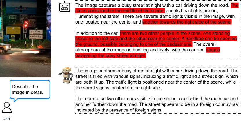
Figure S13: Comparing detailed image descriptions between HALVA ()  and its base model LLaVA-v1.5 (). LLaVA-v1.5 wrongfully describes the position of the ‘cars’ and ‘traffic lights’. Moreover, it hallucinates the presence of ‘people’, ‘pedestrian’, and ‘handbag’. In contrast, HALVA correctly identifies the relative positions of the ‘traffic lights’ and ‘cars’, while accurately describing the image. Hallucinations are highlighted in red.

Figure S14: Comparing detailed image descriptions between HALVA ()  and its base model LLaVA-v1.5 (). LLaVA-v1.5 exhibits object hallucination that may happen due to object co-occurrence in the training data, such as the occurrence of ‘pitcher’ with ‘batter’, ‘catcher’, and ‘umpire’. HALVA effectively mitigates such hallucination and accurately describes the image with necessary details. Hallucinations are highlighted in red.

Figure S15: HALVA () does not exhibit a tendency to answer ‘Yes’ for any questions asked, like LLaVA-v1.5 (). Moreover, HALVA can accurately lay out the details of the image to further support the answer. As presented in the right side example, HALVA answers with “the dog is not directly touching the sea. It is running on the beach near the water, but there is a gap between the dog and the water.”. Hallucinations are highlighted in red.

Figure S16: HALVA () does not exhibit a tendency to answer ‘Yes’ for any questions asked, like LLaVA-v1.5 (). Moreover, HALVA exhibit consistency in its response unlike LLaVA-v1.5. Hallucinations are highlighted in red.

References

- [1] Aakanksha Chowdhery, Sharan Narang, Jacob Devlin, Maarten Bosma, Gaurav Mishra, Adam Roberts, Paul Barham, Hyung Won Chung, Charles Sutton, Sebastian Gehrmann, et al. Palm: Scaling language modeling with pathways. JMLR, 24(240):1–113, 2023.
- [2] Rohan Anil, Andrew M Dai, Orhan Firat, Melvin Johnson, Dmitry Lepikhin, Alexandre Passos, Siamak Shakeri, Emanuel Taropa, Paige Bailey, Zhifeng Chen, et al. Palm 2 technical report. arXiv preprint arXiv:2305.10403, 2023.
- [3] Colin Raffel, Noam Shazeer, Adam Roberts, Katherine Lee, Sharan Narang, Michael Matena, Yanqi Zhou, Wei Li, and Peter J. Liu. Exploring the limits of transfer learning with a unified text-to-text transformer. JMLR, 21(140):1–67, 2020.
- [4] Hugo Touvron, Thibaut Lavril, Gautier Izacard, Xavier Martinet, Marie-Anne Lachaux, Timothée Lacroix, Baptiste Rozière, Naman Goyal, Eric Hambro, Faisal Azhar, et al. Llama: Open and efficient foundation language models. arXiv preprint arXiv:2302.13971, 2023.
- [5] Hugo Touvron, Louis Martin, Kevin Stone, Peter Albert, Amjad Almahairi, Yasmine Babaei, Nikolay Bashlykov, Soumya Batra, Prajjwal Bhargava, Shruti Bhosale, et al. Llama 2: Open foundation and fine-tuned chat models. arXiv preprint arXiv:2307.09288, 2023.
- [6] Gemini Team, Rohan Anil, Sebastian Borgeaud, Yonghui Wu, Jean-Baptiste Alayrac, Jiahui Yu, Radu Soricut, Johan Schalkwyk, Andrew M Dai, Anja Hauth, et al. Gemini: a family of highly capable multimodal models. arXiv preprint arXiv:2312.11805, 2023.
- [7] Tom Brown, Benjamin Mann, Nick Ryder, Melanie Subbiah, Jared D Kaplan, Prafulla Dhariwal, Arvind Neelakantan, Pranav Shyam, Girish Sastry, Amanda Askell, et al. Language models are few-shot learners. NeurIPS, 33:1877–1901, 2020.
- [8] Haotian Liu, Chunyuan Li, Qingyang Wu, and Yong Jae Lee. Visual instruction tuning. NeurIPS, 36, 2024.
- [9] Haotian Liu, Chunyuan Li, Yuheng Li, and Yong Jae Lee. Improved baselines with visual instruction tuning. arXiv preprint arXiv:2310.03744, 2023.
- [10] Wenliang Dai, Junnan Li, Dongxu Li, Anthony Meng Huat Tiong, Junqi Zhao, Weisheng Wang, Boyang Li, Pascale Fung, and Steven Hoi. Instructblip: Towards general-purpose vision-language models with instruction tuning. arXiv preprint arXiv:2305.06500, 2023.
- [11] Junnan Li, Dongxu Li, Silvio Savarese, and Steven Hoi. Blip-2: Bootstrapping language-image pre-training with frozen image encoders and large language models. arXiv preprint arXiv:2301.12597, 2023.
- [12] Josh Achiam, Steven Adler, Sandhini Agarwal, Lama Ahmad, Ilge Akkaya, Florencia Leoni Aleman, Diogo Almeida, Janko Altenschmidt, Sam Altman, Shyamal Anadkat, et al. Gpt-4 technical report. arXiv preprint arXiv:2303.08774, 2023.
- [13] Sheng Wang, Zihao Zhao, Xi Ouyang, Qian Wang, and Dinggang Shen. Chatcad: Interactive computer-aided diagnosis on medical image using large language models. arXiv preprint arXiv:2302.07257, 2023.
- [14] Mingzhe Hu, Shaoyan Pan, Yuheng Li, and Xiaofeng Yang. Advancing medical imaging with language models: A journey from n-grams to chatgpt. arXiv preprint arXiv:2304.04920, 2023.
- [15] Anna Rohrbach, Lisa Anne Hendricks, Kaylee Burns, Trevor Darrell, and Kate Saenko. Object hallucination in image captioning. arXiv preprint arXiv:1809.02156, 2018.
- [16] Zechen Bai, Pichao Wang, Tianjun Xiao, Tong He, Zongbo Han, Zheng Zhang, and Mike Zheng Shou. Hallucination of multimodal large language models: A survey. arXiv preprint arXiv:2404.18930, 2024.
- [17] Fuxiao Liu, Kevin Lin, Linjie Li, Jianfeng Wang, Yaser Yacoob, and Lijuan Wang. Mitigating hallucination in large multi-modal models via robust instruction tuning. In ICLR, 2023.
- [18] Ailin Deng, Zhirui Chen, and Bryan Hooi. Seeing is believing: Mitigating hallucination in large vision-language models via clip-guided decoding. arXiv preprint arXiv:2402.15300, 2024.
- [19] Shukang Yin, Chaoyou Fu, Sirui Zhao, Tong Xu, Hao Wang, Dianbo Sui, Yunhang Shen, Ke Li, Xing Sun, and Enhong Chen. Woodpecker: Hallucination correction for multimodal large language models. arXiv preprint arXiv:2310.16045, 2023.
- [20] Sicong Leng, Hang Zhang, Guanzheng Chen, Xin Li, Shijian Lu, Chunyan Miao, and Lidong Bing. Mitigating object hallucinations in large vision-language models through visual contrastive decoding. arXiv preprint arXiv:2311.16922, 2023.
- [21] Seongyun Lee, Sue Hyun Park, Yongrae Jo, and Minjoon Seo. Volcano: mitigating multimodal hallucination through self-feedback guided revision. arXiv preprint arXiv:2311.07362, 2023.
- [22] Yiyang Zhou, Chenhang Cui, Jaehong Yoon, Linjun Zhang, Zhun Deng, Chelsea Finn, Mohit Bansal, and Huaxiu Yao. Analyzing and mitigating object hallucination in large vision-language models. arXiv preprint arXiv:2310.00754, 2023.
- [23] Ali Furkan Biten, Lluís Gómez, and Dimosthenis Karatzas. Let there be a clock on the beach: Reducing object hallucination in image captioning. In WACV, pages 1381–1390, 2022.
- [24] Zhiqing Sun, Sheng Shen, Shengcao Cao, Haotian Liu, Chunyuan Li, Yikang Shen, Chuang Gan, Liang-Yan Gui, Yu-Xiong Wang, Yiming Yang, et al. Aligning large multimodal models with factually augmented rlhf. arXiv preprint arXiv:2309.14525, 2023.
- [25] Chaoya Jiang, Haiyang Xu, Mengfan Dong, Jiaxing Chen, Wei Ye, Ming Yan, Qinghao Ye, Ji Zhang, Fei Huang, and Shikun Zhang. Hallucination augmented contrastive learning for multimodal large language model. arXiv preprint arXiv:2312.06968, 2023.
- [26] Zhiyuan Zhao, Bin Wang, Linke Ouyang, Xiaoyi Dong, Jiaqi Wang, and Conghui He. Beyond hallucinations: Enhancing lvlms through hallucination-aware direct preference optimization. arXiv preprint arXiv:2311.16839, 2023.
- [27] Zihao Yue, Liang Zhang, and Qin Jin. Less is more: Mitigating multimodal hallucination from an eos decision perspective. arXiv preprint arXiv:2402.14545, 2024.
- [28] Lanyun Zhu, Deyi Ji, Tianrun Chen, Peng Xu, Jieping Ye, and Jun Liu. Ibd: Alleviating hallucinations in large vision-language models via image-biased decoding. arXiv preprint arXiv:2402.18476, 2024.
- [29] Junfei Wu, Qiang Liu, Ding Wang, Jinghao Zhang, Shu Wu, Liang Wang, and Tieniu Tan. Logical closed loop: Uncovering object hallucinations in large vision-language models. arXiv preprint arXiv:2402.11622, 2024.
- [30] Tianyu Yu, Yuan Yao, Haoye Zhang, Taiwen He, Yifeng Han, Ganqu Cui, Jinyi Hu, Zhiyuan Liu, Hai-Tao Zheng, Maosong Sun, et al. Rlhf-v: Towards trustworthy mllms via behavior alignment from fine-grained correctional human feedback. arXiv preprint arXiv:2312.00849, 2023.
- [31] Assaf Ben-Kish, Moran Yanuka, Morris Alper, Raja Giryes, and Hadar Averbuch-Elor. Mocha: Multi-objective reinforcement mitigating caption hallucinations. arXiv preprint arXiv:2312.03631, 2023.
- [32] Yao Qin, Chiyuan Zhang, Ting Chen, Balaji Lakshminarayanan, Alex Beutel, and Xuezhi Wang. Understanding and improving robustness of vision transformers through patch-based negative augmentation. NeurIPS, 35:16276–16289, 2022.
- [33] Chenyu Zheng, Guoqiang Wu, and Chongxuan Li. Toward understanding generative data augmentation. NeurIPS, 36, 2024.
- [34] Paul F Christiano, Jan Leike, Tom Brown, Miljan Martic, Shane Legg, and Dario Amodei. Deep reinforcement learning from human preferences. NeurIPS, 30, 2017.
- [35] Rafael Rafailov, Archit Sharma, Eric Mitchell, Christopher D Manning, Stefano Ermon, and Chelsea Finn. Direct preference optimization: Your language model is secretly a reward model. NeurIPS, 36, 2024.
- [36] Jonathon Shlens. Notes on kullback-leibler divergence and likelihood. arXiv preprint arXiv:1404.2000, 2014.
- [37] Yifan Li, Yifan Du, Kun Zhou, Jinpeng Wang, Wayne Xin Zhao, and Ji-Rong Wen. Evaluating object hallucination in large vision-language models. arXiv preprint arXiv:2305.10355, 2023.
- [38] Rico Sennrich, Barry Haddow, and Alexandra Birch. Neural machine translation of rare words with subword units. arXiv preprint arXiv:1508.07909, 2015.
- [39] Taku Kudo and John Richardson. Sentencepiece: A simple and language independent subword tokenizer and detokenizer for neural text processing. arXiv preprint arXiv:1808.06226, 2018.
- [40] Ranjay Krishna, Yuke Zhu, Oliver Groth, Justin Johnson, Kenji Hata, Joshua Kravitz, Stephanie Chen, Yannis Kalantidis, Li-Jia Li, David A Shamma, et al. Visual genome: Connecting language and vision using crowdsourced dense image annotations. IJCV, 123:32–73, 2017.
- [41] Wei-Lin Chiang, Zhuohan Li, Zi Lin, Ying Sheng, Zhanghao Wu, Hao Zhang, Lianmin Zheng, Siyuan Zhuang, Yonghao Zhuang, Joseph E. Gonzalez, Ion Stoica, and Eric P. Xing. Vicuna: An open-source chatbot impressing gpt-4 with 90%* chatgpt quality, March 2023.
- [42] Alec Radford, Jong Wook Kim, Chris Hallacy, Aditya Ramesh, Gabriel Goh, Sandhini Agarwal, Girish Sastry, Amanda Askell, Pamela Mishkin, Jack Clark, et al. Learning transferable visual models from natural language supervision. In ICML, pages 8748–8763. PMLR, 2021.
- [43] Edward J Hu, Yelong Shen, Phillip Wallis, Zeyuan Allen-Zhu, Yuanzhi Li, Shean Wang, Lu Wang, and Weizhu Chen. Lora: Low-rank adaptation of large language models. arXiv preprint arXiv:2106.09685, 2021.
- [44] Chaoyou Fu, Peixian Chen, Yunhang Shen, Yulei Qin, Mengdan Zhang, Xu Lin, Jinrui Yang, Xiawu Zheng, Ke Li, Xing Sun, Yunsheng Wu, and Rongrong Ji. Mme: A comprehensive evaluation benchmark for multimodal large language models. arXiv preprint arXiv:2306.13394, 2023.
- [45] Junyang Wang, Yuhang Wang, Guohai Xu, Jing Zhang, Yukai Gu, Haitao Jia, Ming Yan, Ji Zhang, and Jitao Sang. An llm-free multi-dimensional benchmark for mllms hallucination evaluation. arXiv preprint arXiv:2311.07397, 2023.
- [46] Fuxiao Liu, Tianrui Guan, Zongxia Li, Lichang Chen, Yaser Yacoob, Dinesh Manocha, and Tianyi Zhou. Hallusionbench: You see what you think? or you think what you see? an image-context reasoning benchmark challenging for gpt-4v (ision), llava-1.5, and other multi-modality models. arXiv preprint arXiv:2310.14566, 2023.
- [47] Yash Goyal, Tejas Khot, Douglas Summers-Stay, Dhruv Batra, and Devi Parikh. Making the v in vqa matter: Elevating the role of image understanding in visual question answering. In CVPR, pages 6904–6913, 2017.
- [48] Weihao Yu, Zhengyuan Yang, Linjie Li, Jianfeng Wang, Kevin Lin, Zicheng Liu, Xinchao Wang, and Lijuan Wang. Mm-vet: Evaluating large multimodal models for integrated capabilities. arXiv preprint arXiv:2308.02490, 2023.
- [49] Amanpreet Singh, Vivek Natarajan, Meet Shah, Yu Jiang, Xinlei Chen, Dhruv Batra, Devi Parikh, and Marcus Rohrbach. Towards vqa models that can read. In CVPR, pages 8317–8326, 2019.
- [50] Qidong Huang, Xiaoyi Dong, Pan Zhang, Bin Wang, Conghui He, Jiaqi Wang, Dahua Lin, Weiming Zhang, and Nenghai Yu. Opera: Alleviating hallucination in multi-modal large language models via over-trust penalty and retrospection-allocation. arXiv preprint arXiv:2311.17911, 2023.
- [51] Jun Chen, Deyao Zhu, Xiaoqian Shen, Xiang Li, Zechun Liu, Pengchuan Zhang, Raghuraman Krishnamoorthi, Vikas Chandra, Yunyang Xiong, and Mohamed Elhoseiny. Minigpt-v2: large language model as a unified interface for vision-language multi-task learning. arXiv preprint arXiv:2310.09478, 2023.
- [52] Qinghao Ye, Haiyang Xu, Guohai Xu, Jiabo Ye, Ming Yan, Yiyang Zhou, Junyang Wang, Anwen Hu, Pengcheng Shi, Yaya Shi, et al. mplug-owl: Modularization empowers large language models with multimodality. arXiv preprint arXiv:2304.14178, 2023.
- [53] Tao Gong, Chengqi Lyu, Shilong Zhang, Yudong Wang, Miao Zheng, Qian Zhao, Kuikun Liu, Wenwei Zhang, Ping Luo, and Kai Chen. Multimodal-gpt: A vision and language model for dialogue with humans. arXiv preprint arXiv:2305.04790, 2023.
- [54] Deyao Zhu, Jun Chen, Xiaoqian Shen, Xiang Li, and Mohamed Elhoseiny. Minigpt-4: Enhancing vision-language understanding with advanced large language models. arXiv preprint arXiv:2304.10592, 2023.
- [55] Juncheng Li, Kaihang Pan, Zhiqi Ge, Minghe Gao, Hanwang Zhang, Wei Ji, Wenqiao Zhang, Tat-Seng Chua, Siliang Tang, and Yueting Zhuang. Empowering vision-language models to follow interleaved vision-language instructions. arXiv preprint arXiv:2308.04152, 2023.
- [56] Bo Li, Yuanhan Zhang, Liangyu Chen, Jinghao Wang, Fanyi Pu, Jingkang Yang, Chunyuan Li, and Ziwei Liu. Mimic-it: Multi-modal in-context instruction tuning. arXiv preprint arXiv:2306.05425, 2023.
- [57] Qinghao Ye, Haiyang Xu, Jiabo Ye, Ming Yan, Haowei Liu, Qi Qian, Ji Zhang, Fei Huang, and Jingren Zhou. mplug-owl2: Revolutionizing multi-modal large language model with modality collaboration. arXiv preprint arXiv:2311.04257, 2023.
- [58] Yan Zeng, Hanbo Zhang, Jiani Zheng, Jiangnan Xia, Guoqiang Wei, Yang Wei, Yuchen Zhang, and Tao Kong. What matters in training a gpt4-style language model with multimodal inputs? arXiv preprint arXiv:2307.02469, 2023.
- [59] Jinze Bai, Shuai Bai, Shusheng Yang, Shijie Wang, Sinan Tan, Peng Wang, Junyang Lin, Chang Zhou, and Jingren Zhou. Qwen-vl: A versatile vision-language model for understanding, localization, text reading, and beyond. 2023.
- [60] Peng Gao, Jiaming Han, Renrui Zhang, Ziyi Lin, Shijie Geng, Aojun Zhou, Wei Zhang, Pan Lu, Conghui He, Xiangyu Yue, et al. Llama-adapter v2: Parameter-efficient visual instruction model. arXiv preprint arXiv:2304.15010, 2023.
- [61] Wenbo Hu, Yifan Xu, Yi Li, Weiyue Li, Zeyuan Chen, and Zhuowen Tu. Bliva: A simple multimodal llm for better handling of text-rich visual questions. In AAAI, volume 38, pages 2256–2264, 2024.
- [62] Haozhe Zhao, Zefan Cai, Shuzheng Si, Xiaojian Ma, Kaikai An, Liang Chen, Zixuan Liu, Sheng Wang, Wenjuan Han, and Baobao Chang. Mmicl: Empowering vision-language model with multi-modal in-context learning. arXiv preprint arXiv:2309.07915, 2023.
- [63] Ziyi Lin, Chris Liu, Renrui Zhang, Peng Gao, Longtian Qiu, Han Xiao, Han Qiu, Chen Lin, Wenqi Shao, Keqin Chen, et al. Sphinx: The joint mixing of weights, tasks, and visual embeddings for multi-modal large language models. arXiv preprint arXiv:2311.07575, 2023.
- [64] Renze Lou, Kai Zhang, Jian Xie, Yuxuan Sun, Janice Ahn, Hanzi Xu, Yu Su, and Wenpeng Yin. Muffin: Curating multi-faceted instructions for improving instruction following. In ICLR, 2023.
- [65] Zhiliang Peng, Wenhui Wang, Li Dong, Yaru Hao, Shaohan Huang, Shuming Ma, and Furu Wei. Kosmos-2: Grounding multimodal large language models to the world. arXiv preprint arXiv:2306.14824, 2023.
- [66] Hugo Laurençon, Lucile Saulnier, Léo Tronchon, Stas Bekman, Amanpreet Singh, Anton Lozhkov, Thomas Wang, Siddharth Karamcheti, Alexander Rush, Douwe Kiela, et al. Obelics: An open web-scale filtered dataset of interleaved image-text documents. NeurIPS, 36, 2024.
- [67] Kaizhi Zheng, Xuehai He, and Xin Eric Wang. Minigpt-5: Interleaved vision-and-language generation via generative vokens. arXiv preprint arXiv:2310.02239, 2023.
- [68] Anas Awadalla, Irena Gao, Josh Gardner, Jack Hessel, Yusuf Hanafy, Wanrong Zhu, Kalyani Marathe, Yonatan Bitton, Samir Gadre, Shiori Sagawa, et al. Openflamingo: An open-source framework for training large autoregressive vision-language models. arXiv preprint arXiv:2308.01390, 2023.
- [69] Chao Jia, Yinfei Yang, Ye Xia, Yi-Ting Chen, Zarana Parekh, Hieu Pham, Quoc Le, Yun-Hsuan Sung, Zhen Li, and Tom Duerig. Scaling up visual and vision-language representation learning with noisy text supervision. In ICML, pages 4904–4916. PMLR, 2021.
- [70] Jiahui Yu, Zirui Wang, Vijay Vasudevan, Legg Yeung, Mojtaba Seyedhosseini, and Yonghui Wu. Coca: Contrastive captioners are image-text foundation models. arXiv preprint arXiv:2205.01917, 2022.
- [71] Xi Chen, Xiao Wang, Soravit Changpinyo, AJ Piergiovanni, Piotr Padlewski, Daniel Salz, Sebastian Goodman, Adam Grycner, Basil Mustafa, Lucas Beyer, et al. Pali: A jointly-scaled multilingual language-image model. arXiv preprint arXiv:2209.06794, 2022.
- [72] Junnan Li, Dongxu Li, Caiming Xiong, and Steven Hoi. Blip: Bootstrapping language-image pre-training for unified vision-language understanding and generation. In ICML, pages 12888–12900. PMLR, 2022.
- [73] Peng Wang, An Yang, Rui Men, Junyang Lin, Shuai Bai, Zhikang Li, Jianxin Ma, Chang Zhou, Jingren Zhou, and Hongxia Yang. Ofa: Unifying architectures, tasks, and modalities through a simple sequence-to-sequence learning framework. In ICML, pages 23318–23340. PMLR, 2022.
- [74] Keqin Chen, Zhao Zhang, Weili Zeng, Richong Zhang, Feng Zhu, and Rui Zhao. Shikra: Unleashing multimodal llm’s referential dialogue magic. arXiv preprint arXiv:2306.15195, 2023.
- [75] Bin Wang, Fan Wu, Xiao Han, Jiahui Peng, Huaping Zhong, Pan Zhang, Xiaoyi Dong, Weijia Li, Wei Li, Jiaqi Wang, et al. Vigc: Visual instruction generation and correction. In AAAI, volume 38, pages 5309–5317, 2024.
- [76] Ilya Loshchilov and Frank Hutter. Decoupled weight decay regularization. arXiv preprint arXiv:1711.05101, 2017.
- [77] Jie Ren, Samyam Rajbhandari, Reza Yazdani Aminabadi, Olatunji Ruwase, Shuangyan Yang, Minjia Zhang, Dong Li, and Yuxiong He. Zero-offload: Democratizing billion-scale model training. In USENIX ATC, pages 551–564, 2021.
- [78] Samyam Rajbhandari, Olatunji Ruwase, Jeff Rasley, Shaden Smith, and Yuxiong He. Zero-infinity: Breaking the gpu memory wall for extreme scale deep learning. In SC, pages 1–14, 2021.