A semi-analytical thermal model for craters with application to the crater-induced YORP effect

Abstract

Context. The YORP effect is the thermal torque generated by radiation from the surface of an asteroid. The effect is sensitive to surface topology, including small-scale roughness, boulders, and craters.

Aims. The aim of this paper is to develop a computationally efficient semi-analytical model for the crater-induced YORP (CYORP) effect that can be used to investigate the functional dependence of this effect.

Methods. This study linearizes the thermal radiation term as a function of the temperature in the boundary condition of the heat conductivity, and obtains the temperature field in a crater over a rotational period in the form of a Fourier series, accounting for the effects of self-sheltering, self-radiation, and self-scattering. By comparison with a numerical model, we find that this semi-analytical model for the CYORP effect works well for $K>0.1\rm W/m/K$. This semi-analytical model is computationally three-orders-of-magnitude more efficient than the numerical approach.

Results. We obtain the temperature field of a crater, accounting for the thermal inertia, crater shape, and crater location. We then find that the CYORP effect is negligible when the depth-to-diameter ratio is smaller than 0.05. In this case, it is reasonable to assume a convex shape for YORP calculations. Varying the thermal conductivity yields a consistent value of approximately 0.01 for the spin component of the CYORP coefficient, while the obliquity component is inversely related to thermal inertia, declining from 0.004 in basalt to 0.001 in metal. The CYORP spin component peaks at an obliquity of $0^{\circ}$, $90^{\circ}$, or $180^{\circ}$, while the obliquity component peaks at an obliquity of around $45^{\circ}$ or $135^{\circ}$. For a z-axis symmetric shape, the CYORP spin component vanishes, while the obliquity component persists. Our model confirms that the total YORP torque is damped by a few tens of percent by uniformly distributed small-scale surface roughness. Furthermore, for the first time, we calculate the change in the YORP torque at each impact on the surface of an asteroid explicitly and compute the resulting stochastic spin evolution more precisely.

Conclusions. This study shows that the CYORP effect due to small-scale surface roughness and impact craters is significant during the history of asteroids. The semi-analytical method that we developed, which benefits from fast computation, offers new perspectives for future investigations of the YORP modeling of real asteroids and for the complete rotational and orbital evolution of asteroids accounting for collisions. Future research employing our CYORP model may explore the implications of space-varying roughness distribution, roughness in binary systems, and the development of a comprehensive rotational evolution model for asteroid groups.

1 Introduction

The Yarkovsky-O’Keefe-Radzievskii-Paddack (YORP) effect is a thermal torque that can alter the spin state of an asteroid over time (Rubincam 2000; Vokrouhlickỳ & Čapek 2002; Vokrouhlicky et al. 2015), and is caused by the asymmetric re-emission of solar radiation by the irregular surface of the asteroid, resulting in a net torque that can spin up or spin down the asteroid’s rotation. The absorption of solar radiation makes no contributions to the YORP torque as it is averaged out over the spin and orbital periods for any asteroid shapes (Nesvornỳ & Vokrouhlickỳ 2008). So far, 11 asteroids showing time-varying rotational periods have been detected (Lowry et al. 2007; Taylor et al. 2007; Ďurech et al. 2022; Tian et al. 2022).

The YORP effect has important implications for an asteroid’s long-term rotational evolution. This effect can either spin down the asteroid to an extremely slow rotation, triggering a tumbling motion (Pravec et al. 2005), or spin up the asteroid to its rotation limit (e.g. rotational period of 2.2 hours for rubble pile asteroids), leading to resurfacing (Sánchez & Scheeres 2020) and rotation disruption (Scheeres 2007; Fatka et al. 2020; Veras & Scheeres 2020). YORP-induced rotational disruption is supported by the observed asteroid pairs (Vokrouhlickỳ & Nesvornỳ 2008; Polishook 2014) and binary asteroids (Jacobson & Scheeres 2011; Delbo et al. 2011; Jacobson et al. 2013, 2016), including contact-binary asteroids (Rożek et al. 2019; Zegmott et al. 2021) and binary comets (Agarwal et al. 2020), which evolve under tidal effects and the binary YORP (BYORP) effect after the binary system is formed (Ćuk & Burns 2005; Steinberg et al. 2011). Further potential observational evidence is the abnormal spin distribution and the obliquity distribution of near-Earth asteroids (Vokrouhlickỳ et al. 2003; Pravec et al. 2008; Rozitis & Green 2013b; Lupishko & Tielieusova 2014) and main belt asteroids (Lupishko et al. 2019), although a recent study points out that collisions might reproduce the observed distribution without the involvement of the YORP effect (Holsapple 2022). The YORP effect can influence the orbital evolution through the Yarkovsky effect, which is a thermal force that depends on the rotational state of the asteroid (Vokrouhlickỳ et al. 2000; Bottke Jr et al. 2006). Therefore, understanding the YORP effect is important for correctly estimating the ages of asteroid families based on how much time is needed for the Yarkovsky effect to cause the observed orbital dispersion of their members from the original orbit following the disruption of their parent bodies (Vokrouhlickỳ et al. 2006; Ćuk et al. 2015; Carruba et al. 2014, 2015, 2016; Lowry et al. 2020; Marzari et al. 2020).

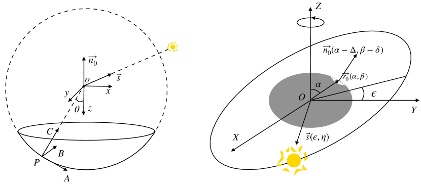
Figure 1: Three coordinate systems in this paper: Coordinate system $oxyz$ for calculating the illuminated domain in the crater, $PABC$ for calculating the effective radiative force of an arbitrary surface element, and $OXYZ$ for averaging the YORP torque over the spin and orbital motion.

However, accurately calculating the YORP effect on a real asteroid remains a challenge, as it has been demonstrated to be highly sensitive to surface topology (Statler 2009; Breiter et al. 2009), such as uniform small-scale roughness (Rozitis & Green 2012), boulders (Golubov & Krugly 2012; Golubov et al. 2014; Ševeček et al. 2015; Golubov 2017; Golubov & Scheeres 2019; Golubov et al. 2021; Golubov & Lipatova 2022), and craters (Zhou et al. 2022). Although the YORP torque caused by boulders and the tangential radiative force has been well studied, the YORP effect caused by concave structures has not yet been fully explored. More specifically, there are two kinds of concave structures on asteroid surfaces. The first one corresponds to craters, which result from impacts that an asteroid’s surface undergoes during its history and which can cover a large size range and be distributed in various ways. The second corresponds to surface roughness, which corresponds to uniformly distributed small-scale concave features that originate from the continuous effect of various processes that take place at the surface, such as thermal fatigue and space weathering. In our study, we consider both craters and surface roughness. While a pioneering study by Rozitis & Green (2012) used numerical simulations to investigate the effect of roughness, the high computational expense of such simulations prevents a comprehensive exploration of the functional dependence of this effect and its application to the global spin evolution of asteroid populations.

In addition to the precise calculation of the complete YORP effect, the long-term evolution of asteroids needs to account for stochastic collisions that affect this evolution, because each collision introduces a YORP torque due to the resulting crater. Bottke et al. (2015) performed a first study of the YORP effect accounting for craters caused by collisions, finding strong implications in the age estimate of asteroid families. However, their introduction of the concept of the stochastic YORP effect due to collisions assumed an arbitrary reset timescale for the YORP cycle. In reality, this reset timescale depends on the actual occurrence of each impact causing a crater on the asteroid’s surface and the resulting change in the YORP effect. In summary, collisions and the YORP and Yarkovsky effects are all coupled with each other in a way that is so far not well understood.

To account explicitly for the YORP torque caused by roughness and craters, Zhou et al. (2022) developed a semi-analytical model that is computationally efficient for the crater-induced YORP (CYORP) torque. The CYORP torque is defined as the torque difference between the crater and the flat ground:

$$\@vec{T}_{\rm CYORP}=\@vec{T}_{\rm crater}-\@vec{T}_{\rm ground}.$$ (1)

In general, it takes the form of the following scaling rule with the radius of the crater $R_{0}$ and of the asteroid radius $R_{\rm ast}$:

$$\@vec{T}_{\rm CYORP}=W\frac{\Phi}{c}R_{0}^{2}R_{\rm ast},$$ (2)

where $\Phi$ is the flux of solar radiation at the asteroid’s semimajor axis, and $W$ is the CYORP coefficient, which in turn depends on the obliquity and irregularity of the asteroid, and the depth-to-diameter ratio, location, thermal inertia, and albedo of the crater. As a first step, this model assumed a zero thermal conductivity. Zhou et al. (2022) found that roughness or craters that cover 10% of the asteroid’s surface area could produce a CYORP torque comparable to the normal YORP (NYORP) torque, which arises from the macroscopic shape, with ignorance of the fine surface structure. Based on this number, which assumes that all craters have a depth-to-diameter ratio of 0.16, the reset of the YORP torque by the CYORP torque could be as short as 0.4 Myr.

However, the effects of finite thermal conductivity, self-radiation, and self-scattering were not considered in Zhou et al. (2022). In the present paper, we propose a semi-analytical model that accounts for the effects of self-sheltering, self-radiation, self-scattering, and non-zero thermal conductivity. This new model allows a more general exploration of the functional dependence of the CYORP effect. Moreover, as this semi-analytical model is much more efficient than a purely numerical one, it can be used to study the combined influence of the YORP effect, collisions, and the Yarkovsky effect by incorporating the CYORP effect into the standard evolution model of asteroid families. We assume that the craters considered in this work are on a convex asteroid. It is possible to apply the model derived in this work to a moderately concave asteroid by approximating concave structures as craters, but this is beyond the scope of this paper.

In this paper, we describe our analytical model for the temperature field in a crater in Section 2. In Section 3, we introduce the numerical model that we developed to validate the analytical model. The main results are shown in Section 4 and Section 5. In Section 4, we analyse the effects of self-sheltering, self-radiation, and self-scattering of the crater, and in Section 5 we show the results of the calculation of the CYORP torque as a function of different variables. For the purpose of illustration, in Section 6 we provide an example of the analysis of CYORP considering a specific real asteroid shape and its surface roughness as well as the consequential rotational evolution. In Section 7 we summarise our main findings and draw conclusions.

2 Analytical model

2.1 Calculation of temperature distribution in a crater

2.1.1 Linearized analytical solution

The temperature $u$ for the surface and the layer beneath is governed by

$$\frac{\partial u}{\partial t}=\frac{K}{C\rho}\frac{\partial^{2}u}{\partial z^{2}},$$ (3)

with two boundary conditions,

$$K\frac{\partial u}{\partial z}\left|{}_{z=0}=F(t)-e\sigma u^{4}|_{z=0}\right.,$$ (4)

$$K\frac{\partial u}{\partial z}\left|{}_{z\to\infty}=0,\right.$$ (5)

and a periodic condition,

$$u\lvert_{t=2\pi/\omega}=u\lvert_{t=0},$$ (6)

where $t$ is the time, $z$ is the depth of the crater, $\omega$ is the angular velocity, $K$ is the thermal conductivity, $C$ is the specific heat capacity, $\rho$ is the bulk density of the asteroid, $e$ is the emissivity, and $\sigma$ is the Stefan-Boltzmann constant. In the following, we use the spin angle $\beta=\omega t$ to replace time for simplicity. The effect of the seasonal wave is marginal and is ignored in this work.

While the one-dimensional heat diffusion equation with the boundary condition of radiation has no complete analytical solution, it could be solved by linearizing the fourth power of the temperature, with the assumption that the temperature does not change significantly during a rotational period. For an arbitrary point in the hemispherical crater surface, the location of which is described by the polar angle $\theta$ and the azimuthal angle $\phi$, the solution of the temperature is the real part of the expression

$$u(\theta,\phi,\beta)=u_{0}(\theta,\phi)+\sum_{n=1}^{\infty}u_{n}(\theta,\phi){\rm e}^{in\beta},$$ (7)

with

$$u_{0}(\theta,\phi)=\left(\frac{F_{0}(\theta,\phi)}{e\sigma}\right)^{1/4},$$ (8)

$$u_{n}(\theta,\phi)=\frac{F_{n}(\theta,\phi)}{4e\sigma u_{0}(\theta,\phi)^{3}}\frac{{\rm e}^{iJ_{n}}}{\sqrt{2\Theta_{n}^{2}+2\Theta_{n}+1}},$$ (9)

where

$$l_{n}=\sqrt{\frac{n\omega}{2M}},$$ (10)

$$\Theta_{n}=\frac{Kl_{n}}{4e\sigma u_{0}^{3}},$$ (11)

$$\tan J_{n}=-\frac{\Theta_{n}}{\Theta_{n}+1},$$ (12)

with $M=K/\rho C$ .The function $F_{n}$ is the $n$th-order of the Fourier series of the absorbed radiation flux $F$, which is expressed as

$$F(\theta,\phi)=\sum_{n=0}^{\infty}F_{n}(\theta,\phi){\rm e}^{in\beta}.$$ (13)

We see that the only unknown variable is the absorbed radiation flux $F$. The absorbed radiation on a surface element contains three parts: solar radiation $E(\theta,\phi,\beta),$ radiation from the crater itself $H(\theta,\phi,\beta)$, and the scattering flux from the crater $G(\theta,\phi,\beta),$ which leads us to

$$F(\theta,\phi) =(1-A)(E(\theta,\phi)+H(\theta,\phi)+G(\theta,\phi))$$ (14)

$$=(1-A)\sum_{n=0}^{\infty}(E_{n}(\theta,\phi)+H_{n}(\theta,\phi)+G_{n}(\theta,\phi)){\rm e}^{in\beta},$$

where $E_{n}(\theta,\phi,\beta)$ and $H_{n}(\theta,\phi,\beta)$ denote the $n$th-order Fourier modes of $E(\theta,\phi,t)$ and $H(\theta,\phi,t)$, respectively. Here the albedo $A$ is assumed to be 0.1 for these three flux components for the sake of simplicity, although the albedo at the thermal-infrared wavelengths is almost zero. Following Equations (8), (9), and (14), we obtain

$$u_{0}(\theta,\phi)=\left(\frac{(1-A)(E_{0}(\theta,\phi)+H_{0}(\theta,\phi)+G_{0}(\theta,\phi))}{e\sigma}\right)^{1/4},$$ (15)

$$u_{n}(\theta,\phi)=\frac{(1-A)(E_{n}(\theta,\phi)+H_{n}(\theta,\phi)+G_{n}(\theta,\phi))}{4e\sigma u_{0}(\theta,\phi)^{3}}\frac{{\rm e}^{iJ_{n}}}{\sqrt{2\Theta_{n}^{2}+2\Theta_{n}+1}}.$$ (16)

Therefore, to solve the temperature $u(\theta,\phi,\beta)$, we need to obtain the Fourier series of $E(\theta,\phi,\beta)$, $H(\theta,\phi,\beta),$ and $G(\theta,\phi,\beta)$.

2.1.2 Coordinate systems

We use three coordinate systems to calculate the radiation and the force received by the crater, as shown in Fig 1. The coordinate system $OXYZ$ is an inertial frame used to calculate the averaged YORP torque over the spin and orbital motion. Based on the axis $OZ$, we define the coordinate system $oxyz$ fixed with the crater to calculate the instant solar flux. Finally, based on the axis $oz$, we define the coordinate system $PABC$ to calculate the self-sheltering effect of the crater. The self-sheltering effect for a point in the crater refers to the non-working moment of the photons reabsorbed by the shelter (i.e. the crater itself), which leads to the effective radiation force of the surface being tilted relative to the surface normal with a modified magnitude. This self-sheltering effect on the point $P$ depends on the geometry of the surrounding shelter. We adopt a simple sphere with a radius of $R_{1}$ to depict the crater shape.

In the coordinate system $OXYZ$, $OZ$ points along the rotation axis and $OXY$ is the equatorial plane. The axis $OY$ is chosen such that the normal vector of the orbit plane lies in the plane $OYZ$. The axis $OX$ follows the right-hand rule. There are three crucial vectors determining the CYORP torque expressed in polar coordinates in the coordinate system $OXYZ$: the crater position vector $\@vec{r}_{0}$ (denoted by $\alpha$ and $\beta$), the crater normal vector $\@vec{n}_{0}$ (described by $\alpha$, $\beta$, $\delta,$ and $\Delta$), and the solar position $\@vec{s}$ (described by$\epsilon$ and $\eta$), as shown in the right panel of Fig. 1. As the polar angle is between $0^{\circ}$ and $180^{\circ}$ by definition, we limit $0^{\circ}<\alpha<180^{\circ}$ and $0^{\circ}<\alpha-\Delta<180^{\circ}$ in our results.

The coordinate system $oxyz$ with the origin $o$ located at the sphere centre is fixed with the crater in order to simplify the calculation of the solar flux on the crater. The axis $oz$ points in the opposite direction to the surface normal vector $\@vec{n}_{0}$, which is also the symmetry axis of the spherical crater. The direction of axis $oy$ is along $\@vec{e}_{OZ}\times\@vec{e}_{oz}$ and $ox$ follows the right-hand rule. In this coordinate system, a crater with a depth of $h$ can be defined as

$$\mathcal{Z}\coloneqq\{(x,y,z)\in\mathbb{R}^{3}\lvert x^{2}+y^{2}+z^{2}=R_{1},z\geq R_{1}\cos\theta_{0}\},$$ (17)

with $\cos\theta_{0}={(R_{1}-h)}/{R_{1}}$.

The coordinate system $PABC$ with the origin $P$ at a chosen point on the crater is used to calculate the self-sheltering effect. The axis $PC$ is along the direction of $Po$, $PA$ points in the direction of $\@vec{e}_{oz}\times\@vec{e}_{PC}$, and $PB$ follows the right-hand rule. In our code, the effective force felt by the point $P$ is calculated first in the coordinate system $PABC$ for simplicity and this is then transformed to the coordinate system $oxyz$ by a rotation matrix.

2.1.3 Solar radiation $E$

In this section, we show how we derive the solar radiation received by an arbitrary point $P$ in the crater, whose coordinates in $oxyz$ system are $\@vec{r}_{P}=(\sin\theta\cos\phi,\sin\theta\sin\phi,\cos\theta).$ The unit position vector of the Sun in the coordinate system $OXYZ$ is described by

$$\@vec{s}_{OXYZ}=(\cos\eta,\cos\epsilon\sin\eta,\sin\epsilon\sin\eta),$$ (18)

where $\epsilon$ is the obliquity and $\eta$ is the angle of orbital motion. The transform matrix between the coordinate systems $oxyz$ and $OXYZ$ is set to

$$\mathcal{R}=\begin{pmatrix}\cos\alpha\cos\beta&\cos\alpha\sin\beta&-\sin\alpha\\ \sin\beta&-\cos\beta&0\\ -\cos\beta\sin\alpha&-\sin\alpha\sin\beta&-\cos\alpha\end{pmatrix}.$$ (19)

Therefore, the coordinates of the vector $\@vec{s}$ in the coordinate system $oxyz$ is

$$\@vec{s}_{oxyz}=$$ (20)

$$\begin{pmatrix}-\sin\alpha\sin\epsilon\sin\eta+\cos\alpha\cos\beta\cos\eta+\cos\alpha\sin\beta\cos\epsilon\sin\eta\\ \sin\beta\cos\eta-\cos\beta\cos\epsilon\sin\eta\\ -\sin\alpha\cos\beta\cos\eta-\sin\alpha\sin\beta\cos\epsilon\sin\eta-\cos\alpha\sin\epsilon\sin\eta\end{pmatrix}.$$

On the other hand, we can use the angle $\lambda$ and $\phi^{\prime}$ to represent $\@vec{s}_{oxyz}$:

$$\@vec{s}_{oxyz}=(\sin\lambda\cos\phi^{\prime},\sin\lambda\sin\phi^{\prime},-\cos\lambda),$$ (21)

such that

$$\cos\lambda=\sin\alpha\cos\beta\cos\eta+\sin\alpha\sin\beta\cos\epsilon\sin\eta+\cos\alpha\sin\epsilon\sin\eta,$$ (22)

and

$$\tan\phi^{\prime}=\frac{\sin\alpha\sin\epsilon\sin\eta-\cos\alpha\cos\beta\cos\eta-\cos\alpha\sin\beta\cos\epsilon\sin\eta}{\sin\beta\cos\eta+\cos\beta\cos\epsilon\sin\eta}.$$ (23)

The absorbed radiation flux is

$$E(\theta,\phi) =(1-A)\Phi H(\cos\lambda)H(w)(-\@vec{r}_{P}\cdot\@vec{s})$$ (24)

$$=(1-A)\Phi H(\cos\lambda)H(w)\cdot[m_{1}\cos(\beta-\beta_{1})+m_{2}]$$

where

$$w=\cos 2\lambda\cos\theta+\sin\theta_{0}-\sin 2\lambda\sin\theta\cos(\phi-\phi^{\prime}),$$ (25)

$$\tan\beta_{1}=$$ (26)

$$\frac{(\sin\alpha\cos\theta-\cos\alpha\sin\theta\cos\phi)\cos\epsilon\sin\eta-\sin\theta\sin\phi\cos\eta}{(\sin\alpha\cos\theta-\cos\alpha\sin\theta\cos\phi)\cos\eta+\cos\epsilon\sin\eta\sin\theta\sin\phi},$$

$$m_{1}=(\cos^{2}\eta+\cos^{2}\epsilon\sin^{2}\eta)^{1/2}$$ (27)

$$\cdot(\cos^{2}\theta\sin^{2}\alpha-\frac{\cos\phi\sin 2\alpha\sin 2\theta}{2}$$

$$+(\cos^{2}\alpha\cos^{2}\phi+\sin^{2}\phi)\sin^{2}\theta)^{1/2},$$

$$m_{2}=\cos\alpha\cos\theta\sin\epsilon\sin\eta+\cos\phi\sin\alpha\sin\epsilon\sin\eta\sin\theta.$$ (28)

Here, $H$ is the Heaviside function defined by

$$H(x)\coloneqq\left\{\begin{aligned} &1,x>0\\ &0,\rm else.\end{aligned}\right.$$ (29)

Using the substitution $\beta^{\prime}=\beta-\beta_{1}$, the absorbed radiation flux has the form

$$E(\theta,\phi)=\left\{\begin{aligned} &(1-A)\Phi(m_{1}\cos\beta^{\prime}+m_{2}),\beta^{\prime}_{\min}<\beta<\beta^{\prime}_{\max}\\ &0,\rm else.\end{aligned}\right.$$ (30)

Expanding Equation (30) in Fourier series, we obtain

$$E(\theta,\phi)=E_{0}+\frac{(1-A)\Phi}{\pi}\sum_{n=1}^{\infty}\left[C_{n}\cos(n\beta^{\prime})+S_{n}\sin(n\beta^{\prime})\right],$$ (31)

with

$$E_{0}=\frac{(1-A)\Phi}{2\pi}(m_{1}\sin\beta+m_{2}\beta)\left|{}_{\beta^{\prime}_{\min}}^{\beta^{\prime}_{\max}}\right.,$$ (32)

$$C_{n} =\int_{\beta^{\prime}}^{\beta_{\min}^{\prime}}(m_{1}\cos\beta_{\max}^{\prime}+m_{2})\cos(n\beta^{\prime}){\rm d}\beta^{\prime}$$ (33)

$$=\left\{\begin{aligned} &\left(\frac{m_{1}\sin 2\beta^{\prime}+2m_{1}\beta^{\prime}}{4}+m_{2}\sin\beta\right)\left|{}_{\beta_{\min}^{\prime}}^{\beta_{\max}^{\prime}}\right.,n=1\\ &\left(\frac{m_{1}n\cos\beta^{\prime}\sin n\beta^{\prime}-m_{1}\cos n\beta^{\prime}\sin\beta^{\prime}}{n^{2}-1}+\frac{m_{2}\sin(n\beta^{\prime})}{n}\right)\left|{}_{\beta_{\min}^{\prime}}^{\beta_{\max}^{\prime}}\right.,\\ &\qquad\qquad n>1,\end{aligned}\right.$$

and

$$S_{n} =\int_{\beta^{\prime}}^{\beta_{\min}^{\prime}}(m_{1}\cos\beta_{\max}^{\prime}+m_{2})\sin(n\beta^{\prime}){\rm d}\beta^{\prime}$$ (34)

$$=\left\{\begin{aligned} &-\left(\frac{m_{1}\cos\beta^{\prime 2}}{2}+m_{2}\cos\beta^{\prime}\right)\left|{}_{\beta_{\min}^{\prime}}^{\beta_{\max}^{\prime}}\right.,n=1\\ &\left(\frac{m_{1}n\cos\beta^{\prime}\cos n\beta^{\prime}+m_{1}\sin\beta^{\prime}\sin n\beta^{\prime}}{1-n^{2}}-\frac{m_{2}\cos n\beta^{\prime}}{n}\right)\left|{}_{\beta_{\min}^{\prime}}^{\beta_{\max}^{\prime}}\right.,\\ &\qquad\qquad n>1.\end{aligned}\right.$$

The $n$-th coefficient of the Fourier series of $E(\theta,\phi)$ is

$$E_{n}=\sqrt{C_{n}^{2}+S_{n}^{2}}\cdot{\rm e}^{i\Phi_{n}},$$ (35)

with

$$\tan\Phi_{n}=-\frac{S_{n}}{C_{n}}.$$ (36)

2.1.4 Self-heating effect

Due to the concave structure of the crater, the surface element in the crater also receives photons emitted by the crater itself, which is a process referred to as ‘self-heating’. In this section, we derive the self-radiation $H$ and the self-scattering $G$ as a function of the position in the crater.

Let us consider a surface element d$S_{1}$ receiving the radiation from another surface element d$S_{2}$. In the reference frame $oxyz$, the positions of d$S_{1}$ and d$S_{2}$ are

$$\@vec{r}_{1} =R_{1}(\sin\theta_{1}\cos\phi_{1},\sin\theta_{1}\sin\phi_{1},\cos\theta_{1}),$$ (37)

$$\@vec{r}_{2} =R_{1}(\sin\theta_{2}\cos\phi_{2},\sin\theta_{2}\sin\phi_{2},\cos\theta_{2}).$$ (38)

The displacement from d$S_{1}$ to d$S_{2}$ is

$$\@vec{r}_{1,2}=\@vec{r}_{2}-\@vec{r}_{1}.$$ (39)

The incident angle $\zeta_{1}$ and the emission angle $\zeta_{2}$ are defined as

$$\cos\zeta_{1}=-\@vec{r}_{1}\cdot\@vec{r}_{1,2}/R_{1}r_{1,2},$$ (40)

$$\cos\zeta_{2}=\@vec{r}_{2}\cdot\@vec{r}_{1,2}/R_{1}r_{1,2},$$ (41)

respectively. The radiation flux at the location of d$S_{1}$ produced by the thermal radiation of d$S_{2}$ is

$$H_{1,2}=\frac{e\sigma u_{2}^{4}}{\pi}\frac{\cos\zeta_{1}\cos\zeta_{2}}{\@vec{r}_{1,2}^{2}}dS_{2}.$$ (42)

Substituting Equations (37)-(41) into Equation (42), we obtain

$$H_{1,2} =\frac{e\sigma u_{2}^{4}}{4\pi R_{1}^{2}}dS_{2}.$$ (43)

For an arbitrary point, the radiation flux caused by the whole crater is

$$H(\theta,\phi) =\int_{\mathcal{Z}}\frac{e\sigma u(\theta^{\prime},\phi^{\prime})^{4}}{4\pi}\sin\theta^{\prime}d\theta^{\prime}d\phi^{\prime},$$ (44)

where $\mathcal{Z}$ is the crater surface, and is defined as

$$\mathcal{Z}\coloneqq\{(x,y,z)\in\mathbb{R}^{3}\lvert r=R_{1},\theta\in(0,\pi/2-\theta_{0}),\phi\in(0,2\pi)\}.$$ (45)

Similarly, we obtain the self-scattering term:

$$G(\theta,\phi)=\int_{\mathcal{Z}}\frac{AE(\theta^{\prime},\phi^{\prime})}{4\pi}\sin\theta^{\prime}d\theta^{\prime}d\phi^{\prime}.$$ (46)

Therefore, both $H(\theta,\phi)$ and $G(\theta,\phi)$ can be expressed in terms of $u(\theta,\phi)$ and $E(\theta,\phi)$. As $E(\theta,\phi)$ is derived in Sect. 2.1.3, the only unknown variable is the temperature $u(\theta,\phi)$, the solution for which is discussed in the following section.

2.2 Solution for temperature

We obtained the Fourier series of the solar radiation flux (Sect. 2.1.3) and the radiation flux produced by the crater (Sect. 2.1.4), which allows us to return to Equation (14) to solve the temperature distribution $u(\theta,\phi)$. We note that the self-radiation term $H$ contains the unknown temperature distribution that is to be solved.

The Fourier coefficients of the temperature of the crater follow

$$\sigma u_{0}^{4}(\theta,\phi)=(1-A)(E_{0}(\theta,\phi)+G_{0}(\theta,\phi)+H_{0}(\theta,\phi))$$ (47)

$$\sigma u_{n}(\theta,\phi)u_{0}^{3}(\theta,\phi)\frac{2{\sqrt{2\Theta_{n}^{2}+2\Theta_{n}+1}}}{(1-A){\rm e}^{iJ_{n}}}=E_{n}(\theta,\phi)+G_{n}(\theta,\phi)+H_{n}(\theta,\phi),$$

with

$$G_{n}(\theta,\phi)=\int_{\mathcal{Z}}\frac{AE_{n}(\theta^{\prime},\phi^{\prime})}{4\pi}\sin\theta^{\prime}d\theta^{\prime}d\phi^{\prime},$$ (48)

$$H_{0}(\theta,\phi)=\int_{\mathcal{Z}}\frac{e\sigma u_{0}(\theta^{\prime},\phi^{\prime})^{4}}{4\pi}\sin\theta^{\prime}d\theta^{\prime}d\phi^{\prime},$$

$$H_{n}(\theta,\phi)=\int_{\mathcal{Z}}\frac{e\sigma u_{0}(\theta^{\prime},\phi^{\prime})^{3}u_{n}(\theta^{\prime},\phi^{\prime})}{\pi}\sin\theta^{\prime}d\theta^{\prime}d\phi^{\prime}.$$

Here, terms $G$ and $H$ are the scattering flux and self-radiation flux, respectively.

2.2.1 Solution of a general form

Equations (47) have a general form:

$$f(\theta,\phi)=g(\theta,\phi)+C\int_{\mathcal{Z}}f(\theta^{\prime},\phi^{\prime})\sin\theta^{\prime}d\theta^{\prime}d\phi^{\prime}.$$ (49)

By setting

$$k=\int_{\mathcal{Z}}f(\theta^{\prime},\phi^{\prime})\sin\theta^{\prime}d\theta^{\prime}d\phi^{\prime},$$ (50)

we have

$$f(\theta,\phi)=g(\theta,\phi)+C\cdot k.$$ (51)

Substituting Equation (51) into Equation (50), we obtain

$$k=\int_{\mathcal{Z}}(g(\theta^{\prime},\phi^{\prime})+C\cdot k)\sin\theta^{\prime}d\theta^{\prime}d\phi^{\prime}.$$ (52)

Rearranging Equation (52), we find $k$ is

$$k=\frac{\int_{\mathcal{Z}}g(\theta^{\prime},\phi^{\prime})\sin\theta^{\prime}d\theta^{\prime}d\phi^{\prime}}{1-C\int_{\mathcal{Z}}\sin\theta^{\prime}d\theta^{\prime}d\phi^{\prime}},$$ (53)

with which $f(\theta,\phi)$ is solved out by Equation (51).

2.2.2 Solution for temperature

In the case of $u_{0}$,

$$f(\theta,\phi)=e\sigma u_{0}^{4}/(1-A),$$ (54)

$$g(\theta,\phi)=E_{0}(\theta,\phi)+G_{0}(\theta,\phi),$$ (55)

$$C=\frac{1}{4\pi},$$ (56)

and in the case of $u_{n}$,

$$f(\theta,\phi)=e\sigma u_{0}^{3}u_{n}\frac{2{\sqrt{2\Theta_{n}^{2}+2\Theta_{n}+1}}}{(1-A){\rm e}^{iJ_{n}}},$$ (57)

$$g(\theta,\phi)=E_{n}(\theta,\phi)+G_{n}(\theta,\phi),$$ (58)

$$C=\frac{{\rm e}^{iJ_{n}}}{2\pi\sqrt{2\Theta_{n}^{2}+2\Theta_{n}+1}}.$$ (59)

2.3 The CYORP torque

The CYORP torque is defined as the YORP torque difference between the crater and the flat ground:

$$T_{\rm CYORP}=T_{\rm crater}-T_{\rm ground}.$$ (60)

2.3.1 The YORP torque of the crater

The average radiative torque produced by the crater should be calculated in the inertial frame $OXYZ$:

$$\@vec{T}_{\rm crater}=\@vec{r}_{0,OXYZ}\times\@vec{f}_{OXYZ}.$$ (61)

Here, $\@vec{f}_{OXYZ}$ is the radiative force, and

$$\@vec{f}_{OXYZ}=\int_{\mathcal{W}}\frac{e\sigma T(\theta,\phi)^{4}}{c}\@vec{n}_{f}(\theta,\phi)dS,$$ (62)

where $\@vec{n}_{f}$ is the corrected force direction vector for each surface element. If there is no shelter around the surface element, $\@vec{n}_{f}$ is equal to the surface unit normal vector $\@vec{n}_{0}$. However, the surface element in a crater has a sky sheltered by other elements, resulting in the reabsorption of the emitted photons along the direction of the shelter.

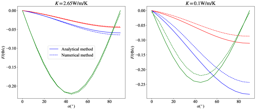
Figure 2: Radiative force of the total crater averaged over a rotational period (eight hours by default) obtained from the analytical method (solid lines) and the numerical method (dashed lines), as a function of the crater colatitude $\alpha$ for $K=2.65\rm W/m/K$ (left panel) and $K=0.1\rm W/m/K$ (right panel). The $x$, $y$, and $z$ components of the radiative force are shown in blue, red, and green, respectively. The distance of the crater here is 1 au from the Sun.

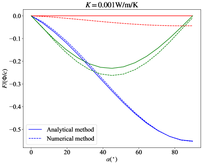
Figure 3: Same as Fig. 2 but for $K=0\rm W/m/K$ in the analytical model and $K=0.001\rm W/m/K$ in the numerical model.

For the surface element dS($\theta$, $\phi$), the radiative force is

$$\@vec{f}=-\int_{\mathcal{H}}\frac{\Phi}{\pi c}\cos\theta^{\prime}\left(\begin{aligned} &\sin\theta^{\prime}\cos\phi^{\prime}\\ &\sin\theta^{\prime}\sin\phi^{\prime}\\ &\cos\theta^{\prime}\end{aligned}\right)\sin\theta^{\prime}{\rm d}\theta^{\prime}{\rm d}\phi^{\prime}.$$ (63)

Without sheltering (e.g. for convex asteroids), $\mathcal{H}$ is replaced by the hemisphere (i.e. $\theta\in(0,\pi/2)$, $\phi\in(0,2\pi)$). In this case, the force is reduced to $2\Phi\@vec{n}_{0}/3c$.

2.3.2 The YORP torque of the flat portion of the surface

The absorbed radiation flux for a flat ground with the normal vector $\@vec{n}_{0}$ is

$$E_{\rm ground} =(1-A)\Phi H(\cos\lambda)\cos\lambda$$ (64)

$$=\left\{\begin{aligned} &(1-A)\Phi(m_{1}\cos\beta^{\prime}+m_{2}),\beta^{\prime}_{\min}<\beta^{\prime}<\beta^{\prime}_{\max}\\ &0,\rm else.\end{aligned}\right.$$

Here, $\beta^{\prime}=\beta-\beta_{1}$, with

$$\tan\beta_{1}=\frac{\sin\alpha\cos\epsilon\sin\eta}{\sin\alpha\cos\eta},$$ (65)

$$m_{1}=(\sin^{2}\alpha(\cos^{2}\eta+\cos^{2}\epsilon\sin^{2}\eta))^{1/2},$$ (66)

$$m_{2}=\cos\alpha\sin\epsilon\sin\eta,$$ (67)

and $\beta_{\rm min}$ and $\beta_{\rm max}$ are the negative and positive values of ${\rm arccos}(-m_{2}/m_{1})$, respectively.

3 Numerical model for examination

In the above analytical method, we adopted the assumption of a “small” temperature variation during a rotation period, which allows us to linearize the biquadrate of the temperature (i.e. $u^{4}\sim u_{0}^{3}\sum u_{n}{\rm e}^{\beta n{\rm i}}$). This assumption is equivalent to a high value of the thermal parameter, which is defined as

$$\Gamma=\frac{\sqrt{C\rho\omega\kappa}}{(\epsilon\sigma)^{1/4}(1-A)^{3/4}\Phi^{3/4}}.$$ (68)

In the case of a low thermal parameter, the analytical model should be used with caution. To examine the appropriate range of the thermal inertia for which our analytical model is valid, we built a one-dimensional thermophysical numerical model to perform cross-validation.

3.1 Numerical model

We used a finite difference numerical method to solve Equation 3 with the second-order Crank-Nicholson scheme:

$$c_{\rm n}u_{i,j+1,k+1}-(2c_{\rm n}+1)u_{i,j,k+1}+c_{\rm n}u_{i,j-1,k+1}$$ (69)

$$=-c_{\rm n}u_{i,j+1,k}+(2c_{\rm n}-1)u_{i,j,k}-c_{\rm n}u_{i,j-1,k}.$$

Here, $u_{i,j,k}$ represents the temperature at the depth of $(j-1)\delta z$ below the $i$-th facet at the $k$-th time step, where $i,j,$ and $k$ are integrals starting from 1 to $i_{\rm max},j_{\rm max},$ and $k_{\rm max}$. The coefficient $c_{\rm n}$ is

$$c_{\rm n}=\frac{a\delta t}{2(\delta x)^{2}}.$$ (70)

The value of $c_{\rm n}$ should be smaller than 0.5 for the convergence of the iteration.

The surface temperature is determined by the first boundary condition (Equation 4):

$$(1-A)(E_{i,k}+H_{i,k}+S_{i,k})-\sigma u_{i,1,k+1}^{4}=K\frac{u_{i,1,k+1}-u_{i,2,k}}{\delta z},$$ (71)

which can be solved by a Newtonian-Raphson iterative method. The solar flux $E_{i,k}$ on the $i$-th facet at the $k$-th time step is

$$E_{i,k}=\left\{\begin{aligned} &\Phi_{0}\@vec{n}_{i}\cdot\@vec{s}_{k}H(\@vec{n}_{i}\cdot\@vec{s}_{k}),{\rm unsheltered}\\ &0,{\rm sheltered,}\end{aligned}\right.$$ (72)

where $\Phi_{0}$ is 1364 $\rm W/m^{2}$ at the distance of 1 au to the Sun. Here, $\@vec{n}_{i}$ is the normal vector of the $i$-th facet and $\@vec{s}_{k}$ is the unit solar position vector at the $k$-th time step. Whether or not the facet is sheltered is judged according to the projections of other facets on the plane of the $i$-th facet along the solar position vector $\@vec{s}_{k}$. The self-radiation term $H_{i,k}$ is the sum of radiation from other facets:

$$H_{i,k}=\sum_{i^{\prime}\neq i}e\sigma u_{i^{\prime},1,k}^{4}\frac{-(\@vec{n}_{i}\cdot\@vec{r}_{i,i^{\prime}})(\@vec{n}_{i^{\prime}}\cdot\@vec{r}_{i,i^{\prime}})}{\pi r_{i,i^{\prime}}^{2}}S_{i^{\prime}},$$ (73)

where $\@vec{r}_{i,i^{\prime}}$ is the vector from the centre of the $i$-th facet to the centre of $i^{\prime}$-th facet, and $S_{i^{\prime}}$ is the area of the $i$-th facet. The scattering term $S_{i,k}$ is given by

$$S_{i,k}=\sum_{i^{\prime}\neq i}AE_{i^{\prime}}\frac{-(\@vec{n}_{i}\cdot\@vec{r}_{i,i^{\prime}})(\@vec{n}_{i^{\prime}}\cdot\@vec{r}_{i,i^{\prime}})}{\pi r_{i,i^{\prime}}^{2}}S_{i^{\prime}}.$$ (74)

The second boundary condition (Eq. 5) translates into

$$u_{i,j_{\rm max},k+1}=u_{i,j_{\rm max}-1,k+1}.$$ (75)

Combining Equations (69), (71), and (75), we can obtain the solution for the temperature in the next time step $u_{i,j,k+1}$ based on the temperature in the current time step $u_{i,j,k}$. We adopted an initial temperature of $u_{i,j,0}=280\leavevmode\nobreak\ \rm K$. The maximum depth is set to be a few thermal skin depths $\sqrt{K/C\rho\omega}$ and the total number of layers is set as $j_{\rm max}=50$. In order to make sure that the surface temperature is in an equilibrium state, we set the total time as $k_{\rm max}\delta t\sim 20$ spin periods. We divided the considered crater into about $1000$ facets and solve the temperature for each facet using the above method.

3.2 Comparison with the analytical model

The thermal parameters of asteroids can vary widely depending on their composition and structure. For example, the thermal conductivity of a porous material is much lower than that of a dense metal. The thermal conductivity of stony asteroids, which are made mostly of silicates, can range from about 0.1 W/mK to 1 W/mK, while the thermal conductivity of metallic asteroids is generally much higher, in the range of 20-50 W/mK. Asteroids that are composed of a mixture of rock and metal will have thermal conductivity values between those of pure rock and pure metal.

Here, we test three typical types of asteroid materials: regolith, solid basalt, and metal, whose properties are shown in Table 1. We calculate the radiative force of the total crater averaged over a rotational period (eight hours by default), as a function of the colatitude of the crater. The craters in the test are placed at 1 au from the Sun. For simplicity, we set the obliquity to $\epsilon=0$. The results computed from the analytical method and the numerical method are shown in Fig. 2. We can see that the analytical result is consistent with the numerical result to a high degree, while a large discrepancy shows up when the thermal conductivity decreases to 0.1 W/m/K. This coincides with our prerequisite of the application of our analytical method, which is that the temperature variation should be small. Therefore, our method is appropriate for solid basalt and metal materials.

Regarding regolith material, with a thermal conductivity of as low as 0.001 W/m/K, we test the model described in Zhou et al. (2022), where zero thermal conductivity is assumed. The result is shown in Fig. 3, which indicates that this latter model works well for regolith materials. Therefore, for three materials representing asteroid surfaces, our two methods, namely the one in the present work and that described in Zhou et al. (2022), behave well in modelling the YORP effect.

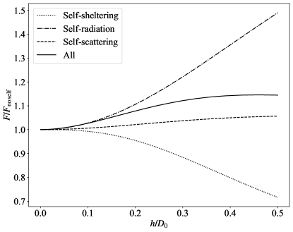
Figure 4: Ratio of the radiative force including self-modification effects to that without self-modification effects, as a function of crater depth-to-diameter ratio and accounting for different self-modification effects.

Table 1: Thermal parameter for three typical materials on asteroids, taken from Farinella et al. (1998).

	$\rho\leavevmode\nobreak\ (\rm kg/m^{3})$	$K\leavevmode\nobreak\ \rm(W/m/K)$	$C\leavevmode\nobreak\ \rm(J/kg/K)$
Regolith	1500	0.0015	680
Solid basalt	3500	2.65	680
Solid iron	8000	40	500

4 Discussion on self-modification effects

For a concave structure, there are three self-modification effects: the self-sheltering, self-radiation, and self-scattering effect. The first one refers to the radiative force modification on the surface element due to the re-absorption of photons by the crater. The second and third ones refer to the temperature increase due to the emitted photons and scattered photons from the crater itself. Previous research shows that these self-modification effects could be important for the YORP torque of the crater (Statler 2009; Rozitis & Green 2012, 2013a), but a quantitative description is still lacking. For example, it is not clear how deep the crater needs to be so that these self-modification effects can no longer be ignored. This is crucial to the validity of the commonly made assumption that the asteroid can be considered as a moderately convex shape with the craters being overlooked when evaluating the YORP torque. An essential metric in this respect is the depth-to-diameter ratio of the crater. We explore the radiative force (leading to the YORP torque) of a crater based on its depth-to-diameter ratio under varying conditions—one for each self-modification effect. Figure 4 shows our findings, situating the craters at the equator ($\alpha=\pi/2$) with a spin axis of zero-degree obliquity.

Our analysis reveals that both self-radiation and self-scattering amplify the force, raising the temperature by as much as 50% when the crater mirrors a hemisphere. In contrast, self-sheltering diminishes the force by up to 30%. Notably, the impact of self-scattering remains negligible for typical asteroid surface albedos ranging between 0.1 and 0.2. When integrating all self-modification effects, the radiative force increases by 15%.

Our result also shows that when the depth-to-diameter ratio $h/D_{0}<0.05$, the force increase is less than 1%. Therefore, for those shallow concave structures with $h/D_{0}<0.05$, no self-modification effects are needed in the YORP model for it to remain accurate. These can then be efficiently approximated as flat surfaces.

5 Analysis of the CYORP torque

As shown in a previous work (Zhou et al. 2022), the CYORP torque depends on many factors, including the depth-to-diameter ratio and location (or the colatitude $\alpha$ for example) of the crater as well as the obliquity and thermal parameter of the asteroid. In this section, we discuss the dependence of the CYORP torque on these factors. In the following, except for in Sect. 5.1, we assume the depth-to-diameter ratio to be $\sim 0.16$.

5.1 Depth-to-diameter ratio

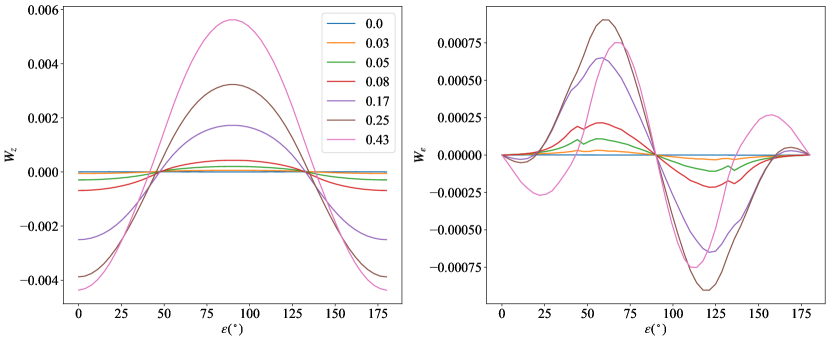
Figure 5: Spin component (left panel) and the obliquity component (right panel) of the CYORP coefficient as a function of the asteroid obliquity $\epsilon$, accounting for different depth-to-diameter ratios, which are denoted by different colours.

Asteroid craters exhibit a range of distinct features in size and shape, with diameters ranging from a few centimetres to several kilometres for large asteroids. These craters generally display bowl-shaped structures, containing central peaks and terraced walls when produced in the gravity regime. To simplify the modelling, a semi-sphere approximation is often used to represent the shape of craters.

According to the definition of CYORP torque, if the depth-to-diameter ratio reaches zero, the CYORP torque is zero (Eq. 60). Figure 5 shows the CYORP torques generated by craters with various depth-to-diameter ratios. The parameters $\delta=\Delta=\pi/6$, $K=2.65\leavevmode\nobreak\ \rm W/m/K$, and $\alpha=\pi/2$ are used. Higher depth-to-diameter ratios correspond to larger spin components of the CYORP torque. A crater with $h/D_{0}<0.05$ produces an insignificant CYORP torque, which may be disregarded. Furthermore, the depth-to-diameter ratio also impacts the obliquity component, influencing both the torque magnitude and shape of the torque curve. For instance, when the depth-to-diameter ratio is low, the asymptotic obliquity is $90^{\circ}$, while for higher depth-to-diameter ratios, new asymptotic obliquities arise around $0^{\circ}$ and $180^{\circ}$.

5.2 Crater latitude $\alpha$ and asteroid obliquity $\epsilon$

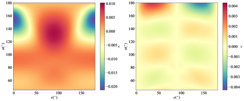
Figure 6: Spin component (left panel) and the obliquity component (right panel) of the CYORP coefficient as a function of the asteroid obliquity $\epsilon$ and the crater colatitude $\alpha(>\Delta)$, for $K=2.65\rm W/m/K$. Here, $d/D_{0}=0.16$ and $\delta=\Delta=\pi/4$.

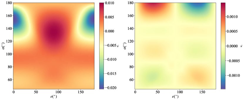
Figure 7: Same as Fig. 6 but for $K=40\rm W/m/K$.

Figure 6 displays the CYORP torque components as a function of the crater latitude and asteroid obliquity. The values of the parameters $\delta$ and $\Delta$ are set to a representative value of $\pi/4$. The spin component $W_{z}$ exhibits symmetry about the axis $\epsilon=90^{\circ}$, while the obliquity component $W_{\epsilon}$ is anti-symmetric. The minimum and maximum values of the torque occur when the obliquity is $0\circ$ or $90^{\circ}$, with the absolute value of these extrema reaching up to 0.02. The coefficient of the obliquity component of the CYORP torque is considerably smaller, with a maximum value of 0.004.

For comparison, the typical value of the normal YORP spin coefficient is 0.005 for type I/II and $<0.001$ for type III/IV asteroids . The ratio of the CYORP torque to the normal YORP torque scales as

$$\frac{T_{\rm CYORP}}{T_{\rm NYORP}}=\frac{W_{\rm CYORP}S_{\rm crater}}{W_{\rm YORP}S_{\rm asteroid}}.$$ (76)

Setting the ratio to 1, we find that the total area of concave structures needs to be as large as 1/4 and 1/20 of the asteroid surface area for type I/II and type III/IV asteroids, respectively.

5.3 Thermal parameter

When the asteroid rotates quickly and has high heat conductivity, a higher value of the thermal parameter arises, resulting in a smaller variation in temperature. To explore the role of the thermal parameter, we employ the same parameters as in Sect. 5.2, but with $K=40\leavevmode\nobreak\ \rm W/m/K$ for metal materials, and the resulting CYORP torques are depicted in Fig. 7. The comparison with Fig. 6 reveals that the spin component remains relatively unchanged, while the obliquity component displays significant variation. This observation aligns with the prior assertion that the thermal parameter mainly impacts the obliquity component (Vokrouhlickỳ & Čapek 2002). In the regime of high thermal conductivity, the obliquity component diminishes as the thermal conductivity increases.

Figure 8: Spin component (left panel) and the obliquity component (right panel) of the CYORP coefficient as a function of $\Delta(<\alpha)$ and $\delta$, for $K=2.65\rm W/m/K$. Here, $d/D_{0}=0.16$ and $\alpha=\epsilon=\pi/6$.

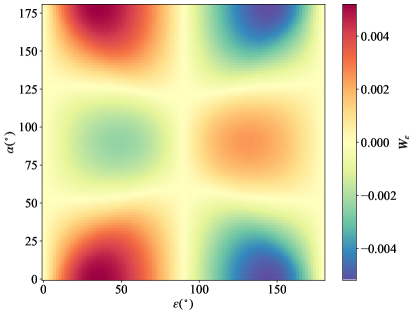
Figure 9: Obliquity component (right panel) of the CYORP coefficient as a function of the asteroid obliquity $\epsilon$ and the crater colatitude $\alpha$ for $K=2.65\rm W/m/K$. Here, $d/D_{0}=0.16$ and $\delta=\Delta=0$.

5.4 Irregularity $\delta$ and $\Delta$

The angular parameters $\delta$ and $\Delta$ are used to describe the irregularity of the asteroid, where $\delta=0$ and $\Delta=0$ correspond to a perfect sphere. We explore the CYORP torque as a function of $\delta$ and $\Delta$ with fixed asteroid obliquity and crater colatitude of $\pi/4$. The results are presented in Fig. 8. We can see that for the spin component, $\delta$ controls the torque magnitude while $\Delta$ controls the torque direction.

Zhou et al. (2022) demonstrates that the CYORP torque vanishes for $\delta=0$. However, in the presence of finite thermal inertia, the obliquity component of the CYORP torque arises while the spin component remains negligible. Figure 9 illustrates the variation of the CYORP obliquity component with the asteroid obliquity and the crater colatitude when $\delta$ and $\Delta$ are both zero. The CYORP torque has a tendency to lead the asteroid obliquity to $90\circ$ when the crater is near the poles, while it leads to an asymptotic obliquity of $0^{\circ}$ or $180^{\circ}$ when the crater is near the equator.

6 Application of the CYORP effect on a real asteroid

6.1 Roughness

The surface roughness of asteroids is produced by several processes, including micrometeorite impacts, thermal fatigue, ejecta, or outgassing. It was found that the YORP torque is extremely sensitive to the small-scale surface structures (Statler 2009; Breiter et al. 2009). The microscopic beaming effect of regolith grain-size-scale roughness (¡1 mm) was shown —using the Hapke reflectance and emissivity model (Breiter & Vokrouhlickỳ 2011)— to have a marginal influence on the YORP effect. The transverse heat conduction across thermal skin depth ($\sim 1\leavevmode\nobreak\$cm) causes an asymmetric thermal emission of the east and west sides of a boulder, giving rise to a systematic positive YORP torque (Golubov & Krugly 2012; Golubov & Lipatova 2022). The importance of the various self-modification effects of a concave feature on the surface was considered gradually and numerical approaches were taken to study it (Statler 2009; Rozitis & Green 2012, 2013a). It was found that the concave feature of surface roughness could dampen the YORP torque by tens of percent. While the pioneering studies by Rozitis & Green (2012) shed light on the effects of roughness, the computational expense and difficulty in studying the functional dependence means that there are severe limitations to the numerical method. In contrast, the analytical method that we introduce in the present study, and its computational efficiency, simplify the application of roughness-induced YORP effects to real asteroids or binary systems. Given the objective of our semi-analytical method to provide a rapid assessment of the impact of surface roughness, it is particularly well-suited for models of asteroids with rough convex shapes derived from light-curve observations. However, when dealing with high-resolution shape models, especially those that possess a resolution of a few centimetres (the scale of the thermal skin), a 3D thermal model becomes essential for accurate calculations, owing to the presence of the tangential YORP (TYORP) effect, which accounts for the transverse heat conduction inside a boulder.

For illustrative purposes, to demonstrate the application of our method, we randomly selected the main belt asteroid (272) Antonia as an example. This choice is representative of the majority of asteroids lacking detailed information obtained through in situ observations. We used the shape model obtained from Hanuš et al. (2013). To optimise the performance of our model, we assume a relatively high thermal conductivity of 1 W/m K. We uniformly distributed the roughness across the asteroid’s surface and investigated the total YORP torque (NYORP + CYORP). To do so, we input the normal vector and position vector of surface elements in the shape model to our CYORP model to obtain the CYORP torque coefficient of each surface element. We then used the area of each surface element to calculate the CYORP torque and sum up all CYORP torques generated by all surface elements. The depth-to-diameter is assumed to be 0.5, following the assumption made by Rozitis & Green (2012). This has been compared with the sole NYORP torque. The result is depicted in Fig. 10. Our findings confirm that the roughness-induced CYORP torque damps the normal YORP torque. Specifically, for the asteroid (272) Antonia, the spin component of the torque experiences a damping effect of approximately 35%, while the obliquity component is damped by approximately 64%.

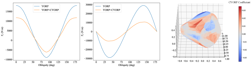
Figure 10: YORP torque damped by the CYORP effect in the case of asteroid (272) Antonia. The spin component and the obliquity component are shown in the left and middle panels, respectively. The right panel shows the CYORP coefficient distribution over the asteroid’s surface.

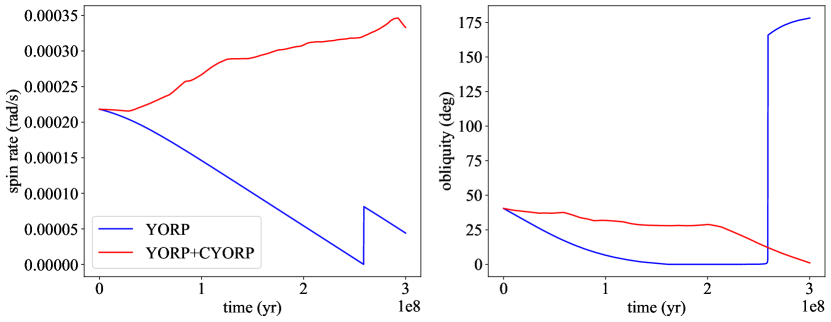
Figure 11: Evolution of the spin rate (left panel) and the obliquity (right panel) of a 10 km synthetic asteroid. In the presence of the static YORP torque (blue line), the asteroid gradually decelerates until it reaches a quasi-non-rotational state. Subsequently, we impose a new rotational state on the asteroid by assigning random values of rotational speed and obliquity. Conversely, when incorporating the CYORP torque (red line), the asteroid follows a different path, exhibiting random fluctuations in its spin rate due to the occurrence of impacts, creating new craters that lead to changes in the CYORP torque. As a result, the asteroid experiences intermittent transitions between spin up and spin down.

6.2 Rotational evolution

The rotational dynamics of asteroids are primarily governed by two key processes: collisions and the YORP effect. The timescale for reorientation of the spin axis resulting from angular momentum transfer during a collision can be expressed as (Farinella et al. 1998)

$$\tau_{\rm imp,re-ori}=746\left({R_{\rm ast}\over 1{\rm km}}\right)^{4/3}\left({\omega\over 3\times 10^{-4}{\rm s^{-1}}}\right)^{5/6}\rm Myr.$$ (77)

On the other hand, the typical timescale associated with the YORP effect is approximately given by:

$$\tau_{\rm YORP}\sim 4\left({R_{\rm ast}\over 1{\rm km}}\right)^{2}\left({\omega\over 3\times 10^{-4}{\rm s^{-1}}}\right)\rm Myr.$$ (78)

Clearly, the YORP timescale is shorter than $\tau_{\rm imp,re-ori}$, although its specific value exhibits considerable variation across different asteroids. Consequently, it is widely accepted that the YORP effect primarily governs the rotational evolution of small objects, while collisions play a dominant role in larger objects. The classic static YORP model —which assumes an invariable YORP torque until the asteroid spins up to disruption or spins down to a quasi-static rotation— has been used to study the long-term rotational evolution of asteroids (Rubincam 2000; Pravec et al. 2005; Bottke et al. 2015).

A more intricate model, referred to as the ‘stochastic YORP model’ (Bottke et al. 2015), takes into account the resetting of the YORP torque caused by collisions, which arises from the high sensitivity of the YORP effect to surface morphology. Although a suggested timescale of 1 Myr has been proposed for YORP reset (Bottke et al. 2015), a quantitative assessment of the torque changes resulting from craters is yet to be explored. The CYORP effect offers a powerful tool for investigating the stochastic YORP effect. While a comprehensive examination of the stochastic YORP effect is beyond the scope of this paper, we present an example of integrating the CYORP effect into the static YORP model.

In our simulation, a random YORP coefficient is assigned within the range of -0.005 to 0.005, with the coefficient’s sign matching that of the torque. The CYORP torque is introduced specifically when a collision event takes place. The timescale for the impact by an asteroid with the size $R_{\rm imp}$ is

$$\tau_{{\rm imp}}=\frac{1}{P_{\rm i}\pi R_{\rm Antonia}^{2}\Delta N(R>R_{\rm imp})},$$ (79)

where

$$N(R>R_{\rm imp})=C_{R}\left(\frac{R_{\rm imp}}{1\leavevmode\nobreak\ {\rm km}}\right)^{-b_{R}}.$$ (80)

Here, $P_{\rm i}=2.85\times 10^{-18}\rm km^{-2}yr^{-1}$ is the intrinsic collision probability, $C_{R}=6\times 10^{5}$, and $b_{R}=2.2$ (Holsapple 2022). In the strength regime formulation, the crater produced by an impactor with the size of $R_{\rm imp}$ has a size of

$$R_{\rm crater}=1.306R_{\rm imp}\left({\rho_{\rm imp}\over\rho_{\rm ast}}^{0.4}\right)\left({Y\over\rho v_{\rm imp}}\right)^{-0.205},$$ (81)

with $Y=100$ Pa and $v_{\rm imp}=5.3$ km/s. In the gravity regime,

$$R_{\rm crater}=0.59\left({\rho_{\rm ast}\over m_{\rm imp}}\right)^{-1/3}\left({\rho_{\rm ast}\over\rho_{\rm imp}}\right)^{0.00138}\left({g_{\rm ast}R_{\rm ast}\over v_{\rm imp}}\right)^{-0.17},$$ (82)

where $g_{\rm ast}$ is the surface gravity of the asteroid. In each time step ($\sim 10^{3}$ years), we calculate the numbers of impact craters of different sizes, according to Eq. 79 and Eq. 81. We then assign each crater with a random surface element of the polyhedron model of the asteroid Antonia, after which we can calculate the CYORP torque. Finally, we add the CYORP torque to the normal YORP torque directly calculated from the shape model in order to obtain the total YORP torque. The spin rate evolves following

$$\dot{\omega}={T_{z}\over I},$$ (83)

with $I$ being the maximum moment of inertia and $T_{z}$ being the torque component that is along a spin vector. The obliquity evolves according to

$$\dot{\epsilon}={T_{\epsilon}\over I\omega},$$ (84)

where $T_{\epsilon}$ is the torque component that changes the obliquity.

There exist two possible end states in a YORP cycle: either the asteroid’s rotation slows down until it reaches a quasi-non-rotational state, or it accelerates to the spin threshold for shape change or disruption with a period of approximately 2.2 hours. Upon completing a YORP cycle, the asteroid’s rotational state is updated by assigning a new random rotational speed and obliquity. The impact of introducing CYORP torques can be observed in the evolution of a 10 km asteroid, as depicted in Fig. 11. Notably, significant differences arise when considering the inclusion of CYORP torques.

Nonetheless, the rotational evolution of asteroids currently lacks a standardised model. Some models propose that after spinning down to a non-rotational state, the asteroid’s spin rate is assigned a new random value within a specified range (Hanuš et al. 2011; Bottke et al. 2015), while some assume it continues to spin up under the YORP effect (Pravec et al. 2008; Marzari et al. 2020). By selecting an initial spin rate for a new rotational state, Holsapple (2022) reproduces the spin evolution without the YORP effect. Hence, rather than attempting to address the entire complexity of the problem, our objective in this study is to present an illustrative example of the interaction between CYORP and the conventional YORP effect. Furthermore, we underscore the significance of the CYORP effect in the long-term rotational evolution of asteroids. A comprehensive investigation of the rotational evolution of asteroid groups is left for future research.

7 Summary and conclusions

The YORP effect is a thermal torque produced by radiation from the irregular surface of the asteroid. It has been demonstrated that this effect is highly sensitive to surface topology (Statler 2009; Breiter et al. 2009), including small-scale roughness (Rozitis & Green 2012), boulders (Golubov & Krugly 2012), and craters (Zhou et al. 2022). In this study, we developed a semi-analytical model for calculating the temperature field of a crater, which accounts for the effects of self-sheltering, self-radiation, self-scattering, and non-zero thermal conductivity. Using this model, we investigated the crater-induced YORP (CYORP) effect in a computationally efficient manner (about three orders of magnitude faster than the numerical method), allowing for a comprehensive exploration of the functional dependence of the CYORP effect and its incorporation into the rotational and orbital evolution of asteroids. The main results and conclusions of this study can be summarised as follows.

Our semi-analytical model for the CYORP effect is valid in the high-thermal-conductivity regime ($K>0.1\rm W/m/K$). This suggests that the model is suitable for application to materials such as solid basalt and metal, which are usually beneath the regolith on asteroid surfaces but may be exposed to sunlight due to the formation of deep craters.

The CYORP effect is significant when the crater depth-to-diameter ratio is greater than 0.05. The self-modification effects of a concave structure, including the self-sheltering effect, self-radiation effect, and self-scattering effect, are stronger with a higher depth-to-diameter ratio. For concave structures with a depth-to-diameter ratio of smaller than 0.05, the surface can be treated as a convex shape without introducing significant inaccuracies. The typical value of the CYORP coefficient for the spin component is 0.01, which is insensitive to the thermal parameter, while the obliquity component decreases from 0.004 for basalt to 0.001 for metal. For a z-axis symmetric shape (e.g. a spinning top shape), the spin component of the CYORP torque vanishes while the obliquity component survives, which implies that the spin acceleration of such symmetric shapes does not change significantly under the effect of crater formation.

Using our semi-analytical method, we confirm that the YORP torque can be damped by the surface roughness, which was first discovered by Rozitis & Green (2012). The fast computation of our semi-analytical model allows us to consider more flexible configurations of surface roughness, such as a space-varying roughness distribution, roughness on components of binary asteroids, and so on.

The magnitude and directional change of the YORP coefficient at each impact are assessed for the first time using our CYORP model. While a complete investigation of the spin evolution of asteroids is left for future work, we show that rotational evolution can be severely affected by collisions.