Causal Contextual Bandits with Adaptive Context

Abstract

We study a variant of causal contextual bandits where the context is chosen based on an initial intervention chosen by the learner. At the beginning of each round, the learner selects an initial action, depending on which a stochastic context is revealed by the environment. Following this, the learner then selects a final action and receives a reward. Given $T$ rounds of interactions with the environment, the objective of the learner is to learn a policy (of selecting the initial and the final action) with maximum expected reward. In this paper we study the specific situation where every action corresponds to intervening on a node in some known causal graph. We extend prior work from the deterministic context setting to obtain simple regret minimization guarantees. This is achieved through an instance-dependent causal parameter, $\lambda$, which characterizes our upper bound. Furthermore, we prove that our simple regret is essentially tight for a large class of instances. A key feature of our work is that we use convex optimization to address the bandit exploration problem. We also conduct experiments to validate our theoretical results, and release our code at the project GitHub Repository.

1 Introduction

Recent years have seen an active interest in causal bandits from the research community (Lattimore et al., 2016; Sen et al., 2017a; b; Lee & Bareinboim, 2018; Yabe et al., 2018; Lee & Bareinboim, 2019; Lu et al., 2020; Nair et al., 2021; Lu et al., 2021; 2022; Maiti et al., 2022; Varici et al., 2022; Subramanian & Ravindran, 2022; Xiong & Chen, 2023). In this setting, one assumes an environment comprising of causal variables that are random variables that influence each other as per a given causal (directed, and acyclic) graph. Specifically, the edges in the causal DAG represent causal relationships between variables in the environment. If one of these variables is designated as a reward variable, then the goal of a learner then is to maximize their reward by intervening on certain variables (i.e., by fixing the values of certain variables). The rest of the variables, that are not intervened upon, take values as per their conditional distributions, given their parents in the causal graph. In this work, as is common in literature, we assume that the variables take values in $\{0,1\}$. Of particular interest are causal settings wherein the learner is allowed to perform atomic interventions. Here, at most one causal variable can be set to a particular value, while other variables take values in accordance with their underlying distributions.

It is relevant to note that when a learner performs an intervention in a causal graph, they get to observe the values of multiple other variables in the causal graph. Hence, the collective dependence of the reward on the variables is observed through each intervention. That is, from such an observation, the learner may be able to make inferences about the (expected) reward under other values for the causal variables (Peters et al., 2017). In essence, with a single intervention, the learner is allowed to intervene on a variable (in the causal graph), allowed to observe all other variables, and further, is privy to the effects of such an intervention. Indeed, such an observation in a causal graph is richer than a usual sample from a stochastic process. Hence, a standard goal in causal bandits is to understand the power and limitations of interventions. This goal manifests in the form of developing algorithms that identify intervention(s) that lead to high rewards, while using as few observations/interventions as possible. We use the term intervention complexity (rather than sample complexity) for our algorithm, to emphasize that interventions are richer than samples.

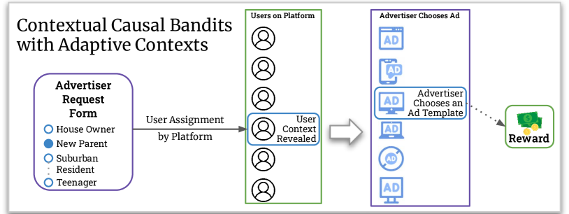
Figure 1: Flowchart illustrating the decision-making process of an advertiser posting ads on a platform like Amazon, and the subsequent interaction with the platform.

In the learning literature, there are several objectives that an algorithm designer might consider. Cumulative regret, simple regret, and average regret have prominently been studied in literature (Lattimore & Szepesvári, 2020; Slivkins et al., 2019). In this work we focus on minimizing simple regret, wherein the algorithm is given a time budget, up to which it may explore, at which time it has to output a near-optimal policy.

Addressing causal bandits, the notable work of Lattimore et al. (2016) obtains an intervention-complexity bound for minimizing simple regret with a focus on atomic interventions and parallel causal graphs. Maiti et al. (2022) extend this work to obtain intervention-complexity bounds for simple regret in causal graphs with unobserved variables. The work by Lu et al. (2022) extends this setting to causal Markov decision processes (MDPs), while addressing the cumulative regret objective. Combinatorial causal bandits have been studied by Feng & Chen (2023) and Xiong & Chen (2023).

Causal contextual bandits have been studied by Subramanian & Ravindran (2022) where the contexts may be chosen by the learner (rather than be provided by the environment). Here we generalize Subramanian & Ravindran (2022) to a setting where the context is provided by the environment, adaptively, in response to an initial choice of the learner.

Motivating Example: Consider an advertiser looking to post ads on a web-page, say Amazon. They may make requests for a certain type of user demographic to Amazon. Based on this initial request, the platform may actually choose one particular user to show the ad to. At this time, certain details about the user are revealed to the advertiser. For example, the platform may reveal some of the user demographics, as well as certain details about their device. Based on these details, the advertiser may choose one particular ad to show the user. In case the user clicks the ad, the advertiser receives a reward. The goal of the learner is to find optimal choices for initial user preference, as well as ad-content such that user clicks are maximized. We illustrate this example through Figure 1 where we indicate the choices available for template and content interventions.

1.1 Our Contributions

We develop an algorithm to identify near-optimal interventions in causal bandits with adaptive context, and show that the simple regret of such an algorithm is indeed tight for several instances. We highlight the main contributions of our work below.

1. We develop and analyze an algorithm for minimizing simple regret for causal bandits with adaptive context in an intervention efficient manner. We provide an upper-bound on intervention complexity in Theorem 1.

2. Interestingly, the intervention complexity of our algorithm depends on an instance dependent structural parameter—referred to as $\lambda$ (see equation (3))— which may be much lower than $nk$, where $n$ is the number of interventions and $k$ is the number of contexts.

3. Notably, our algorithm uses a convex program to identify optimal interventions. Unlike prior work that uses optimization to design exploration (for example see Yabe et al. (2018)), we show (in Appendix Section E) that the optimization problem we design is convex, and is thus computationally efficient. Using convex optimization to design efficient exploration is in fact a distinguishing feature of our work.

4. We provide lower bound guarantees showing that our regret guarantee is tight (up to a log factor) for a large family of instances (see Section 4 and Appendix Section F).

5. We demonstrate using experiments (see Section 5) that our algorithm performs exceeding well as compared to other baselines. We note that this is because $\lambda\ll nk$ for $n$ causal variables and $k$ contexts.

In conclusion, we provide a novel convex-optimization based algorithm for Causal MDP exploration. We analyze the algorithm to come up with an instance dependent parameter $\lambda$. Further, we prove that our algorithm is sample efficient (see Theorems 1 and 2).

1.2 Additional Related Work

Description	Reference
Simple regret for bandits with parallel causal graphs	Lattimore et al. (2016)
Simple regret for atomic soft interventions	Sen et al. (2017a)
Simple regret for non-atomic interventions in causal bandits	Yabe et al. (2018)
Cumulative regret for general causal graphs	Lu et al. (2020)
Simple regret in the presence of unobserved confounders	Maiti et al. (2022)
Cumulative regret for unknown causal graph structure	Lu et al. (2021)
Cumulative regret for causal contextual bandits with latent confounders	Sen et al. (2017b)
Simple and cumulative regret for budgeted causal bandits	Nair et al. (2021)
Cumulative regret for Linear SEMs	Varici et al. (2022)
Cumulative regret for combinatorial causal bandits	Feng & Chen (2023)
Cumulative regret for Causal MDPs	Lu et al. (2022)
Best-intervention for combinatorial causal bandits	Xiong & Chen (2023)
Additive Causal Bandits with Unknown Graph	Malek et al. (2023)
Structural Causal Bandits with Unobserved Confounders	Wei et al. (2024)
Confounded Budgeted Causal Bandits	Jamshidi et al. (2024)
Cumulative Regret for Causal Bandits with Lipschitz SEMs	Yan et al. (2024)
Simple regret for causal contextual bandits	Subramanian & Ravindran (2022)
Simple regret for causal contextual bandits with adaptive context	Our work

Table 1: Summary of prior work in causal bandits

Ever since the introduction of the causal bandit framework by Lattimore et al. (2016), we have seen multiple works address causal bandits in various degrees of generality and using different modelling assumptions. Sen et al. (2017a) addressed the issue of soft atomic interventions using an importance sampling based approach. Soft interventions in the linear structural equation model (SEM) setting was addressed recently by Varici et al. (2022). Yabe et al. (2018) proposed an optimization based approach for non-atomic interventions. This work was extended by Xiong & Chen (2023) to provide instance dependent regret bounds. They also provide guarantees for binary generalized linear models (BGLMs). The question of unknown causal graph structure was addressed by Lu et al. (2021), whereas Nair et al. (2021) study the case where interventions are more expensive than observations.

Maiti et al. (2022) addressed simple regret for graphs containing hidden confounding causal variables, while cumulative regret in general causal graphs was addressed by Lu et al. (2020). A notable work by Lu et al. (2022) formulates the framework for causal MDPs, and they provide cumulative regret guarantees in this setting. Causal contextual bandits were addressed by Subramanian & Ravindran (2022); Sen et al. (2017b), and we extend these works to adaptive contexts.

We summarize the main works in this thread in Table 1 and provide a more detailed set of related works in Appendix A.

2 Notations and Preliminaries

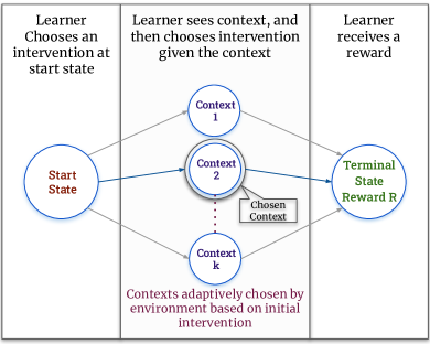
((a)) Illustrative figure for causal contextual bandit with adaptive context.

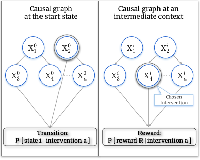
((b)) Illustrative Figure for Causal Graph at start state and at some intermediate context $i\in[k]$.

Figure 2: The transition to a particular context (chosen context in the figure on the left) is decided by the environment, whereas the interventions at the start state and an intermediate context (chosen interventions in the figure on the right) are chosen by the learner.

We model the causal contextual bandit with adaptive context as a contextual bandit problem with a causal graph corresponding to each context. The actions at each context are given by interventions on the causal graph. Additionally, we have a causal graph at the start state, and the context is stochastically dependent on the intervention on the causal graph at the start state. For ease of notation, we will call the start state of the learner as context $0$. The agent starts at context $0$, chooses an intervention, then transitions to one of $k$ contexts $[k]=\{1,\dots,k\}$, chooses another intervention, and then receives a reward; see Figure 2(a).

Assumptions on the Causal Graph: Formally, let $\mathcal{C}$ be the set of contexts $\{0,1,\dots,k\}$. Then, at each context, there is a Causal Bayesian Network (CBN) represented by a causal graph; see Figure 2(b). In particular, at each context $i\in\mathcal{C}$, the causal graph is composed of $n$ variables $\{X^{i}_{1},\dots,X^{i}_{n}\}$. Each $X^{i}_{j}$ takes values from $\{0,1\}$, with an associated conditional probability (of being equal to 0 or 1), given the other variables in the causal graph. We make the following mild assumptions on the causal graph at each context.

1. The distribution of any node $X_{i}$ conditioned on it’s parents in the causal graph is a Bernoulli random variable with a fixed parameter.

2. The causal graph at each context is semi-Markovian. This is equivalent to making the following assumptions on the graph. No hidden variable in the graph has a parent. Further, every hidden variable has at most two children, both observable.

3. We transform the causal graph for each context as follows: For every hidden variable with two children, we introduce bidirected edges between them. If no path of bidirected edges exists between an intervenable node and its child, the graph is identifiable – a necessary and sufficient condition for estimating the graph’s associated distribution.(Tian & Pearl, 2002).

Table 2: Summary of notations for our paper

Notation	Explanation
Context $0$	Start state
Context $[k]$	Intermediate contexts $\{1,\dots,k\}$
$X^{i}_{j}$	Causal Variables: $X^{i}_{j}\in\{0,1\}\enspace\text{ for all }i\in[k],\enspace j\in[n]$
$do(\cdot)$	An atomic intervention of the form $do()$, $do(X_{j}^{i}=0)$ or $do(X_{j}^{i}=1)$
$\mathcal{A}_{i}$	Set of atomic interventions at context $i$
$N$	$N:=|\mathcal{A}_{i}|=2n+1\enspace\text{ for all }i\in[k]$
$R_{i}$	Reward on transition from context $i$
$m_{i}$	Causal observational threshold at context $i\in\{0,\dots,k\}$
$M$	diagonal matrix of $m_{i}$ values
$P\in\mathbb{R}^{N\times k}$	Transition probabilities matrix: $\left[P_{(a,i)}=\mathbb{P}\{i\enspace\mid\enspace a\}\right]_{a\in\mathcal{A}_{0},i\in[k]}$
$p_{+}$	Transition threshold $p_{+}=\min\{P_{(a,i)}\mid P_{(a,i)}>0\}$
$\pi:\mathcal{C}\to\mathcal{A}$	Policy, a map from contexts to interventions.
i.e. $\pi(i)\in\mathcal{A}_{i}$ for $i\in\{0\}\cup[k]$
$\mathbb{E}\left[R_{i}\mid\pi(i)\right]$	Expectation of the reward at context $i$ given intervention $\pi(i)$

Interventions: Furthermore, we are allowed atomic interventions, i.e., we can select at most one variable and set it to either $0$ or $1$. We will use $\mathcal{A}_{i}$ to denote the set of atomic interventions available at context $i\in\{0,\ldots,k\}$; in particular, $\mathcal{A}_{i}=\left\{do()\right\}\cup\left\{do(X^{i}_{j}=0),do(X^{i}_{j}=1)\right\}$ for $\ j\in[n]$. We note that $do()$ is an empty intervention that allows all the variables to take values from their underlying conditional distributions. Also, $do(X^{i}_{j}=0)$ and $do(X^{i}_{j}=1)$ set the value of variable $X^{i}_{j}$ to $0$ and $1$, respectively, while leaving all the other variables to independently draw values from their respective distributions. Note that for all $i\in[k]$, we have $\lvert\mathcal{A}_{i}\rvert=2n+1$. Write $N:=2n+1$.

Reward: The environment provides the learner with a $\{0,1\}$ reward upon choosing an intervention at context $i\in[k]$, which we denote as $R_{i}$. Note that $R_{i}$ is a stochastic function of variables $X^{i}_{1},\dots,X^{i}_{n}$. In particular, for all $j\in[n]$ and each realization $X^{i}_{j}=x_{j}\in\{0,1\}$, the reward $R_{i}$ is distributed as $\mathbb{P}\{R_{i}=1\mid X^{i}_{1}=x_{1},\ldots$ $,X^{i}_{n}=x_{n}\}$.

Given such conditional probabilities, we will write $\mathbb{E}[R_{i}\mid a]$ to denote the expected value of reward $R_{i}$ when intervention $a\in\mathcal{A}_{i}$ is performed at context $i\in[k]$. Here the expectation is over the parents of the variable $R_{i}$ in the causal graph, with the intervened variable set at the required value. Note that these parents (of $R_{i}$) may in turn have conditional distributions given their parents. The leaf nodes of the causal graph are considered to have unconditional Bernoulli distributions. For instance, $\mathbb{E}[R_{i}\mid do(X^{i}_{j}=1)]$ is the expected reward when variable $X^{i}_{j}$ is set to $1$, and all the other variables independently draw values from their respective (conditional) distributions. Indeed, the goal of this work is to develop an algorithm that maximizes the expected reward at context $0$.

Causal Observational Threshold: We denote by $m_{i}$, the causal observational threshold from Maiti et al. (2022) at context $i$. This is computed as follows. Let $\widehat{q}_{j}^{i}=\min_{\text{Parents}(X_{j}^{i}),x\in\{0,1\}}\mathbb{P}\{X_{j}^{i}=x\mid\text{Parents}(X_{j}^{i})\}$. Further, let $S^{i}_{\tau}=\{\widehat{q}_{j}^{i}:(\widehat{q}_{j}^{i})^{c}<1/\tau\}$ be sets parameterized by $\tau$ for every $\tau\in[2,2n]$, where $c$ indicates the c-component size. Then $m_{i}=\min\{\tau\text{ such that }|S^{i}_{\tau}|\leq\tau\}$. The existence of such a threshold at each context is guaranteed by the assumptions we made on the CBNs. In addition, let $\smash{M\in\mathbb{N}^{k\times k}}$ denote the diagonal matrix of $m_{1},\ldots,m_{k}$.

Transitions at Context 0: At context $0$, the transition to the intermediate contexts $[k]$ stochastically depends on the random variables $\{X^{0}_{1},\dots,X^{0}_{n}\}$. Here, $\mathbb{P}\{i\enspace\mid\enspace a\}$ denotes the probability of transitioning into context $i\in[k]$ with atomic intervention $a\in\mathcal{A}_{0}$; recall that $\mathcal{A}_{0}$ includes the do-nothing intervention. We will collectively denote these transition probabilities as matrix $P:=\left[P_{(a,i)}=\mathbb{P}\{i\enspace\mid\enspace a\}\right]_{a\in\mathcal{A}_{0},i\in[k]}$. Furthermore, write the transition threshold $p_{+}$ to denote the minimum non-zero value in $P$. Note that matrix $P\in\mathbb{R}^{\lvert\mathcal{A}_{0}\rvert\times k}$ is fixed, but unknown.

Policy: A map $\pi:\{0,\dots,k\}\to\mathcal{A}$, between contexts and interventions (performed by the algorithm), will be referred to as a policy. Specifically, $\pi(i)\in\mathcal{A}_{i}$ is the intervention at context $i\in\{0,1,\ldots,k\}$. Note that, for any policy ${\pi}$, the expected reward, which we denote as $\mu(\pi)$, is equal to $\sum_{i=1}^{k}\mathbb{E}\left[R_{i}\ \mid\ {\pi}(i)\right]\cdot\mathbb{P}\{i\ \mid\ \pi(0)\}$. Maximizing expected reward, at each intermediate context $i\in[k]$, we obtain the overall optimal policy $\pi^{*}$ as follows. For $i\in[k]$:

$$\pi^{*}(i) =\operatorname*{arg\,max}_{a\in\mathcal{A}_{i}}\ \mathbb{E}\left[R_{i}\mid a\right]\vspace{-0.05in}$$ (1)

$$\vspace{-0.05in}\pi^{*}(0) =\operatorname*{arg\,max}_{b\in\mathcal{A}_{0}}(\sum_{i=1}^{k}\ \mathbb{E}\left[R_{i}\mid\pi^{*}(i)\right]\cdot\mathbb{P}\{i\mid b\})$$ (2)

Our goal then is to find a policy $\pi$ with (expected) reward as close to that of $\pi^{*}$ as possible.

Simple Regret: Conforming to the standard simple-regret framework, the algorithm is given a time budget $T$, i.e., the learner can go through the following process $T$ times — (a) start at context $0$. (b) Choose an intervention $a\in\mathcal{A}_{0}$. (c) Transition to context $i\in[k]$. (d) Choose an intervention $a\in\mathcal{A}_{i}$. (e) Receive reward $R_{i}$. At the end of these $T$ steps, the goal of the learner is to compute a policy. Let the policy returned by the learner be $\widehat{\pi}$. Then the simple regret is defined as the expected value: $\mathbb{E}[\mu(\pi^{*})-\mu(\widehat{\pi}]$. Our algorithm seeks to minimize such a simple regret.

3 Main Algorithm and its Analysis

We now provide the details relating to our main Algorithm, viz. ConvExplore.

Algorithm 1 ConvExplore: Convex Exploration Algorithm

1:Input: Total rounds $T$

2:Estimate the transition probabilities $\widehat{P}$ from the start state to the intermediate contexts for time $T/3$, by performing interventions at context 0 in a round robin manner.

3:Estimate the causal observational threshold matrix $\hat{M}$ for time $T/3$, by performing interventions at context 0 as per frequency vector $\tilde{f}$ where $\tilde{f}\leftarrow\operatorname*{arg\,max}\limits_{\text{fq.~{}vector }f}\enspace\min\limits_{\text{contexts [k]}}\widehat{P}^{\top}f$.

4:Estimate the reward matrix $\widehat{\mathcal{R}}$ for time $T/3$, by performing interventions at context 0 as per frequency vector $\widehat{f}^{*}$ where $\widehat{f}^{*}\leftarrow\operatorname*{arg\,min}\limits_{\text{fq.~{}vector }f}\,\max\limits_{\text{interventions }\mathcal{I}_{0}}\widehat{P}\hat{M}^{1/2}\left(\widehat{P}^{\top}f\right)^{\circ-\frac{1}{2}}$.

5:Estimate the optimal action at each intermediate context $\widehat{\pi}(i)\enspace\forall i\in[k]$ based on $\widehat{\mathcal{R}}$. Let the estimate of optimal reward be $\widehat{\mathcal{R}}(\widehat{\pi}(i))$.

6:Estimate the optimal action at the start context $\widehat{\pi}(0)$, based on the transition probabilities $\widehat{P}$ and the optimal reward estimates $\widehat{\mathcal{R}}(\widehat{\pi}(i))$.

7:return $\widehat{\pi}=\{\widehat{\pi}(0),\widehat{\pi}(1),\dots,\widehat{\pi}(k)\}$ .

The algorithm can be described by five main steps. In the first step, we estimate the transitions to intermediate contexts. In the second step, we estimate the causal observational thresholds at these contexts. In the third step, we estimate the rewards upon doing interventions at these contexts. With good reward estimates and transition probability estimates, the computation of a good policy at the intermediate contexts (step 4) and at the start state (step 5) is straightforward. This Algorithm relies on three subroutines which are detailed in Section B of the Appendix. The key aspect of this algorithm is in designing the exploration of interventions (at the start state and at the intermediate contexts) to be regret-optimal – i.e. trading off exploration time between different interventions such that the policy eventually obtained has near-optimal reward.

Our algorithm (ConvExplore) uses subroutines to estimate the transition probabilities, the causal parameters, and the rewards. From these, it outputs the best available interventions as its policy $\widehat{\pi}$. Given time budget $T$, the algorithm uses the first $T/3$ rounds to estimate the transition probabilities (i.e., the matrix $P$) in Algorithm 2. The subsequent $T/3$ rounds are utilized in Algorithm 3 to estimate causal parameters $m_{i}$s. Finally, the remaining budget is used in Algorithm 4 to estimate the intervention-dependent reward $R_{i}$s, for all intermediate contexts $i\in[k]$.

To judiciously explore the interventions at context $0$, ConvExplore computes frequency vectors $f\in\mathbb{R}^{\lvert\mathcal{A}_{0}\rvert}$. In such vectors, the $a$th component $f_{a}\geq 0$ denotes the fraction of time that each intervention $a\in\mathcal{A}_{0}$ is performed by the algorithm, i.e., given time budget $T^{\prime}$, the intervention $a$ will be performed $f_{a}T^{\prime}$ times. Note that, by definition, $\sum_{a}f_{a}=1$ and the frequency vectors are computed by solving convex programs over the estimates. The algorithm and its subroutines throughout consider empirical estimates, i.e., find the estimates by direct counting. Here, let $\widehat{P}$ denote the computed estimate of the matrix $P$ and $\smash{\hat{M}}$ be the estimate of the diagonal matrix $M$. We obtain a regret upper bound via an optimal frequency vector $\widehat{f}^{*}$ (see Step 4 in ConvExplore).

Recall that for any vector $x$ (with non-negative components), the Hadamard exponentiation ${\circ-0.5}$ leads to the vector $y=x^{\circ-0.5}$ wherein $y_{i}=1/\sqrt{x_{i}}$ for each component $i$. We next define a key parameter $\lambda$ that specifies the regret bound in Theorem 1 (below). At a high-level, parameter $\lambda$ captures the “exploration efficacy” in the MDP, that takes into account the transition probabilities $P$ and the exploration requirements $M$ at the intermediate layer. Identification of this parameter is a relevant technical contribution of our work; see Section C.1 for a detailed derivation of $\lambda$.

$$\lambda:=\min_{\text{fq.~{}vector}f}\ \left\lVert PM^{0.5}\left(P^{\top}f\right)^{\circ-0.5}\right\rVert_{\infty}^{2}$$ (3)

Furthermore, we will write $f^{*}$ to denote the optimal frequency vector in equation (3). Hence, with vector $\nu:=P{M}^{0.5}(P^{\top}f^{*})^{\circ-0.5}$, we have $\lambda=\max_{a}\nu_{a}^{2}$. Note that Step 4 in ConvExplore addresses an analogous optimization problem, albeit with the estimates $\smash{\widehat{P}}$ and $\hat{M}$. Also, we show in Lemma 11 (see Section E in the supplementary material) that this optimization problem is convex and, hence, Step 4 admits an efficient implementation.

To understand the behaviour of $\lambda$, we first note that whenever the $m_{i}$ values at the contexts $i\in[k]$ are low, the $\lambda$ value is low. Specifically, the $m_{i}$ values can go as low as $2$ (when the $q^{i}_{j}$s are all $\frac{1}{2}$), removing the dependence of $\lambda$ on $n$. The upper-bound on $\lambda$ is $nk$. We see this by first upper-bounding each $m_{i}$ by $n$. Then, note that whenever $\max_{a\in\mathcal{A}}P\{i|a\}\geq 1/k$, then $\exists f$ such that $P^{\top}f=u$ where $u=\{\frac{1}{k},\dots,\frac{1}{k}\}$. Now we can compute that $||P\cdot u^{\circ-0.5}||^{2}_{\infty}=k$, and thereby $\lambda<nk$; See footnote.

The following theorem that upper bounds the regret of ConvExplore is the main result of the current work. The result requires the algorithm’s time budget to be at least $T_{0}:=\widetilde{O}\left(N\max(m_{i})/p_{+}^{3}\right)$

Theorem 1.

Given number of rounds $T\geq T_{0}$ and $\lambda$ as in equation (3), ConvExplore achieves regret

$${\rm Regret}_{T}\in\mathcal{O}\left(\sqrt{\max\left\{\frac{\lambda}{T},\frac{m_{0}}{Tp_{+}}\right\}\log\left(NT\right)}\right)$$

Observe that $m_{0}/Tp_{+}$ is independent of the number of contexts and interventions. Therefore $\lambda$ dominates when number of interventions at an intermediate context is large.

4 Analysis of the Lower Bound

Since ConvExplore solves an optimization problem, it is a priori unclear that a better algorithm may not provide a regret guarantee better than Theorem 1. In this section, we show that for a large class of instances, it is indeed the case that the regret guarantee we provide is optimal. We provide a lower bound on regret for a family of instances. For any number of contexts $k$, we show that there exist transition matrices $P$ and reward distributions ($\mathbb{E}[R_{i}\mid a]$) such that regret achieved by ConvExplore  (Theorem 1) is tight, up to log factors.

Theorem 2.

For any $q^{i}_{j}$ corresponding to causal variables at contexts $i\in[k]$, there exists a transition matrix $P$, and probabilities $q^{0}_{j}$ corresponding to causal variables $\{X^{0}_{j}\}_{j\in[n]}$, and reward distributions, such that the simple regret achieved by any algorithm is

$${\rm Regret}_{T}\in\Omega\left(\sqrt{\frac{\lambda}{T}}\right)$$

We provide the details of the proof of Theorem 2 in Section F in the supplementary material.

5 Experiments

We first list a few baseline algorithms that we compare ConvExplore with. This is followed by a complete description of our experimental setup. Finally, we present and discuss our main results.

Uniform Exploration: This algorithm uniformly explores the interventions in the instance. It first performs all the atomic interventions $a\in\mathcal{A}_{0}$ at the start state $0$ in a round robin manner. On transitioning to any context $i\in[k]$, it performs atomic interventions $b\in\mathcal{A}_{i}$ in a round robin manner. UnifExplore achieves a regret upperbounded by $\tilde{\mathcal{O}}(\sqrt{nk/T})$, which is also the optimal lower bound for non-causal algorithms. Hence it serves as a good comparison as it achieves an optimal non-causal simple regret. We plot the comparison with this non-causal regret optimal exploration in Figure 3. We plot the regret with respect to (A) the number of rounds of exploration and (B) with the $\lambda$ values of our instance. Notice that at extremely high $\lambda$ values ConvExplore does not perform well, as such an instance does not particularly benefit from the causal structure. Even so, with further tuning of constants in our Algorithm, we should achieve a performance similar to UnifExplore.

Figure 3: We plot the Simple Regret under ConvExplore and UnifExplore. The figure on the left (3a) plots expected simple regret vs time, for the setup $n=25$, $k=25$, $\lambda=50$, $\varepsilon=0.3$ and $m=2$ for all contexts. The figure on the right (3b) plots expected simple regret with $\lambda$. It was performed with the parameters: $T=25000$, $k=25$, $m_{0}=2$ and $\varepsilon=0.3$.

Other Baselines: We now consider several other baselines for comparison, that have been used in literature. Primary amongst these are: (1) UCB at the start state, as well as the intermediate contexts (2) Thompson sampling at the start state, as well as the intermediate contexts (3) Round-robin at the start state, and UCB at the intermediate contexts (4) Round-robin at the start state, and Thomson sampling at the intermediate contexts and (5) UnifExplore which is round-robin at both the start state and at the intermediate contexts.

Setup: We consider $k=25$ intermediate contexts and a causal graphs with $n=25$ variables ($2n+1=51$ interventions) at each context. The rewards are distributed Bernoulli($0.5+\varepsilon$) for intervention $X^{1}_{1}=1$ and Bernoulli($0.5$) otherwise where $\varepsilon=0.3$ in the experiments. We set $m_{i}=m\enspace\forall i\in[k]$. As in experiments in prior work, we set $q^{i}_{j}=0$ for $j\leq m_{i}$ and $0.5$ otherwise. Let $k=n$ here. At state $0$, on taking action $a=do()$, we transition uniformly to one of the intermediate contexts. On taking action $do(X^{0}_{i}=1)$, we transition with probability $2/k$ to context $i$ and probability $1/k-1/(k(k-1))$ to any of the other $k-1$ contexts.

We perform two experiments in this setting. In the first one, we run ConvExplore and UnifExplore for time horizon $T\in\{1000,\dots,25000\}$. In the second experiment, we run ConvExplore and UnifExplore for a fixed time horizon $T=25000$ with $\lambda$ varying in the set $\{50,75,\dots,625\}$. To vary $\lambda$, we vary $m_{i}$ for the intermediate contexts in the set $\{2,3,\ldots,25\}$. We average the regret over $10000$ runs for each setting. We use CVXPY (Diamond & Boyd (2016)) to solve the convex program at Step 4 in ConvExplore. We release our code in entirety in our anonymized GitHub project repository, for the community to use and improve.

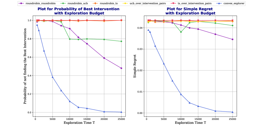
Figure 4: We plot various baselines for two metrics of interest (1) Probability of the algorithm finding the best interventions and (2) Simple regret. These plots illustrate how these metrics vary with the exploration budget.

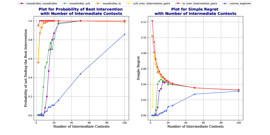
Figure 5: We plot the variation of probability of finding the best intervention and simple regret with the number of contexts. Notice the outperformance of ConvExplore vs. the other baselines.

Results of comparison with UnifExplore: In Figure 3a, we compare the expected simple regret of ConvExplore vs. UnifExplore. Our plots indicate that ConvExplore outperforms UnifExplore and its regret falls rapidly as $T$ increases. In Figure 3b, we plot the expected simple regret against $\lambda$ for ConvExplore and UnifExplore that was obtained in Experiment $2$, and empirically validate their relationship that was proved in Theorem 1.

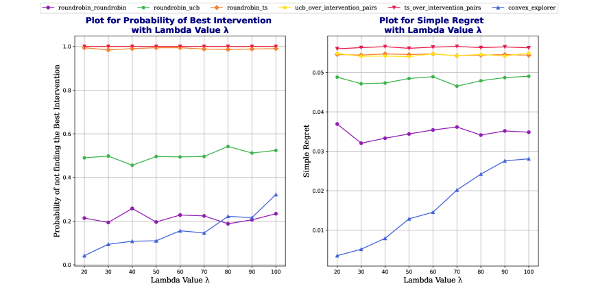
Figure 6: We plot the variation of probability of finding the best intervention and simple regret with $\lambda$ value. Notice that ConvExplore is the only algorithm that is causal-aware and hence varying with $\lambda$.

Results of comparison withother baselines: We find that ConvExplore significantly outperforms baselines other than UnifExplore. Specifically Thompson samplling and UCB are not well tuned to the exploration problem, and hence perform poorly in both the metrics of (1) simple regret as well as (2) probability of finding the best intervention. A mixture of round-robin at the start state with these alternatives at the intermediate context also perform poorly with respect to ConvExplore for this particular exploration problem. In Figure 4 we plot the metrics with exploration budget. In Figure 5 we plot the metrics of interest with the number of contexts at the intermediate stage. Finally, in Figure 6, we plot the simple regret as well as probability of finding the best intervention with our parameter $\lambda$, while keeping the number of intermediate contexts the same. The results of these experiments and full details can be found here.

6 Conclusions

We studied extensions of the causal contextual bandits framework to include adaptive context choice. This is an important problem in practice and the solutions therein have immediate practical applications. The setting of stochastic transition to a context accounted for non-trivial extensions from Subramanian & Ravindran (2022) who studied targeted interventions. We developed a Convex Exploration algorithm for minimizing simple regret under this setting. Furthermore, while Maiti et al. (2022) studied the simple causal bandit setting with unobserved confounders, our work addresses causal contextual bandits with adaptive contexts, under the same constraint of allowing unobserved confounders (assuming identifiability). We identified an instance dependent parameter $\lambda$, and proved that the regret of this algorithm is $\tilde{\mathcal{O}}(\sqrt{\frac{1}{T}\max\{\lambda,\frac{m_{0}}{p_{+}}\}})$. The current work also established that, for certain families of instances, this upper bound is essentially tight. Finally, we showed through experiments that our algorithm performs better than uniform exploration in a range of settings. We believe our method of converting the exploration in the causal contextual bandit setting is novel, and may have implications outside the causal setting as well.

Possible generalizations of this work include extensions to non-binary reward settings. Another natural extension would be to derive bounds for L-layered MDPs, extending from the adaptive contextual bandit setting we consider. It would be interesting to see whether that problem reduces to convex exploration as well. Finally, extending convex exploration methods from this paper to other more general simple regret problems may also be a promising avenue for future research.

7 Acknowledgements

Siddharth Barman gratefully acknowledges the support of the Walmart Center for Tech Excellence (CSR WMGT-23-0001) and a SERB Core research grant (CRG/2021/006165).

Appendix A Related Work

In our work, we draw from prior literature from causality as well as from multi-armed bandits. We will briefly cover these two in the following section.

A.1 Multi-armed bandits:

The stochastic Multi-Armed Bandit (MAB) setup is a standard model for studying the exploration-exploitation trade-off in sequential decision making problems (Kuleshov & Precup, 2014; Bubeck et al., 2012). Such trade-offs arise in several modern applications, such as ad placement, website optimization, recommendation systems, and packet routing (Bouneffouf et al., 2020) and are thus a central part of the theory relating to online learning (Slivkins et al., 2019; Lattimore & Szepesvári, 2020).

Traditional performance measures for MAB algorithms have focused on cumulative regret (Auer et al., 2002; Agrawal & Goyal, 2012; Auer & Ortner, 2010), as well as best-arm identification under the fixed confidence (Even-Dar et al., 2006) and fixed budget (Audibert et al., 2010) settings. In some settings however, one may be interested in optimizing the exploration phase. Another variant of regret that has been considered is the mini-max regret (Azar et al., 2017) which focuses on the worst case over all possible environments. However, as a metric for pure exploration in MABs, simple regret has been proposed as a natural performance criterion (Bubeck et al., 2009). In this setting, we allow for some period of exploration, after which the learner has to choose an arm. The simple regret is then evaluated as the difference between the average reward of the best arm and the average reward of the learner’s recommendation. We focus on simple regret in this work.

Each of these performance metrics come with their own lower bounds (Orabona et al., 2012; Osband & Van Roy, 2016; Bubeck et al., 2012), which are naturally the benchmarks for any algorithms proposed. The lower bound on simple regret is known to be $\mathcal{O}(\sqrt{n/T})$ for a stochastic multi-armed bandit problem with $n$ arms. This bound is obtained from the lower bound for pure exploration provided by Mannor & Tsitsiklis (2004).

Note that, a naive approach to the causal bandit problem which simply treats an intervention on each of exponentially many combinations of the nodes as an arm, may thus incur an exponential regret. We now review some of the literature from Causality, which helps in addressing the causal aspects of the problem.

A.2 Causality:

There are three broad threads in causality related to our work. These are causal graph learning, causal testing and causal bandits. We address relevant works in these areas below.

Learning Causal Graphs: Tian & Pearl (2002) laid the grounds for analysing functional functional constraints among the distributions of observed variables in a causal Bayesian networks. Similarly, Kang & Tian (2006) derive such functional constraints over interventional distributions. These two seminal works lead to a great interest in the problem of learning causal graphs.

There have been several studies that provide algorithms to recover the causal graphs from the conditional independence relations in observational data (Pearl & Verma, 1995; Spirtes et al., 2000; Ali et al., 2005; Zhang, 2008). Subsequent work considered the setting when both observational and interventional data are available (Eberhardt et al., 2005; Hauser & Bühlmann, 2014). Kocaoglu et al. (2017a) extend the causal graph learning problem to a budgeted setting. Shanmugam et al. (2015) uses interventions on sets of small size to learn the causal structure. Kocaoglu et al. (2017b) provide an efficient randomized algorithm to learn a causal graph with confounding variables.

Testing over Bayesian networks: Given sample access to an unknown Bayesian Network (Canonne et al., 2017), or Ising model (Daskalakis et al., 2019), one may wish to decide whether an unknown model is equal to a known fixed model, and analyse the sample complexity of this hypothesis test. Acharya et al. (2018) address this question by introducing the concept of covering interventions. These covering interventions allow us to understand the behaviour of multiple interventions (that are covered) simultaneously. We utilize the concept of covering interventions from Acharya et al. (2018) towards our question of finding the optimal intervention in a causal bandit. The area of reinforcement learning over causal bandits has also been studied in Zhang (2020).

Apart from these areas in causality, our primary problem of causal bandits have been addressed by Lattimore et al. (2016); Maiti et al. (2022); Sen et al. (2017a); Lu et al. (2020); Nair et al. (2021); Sen et al. (2017b); Lu et al. (2021; 2022); Varici et al. (2022); Xiong & Chen (2023). We detail these in the main Related Works Section 1.2.

Appendix B Algorithms in Detail

In this section, we outline the three algorithms that are used as helpers in ConvExplore. The first that we outline now, Algorithm 2, would be used to estimate the transition probabilities out of context $0$ on taking various actions.

Algorithm 2 Estimate Transition Probabilities

1:Input: Time budget $T^{\prime}$

2:For time $t\leftarrow\{1,\dots,\frac{T^{\prime}}{2}\}$ do

3:  Perform $do()$ at context $0$. Transition to $i\in[k]$

4:  Count number of times context $i\in[k]$ is observed

5:  Update $\widehat{q}_{j}^{0}=\mathbb{P}\left\{X_{j}^{0}=1\right\}$

6:end

7:Using $\widehat{q}_{j}^{0}$s, estimate $m_{0}$ and the set $\mathcal{A}_{m_{o}}$. Estimate $\widehat{P}_{(a,i)}=\mathbb{P}[i\mid a]$ $\enspace\forall a\in\mathcal{A}_{m_{0}}^{c}$ and $i\in[k]$

8:For intervention $a\in\mathcal{A}_{m_{o}}$ at context $0$

9:  For time $t\leftarrow\{1,\dots\frac{T^{\prime}}{2\lvert\mathcal{A}_{m_{0}}\rvert}\}$

10:    Perform $a\in\mathcal{A}_{m_{o}}$ and transition to some $i\in[k]$

11:    Count number of times context $i$ is observed

12:  end

13:end

14:Estimate $\widehat{P}_{(a,i)}=\mathbb{P}[i\mid a]$ for each $a\in\mathcal{A}_{m_{0}}$ and contexts $i\in[k]$

15:return Estimated matrix $\widehat{P}=\left[\widehat{P}_{(a,i)}\right]_{i\in[k],a\in\mathcal{A}_{0}}$

Next we estimate the causal parameters at all contexts $i\in[k]$ through Algorithm 3. Then we will use Algorithm 4 to estimate the rewards on various interventions at the intermediate contexts.

For estimating the causal parameters, we use a variant of SRM-ALG from Maiti et al. (2022), which estimates the causal observational threshold $m_{i}$, under the setting of unobserved confounders and identifiability. We note that even in the presence of general causal graphs with hidden variables, SRM-ALG is able to efficiently estimate the rewards of all the arms simultaneously using the observational arm pulls. As mentioned in Section 3 of Maiti et al. (2022), the challenge is to identify the optimal number of arms with bad estimates during the initial phase of the algorithm, such that these arms can be intervened upon at the later phase. The $q_{i}(x)$ parameter is the minimum conditional probability of $X=x$, given different configurations of the parents of $X$. Once we have these estimates, the remaining algorithm can proceed as per usual.

Algorithm 3 Estimate Causal Parameters

1:Input: Frequency vector $\tilde{f}$ and time budget $T^{\prime}$

2:Update $f(a)\leftarrow\frac{1}{2}\left(\tilde{f}(a)+\frac{1}{\lvert\mathcal{A}_{0}\rvert}\right)\enspace\forall a\in\mathcal{A}_{0}$

3:For intervention $a\in\mathcal{A}_{0}$

4:  For time $t\leftarrow\{1,\dots T^{\prime}\cdot f(a)\}$

5:    Perform $a\in\mathcal{A}_{0}$ and transition to some $i\in[k]$.

6:    At context $i$, perform $do()$ and observe $X^{i}_{j}$s

7:    Update $\widehat{q}_{j}^{i}=\min_{\text{Parents}(X_{j}^{i}),x\in\{0,1\}}\mathbb{P}\left\{X_{j}^{i}=x\mid\text{Parents}(X_{j}^{i})\right\}$

8:  end

9:end

10:Using $\widehat{q}_{j}^{i}$s, estimate $\widehat{m}_{i}$ values for each context $i\in[k]$

11:return $\hat{M}$, the diagonal matrix of the $\widehat{m}_{i}$ values

Note that in Algorithm 4 there are two phases. In the first phase, we carry out estimates for interventions that have high probability of being observed on the $do()$ intervention. In the second phase, we specifically perform interventions which have not been observed often enough. This is similar to Algorithm 2 where we carry out the two phases of interventions at context $0$.

Algorithm 4 Estimate Rewards

1:Input: Optimal frequency $f^{*}$, min-max frequency $\tilde{f}$, and time budget $T^{\prime}$

2:Set $f(a)\leftarrow\frac{1}{3}\left(f^{*}(a)+\tilde{f}(a)+\frac{1}{\lvert\mathcal{A}_{0}\rvert}\right)\enspace\forall a\in\mathcal{A}_{0}$

3:For intervention $a\in\mathcal{A}_{0}$ at context $0$

4:  For time $t\leftarrow\{1,\dots f(a)\cdot T^{\prime}/2\}$

5:    Perform $a\in\mathcal{A}_{0}$. Transition to some $i\in[k]$. Perform $do()$ at context $i\in[k]$.

6:    Observe variables $X^{i}_{j}$’s and rewards $R_{i}$.

7:  end

8:end

9:Find the set $\mathcal{A}_{m_{i}}\enspace\forall i\in[k]$ using $q^{i}_{j}$ estimates.

10:Estimate mean reward $\widehat{\mathcal{R}}_{(b,i)}=\mathbb{E}\left[R_{i}\mid b\right]$ for each $b\in\mathcal{A}_{m_{i}}^{c}$

11:For intervention $a\in\mathcal{A}_{0}$ at context $0$

12:  For time $t\leftarrow\{1,\dots f(a)\cdot T^{\prime}/2\}$

13:    Perform $a\in\mathcal{A}_{0}$ and transition to some $i\in[k]$.

14:    Iteratively perform $b\in\mathcal{A}_{m_{i}}$. Observe $R_{i}$

15:  end

16:end

17:Estimate mean reward $\widehat{\mathcal{R}}_{(b,i)}=\mathbb{E}\left[R_{i}\mid b\right]$ for each $b\in\mathcal{A}_{m_{i}}$

18:return $\widehat{\mathcal{R}}=\left[\widehat{\mathcal{R}}_{(b,i)}\right]_{i\in[k],b\in\mathcal{A}_{i}}$

Appendix C Proof of Theorem 1

In this section, we restate Theorem 1 and provide its proof, along with all the lemmas that are used in the proof.

Theorem.

Given number of rounds $T\geq T_{0}$ and $\lambda$ as in equation (3), ConvExplore achieves regret

$${\rm Regret}_{T}\in\mathcal{O}\left(\sqrt{\max\left\{\frac{\lambda}{T},\frac{m_{0}}{Tp_{+}}\right\}\log\left(NT\right)}\right)$$

C.1 Proof of Theorem 1

To prove the theorem, we analyze the algorithm’s execution as falling under either good event or bad event, and tackle the regret under each.

Definition 1.

We define five events, $E_{1}$ to $E_{5}$ (see Table 3), the intersection of which we call as good event, $E$, i.e., $\textit{good event }E:=\bigcap_{i\in[5]}E_{i}$. Furthermore, we define the $\textit{bad event }F:=E^{c}$.

Table 3: Table enumerating Good Events

Event	Condition	Explanation
$E_{1}$	$\sum\limits_{i=1}^{k}\lvert\widehat{P}_{(a,i)}-P_{(a,i)}\rvert\leq\frac{p_{+}}{3}\forall a\in\mathcal{A}_{0}$	for every intervention $a\in\mathcal{A}_{0}$, the empirical estimate of transition probability in each of Algorithms 2, 3 and 4 is good, up to an absolute factor of $p_{+}/3$
$E_{2}$	$\widehat{m}_{0}\in[\frac{2}{3}m_{0},2m_{0}]$	our estimate for causal parameter $m_{0}$ for state 0 is relatively good in Algorithm 2.
$E_{3}$	$\widehat{m}_{i}\in[\frac{2}{3}m_{i},2m_{i}]\quad\forall i\in[k]$	our estimate for causal parameter $m_{i}$ for each context $i\in[k]$ is relatively good in Algorithm 3.
$E_{4}$	$\sum_{i\in[k]}\lvert\widehat{P}_{(a,i)}-P_{(a,i)}\rvert\leq\zeta$, $\forall a\in\mathcal{A}_{0}$	The error in estimated transition probability in Algorithm 2 sums to less than $\zeta$ where $\zeta:=\sqrt{\frac{150m_{0}}{Tp_{+}}\log\left(\frac{3T}{k}\right)}$
$E_{5}$	$\left\lvert\mathbb{E}\left[R_{i}\mid a\right]-\widehat{\mathcal{R}}_{(a,i)}\right\rvert\leq\widehat{\eta}_{i}\enspace\forall i\in[k],a\in\mathcal{A}_{i}$	The error in reward estimates in Algorithm 4 is bounded by $\widehat{\eta}_{i}$ where $\widehat{\eta}_{i}=\sqrt{\frac{27\widehat{m}_{i}}{T(\widehat{P}^{\top}\widehat{f}^{*})_{i}}\log\left(2TN\right)}$

Considering the estimates $\widehat{P}$ and $\hat{M}$, along with frequency vector $\widehat{f}^{*}$ (computed in Step 4), we define random variable

$$\widehat{\smash{\lambda}}:=\left\lVert\widehat{P}\hat{M}^{1/2}\left(\widehat{P}^{\top}\widehat{f}^{*}\right)^{\circ-\frac{1}{2}}\right\rVert_{\infty}^{2}.$$

Note that $\widehat{\smash{\lambda}}$ is a surrogate for $\lambda$. We will show that under the good event, $\widehat{\smash{\lambda}}$ is close to $\lambda$ (Lemma 3).

Recall that ${\rm Regret}_{T}:=\mathbb{E}[\varepsilon(\pi)]$ and here the expectation is with respect to the policy ${\pi}$ computed by the algorithm. We can further consider the expected sub-optimality of the algorithm and the quality of the estimates (in particular, $\widehat{P}$, $\hat{M}$ and $\widehat{\smash{\lambda}}$) under good event (E).

Based on the estimates returned at Step 4 of ConvExplore, either the good event holds, or we have the bad event. We obtain the regret guarantee by first bounding sub-optimality of policies computed under the good event, and then bound the probability of the bad event.

Lemma 1.

For the optimal policy $\pi^{*}$, under the good event ($E$), we have $\sum_{i\in[k]}P_{(\pi^{*}(0),i)}\mathbb{E}\left[R_{i}\ \mid\ \pi^{*}(i)\right]-\sum\widehat{{P}}_{(\pi^{*}(0),i)}\widehat{\mathcal{R}}_{(\pi^{*}(i),i)}\leq\mathcal{O}\left(\sqrt{\max\{\widehat{\smash{\lambda}},m_{0}/p_{+}\}/T\log\left(NT\right)}\right)$

Proof.

We add and subtract $\sum_{i\in[k]}P_{(\pi^{*}(0),i)}\mathcal{\widehat{R}}_{(\pi^{*}(i),i)}$ and reduce the expression on the left to: $\sum_{i\in[k]}P_{(\pi^{*}(0),i)}(\mathbb{E}\left[R_{i}\mid\pi^{*}(i)\right]-\widehat{\mathcal{R}}_{(\pi^{*}(i),i)})+\sum_{i\in[k]}\widehat{\mathcal{R}}_{(\pi^{*}(i),i)}(P_{(\pi^{*}(0),i)}-\widehat{P}_{(\pi^{*}(0),i)})$.

We have: (a) $\widehat{\mathcal{R}}_{(\pi^{*}(i),i)}\leq 1$ (as rewards are bounded) (b) $\sum_{i\in[k]}\lvert\widehat{P}_{(\pi^{*}(0),i)}-P_{(\pi^{*}(0),i)}\rvert\leq\zeta$ (by $E_{4}$) and (c) $\left\lvert\mathbb{E}\left[R_{i}\mid\pi^{*}(i)\right]-\widehat{\mathcal{R}}_{(\pi^{*}(i),i)}\right\rvert\leq\widehat{\eta}_{i}$ (by $E_{5}$). The above expression is thus bounded above by $\sum_{i\in[k]}P_{(\pi^{*}(0),i)}\widehat{\eta}_{i}+\zeta$ Furthermore, it follows from $E_{1}$ (See Corollary 2 in Section D.1 in the supplementary material) that (component-wise) $P\leq\frac{3}{2}\widehat{P}$. Hence, the above-mentioned expression is bounded above by $\frac{3}{2}\sum_{i\in[k]}\widehat{P}_{(\pi^{*}(0),i)}\widehat{\eta}_{i}+\zeta$. Note that the definition of $\widehat{\smash{\lambda}}$ ensures $\sum_{i\in[k]}\widehat{P}_{(\pi^{*}(0),i)}\widehat{\eta}_{i}=\mathcal{O}(\sqrt{{\widehat{\smash{\lambda}}}/T\log(NT)})$. Further, $\zeta=\mathcal{O}(\sqrt{{m_{0}}/{(Tp_{+})}\log(T/k)})$. Hence, $\sum_{i\in[k]}P_{(\pi^{*}(0),i)}\eta_{i}+\zeta=\mathcal{O}(\sqrt{\max\{{\widehat{\smash{\lambda}}},m_{0}/p_{+}\}/T\log\left(NT\right)})$, which establishes the lemma. ∎

We now state another similar lemma for any policy $\widehat{\pi}$ computed under good event.

Lemma 2.

Let $\widehat{\pi}$ be a policy computed by ConvExplore under the good event ($E$). Then, $\sum_{i\in[k]}\widehat{P}_{(\widehat{\pi}(0),i)}\widehat{\mathcal{R}}_{(\widehat{\pi}(i),i)}-\sum_{i\in[k]}P_{(\widehat{\pi}(0),i)}\mathbb{E}\left[R_{i}\mid\widehat{\pi}(i)\right]\leq\mathcal{O}\left(\sqrt{\max\{\widehat{\smash{\lambda}},m_{0}/p_{+}\}/T\log\left(NT\right)}\right)$

Proof.

We can add and subtract $\sum_{i\in[k]}P_{(\widehat{\pi}(0),i)}\mathcal{\widehat{R}}_{(\widehat{\pi}(i),i)}$ to the expression on the left to get: $\sum_{i\in[k]}\widehat{\mathcal{R}}_{(\widehat{\pi}(i),i)}(\widehat{P}_{(\widehat{\pi}(0),i)}-P_{(\widehat{\pi}(0),i)})+\sum_{i\in[k]}P_{(\widehat{\pi}(0),i)}(\widehat{\mathcal{R}}_{(\widehat{\pi}(i),i)}-\mathbb{E}\left[R_{i}\mid\widehat{\pi}(i)\right])$. Analogous to Lemma 1, one can show that this expression is bounded above by $\zeta+\sum_{i\in[k]}\frac{3}{2}\widehat{P}_{(\widehat{\pi}(0),i)}\widehat{\eta}_{i}=\mathcal{O}(\sqrt{\max\{\widehat{\smash{\lambda}},m_{0}/p_{+}\}/T\log\left(NT\right)})$. ∎

We can also bound $\widehat{\smash{\lambda}}$ to within a constant factor of $\lambda$.

Lemma 3.

Under the good event $E$, we have $\widehat{\smash{\lambda}}\leq 8\lambda$.

Proof.

Event $E_{1}$ ensures that $\frac{2}{3}P\leq\widehat{P}\leq\frac{4}{3}P$ (see Corollary 2 in Appendix section D.1). In addition, note that event $E_{3}$ gives us $\hat{M}\leq 2M$. From these observations we obtain the desired bound: $\widehat{\smash{\lambda}}=\widehat{P}\hat{M}^{0.5}(\widehat{P}^{\top}\widehat{f}^{*})^{\circ-0.5}\leq\widehat{P}\hat{M}^{0.5}(\widehat{P}^{\top}f^{*})^{\circ-0.5}\leq 8PM^{0.5}(P^{\top}f^{*})^{\circ-0.5}=8\lambda$; here, the first inequality follows from the fact that $\widehat{f}^{*}$ is the minimizer of the $\widehat{\smash{\lambda}}$ expression, and for the second inequality, we substitute the appropriate bounds of $\widehat{P}$ and $\hat{M}$. ∎

Recall that:

$$\pi^{*}(i) =\operatorname*{arg\,max}_{a\in\mathcal{A}_{i}}\ \mathbb{E}\left[R_{i}\mid a\right]\vspace{-0.05in}$$ (4)

$$\vspace{-0.05in}\pi^{*}(0) =\operatorname*{arg\,max}_{b\in\mathcal{A}_{0}}(\sum_{i=1}^{k}\ \mathbb{E}\left[R_{i}\mid\pi^{*}(i)\right]\cdot\mathbb{P}\{i\mid b\})$$ (5)

We will now define $\varepsilon(\pi)$, denoting the sub-optimality of a policy $\pi$, as the difference between the expected rewards of $\pi^{*}$ and $\pi$. i.e. $\varepsilon(\pi)=\sum_{i=1}^{k}\ \mathbb{E}\left[R_{i}\mid\pi^{*}(i)\right]\cdot\mathbb{P}\{i\mid\pi^{*}(0)\}-\sum_{i=1}^{k}\ \mathbb{E}\left[R_{i}\mid\pi(i)\right]\cdot\mathbb{P}\{i\mid\pi(0)\}$.

Corollary 1.

For any $\widehat{\pi}$ computed by ConvExplore under good event $E$, $\varepsilon(\widehat{\pi})=\mathcal{O}\left(\sqrt{\max\{\lambda,m_{0}/p_{+}\}/T\log\left(NT\right)}\right)$

Proof.

Since ConvExplore selects the optimal policy (maximizing rewards with respect to the estimates), $\sum\widehat{P}_{(\pi^{*}(0),i)}\widehat{\mathcal{R}}_{(\pi^{*}(i),i)}\leq\sum\widehat{P}_{(\widehat{\pi}(0),i)}\widehat{\mathcal{R}}_{(\widehat{\pi}(i),i)}$. Combining this with Lemmas 1 and 2, we get $\sum_{i\in[k]}P_{(\pi^{*}(0),i)}\mathbb{E}\left[R_{i}\mid\pi^{*}(i)\right]-\sum_{i\in[k]}P_{(\widehat{\pi}(0),i)}\mathbb{E}\left[R_{i}\mid\widehat{\pi}(i)\right]$ $=\mathcal{O}(\sqrt{\max\{{\widehat{\smash{\lambda}}},m_{0}/p_{+}\}/T\log\left(NT\right)})$ under good event. The left-hand-side of this expression is equal to $\varepsilon(\widehat{\pi})$. Using Lemma 3, we get that $\varepsilon(\widehat{\pi})=\mathcal{O}\left(\sqrt{\max\{\lambda,m_{0}/p_{+}\}/T\log\left(NT\right)}\right)$. ∎

Corollary 1 shows that under the good event, the (true) expected reward of $\pi^{*}$ and $\widehat{\pi}$ are within $\mathcal{O}\left(\sqrt{\max\{\lambda,m_{0}/p_{+}\}/T\log\left(NT\right)}\right)$ of each other. In Lemma 10 (see Section D.5 in the supplementary material) we will show that $\smash{\mathbb{P}\{\bigcup_{i\in[5]}\neg E_{i}\}=\mathbb{P}\left\{F\right\}\leq 5k/T}$ whenever $T\geq T_{0}$.

The above-mentioned bounds together establish Theorem 1 (i.e., bound the regret of ConvExplore): ${\rm Regret}_{T}=\mathbb{E}[\varepsilon(\pi)]=\mathbb{E}[\varepsilon(\widehat{\pi})\mid E]\mathbb{P}\left\{E\right\}+\mathbb{E}[\varepsilon(\pi^{\prime})\mid F]\mathbb{P}\left\{F\right\}$. Since the rewards are bounded between $0$ and $1$, we have $\varepsilon(\pi^{\prime})\leq 1$, for all policies $\pi^{\prime}$. But $\mathbb{P}\{E\}\leq 1$ giving us ${\rm Regret}_{T}\leq\mathbb{E}[\varepsilon(\pi)\mid E]+\mathbb{P}\{F\}$. Therefore, Corollary 1 along with Lemma 10, leads to guarantee ${\rm Regret}_{T}=\mathcal{O}\left(\sqrt{\max\{\lambda,m_{0}/p_{+}\}/T\log\left(NT\right)}\right)+5k/T=\mathcal{O}\left(\sqrt{\max\{\lambda,m_{0}/p_{+}\}/T\log\left(NT\right)}\right)$

Appendix D Bounding the Probability of the Bad Event

Recall that the good event corresponds to $\bigcap_{i\in 5}E_{i}$ (see Definition 1). Write $F:=\neg\left(\bigcap_{i\in 5}E_{i}\right)$ and note that, for the regret analysis, we require an upper bound on $\mathbb{P}\{F\}=\mathbb{P}\left\{\neg(\bigcap_{i\in 5}E_{i})\right\}=\mathbb{P}\left\{\bigcup_{i\in 5}\neg E_{i}\right\}$. Towards this, in this section we address $\mathbb{P}\{\neg E_{i}\}$, for each of the events $E_{1}$-$E_{5}$, and then apply the union bound.

D.1 Bound on $\neg E_{1}$

The next lemma upper bounds the probability of $\neg E_{1}$.

Lemma 4.

In each of Algorithms 2, 3 and 4 and for all interventions $a\in\mathcal{A}_{0}$, we have $\mathbb{P}\{\neg E_{1}\}=\mathbb{P}\left\{\sum\limits_{i=1}^{k}\lvert\widehat{P}_{(a,i)}-P_{(a,i)}\rvert>\frac{p_{+}}{3}\right\}<\frac{k}{T}$ whenever $T\geq\max\left\{\frac{1620N}{p_{+}^{3}},\frac{2025N}{p_{+}^{2}}\log\left(\frac{9NT}{k}\right)\right\}$.

Proof.

On performing any intervention $a\in\mathcal{A}_{0}$ at context $0$, the intermediate context that we visit follows a multinomial distribution. Hence, we can apply Devroye’s inequality (for multinomial distributions) to obtain a concentration guarantee; we state the inequality next in our notation.

Lemma 5 (Restatement of Lemma 3 in Devroye (1983)).

Let $T_{a}$ be the number of times intervention $a\in\mathcal{A}_{0}$ is performed in context $0$. Then, for any $\eta>0$ and any $T_{a}\geq\frac{20s}{\eta^{2}}$, we have $\mathbb{P}\left\{\sum\limits_{i=1}^{k}\lvert\widehat{P}_{(a,i)}-P_{(a,i)}\rvert>\eta\right\}\leq 3\exp\left(-\frac{T_{a}\eta^{2}}{25}\right)$. Here, $s$ is the support of the distribution (i.e., the number of contexts that can be reached from $a$ with a nonzero probability).

Note that each intervention $a\in\mathcal{A}_{0}$ is performed at least $T_{a}=\frac{T}{9N}$ times across Algorithms 2, 3 and 4. Setting $\eta=\frac{p_{+}}{3}$ and $T_{a}=\frac{T}{9N}$ above, we get that for each intervention $a\in\mathcal{A}_{0}$, in each subroutine, $\mathbb{P}\left\{\sum_{i=1}^{k}\lvert P_{(a,i)}-\widehat{P}_{(a,i)}\rvert>\frac{p_{+}}{3}\right\}\leq 3\exp\left(-\frac{Tp_{+}^{2}}{9N\cdot 9\cdot 25}\right)=3\exp\left(-\frac{Tp_{+}^{2}}{2025N}\right)$.

Note that to apply the inequality, we require $\frac{T}{9N}\geq\frac{180s}{p_{+}^{2}}$, i.e., $T\geq\frac{1620sN}{p_{+}^{2}}$. In the current context, the support size $s$ is at most $\frac{1}{p_{+}}$; this follows from the fact that on performing any intervention $a\in\mathcal{A}_{0}$, at most $\frac{1}{p_{+}}$ contexts can have $P_{(a,i)}\geq p_{+}$. Hence, the requirement reduces to $T\geq\frac{1620N}{p_{+}^{3}}$.

Next, we union bound the probability over the $N$ interventions (at state $0$) and the three subroutines, to obtain that, for any intervention $a\in\mathcal{A}_{0}$ and in any subroutine, $\mathbb{P}\left\{\sum_{i=1}^{k}\lvert P_{(a,i)}-\widehat{P}_{(a,i)}\rvert>\frac{p_{+}}{3}\right\}\leq 3N\cdot 3\exp\left(-\frac{Tp_{+}^{2}}{2025N}\right)=9N\exp\left(-\frac{Tp_{+}^{2}}{2025N}\right)$.

Note that $9N\exp\left(-\frac{Tp_{+}^{2}}{2025N}\right)\leq\frac{k}{T}$, for any $T\geq\frac{2025N}{p_{+}^{2}}\log\left(\frac{9NT}{k}\right)$. Hence, for any $T\geq\max\left\{\frac{1620N}{p_{+}^{3}},\frac{2025N}{p_{+}^{2}}\log\left(\frac{9NT}{k}\right)\right\}$, we have $\mathbb{P}[\neg E_{1}]\leq 9N\exp\left(-\frac{Tp_{+}^{2}}{2025N}\right)\leq\frac{k}{T}$. This completes the proof of the lemma. ∎

We state below a corollary which provides a multiplicative bound on $\widehat{P}$ with respect to $P$, complementing the additive form of $E_{1}$.

Corollary 2.

Under event $E_{1}$, we have $\frac{2}{3}P_{(a,i)}\leq\widehat{P}_{(a,i)}\leq\frac{4}{3}P_{(a,i)}$, for all interventions $a\in\mathcal{A}_{0}$ and contexts $i\in[k]$.

Proof.

Event $E_{1}$ ensures that $\sum\limits_{i=1}^{k}\lvert\widehat{P}_{(a,i)}-P_{(a,i)}\rvert\leq\frac{p_{+}}{3}$, for each interventions $a\in\mathcal{A}_{0}$ and contexts $i\in[k]$. This, in particular, implies that for each intervention $a\in\mathcal{A}_{0}$ and context $i\in[k]$ the following inequality holds: $\lvert\widehat{P}_{(a,i)}-P_{(a,i)}\rvert\leq\frac{p_{+}}{3}$. Note that if $P_{(a,i)}=0$, then the algorithm will never observe context $i$ with intervention $a$, i.e., in such a case $\widehat{P}_{(a,i)}=P_{(a,i)}=0$. For the nonzero $P_{(a,i)}$s, recall that (by definition), $p_{+}=\min\{P_{(a,i)}\mid P_{(a,i)}>0\}$. Therefore, for any nonzero $P_{(a,i)}$, the above-mentioned inequality gives us $\lvert\widehat{P}_{(a,i)}-P_{(a,i)}\rvert\leq\frac{1}{3}P_{(a,i)}$. Equivalently, $\widehat{P}_{(a,i)}\leq\frac{4}{3}P_{(a,i)}$ and $\widehat{P}_{(a,i)}\geq\frac{2}{3}P_{(a,i)}$. Therefore, for all $P_{(a,i)}$s the corollary holds. ∎

D.2 Bound on Events $\neg E_{2}$ and $\neg E_{3}$

In this section, we bound the probabilities that our estimated $\widehat{m}_{i}$s are far away from the true causal parameters $m_{i}$s.

Lemma 6.

For any $T\geq 144m_{0}\log\left(\frac{TN}{k}\right)$, in Algorithm 2, $\mathbb{P}[\neg E_{2}]=\mathbb{P}\left\{\widehat{m}_{0}\notin[\frac{2}{3}m_{0},2m_{0}]\right\}\leq\frac{k}{T}$.

Proof.

We allocate time $\frac{T}{3}$ to Algorithm 2. Lemma 8 of Lattimore et al. (2016) ensures that, for any $\delta\in(0,1)$ and $\frac{T}{3}\geq 48m_{0}\log(\frac{N}{\delta})$, we have $\widehat{m}_{0}\in[\frac{2}{3}m_{0},2m_{0}]$, with probability at least $(1-\delta)$. Setting $\delta=\frac{k}{T}$, we get the required probability bound. ∎

Next, we address $\mathbb{P}\{\neg E_{3}\mid E_{1}\}$.

Lemma 7.

For any $T\geq\frac{648\max(m_{i})N}{p_{+}}\log\left(2NT\right)$, in each of Algorithms 3 and 4, we have $\mathbb{P}\left\{\exists i\in[k],\quad\widehat{m}_{i}\notin[\frac{2}{3}m_{i},2m_{i}]\ \big{|}\ E_{1}\right\}\leq\frac{k}{T}$.

Proof.

Fix any reachable context $i\in[k]$. Corresponding to such a context, there exists an intervention $\alpha\in\mathcal{A}_{0}$ such that $P_{(\alpha,i)}\geq p_{+}$. Event $E_{1}$ (Corollary 2) implies that $\widehat{P}_{(\alpha,i)}\geq\frac{2}{3}P_{(\alpha,i)}\geq\frac{2}{3}p_{+}$.

Now, write $T_{i}$ to denote the number of times context $i\in[k]$ is visited by the Algorithms 3 and 4. Recall that in the subroutines we estimate $\widehat{P}_{(\alpha,i)}$ by counting the number of times context $i$ was reached and simultaneously intervention $\alpha$ observed. Furthermore, note that we allocate to every intervention at least $\frac{T}{9N}$ time (See Steps 2 in both the subroutines). In particular, intervention $\alpha$ was necessarily observed $\frac{T}{9N}$ times. Therefore, $\widehat{P}_{(a,i)}\leq\frac{T_{i}}{\left(\frac{T}{9N}\right)}$. This inequality leads to a useful lower bound: $T_{i}\geq\frac{T}{9N}\ P_{(a,i)}\geq T\frac{2p_{+}}{27N}$.

We now restate Lemma 8 from Lattimore et al. (2016): Let $T_{i}$ be the number of times context $i\in[k]$ is observed. Then, $\mathbb{P}\left\{\widehat{m}_{i}\notin[\frac{2}{3}m_{i},2m_{i}]\right\}\leq 2N\exp\left(-\frac{T_{i}}{48m_{i}}\right)$.

Since $T_{i}\geq\frac{2Tp_{+}}{27N}$, this guarantee of Lattimore et al. (2016) corresponds to $\mathbb{P}\left\{\widehat{m}_{i}\notin[\frac{2}{3}m_{i},2m_{i}]\right\}\leq 2N\exp\left(-\frac{Tp_{+}}{648Nm_{i}}\right)\leq 2N\exp\left(-\frac{Tp_{+}}{648N\max(m_{i})}\right)$.

Union bounding over all contexts $i\in[k]$ and the two Algorithms 3 and 4, we obtain $\mathbb{P}\left\{\exists i\in[k]\text{ in Algorithms \ref{alg:estimateCausalParameters}, \ref{alg:estimateRewards} }\text{ with }\widehat{m}_{i}\notin[\frac{2}{3}m_{i},2m_{i}]\right\}\leq 2Nk\exp\left(-\frac{Tp_{+}}{648N\max(m_{i})}\right)$.Finally, substituting the value of $T\geq\frac{648\max(m_{i})N}{p_{+}}\log\left(2NT\right)$, gives us $\mathbb{P}\left\{\exists i\in[k]\text{ in Algorithms \ref{alg:estimateCausalParameters}, \ref{alg:estimateRewards} }\text{ with }\widehat{m}_{i}\notin[\frac{2}{3}m_{i},2m_{i}]\right\}\leq 2Nk\exp\left(-\frac{p_{+}}{648N\max(m_{i})}\cdot\left[\frac{648\max(m_{i})N}{p_{+}}\log\left(2NT\right)\right]\right)=\frac{k}{T}$. This completes the proof. ∎

D.3 Bound on $E_{4}$:

The following lemma provides an upper bound for $\mathbb{P}\{\neg E_{4}\mid E_{2}\}$.

Lemma 8.

Let $\zeta:=\sqrt{\frac{150m_{0}}{Tp_{+}}\log\left(\frac{3T}{k}\right)}$. Then, $\mathbb{P}\{\neg E_{4}\mid E_{2}\}=\mathbb{P}\left\{\sum\limits_{i\in[k]}\left\lvert P_{(a,i)}-\widehat{P}_{(a,i)}\right\rvert>\zeta\big{|}E_{2}\right\}\leq\frac{k}{T}$.

Proof.

As in the proof of Lemma 4, we will use Devroye’s inequality. Write $T_{a}$ to denote the number of times intervention $a\in\mathcal{A}_{0}$ is observed (in state $0$) in Algorithm 2. For any $\eta\in(0,1)$ and with $T_{a}\geq\frac{20s}{\eta^{2}}$, Devroye’s inequality gives us $\mathbb{P}\left\{\sum\limits_{i=1}^{k}\lvert\widehat{P}_{(a,i)}-P_{(a,i)}\rvert>\eta\right\}\leq 3\exp\left(-\frac{T_{a}\eta^{2}}{25}\right)$. Here, $s$ is the size of the support of the multinomial distribution.

We first show that $T_{a}$ is sufficiently large, for each intervention $a\in\mathcal{A}_{0}$. Recall that we allocate time $\frac{T}{3}$ to Algorithm 2. Furthermore, we observe each intervention in state $0$, at least $\frac{T}{3\widehat{m}_{0}}$ times, either as part of the do-nothing intervention or explicitly in Step 10 of Algorithm 2. Now, event $E_{2}$ ensures that $\widehat{m}_{0}\in[\frac{2}{3}m_{0},2m_{0}]$. Hence, each intervention $a\in\mathcal{A}_{0}$ is observed $T_{a}\geq\frac{T}{3\widehat{m}_{0}}\geq\frac{T}{3\cdot 2m_{0}}=\frac{T}{6m_{0}}$ times.

Substituting this inequality for $T_{a}$ in the above-mentioned probability bound, we obtain
$\mathbb{P}\left\{\sum\limits_{i=1}^{k}\lvert\widehat{P}_{(a,i)}-P_{(a,i)}\rvert>\eta\right\}\leq 3\exp\left(-\frac{T\eta^{2}}{150m_{0}}\right)$ when $T\geq\frac{120sm_{0}}{\eta^{2}}$. As observed in Lemma 4, the support size $s$ is at most $\frac{1}{p_{+}}$. Therefore, the requirement on $T$ reduces to $T\geq\frac{120m_{0}}{\eta^{2}p_{+}}$.

Setting $\eta=\sqrt{\frac{150m_{0}}{Tp_{+}}\log\left(\frac{3T}{k}\right)}$ gives us

$$\mathbb{P}\left\{\sum\limits_{i=1}^{k}\lvert\widehat{P}_{(a,i)}-P_{(a,i)}\rvert>\sqrt{\frac{150m_{0}}{Tp_{+}}\log\left(\frac{3T}{k}\right)}\right\} \leq 3\exp\left(\frac{-T}{150m_{0}}\left[\sqrt{\frac{150m_{0}}{Tp_{+}}\log\left(\frac{3T}{k}\right)}\right]^{2}\right)$$

$$\leq\frac{k}{T}.$$

Therefore $\mathbb{P}\left\{\sum\limits_{i=1}^{k}\lvert\widehat{P}_{(a,i)}-P_{(a,i)}\rvert>\eta\right\}\leq\frac{k}{T}$, and this probability bound requires $T\geq\frac{120m_{0}}{\eta^{2}p_{+}}$. That is, $\eta\geq\sqrt{\frac{120m_{0}}{Tp_{+}}}$. This inequality is satisfied by our choice of $\eta$. Hence, the lemma stands proved. ∎

D.4 Bound on $\neg E_{5}$

The next lemma bounds $\mathbb{P}\{\neg E_{5}\mid E_{1},E_{3}\}$.

Lemma 9.

Let $\widehat{\eta}_{i}=\sqrt{\frac{27\widehat{m}_{i}}{T(\widehat{P}^{\top}\widehat{f}^{*})_{i}}\log\left(2TN\right)}$. Then, $\mathbb{P}\{\neg E_{5}\mid E_{3},E_{1}\}\leq\frac{k}{T}$. In other words:

$$\mathbb{P}\left\{\exists i\in[k]\text{ and }a\in\mathcal{A}_{i}\text{ such that }\left\lvert\mathbb{E}\left[R_{i}\mid a\right]-\widehat{\mathcal{R}}_{(a,i)}\right\rvert>\widehat{\eta}_{i}\ \mid\ E_{3},E_{1}\right\}\leq\frac{k}{T}$$

.

Proof.

For intermediate contexts $i\in[k]$, we denote the realization of the causal parameters $m_{i}$ and the transition probabilities $P$ in Algorithm 4, as $\widetilde{m}_{i}$ and $\widetilde{P}$, respectively. The estimates in the previous subroutines are denoted by $\widehat{m}_{i}$ and $\widehat{P}$.

Event $E_{1}$ gives us $P_{(a,i)}\in[\frac{3}{4}\widehat{P}_{(a,i)},\frac{3}{2}\widehat{P}_{(a,i)}]$and $\widetilde{P}_{(a,i)}\in[\frac{2}{3}P_{(a,i)},\frac{4}{3}P_{(a,i)}]$. Hence, the estimates across the subroutines are close enough: $\widetilde{P}_{(a,i)}\in[\frac{1}{2}\widehat{P}_{(a,i)},2\widehat{P}_{(a,i)}]$. Similarly, event $E_{3}$ gives us $\widetilde{m}_{i}\in[\frac{1}{3}\widehat{m}_{i},3\widehat{m}_{i}]$.

Write $\widetilde{T}_{i}$ to denote the number of times context $i\in[k]$ was visited in Algorithm 4. For all contexts $i\in[k]$, we first establish a useful lower bound on $\widetilde{T}_{i}$, under events $E_{1}$ and $E_{3}$. The relevant observation here is that the estimate $\widetilde{P}_{(\alpha,i)}$ was computed in Algorithm 4 by counting the number of times context $i$ was visited with intervention $\alpha\in\mathcal{A}_{0}$ (at state $0$). By construction, in Algorithm 4 each intervention $\alpha\in\mathcal{A}_{0}$ was performed at least $\frac{\widehat{f}^{*}_{\alpha}}{3}\frac{T}{3}$ times. Furthermore, given that $\widetilde{P}_{(\alpha,i)}$ was computed via the visitation count, we get that context $i$ is visited with intervention $\alpha\in\mathcal{A}_{0}$ at least $\widetilde{P}_{(\alpha,i)}\frac{T\widehat{f}^{*}_{\alpha}}{9}$ times. Therefore, $\widetilde{T}_{i}\geq\sum_{\alpha\in\mathcal{A}_{0}}\ \widetilde{P}_{(\alpha,i)}\frac{T\widehat{f}^{*}_{\alpha}}{9}=\frac{T}{9}(\widetilde{P}^{\top}\widehat{f}^{*})_{i}\geq\frac{T}{18}(\widehat{P}^{\top}\widehat{f}^{*})_{i}$. Here, the last inequality follows from the above-mentioned proximity between $\widehat{P}$ and $\widetilde{P}$.

Now, note that, at each context $i\in[k]$, Algorithm 4 (by construction) observes every intervention $a\in\mathcal{A}_{i}$ at least $\frac{\widetilde{T}_{i}}{\widetilde{m}_{i}}$ times. Write $\widetilde{T}_{(a,i)}$ to denote the number of times intervention $a\in\mathcal{A}_{i}$ is observed in this subroutine. Hence,

$$\widetilde{T}_{(a,i)}\geq\frac{\widetilde{T}_{i}}{\widetilde{m}_{i}}\geq\frac{1}{\widetilde{m}_{i}}\frac{T}{18}(\widehat{P}^{\top}\widehat{f}^{*})_{i}\geq\frac{1}{3\widehat{m}_{i}}\frac{T}{18}(\widehat{P}^{\top}\widehat{f}^{*})_{i}$$ (6)

For each context $i\in[k]$ and intervention $a\in\mathcal{A}_{i}$, define the event $\neg E_{5}(a,i)$ as $\lvert\mathbb{E}\left[R_{i}\mid a\right]-\widehat{\mathcal{R}}_{(a,i)}\rvert>\widehat{\eta}_{i}$. Hoeffding’s inequality gives us $\mathbb{P}\left\{\neg E_{5}{(a,i)}\mid E_{1},E_{3}\right\}\leq 2\exp\left(-2\widetilde{T}_{(a,i)}\widehat{\eta}_{i}^{2}\right)\leq 2\exp\left(-T\frac{(\widehat{P}^{\top}\widehat{f}^{*})_{i}\widehat{\eta}_{i}^{2}}{27\widehat{m}_{i}}\right)$. The last inequality is obtained by substituting Equation 6.

Recall that $\widehat{\eta}_{i}=\sqrt{\frac{27\widehat{m}_{i}}{T(\widehat{P}^{\top}\widehat{f}^{*})_{i}}\log\left(2TN\right)}$. Hence, the previous inequality corresponds to $\mathbb{P}\left\{\neg E_{5}{(a,i)}\mid E_{1},E_{3}\right\}\leq 2\exp\left(-T\frac{(\widehat{P}^{\top}\widehat{f}^{*})_{i}}{27\widehat{m}_{i}}\cdot\left[\sqrt{\frac{27\widehat{m}_{i}}{T(\widehat{P}^{\top}\widehat{f}^{*})_{i}}\log\left(2TN\right)}\right]^{2}\right)=\frac{1}{TN}$.

Note that $\neg E_{5}=\bigcup_{i\in[k]}\bigcup_{a\in\mathcal{A}_{i}}E_{5}{(a,i)}$. Taking a union bound over all contexts $i\in[k]$ and interventions $a\in\mathcal{A}_{i}$, we obtain $\mathbb{P}\{\neg E_{5}\mid E_{1},E_{3}\}\leq\frac{kN}{TN}=\frac{k}{T}$. This completes the proof. ∎

D.5 Bound on bad event (F):

Write $T_{0}:=\mathcal{O}\left(\frac{N\max(m_{i})}{p_{+}^{3}}\log\left(2NT\right)\right)=\widetilde{O}\left(\frac{N\max(m_{i})}{p_{+}^{3}}\right)$.

Lemma 10.

$\mathbb{P}\{F\}\leq\frac{5k}{T}$ for any $T>T_{0}$.

Proof.

We summarize the statements of Lemmas 4, 6, 7, 8 and 9 as follows. When $T\geq T_{0}$ where $T_{0}=\max\left\{\frac{1620N}{p_{+}^{3}},\frac{2025N}{p_{+}^{2}}\log\left(\frac{9NT}{k}\right),144m_{0}\log\left(\frac{Tn}{k}\right),\frac{864\max(m_{i})N}{p_{+}}\log\left(2nT\right)\right\}=\mathcal{O}\left(\frac{N\max(m_{i})}{p_{+}^{3}}\log\left(2NT\right)\right)$, we obtain $\mathbb{P}\{F\}=\mathbb{P}\left\{\left[\bigcup_{i\in[5]}\neg E_{i}\right]\right\}\leq\mathbb{P}\{\neg E_{1}\}+\mathbb{P}\{\neg E_{2}\}+\mathbb{P}\{\neg E_{3}\mid E_{1}\}+\mathbb{P}\{\neg E_{4}\mid E_{2}\}+\mathbb{P}\{\neg E_{5}\mid E_{3},E_{1}\}\leq\frac{5k}{T}$. ∎

Appendix E Nature of the Optimization Problem

Proposition E.1.

Let $\tilde{f}=\operatorname*{arg\,max}\limits_{\text{fq.~{}vector}f}\enspace\min\limits_{\text{contexts [k]}}\widehat{P}^{\top}f$. Then, finding $\tilde{f}$ is an LP

Proof.

We rewrite the above $\max\limits_{\text{fq.~{}vector}f}\quad\min\limits_{i\in[k]}(\cdot)$ as a simpler program:

$$\max_{f}\quad z$$

subject to $$\widehat{P}^{\top}_{1}f\geq z$$

$$\dots$$

$$\widehat{P}^{\top}_{N}f\geq z$$

$$f\cdot\mathds{1}=1$$

$$f\succeq 0$$

Where $N=\lvert\mathcal{A}_{0}\rvert$. This is equivalent to the standard form of a linear program, and hence is an LP. ∎

Lemma 11.

$\min\limits_{\text{fq.~{}vector}f}\quad\max\limits_{\text{interventions }\mathcal{A}_{0}}\widehat{P}\hat{M}^{\frac{1}{2}}\left[\widehat{P}^{\top}f\right]^{\circ-\frac{1}{2}}$ is a convex optimization problem

Proof.

First we write the $\min$-$\max$ in terms of a single minimization. First let us use the shorthand $A:=\widehat{P}\hat{M}^{\frac{1}{2}}$ and $\{A_{1},\dots,A_{N}\}$ (where $N:=\lvert\mathcal{A}_{0}\rvert$) denote the rows of the matrix

$$\textbf{OPT}:\min_{f}\quad z$$

subject to $$A_{1}\cdot\left[\widehat{P}^{\top}f\right]^{\circ-\frac{1}{2}}\leq z$$

$$\dots$$

$$A_{N}\cdot\left[\widehat{P}^{\top}f\right]^{\circ-\frac{1}{2}}\leq z$$ (7)

$$f\cdot\mathds{1}=1$$

$$f\succeq 0$$

Proposition E.2.

For any $a\in\mathbb{R}_{+}$, the function $g(x):=ax^{-\frac{1}{2}}$ is convex in $x$.

Proof.

We observe that the second derivative is positive. ∎

Proposition E.3.

The constraint equations of OPT are convex in $f$

Proof.

Consider the first constraint of the problem. We can simplify this to get $\sum_{i\in[k]}\frac{A_{1i}}{\sqrt{\widehat{P}(*,i)^{\top}f}}$.

Note that the $i$th term in the summand (i.e, $\frac{A_{1i}}{\sqrt{\widehat{P}(*,i)^{\top}f}}$) is of the form $f(x)=c(v^{\top}x)^{-\frac{1}{2}}$ for some $c\in\mathbb{R}_{+}$ and $v\in\mathbb{R}^{N}_{+}$. Let $x_{1},x_{2}\in\mathbb{R}^{N}$ be any two vectors, and scalar $\lambda\in[0,1]$. We wish to show that $f(\lambda x_{1}+(1-\lambda)x_{2})\leq\lambda f(x_{1})+(1-\lambda)f(x_{2})$.

We have $f(\lambda x_{1}+(1-\lambda)x_{2})=c(v^{\top}(\lambda x_{1}+(1-\lambda)x_{2}))^{-\frac{1}{2}}=c(\lambda v^{\top}x_{1}+(1-\lambda)v^{\top}x_{2})^{-\frac{1}{2}}$

But $ax^{-\frac{1}{2}}$ is convex as per Proposition E.2. Therefore $c(\lambda v^{\top}x_{1}+(1-\lambda)v^{\top}x_{2})^{-\frac{1}{2}}\leq\lambda c(v^{\top}x_{1})^{-\frac{1}{2}}+(1-\lambda)c(v^{\top}x_{2})^{-\frac{1}{2}}=\lambda f(x_{1})+(1-\lambda)f(x_{2})$, as required.

Since $\frac{A_{1i}}{\sqrt{\widehat{P}(*,i)^{\top}f}}$ is convex, the sum $\sum_{i\in[k]}\frac{A_{1i}}{\sqrt{\widehat{P}(*,i)^{\top}f}}$ is convex as well. Similarly, all the other constraints are also convex. ∎

Since the constraints are convex in $f$ and the objective is linear, OPT is convex. ∎

Appendix F Lower Bounds

This section establishes Theorem 2. We will identify a collection of instances for causal bandits with intermediate feedback and show that, for any given algorithm $\mathscr{A}$, there exists an instance in this collection for which $\mathscr{A}$’s regret is $\Omega\left(\sqrt{\frac{\lambda}{T}}\right)$.

First we describe the collection of instances and then provide the proof.

For any integer $k>1$, consider $n=(k-1)$ causal variables at each context $i\in\{0,1,\dots,k\}$. The transition matrix $P$ is set to be deterministic. Specifically, for each $i\in[n]$, we have $\mathbb{P}\{i\mid do(X_{i}^{0}=1)\}=1$. For all other interventions at context 0, we transition to context k with probability 1. Such a transition matrix can be achieved by setting $q^{0}_{i}=0$ for all $i\in[k-1]$. As before, the total number of interventions $N:=2n+1=2k-1$.

Now consider a family of $Nk+1$ instances $\left\{\mathcal{F}_{0}\right\}\cup\left\{\mathcal{F}_{(a,i)}\right\}_{i\in[k],a\in\mathcal{A}_{i}}$. Here, $\mathcal{F}_{0}$ and each $\mathcal{F}_{(a,i)}$ is an instance of a causal bandit with intermediate feedback with the above-mentioned transition probabilities. The instances differ in the rewards at the intermediate contexts. In particular, in instance $\mathcal{F}_{0}$, we set the reward distributions such that $\mathbb{E}[R_{i}\mid a]=\frac{1}{2}$ for all contexts $i\in[k]$ and interventions $a\in\mathcal{A}_{i}$. For each $i\in[k]$ and $a\in\mathcal{A}_{i}$, instance $\mathcal{F}_{(a,i)}$ differs from $\mathcal{F}_{0}$ only at context $i$ and for intervention $a$. Specifically, by construction, we will have $\mathbb{E}[R_{i}\mid a]=\frac{1}{2}+\beta$, for a parameter $\beta>0$. The expected rewards under all other interventions will be $1/2$, the same as in $\mathcal{F}_{0}$.

Given any algorithm $\mathscr{A}$, we will consider the execution of $\mathscr{A}$ over all the instances in the family. The execution of algorithm $\mathscr{A}$ over each instance induces a trace, which may include the realized transition probabilities $\widehat{P}$, the realized variable probabilities $\widehat{q}^{i}_{j}$ for $i\in[k]$ and $j\in[n]$ and the corresponding $\widehat{m}_{i}$s, and the realized rewards $\widehat{\mathcal{R}}$. Each of such realizations (random variables) has a corresponding distribution (over many possible runs of the algorithm). We call the measures corresponding to these random variables under the instances $\mathcal{F}_{0}$ and $\mathcal{F}_{(a,i)}$ as $\mathcal{P}_{0}$ and $\mathcal{P}_{(a,i)}$, respectively.

F.1 Proof of Theorem 2

For any algorithm $\mathscr{A}$ and given time budget $T$, we first consider the $\mathscr{A}$’s execution over instance $\mathcal{F}_{0}$. As mentioned previously, $\mathcal{P}_{0}$ denotes the trace distribution induced by the algorithm for $\mathcal{F}_{0}$. In particular, write $r_{i}$ to denote the expected number of times context $i$ is visited, $r_{i}:=\mathbb{E}_{\mathcal{P}_{0}}\left[\text{state $i$ is visited}\right]/T$.

Recall that $m_{i}:=\max\{j\mid q^{i}_{(j)}<\frac{1}{j}\}$ and $\mathcal{A}_{m_{i}}:=\{do(X^{i}_{(j)}=1)\mid q^{i}_{(j)}<\frac{1}{j}\}$, where the Bernoulli probabilities of the variables at context $i$ are sorted to satisfy $q^{i}_{(1)}\leq q^{i}_{(2)}\leq\dots\leq q^{i}_{(n)}$. Note that these definitions do not depend on the algorithm at hand. The algorithm, however, may choose to perform different interventions different number of times. Write $N_{(a,i)}$ to denote the expected (under $\mathcal{P}_{0}$) number of times intervention $a$ is performed by the algorithm at context $i$. Furthermore, let random variable $T_{(a,i)}$ denote the number of times intervention $a$ is observed at context $i$. Hence, $\mathbb{E}_{\mathcal{P}_{0}}[T_{(a,i)}]$ is the expected number of times intervention $a$ is observed.

Using the expected values for algorithm $\mathscr{A}$ and instance $\mathcal{F}_{0}$, we define a subset of $\mathcal{A}_{m_{i}}$ as follows: $\mathcal{J}_{i}:=\left\{a\in\mathcal{A}_{m_{i}}\ :\ N_{(a,i)}\leq 2\frac{Tr_{i}}{m_{i}}\right\}$. The following proposition shows that the size of $\mathcal{J}_{i}$ is sufficiently large.

Proposition F.1.

The set $\mathcal{J}_{i}$ is non-empty. In particular,

$$m_{i}/2\leq\lvert\mathcal{J}_{i}\rvert\leq m_{i}.$$

Proof.

The upper bound on the size of subset $\mathcal{J}_{i}$ follows directly from its definition: since $\mathcal{J}_{i}\subseteq I_{m_{i}}$ we have $\lvert\mathcal{J}_{i}\rvert\leq\lvert\mathcal{A}_{m_{i}}\rvert=m_{i}$.

For the lower bound on the size of $\mathcal{J}_{i}$, note that $Tr_{i}$ is the expected number of times context $i$ is visited by the algorithm. Therefore,

$$\sum_{a\in\mathcal{A}_{m_{i}}}N_{(a,i)}\leq Tr_{i}$$ (8)

Furthermore, by definition, for each intervention $b\in\mathcal{A}_{m_{i}}\setminus\mathcal{J}_{i}$ we have $N_{(b,i)}\geq\frac{2Tr_{i}}{m_{i}}$. Hence, assuming $\lvert\mathcal{A}_{m_{i}}\setminus\mathcal{J}_{i}\rvert>\frac{m_{i}}{2}$ would contradict inequality (8). This observation implies that $\lvert\mathcal{A}_{m_{i}}\setminus\mathcal{J}_{i}\rvert\leq\frac{m_{i}}{2}$ and, hence, $\lvert\mathcal{J}_{i}\rvert\geq\frac{m_{i}}{2}$. This completes the proof. ∎

Recall that $T_{(a,i)}$ denotes the number of times intervention $a$ is observed at context $i$. The following proposition bounds $\mathbb{E}[T_{(a,i)}]$ for each intervention $a\in\mathcal{J}_{i}$.

Proposition F.2.

For every intervention $a\in\mathcal{J}_{i}$

$$\mathbb{E}_{\mathcal{P}_{0}}[T_{(a,i)}]\leq\frac{3Tr_{i}}{m_{i}}.$$

Proof.

Any intervention $a\in\mathcal{J}_{i}\subseteq\mathcal{A}_{m_{i}}$ may be observed either when it is explicitly performed by the algorithm or as a random realization (under some other intervention, including do-nothing). Since $a\in\mathcal{A}_{m_{i}}$, the probability that $a$ is observed as part of some other intervention is at most $\frac{1}{m_{i}}$. Therefore, the expected number of times that $a$ is observed by the algorithm—without explicitly performing it—is at most $\frac{Tr_{i}}{m_{i}}$; recall that the expected number of times context $i$ is visited is equal to $Tr_{i}$.

For any intervention $a\in\mathcal{J}_{i}$, by definition, the expected number of times $a$ is performed $N_{(a,i)}\leq\frac{2Tr_{i}}{m_{i}}$. Therefore, the proposition follows:

$$\mathbb{E}[T_{(a,i)}]\leq\frac{Tr_{i}}{m_{i}}+N_{(a,i)}\leq\frac{3Tr_{i}}{m_{i}}.$$

∎

We now state two known results for KL divergence.

Bretagnolle-Huber Inequality (Theorem 14.2 in Lattimore & Szepesvári (2020)) : Let $\mathcal{P}$ and $\mathcal{P}^{\prime}$ be any two measures on the same measurable space. Let $E$ be any event in the sample space with complement $E^{c}$. Then,

$$\mathbb{P}_{\mathcal{P}}\{E\}+\mathbb{P}_{\mathcal{P}^{\prime}}\{E^{c}\}\geq\frac{1}{2}\exp\left(-\rm{KL}(\mathcal{P},\mathcal{P}^{\prime})\right).$$ (9)

Bound on KL-Divergence with number of observations (Adaptation of Equation 17 in Lemma B1 from Auer et al. (1995)): Let $\mathcal{P}_{0}$ and $\mathcal{P}_{(a,i)}$ be any two measures with differing expected rewards (for exactly the intervention $a$ at context $i$) by an amount $\beta$. Then,

$$\rm{KL}(\mathcal{P}_{0},\mathcal{P}_{(a,i)})\leq 6\beta^{2}\ \mathbb{E}_{\mathcal{P}_{0}}[T_{(a,i)}]$$ (10)

Using this bound on KL divergence and Proposition F.2, we have, for all contexts $i\in[k]$ and interventions $a\in\mathcal{J}_{i}$:

$$\rm{KL}(\mathcal{P}_{0},\mathcal{P}_{(a,i)})\leq 6\beta^{2}\cdot 3\frac{Tr_{i}}{m_{i}}=18\frac{Tr_{i}\beta^{2}}{m_{i}}$$ (11)

Substituting this in the Bretagnolle-Huber Inequality, we obtain, for any event $E$ in the sample space along with all contexts $i\in[k]$ and all interventions $a\in\mathcal{J}_{i}$:

$$\mathbb{P}_{\mathcal{P}_{(a,i)}}\{E\}+\mathbb{P}_{\mathcal{P}_{0}}\{E^{c}\}\geq\frac{1}{2}\exp\left(-18\frac{Tr_{i}\beta^{2}}{m_{i}}\right)$$ (12)

We now define events to lower bound the probability that Algorithm $\mathscr{A}$ returns a sub-optimal policy. In particular, write $\widehat{\pi}$ to denote the policy returned by algorithm $\mathscr{A}$. Note that $\widehat{\pi}$ is a random variable.

For any $\ell\in[k]$ and any intervention $b$, write $G_{1}(b,\ell)$ to denote the event that—under the returned policy $\widehat{\pi}$—intervention $b$ is not chosen at context $\ell$, i.e., $G_{1}(b,\ell):=\left\{\widehat{\pi}(\ell)\neq b\right\}$. Also, let $G_{2}(\ell)$ denote the event that policy $\widehat{\pi}$ does not induce a transition to $\ell$ from context $0$, i.e., $G_{2}(\ell):=\left\{\widehat{\pi}(0)\neq\ell\right\}$. Furthermore, write $G(b,\ell):=G_{1}(b,\ell)\cup G_{2}(\ell)$. Note that the complement $G^{c}(b,\ell)=G^{c}_{1}(b,\ell)\cap G^{c}_{2}(\ell)=\{\widehat{\pi}(\ell)=b\}\cap\{\widehat{\pi}(0)=\ell\}$.

Considering measure $\mathcal{P}_{0}$, we note that for each context $\ell\in[k]$ there exists an intervention $\alpha_{\ell}\in\mathcal{J}_{\ell}$ with the property that $\mathbb{P}_{\mathcal{P}_{0}}\left\{G^{c}_{1}(\alpha_{\ell},\ell)\right\}=\mathbb{P}_{\mathcal{P}_{0}}\left\{\widehat{\pi}(\ell)=\alpha_{\ell}\right\}\leq\frac{1}{\lvert J_{\ell}\rvert}$. This follows from the fact that $\sum_{a\in\mathcal{J}_{\ell}}\mathbb{P}_{\mathcal{P}_{0}}\left\{\widehat{\pi}(\ell)=a\right\}\leq 1$. Therefore, for each context $\ell\in[k]$ there exists an intervention $\alpha_{\ell}$ such that $\mathbb{P}_{\mathcal{P}_{0}}\{G^{c}(\alpha_{\ell},\ell)\}\leq\frac{1}{\lvert\mathcal{J}_{\ell}\rvert}$.

This bound and inequality 12 imply that for all contexts $\ell\in[k]$ there exists an intervention $\alpha_{\ell}$ that satisfies

$$\mathbb{P}_{\mathcal{P}_{(\alpha_{\ell},\ell)}}\{G(\alpha_{\ell},\ell)\}\geq\frac{1}{2}\exp\left(-18\frac{Tr_{\ell}\beta^{2}}{m_{\ell}}\right)-\frac{1}{\lvert\mathcal{J}_{\ell}\rvert}$$ (13)

We will set

$$\beta=\min\left\{\frac{1}{3},\sqrt{\frac{\sum_{\ell\in[k]}m_{\ell}}{18T}}\right\}$$ (14)

Therefore $\beta$ takes value either $\sqrt{\frac{\sum_{\ell\in[k]}m_{\ell}}{18T}}$ or $\frac{1}{3}$. We will address these over two separate cases.

Case 1: $\beta=\sqrt{\frac{\sum_{\ell\in[k]}m_{\ell}}{18T}}$.

We wish to substitute this $\beta$ value in Equation 13. Towards this, we will state a proposition.

Proposition F.3.

There exists a context $s\in[k]$ such that

$$\sqrt{\frac{m_{s}}{18Tr_{s}}}\geq\sqrt{\frac{\sum_{\ell\in[k]}m_{\ell}}{18T}}$$

Proof.

First, we note the following claim considering all vectors $\rho=\{\rho_{1},\dots,\rho_{k}\}$ in the probability simplex $\Delta$.

Claim F.1.

For any given set of integers $m_{1},m_{2},\ldots,m_{k}$, we have

$$\min_{(\rho_{1},\rho_{2},\ldots,\rho_{k})\in\Delta}\ \left(\max_{\ell\in[k]}\frac{m_{\ell}}{\rho_{\ell}}\right)\geq\sum_{\ell\in[k]}m_{\ell}$$

Proof.

Assume, towards a contradiction, that for all $\ell\in[k]$, we have $\frac{m_{\ell}}{\rho_{\ell}}<\sum_{\ell\in[k]}m_{\ell}$. Then, $\rho_{\ell}>\frac{m_{\ell}}{\sum_{\ell\in[k]}m_{\ell}}$, for all $\ell\in[k]$. Therefore, $\sum_{\ell\in[k]}\rho_{\ell}>\sum_{\ell\in[k]}\frac{m_{\ell}}{\sum_{\ell\in[k]}m_{\ell}}=1$. However, this is a contradiction as $\sum_{\ell\in[k]}\rho_{\ell}=1$. ∎

An immediate consequence of Claim F.1 is that

$$\min_{(r_{1},r_{2},\ldots,r_{k})\in\Delta}\left(\max_{\ell\in[k]}\sqrt{\frac{m_{\ell}}{18Tr_{\ell}}}\right)\geq\sqrt{\frac{\sum_{\ell\in[k]}m_{\ell}}{18T}}$$

.

Therefore, irrespective of how $r_{i}$s are chosen, there always exists a context $s\in[k]$ such that $\sqrt{\frac{m_{s}}{18Tr_{s}}}\geq\sqrt{\frac{\sum_{\ell\in[k]}m_{\ell}}{18T}}$. ∎

For such a context $s\in[k]$ that satisfies Proposition F.3, we note that, $\frac{m_{s}}{18Tr_{s}}\geq\beta^{2}$ or $\frac{18Tr_{s}\beta^{2}}{m_{s}}\leq 1$.

Let us now restate Equation 13 for such a context $s$. There exists a context $s\in[k]$ and an intervention $\alpha_{s}$ that satisfies

$$\mathbb{P}_{\mathcal{P}_{(\alpha_{s},s)}}\{G(\alpha_{s},s)\}\geq\frac{1}{2}\exp\left(-18\frac{Tr_{s}\beta^{2}}{m_{s}}\right)-\frac{1}{\lvert\mathcal{J}_{s}\rvert}\geq\frac{1}{2e}-\frac{1}{\lvert\mathcal{J}_{s}\rvert}$$ (15)

Note that the last inequality lower bounds the to probability of selecting a non-optimal policy when the algorithm $\mathscr{A}$ is executed on instance $\mathcal{F}_{\alpha_{s},s}$. Furthermore, in instance $\mathcal{F}_{\alpha_{s},s}$, for any non-optimal policy $\widehat{\pi}$ we have $\varepsilon(\widehat{\pi})=\left(\frac{1}{2}+\beta\right)-\frac{1}{2}=\beta$. Therefore, we can lower bound $\mathscr{A}$’s regret over instance $\mathcal{F}_{\alpha_{s},s}$ as follows:

$${\rm Regret}_{T}=\mathbb{E}[\varepsilon(\widehat{\pi})] =\mathbb{P}_{\mathcal{P}_{(\alpha_{s},s)}}\{G(\alpha_{s},s)\}\cdot\mathbb{E}[{\rm Regret}\mid G(\alpha_{s},s)]\enspace+\enspace$$ (16)

$$\qquad\qquad\mathbb{P}_{\mathcal{P}_{(\alpha_{s},s)}}\{G^{c}(\alpha_{s},s)\}\cdot\mathbb{E}[{\rm Regret}\mid G^{c}(\alpha_{s},s)]$$

$$\geq\left[\frac{1}{2e}-\frac{1}{\lvert\mathcal{J}_{s}\rvert}\right]\beta+\enspace\mathbb{P}_{\mathcal{P}_{(\alpha_{s},s)}}\{G^{c}(\alpha_{s},s)\}\cdot 0$$

$$=\left[\frac{1}{2e}-\frac{1}{\lvert\mathcal{J}_{s}\rvert}\right]\beta$$ (17)

Note that we can construct the instances to ensure that $m_{\ell}\geq 8$, for all contexts $\ell$, and, hence, $\left(\frac{1}{2e}-\frac{1}{\lvert\mathcal{J}_{i}\rvert}\right)=\Omega(1)$ (see Proposition F.1). Therefore Equation 17 gives us:

$${\rm Regret}_{T} =\Omega(\beta)=\Omega\left(\sqrt{\frac{\sum_{\ell\in[k]}m_{\ell}}{T}}\right)$$ (18)

Case 2 We now consider the case when $\beta=\frac{1}{3}$. In such a case, $\sqrt{\frac{\sum_{\ell\in[k]}m_{\ell}}{18T}}>\frac{1}{3}$.

We showed in Proposition F.3 that there exists a context $s\in[k]$ such that $\sqrt{\frac{m_{s}}{18Tr_{s}}}\geq\sqrt{\frac{\sum_{\ell\in[k]}m_{\ell}}{18T}}$. Combining the two statements, there exists a context $s$ such that $\sqrt{\frac{m_{s}}{18Tr_{s}}}\geq\frac{1}{3}$. We now restate Inequality 13 for such a context $s\in[k]$:

$$\mathbb{P}_{\mathcal{P}_{(\alpha_{s},s)}}\{G(\alpha_{s},s)\}\geq\frac{1}{2}\exp\left(-9\beta^{2}\right)-\frac{1}{\lvert\mathcal{J}_{s}\rvert}=\frac{1}{2e}-\frac{1}{\lvert\mathcal{J}_{s}\rvert}$$

Following the exact same procedure as in Case 1, we can derive that ${\rm Regret}_{T}\geq\left[\frac{1}{2e}-\frac{1}{\lvert\mathcal{J}_{s}\rvert}\right]\beta$. We saw in Case 1 that it is possible to construct instances such that $\left[\frac{1}{2e}-\frac{1}{\lvert\mathcal{J}_{s}\rvert}\right]=\Omega(1)$. Therefore the following holds for Case 2 also:

$${\rm Regret}_{T} =\Omega(\beta)=\Omega\left(\sqrt{\frac{\sum_{\ell\in[k]}m_{\ell}}{T}}\right)$$ (19)

Inequalities 18 and 19 imply that there exists a context $s$ and an intervention $\alpha_{s}$ such that, under instance $\mathcal{F}_{(\alpha_{s},s)}$, algorithm $\mathscr{A}$’s regret satisfies

$${\rm Regret}_{T}=\Omega\left(\sqrt{\frac{\sum_{\ell\in[k]}m_{\ell}}{T}}\right)$$ (20)

We complete the proof of Theorem 2 by showing that in the current context $\lambda=\sum_{\ell\in[k]}m_{\ell}$.

Proposition F.4.

For the chosen transition matrix

$$\lambda:=\min_{\text{fq.~{}vector}f}\ \left\lVert PM^{1/2}\left(P^{\top}f\right)^{\circ-\frac{1}{2}}\right\rVert_{\infty}^{2}=\sum_{\ell\in[k]}m_{\ell}$$

Proof.

Recall that all the instances, $\mathcal{F}_{0}$ and $\mathcal{F}_{(a,i)}$s, have the same (deterministic) transition matrix $P$. Also, parameter $\lambda$ is computed via Equation 3.

Consider any frequency vector $f$ over the interventions $\{1,\dots,N\}$. From the chosen transition matrix, we have the following:

$$P=\begin{bmatrix}1&0&\dots&0\\ 0&1&\dots&0\\ &&\dots\\ 0&0&\dots&1\\ &&\dots\\ 0&0&\dots&1\\ \end{bmatrix} \quad PM^{\frac{1}{2}}=\begin{bmatrix}\sqrt{m_{1}}&0&\dots&0\\ 0&\sqrt{m_{2}}&\dots&0\\ &&\dots\\ 0&0&\dots&\sqrt{m_{k}}\\ &&\dots\\ 0&0&\dots&\sqrt{m_{k}}\\ \end{bmatrix} \quad P^{\top}f=\begin{bmatrix}f_{1}\\ f_{2}\\ \dots\\ f_{k-1}\\ f_{k}+\ldots+f_{N}\\ \end{bmatrix}$$

From here, we can compute the following:

$$PM^{1/2}\left(P^{\top}f\right)^{\circ-\frac{1}{2}}=\left[\sqrt{\frac{m_{1}}{f_{1}}},\dots,\sqrt{\frac{m_{k-1}}{f_{k-1}}},\sqrt{\frac{m_{k}}{f_{k}+\ldots+f_{N}}},\dots,\sqrt{\frac{m_{k}}{f_{k}+\ldots+f_{N}}}\right]^{\top}$$

That is, for all $\ell\in[k-1]$, the $\ell$th component of the vector $PM^{1/2}\left(P^{\top}f\right)^{\circ-\frac{1}{2}}$ is equal to $\sqrt{\frac{m_{i}}{f_{i}}}$. All the remaining components are $\sqrt{\frac{m_{k}}{f_{k}+\ldots+f_{N}}}$.

Write $\rho_{\ell}:=f_{\ell}$ for all $\ell\in[k-1]$ and $\rho_{k}=\sum_{j=k}^{N}f_{j}$. Since $f$ is a frequency vector, $(\rho_{1},\ldots\rho_{k})\in\Delta$. In addition,

$$PM^{1/2}\left(P^{\top}f\right)^{\circ-\frac{1}{2}}=\left[\sqrt{\frac{m_{1}}{\rho_{1}}},\dots,\sqrt{\frac{m_{k-1}}{\rho_{k-1}}},\sqrt{\frac{m_{k}}{\rho_{k}}},\dots,\sqrt{\frac{m_{k}}{\rho_{k}}}\right]^{\top}$$

Therefore, by definition, $\lambda=\min_{(\rho_{1},\ldots,\rho_{k})\in\Delta}\left(\max_{\ell\in[k]}{\frac{m_{\ell}}{\rho_{\ell}}}\right)$. Now, using a complementary form of Claim F.1 we obtain $\lambda={\sum_{\ell\in[k]}m_{\ell}}$. The proposition stands proved.

∎

Finally, substituting Proposition F.4 into Equation 20, we obtain that there exists an instance $\mathcal{F}_{(\alpha_{s},s)}$ for which algorithm $\mathscr{A}$’s regret is lower bounded as follows

$${\rm Regret}_{T}=\Omega\left(\sqrt{\frac{\lambda}{T}}\right).$$ (21)

This completes the proof of Theorem 2.

F.2 Proof of Inequality (10)

For completeness, we provide a proof of inequality (10).

Lemma 12.

$\rm{KL}(\mathcal{P}_{0},\mathcal{P}_{(a,i)})\leq 6\beta_{i}^{2}\ \mathbb{E}_{\mathcal{P}_{0}}[T_{(a,i)}]$

Proof of Inequality (10).

This proof is based on lemma B1 in Auer et al. (1995). We define a couple of notations for this proof. Let $\mathbf{R}_{t-1}$ indicate the filtration (of rewards and other observations) up to time $t-1$. and $R_{t}$ indicate the reward at time $t$ for this proof.

$$\rm{KL}(\mathcal{P}_{0},\mathcal{P}_{(a,i)}) =\rm{KL}\left[\mathbb{P}_{\mathcal{P}_{0}}(R_{T},R_{T-1},\dots,R_{1})\mathrel{\|}\mathbb{P}_{\mathcal{P}_{(a,i)}}(R_{T},R_{T-1},\dots,R_{1})\right]$$

We now state (without proof) a useful lemma for bounding the KL divergence between random variables over a number of observations.

Chain Rule for entropy (Theorem 2.5.1 in Cover & Thomas (2006)): Let $X_{1},\dots,X_{T}$ be random variables drawn according to $P_{1},\dots,P_{T}$. Then

$$H(X_{1},X_{2},\dots,X_{T})=\sum_{i=1}^{T}H(X_{i}\mid X_{i-1},X_{i-2},\dots,X_{1})$$

where $H(\cdot)$ is the entropy associated with the random variables.

Using the chain rule for entropy

$$\rm{KL}(\mathcal{P}_{0},\mathcal{P}_{(a,i)}) =\sum\limits_{t=1}^{T}\rm{KL}\left[\mathbb{P}_{\mathcal{P}_{0}}(R_{t}\mid\mathbf{R}_{t-1})\mathrel{\|}\mathbb{P}_{\mathcal{P}_{(a,i)}}(R_{t}\mid\mathbf{R}_{t-1})\right]$$

Let $$a_{t} \mathscr{A} t$$ be the intervention chosen by the Algorithm at time . Then:

$$=\sum\limits_{t=1}^{T}\mathbb{P}_{\mathcal{P}_{0}}\{a_{t}\neq a\mid\mathbf{R}_{t-1}\}\left(\frac{1}{2}\mathrel{\|}\frac{1}{2}\right)+\mathbb{P}_{\mathcal{P}_{0}}\{a_{t}=a\mid\mathbf{R}_{t-1}\}\rm{KL}\left(\frac{1}{2}\mathrel{\|}\frac{1}{2}+\beta_{i}\right)$$

Since $$\rm{KL}\left(\frac{1}{2}\mathrel{\|}\frac{1}{2}\right)=0$$, we get:

$$=\sum\limits_{t=1}^{T}\mathbb{P}_{\mathcal{P}_{0}}\{a_{t}=a\mid\mathbf{R}_{t-1}\}\rm{KL}\left(\frac{1}{2}\mathrel{\|}\frac{1}{2}+\beta_{i}\right)$$

$$=\rm{KL}\left(\frac{1}{2}\mathrel{\|}\frac{1}{2}+\beta_{i}\right)\sum\limits_{t=1}^{T}\mathbb{P}_{\mathcal{P}_{0}}\{a_{t}=a\mid\mathbf{R}_{t-1}\}$$

$$=\rm{KL}\left(\frac{1}{2}\mathrel{\|}\frac{1}{2}+\beta_{i}\right)\mathbb{E}_{\mathcal{P}_{0}}[T_{(a,i)}]$$

Claim F.2.

$\rm{KL}\left(\frac{1}{2}\mathrel{\|}\frac{1}{2}+\beta_{i}\right)=-\frac{1}{2}\log_{2}(1-4\beta_{i}^{2})\leq 6\beta_{i}^{2}$

Proof.

$$\rm{KL}\left(\frac{1}{2}\mathrel{\|}\frac{1}{2}+\beta_{i}\right) =\frac{1}{2}\log_{2}\left[\frac{\frac{1}{2}}{\frac{1}{2}+\beta_{i}}\right]+(1-\frac{1}{2})\log_{2}\left[\frac{(1-\frac{1}{2})}{(1-\frac{1}{2}-\beta_{i})}\right]$$

$$=\frac{1}{2}\log_{2}\left[\frac{1}{1+2\beta_{i}}\right]+\frac{1}{2}\log_{2}\left[\frac{1}{1-2\beta_{i}}\right]$$

$$=\frac{1}{2}\log_{2}\left[\frac{1}{1-4\beta_{i}^{2}}\right]=-\frac{1}{2}\log_{2}\left[1-4\beta_{i}^{2}\right]$$

$$=-\frac{1}{2\ln(2)}\ln\left[1-4\beta_{i}^{2}\right]\leq\frac{4\beta_{i}^{2}}{2\ln(2)}<6\beta_{i}^{2}$$

where the last inequality is obtained from the Taylor series expansion of the $\log$. ∎

It follows that: $\rm{KL}(\mathbb{P}_{0},\mathbb{P}_{1})\leq 6\beta_{i}^{2}\mathbb{E}_{\mathcal{P}_{0}}[T_{(a,i)}]$. ∎

References

• Acharya et al. (2018) Jayadev Acharya, Arnab Bhattacharyya, Constantinos Daskalakis, and Saravanan Kandasamy. Learning and testing causal models with interventions. Advances in Neural Information Processing Systems, 31, 2018.
• Agrawal & Goyal (2012) Shipra Agrawal and Navin Goyal. Analysis of thompson sampling for the multi-armed bandit problem. In Conference on learning theory, pp.  39–1. JMLR Workshop and Conference Proceedings, 2012.
• Ali et al. (2005) R Ayesha Ali, Thomas S Richardson, Peter Spirtes, and Jiji Zhang. Towards characterizing markov equivalence classes for directed acyclic graphs with latent variables. In Proceedings of the Twenty-First Conference on Uncertainty in Artificial Intelligence, pp.  10–17, 2005.
• Audibert et al. (2010) Jean-Yves Audibert, Sébastien Bubeck, and Rémi Munos. Best arm identification in multi-armed bandits. In COLT, pp.  41–53, 2010.
• Auer et al. (1995) P. Auer, N. Cesa-Bianchi, Y. Freund, and R. E. Schapire. Gambling in a rigged casino: The adversarial multi-armed bandit problem. In Proceedings of the 36th Annual Symposium on Foundations of Computer Science, FOCS ’95, pp.  322, USA, 1995. IEEE Computer Society. ISBN 0818671831.
• Auer & Ortner (2010) Peter Auer and Ronald Ortner. Ucb revisited: Improved regret bounds for the stochastic multi-armed bandit problem. Periodica Mathematica Hungarica, 61(1-2):55–65, 2010.
• Auer et al. (2002) Peter Auer, Nicolò Cesa-Bianchi, and Paul Fischer. Finite-time analysis of the multiarmed bandit problem. Mach. Learn., 47(2–3):235–256, may 2002. ISSN 0885-6125. doi: 10.1023/A:1013689704352. URL https://doi.org/10.1023/A:1013689704352.
• Azar et al. (2017) Mohammad Gheshlaghi Azar, Ian Osband, and Rémi Munos. Minimax regret bounds for reinforcement learning, 2017.
• Bouneffouf et al. (2020) Djallel Bouneffouf, Irina Rish, and Charu Aggarwal. Survey on applications of multi-armed and contextual bandits. In 2020 IEEE Congress on Evolutionary Computation (CEC), pp.  1–8. IEEE, 2020.
• Bubeck et al. (2009) Sebastien Bubeck, Remi Munos, and Gilles Stoltz. Pure exploration in multi-armed bandits problems. In Algorithmic Learning Theory: 20th International Conference, ALT 2009, Porto, Portugal, October 3-5, 2009. Proceedings 20, pp.  23–37. Springer, 2009.
• Bubeck et al. (2012) Sébastien Bubeck, Nicolo Cesa-Bianchi, et al. Regret analysis of stochastic and nonstochastic multi-armed bandit problems. Foundations and Trends® in Machine Learning, 5(1):1–122, 2012.
• Canonne et al. (2017) Clément L Canonne, Ilias Diakonikolas, Daniel M Kane, and Alistair Stewart. Testing bayesian networks. In Conference on Learning Theory, pp.  370–448. PMLR, 2017.
• Cover & Thomas (2006) Thomas M. Cover and Joy A. Thomas. Elements of Information Theory (Wiley Series in Telecommunications and Signal Processing). Wiley-Interscience, USA, 2006. ISBN 0471241954.
• Daskalakis et al. (2019) Constantinos Daskalakis, Nishanth Dikkala, and Gautam Kamath. Testing ising models. IEEE Transactions on Information Theory, 65(11):6829–6852, 2019.
• Devroye (1983) Luc Devroye. The equivalence of weak, strong and complete convergence in l1 for kernel density estimates. The Annals of Statistics, 11(3):896–904, 1983. ISSN 00905364. URL http://www.jstor.org/stable/2240651.
• Diamond & Boyd (2016) Steven Diamond and Stephen Boyd. CVXPY: A Python-embedded modeling language for convex optimization. Journal of Machine Learning Research, 17(83):1–5, 2016.
• Eberhardt et al. (2005) Frederick Eberhardt, Clark Glymour, and Richard Scheines. On the number of experiments sufficient and in the worst case necessary to identify all causal relations among n variables. In Proceedings of the Twenty-First Conference on Uncertainty in Artificial Intelligence, pp.  178–184, 2005.
• Even-Dar et al. (2006) Eyal Even-Dar, Shie Mannor, Yishay Mansour, and Sridhar Mahadevan. Action elimination and stopping conditions for the multi-armed bandit and reinforcement learning problems. Journal of machine learning research, 7(6), 2006.
• Feng & Chen (2023) Shi Feng and Wei Chen. Combinatorial causal bandits. Proceedings of the AAAI Conference on Artificial Intelligence, 37(6):7550–7558, Jun. 2023. doi: 10.1609/aaai.v37i6.25917. URL https://ojs.aaai.org/index.php/AAAI/article/view/25917.
• Hauser & Bühlmann (2014) Alain Hauser and Peter Bühlmann. Two optimal strategies for active learning of causal models from interventional data. International Journal of Approximate Reasoning, 55(4):926–939, 2014.
• Jamshidi et al. (2024) Fateme Jamshidi, Jalal Etesami, and Negar Kiyavash. Confounded budgeted causal bandits. arXiv preprint arXiv:2401.07578, 2024.
• Kang & Tian (2006) Changsung Kang and Jin Tian. Inequality constraints in causal models with hidden variables. In Proceedings of the Twenty-Second Conference on Uncertainty in Artificial Intelligence, UAI’06, pp.  233–240, Arlington, Virginia, USA, 2006. AUAI Press. ISBN 0974903922.
• Kocaoglu et al. (2017a) Murat Kocaoglu, Alex Dimakis, and Sriram Vishwanath. Cost-optimal learning of causal graphs. In International Conference on Machine Learning, pp.  1875–1884. PMLR, 2017a.
• Kocaoglu et al. (2017b) Murat Kocaoglu, Karthikeyan Shanmugam, and Elias Bareinboim. Experimental design for learning causal graphs with latent variables. Advances in Neural Information Processing Systems, 30, 2017b.
• Kuleshov & Precup (2014) Volodymyr Kuleshov and Doina Precup. Algorithms for multi-armed bandit problems. arXiv preprint arXiv:1402.6028, 2014.
• Lattimore et al. (2016) Finnian Lattimore, Tor Lattimore, and Mark D. Reid. Causal bandits: Learning good interventions via causal inference. In Proceedings of the 30th International Conference on Neural Information Processing Systems, NIPS’16, pp.  1189–1197, Red Hook, NY, USA, 2016. Curran Associates Inc. ISBN 9781510838819.
• Lattimore & Szepesvári (2020) Tor Lattimore and Csaba Szepesvári. Bandit algorithms. Cambridge University Press, 2020.
• Lattimore & Szepesvári (2020) Tor Lattimore and Csaba Szepesvári. Bandit Algorithms. Cambridge University Press, 2020. doi: 10.1017/9781108571401.
• Lee & Bareinboim (2018) Sanghack Lee and Elias Bareinboim. Structural causal bandits: Where to intervene? In S. Bengio, H. Wallach, H. Larochelle, K. Grauman, N. Cesa-Bianchi, and R. Garnett (eds.), Advances in Neural Information Processing Systems, volume 31. Curran Associates, Inc., 2018. URL https://proceedings.neurips.cc/paper/2018/file/c0a271bc0ecb776a094786474322cb82-Paper.pdf.
• Lee & Bareinboim (2019) Sanghack Lee and Elias Bareinboim. Structural causal bandits with non-manipulable variables. Proceedings of the AAAI Conference on Artificial Intelligence, 33(01):4164–4172, Jul. 2019. doi: 10.1609/aaai.v33i01.33014164. URL https://ojs.aaai.org/index.php/AAAI/article/view/4320.
• Lu et al. (2020) Yangyi Lu, Amirhossein Meisami, Ambuj Tewari, and William Yan. Regret analysis of bandit problems with causal background knowledge. In Conference on Uncertainty in Artificial Intelligence, pp.  141–150. PMLR, 2020.
• Lu et al. (2021) Yangyi Lu, Amirhossein Meisami, and Ambuj Tewari. Causal bandits with unknown graph structure. Advances in Neural Information Processing Systems, 34:24817–24828, 2021.
• Lu et al. (2022) Yangyi Lu, Amirhossein Meisami, and Ambuj Tewari. Efficient reinforcement learning with prior causal knowledge. In Conference on Causal Learning and Reasoning, pp.  526–541. PMLR, 2022.
• Maiti et al. (2022) Aurghya Maiti, Vineet Nair, and Gaurav Sinha. A causal bandit approach to learning good atomic interventions in presence of unobserved confounders. In Uncertainty in Artificial Intelligence, pp.  1328–1338. PMLR, 2022.
• Malek et al. (2023) Alan Malek, Virginia Aglietti, and Silvia Chiappa. Additive causal bandits with unknown graph. In International Conference on Machine Learning, pp.  23574–23589. PMLR, 2023.
• Mannor & Tsitsiklis (2004) Shie Mannor and John N Tsitsiklis. The sample complexity of exploration in the multi-armed bandit problem. Journal of Machine Learning Research, 5(Jun):623–648, 2004.
• Nair et al. (2021) Vineet Nair, Vishakha Patil, and Gaurav Sinha. Budgeted and non-budgeted causal bandits. In Arindam Banerjee and Kenji Fukumizu (eds.), The 24th International Conference on Artificial Intelligence and Statistics, AISTATS 2021, April 13-15, 2021, Virtual Event, volume 130 of Proceedings of Machine Learning Research, pp.  2017–2025. PMLR, 2021. URL http://proceedings.mlr.press/v130/nair21a.html.
• Orabona et al. (2012) Francesco Orabona, Nicolo Cesa-Bianchi, and Claudio Gentile. Beyond logarithmic bounds in online learning. In Artificial intelligence and statistics, pp.  823–831. PMLR, 2012.
• Osband & Van Roy (2016) Ian Osband and Benjamin Van Roy. On lower bounds for regret in reinforcement learning. arXiv preprint arXiv:1608.02732, 2016.
• Pearl & Verma (1995) Judea Pearl and Thomas S Verma. A theory of inferred causation. In Studies in Logic and the Foundations of Mathematics, volume 134, pp.  789–811. Elsevier, 1995.
• Peters et al. (2017) Jonas Peters, Dominik Janzing, and Bernhard Schlkopf. Elements of Causal Inference: Foundations and Learning Algorithms. The MIT Press, 2017. ISBN 0262037319.
• Sen et al. (2017a) Rajat Sen, Karthikeyan Shanmugam, Alexandros G Dimakis, and Sanjay Shakkottai. Identifying best interventions through online importance sampling. In International Conference on Machine Learning, pp.  3057–3066. PMLR, 2017a.
• Sen et al. (2017b) Rajat Sen, Karthikeyan Shanmugam, Murat Kocaoglu, Alex Dimakis, and Sanjay Shakkottai. Contextual bandits with latent confounders: An nmf approach. In Artificial Intelligence and Statistics, pp.  518–527. PMLR, 2017b.
• Shanmugam et al. (2015) Karthikeyan Shanmugam, Murat Kocaoglu, Alexandros G Dimakis, and Sriram Vishwanath. Learning causal graphs with small interventions. Advances in Neural Information Processing Systems, 28, 2015.
• Slivkins et al. (2019) Aleksandrs Slivkins et al. Introduction to multi-armed bandits. Foundations and Trends® in Machine Learning, 12(1-2):1–286, 2019.
• Spirtes et al. (2000) Peter Spirtes, Clark N Glymour, Richard Scheines, and David Heckerman. Causation, prediction, and search. MIT press, 2000.
• Subramanian & Ravindran (2022) Chandrasekar Subramanian and Balaraman Ravindran. Causal contextual bandits with targeted interventions. In International Conference on Learning Representations, 2022.
• Tian & Pearl (2002) Jin Tian and Judea Pearl. On the testable implications of causal models with hidden variables. In Proceedings of the Eighteenth conference on Uncertainty in artificial intelligence, pp.  519–527, 2002.
• Varici et al. (2022) Burak Varici, Karthikeyan Shanmugam, Prasanna Sattigeri, and Ali Tajer. Causal bandits for linear structural equation models. arXiv preprint arXiv:2208.12764, 2022.
• Wei et al. (2024) Lai Wei, Muhammad Qasim Elahi, Mahsa Ghasemi, and Murat Kocaoglu. Approximate allocation matching for structural causal bandits with unobserved confounders. Advances in Neural Information Processing Systems, 36, 2024.
• Xiong & Chen (2023) Nuoya Xiong and Wei Chen. Combinatorial pure exploration of causal bandits. In International Conference on Learning Representations, 2023.
• Yabe et al. (2018) Akihiro Yabe, Daisuke Hatano, Hanna Sumita, Shinji Ito, Naonori Kakimura, Takuro Fukunaga, and Ken-ichi Kawarabayashi. Causal bandits with propagating inference. In International Conference on Machine Learning, pp.  5512–5520. PMLR, 2018.
• Yan et al. (2024) Zirui Yan, Dennis Wei, Dmitriy Katz-Rogozhnikov, Prasanna Sattigeri, and Ali Tajer. Causal bandits with general causal models and interventions. arXiv preprint arXiv:2403.00233, 2024.
• Zhang (2008) Jiji Zhang. On the completeness of orientation rules for causal discovery in the presence of latent confounders and selection bias. Artificial Intelligence, 172(16-17):1873–1896, 2008.
• Zhang (2020) Junzhe Zhang. Designing optimal dynamic treatment regimes: A causal reinforcement learning approach. In Hal Daumé III and Aarti Singh (eds.), Proceedings of the 37th International Conference on Machine Learning, volume 119 of Proceedings of Machine Learning Research, pp.  11012–11022. PMLR, 13–18 Jul 2020. URL https://proceedings.mlr.press/v119/zhang20a.html.