Multi-Armed Bandits with Network Interference
Abstract
Online experimentation with interference is a common challenge in modern applications such as e-commerce and adaptive clinical trials in medicine. For example, in online marketplaces, the revenue of a good depends on discounts applied to competing goods. Statistical inference with interference is widely studied in the offline setting, but far less is known about how to adaptively assign treatments to minimize regret. We address this gap by studying a multi-armed bandit (MAB) problem where a learner (e-commerce platform) sequentially assigns one of possible actions (discounts) to units (goods) over rounds to minimize regret (maximize revenue). Unlike traditional MAB problems, the reward of each unit depends on the treatments assigned to other units, i.e., there is interference across the underlying network of units. With actions and units, minimizing regret is combinatorially difficult since the action space grows as . To overcome this issue, we study a sparse network interference model, where the reward of a unit is only affected by the treatments assigned to neighboring units. We use tools from discrete Fourier analysis to develop a sparse linear representation of the unit-specific reward , and propose simple, linear regression-based algorithms to minimize regret. Importantly, our algorithms achieve provably low regret both when the learner observes the interference neighborhood for all units and when it is unknown. This significantly generalizes other works on this topic which impose strict conditions on the strength of interference on a known network, and also compare regret to a markedly weaker optimal action. Empirically, we corroborate our theoretical findings via numerical simulations.
1 Introduction
Online experimentation is an indispensable tool for modern decision-makers in settings ranging from e-commerce marketplaces (Li et al., 2016) to adaptive clinical trials in medicine (Durand et al., 2018). Despite the wide-spread use of online experimentation to assign treatments to units (e.g., individuals, subgroups, or goods), a significant challenge in these settings is that outcomes of one unit are often affected by treatments assigned to other units. That is, there is interference across the underlying network of units. For example, in e-commerce, the revenue for a given good depends on discounts applied to related or competing goods. In medicine, an individual’s risk of disease depends not only on their own vaccination status but also on that of others in their network.
Network interference often invalidates standard tools and algorithms for the design and analysis of experiments. While there has been significant work done to develop tools for statistical inference in the offline setting (see Section 2), this problem has mostly been unaddressed in the online learning setting. In this paper, we address this gap by studying the multi-armed bandit (MAB) problem with network interference. We consider the setting where a learner (online marketplace) assigns one of possible actions (varying discounts) to units (goods) over rounds to minimize average regret. In our setting, the reward of a unit depends on the actions assigned to other units.111For any positive integer , we let . With units and actions, achieving low regret is difficult since there are possible treatment assignments. Naively applying typical MAB methods such as the upper confidence bound (UCB) algorithm (Auer et al., 2002) leads to regret that scales as , which can be prohibitively large due to the exponential dependence on . Further, without any assumptions on the interference pattern, regret scaling as is unavoidable due to lower bounds from the MAB literature (Lattimore and Szepesvári, 2020).
To overcome this issue, we consider a natural and widely-studied model of sparse network interference, where the reward for unit is affected by the treatment assignment of at most other units, i.e., neighbours. See Figure 1 for a visualization. Under this model, we provide algorithms that provably achieve low regret both when the learner observes the network (i.e., the learner knows the neighbors for all units ), and when it is unknown. These results significantly improve upon previous works on this topic, which impose stronger conditions on a known interference network, and compare regret to a markedly weaker policy (Jia et al., 2024).
Contributions.
-
(i)
For each unit , we use the Fourier analysis of discrete functions to re-express its reward as a linear function in the Fourier basis with coefficients . We show sparse network interference implies is sparse for all . This sparse linear representation motivates a simple ‘explore-then-commit’ style algorithm that uniformly explores actions, then fits a linear model to estimate unit-specific rewards (i.e., ).
-
(ii)
With known interference (i.e., the learner knows the neighbors for all ), our algorithm exploits this knowledge to estimate by performing ordinary least squares (OLS) locally (i.e., per unit) on the Fourier basis elements where is non-zero. Our analysis establishes regret for this algorithm. We also propose an alternative sequential action elimination algorithm with regret that is optimal in , but at the cost of as compared to the explore-then-commit algorithm. The learner can choose between both algorithms depending on the relative scaling between problem parameters , and .
-
(iii)
With unknown interference, we use the Lasso instead of OLS locally which adapts to sparsity of and establish regret . We argue this scaling cannot be improved.
-
(iv)
Numerical simulations with network interference show our method outperforms baselines.
2 Related Work
Causal inference and bandits with interference. The problem of learning causal effects in the presence of cross-unit interference has received significant study from the causal inference community (see (Bajari et al., 2023) for a thorough overview). Cross-unit interference violates basic assumptions for causal identifiability, invalidating standard designs and analyses.222Specifically, it violates the stable unit treatment value assumption (SUTVA) (Rubin, 1978). As a result, authors have developed methodologies for estimating causal effects under several models of interference such as intra-group interference (Hudgens and Halloran, 2008; Rosenbaum, 2007), interference neighborhoods (Gao and Ding, 2023; Ugander et al., 2013; Bhattacharya et al., 2020; Yu et al., 2022; Cen et al., 2022), in bipartite graphs representative of modern online markets (Pouget-Abadie et al., 2019; Bajari et al., 2021, 2023), in panel data settings (Agarwal et al., 2022) as well as under a general model of interference, generally encoded via “exposure mappings” (Aronow, 2012; Aronow and Samii, 2017). Despite this large literature, there is much less work on learning with interference in online settings. Jia et al. (2024) take an important step towards addressing this gap by studying MABs with network interference, but assume a known, grid-like interference pattern, where the strength of the interference decays as the distance between units grows. Moreover, their focus – unlike ours – is on establishing regret rates with respect to the best constant policy, i.e. the best policy that assigns each unit the same treatment. See Section 3 for a detailed description of these differences.
Bandits with high-dimensional action spaces. In MAB problems, regret is typically lower bounded by , where in our setting. Typically, this curse of dimensionality is addressed by sparsity constraints on the rewards, where only a small fraction of actions have non-zero rewards (Kwon et al., 2017; Abbasi-Yadkori et al., 2012; Hao et al., 2020). Particularly relevant to this paper is the work of Hao et al. (2020) who consider sparse linear bandits. The authors utilize a “explore-then-commit” style algorithm to uniformly explore actions before using the Lasso to estimate the sparse linear parameter. We utilize a similar algorithm but allow for arbitrary interaction between neighboring units, instead using discrete Fourier analysis to linearly represent rewards (Negahban and Shah, 2012; O’Donnell, 2014; Agarwal et al., 2023). This is similar to kernel bandits (Srinivas et al., 2009; Chowdhury and Gopalan, 2017; Whitehouse et al., 2024), which assume there exists a feature map such that the rewards can be linearly represented (non-sparsely) in a high-dimensional reproducing kernel Hilbert space. Also related are stochastic combinatorial bandits (Chen et al., 2013; Cesa-Bianchi and Lugosi, 2012), in which the action space is assumed to be a subset of but rewards are typically inherently assumed to be linear in treatment assignments. That is, these works typically assume the reward for , with valid actions often having at most non-zero components. Our work (with ), considers an arbitrary function , but explicitly constructs a feature map via discrete Fourier analysis such that rewards can be represented linearly.
3 Model & Background
In this section, we first describe the problem setting, and our notion of regret. Then, we introduce the requisite background on discrete Fourier analysis that we will use to motivate our algorithm and theoretical analysis. Last, we introduce the model that we study in this paper. Throughout this paper, we use boldface to represent vectors and matrices.
3.1 Problem Set-up
We consider an agent that sequentially interacts with an environment consisting of individual units over a series of rounds. We index units , and rounds . At each time step , the agent simultaneously administers each unit action (or treatment) . Let denote the treatment received by unit at time step , and let denote the entire treatment vector. Each unit possesses an unknown reward mapping . Note that we allow the reward for a given unit to depend on the treatments assigned to all other units, i.e., we allow for cross-unit interference. After assigning a treatment to all units in round , the agent then observes the noisy reward for unit as . Denote the vector of observed rewards as . We assume the following standard condition on the noise .
Assumption 1.
is a collection of mutually independent 1-sub-Gaussian random variables.
Regret. To measure the performance of the learning agent, we define the average reward function by . Then, for a sequence of (potentially random) treatment assignments , the regret at the horizon time is defined as the quantity
| (1) |
where . In Sections 4 and 5, we provide and analyse algorithms that achieve small regret with high probability.
Comparison to other works. Previous works such as Jia et al. (2024) measure regret with respect to the best constant action where denotes the all vector of dimension . We compare regret to the optimal action , which is combinatorially more difficult to minimize since the policy space is exponentially larger ( vs ). Our setup is also different than the traditional MAB setting since the agent in this problem does not observe a single scalar reward, but one for each unit (similar to semi-bandit feedback in the combinatorial bandits literature (Cesa-Bianchi and Lugosi, 2012)). As we show later, this crucially allows us to exploit local, unit-specific information that allow for better regret rates.
3.2 Background on Discrete Fourier Analysis
In this section, we provide background on discrete Fourier analysis, which we heavily employ in both our algorithm and analysis. Specifically, these Fourier-analytic tools provide a linear representation of the discrete unit-specific rewards , which will allow us to leverage well-studied linear bandit algorithms. For the rest of paper, assume is a power of . If instead, if for some , we can redundantly encode actions to obtain total treatments. As seen later, this encoding does not affect the overall regret.
Boolean encoding of action space. Since by assumption is a power of , every action can be uniquely represented as a binary number using bits. Explicitly, let denote this vectorized binary representation. For ease of analysis, we use the Boolean representation instead . For , define . Note each action corresponds to a unique Boolean vector .
Boolean representation of discrete functions. Let and be the collection of all real-values functions defined on the set and respectively. Since every has a uniquely Boolean representation , the set of functions can be naturally identified within . Specifically, any can be identified with the function by .
Fourier series of Boolean functions. This identification is key for our use since the space of Boolean functions admits a number of attractive properties.
(1) Hilbert space. forms a Hilbert space defined by the following inner product: for any , . This inner product induces the norm
(2) Simple orthonormal basis. For each subset , define a basis function where is the coefficient of . One can verify that for any , , and that for any . Since , the functions are an orthonormal basis of . We refer to as the Fourier character for the subset .
(3) Linear Fourier expansion of . Any can be expanded via the following Fourier decomposition: where the Fourier coefficient is given by . For , we refer to as the vector of Fourier coefficients associated with it. For , let be the vector of associated Fourier character outputs. For , abbreviate and as and respectively.
3.3 Model: Sparse Network Interference
The unit-specific reward function can be equivalently viewed as a real-valued Boolean function over the hypercube . That is, takes as input a vector of actions , converts it to a Boolean vector , and outputs a reward . From the discussion in Section 3.2, we can represent unit ’s reward as , where is a vector of Fourier coefficients.
Without any assumptions on the nature of the interference pattern, achieving low regret is impossible since it requires estimating Fourier coefficients per unit. To overcome this fundamental challenge, we impose a natural structure on the interference pattern which assumes that the reward only depends on the the treatment assignment of a subset of units. This assumption is often observed in practice, e.g., the revenue of a good does not depend on discounts applied to all other goods, but only those applied to similar or related ones.
Assumption 2.
(Sparse Network Interference) For any unit , there exists a neighborhood of size such that for all satisfying .
We typically assume that , i.e. unit ’s reward depends on its own treatment. This model allows for completely arbitrary interference between these units, generalizing the results of Jia et al. (2024) who allow for interaction between all units but assume the strength of interference decays with a particular notion of distance between units. Next, we show using our Fourier analytic tools, that Assumption 2 implies that the reward can be re-expressed as a sparse linear model. We prove the following in Appendix A.
Proposition 3.1.
Let Assumption 2 hold. Then, for any unit , and action , we have the following representation of the reward , where .333For a vector , we define
Proposition 3.1 shows sparse network interference implies is sparse with non-zero coordinates corresponding to the interactions of treatments between units in . Indeed, the Boolean encoding can be represented as blocks of dimensional Boolean vectors:
Unit ’s reward depends on a small collection of these blocks, those indexed by its neighbors. Define
contains the indices of corresponding to treatments of units and the non-zero entries of are indexed by subsets . E.g., consider , , with Then and , where is the empty set.
Graphical interpretation. Assumption 2 can be interpreted graphically as follows. Let denote a directed graph over the units, where denotes the edges of . For unit , we add to the edge set a directed edge for each , thus justifying calling the neighborhood of . That is, unit ’s reward is affected by the treatment of another unit only if there is a directed edge from to . See Figure 1 for an example of a network graph .
4 Network Multi-Armed Bandits with Known Interference
We now present our algorithms and regret bounds when the interference pattern is known, i.e. the learner observes and knows for each unit . The unknown case is analysed in Section 5. Assuming knowledge of is reasonable in e-commerce, where the platform (learner) assigning discounts (treatments) to goods (units) understands the underlying similarity between goods.
Our algorithm requires the following additional notation: for , let , where are the Fourier characteristics corresponding to subsets of . Further, let denote the uniform discrete distribution on the action space .
Algorithm 1 is a “explore-then-commit” style which operates in two phases. First, the learner assigns units treatments uniformly at random for rounds, and observes rewards for each unit. In the second phase, the algorithm performs least squares regressions of the observed rewards against for each unit . This is because when is known, the learner knows the positions of the non-zero elements of which are precisely the subsets of , Once the estimates are obtained for each unit, they are aggregated to estimate the average reward for each action . In the remaining rounds, the learner greedily plays the action with the highest estimated average reward.
Determining exploration length .
Theoretically, we detail the length of below to achieve low regret in Theorem 4.1. Practically, the learner can continue to explore and assess the error of the learnt via cross-validation (CV). Once the CV error for all units falls below a (user-specified) threshold, commit to the action with highest average reward. We use this approach for selecting in our simulations in Section 6.
4.1 Regret Analysis
Here, we establish high-probability regret bounds of Algorithm 1 using notation. We prove the following in Appendix B.
Theorem 4.1.
Establishing Theorem 4.1 requires trading-off the exploration time to accurately estimate with the exploitation time. It also requires to be large enough such that we can accurately estimate . Next, we compare regret of Algorithm 1 to other methods, ignoring any dependencies on logarithmic factors to ease the discussion.
Comparison to other approaches.
-
(a)
Naïve MAB learner. A naïve learner who treats the entire network of units as a single multi-armed bandit system with actions will obtain regret . For sparse networks with and , our regret bound is significantly tighter.
-
(b)
Global estimation. An alternate algorithm would be to estimate Fourier coefficients of directly rather than estimate each (i.e., ) individually. That is, perform the least squares regression by compressing the observed, unit-specific rewards into . An analysis similar to the one presented in Appendix B would yield rate of , which suffers an additional cost as compared to Theorem 4.1.
-
(c)
Jia et al. (2024). Comparing regret to this work is difficult because they assume decaying interference strength on a grid-like network structure and establish regret only with respect to the best constant action, i.e., .
4.2 Obtaining optimal regret () dependence
The regret rate in Theorem 4.1 scales as rather than the optimal unlike classical results on linear bandits (Lattimore and Szepesvári, 2020; Abbasi-Yadkori et al., 2011). To obtain dependence, we utilize a “sequential-elimination” algorithm that eliminates low-reward actions (Even-Dar et al., 2006). We detail and analyze such an algorithm (Algorithm 3 and Theorem D.1) in Appendix D. Our analysis shows that this approach yields regret , which achieves optimal time dependence at the cost of as compared to Algorithm 1. The learner can choose between two algorithms depending on the relative scaling depending on . For example, this “sequential eliminiation” algorithm results in better regret than Algorithm 1 (ignoring factors) if . It remains as interesting future work to explore approaches that obtain the best of both methods.
5 Network Multi-Armed Bandits with Unknown Interference
Next, we consider the case in which the underlying network governing interference is not known. We present Algorithm 2, which extends Algorithm 1 to account for the fact that the learner does not observe the network graph and thus does not know for all . Unknown network interference is common in medical trials, e.g., vaccine roll-outs where an individual’s social network (i.e., ) is unavailable to the learner.
Algorithm 2 is similar to Algorithm 1, but differs in how it learns . Since is unknown, the learner cannot identify the Fourier characteristics which correspond to the non-zero elements of . Therefore, we regress against the entire Fourier characteristic , using Lasso instead of ordinary least squares to adapt to the underlying sparsity of . A similar CV approach, as discussed after Algorithm 1, can be used to determine both the exploration length , and regularization parameter .
Low-order interactions. When is very large, the computational cost of running the Lasso can be large. Further, if the underlying network is indeed believed to be sparse, one can regress against all characteristics where . A similar approach is explored in Yu et al. (2022). In practice, one can choose degree via CV.
Partially observed network graph . In many settings, network interference graphs are partially observed. For example, on e-commerce platforms, interference patterns between established classes of goods is well-understood, but might be less so for newer products. Our framework can naturally be adapted to this setting by running Algorithm 1 on the observed portion of , and Algorithm 2 on the unobserved graph. Specifically, if is observed for unit , replace the Lasso in line 7 of Algorithm 2 with OLS (i.e., line 8) in Algorithm 1.
5.1 Regret Analysis
We now establish high-probability bounds on the regret for Algorithm 2 in Theorem 5.1. We prove the following in Appendix C.
Theorem 5.1.
Suppose Assumptions 1 and 2 hold, and assume . Then, with failure probability , Algorithm 2 run with where satisfies
with probability at least .
We note the regret bound requires the horizon to be sufficiently large in order to learn the network graph — a necessary detail in order to ensure Lasso convergence. This is because the proof of Theorem 5.1 requires establishing that the matrix of Fourier coefficients for the sampled actions (i.e., design matrix ) satisfies the the necessary regularity conditions to learn accurately. Specifically, we show that is incoherent, i.e., approximately orthogonal, with high probability. See Appendix C for a formal definition of incoherence, and Rigollet and Hütter (2023); Wainwright (2019) for a detailed study of the Lasso.
Comparison to other approaches. Algorithm 2 achieves the same dependence in as in the known interference case, but pays a factor of as compared to . This additional cost which is logarithmic in the ambient dimension is typical in sparse online learning. This regret rate is still significantly lower than naïve approaches that scale as when one assumes is much smaller then . Further, as argued before, estimating per-unit rewards (i.e., ) results in lower regret as compared to directly estimating by a factor of .
Dependence on horizon . Unlike the known interference setting, the dependence on cannot be improved. Hao et al. (2020) lower bound regret for sparse linear bandits as , i.e., in our setting. They show improved dependence on can only be achieved under stronger assumptions on the size of non-zero coefficients of .
6 Simulations
In this section, we perform simulations to empirically validate our algorithms and theoretical findings. We compare Algorithms 1 and 2 to UCB. We could not compare to Jia et al. (2024) since we did not find a public implementation. For our Algorithms, we choose all hyper-parameters via -fold CV, and use the scikit-learn implementation of the Lasso. Code for our methods and experiments can be found at https://github.com/aagarwal1996/NetworkMAB. Our experimental setup and results are described below.
Data Generating Process. We generate interference patterns with varying number of units , and . For each , we use . We generate rewards , where the non-zero elements of (i.e., for ) are drawn uniform from . We normalize rewards so that they are contained in , and add sub-gaussian noise to sampled rewards. We measure regret as we vary , and set a max horizon of for each . Classical MAB algorithms need the horizon to satisfy since they first explore by pulling all arms. We emphasize that these time horizons scaling as are often unreasonable in practice, as even for and there would already be actions to explore. We include such large time horizons for the sake of making a complete comparison. Our methods circumvent the need for exponentially large exploration times by effectively exploiting sparsity.
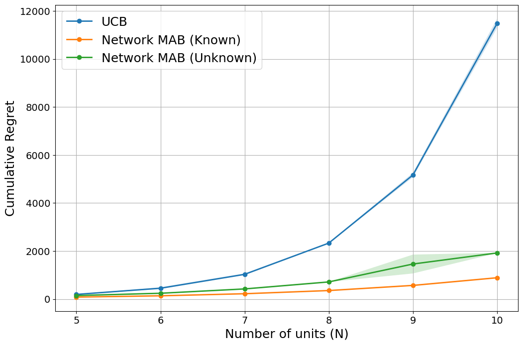
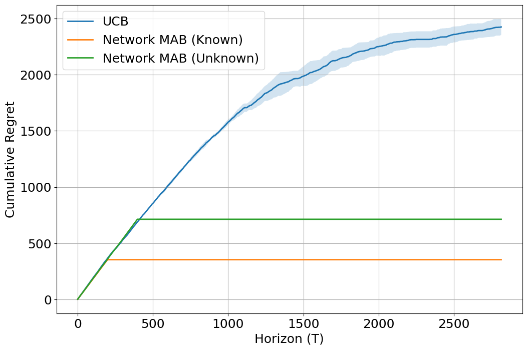
Results. We plot the regret at the maximum horizon time as a function of , and the cumulative regret as we vary for in Figure 2 below. Our results are averaged over repetitions, with shaded regions representing 1 standard deviation measured across repetitions. Algorithms 1 and 2 are denoted by Network MAB (Known) and Network MAB (Unknown) respectively. We discuss both sets of plot separately below.
Regret Scaling with . We plot the cumulative regret when for in Figure 2 (a). Classical MAB algorithms such as UCB see an exponential growth in the regret as increases. Both Algorithm 1 and Algorithm 2 have much milder scaling with . Algorithm 1 uses to reduce the ambient dimension of the regression, hence suffering less dependence on as compared to Algorithm 2.
Regret Scaling with . We plot the cumulative regret for in Figure 2 (b). Despite the poorer scaling of our regret bounds with , our algorithms lead to significantly better regret than UCB which takes a large horizon to converge. Algorithm 1 is able to end its exploration phase earlier than algorithm 2 since it does not need additional samples to learn the sparsity unlike the Lasso.
7 Conclusion
This paper introduces a framework for regret minimization in MABs with network interference, a ubiquitous problem in practice. We study this problem under a natural sparsity assumption on the interference pattern and provide simple algorithms both when the network graph is known and unknown. Our analysis establishes low regret for these algorithms and numerical simulations corroborate our theoretical findings. The results in this paper also significantly generalize previous works on MABs with network interference by allowing for arbitrary and unknown (neighbourhood) interference, as well as comparing to a combinatorially more difficult optimal policy. This paper also suggests future directions for research such as designing algorithms that achieve optimal dependence in without paying any cost in or other problem parameters. Establishing lower bounds to understand optimal algorithms will also be valuable future work. Further extensions could also include considering interference in contextual bandits or reinforcement learning problems. We also hope this work serves as a bridge between online learning and discrete Fourier analysis.
References
- Abbasi-Yadkori et al. (2011) Yasin Abbasi-Yadkori, Dávid Pál, and Csaba Szepesvári. Improved algorithms for linear stochastic bandits. Advances in Neural Information Processing Systems, 24, 2011.
- Abbasi-Yadkori et al. (2012) Yasin Abbasi-Yadkori, David Pal, and Csaba Szepesvari. Online-to-confidence-set conversions and application to sparse stochastic bandits. In Artificial Intelligence and Statistics, pages 1–9. PMLR, 2012.
- Agarwal et al. (2023) Abhineet Agarwal, Anish Agarwal, and Suhas Vijaykumar. Synthetic combinations: A causal inference framework for combinatorial interventions. Advances in Neural Information Processing Systems, 36:19195–19216, 2023.
- Agarwal et al. (2022) Anish Agarwal, Sarah H Cen, Devavrat Shah, and Christina Lee Yu. Network synthetic interventions: A causal framework for panel data under network interference. arXiv preprint arXiv:2210.11355, 2022.
- Aronow (2012) Peter M Aronow. A general method for detecting interference between units in randomized experiments. Sociological Methods & Research, 41(1):3–16, 2012.
- Aronow and Samii (2017) Peter M. Aronow and Cyrus Samii. Estimating average causal effects under general interference, with application to a social network experiment. The Annals of Applied Statistics, 11(4):1912 – 1947, 2017. doi: 10.1214/16-AOAS1005. URL https://doi.org/10.1214/16-AOAS1005.
- Auer et al. (2002) Peter Auer, Nicolo Cesa-Bianchi, and Paul Fischer. Finite-time analysis of the multiarmed bandit problem. Machine Learning, 47:235–256, 2002.
- Bajari et al. (2021) Patrick Bajari, Brian Burdick, Guido W Imbens, Lorenzo Masoero, James McQueen, Thomas Richardson, and Ido M Rosen. Multiple randomization designs. arXiv preprint arXiv:2112.13495, 2021.
- Bajari et al. (2023) Patrick Bajari, Brian Burdick, Guido W Imbens, Lorenzo Masoero, James McQueen, Thomas S Richardson, and Ido M Rosen. Experimental design in marketplaces. Statistical Science, 38(3):458–476, 2023.
- Bhattacharya et al. (2020) Rohit Bhattacharya, Daniel Malinsky, and Ilya Shpitser. Causal inference under interference and network uncertainty. In Uncertainty in Artificial Intelligence, pages 1028–1038. PMLR, 2020.
- Cen et al. (2022) Sarah Huiyi Cen, Anish Agarwal, Christina Yu, and Devavrat Shah. A causal inference framework for network interference with panel data. In NeurIPS 2022 Workshop on Causality for Real-world Impact, 2022.
- Cesa-Bianchi and Lugosi (2012) Nicolo Cesa-Bianchi and Gábor Lugosi. Combinatorial bandits. Journal of Computer and System Sciences, 78(5):1404–1422, 2012.
- Chen et al. (2013) Wei Chen, Yajun Wang, and Yang Yuan. Combinatorial multi-armed bandit: General framework and applications. In International conference on machine learning, pages 151–159. PMLR, 2013.
- Chowdhury and Gopalan (2017) Sayak Ray Chowdhury and Aditya Gopalan. On kernelized multi-armed bandits. In International Conference on Machine Learning, pages 844–853. PMLR, 2017.
- Durand et al. (2018) Audrey Durand, Charis Achilleos, Demetris Iacovides, Katerina Strati, Georgios D Mitsis, and Joelle Pineau. Contextual bandits for adapting treatment in a mouse model of de novo carcinogenesis. In Machine Learning for Healthcare Conference, pages 67–82. PMLR, 2018.
- Even-Dar et al. (2006) Eyal Even-Dar, Shie Mannor, Yishay Mansour, and Sridhar Mahadevan. Action elimination and stopping conditions for the multi-armed bandit and reinforcement learning problems. Journal of Machine Learning Research, 7(6), 2006.
- Gao and Ding (2023) Mengsi Gao and Peng Ding. Causal inference in network experiments: regression-based analysis and design-based properties, 2023.
- Hao et al. (2020) Botao Hao, Tor Lattimore, and Mengdi Wang. High-dimensional sparse linear bandits. Advances in Neural Information Processing Systems, 33:10753–10763, 2020.
- Hudgens and Halloran (2008) Michael G Hudgens and M Elizabeth Halloran. Toward causal inference with interference. Journal of the American Statistical Association, 103(482):832–842, 2008.
- Jia et al. (2024) Su Jia, Peter Frazier, and Nathan Kallus. Multi-armed bandits with interference. arXiv preprint arXiv:2402.01845, 2024.
- Kwon et al. (2017) Joon Kwon, Vianney Perchet, and Claire Vernade. Sparse stochastic bandits. arXiv preprint arXiv:1706.01383, 2017.
- Lattimore and Szepesvári (2020) Tor Lattimore and Csaba Szepesvári. Bandit algorithms. Cambridge University Press, 2020.
- Li et al. (2016) Shuai Li, Alexandros Karatzoglou, and Claudio Gentile. Collaborative filtering bandits. In Proceedings of the 39th International ACM SIGIR Conference on Research and Development in Information Retrieval, pages 539–548, 2016.
- Negahban and Shah (2012) Sahand Negahban and Devavrat Shah. Learning sparse boolean polynomials. In 2012 50th Annual Allerton Conference on Communication, Control, and Computing (Allerton), pages 2032–2036. IEEE, 2012.
- O’Donnell (2014) Ryan O’Donnell. Analysis of boolean functions. Cambridge University Press, 2014.
- Pouget-Abadie et al. (2019) Jean Pouget-Abadie, Kevin Aydin, Warren Schudy, Kay Brodersen, and Vahab Mirrokni. Variance reduction in bipartite experiments through correlation clustering. Advances in Neural Information Processing Systems, 32, 2019.
- Rigollet and Hütter (2023) Philippe Rigollet and Jan-Christian Hütter. High-dimensional statistics. arXiv preprint arXiv:2310.19244, 2023.
- Rosenbaum (2007) Paul R Rosenbaum. Interference between units in randomized experiments. Journal of the American Statistical Association, 102(477):191–200, 2007.
- Rubin (1978) Donald B Rubin. Bayesian inference for causal effects: The role of randomization. The Annals of statistics, pages 34–58, 1978.
- Srinivas et al. (2009) Niranjan Srinivas, Andreas Krause, Sham M Kakade, and Matthias Seeger. Gaussian process optimization in the bandit setting: No regret and experimental design. arXiv preprint arXiv:0912.3995, 2009.
- Ugander et al. (2013) Johan Ugander, Brian Karrer, Lars Backstrom, and Jon Kleinberg. Graph cluster randomization: Network exposure to multiple universes. In Proceedings of the 19th ACM SIGKDD International Conference on Knowledge Discovery and Data Mining, pages 329–337, 2013.
- Vershynin (2018) Roman Vershynin. High-dimensional probability: An introduction with applications in data science, volume 47. Cambridge university press, 2018.
- Wainwright (2019) Martin J Wainwright. High-dimensional statistics: A non-asymptotic viewpoint, volume 48. Cambridge university press, 2019.
- Whitehouse et al. (2024) Justin Whitehouse, Aaditya Ramdas, and Steven Z Wu. On the sublinear regret of GP-UCB. Advances in Neural Information Processing Systems, 36, 2024.
- Yu et al. (2022) Christina Lee Yu, Edoardo M Airoldi, Christian Borgs, and Jennifer T Chayes. Estimating the total treatment effect in randomized experiments with unknown network structure. Proceedings of the National Academy of Sciences, 119(44):e2208975119, 2022.
Appendix A Proof of Proposition 3.1
By the discussion in Section 3, recall that for any action and unit , the reward can be expressed as . To establish the proof, it suffices to show that for any satisfying , . Let be an arbitrary index, then, we have,
where the final equality follows from the fact that, by Assumption 2, when and differ only in positions indexed by . Thus, the only subsets where we can have are those satisfying , which proves the desired result.
Appendix B Proofs for for Known Interference
B.1 Helper Lemmas
Recall the following notation before establishing our results. We defined as the set of indices of the treatment vector belonging to neighbors . Additionally, , where . For a matrix , let denote its minimum singular value. To proceed, we quote the following theorem.
Lemma B.1 (Theorem 5.41 in Vershynin [2018]).
Let such that its rows are independent isotropic random vectors in . If almost surely for all , then, with probability at least , one has
for universal constant .
Lemma B.2 (Minimum Eigenvalue of Fourier Characteristics).
There exists a positive constant such that if , then,
with probability at least .
Proof.
We begin by showing the conditions for Lemma B.1 are satisfied. First, we prove is isotropic, i.e., , where the expectation is taken over uniformly sampling actions uniformly and random from . This follows since for any two subsets ,
Since, for all actions , . Hence, by Lemma B.1, . Next, using the fact that , we get that
Finally, plugging in for an appropriate gives us the claimed result. ∎
We quote the following theorem regarding the error of .
Lemma B.3.
[Theorem 2.2 in Rigollet and Hütter [2023]] Assume that , where is sub-Gaussian, where . If , and covariance matrix has rank , then we have with probability at least ,
where is the least squares estimator, and is a positive universal constant.
While the above lemma bounds the mean-squared error the least-squares estimate, in our applications we can about bounding the distance between and . Simple rearrangement on the above implies that, with probability at least , we actually have
If, in particular, , the above can be simplified to
with probability at least for some new, appropriate universal constant .
B.2 Proof of Theorem 4.1
Proof.
Recall the notation , and . The average reward can be bounded using the definition of and Holder’s inequality as follows,
Using then gives us
| (2) |
Next, define “good” events for any unit as
where is as stated above. Notice that there exists a sufficiently large universal constant , such that implies . Hence, for any given , we have via Lemma B.2 that holds with probability Conditioned on , we get that . Summarizing, we get that for any , the following holds
with probability at least , where is an appropriate constant. Taking a union bound over all units, and then substituting into (2) gives us
Finally, using this, the cumulative regret can be upper bounded with probability as follows:
Substituting as in the theorem statement completes the proof. ∎
Appendix C Proofs for Unknown Interference
In this appendix, we prove Theorem 5.1. Our proof requires the following lemmas.
C.1 Helper Lemmas for Theorem 5.1
The first lemma we prove details the (high-probability) incoherence guarantees of the uniformly random design matrix under the Fourier basis. Recall the following notation before stating and proving our results. We denote as our exploration length, and as the Fourier characteristic associated with action . Let Additionally, we require the following definition of incoherence.
Definition C.1.
We say a matrix is -incoherent if , where is the identity matrix of dimension .
Lemma C.2 (Incoherence of Fourier Characteristics).
For , suppose . Then,
where denotes the maximum coordinates of a matrix. Thus, if , is -incoherent with probability at least .
Proof.
Recall that, for any , , where is some fixed enumeration of subsets . Thus, each entry of can be viewed as being indexed by subsets .
To establish (C.2), we first examine diagonal elements of . For , we have
| (3) |
where the last equality follows from the fact that .
Next, we consider off-diagonal elements, and bound their magnitude. Before doing so, we require the following. For subsets , let denote the symmetric difference of two subsets. For any two subsets , the product of their Fourier characteristics is,
Using this, for any distinct subsets , we have
Since , and , the set of random variables are independent Rademacher random variables. Applying Hoeffding’s inequality for gives us
Applying the inequality above and taking a union bound over all elements of
Choosing yields,
| (4) |
In addition to the above lemma, we leverage the following Lasso convergence result. We state a version that can be found in the book on high-dimensional probability due to Rigollet and Hütter [2023].
Lemma C.3 (Theorem 2.18 in [Rigollet and Hütter, 2023] ).
Suppose that , where , is -sparse, and has independent 1-sub-Gaussian coordinates. Further, suppose is -incoherent. Then, for any and for , we have, with probability at least
where denotes the solution to the Lasso and is some absolute constant.
C.2 Proof of Theorem 5.1
Proof.
Define . Recall the notation , and . For any round , we greedily play the action . The average reward can be bounded using the definition of and Holder’s inequality as follows,
Next, substituting the definition of , , and using the triangle inequality into the equation above gives us,
| (5) |
Let us define the “good” events by
where is the constant following the discussion of Lemma C.3. Let us define the global “good” event by . We show .
First, there is a universal constant such that when . Thus, by Lemma C.2, we know the matrix with as its rows is -incoherent least , i.e. .
Next, conditioning on and applying Lemma C.3 alongside a union bound over the units yields
for all with probability at least , i.e. . Thus, in total, we have . We assume we are operating on the good event going forward.
Plugging the per-unit norms into (5), the cumulative regret can be upper bounded with probability as follows:
| (6) |
Clearly, we should select to roughly balance terms (up to multiplicative constants). In particular, using the choice of as
and substituting into (6) gives us
with probability at least , precisely the claimed result. ∎
Appendix D A Sequential Elimination Algorithm
In both Sections 4 and 5, we presented simple “explore then commit”-style algorithms for obtaining low regret for instances of multi-armed bandits with network interference. The regret bounds for both algorithms had a dependence on the time-horizon that grew as . We noted that, due to strong lower bounds from the sparse bandit literature [Hao et al., 2020], this dependence on was generally unimprovable for the unknown interference case. However, in the known interference setting, there is no reason to believe that the dependence on obtained by Algorithm 1 is optimal. In particular, due to classical results in the multi-armed and linear bandits literature, one would expect the optimal dependence on the time horizon to be . The question considered in this appendix is as follows: can we obtain a -rate regret bound in the presence of known network interference?
To answer this question, we present Algorithm 3, a sequential elimination-style algorithm that attains an improved regret dependence on the time horizon . We caution that, although this algorithm obtains regret, this does not imply it strictly outperforms Algorithm 1. In particular, the regret rate presented in Theorem D.1 has a worse dependence on , the total number of units. For example, when , Algorithm 1 offers a better regret guarantee then Algorithm 3.
We provide some brief intuition for how Algorithm 3 works. The algorithm, which follows the design of the original sequential elimination algorithm for multi-armed bandits due to Even-Dar et al. [2006], operates over multiple phases or epochs. At the start of each epoch, the algorithm maintains a set of “global-feasible” actions which are suspected of offering high reward. Then, during each epoch, the algorithm iterates over each of the units, and uniformly explores the actions of unit and it’s immediate neighbors444that is, the other units on which the outcome of unit depends. that are consistent with some globally-feasible action. Once this exploration phase is complete, actions that are suspected of being sub-optimal are eliminated, and the process repeats.
Theorem D.1.
Proof.
For each , define the “good” event
Observe that standard sub-Gaussian concentration alongside a union bound over units and actions yields that, with probability at least , simultaneously for all and ,
In other words, . Now, define the global “good” event
and define . On the event , we have
and thus we have the inclusion . Performing a union bound over the epochs yields that
We assume we are operating on this “good” event throughout the remainder of the proof. On , we observe that (a) the optimal action satisfies for all , as we have
where we have set to be any action obtaining the mean estimate , and (b) for all , which holds by an analogous argument.
Now, letting be an arbitrary time horizon, and define to be a lower bound on the largest epoch index to have started by time . We claim that . In fact, we have
where the third inequality follows from the fact for all and .
Now, we have everything we need to put together a regret bound. Still operating on the good event , we have
∎