Stability of the Rao–Nakra sandwich beam with a dissipation of fractional derivative type: theoretical and numerical study
Abstract.
This paper is devoted to the solution and stability of a one-dimensional model depicting Rao–Nakra sandwich beams, incorporating damping terms characterized by fractional derivative types within the domain, specifically a generalized Caputo derivative with exponential weight. To address existence, uniqueness, stability, and numerical results, fractional derivatives are substituted by diffusion equations relative to a new independent variable, , resulting in an augmented model with a dissipative semigroup operator. Polynomial decay of energy is achieved, with a decay rate depending on the fractional derivative parameters. Both the polynomial decay and its dependency on the parameters of the generalized Caputo derivative are numerically validated. To this end, an energy-conserving finite difference numerical scheme is employed.
Key words and phrases:
Rao–Nakra sandwich beam, fractional derivative, numerical polynomial stability2010 Mathematics Subject Classification:
35A01, 35A02, 35M33, 93D20, 34B05, 34D05, 34H05, 35B40, 74K20, 74F051. Introduction
In 1999, Liu, Trogdon and Yong [28] developed the following general three-layer laminated beam–plate model:
| (1.6) |
The physical parameters are the thickness, density, Young’s modulus, shear modulus and moments of inertia of the -th layer for from bottom to top, respectively. In addition, and
The Rao–Nakra sandwich beam model [45] is the following:
| (1.13) |
with and Here and are the longitudinal displacement. is the transverse displacement of the beam. This system is derived from the system (1.6) when we consider the core material to be linearly elastic, that is, with the shear strain
where the shear modulus and is the Poisson ratio.
Many authors have been working on the system (1.13) from different points of view: see [27, 39, 40, 46] and the references therein. In the past three decades there has been a growing interest by many reserchers for the study of fractional calculus in different fields of sciences [32, 48, 49]. Several aspects of engineering, applied sciences, and mathematical physics benefitted from this ascending wave of applications. Space sciences, fluid mechanics, porous media flows, viscoelastic and biological processes are but a few areas in which fractional order differential equations have become a favored tool to tread new path. To give some examples, fractional derivatives have been used to model frequency dependent damping behavior of many viscoelastic materials as well modeling many chemical processes. Many problems in several scientific applied areas, including the analysis of viscoelastic materials, heat conduction in materials with memory, electrodynamics with memory, signal processing, among others, can be modeled by fractional differential calculus. Indeed, many investigations have shown that models involving fractional derivatives are more realistic to represent some natural phenomena than models involving classical derivatives. For more information we refer to [24, 34, 47] and the references therein. For example, the wave equation with boundary fractional damping has been treated in [34, 35] where the strong stability and the lack of uniform stabilization were proved. Applications of this kind are also found in [33, 36, 42, 44, 50] and the references therein.
In [50] the authors studied the Rao–Nakra system with a boundary dissipation of fractional derivative type. They established the polynomial stability of the system. In this article we are interested in studying the polynomial stabilization to the system (1.22) from a theoretical and numerical point of view. In order to achieve this, we eliminate the dissipation given on the border and place the dissipation in the domain. The main idea to reach this result is to use an idea given in [4]. It is important to note that the imposed dissipation is of a fractional derivative type. Our method is based on the fact that the input–output relationship in a certain diffusion equation introduced by Mbodje in [34] is realized by a fractional derivative operator.
Numerical approximations of derivatives and fractional integrals have been extensively studied, developed, and refined. Comprehensive reviews on this topic are available in [11, 26]. Many of these approaches involve direct approximations of the Riemann–Liouville, Caputo [18, 31, 13, 14, 15], or Grünwald–Letnikov integral [26], using quadrature methods, finite differences, and truncated summations [19]. While some progress has been made in enhancing the convergence rate, such as through trapezoidal approximation [26] or spline interpolation [17], these methods do not inherently preserve the energy conservation property of the Rao–Nakra model under study, nor do they maintain stability in the presence of dissipative terms. In this work, we address this challenge by employing a suitable combination of the -Newmark method [38], coupled with a Crank–Nicolson method for the Mbodje diffusion equation, to achieve our objective.
Without lost of generality, we will consider the following system for :
| (1.22) |
with , and real-valued functions and .
The rest of the paper is divided into five sections. In Section 1 we show that the system (1.22) may be replaced by an augmented system (2.28) obtained by coupling an equation with a suitable diffusion, and we study the energy functional associated to system. In Section 3, we establish the existence and uniqueness of solutions of the system (2.28); for this we use [5, 4]. In section 4 we prove the strong stability, the lack of uniform stabilization and the polynomial stability of the system (2.28). In Section 5, we give a numerical study of the polynomial stability.
Throughout this paper, is a generic constant, not necessarily the same at each occasion (it may change from line to line) and depending on the indicated quantities.
2. Augmented Model
This section is devoted to the reformulation of the model (1.22) with boundary conditions (1.22)7, 8 as an augmented system. First we provide a brief review of fractional calculus. There are many definitions of fractional derivatives [18], among them those of Riemann–Liouville and Caputo are the most widely used [31]. The latter has the same Laplace transform as the integer order derivative, so it is widely used in control theory. In this paper the fractional derivative damping force is regarded as a control force to study the properties of free damped vibrations of the system, hence the Caputo definition [13, 14, 15] is used here. Let . The Caputo fractional integral of order is defined by the formula
| (2.1) |
where is the Gamma function, and
The Caputo fractional derivative operator of order is
defined by the expression
| (2.2) |
The Caputo definition of fractional derivative possesses a very simple but interesting interpretation: if the function represents the strain history within a viscoelastic material whose relaxation function is , then the material will experience at any time a total stress given by the expression Also, it easy to show that is a left inverse of but in general it is not a right inverse. More precisely, we have
See [47] for the proof of above equalities and for more properties of fractional calculus.
In this work, we consider a slightly different version of (2.1) and (2.4). In [16], Choi and MacCamy introduced the following definition of fractional integro-differential operators with an exponential weight. Given and , the exponential fractional integral of order is defined by
| (2.3) |
and the exponential fractional derivative operator of order is defined by
| (2.4) |
Note that
We will need later the following results:
Theorem 2.1.
[34] Let be the function
| (2.5) |
Then the relation between the Input and the Output is given by the following system:
| (2.6) | |||
| (2.7) | |||
| (2.8) |
This implies that
| (2.9) |
where
Lemma 2.2.
[1, Lemma 2.1] If , then
Our strategy requires the elimination of the fractional derivatives in time from the domain condition in the system (1.22). To this, setting and exploiting the technique from [21], we reformulate the system (1.22) by using Theorem 2.1. This leads to the following augmented model, where and we introduce the constant :
| (2.28) |
3. Setting of the Semigroup
In this section, we discuss the existence and uniqueness of solutions for the coupled system (2.28) by the semigroup theory [41, 43].
We will use the standard space; the scalar product and the norm are denoted by
We introduce the Hilbert space
| (3.1) | |||||
equipped with the following inner product:
| (3.2) |
where and We wish to transform the initial boundary value problem (2.28) into an abstract Cauchy problem in the Hilbert space For this we introduce the functions and we rewrite the system (2.28) as the following initial value problem:
| (3.3) |
Here is as above, and the operator is given by the formula
| (3.4) |
with the domain
Let the operator which is given by
| (3.5) |
with the domain
.
We note that the operator is self-adjoint and strictly positive.
| (3.6) |
where and
We define
| (3.7) |
equipped with the inner product given by
| (3.8) |
where and
Then, the operator given by
| (3.9) |
with the domain
Proposition 3.1.
The energy of the solution of the system (3.18) is defined as follows:
| (3.19) |
and it is decreasing function of the time In particular, we have
| (3.20) |
Proposition 3.2.
The energy of the system (3.18), defined by
| (3.21) |
is decreasing in time In particular, we have
| (3.22) |
4. Non-uniform stabilization
4.1. Polynomial stability for
Assume that then the operator is not onto and consequently the resolvent set of
Since the embedding is compact and the only solution of the following problem:
| (4.10) |
is the trivial one.
To determine the rate of stability in this case, we need the following result [7, Theorem 8.4]:
Theorem 4.1 ([7]).
Let be a bounded C0-semigroup on a Hilbert space with generator Assume that and that there exist such that
Then, there exists a constant such that
where is the domain of and is the range of
Based on Theorem 4.1, a simple adaptation of the proofs of [8, Theorems 5.8 and 5.9] (see also [4, 5]) lead to the following stability result:
Proposition 4.2.
If , then there exists a such that
| (4.11) |
where is the range of
4.2. Polynomial stability for
5. Numerical study
In this section we will verify numerically the polynomial rate of decay obtained in the previous section.
5.1. Linear equations of Motion
First, we approximate the longitudinal and transverse displacement vector in space using an energy-conservative finite difference method. For and , we define , with , as a uniform discretization of the interval , obtaining a vector approximation of in . We obtain the linear equation of motion
| (5.1) |
where is the generalized Caputo fractional derivative defined in (2.2). In addition, and according to a discretization consistent with (1.22), we choose (identity matrix). The stiffness matrix is given by , where
Here, and are the finite difference matrix approximation of and respectively with the boundary conditions (1.22)7,8, and is the upper triangular matrix, obtained from the Cholesky decomposition . Using uniform finite differences we have
According to the boundary conditions (1.22)7,8, we seek the solution of Finite Difference in
considering .
5.2. Time discretization
In order to preserve the energy with a second order scheme in time, we choose a -Newmark scheme for . The method consists of updating the displacement, velocity and acceleration vectors at the current time to the time , a small time interval later. The Newmark algorithm [38] is based on a set of two relations expressing the forward displacement and velocity in terms of their current values and the forward and current values of the acceleration:
| (5.2) | |||||
| (5.3) |
where and are parameters of the methods that will be fixed later. Replacing (5.2)–(5.3) in the equation of motion (5.1), we obtain
| (5.4) |
5.3. Approximation of fractional derivatives
At this state we have two possibilities: (1) approximate the fractional derivative using a classical finite difference method such as the truncation of the Grünwald–-Letnikov derivative [19], which in turn is an equivalent form of the Riemann–Liouville derivative; or, (2) propose a conservative numerical scheme for the Mbodje augmented model (2.28).
5.3.1. Approximation using a truncation of the Grünwald-–Letnikov derivative.
5.3.2. Approximation using the Mbodje augmented model
On the other hand, in case of the Mbodje augmented model (2.28) we propose the following conservative numerical scheme:
| (5.8) |
where , with denoting the approximation of evaluated in and , for , and a fixed . Using (5.2) again and replacing in (5.8)2, we can rewrite (5.8) in the following more explicit and computable way:
| (5.9) |
where , and . Although the two approximations are consistently valid from the point of view of finite differences, we will opt for the second approximation because it conserves the energy in the non-dissipative case, and its decrease is consistent with the continuous case. It also involves the calculation of which is inherent to the definition of energy itself.
5.4. Decay of the discrete energy using the Mbodje augmented model
Evaluating (5.8)1 in , multiplying by , and summing (5.8)2 multiplied by , we obtain that
| (5.10) | |||||
which is consistent with the estimates (3.21)–(3), and constitutes a correct approximation of the energy and its decreasing behavior.
Remark 5.1.
In the case of an approximation using a truncation of theGrünwald–-Letnikov derivative, we have the following estimate of the energy. Evaluating (5.1) in and multiplying by we obtain
| (5.11) | |||||
where . The first term on the right hand side of (5.11) is obviously strictly negative. However, the sign of the second and third terms in (5.11) cannot be guaranteed. In fact, it is verified numerically that the energy discretized in this way is not necessarily strictly decreasing, unless the solution is sufficiently smooth and delta t is small enough.
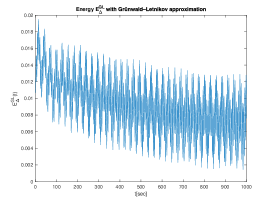
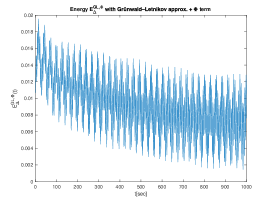
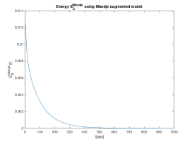
Figure 1 shows a comparison of both models. It is proved that the calculation of energy using the classical Grünwald–-Letnikov derivatives fails, either by using the derivative defined in (5.11), (in top left graph), as well as by artificially adding the calculation of as seen in the top right graph. Therefore, the only acceptable method for all our calculations should be the discretization of the augmented Mbodje model (bottom graph).
5.5. Numerical examples
We consider here the value of the parameters , a beam of length , and the initial conditions
| (5.12) |
We observe that and is of class but its second derivative has a discontinuity in , and in turn, with of class and its fourth derivative has a discontinuity at . Therefore, we have just , but no greater regularity than that.
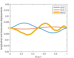
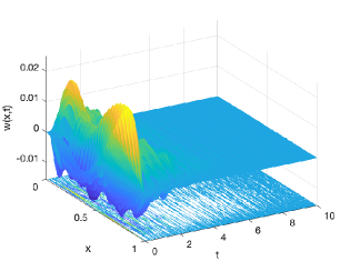
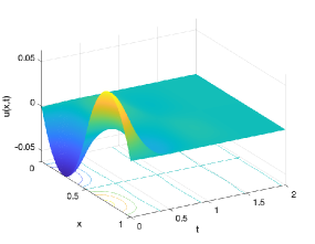
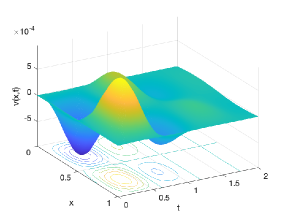
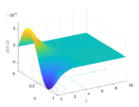
In Figure 2, we consider a fractional derivative with , and we do a simulation of the numerical scheme (5.2), (5.3), (5.7) with , and with and . The graphs in (A) of Figure 2 shows the state of the instant of the deformations for . The beam is represented by the thick yellow graph and its deformation corresponds to the transversal displacements. The longitudinal displacements of and , are represented by the blue and red lines respectively. The graph (B) of the figure 2 shows the evolution of the transverse displacements in term of space and time. Graphs (C) and (D) of the same figure show the longitudinal displacements and (respectively), also as a function of space and time. In this set of figures, the decay of the quantities, and therefore of the energy, is visually observed due to the dispative terms of the fractional derivative type.
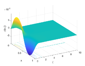
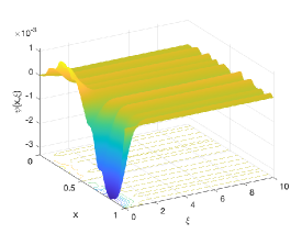
On the other hand, we show in figure 3 the graphs of the numerical variables that approximate the auxiliary functions , , and of the augmented model (2.28), for the instant of the simulations with the same parameters and data as the example in figure 2. We numerically observe a decay of these functions with respect to the variable , although not so evident in the case of the variable associated with the term of the fractional derivative of the transverse displacement (when truncating at ). In this sense, we must be careful with the numerical truncation of the variable . For this reason we will consider a truncation at for the examples that will follow, and that will show the polynomial decay of energy for different values of and .
regrouped in terms of the values of .
and different values of
with a same as a function of time,
and their asymptotes

with a same as a function of time,
and their asymptotes
| 0.01 | 0.25 | 0.50 | 0.75 | 0.99 | ||
|---|---|---|---|---|---|---|
Finally, in order to numerically appreciate the polynomial decay of the energy, we do the simulation with the same parameters , a beam of length , and the initial conditions (5.12), but for a longer time , and a time step . Likewise, in order to obtain better precision in the results, we truncate the variable of the auxiliary functions at .
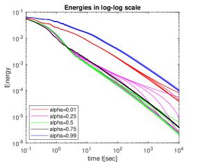
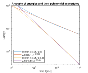
In Figure 4, various plots depict energy on a log-log scale, where curves of the form exhibit nearly linear behavior over sufficiently long times.
The graph in Figure 4(A) illustrates energy curves for 9 different values of and 5 values of , totaling 45 combinations. Similar curves with the same are grouped into 5 distinct colors. While there are variations in slopes and constants , graphical observation reveals a close relationship between these parameters, particularly in their bounded ranges. The numerical estimation of and using a least squares method is presented in Table 1.
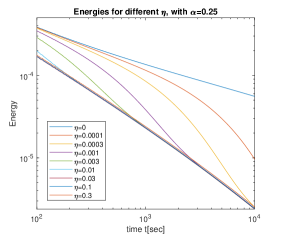
Additionally, from the graph, it is conjectured that energy decays more rapidly to zero for (or similar values) and certain . Conversely, exhibits intriguing behavior, accentuating differences across various values. Thus, the curves corresponding to are separately plotted in Figure 4(B). Here, a pattern emerges with curves lying between two quasi-linear lines with distinct slopes. The steepest negative slope corresponds to , while the smallest absolute slope corresponds to , with intermediate values approaching the former asymptotically.
Figures 4(C) and 4(D) compare energy curves with their respective asymptotic forms resembling straight lines in a log-log graph. These asymptotic curves, of the form , are derived through least squares, effectively capturing the data’s behavior. In Figure 4(C), distinct values for the same exhibit notably different slopes (i.e., decay rates ). Conversely, in Figure 4(D), variations in the multiplicative constant outweigh changes in the decay rate across different values.
Discussion and Conclusions
We have demonstrated the existence, uniqueness, and stability of a Rao–Nakra model with dissipative terms of the generalized Caputo fractional derivative type within the domain, building upon ideas from a proven case for a broader class of evolution systems [4]. While focusing on the Rao–Nakra beam model, our treatment of the fractional term through an input–output relationship with a diffusion equation [34] has illuminated a numerical method of finite-conservative differences type that ensures stable energy decay, unlike standard methods for approximating fractional derivatives. This enabled us to numerically simulate energy decay, confirming its polynomial nature.
One key observation from the data and interpretation of Figure 4 and Table 1 is the clear asymptotic polynomial decay behavior of energy. We note that the decay rate is notably greater in absolute value when , and lower when , validating the theoretical propositions (Proposition 4.3 and Theorem 4.2). However, we acknowledge discrepancies between the theoretically derived rates and the numerically estimated ones. We attribute this to factors such as the discretization step sizes and , the order of convergence of the method introducing additional numerical dissipation, and the limited simulation times for observing true theoretical decay rates.
Future work should delve into numerical methods enhancing convergence order to obtain numerical values closer to theoretical ones. Additionally, exploring inverse or control problems, such as identifying parameter pairs for quicker energy decay, merits attention. Notably, from Table 1, we observe a minimum in the rate near . An inverse problem could involve minimizing this slope with respect to . Moreover, considering the importance of the constant , as evidenced by the curve nearest to zero at corresponding to in Figure 4(A), remains intriguing.
However, beyond , maintaining a constant to ensure optimal decay is unclear. While minimizing energy decay speed is of interest, defining a suitable cost function characterizing this decay speed requires further exploration. Thus, identifying the appropriate cost function to minimize for solving the inverse problem remains an open task.
References
- [1] Z. Achouri, N.E. Amroun and A. Benaissa, The Euler-Bernoulli beam equation with boundary dissipation of fractional derivative type. Methods Appl. Sci. 40 (2017), no.11, 3837–3854.
- [2] R.A. Adams. Sobolev Spaces. Academic Press,New York. 1975.
- [3] M.S. Alves, J.E. Muñoz Rivera, M. Sepúlveda, O. Vera. Exponential stability in thermoviscoelastic mixtures of solids. I. J. Solid Struct., 46 (2009), 4151–416.
- [4] K. Ammari, H. Fathi, L. Robbiano. Fractional-Feedback stabilization for a class of evolution systems. J. Differential Equations. 268 (2020), 5751–5791.
- [5] K. Ammari, F. Hassine, L. Robbiano, Stabilization for Some Fractional-Evolution Systems. SpringerBriefs in Mathematics. Springer, Cham, 2022.
- [6] C.J.K. Batty and T. Duyckaerts. Non-Uniform stability for bounded semi-groups on Banach spaces. J. Evol. Equ. (2008), 765–780.
- [7] C.J.K. Batty, R. Chill, Y. Tomilov, Fine scales of decay of operator semigroups. J. Eur. Math. Soc., 18 (2016), 853–929.
- [8] A. Benaissa, A. Boudaouad, Some results on the energy decay of solutions for a wave equation with a general internal feedback of diffusive type. Advances in Partial Differential Equations and Control. Trends Math. Birkhäuser/Springer, Cham, 2024.
- [9] A. Borichev, Y. Tomilov. Optimal polynomial decay of functions and operator semigroups. Math. Ann., Vol. 347. 2 (2010), 455–478.
- [10] N. Burq. Décroissance de l’energie locale de l’équation des ondes pour le problème extérieur et absence de résonance au voisinage du réel. Acta Math. (1998), 1–29.
- [11] M. Cai, C. Li. Numerical approaches to fractional integrals and derivatives: A review. Mathematics, Vol. 8(1), 43 (2020).
- [12] X.-G. Cao, D.-Y. Liu, G.-Q. Xu. Easy test for stability of laminated beams with structural damping and boundary feedback controls. J. Dyn. Control Syst. Vol. 13. 3 (2007), 313–336.
- [13] M. Caputo. Linear models of dissipation whose Q is almost frequency independent Part II. Geophys. J. R. Astr. Soc.
- [14] M. Caputo. Elasticità e Dissipazione. Zanichelli, Bologna (1969). (in Italian: Elasticity and Dissipation).
- [15] M. Caputo, F. Mainardi. Linear models of dissipation in anelastic solids. Riv. Nuovo Cimento. (Ser. II) 1 (1971), 161–198.
- [16] J. Choi, R. Maccamy. Fractional order Volterra equations with applications to elasticity. J. Math. Anal. Appl., 139 (1989), 448–464.
- [17] M. Ciesielski. Numerical Algorithms for Approximation of Fractional Integrals and Derivatives Based on Quintic Spline Interpolation. Symmetry, 16(2), 252 (2024).
- [18] S. Das. Functional Fractional Calculus for System Identification and Control. Springer Science & Business Media, 2011.
- [19] M. Duarte Ortigueira, F. Coito From Differences to Derivatives. Fractional Calculus and Applied Analysis. 7 (2004) 459–471.
- [20] L.M. Gearhart. Spectral theory for contraction semigroups on Hilbert spaces. Trans. Amer. Math. Soc. 236 (1978), 385–394.
- [21] F.L. Huang. Characteristic condition for exponential stability of linear dynamical systems in Hilbert spaces. Ann. Diff. Eqns., Fuzhou. 1 (1985), 43–56.
- [22] S.W. Hansen, R. Spies. Structural damping in a laminated beams due to interfacial slip. J. Sound Vib. 204 (1997), 183–202.
- [23] S.W. Hansen. In Control and Estimation of Distributed Parameter Systems: Non-linear Phenomena. International Series of Numerical Analysis. ISNA 118(1994)143-170. Basel: Birkhaser. A Model for a two-layered plate with interfacial slip.
- [24] A. Kilbas, H. Srivastava, J. Trujillo. Theory and Applications of Fractional Differential Equations. North-Holland Mathematics Studies, 204. Elsevier Science B.V., Amsterdam, 2006.
- [25] V. Komornik. Exact controllability and stabilization: The multiplier method. John Wiley & Sons. 1994.
- [26] C. Li, F. Zeng. Numerical Methods for Fractional Calculus. Boca Raton FL: CRC Press Taylor & Francis Group; 2015.
- [27] Z. Liu, B. Rao, Q. Zheng. Polynomial stability of the Rao-Nakra beam with a single internal viscous damping. J Differential Equations. Vol. 269 (2020), 6125-6162.
- [28] Z. Liu, S.A. Trogdon, J. Yong. Modeling and analysis of a laminated beam. Comput Math Model. Vol.30. (1-2)(1999), 149–167.
- [29] Z. Liu, S. Zheng. Semigroups associated with dissipative systems. New York: Chapman & Hall/CRC. 1999.
- [30] A. Lo, N-E Tatar. Stabilization of laminated beams with interfacial slip. EJDE. 129 (2015), 1–14.
- [31] J.A. Machado, I.S. Jesus, R. Barbosa, M. Silva, C. Rei. Application of fractional calculus in engineering, in: Dynamics, Games and Science I. 1 (2011), 619–629.
- [32] R.L. Magin. Fractional Calculus in Bioengineering. Begell House. Redding. CT. USA. 2006.
- [33] T. Maryati, J. E. Muñoz Rivera, V. Poblete, O. Vera. Asymptotic behavior in a laminated beams due interfacial slip with a boundary dissipation of fractional derivative. Applied Mathematics and Optimization. 84 (2021), 85–102.
- [34] B. Mbodje. Wave energy decay under fractional derivative controls. IMA J. Math. Contr. Inform. 23 (2006), 237–257.
- [35] B. Mbodje, G. Montseny. Boundary fractional derivative control of the wave equation. IEEE Trans. Autom. Control. 40 (1995), 378–382.
- [36] J. E. Muñoz Rivera, V. Poblete, O. Vera. Stability for an Klein-Gordon equation type with a boundary dissipation of fractional derivative type. Asymptotic Analysis. Vol. 127. 3 (2022), 249–273.
- [37] M. Nakao. On the decay of solutions of some nonlinear dissipative wave equations. Math. Z. Berlin. 193 (1986), 227–234.
- [38] N.M. Newmark. A method of computation for structural dynamics. J. Engrg. Mech. Div., ASCE 85 (1959).
- [39] A. Ozkan ozer, S.W. Hansen. Uniform stabilization of a multilayer Rao-Nakra sandwich beam. Evol. Equ. Control Theory. Vol. 2 (2013), 695–710.
- [40] A. Ozkan Ozer, S.W. Hansen. Exact boundary controllability results for a multilayer Rao-Nakra sandwich beam. SIAM J Control Optim. Vol. 52 (2014), 1314–1337.
- [41] A. Pazy. Semigroups of Linear Operators and Applications to Partial Differential Equations. Springer- Verlag, New York, 1983.
- [42] V. Poblete, F. Toledo, O. Vera. Polynomial stability for a Piezoelectric beam with magnetic effect with magnetic effect and a boundary dissipation of fractional derivative type. Proceedings of the Edinburgh Mathematical Society. In press.
- [43] J. Prüss. On the spectrum of C0-semigroup. Trans. Am. Math. Soc. 248 (1984), 847–867.
- [44] J.A. Ramos, C. Nonato, C.A, Raposo, O. Vera. Stability for a weakly coupled equations with a boundary dissipation of fractional derivative type. Rendiconti del Circolo Matematico di Palermo Series 2. (2021) doi.org/10.1007/s12215-021-00703-w .
- [45] Y.V.K.S Rao, B.C. Nakra. Vibrations of unsymmetrical sanwich beams and plates with viscoelastic cores. J Sound Vibr. Vol. 34. 3 (1974), 309-326.
- [46] C.A. Raposo, O. Vera, J. Ferreira, E. Piskin. Rao–Nakra sandwich beam with second sound. Partial Differential Equations in Applied Mathematics. 4 (2021), 100053.
- [47] S. Samko, A. Kilbas, O. Marichev. Integral and Derivatives of Fractional Order. Gordon Breach, New York. 1993.
- [48] V.E. Tarasov. Fractional Dynamics: Applications of Fractional Calculus to Dynamics of Particles, Fields and Media. Springer. Berlin/Heidelberg. Germany. 2011.
- [49] D. Valério, J.A.T. Machado, V. Kiryakova. Some pioneers of the applications of fractional calculus. Fract. Calc. Appl. Anal. 17 (2014), 552–578.
- [50] O. Vera, C.A., Raposo, Carlos A. Nonato, Anderson J.A. Ramos. Stability of solution for Rao-Nakra Sandwich beam with boundary dissipation of fractional derivative type. Journal of Fractional Calculus and Applications. Vol. 13. 2 (2022), 116–143.
- [51] M. Walter. Dynamical System and evolution Equations, Theory and Applications. Plenum Press. New York. 1980.
- [52] J.-M. Wang, G.-Q. Xu, S.-P. Yung. Exponential stabilization of laminated beams with structural damping and boundary feedback controls. SIAM J. Control Optim. Vol. 44. 5 (2005), 1575–1597.