From Conformal Predictions to Confidence Regions
Abstract
Conformal prediction methodologies have significantly advanced the quantification of uncertainties in predictive models. Yet, the construction of confidence regions for model parameters presents a notable challenge, often necessitating stringent assumptions regarding data distribution or merely providing asymptotic guarantees. We introduce a novel approach termed CCR, which employs a combination of conformal prediction intervals for the model outputs to establish confidence regions for model parameters. We present coverage guarantees under minimal assumptions on noise and that is valid in finite sample regime. Our approach is applicable to both split conformal predictions and black-box methodologies including full or cross-conformal approaches. In the specific case of linear models, the derived confidence region manifests as the feasible set of a Mixed-Integer Linear Program (MILP), facilitating the deduction of confidence intervals for individual parameters and enabling robust optimization. We empirically compare CCR to recent advancements in challenging settings such as with heteroskedastic and non-Gaussian noise.
1 Introduction
To ensure the safe deployment of machine learning technologies, it is essential to have reliable methods for quantifying uncertainties when making data-driven predictions. Bayesian methods (Bernardo and Smith, 2009), for example, rely on posterior distribution to model these uncertainties. The process begins with a prior distribution that represents prior knowledge before data are observed. Bayes’ rule is then used to obtain a data-dependent probability called the posterior distribution, which represents the updated belief conditional on the data. The resulting distribution is commonly used to measure the likelihood of a specific outcome. However, a good choice of the prior is required in order to have reliable uncertainty estimates, which is difficult without stronger assumptions; see (Castillo, 2024).
Another common approach is to analyze the distribution of prediction errors and use it to create an interval by setting a threshold for the distance between the target and the prediction at a suitable quantile level. However, it is challenging to obtain a closed-form distribution for most prediction algorithms. Standard guarantees are achieved by limiting the analysis to situations where prediction errors can be modelled using a normal distribution e.g when applying the maximum likelihood principle (Van der Vaart, 2000). Similarly, non-parametric approach (Tsybakov, 2009) or Bootstrap confidence sets are only valid in the asymptotic regime or under strong regularity assumptions on the distribution; see (Wasserman, 2006, section 3.5) to estimate convergence rates. Overall, the current guarantees require strong regularity assumptions on the underlying distribution of the data or are only valid asymptotically. Our objective is to depart from these classical regularity assumptions and construct confidence regions in the parameter space that have a probabilistic guarantee of containing the true parameters. In the real world, data is limited and the noise can take unknown, heteroskedastic functional forms. Our confidence regions should possess:
finite-sample validity under minimal assumptions on the data distribution.
Conformal Prediction (CP) methods (Shafer and Vovk, 2008), provide a set of plausible values for the output with a given input . Unlike preceding methodologies, its uncertainty set is valid with finite sample sizes and under the sole assumption that one has access to similarly sampled data whose joint distribution is permutation invariant e.g., iid. Nevertheless, CP offers limited to no insights into the underlying data generation process. Specifically, if is sampled from a parameterized distribution , how can we obtain a confidence set for the true parameter under similarly mild assumptions?
Background
We consider an explicit relationship between the input and output data
| (1) |
where the input takes values in , while the target (or output) and the noise take values in . We denote the ground truth parameter of the model. Conformal prediction builds uncertainty sets for the noisy observation for any tolerance level, i.e. CP builds a set-valued mapping such that
| (2) |
where the probability is taken over , and the observed batch which is used to construct ; it is typically a training sample of the data.
We additionally consider a separate unlabelled sample of size of the data Our goal is now to construct a confidence region over the parameter space such that
| (3) |
In practice, the distribution of the noise is unknown; and assumptions about it is a modeling question, which inherently varies based on the analyst’s methodology and prior knowledge about the underlying phenomena being studied. Popular settings where the noise can be supposed gaussian with identifiable (unique) ground-truth is well studied. Standard solutions based on central limit theorem offers accurate confidence sets valid both in asymptotic and finite sample regime. Recent work (Wasserman et al., 2020b) propose a significant extension by assuming continuous noise and availability of a likelihood function i.e. knowing explicitly the shape of the distribution. Significant research efforts have been dedicated to modeling phenomena with heavy-tailed characteristics, wherein the noise lacks finite moments, rendering classical methods reliant on the central limit theorem inapplicable. Examples include the Voigt profile, which results from convolving a Cauchy distribution with a Gaussian distribution, with applications in physics (Balzar, 1993; Chen et al., 2015; Pagnini and Mainardi, 2010; Farsad et al., 2015). Similarly, the Slash distribution, (Rogers and Tukey, 1972; Alcantara and Cysneiros, 2017), is instrumental for simulating heavy-tailed phenomena. In summary, these methods are designed to model uncertainty yet are fundamentally dependent on properties of the noise that are themselves uncertain. This apparent contradiction calls into question their validity in real-world settings, and motivates our proposed methodology.
Contributions
We summarize our contributions as follows:
-
1.
We extend the validity of conformal prediction methodologies to build uncertainty sets for the noise-free output .
-
2.
We introduce Conformal Confidence Regions (CCR), a method to aggregate the CP intervals of multiple unlabelled inputs to construct a confidence region for the ground-truth parameter .
-
3.
With minimal assumptions on the noise, we provide finite-sample valid coverage guarantees for CCR when the CP intervals are constructed by a black-box methodology, and improved guarantees when the CP intervals originate from the usual split CP method.
-
4.
We propose an approach for regression with abstention leveraging our uncertainty estimation, and we provide finite sample valid probability bounds.
-
5.
We validate CCR empirically by constructing confidence regions for the parameter of a linear distribution under challenging noise distributions, and compare to recent methodologies.
Theoretical proofs of our results are all provided in Appendix C.
2 Confidence Set for Noise-free Outputs
The building blocks of CCR are prediction intervals with finite-sample coverage over the noise-free outputs . In contrast, CP only provides coverage guarantees over the noisy output . We show that the prediction intervals of CP also have coverage guarantees for the noise-free outputs.
Assumption 2.1.
The prediction set is an interval satisfying Equation 2 for some . For conformal prediction sets that aren’t intervals, we consider their convex hull instead.
We define the noise dependent quantity that describes class of distribution we can handle:
Assumption 2.2.
We suppose .
Symmetric noise (e.g. Gaussian) as in (Csaji et al., 2015), implies . It is sufficient for to have a median of everywhere to ensure . Our approach, which provides coverage guarantees based on , offers greater flexibility regarding data distribution compared to previous methods. Intuitively, reflects the tolerance for model misspecification, with guarantees deteriorating as decreases. An issue with classical approaches arises when the noise distribution’s mean does not exist. Distributions lacking a mean still possess quantiles and our primary assumption is a bound on the quantile (e.g., median ), without assuming zero mean noise. Examples as the Cauchy distribution, with infinite variance, makes the central limit theorem inapplicable, yet our methods remain valid. {restatable}propositionnoisefreecov Under the model in Equation 1, 2.1 and 2.2, it holds
| (4) |
2.2 extends conformal guarantees to noise-free outputs, albeit with reduced coverage. Surprisingly, noise-free coverage can be lower than with noise due to adversarial scenarios where often narrowly misses (we provide an explicit example in Section D.1). Empirical evidence (Table 2, Table 6) consistently shows covers more frequently. Across several CP methods, training sizes, noise distributions, and thousands of trials, there is not a single trial for which the noise-free output obtains lower coverage than . Similar observations from Feldman et al. (2023) is that CP with noisy labels attain conservative risk over the clean ground truth labels. This motivates 2.3, a stronger but realistic alternative to 2.2.
Assumption 2.3.
The noise-free outputs have the same coverage guarantee as the noisy outputs,
| (5) |
|
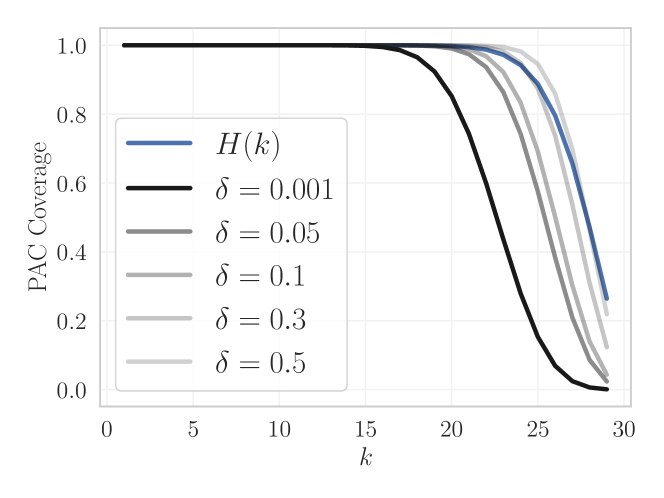
![[Uncaptioned image]](/html/2405.18601/assets/x1.png) Figure 1: Guaranteed coverage of as a function of from the lower bounds in Section 3, under 2.3, with . The dashed line corresponds to the PAC bounds with . In the case of Markov, we can sample uniformly in without loss of guarantee so we are only plotting the coverage against the worst-case .
Figure 1: Guaranteed coverage of as a function of from the lower bounds in Section 3, under 2.3, with . The dashed line corresponds to the PAC bounds with . In the case of Markov, we can sample uniformly in without loss of guarantee so we are only plotting the coverage against the worst-case .
|
3 Confidence Set for the Model Parameter
Having established a confidence set for noise-free outputs, extending it to model parameters involves selecting all the parameters that result in the same confidence interval. Intuitively, this allows us to propagate uncertainty set from the outputs to the underlying model parameters. We define
While having finite sample validity under weak assumption on the noise, the set might be large. For linear models, , we obtain which is unbounded for dimension larger than . A potential strategy would be to leverage each input that yields a valid confidence set . The most straightforward method for combining confidence sets from different test points is to intersect them. As such, we define
Without additional structural assumptions, one can employ the Bonferroni inequality to control the probability of the intersection: . This results in a -confidence set and thus the coverage decreases rapidly with the number of points in .
Aggregation by Voting
To aggregate the more efficiently, we draw inspiration from (Cherubin, 2019; Gasparin and Ramdas, 2024) and (Guille-Escuret and Ndiaye, 2024), and define
| (6) |
for some to be determined later and This set collects parameters that are in some fraction of individual confidence set. One notes that when is equal to , we require to be covered by all sets ’s as in the previous intersection. To guarantee the coverage of such region, we need to lower bound the probability that at least sets contain
| (7) |
While each has an expectation lower bounded by Equation 4, it is crucial to note that the are not independent preventing the use of the binomial law. To obtain lower bounds and then correctly select , we propose different approaches, and illustrate their resulting guarantees in Figure 1.
3.1 Fully Black-Box
In this section we make no assumptions on the CP method and thus on the structure of . We must thus consider any possible (e.g., worst-case) dependencies between the unknown indicators .
3.1.1 Randomized Markov’s Inequality
We denote and apply Markov’s inequality
Furthermore, Gasparin and Ramdas (2024) improves the above bound by using the additively randomized Markov’s inequality from Ramdas and Manole (2023), which stipulates that given , and a non-negative random variable, Applying it to our setting with and , we obtain the following coverage bound.
Proposition 3.1.
In the above settings, , it holds
where is the joint distribution of , and .
This allows us to tighten our confidence region by adding a random number of constraints , without any loss in our coverage guarantee. To guarantee a coverage of for , one chooses
Note that the coverage is only guaranteed marginally (ie on average) on .
3.1.2 Worst-Case Dependency
Fortunately, the worst-case dependency between the may not be too detrimental to the coverage of , as long as they are independent conditionally on . Within this section only, we make the assumption that the inputs in are independent. Section 3.1.2 shows that when , the worst-case dependency of the (in terms of coverage guarantee) is actually their independence.
propositionindepisworstcase Suppose the inputs in are independent, it holds
While this bound will generally be too small to be used in practice, it motivates us to find the worst-case distribution of and use the resulting coverage as a lower bound. Let us denote the coverage for conditional on by and the probability of a being larger than by . More precisely, we define
Since the in are assumed to be independent, the events are conditionally independent given . We can thus use the binomial law on their sum, to obtain for any :
| (8) |
In order to get the coverage of , we would like to compute the expectation of the above term over . The difficulty is that in the black-box setting, the distribution of over is unknown, making such expectation intractable. As a workaround, we propose to compute the infimum of this expectation over all valid distributions of . That is, we seek to solve
| (9) |
where the constraint is from 2.2. This infimum is taken over the infinite-dimensional variable and is a-priori hard to solve. We make it tractable by reduction to a two-dimensional problem.
lemmalemmaworstcase There exists , s.t. the infimum of Equation 9 is reached for and Let us denote obtained from Section 3.1.2 and we define
Proposition 3.2.
Using Equation 8 and Section 3.1.2, we have the following lower bound of the coverage without assumptions on the distribution of :
We can now estimate the minimum of with a fine-grained grid search over the real valued parameters . With no assumptions on the construction of and its dependency on , we have that satisfies Equation 3 with
3.2 Split Conformal Prediction
Split conformal prediction was introduced in (Papadopoulos et al., 2002) to reduce the computational overhead when computing the uncertainty set at every new test point. In this setting, is split between a training set to learn a prediction model and a calibration set of size . A conformity score will measure how plausible is a given input/output pair. Split conformal prediction sets are defined as where is the -quantile of the scores evaluated on the calibration data. This structure can be leveraged to derive conformal guarantees on the confidence set. More precisely, we have
Knowing the construction of from , we can use it to study the dependence of the conditional coverage on . Indeed, it was shown in (Vovk, 2012; Hulsman, 2022) that
| (10) |
where . Thus, we leverage this distribution of the conditional coverage of , and we compute tighter bounds by factoring the dependency of .
Proposition 3.3.
Which can be computed in closed form, following Lemma C.2 given in Section C.2.1.
Remark 3.4 (PAC Bounds).
Since valid coverage does not always holds conditional on the observed data, one might settle for a high probability guarantee rather than an expected one. We derive in Section C.3 a PAC guarantee: and , we show that
4 Related Work
Conformal prediction
Since their introduction, a lot of work has been done to improve the set of conformal predictions. As simple score function, distance to conditional mean ie where is an estimate of was prominently used (Papadopoulos et al., 2002; Lei et al., 2018). Instead, (Romano et al., 2019a) suggests estimating a conditional quantile instead and a conformity score function based on the distance from a trained quantile regressor, i.e. where are the -th quantile regressors. Others alternative consists in choosing an estimation of the conditional density of the outputs (Lei et al., 2013; Fong and Holmes, 2021; Chernozhukov et al., 2021; Guha et al., 2024) Some others extension beyond iid assumptions in (Gibbs and Candès, 2022; Lin et al., 2022; Zaffran et al., 2022). Efficient implementation of CP methods are available in (Taquet et al., 2022).
Confidence regions
Building confidence regions for the parameters of a model is a well studied problem. These works generally either provide strict guarantees only in the asymptotic regime, such as boostrapping Wasserman (2006), or recent effort to build confidence regions with heteroskedastic noise Jochmans (2022). Other works, especially in Bayesian statistics, provide finite-sample valid guarantees at the cost of strong assumptions on the noise. More recently, Wasserman et al. (2020a) proposed a method requiring to compute the likelihood, which generally implies knowledge of the noise. Daniels (1954) propose a distribution-free method, but the generated regions are not bounded, limiting their practicality. At the intersection, Angelopoulos et al. (2023) is finite-sample valid in the presence of strong noise assumptions, or asymptotically valid without such assumptions, but does not achieve both simultaneously.
A few contemporary works have managed to provide finite-sample valid coverage under reasonable noise assumption such as the symmetry (Campi and Weyer, 2005; Dalai et al., 2007; den Dekker et al., 2008), but they only provide methods to determine whether a given belongs in the confidence region. In the absence of compact representations, the applications of such sets are limited. To our knowledge, the first methods to be simultaneously finite-sample valid, bounded, reasonably constraining on the noise, and providing a compact representation are Sign-Perturbed Sums (SPS) (Csaji et al., 2015) and RII (Guille-Escuret and Ndiaye, 2024). RII is similar to CCR in the assumptions it makes and in the way it combines confidence intervals on , but instead of CP it uses so-called residual intervals , with a coverage of at most . This limitation forces RII to set to a low value, causing a relatively large confidence region and leading to expensive resolutions of the underlying MILP for downstream tasks (see Section 5.1). We compare CCR to RII and SPS experimentally in Section 6.
5 Applications
5.1 Mixed Integer Linear Program
| aG | mG | O | D | aG | mG | O | D | |
|---|---|---|---|---|---|---|---|---|
| SPS | - | - | - | - | ||||
| RII | ||||||||
| Markov | ||||||||
| Worst-case | ||||||||
| Split | ||||||||
| Average width | time () | ||||
|---|---|---|---|---|---|
| aG | mG | O | D | ||
| SPS | |||||
| RII | |||||
| Markov | |||||
| Worst-Case | |||||
| Split | |||||
| Rejection rate | |
|---|---|
| RII | |
| Markov | |
| Worst-Case | |
| Split |
Our method constructs the confidence region over by intersecting the sets , and their form naturally depends on the data model . We show that in the linear case , can be represented as the feasible set of a MILP program, similar to (Guille-Escuret and Ndiaye, 2024). This enables the optimization of linear objectives, leading to downstream applications that we discuss.
propositionmilprepresentation Leveraging the classical big M method (Wolsey and Nemhauser, 2014; Hillier and Lieberman, 2001), for a sufficiently large constant we have:
This formulation allows us to optimize linear objectives over using MILP solvers, for instance for robust optimization in the context of Wald’s minimax model (Wald, 1939, 1945). Alternatively, this formulation can be used to assess whether is empty, which may occur when the predictor used by the CP methods is non-linear, and is akin to rejecting the linearity of the data. Interestingly, prior works almost always contain at least the least square estimator (Csaji et al., 2015), even when the data is not linearly distributed. We refer to this application as hypothesis testing, because under the null hypothesis that the data is linear, the probability of being empty (and thus not containing the ground truth parameter) is at most . Finally, we derive confidence intervals on specific coordinates of with implications for feature selection and interpretability (Guille-Escuret and Ndiaye, 2024), by solving for and for a coordinate of interest .
5.2 Regression with Conformal Abstention
Previous research efforts have proposed machine learning algorithms that refrain from making predictions when they don’t know, (Chow, 1994; Geifman and El-Yaniv, 2019). Zaoui et al. (2020) show that the optimal predictor will output when the conditional standard deviation is smaller than some prescribed threshold and abstain otherwise.
In practice, they suggest a plug-in approach that replaces the conditional mean and variance with their estimate. Our approach leads to a natural predictor with a rejection option and a strong finite sample guarantee. One rejects the prediction when the size of the conformal set is large, reflecting high uncertainty. This was used to limit erroneous prediction in classification (Linusson et al., 2018). We provide a non-asymptotic analysis of such approach in regression setting by showing that there is a high probability that our predictor is not empty if the amount of noise at input is sufficiently small. The predictor with conformal abstention will predict when, the length of the conformal set , is smaller than a threshold. Since with high probability, we can obtain a set that contains both and , we can expect to bound the distance between them by the length of the conformal set. {restatable}propositionboundabstention With the setting of 2.2, it holds
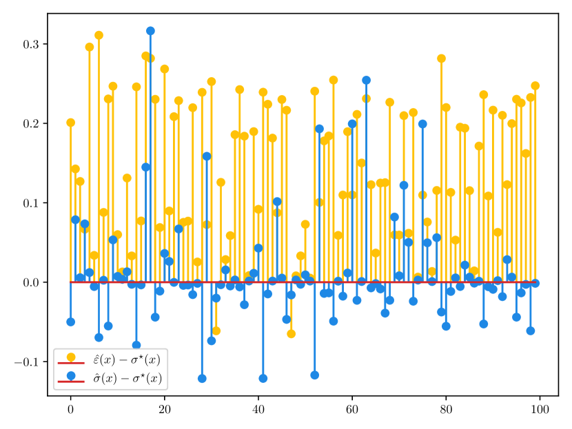
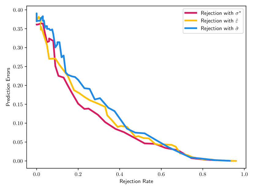
In Figure 3, we illustrate the discrepancy between a standard deviation estimate and our safe approach. Numerical observations indicate that the estimated conditional variance frequently tends to be smaller than its target; while the length of the conformal set is often an upper bound for the standard deviation . This means that if the optimal predictor is uncertain enough to make a prediction, we will also safely abstain; this holds for each data point. In contrast to previous methods, our theoretical analysis holds in finite sample size, with mild assumption on the noise, and for any predictor . Despite being a safer approach for each instance, Figure 3(b) illustrates that, in average, the prediction with conformal abstention is not too conservative.
6 Numerical Experiments
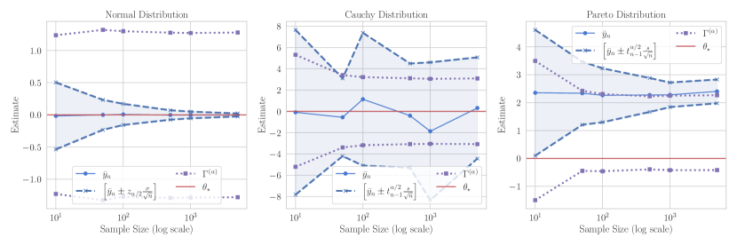
We evaluate our method in the usual setting of linearly distributed data, and compare it to SPS and RII. We emphasize that similarly to previous works (Guille-Escuret and Ndiaye, 2024; Csaji et al., 2015) we only evaluate on synthetic data, because ground truth parameters are not known for real world datasets. Therefor, the validity of coverage bounds can not be confirmed, and the provided guarantees are never valid for distributions that may not be perfectly linear, making confidence regions impossible to compare fairly. We consider four distinct types of noise summarized in Table 1. In all of our experiments, unless stated otherwise, we set , sample from , and the are sampled independently from .
Coverage
In Table 3, the display coverage of various methods. We find that even with chosen based on 2.3, CCR strongly overbounds , with a coverage much above the guaranteed rate. This comes from the CP intervals having a much larger coverage for than for the noisy output . While we seek tight confidence regions, it is beneficial to observe higher than expected coverage as long as the size of remains small. Interestingly, we find that SPS is not capable of producing optimizable confidence regions when the dimension is larger than the training set size.
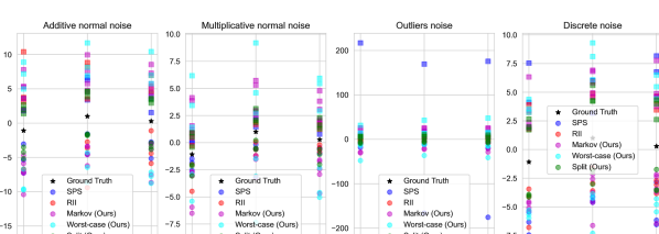
Coordinate intervals
Figure 2 illustrates the lower and upper bounds per coordinate inferred by optimizing over SPS, RII and CCR. The average width for each method and noise, as well as the corresponding computation time, are reported in Table 5. Experiments are run in dimension for the sake of clarity, with a training set of points. For each method, we run independent trials (with fixed ) to visualize the variance of the produced coordinate bounds. We find that while SPS is very fast and performs well on Gaussian noises, its confidence regions tend to be unreliable on less standard noises. While RII is versatile, its computation time for the bounds is high due to the adoption of a low , resulting in more combinatorial complexity for the MILP. Furthermore, we find that Markov and worst-case bounds tend to perform worse than prior works, suggesting that the uncertainty on the distribution of the coverage for black-box CP methods is limiting. The split CP bound achieves a reasonable running time (though much slower than SPS), and produces confidence intervals across noises that are smaller or comparable to other methods, which supports its applicability.
Hypothesis testing
Following (Guille-Escuret and Ndiaye, 2024), we consider the model Using the least square predictor on , we measure whether is empty, rightfully rejecting the linearity hypothesis, and average this rate over trials. CCR outperforms all methods in rejecting linearity. Unlike SPS, it’s noteworthy that CCR can reject linearity, as the least square estimator on is in the confidence region.
Conclusion
We presented CCR, a method for constructing confidence regions under minimal assumptions on the noise, for which we provided finite-sample valid coverage guarantees in different settings. Additional discussions, such as on apparent limitations of our work, can be found in Appendix B
References
- Alcantara and Cysneiros [2017] Izabel Cristina Alcantara and Francisco José A Cysneiros. Slash-elliptical nonlinear regression model. Brazilian Journal of Probability and Statistics, pages 87–110, 2017.
- Angelopoulos et al. [2023] Anastasios N Angelopoulos, Stephen Bates, Clara Fannjiang, Michael I. Jordan, and Tijana Zrnic. Prediction-powered inference. arXiv preprint arXiv:2301.09633, 2023.
- Balzar [1993] Davor Balzar. X-ray diffraction line broadening: modeling and applications to high-tc superconductors. Journal of research of the National Institute of Standards and Technology, 98(3):321, 1993.
- Bernardo and Smith [2009] José M Bernardo and Adrian FM Smith. Bayesian theory, volume 405. John Wiley & Sons, 2009.
- Campi and Weyer [2005] M.C. Campi and E. Weyer. Guaranteed non-asymptotic confidence regions in system identification. Automatica, 41:1751–1764, 2005.
- Castillo [2024] Ismaël Castillo. Bayesian nonparametric statistics, st-flour lecture notes. arXiv preprint arXiv:2402.16422, 2024.
- Chen et al. [2015] Yuan Chen, Ercan Engin Kuruoglu, and Hing Cheung So. Optimum linear regression in additive cauchy–gaussian noise. Signal processing, 106:312–318, 2015.
- Chernozhukov et al. [2021] Victor Chernozhukov, Kaspar Wüthrich, and Yinchu Zhu. Distributional conformal prediction. Proceedings of the National Academy of Sciences, 118(48):e2107794118, 2021.
- Cherubin [2019] Giovanni Cherubin. Majority vote ensembles of conformal predictors. Machine Learning, 108(3):475–488, 2019.
- Chow [1994] CK Chow. Recognition error and reject trade-off. Technical report, Nevada Univ., Las Vegas, NV (United States), 1994.
- Csaji et al. [2015] Balazs Csanad Csaji, Marco Claudio Campi, and Erik Weyer. Sign-perturbed sums: A new system identification approach for constructing exact non-asymptotic confidence regions in linear regression models. IEEE Transactions on Signal Processing, 63, jan 2015.
- Dalai et al. [2007] Marco Dalai, Erik Weyer, and Marco C. Campi. Parameter identification for nonlinear systems: Guaranteed confidence regions through lscr. Automatica, 43, 2007.
- Daniels [1954] H. E. Daniels. A Distribution-Free Test for Regression Parameters. The Annals of Mathematical Statistics, 25, 1954.
- den Dekker et al. [2008] Arnold J. den Dekker, Xavier Bombois, and Paul M.J. Van den Hof. Finite sample confidence regions for parameters in prediction error identification using output error models. IFAC Proceedings Volumes, 41, 2008.
- Farsad et al. [2015] Nariman Farsad, Weisi Guo, Chan-Byoung Chae, and Andrew Eckford. Stable distributions as noise models for molecular communication. In 2015 IEEE Global Communications Conference (GLOBECOM), pages 1–6. IEEE, 2015.
- Feldman et al. [2023] Shai Feldman, Bat-Sheva Einbinder, Stephen Bates, Anastasios N Angelopoulos, Asaf Gendler, and Yaniv Romano. Conformal prediction is robust to dispersive label noise. In Conformal and Probabilistic Prediction with Applications, pages 624–626. PMLR, 2023.
- Fong and Holmes [2021] Edwin Fong and Chris C Holmes. Conformal Bayesian computation. In NeurIPS, 2021.
- Gasparin and Ramdas [2024] Matteo Gasparin and Aaditya Ramdas. Merging uncertainty sets via majority vote, 2024.
- Geifman and El-Yaniv [2019] Yonatan Geifman and Ran El-Yaniv. Selectivenet: A deep neural network with an integrated reject option. In International conference on machine learning, pages 2151–2159. PMLR, 2019.
- Gibbs and Candès [2022] Isaac Gibbs and Emmanuel Candès. Conformal inference for online prediction with arbitrary distribution shifts. arXiv preprint arXiv:2208.08401, 2022.
- Guha et al. [2024] Etash Guha, Shlok Natarajan, Thomas Möllenhoff, Mohammad Emtiyaz Khan, and Eugene Ndiaye. Conformal prediction via regression-as-classification. arXiv preprint arXiv:2404.08168, 2024.
- Guille-Escuret and Ndiaye [2024] Charles Guille-Escuret and Eugene Ndiaye. Finite sample confidence regions for linear regression parameters using arbitrary predictors. arXiv preprint arXiv:2401.15254, 2024.
- Hillier and Lieberman [2001] F.S. Hillier and G.J. Lieberman. Introduction to Operations Research. McGraw-Hill, 2001.
- Hulsman [2022] Roel Hulsman. Distribution-free finite-sample guarantees and split conformal prediction, 2022.
- Jochmans [2022] Koen Jochmans. Heteroscedasticity-robust inference in linear regression models with many covariates. Journal of the American Statistical Association, 117, 2022.
- Lei et al. [2013] Jing Lei, James Robins, and Larry Wasserman. Distribution-free prediction sets. Journal of the American Statistical Association, 108(501):278–287, 2013.
- Lei et al. [2018] Jing Lei, Max G’Sell, Alessandro Rinaldo, Ryan J Tibshirani, and Larry Wasserman. Distribution-free predictive inference for regression. Journal of the American Statistical Association, 113(523):1094–1111, 2018.
- Lin et al. [2022] Zhen Lin, Shubhendu Trivedi, and Jimeng Sun. Conformal prediction intervals with temporal dependence. arXiv preprint arXiv:2205.12940, 2022.
- Linusson et al. [2018] Henrik Linusson, Ulf Johansson, Henrik Boström, and Tuve Löfström. Classification with reject option using conformal prediction. In Advances in Knowledge Discovery and Data Mining: 22nd Pacific-Asia Conference, PAKDD 2018, Melbourne, VIC, Australia, June 3-6, 2018, Proceedings, Part I 22, pages 94–105. Springer, 2018.
- Pagnini and Mainardi [2010] Gianni Pagnini and Francesco Mainardi. Evolution equations for the probabilistic generalization of the voigt profile function. Journal of computational and applied mathematics, 233(6):1590–1595, 2010.
- Papadopoulos et al. [2002] Harris Papadopoulos, Kostas Proedrou, Volodya Vovk, and Alex Gammerman. Inductive confidence machines for regression. In Machine Learning: ECML 2002: 13th European Conference on Machine Learning Helsinki, Finland, August 19–23, 2002 Proceedings 13. Springer, 2002.
- Ramdas and Manole [2023] Aaditya Ramdas and Tudor Manole. Randomized and exchangeable improvements of markov’s, chebyshev’s and chernoff’s inequalities, 2023.
- Rogers and Tukey [1972] William H Rogers and John W Tukey. Understanding some long-tailed symmetrical distributions. Statistica Neerlandica, 26(3):211–226, 1972.
- Romano et al. [2019a] Y. Romano, E. Patterson, and E. J. Candes. Conformalized quantile regression. In NeurIPS, 2019a.
- Romano et al. [2019b] Yaniv Romano, Evan Patterson, and Emmanuel Candes. Conformalized quantile regression. In Advances in Neural Information Processing Systems, 2019b.
- Shafer and Vovk [2008] G. Shafer and V. Vovk. A tutorial on conformal prediction. Journal of Machine Learning Research, 2008.
- Taquet et al. [2022] Vianney Taquet, Vincent Blot, Thomas Morzadec, Louis Lacombe, and Nicolas Brunel. Mapie: an open-source library for distribution-free uncertainty quantification. arXiv preprint arXiv:2207.12274, 2022.
- Tsybakov [2009] Alexandre B Tsybakov. Nonparametric estimators. Introduction to Nonparametric Estimation, pages 1–76, 2009.
- Van der Vaart [2000] Aad W Van der Vaart. Asymptotic statistics, volume 3. Cambridge university press, 2000.
- Vovk [2012] Vladimir Vovk. Conditional validity of inductive conformal predictors. In Asian conference on machine learning, pages 475–490. PMLR, 2012.
- Wald [1939] Abraham Wald. Contributions to the theory of statistical estimation and testing hypotheses. The Annals of Mathematical Statistics, 10, 1939.
- Wald [1945] Abraham Wald. Statistical decision functions which minimize the maximum risk. Annals of Mathematics, 46, 1945.
- Wasserman [2006] Larry Wasserman. All of nonparametric statistics. Springer Science & Business Media, 2006.
- Wasserman et al. [2020a] Larry Wasserman, Aaditya Ramdas, and Sivaraman Balakrishnan. Universal inference. Proceedings of the National Academy of Sciences, 117:16880–16890, 2020a.
- Wasserman et al. [2020b] Larry Wasserman, Aaditya Ramdas, and Sivaraman Balakrishnan. Universal inference. Proceedings of the National Academy of Sciences, 117(29):16880–16890, 2020b.
- Wolsey and Nemhauser [2014] L.A. Wolsey and G.L. Nemhauser. Integer and Combinatorial Optimization. Wiley, 2014.
- Zaffran et al. [2022] Margaux Zaffran, Olivier Féron, Yannig Goude, Julie Josse, and Aymeric Dieuleveut. Adaptive conformal predictions for time series. In International Conference on Machine Learning, pages 25834–25866. PMLR, 2022.
- Zaoui et al. [2020] Ahmed Zaoui, Christophe Denis, and Mohamed Hebiri. Regression with reject option and application to knn. Advances in Neural Information Processing Systems, 33, 2020.
Appendix A Additional Experiments
Table 6 gives an extended version of Table 2 over a wider variety of settings, with the same conclusions.
| CP Method | Train Size | Noise | # Losses | ||
|---|---|---|---|---|---|
| Residual | 40 | Gaussian | |||
| Outliers | |||||
| Mult. Gaussian | |||||
| 100 | Gaussian | ||||
| Outliers | |||||
| Mult. Gaussian | |||||
| Quantile | 40 | Gaussian | |||
| Outliers | |||||
| Mult. Gaussian | |||||
| 100 | Gaussian | ||||
| Outliers | |||||
| Mult. Gaussian |
Appendix B Additional Discussions
We introduced CCR, a method for aggregating conformal prediction intervals into finite-sample valid confidence regions on model parameters, adaptable to diverse noise types. For linear models, the resulting confidence region can be formulated as an MILP, showing competitiveness with previous approaches in various downstream applications. In the following, we discuss some of the critical drawbacks of the proposed methods.
B.1 Limitations
B.1.1 Model well-specification
Our approach begins with the explicit relation between inputs and outputs, as stated in Equation 1. If this relation is incorrect, namely in the case of model misspecification, our claims will not hold. Nevertheless, in contrast to previous approaches, the departure from this core assumption is controlled by the parameter , which is assumed to be known. Incorrectly setting this parameter can lead to unreliable results. This is to be contrasted with the assumption that the shape of the noise distribution is known, which is a significantly stronger assumption than the one made here.
B.1.2 Inadequacy in high dimensional regime
Our main goal is to provide systematic way of building confidence sets for model parameters for data-driven prediction methods. Our theory comes with explicit bounds that tightly quantify the coverage we can guarantee. However, good coverage does not necessarily align with efficiency (ie small enough confident region) and a trade-off between the two might be necessary. As we displayed the coverage curves in Figure 1 and illustrated the boundness of our uncertainty region for linear models, we must restrict the application to small enough dimension in order to maintain a reasonable efficiency. As a consequence, our method is of limited used in modern deep learning models.
B.1.3 Suboptimality wrt standard methods in the well behaved distribution settings
Consider a sequence of iid variable following a gaussian distribution where for simplicity we suppose that the standard deviation is known. In that case, the ground-truth can be estimated with the empirical mean and we know exactly the distribution of the estimation error . Thus, a confidence interval for the model parameter is obtained as
| (11) |
Similar strategy can be used to sequentially build prediction sets for the outputs. Indeed, we have and . As such, we can also characterize the distribution of errors . Thus, a prediction set is obtained as
| (12) |
Following our strategy, we should exploit the knowledge and then
and finally
| (13) |
As one can see, the interval Equation 11 is much better than Equation 13 as the former shrink to a point mass while the latter does not. Also, both are affected by the standard deviation .
However, that’s not exactly what we are doing. We can avoid being affected by . Indeed our approach still hold even when . First, notice that using Equation 12 directly with Equation 4 reads
| (14) |
This mean that explicitly exploiting the shape of the distribution instead of its sole symmetry might not be a good idea because, the set does not shrink to a point mass while still being affected, explicitly, by the standard deviation. This does not allows to handle cases where the variance is infinite.
Leveraging Conformal Prediction set
Now we make no further assumption beside which is true for gaussian distribution. Our base predictor is the empirical mean and the score function is simply the distance to the mean (any estimator can be used e.g. median can be used) ie
It is easy to see that . Defining as the -quantile of , the -conformal set for is given by:
Our result Equation 4 (resp. The split CP version) reads
Even if for a given dataset, the radius is always finite, it will be large if the variance of the underlying distribution is large. This occurs because the base predictor may have difficulty accurately predicting the targets, resulting in large score functions.
Appendix C Proofs
In this section, we provide detailed proofs for the propositions outlined in the main paper.
C.1 Coverage of the noiseless output
*
Proof.
For simplicity, let us denote and . We have
Injecting above, and upper bounding with , we obtain
Or equivalently,
Which concludes the proof. ∎
C.2 Lower bounds on the expected coverage
*
Proof.
It holds
and
| (15) |
Since the are assumed to be sampled independently, it is easy to see that conditionally on , is independent from for . Thus, Equation 15 can be rewritten as
Now it only remains to use Jensen’s inequality to find that
Concluding the proof. ∎
*
Proof.
Let
The structure of the proof is as follow. We first prove that given a feasible , it is possible to shrink the support set of around two values and while preserving and preserving or decreasing .
Let such that .
We want to prove that there exists and such that and . If is constant, then we can take with . Else, let
and
Since is not constant, there are some for which it is larger than its expectation, and some for which it is smaller, thus and . Let us denote
with and . Let us consider . We now split into and . We now want to find such that
| (16) |
can for instance be constructed by taking and considering the set where represents the ball of center and radius for the euclidean metric, viewing as an element of , and increasing until reaching . In that construction, decreases monotonously and continuously (since is a continuous R.V.), and for it is the expectation over which is larger than by construction, while for sufficiently large we get which is smaller than because we are only removing elements of which are all larger than . Hence, by intermediate value theorem, there is indeed an such that Equation 16 is satisfied.
We now consider and .
Let
Let us assume for instance that .
We now want to define a projection from to preserving relative probabilities. For convenience, let be an order on , such as the dictionary order, the cumulative distribution function on for that order, and the quantile function on . We define . We then have
And thus
Let us finally consider defined by and .
We have
Similarly
Finally, only take values in , thus, , as the diameter of is half that of by construction. If , we can follow the same process except that we project into . If , we can follow the same process except that we divide around its center instead of .
By repeating the process we find a sequence of for which is at most , the expectation over is , and both and shrink to singletons and .
Then, by introducing ,
where is the quantile function of for the dictionary order, we get that is feasible (it has expectation exactly ) and , with .
By introducing and
satisfies the constraint and for any feasible , .
This concludes the proof.
∎
C.2.1 Analytical expression for the lower bound with split CP
Lemma C.2 provides a closed form expression to compute the bound in the case of split CP.
Let us start with two intermediate lemmas that provide the expected value of the exceed when the probability follows a Beta distribution.
Lemma C.1.
Proof.
Hence the result, since . ∎
Lemma C.2.
Proof.
We denote . As such if and only if and we have
where in the second equality, we use and denoted
∎
propositionweaksplit Let be the Beta function and the incomplete version
Proof.
C.3 High Probability Lower Bounds
Valid coverage does not always holds conditional on the observed data, so we might settle for a high probability guarantee rather than an expected one. Notably, the lower bound in 2.2 also holds conditionally on . Thus, , a Probably Approximately Correct guarantees on the coverage of the noisy outputs [Vovk, 2012] translate into the noiseless output as well.
We illustrate in Figure 6, how the coverage changes as a function of .
Lemma C.3.
Under the model in Equation 1, It holds
propositionpaccoverage For any , let us define . Then, it holds
Furthermore, we also have
where
Proof.
Since the events are independent and occurs with probability , we have
And since with probability , we have with probability at least over
by construction of , which concludes the proof. ∎
Remark C.4.
From Equation 10, one also obtains the more accurate PAC lower bound with
where is the c.d.f. of distribution.
C.3.1 Conformal abstention
*
Proof.
By definition, we have if and only if and . Thus,
∎
C.4 MILP representation
*
Proof.
By definition,
To capture that such constraint should only be active when , we use the big M method [Wolsey and Nemhauser, 2014, Hillier and Lieberman, 2001], that sets a large constant and applying the constraint ()
One verifies that all the constraints for which are inactive, and increase otherwise, to ensure the equivalence of the feasible set. ∎
Appendix D Other
D.1 Counter-example to 2.3
While 2.3 is very likely to hold, it cannot be theoretically guaranteed, due to adversarial counter-examples.
For instance, consider the following simple 1D counter-example:
and
In this case, when , covers both the noisy and noise-free output with probability 1. When , never contains the noise-free output , but contains the noisy output with probability 0.5 (when ). As such, the coverage of for the noisy output is 0.95, while its coverage for the noise free output is 0.9.